Embed Size (px)
Citation preview
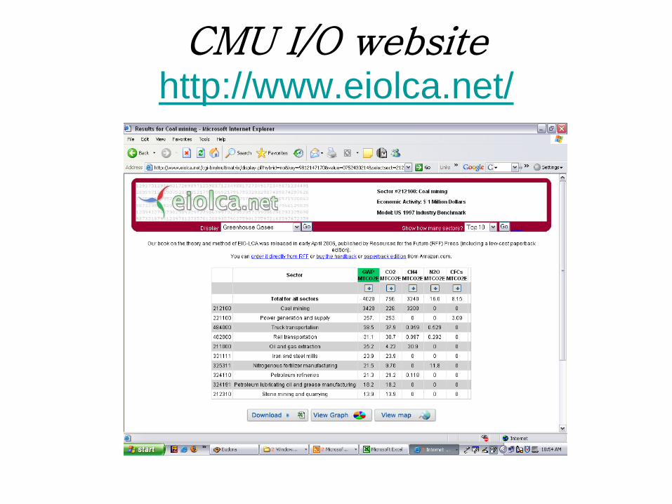
LCA/LCI Examples 2.83/2.813
Mining
Manufacturing
Use Phase End of Life
T. Gutowski
Outline
1. Comparisons between possible substitutes
– Plug-in Hybrid Cars
– Alternative PV Technologies
2. Substitutes and Compliments
– Conference calls and travel
3. Moving beyond comparisons -consequences
4. Environmental Lifestyle Analysis (ELSA)
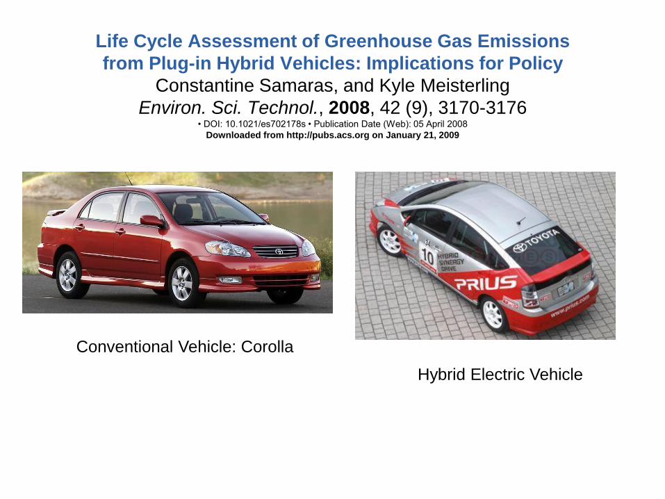
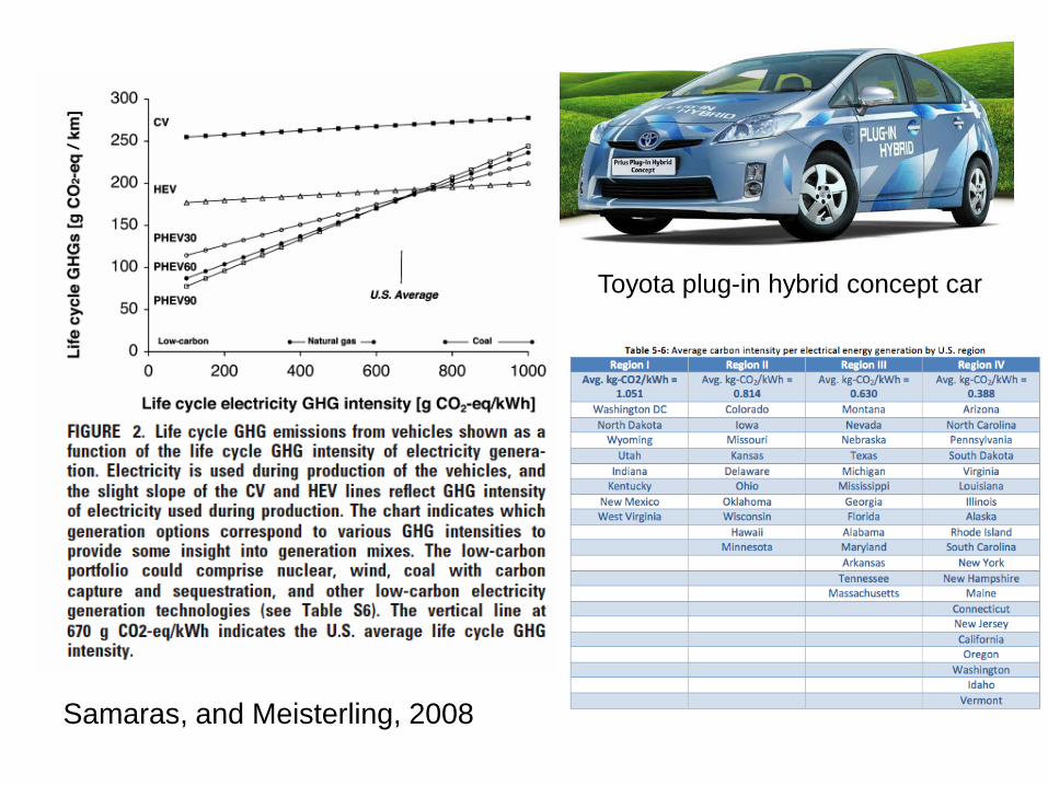
Life Cycle Assessment of Greenhouse Gas Emissions
from Plug-in Hybrid Vehicles: Implications for Policy
Constantine Samaras, and Kyle Meisterling
Environ. Sci. Technol., 2008, 42 (9), 3170-3176 • DOI: 10.1021/es702178s • Publication Date (Web): 05 April 2008
Downloaded from http://pubs.acs.org on January 21, 2009
Conventional Vehicle: Corolla
Hybrid Electric Vehicle
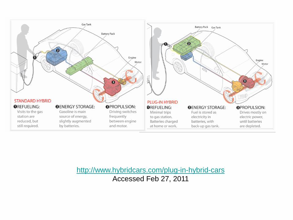
http://www.hybridcars.com/plug-in-hybrid-cars
Accessed Feb 27, 2011
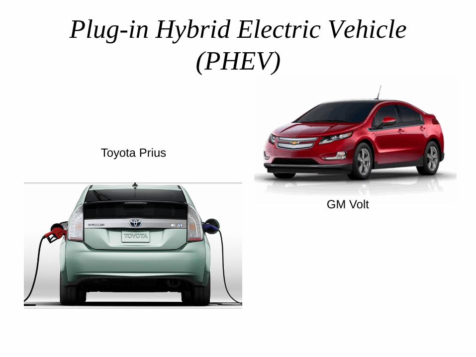
Plug-in Hybrid Electric Vehicle
(PHEV)
GM Volt
Toyota Prius

Hybrid Study
• Three alternatives:
– ICE, HEV, PHEV
• EIOLCA + Li ion battery
• Three grid scenarios
– 200, 670, and 950 gCO2/kWh
• 150,000 miles (240,000 km)
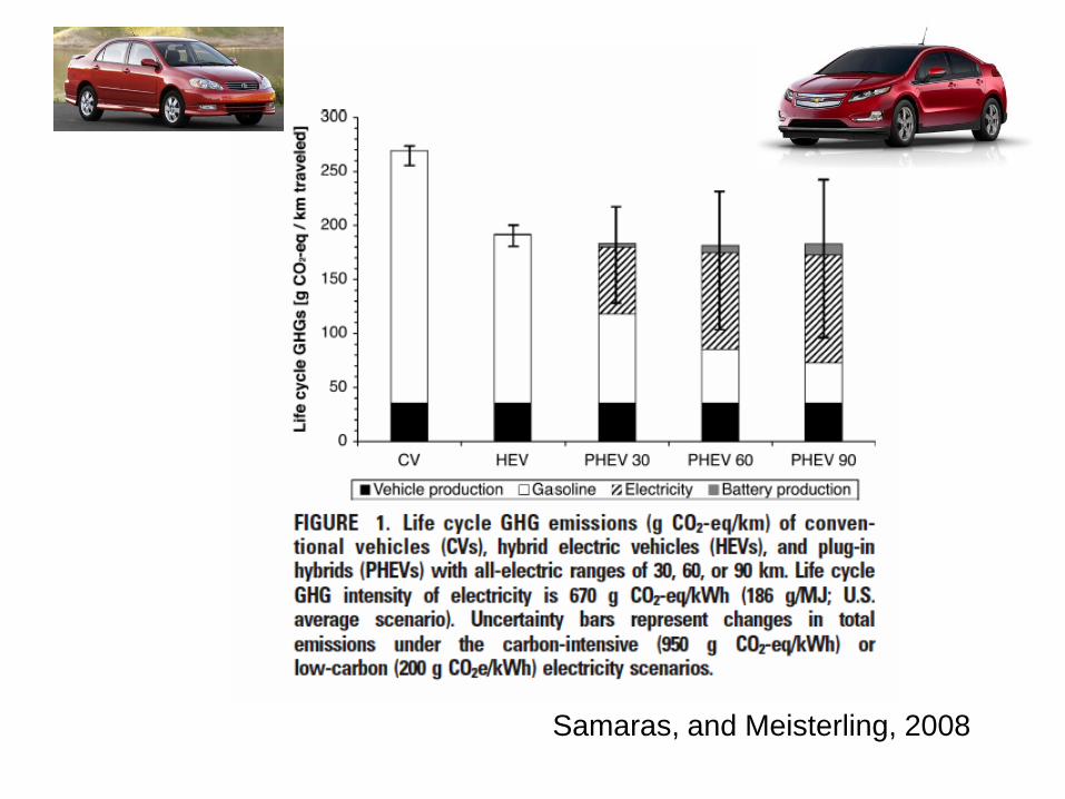
Samaras, and Meisterling, 2008
Samaras, and Meisterling, 2008
Toyota plug-in hybrid concept car
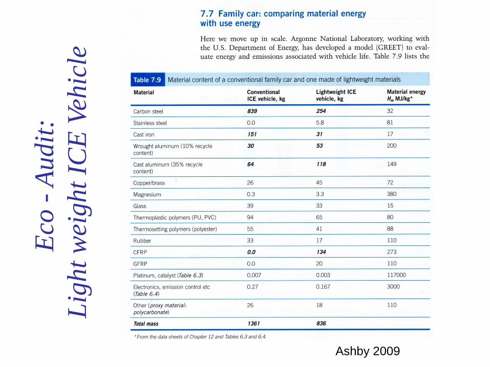
“Eco-Audit” E
co -
Au
dit
:
Lig
ht
wei
gh
t IC
E V
ehic
le
Ashby 2009
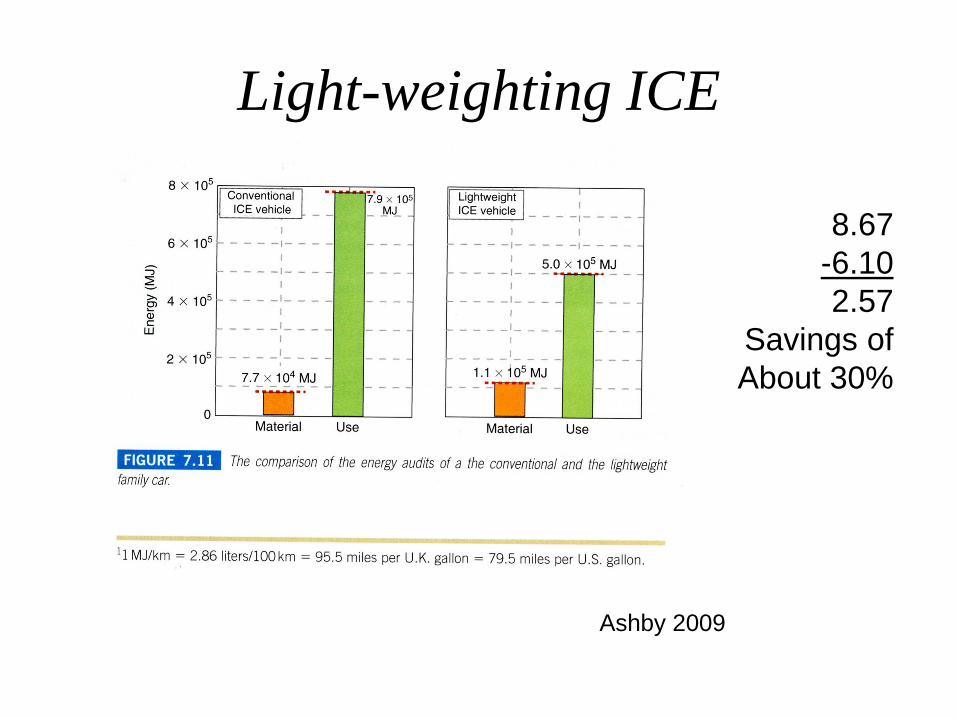
Light-weighting ICE
Ashby 2009
8.67
-6.10
2.57
Savings of
About 30%
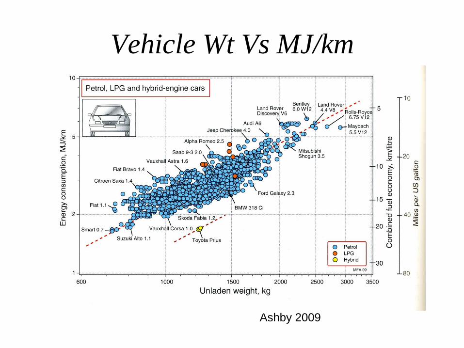
Vehicle Wt Vs MJ/km
Ashby 2009
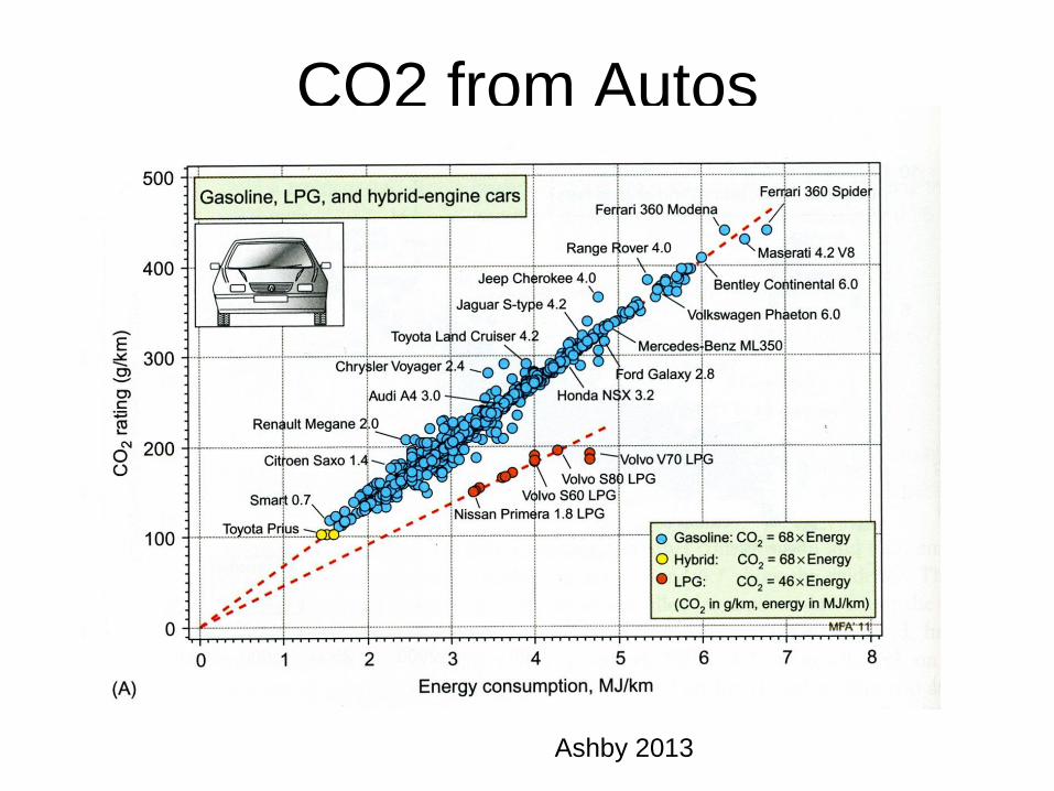
CO2 from Autos
Ashby 2013
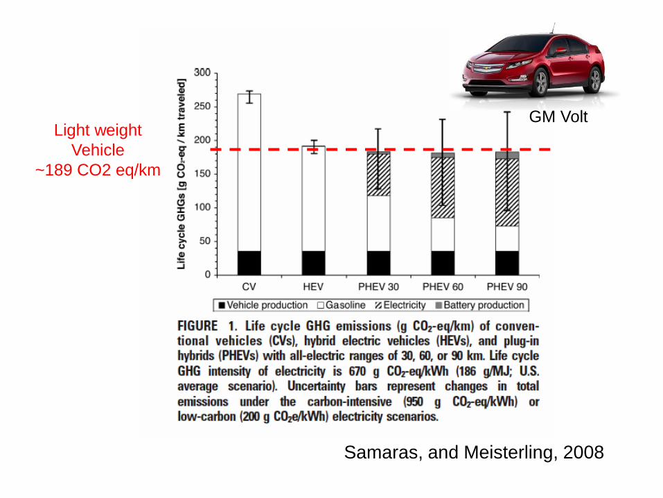
Samaras, and Meisterling, 2008
GM Volt Light weight
Vehicle
~189 CO2 eq/km
Main Points
• It depends!
• PHEVs reduce dependence on liquid fuels
and may give biofuels a chance
• But how this plays out depends strongly
on how the grid develops
• Issues
– Batteries and range
– Air pollutants and toxic releases
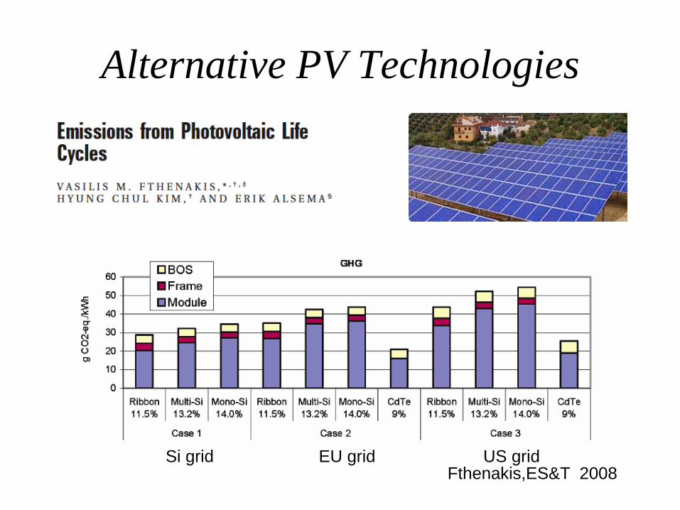
Alternative PV Technologies
Fthenakis,ES&T 2008 US grid EU grid Si grid
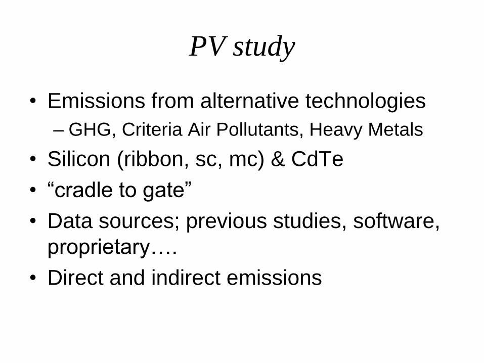
PV study
• Emissions from alternative technologies
– GHG, Criteria Air Pollutants, Heavy Metals
• Silicon (ribbon, sc, mc) & CdTe
• “cradle to gate”
• Data sources; previous studies, software,
proprietary….
• Direct and indirect emissions
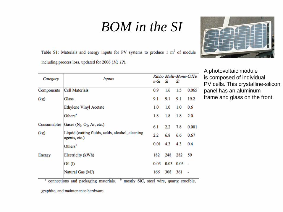
BOM in the SI
A photovoltaic module
is composed of individual
PV cells. This crystalline-silicon
panel has an aluminum
frame and glass on the front.
Fthenakis,ES&T 2008
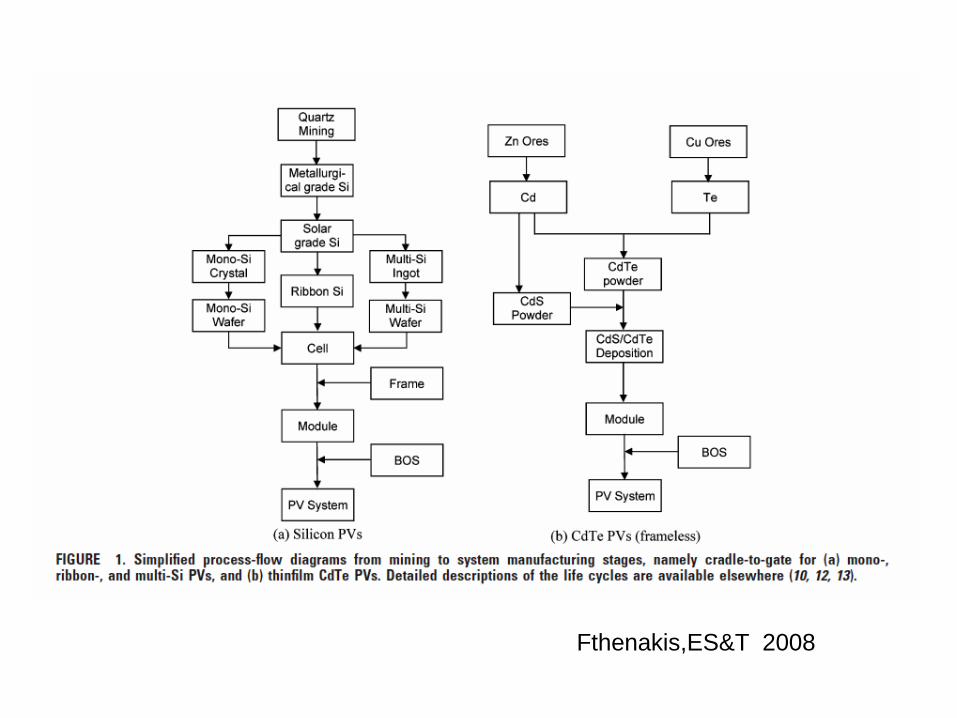
Fthenakis, ES&T 2008
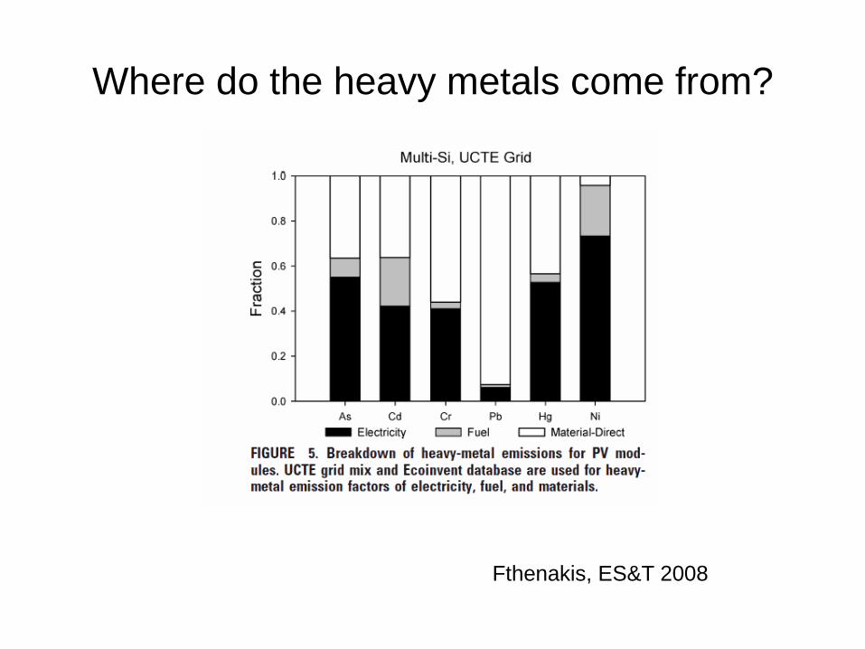
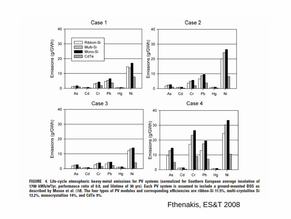
Where do the heavy metals come from?
Fthenakis, ES&T 2008
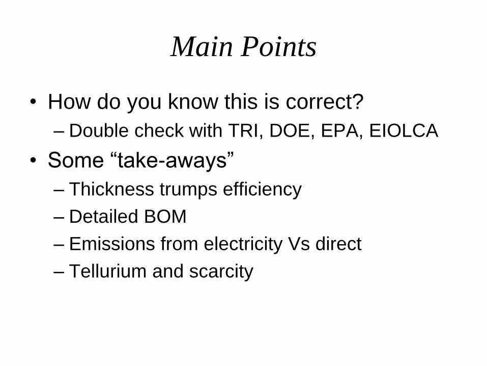
Main Points
• How do you know this is correct?
– Double check with TRI, DOE, EPA, EIOLCA
• Some “take-aways”
– Thickness trumps efficiency
– Detailed BOM
– Emissions from electricity Vs direct
– Tellurium and scarcity
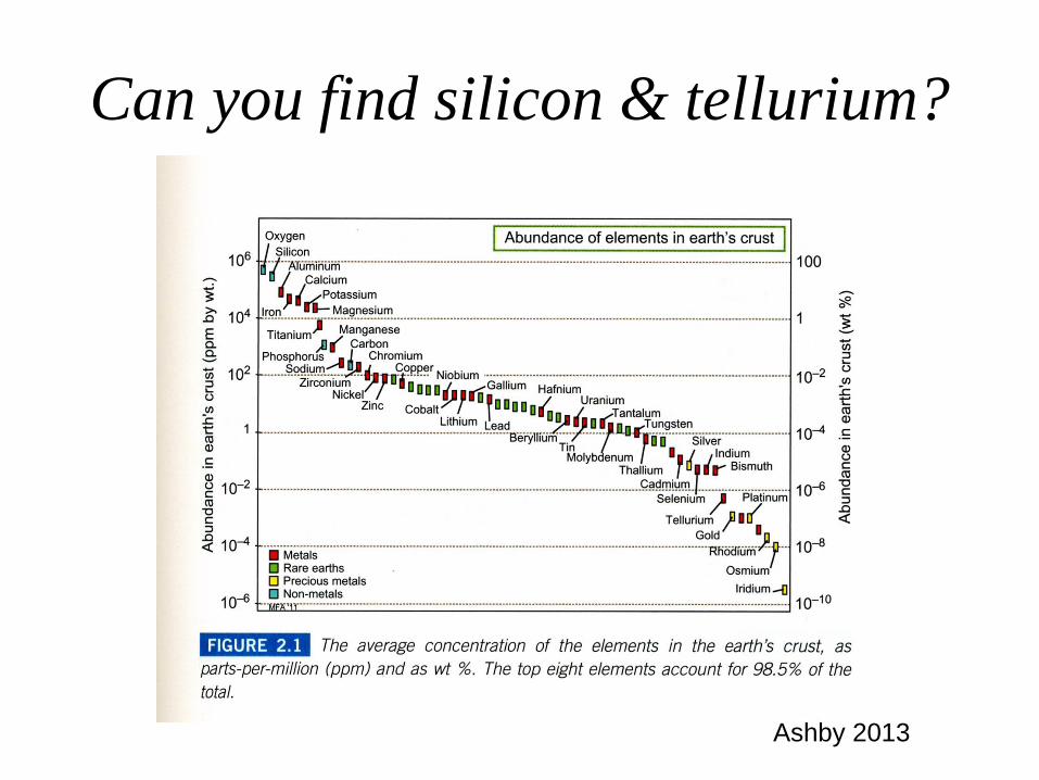
Can you find silicon & tellurium?
Ashby 2013
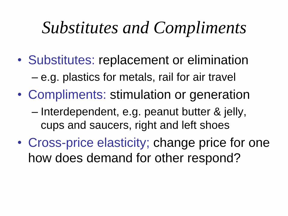
Substitutes and Compliments
• Substitutes: replacement or elimination
– e.g. plastics for metals, rail for air travel
• Compliments: stimulation or generation
– Interdependent, e.g. peanut butter & jelly,
cups and saucers, right and left shoes
• Cross-price elasticity; change price for one
how does demand for other respond?
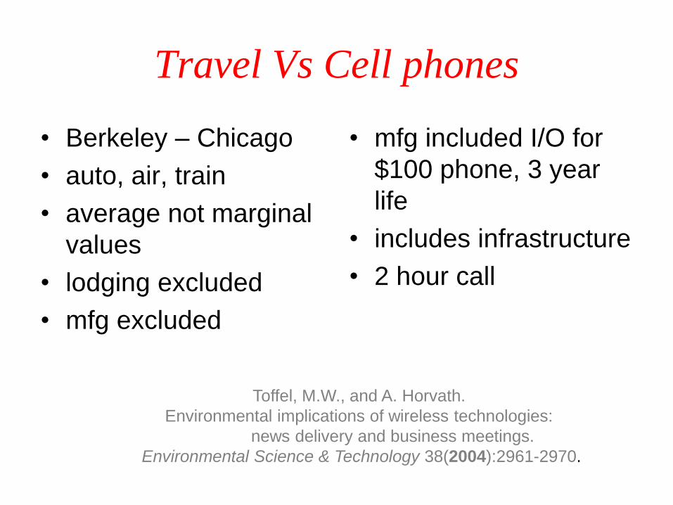
Travel Vs Cell phones
• Berkeley – Chicago
• auto, air, train
• average not marginal
values
• lodging excluded
• mfg excluded
• mfg included I/O for
$100 phone, 3 year
life
• includes infrastructure
• 2 hour call
Toffel, M.W., and A. Horvath.
Environmental implications of wireless technologies:
news delivery and business meetings.
Environmental Science & Technology 38(2004):2961-2970.

Travel Vs Cell phones
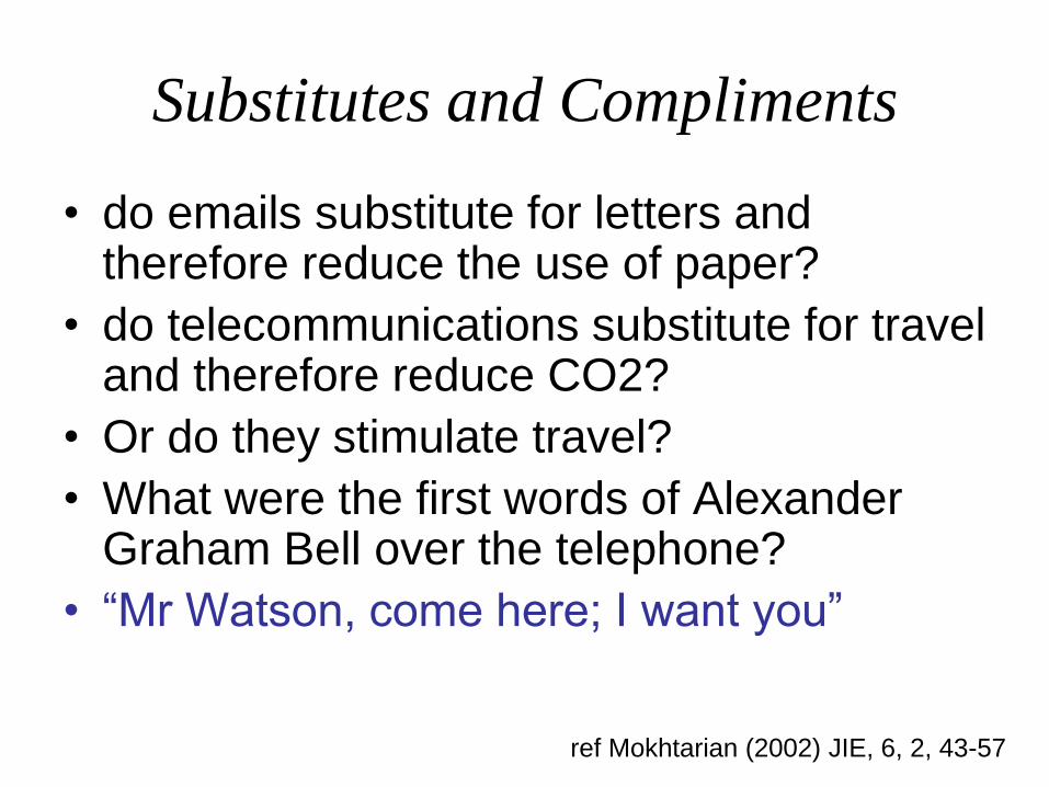
Substitutes and Compliments
• do emails substitute for letters and therefore reduce the use of paper?
• do telecommunications substitute for travel and therefore reduce CO2?
• Or do they stimulate travel?
• What were the first words of Alexander Graham Bell over the telephone?
• “Mr Watson, come here; I want you”
ref Mokhtarian (2002) JIE, 6, 2, 43-57

Outline
1. Comparisons between possible substitutes
– Plug-in Hybrid Cars
– Alternative PV Technologies
2. Substitutes and Compliments
– Conference calls and travel
3. Moving beyond comparisons to consequences
4. Environmental Lifestyle Analysis (ELSA)
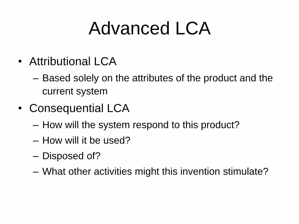
Advanced LCA
• Attributional LCA
– Based solely on the attributes of the product and the
current system
• Consequential LCA
– How will the system respond to this product?
– How will it be used?
– Disposed of?
– What other activities might this invention stimulate?
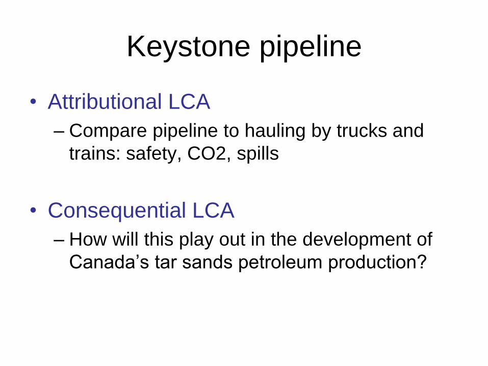
Keystone pipeline
• Attributional LCA
– Compare pipeline to hauling by trucks and
trains: safety, CO2, spills
• Consequential LCA
– How will this play out in the development of
Canada’s tar sands petroleum production?
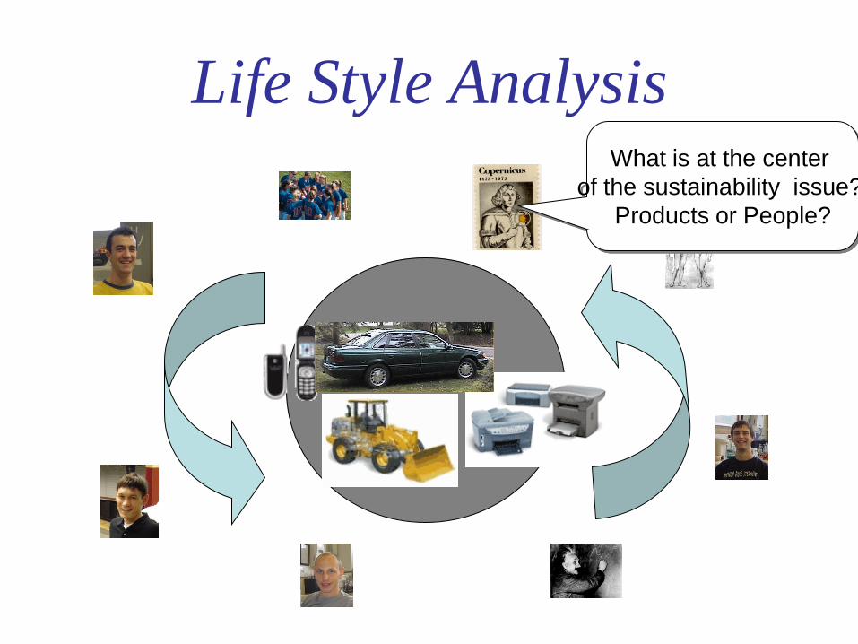
Life Style Analysis What is at the center
of the sustainability issue?
Products or People?

Environmental Life Style Analysis
(ELSA)
Timothy Gutowski, Amanda Taplett, Anna Allen, Amy Banzaert, Rob Cirinciore,
Christopher Cleaver, Stacy Figueredo, Susan Fredholm, Betar Gallant, Alissa Jones,
Jonathan Krones, Barry Kudrowitz, Cynthia Lin, Alfredo Morales, David Quinn,
Megan Roberts, Robert Scaringe, Tim Studley, Sittha Sukkasi, Mika Tomczak,
Jessica Vechakul, and Malima Wolf, Anthony Texixeira and Mitchell Westwood.
Proceedings:
IEEE International Symposium on Electronics
and the Environment, San Francisco, USA May 19 – 21, 2008
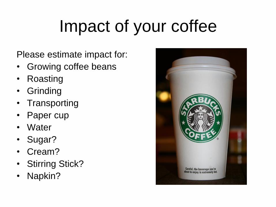
Impact of your coffee
Please estimate impact for:
• Growing coffee beans
• Roasting
• Grinding
• Transporting
• Paper cup
• Water
• Sugar?
• Cream?
• Stirring Stick?
• Napkin?
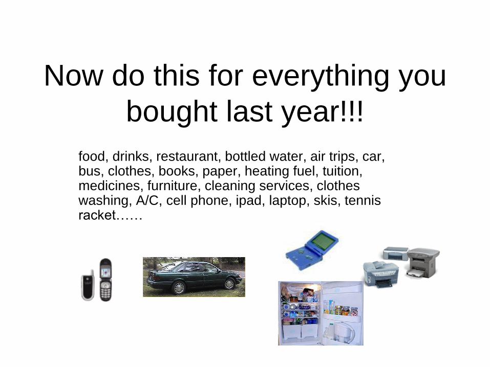
Now do this for everything you
bought last year!!!
food, drinks, restaurant, bottled water, air trips, car, bus, clothes, books, paper, heating fuel, tuition, medicines, furniture, cleaning services, clothes washing, A/C, cell phone, ipad, laptop, skis, tennis racket……
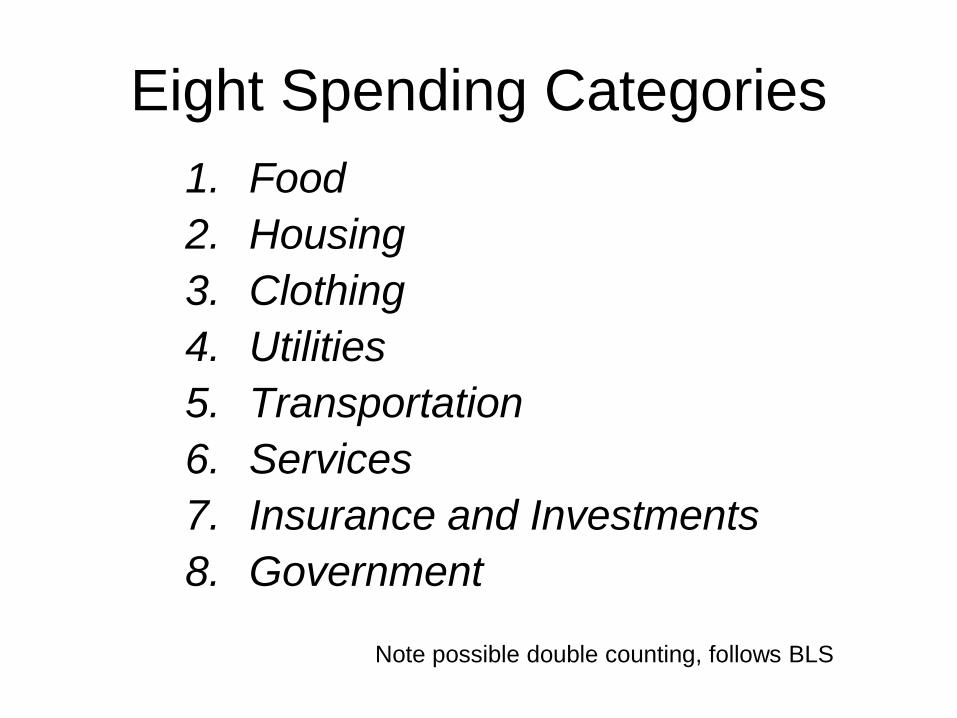
Eight Spending Categories
1. Food
2. Housing
3. Clothing
4. Utilities
5. Transportation
6. Services
7. Insurance and Investments
8. Government
Note possible double counting, follows BLS
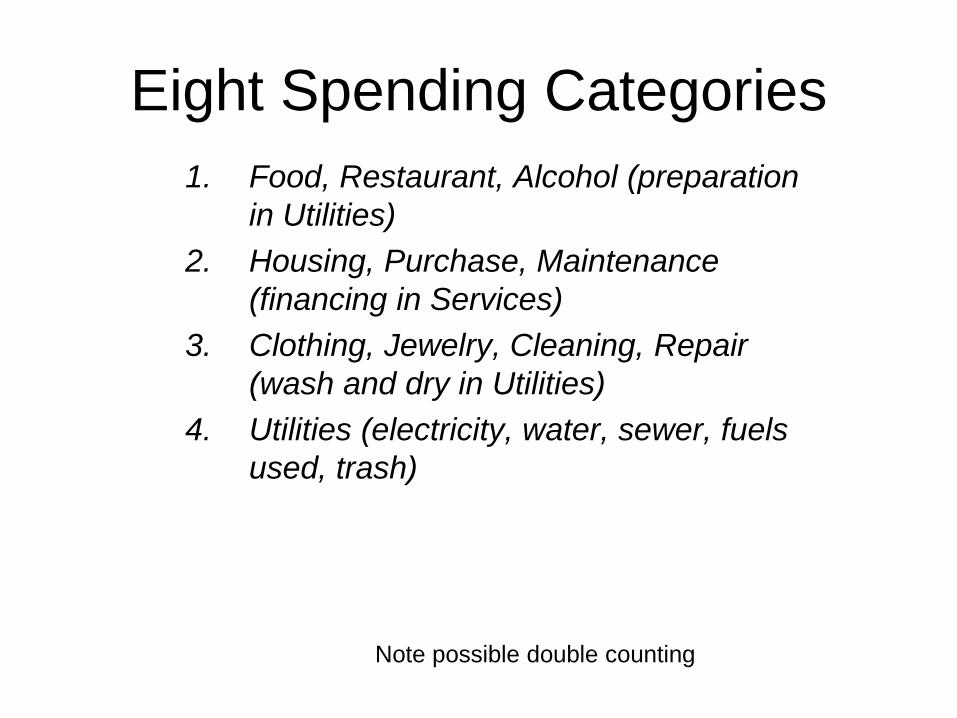
Eight Spending Categories
1. Food, Restaurant, Alcohol (preparation
in Utilities)
2. Housing, Purchase, Maintenance
(financing in Services)
3. Clothing, Jewelry, Cleaning, Repair
(wash and dry in Utilities)
4. Utilities (electricity, water, sewer, fuels
used, trash)
Note possible double counting
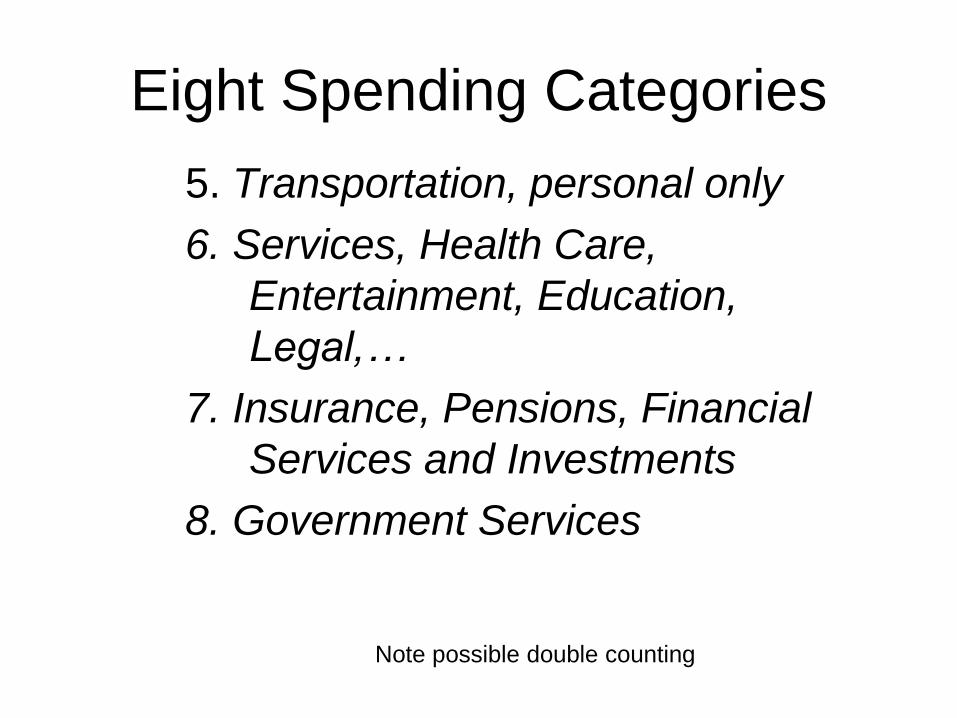
Eight Spending Categories
5. Transportation, personal only
6. Services, Health Care,
Entertainment, Education,
Legal,…
7. Insurance, Pensions, Financial
Services and Investments
8. Government Services
Note possible double counting
Data for all people in the US
is available at the Bureau of
Labor Statistics
http://www.bls.gov/
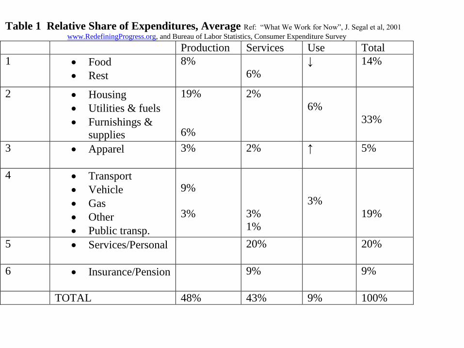
Table 1 Relative Share of Expenditures, Average Ref: “What We Work for Now”, J. Segal et al, 2001
www.RedefiningProgress.org, and Bureau of Labor Statistics, Consumer Expenditure Survey Production Services Use Total
1 Food
Rest
8%
6%
↓ 14%
2 Housing
Utilities & fuels
Furnishings &
supplies
19%
6%
2%
6%
33%
3 Apparel
3% 2% ↑ 5%
4 Transport
Vehicle
Gas
Other
Public transp.
9%
3%
3%
1%
3%
19%
5 Services/Personal
20% 20%
6 Insurance/Pension
9% 9%
TOTAL 48% 43% 9% 100%
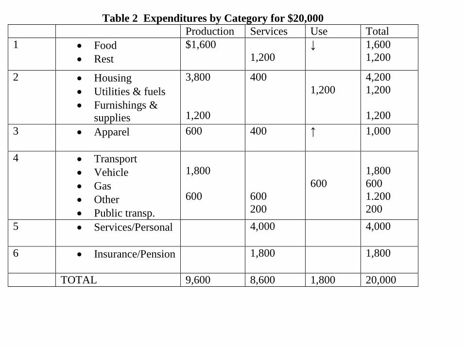
Table 2 Expenditures by Category for $20,000
Production Services Use Total
1 Food
Rest
$1,600
1,200
↓ 1,600
1,200
2 Housing
Utilities & fuels
Furnishings &
supplies
3,800
1,200
400
1,200
4,200
1,200
1,200
3 Apparel
600 400 ↑ 1,000
4 Transport
Vehicle
Gas
Other
Public transp.
1,800
600
600
200
600
1,800
600
1.200
200
5 Services/Personal
4,000 4,000
6 Insurance/Pension
1,800 1,800
TOTAL 9,600 8,600 1,800 20,000
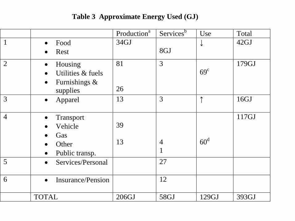
Table 3 Approximate Energy Used (GJ)
Productiona Services
b Use Total
1 Food
Rest
34GJ
8GJ
↓ 42GJ
2 Housing
Utilities & fuels
Furnishings &
supplies
81
26
3
69c
179GJ
3 Apparel
13 3 ↑ 16GJ
4 Transport
Vehicle
Gas
Other
Public transp.
39
13
4
1
60d
117GJ
5 Services/Personal
27
6 Insurance/Pension
12
TOTAL 206GJ 58GJ 129GJ 393GJ
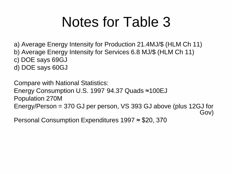
Notes for Table 3
a) Average Energy Intensity for Production 21.4MJ/$ (HLM Ch 11)
b) Average Energy Intensity for Services 6.8 MJ/$ (HLM Ch 11)
c) DOE says 69GJ
d) DOE says 60GJ
Compare with National Statistics:
Energy Consumption U.S. 1997 94.37 Quads ≈100EJ
Population 270M
Energy/Person = 370 GJ per person, VS 393 GJ above (plus 12GJ for Gov)
Personal Consumption Expenditures 1997 ≈ $20, 370
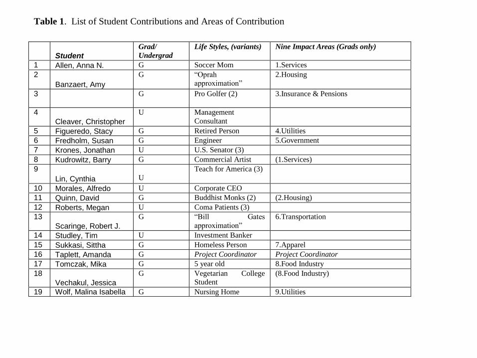
Table 1. List of Student Contributions and Areas of Contribution
Student
Grad/
Undergrad
Life Styles, (variants) Nine Impact Areas (Grads only)
1 Allen, Anna N. G Soccer Mom 1.Services
2
Banzaert, Amy
G “Oprah approximation”
2.Housing
3 G Pro Golfer (2) 3.Insurance & Pensions
4
Cleaver, Christopher
U Management
Consultant
5 Figueredo, Stacy G Retired Person 4.Utilities
6 Fredholm, Susan G Engineer 5.Government
7 Krones, Jonathan U U.S. Senator (3)
8 Kudrowitz, Barry G Commercial Artist (1.Services)
9
Lin, Cynthia
U
Teach for America (3)
10 Morales, Alfredo U Corporate CEO
11 Quinn, David G Buddhist Monks (2) (2.Housing)
12 Roberts, Megan U Coma Patients (3)
13
Scaringe, Robert J.
G “Bill Gates
approximation”
6.Transportation
14 Studley, Tim U Investment Banker
15 Sukkasi, Sittha G Homeless Person 7.Apparel
16 Taplett, Amanda G Project Coordinator Project Coordinator
17 Tomczak, Mika G 5 year old 8.Food Industry
18
Vechakul, Jessica
G Vegetarian College Student
(8.Food Industry)
19 Wolf, Malina Isabella G Nursing Home 9.Utilities
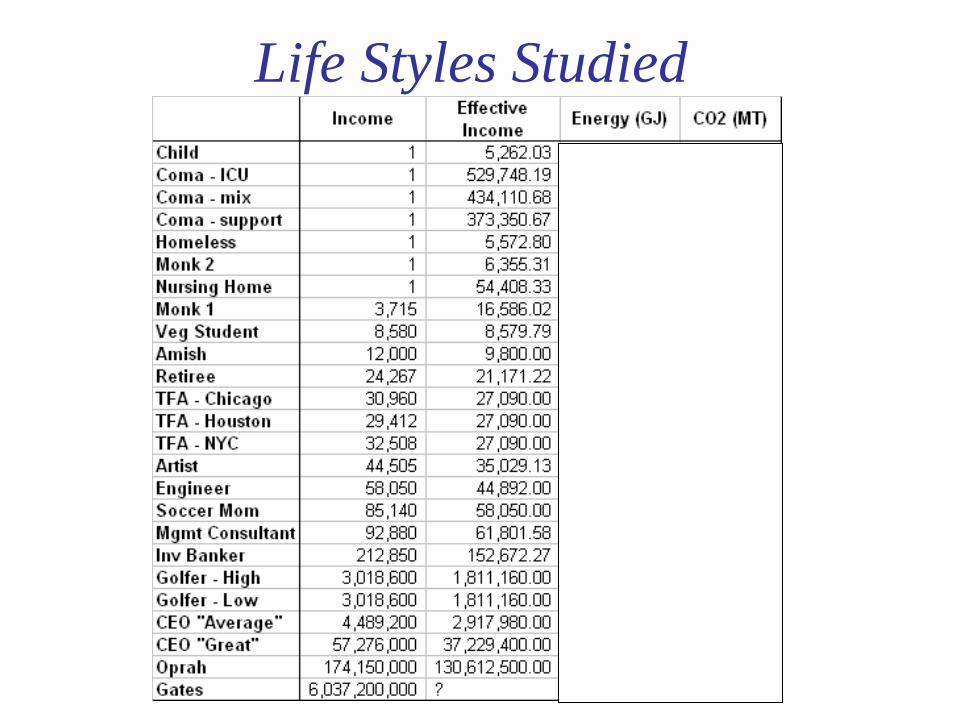
Life Styles Studied
Allocation Issues
• expenditures = income - taxes – support paid out + subsidies received
• what goods and services are bought?
• note expenditures by the 8 categories
• physical quantities, gasoline etc need to
be accounted for in the “use” phase
• Special Issues- subsidies, gifts…
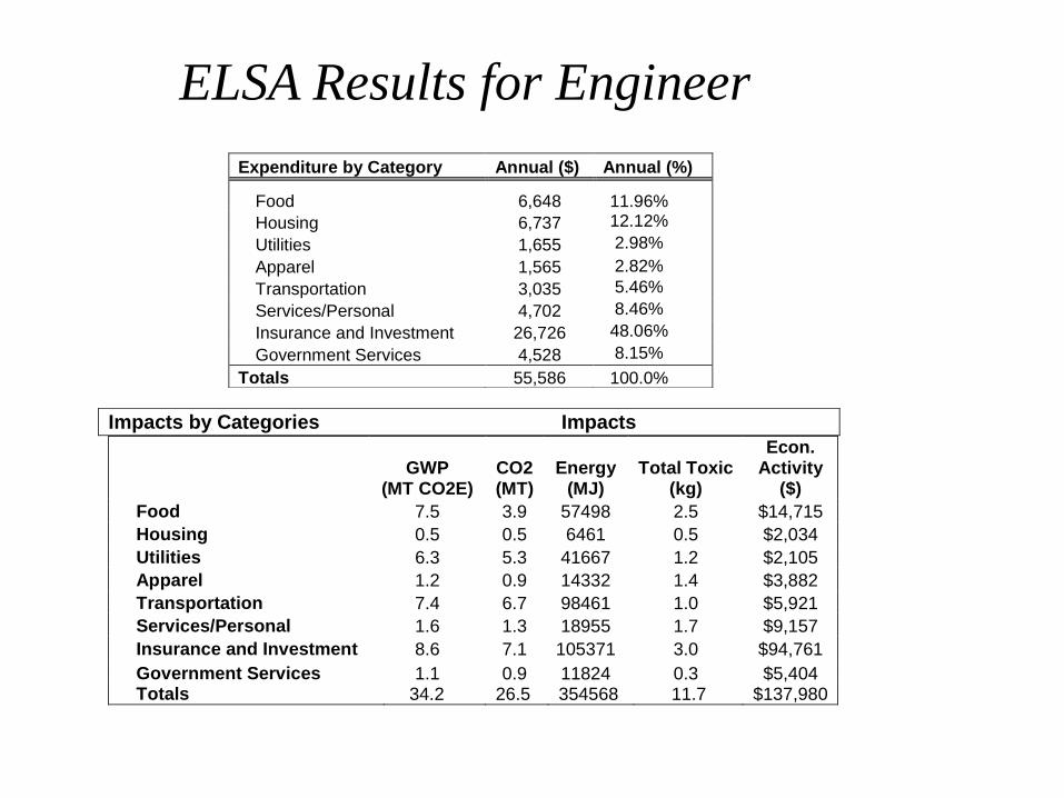
Expenditure by Category Annual ($) Annual (%)
Food 6,648
11.96%
Housing 6,737 12.12%
Utilities 1,655 2.98%
Apparel 1,565 2.82%
Transportation 3,035 5.46%
Services/Personal 4,702 8.46%
Insurance and Investment 26,726 48.06%
Government Services 4,528 8.15%
Totals 55,586 100.0%
Impacts by Categories Impacts
GWP
(MT CO2E) CO2 (MT)
Energy (MJ)
Total Toxic (kg)
Econ. Activity
($)
Food 7.5 3.9 57498 2.5 $14,715
Housing 0.5 0.5 6461 0.5 $2,034
Utilities 6.3 5.3 41667 1.2 $2,105
Apparel 1.2 0.9 14332 1.4 $3,882
Transportation 7.4 6.7 98461 1.0 $5,921
Services/Personal 1.6 1.3 18955 1.7 $9,157
Insurance and Investment 8.6 7.1 105371 3.0 $94,761
Government Services 1.1 0.9 11824 0.3 $5,404 Totals 34.2 26.5 354568 11.7 $137,980
ELSA Results for Engineer
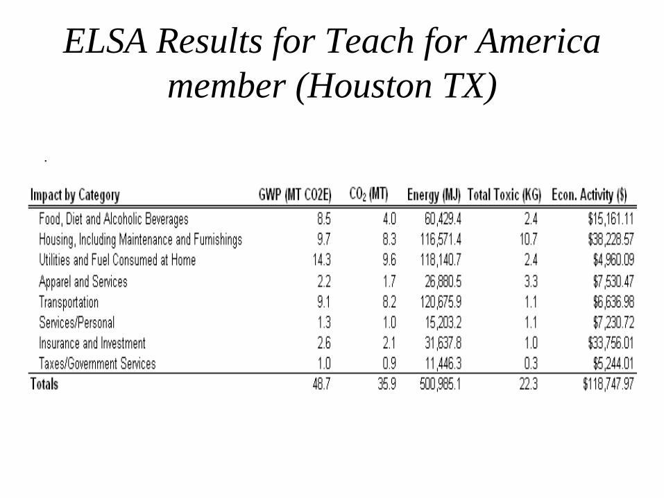
ELSA Results for Teach for America
member (Houston TX)
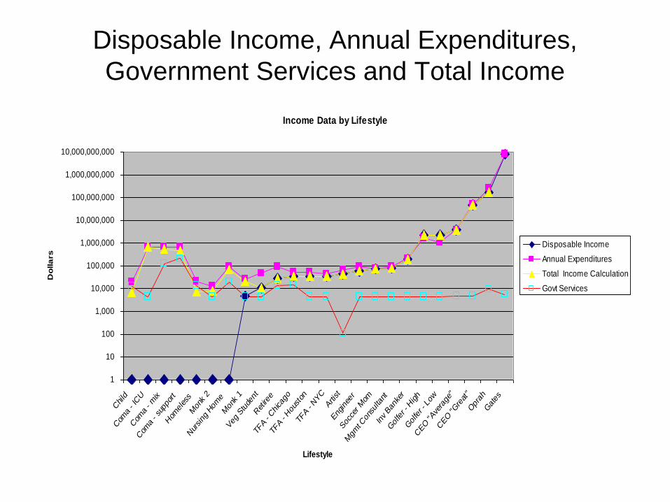
Disposable Income, Annual Expenditures,
Government Services and Total Income
Income Data by Lifestyle
1
10
100
1,000
10,000
100,000
1,000,000
10,000,000
100,000,000
1,000,000,000
10,000,000,000
Child
Com
a - IC
U
Com
a - mix
Com
a - su
pport
Hom
eles
s
Mon
k 2
Nursing
Hom
e
Mon
k 1
Veg
Stude
nt
Retire
e
TFA - Chica
go
TFA - Hou
ston
TFA - NYC
Artist
Eng
inee
r
Soc
cer Mom
Mgm
t Con
sulta
nt
Inv Ban
ker
Golfer -
High
Golfer -
Low
CEO "Ave
rage
"
CEO "Gre
at"
Opr
ah
Gates
Lifestyle
Do
lla
rs
Disposable Income
Annual Expenditures
Total Income Calculation
Govt Services
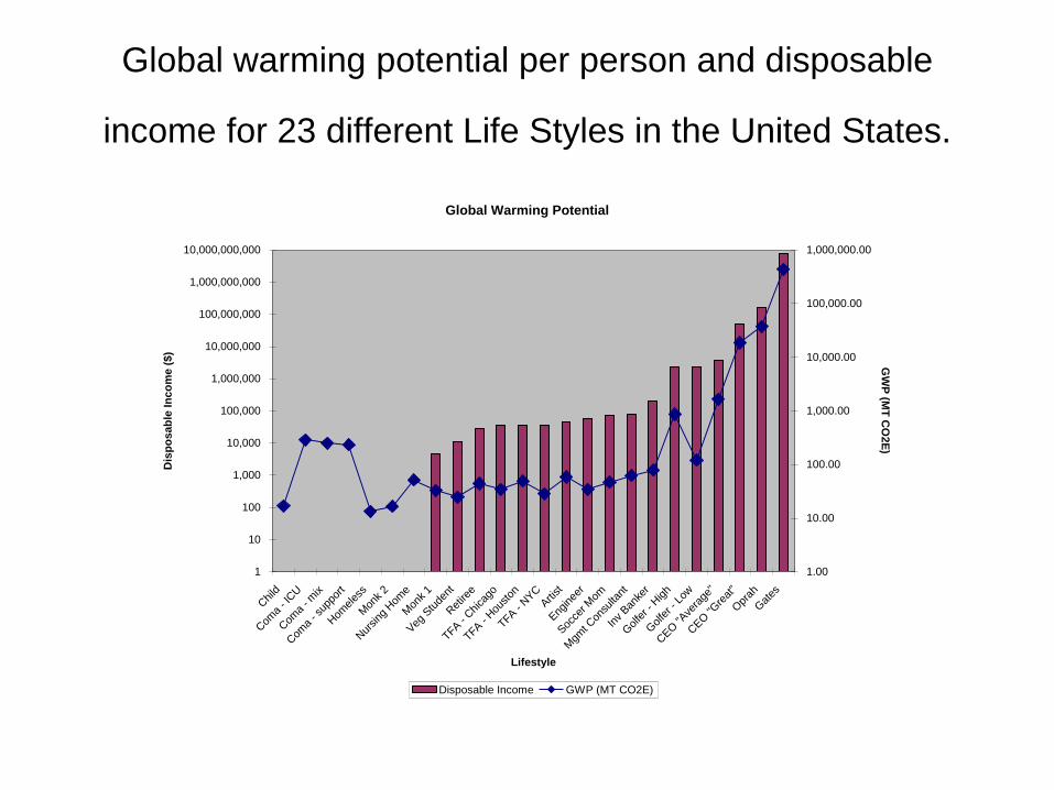
Global warming potential per person and disposable
income for 23 different Life Styles in the United States. Global Warming Potential
1
10
100
1,000
10,000
100,000
1,000,000
10,000,000
100,000,000
1,000,000,000
10,000,000,000
Child
Com
a - I
CU
Com
a - m
ix
Com
a - s
uppo
rt
Hom
eles
s
Mon
k 2
Nur
sing
Hom
e
Mon
k 1
Veg S
tude
nt
Ret
iree
TFA -
Chica
go
TFA -
Hou
ston
TFA -
NYC
Artist
Enginee
r
Socce
r Mom
Mgm
t Con
sulta
nt
Inv Ban
ker
Golfe
r - H
igh
Golfe
r - L
ow
CEO "A
vera
ge"
CEO "G
reat
"
Opr
ah
Gat
es
Lifestyle
Dis
po
sab
le In
co
me
($
)
1.00
10.00
100.00
1,000.00
10,000.00
100,000.00
1,000,000.00
GW
P (M
T C
O2
E)
Disposable Income GWP (MT CO2E)
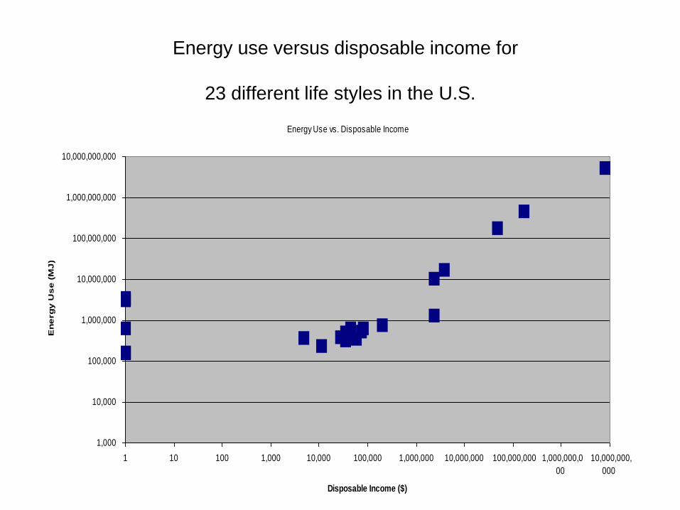
Energy use versus disposable income for
23 different life styles in the U.S. Energy Use vs. Disposable Income
1,000
10,000
100,000
1,000,000
10,000,000
100,000,000
1,000,000,000
10,000,000,000
1 10 100 1,000 10,000 100,000 1,000,000 10,000,000 100,000,000 1,000,000,0
00
10,000,000,
000
Disposable Income ($)
En
erg
y U
se
(M
J)
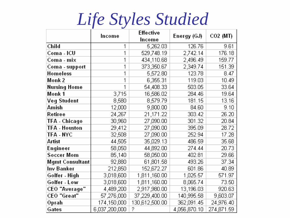
Life Styles Studied
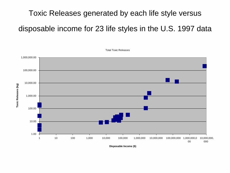
Toxic Releases generated by each life style versus
disposable income for 23 life styles in the U.S. 1997 data
Total Toxic Releases
1.00
10.00
100.00
1,000.00
10,000.00
100,000.00
1,000,000.00
1 10 100 1,000 10,000 100,000 1,000,000 10,000,000 100,000,000 1,000,000,0
00
10,000,000,
000
Disposable Income ($)
To
xic
Re
lea
se
s (
kg
)
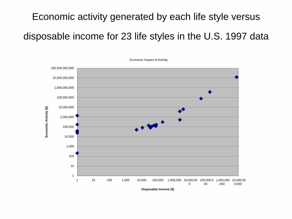
Economic activity generated by each life style versus
disposable income for 23 life styles in the U.S. 1997 data
Economic Impact of Activity
1
10
100
1,000
10,000
100,000
1,000,000
10,000,000
100,000,000
1,000,000,000
10,000,000,000
100,000,000,000
1 10 100 1,000 10,000 100,000 1,000,000 10,000,00
0
100,000,0
00
1,000,000
,000
10,000,00
0,000
Disposable Income ($)
Ec
on
om
ic A
cti
vit
y (
$)
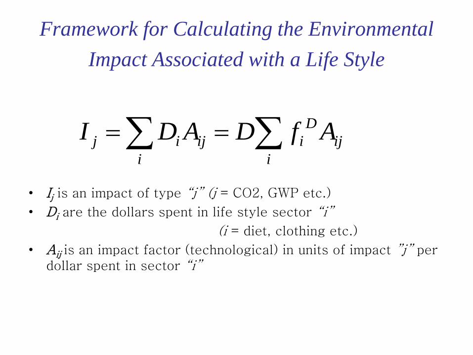
Framework for Calculating the Environmental
Impact Associated with a Life Style
• Ij is an impact of type “j” (j = CO2, GWP etc.)
• Di are the dollars spent in life style sector “i”
(i = diet, clothing etc.)
• Aij is an impact factor (technological) in units of impact ”j” per dollar spent in sector “i”
ij
i
D
iij
i
ij AfDADI
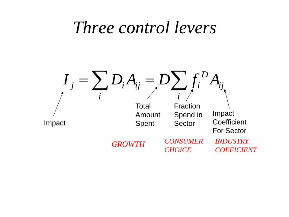
Three control levers
Impact
Total
Amount
Spent
Fraction
Spend in
Sector
Impact
Coefficient
For Sector
GROWTH CONSUMER
CHOICE INDUSTRY
COEFICIENT
ij
i
D
iij
i
ij AfDADI
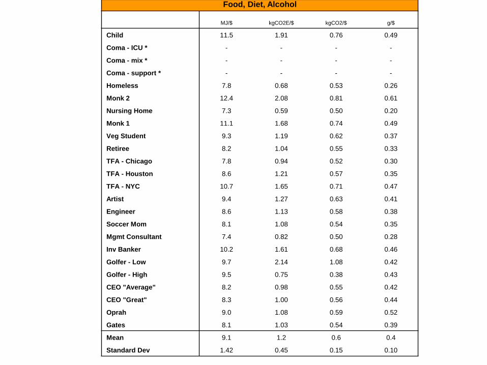
Food, Diet, Alcohol
MJ/$ kgCO2E/$ kgCO2/$ g/$
Child 11.5 1.91 0.76 0.49
Coma - ICU * - - - -
Coma - mix * - - - -
Coma - support * - - - -
Homeless 7.8 0.68 0.53 0.26
Monk 2 12.4 2.08 0.81 0.61
Nursing Home 7.3 0.59 0.50 0.20
Monk 1 11.1 1.68 0.74 0.49
Veg Student 9.3 1.19 0.62 0.37
Retiree 8.2 1.04 0.55 0.33
TFA - Chicago 7.8 0.94 0.52 0.30
TFA - Houston 8.6 1.21 0.57 0.35
TFA - NYC 10.7 1.65 0.71 0.47
Artist 9.4 1.27 0.63 0.41
Engineer 8.6 1.13 0.58 0.38
Soccer Mom 8.1 1.08 0.54 0.35
Mgmt Consultant 7.4 0.82 0.50 0.28
Inv Banker 10.2 1.61 0.68 0.46
Golfer - Low 9.7 2.14 1.08 0.42
Golfer - High 9.5 0.75 0.38 0.43
CEO "Average" 8.2 0.98 0.55 0.42
CEO "Great" 8.3 1.00 0.56 0.44
Oprah 9.0 1.08 0.59 0.52
Gates 8.1 1.03 0.54 0.39
Mean 9.1 1.2 0.6 0.4
Standard Dev 1.42 0.45 0.15 0.10
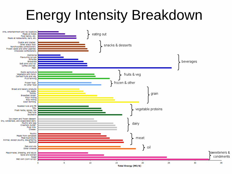
Energy Intensity Breakdown
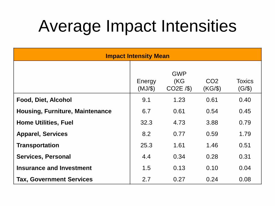
Average Impact Intensities
Impact Intensity Mean
Energy
(MJ/$)
GWP
(KG
CO2E /$)
CO2
(KG/$)
Toxics
(G/$)
Food, Diet, Alcohol 9.1 1.23 0.61 0.40
Housing, Furniture, Maintenance 6.7 0.61 0.54 0.45
Home Utilities, Fuel 32.3 4.73 3.88 0.79
Apparel, Services 8.2 0.77 0.59 1.79
Transportation 25.3 1.61 1.46 0.51
Services, Personal 4.4 0.34 0.28 0.31
Insurance and Investment 1.5 0.13 0.10 0.04
Tax, Government Services 2.7 0.27 0.24 0.08
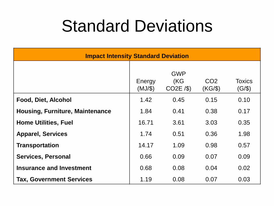
Standard Deviations
Impact Intensity Standard Deviation
Energy
(MJ/$)
GWP
(KG
CO2E /$)
CO2
(KG/$)
Toxics
(G/$)
Food, Diet, Alcohol 1.42 0.45 0.15 0.10
Housing, Furniture, Maintenance 1.84 0.41 0.38 0.17
Home Utilities, Fuel 16.71 3.61 3.03 0.35
Apparel, Services 1.74 0.51 0.36 1.98
Transportation 14.17 1.09 0.98 0.57
Services, Personal 0.66 0.09 0.07 0.09
Insurance and Investment 0.68 0.08 0.04 0.02
Tax, Government Services 1.19 0.08 0.07 0.03
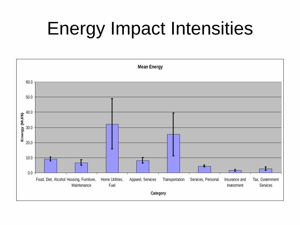
Energy Impact Intensities
Mean Energy
0.0
10.0
20.0
30.0
40.0
50.0
60.0
Food, Diet, Alcohol Housing, Furniture,
Maintenance
Home Utilities,
Fuel
Apparel, Services Transportation Services, Personal Insurance and
Investment
Tax, Government
Services
Category
En
erg
y (
MJ/$
)
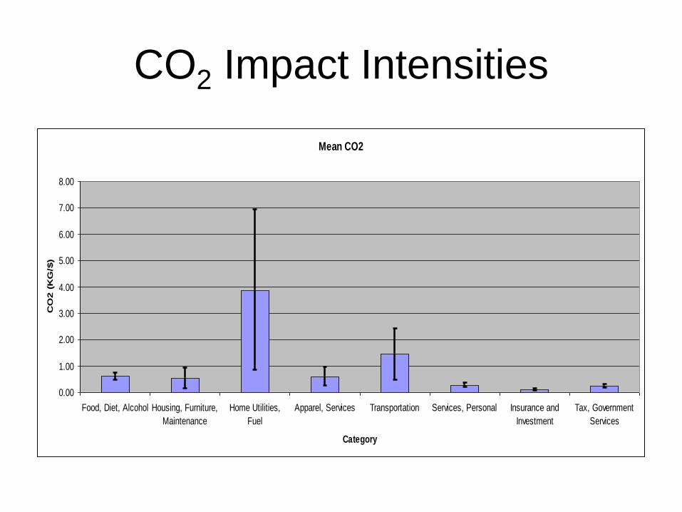
CO2 Impact Intensities
Mean CO2
0.00
1.00
2.00
3.00
4.00
5.00
6.00
7.00
8.00
Food, Diet, Alcohol Housing, Furniture,
Maintenance
Home Utilities,
Fuel
Apparel, Services Transportation Services, Personal Insurance and
Investment
Tax, Government
Services
Category
CO
2 (
KG
/$)
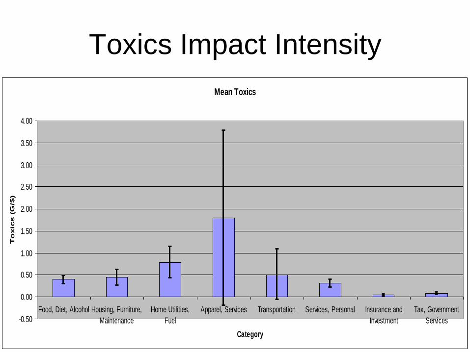
Mean Toxics
-0.50
0.00
0.50
1.00
1.50
2.00
2.50
3.00
3.50
4.00
Food, Diet, Alcohol Housing, Furniture,
Maintenance
Home Utilities,
Fuel
Apparel, Services Transportation Services, Personal Insurance and
Investment
Tax, Government
Services
Category
To
xic
s (
G/$
)
Toxics Impact Intensity
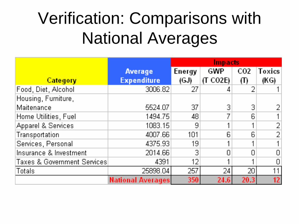
Verification: Comparisons with
National Averages
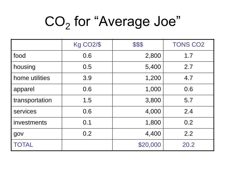
CO2 for “Average Joe”
Kg CO2/$ $$$ TONS CO2
food 0.6 2,800 1.7
housing 0.5 5,400 2.7
home utilities 3.9 1,200 4.7
apparel 0.6 1,000 0.6
transportation 1.5 3,800 5.7
services 0.6 4,000 2.4
investments 0.1 1,800 0.2
gov 0.2 4,400 2.2
TOTAL $20,000 20.2
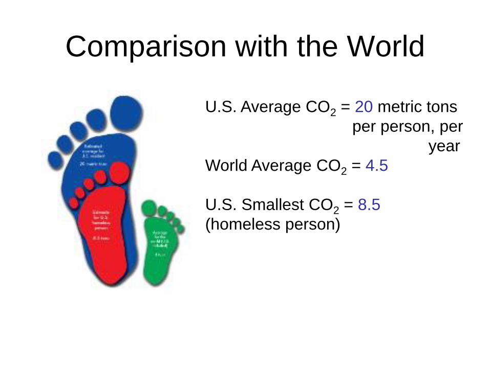
Comparison with the World
U.S. Average CO2 = 20 metric tons
per person, per
year
World Average CO2 = 4.5
U.S. Smallest CO2 = 8.5
(homeless person)
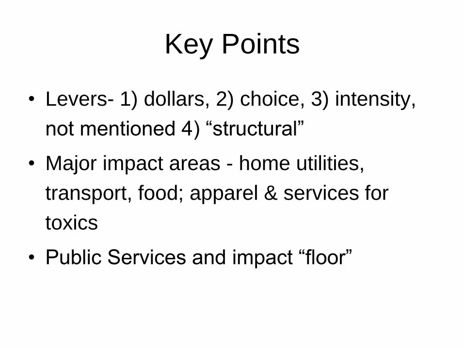
Key Points
• Levers- 1) dollars, 2) choice, 3) intensity,
not mentioned 4) “structural”
• Major impact areas - home utilities,
transport, food; apparel & services for
toxics
• Public Services and impact “floor”
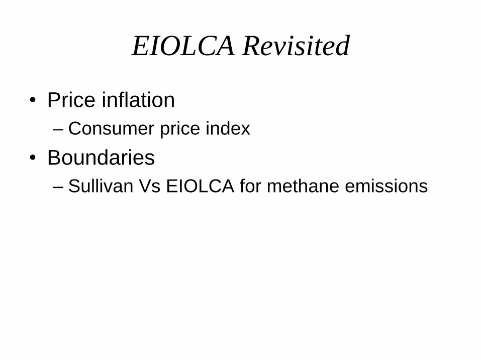
EIOLCA Revisited
• Price inflation
– Consumer price index
• Boundaries
– Sullivan Vs EIOLCA for methane emissions
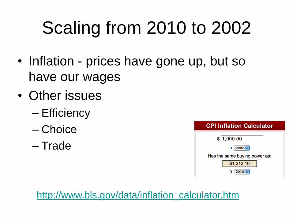
Scaling from 2010 to 2002
• Inflation - prices have gone up, but so
have our wages
• Other issues
– Efficiency
– Choice
– Trade
http://www.bls.gov/data/inflation_calculator.htm
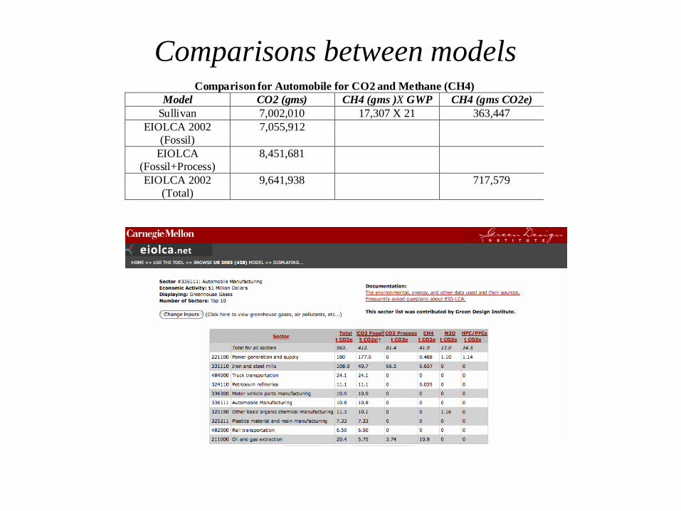
Comparisons between models Comparison for Automobile for CO2 and Methane (CH4)
Model CO2 (gms) CH4 (gms )X GWP CH4 (gms CO2e)
Sullivan 7,002,010 17,307 X 21 363,447
EIOLCA 2002
(Fossil)
7,055,912
EIOLCA
(Fossil+Process)
8,451,681
EIOLCA 2002
(Total)
9,641,938 717,579

Methane emissions ordered
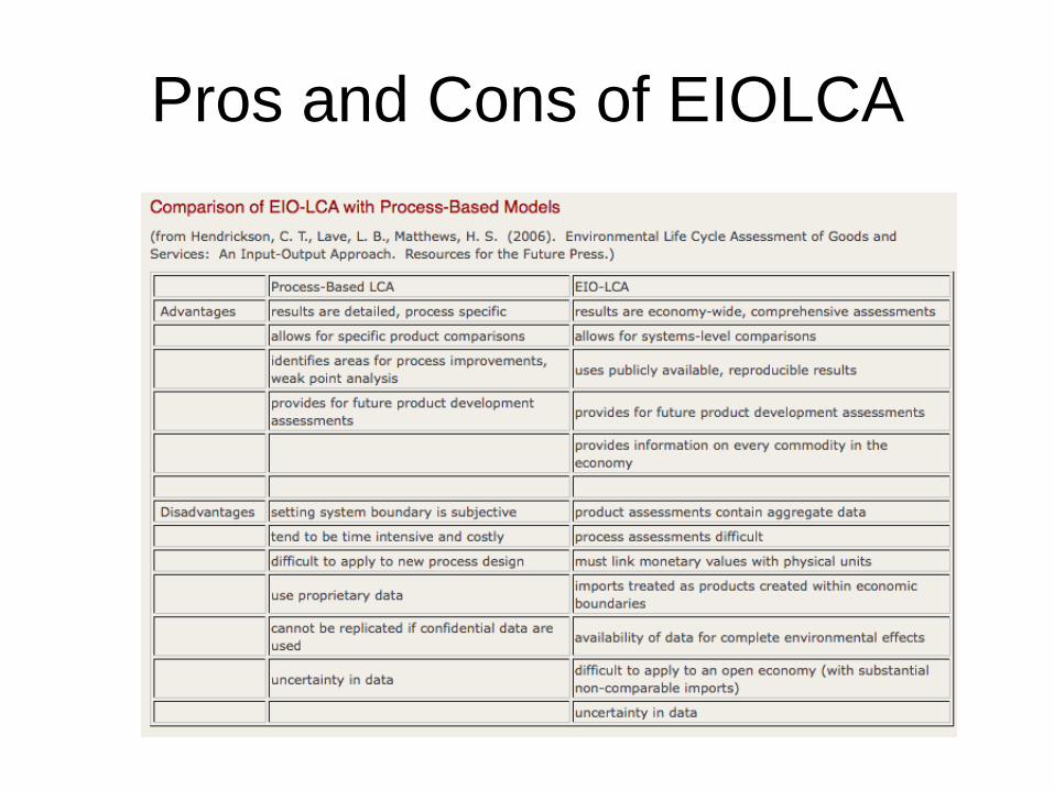
Pros and Cons of EIOLCA
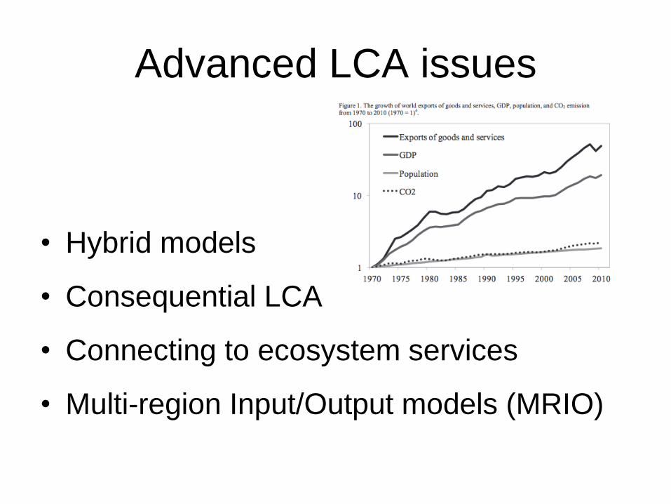
Advanced LCA issues
• Hybrid models
• Consequential LCA
• Connecting to ecosystem services
• Multi-region Input/Output models (MRIO)