Unemployment and Business Cycles

Lawrence J. ChristianoMartin EichenbaumMathias Trabandt

Disclaimer: The views expressed are those of the authors and do not necessarily reflect

those of the Board of Governors of the Federal Reserve System or any other person

associated with the Federal Reserve System.

Background

• Key challenge for modern business cycle models:— how to account for observed volatility of labor marketvariables?

• What’s the problem?— RBC, NK models without sticky wages, standard effi ciencywage models and standard DMP models all have the followingproperty:

• after an expansionary shock, wages rise rapidly and limitexpansion in employment.

— see, e.g., Alexopoulos (2004), Chetty et al (2012), Shimer(2005).

Ongoing Efforts

• New Keynesian DSGE models successful in matching time seriesdata, including hours worked, employment and real wages.

— but, they do so with the assumption that wages areexogenously sticky.

• Hall (2005) recently explained how to rationalize sticky wagesas an outcome of bargaining in a DMP-type labor market.

— idea is that bargaining set is wide enough and fluctuates littleenough to encompass sticky wage.

— GT and GST showed idea works when boundaries of bargainingset are based on aggregate data.

— but, seems unlikely to work when calibrated on more volatilemicro firm data.

Recent Development

• A basic vision about wage negotiations (Hall-Milgrom):

— once workers and firms sit down to bargain over terms, theinitial information already indicates that they are suitable foreach other.

— bargaining workers and firms are unlikely to quit negotiationsand abandon surplus, so

• wage insulated from general economic conditions.

What we do

• Work with an New Keynesian model.

• Key features of labor market:

— Wage determined by alternating offer bargaining (Binmore, etal (1986); Hall-Milgrom).

— To meet workers, firms face hiring costs, not search costs thatincrease with labor market tightness (GT, GST).

• Motivation: Yashiv (2000), Carlsson, et al (2006), Cheremukhinand Restrepo-Echavarria (2010), Lechthaler et al.(2010),Christiano-Trabandt-Walentin (2011), Furlanetto-Groshenny(2012a,b).

Result

• the NK model with the labor market modifications can -without exogenously sticky wages - account for observedcyclical properties of:

— employment, unemployment, job finding and vacancies.— standard macroeconomic variables.

• potentially removes a major criticism of New Keynesian models.

• important empirical question:

— does the vision of bargaining in the model resemble whatactually happens?

— requires survey evidence that we do not study here.

Outline

• Our model of the labor market.

• Putting the labor market into a simple macroeconomic model.

• Estimating a medium-sized DSGE model with our labor marketenvironment.

Model of the Labor Market

• Large number of identical and competitive firms; producehomogeneous output using only labor, lt.

• Firms pay fixed cost, κ, to meet a worker.• Once a worker and firm meet, they engage in alternating offerbargaining within the period over current wage.

— they take the outcome of any future bargaining as given.

• Once agreement is reached, worker begins productionimmediately.

• Job continues in next period with probability ρ.• Bargaining occurs between two types of workers and firms:

— Those that just met for the first time.— Those that reached an agreement in the previous period andwhose match survived.

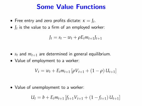
Some Value Functions

• Free entry and zero profits dictate: κ = Jt.• Jt is the value to a firm of an employed worker:

Jt = st −wt + ρEtmt+1Jt+1

• st and mt+1 are determined in general equilibrium.• Value of employment to a worker:

Vt = wt + Etmt+1 [ρVt+1 + (1− ρ)Ut+1]

• Value of unemployment to a worker:

Ut = b+ Etmt+1 [ft+1Vt+1 + (1− ft+1)Ut+1]

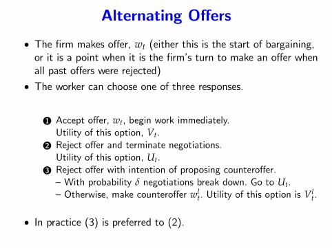
Alternating Offers

• The firm makes offer, wt (either this is the start of bargaining,or it is a point when it is the firm’s turn to make an offer whenall past offers were rejected)

• The worker can choose one of three responses.

1 Accept offer, wt, begin work immediately.Utility of this option, Vt.

2 Reject offer and terminate negotiations.Utility of this option, Ut.

3 Reject offer with intention of proposing counteroffer.—With probability δ negotiations break down. Go to Ut.—Otherwise, make counteroffer wl

t. Utility of this option is Vlt.

• In practice (3) is preferred to (2).

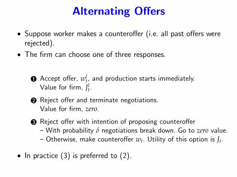
Alternating Offers

• Suppose worker makes a counteroffer (i.e. all past offers wererejected).

• The firm can choose one of three responses.

1 Accept offer, wlt, and production starts immediately.

Value for firm, Jlt.

2 Reject offer and terminate negotiations.Value for firm, zero.

3 Reject offer with intention of proposing counteroffer—With probability δ negotiations break down. Go to zero value.—Otherwise, make counteroffer wt. Utility of this option is Jt.

• In practice (3) is preferred to (2).

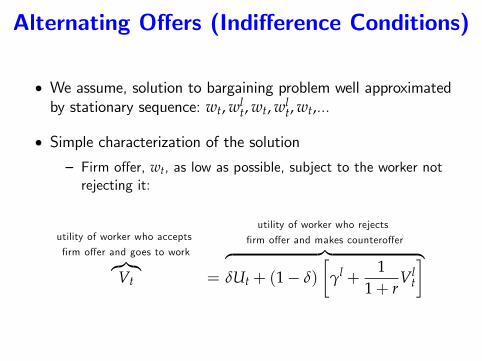
Alternating Offers (Indifference Conditions)

• We assume, solution to bargaining problem well approximatedby stationary sequence: wt, wl

t, wt, wlt, wt,...

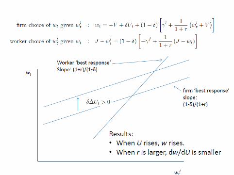
• Simple characterization of the solution— Firm offer, wt, as low as possible, subject to the worker notrejecting it:

utility of worker who accepts

firm offer and goes to work︷︸︸︷Vt =

utility of worker who rejects

firm offer and makes counteroffer︷ ︸︸ ︷δUt + (1− δ)

[γl +

11+ r

Vlt

]

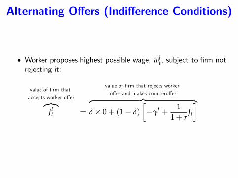
Alternating Offers (Indifference Conditions)

• Worker proposes highest possible wage, wlt, subject to firm not

rejecting it:

value of firm that

accepts worker offer︷︸︸︷Jlt =

value of firm that rejects worker

offer and makes counteroffer︷ ︸︸ ︷δ× 0+ (1− δ)

[−γf +

11+ r

Jt

]

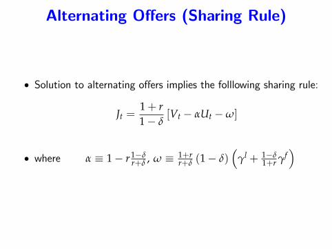
Alternating Offers (Sharing Rule)

• Solution to alternating offers implies the folllowing sharing rule:

Jt =1+ r1− δ

[Vt − αUt −ω]

• where α ≡ 1− r1−δr+δ , ω ≡ 1+r

r+δ (1− δ)(

γl + 1−δ1+r γf

)

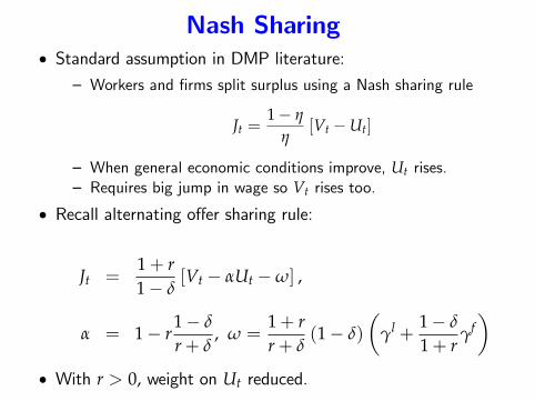
Nash Sharing• Standard assumption in DMP literature:

— Workers and firms split surplus using a Nash sharing rule

Jt =1− η

η[Vt −Ut]

— When general economic conditions improve, Ut rises.— Requires big jump in wage so Vt rises too.

• Recall alternating offer sharing rule:

Jt =1+ r1− δ

[Vt − αUt −ω] ,

α = 1− r1− δ

r+ δ, ω =

1+ rr+ δ

(1− δ)

(γl +

1− δ

1+ rγf)

• With r > 0, weight on Ut reduced.

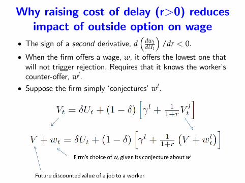
Why raising cost of delay (r>0) reducesimpact of outside option on wage

• The sign of a second derivative, d(

dwtdUt

)/dr < 0.

• When the firm offers a wage, w, it offers the lowest one thatwill not trigger rejection. Requires that it knows the worker’scounter-offer, wl.

• Suppose the firm simply ‘conjectures’wl.

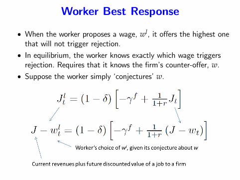
Worker Best Response

• When the worker proposes a wage, wl, it offers the highest onethat will not trigger rejection.

• In equilibrium, the worker knows exactly which wage triggersrejection. Requires that it knows the firm’s counter-offer, w.

• Suppose the worker simply ‘conjectures’w.

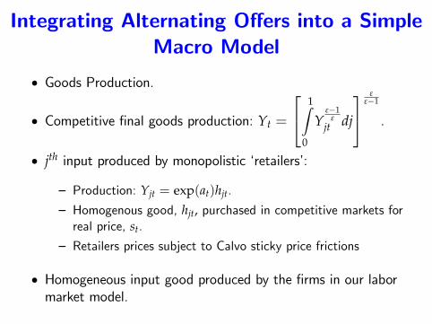
Integrating Alternating Offers into a SimpleMacro Model

• Goods Production.

• Competitive final goods production: Yt =

1∫0

Yε−1

εjt dj

εε−1

.

• jth input produced by monopolistic ‘retailers’:

— Production: Yjt = exp(at)hjt.

— Homogenous good, hjt, purchased in competitive markets forreal price, st.

— Retailers prices subject to Calvo sticky price frictions

• Homogeneous input good produced by the firms in our labormarket model.

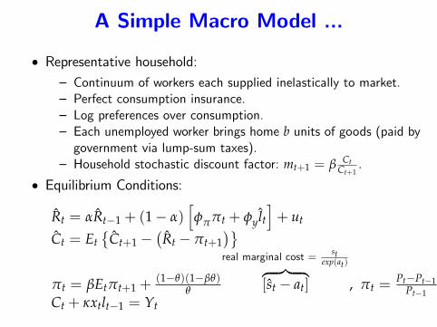
A Simple Macro Model ...

• Representative household:— Continuum of workers each supplied inelastically to market.— Perfect consumption insurance.— Log preferences over consumption.— Each unemployed worker brings home b units of goods (paid bygovernment via lump-sum taxes).

— Household stochastic discount factor: mt+1 = β CtCt+1

.

• Equilibrium Conditions:

Rt = αRt−1 + (1− α)[φππt + φylt

]+ ut

Ct = Et{

Ct+1 −(Rt − πt+1

)}πt = βEtπt+1 +

(1−θ)(1−βθ)θ

real marginal cost = stexp(at)︷ ︸︸ ︷

[st − at] , πt =Pt−Pt−1

Pt−1Ct + κxtlt−1 = Yt

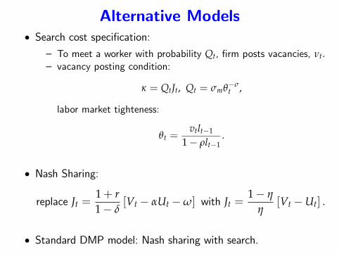
Alternative Models• Search cost specification:

— To meet a worker with probability Qt, firm posts vacancies, νt.— vacancy posting condition:

κ = QtJt, Qt = σmθ−σt ,

labor market tighteness:

θt =vtlt−1

1− ρlt−1.

• Nash Sharing:

replace Jt =1+ r1− δ

[Vt − αUt −ω] with Jt =1− η

η[Vt −Ut] .

• Standard DMP model: Nash sharing with search.

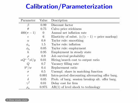
Calibration/Parameterization0.1.5 Small Model: Calibrated Parameters

Table 1: Calibrated Parameters in the Small Model

Parameter Value Description

0.99 Discount factor

0.75 Calvo price stickiness

400( 1) 0 Annual net ináation rate

6 Elasticity of subst. (=( 1) = price markup) 0.8 Taylor rule: smoothing

1.5 Taylor rule: ináation

h 0.05 Taylor rule: employment

h 0.95 Employment in steady state

0.9 Job survival probability

Q1xl=y 0.01 Hiring/search cost to output ratio

Q 0.7 Vacancy Ölling rate

bu=w 0.4 Replacement ratio

0.5 Unempl. share in matching function

r 0.001 Intra-period discounting alternating o§er barg.

0.05 Prob. of barg. session breakup alt. o§er barg.

f 0.01 Delay cost for Örm

a 0.975 AR(1) of level shock to technology

1 Inverse labor supply elast. (EHL/CGG)

w 0.75 Calvo wage stickiness (EHL)

w 6 Elasticity (w=(w 1) = EHL wage markup)

0.1.6 Small Model: Implied Steady States

Table 2: Small Model Steady States and Implied Parameters

VariableAlt.O§er and Nash

Unemp. Models

CGG/EHL

ModelsDescription

C 0.941 0.95 Consumption

ea 1 1 Steady state technology

w 0.989 1 Market wage

wl 1.004 - Countero§er wage (alt. o§er barg.)

U 90.37 - Value of unemployment

V 91.15 - Value of worker at market wage

V l 91.17 - Value of worker at countero§er wage (alt.o§er barg.)

J 0.1 - Firm value at market wage

J l 0.085 - Firm value at worker countero§er wage (alt.o§er barg.)

u 0.05 - Steady state unemployment rate

f 0.655 - Job Önding rate

0.936 - Labor market tightness, v=(1 h)m 0.677 - Level parameter in matching function

! -2.499 - Parameter in alternating o§er barg. sharing rule

l -0.118 - Worker beneÖt while not working after rejecting o§er

bu 0.396 - Unemployment beneÖts

0.887 - Worker surplus share: (V U)=(V U + J) 0.1 (0.07) - Hiring (search) cost parameter

5

Show steady state

0 1 2 3 4 5

10

20

30

40

Inflation rate (ABP)

0 1 2 3 4 5

0.05

0.1

0.15

0.2

Real consumption (%)

0 1 2 3 4 5

−0.2

−0.15

−0.1

−0.05

Unemployment rate (p.p.)

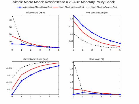
Simple Macro Model: Responses to a 25 ABP Monetary Policy Shock

0 1 2 3 4 5

0.2

0.4

0.6

0.8

1Real wage (%)

Alternating Offers/Hiring Cost Nash Sharing/Hiring Cost Nash Sharing/Search Cost

0 1 2 3 4 5

10

20

30

40

Inflation rate (ABP)

0 1 2 3 4 5

0.05

0.1

0.15

0.2

Real consumption (%)

0 1 2 3 4 5

0.05

0.1

0.15

0.2

Hours (%)

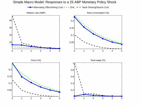
Simple Macro Model: Responses to a 25 ABP Monetary Policy Shock

0 1 2 3 4 5

0.2

0.4

0.6

0.8

1Real wage (%)

Alternating Offers/Hiring Cost EHL Nash Sharing/Search Cost

0 10 20 30

−80

−70

−60

−50

−40

−30

−20

−10

Inflation rate (ABP)

0 10 20 30

0.6

0.8

1

1.2

1.4

1.6

Real consumption (%)

0 10 20 30

−0.7

−0.6

−0.5

−0.4

−0.3

−0.2

−0.1

0Unemployment rate (p.p.)

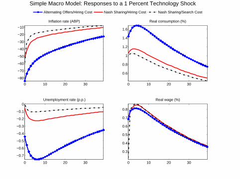
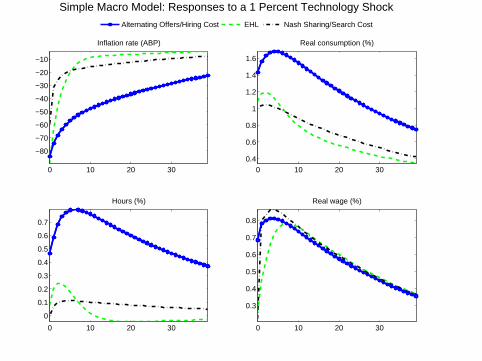
Simple Macro Model: Responses to a 1 Percent Technology Shock

0 10 20 30

0.3

0.4

0.5

0.6

0.7

0.8

Real wage (%)

Alternating Offers/Hiring Cost Nash Sharing/Hiring Cost Nash Sharing/Search Cost

0 10 20 30

−80

−70

−60

−50

−40

−30

−20

−10

Inflation rate (ABP)

0 10 20 300.4

0.6

0.8

1

1.2

1.4

1.6

Real consumption (%)

0 10 20 30

0

0.1

0.2

0.3

0.4

0.5

0.6

0.7

Hours (%)

Simple Macro Model: Responses to a 1 Percent Technology Shock

0 10 20 30

0.3

0.4

0.5

0.6

0.7

0.8

Real wage (%)

Alternating Offers/Hiring Cost EHL Nash Sharing/Search Cost

Simple Macro Model Implications

• Alternating offers and hiring costs perform roughly same assticky wages.

• Next, evaluate quantitative implications of our labor marketmodel in context of estimated medium-sized DSGE model.

Medium-Sized DSGE Model

• Standard empirical NK model (e.g., CEE, ACEL, SW).

— Habit persistence in preferences.

— Variable capital utilization.

— Investment adjustment costs.

• Our labor market structure

Medium-Sized DSGE Model

• Estimate VAR impulse responses of aggregate variables toCEE-type monetary policy shock.

• 11 variables considered:— Macro variables and real wage, hours worked, unemployment,job finding rate, vacancies.

• Impulse-response matching by Bayesian methods.

0 5 10 15−0.2

0

0.2

0.4

GDP

0 5 10 15

−0.1

0

0.1

0.2

Inflation

0 5 10 15

−0.6

−0.4

−0.2

0

0.2Federal Funds Rate

0 5 10 15

0

0.5

1Capacity Utilization

0 5 10 15

−0.1

0

0.1

0.2

0.3

Hours

0 5 10 15

−0.15

−0.1

−0.05

0

0.05

Wage

0 5 10 15−0.1

0

0.1

0.2

Consumption

0 5 10 15

−0.5

0

0.5

1

Investment

0 5 10 15−0.2

−0.1

0

Unempl. Rate

0 5 10 15

0

2

4

Vacancies

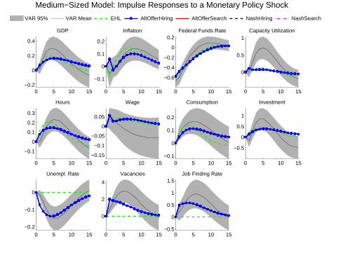
Medium−Sized Model: Impulse Responses to a Monetary Policy Shock

0 5 10 15−0.5

0

0.5

1

1.5Job Finding Rate

VAR 95% VAR Mean EHL AltOfferHiring AltOfferSearch NashHiring NashSearch

Conclusion• We constructed a model that accounts for the key features ofthe monetary transmission mechanism:— for inflation and aggregate macro variables (includingunemployment, vacancies and labor market flows).

• Our preferred model has two key features:1 Wages determined by alternative offer protocol.2 Firms face hiring rather than search costs.

• Nominal wages are inertial, but not by assumption.

• Currently studying whether medium sized model can replicateestimated responses to technology shocks.— results with simple model suggests it can.

• Question: which policy implications of existing DSGE modelsare sensitive to our labor market structure?