LAURENTIAN GREAT LAKES DOUBLE-CO, CLIMATE … · LAURENTIAN GREAT LAKES DOUBLE-CO, CLIMATE CHANGE HYDROLOGICAL IMPACTS ' ... supplies during the late fall and winter months I' when

LAURENTIAN GREAT LAKES DOUBLE-CO,

CLIMATE CHANGE HYDROLOGICAL IMPACTS '

T H O M A S E. C R O L E Y I1 - Great Lakes Environmental Research Laboratoty, National Oceanic and Atmospheric Admini~,tration,

2205 Commonwealth Blvd., Ann Arbor, MI 48105, U.S.A.

I

1 Abstract. The Great Lakes Environmental Research Laboratory has developed conceptual daily models for simulating moisture storages in and runoff from the 121 watersheds draining into the Laurentian Great Lakes, over-lake precipitation into each lake, and the heat storages in and evaporation from each lake. We combine these components as net basin supplies for each lake to consider climate change scenarios developed from atmospheric general circulation models (GCMs). Recent scenarios of a doubling of atmospheric CO,, available from the Goddard Institute for Space Studies, the Geophysical Fluid Dynamics Labora- tory, and Oregon State University are considered by making changes in historical meteorological data similar to the changes observed in the GCMs, observing the impact of the changed data in the model outputs, and comparing outputs to model results using unchanged data, representing comparison to an unchanged atmosphere. This study indicates a 23 to 5l0/0 reduction in net basin supplies to all the Great Lakes; there is significant variation in the components of these supplies among the three GCMs. The basins various moisture storages become dryer and the lakes are warmer with associated hydrological impacts.

1. Introduction

Some past estimates of climate change impacts considered independent cha~ges to meteorological variables to assess hydrological model output changes. Quinn and Croley (1983) estimated that a 3 "C rise in air temperature coupled with a 6.5% increase in precipitation would decrease the net basin supply (runoff and over-lake precipitation less lake evaporation) to Lake Superior by 10%; with no precipiiation increase, this temperature rise was estimated to decrease the Lake Erie net basin supply by 33%. To consider consistent dependent changes among meteorological variables, the U.S. Environmental Protection Agency (USEPA, 1984) and Rind (personal communication, 1988) used the hydrologic components of general circulation models (GCMs) of the earths atmosphere to assess changes in water availability in several regions throughout North America, but the regions were very large. Rind used only four regions for the entire continent and indicated that assessments with smaller regions were needed.

1 By linking regional hydrological models with GCMs, we can better assess regional changes associated with climate change. Cohen (1986) modified Goddard Institute for Space Studies (GISS) double-CO, (-2 x CO,) GCM scenarios and

' GLERL Contribution NO. 646.

Climatic Change 17: 2747.1990. O 1990 Kluwer Academic Publishers. Printed in the Netherlands.

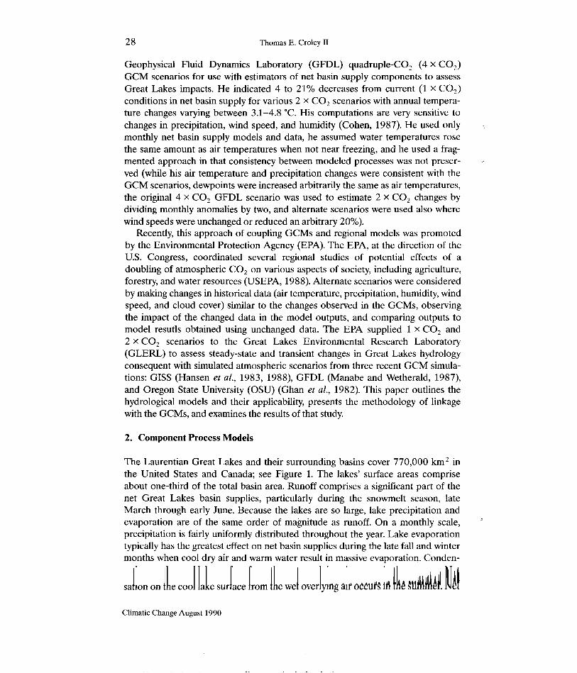
2 8 Thomas E. Croley I1

Geophysical Fluid Dynamics Laboratory (GFDL) quadruple-CO, (4 X CO,) GCM scenarios for use with estimators of net basin supply components to assess Great Lakes impacts. He indicated 4 to 21°h decreases from current (1 x CO,) conditions in net basin supply for various 2 X CO, scenarios with annual temperature changes varying between 3.1-4.8 "C. His computations are very sensitive to changes in precipitation, wind speed, and humidity (Cohen, 1987). He used only monthly net basin supply models and data, he assumed water temperatures rose the same amount as air temperatures when not near freezing, and he used a frag- mented approach in that consistency between modeled processes was not preserved (while his air temperature and precipitation changes were consistent with the GCM scenarios, dewpoints were increased arbitrarily the same as air temperatures, the original 4 x CO, GFDL scenario was used to estimate 2 x CO, changes by dividing monthly anomalies by two, and alternate scenarios were used also where wind speeds were unchanged or reduced an arbitrary 20%).

Recently, this approach of coupling GCMs and regional models was promoted by the Environmental Protection Agency (EPA). The EPA, at the direction of the U.S. Congress,. coordinated several regional studies of potential effects of a doubling of atmospheric CO, on various aspects of society, including agriculture, forestry, and water resources (USEPA, 1988). Alternate scenarios were considered by making changes in historical data (air temperature, precipitation, humidity, wind speed, and cloud cover) similar to the changes observed in the GCMs, observing the impact of the changed data in the model outputs, and comparing outputs to model resutls obtained using unchanged data. The EPA supplied 1 X CO, and 2 X CO, scenarios to the Great Lakes Environmental Research Laboratory (GLERL) to assess steady-state and transient changes in Great Lakes hydrology consequent with simulated atmospheric scenarios from three recent GCM simulations: GISS (Hansen et al., 1983, 1988), GFDL (Manabe and Wetherald, 1987), and Oregon State University (OSU) (Ghan et al., 1982). This paper outlines the hydrological models and their applicability, presents the methodology of linkage with the GCMs, and examines the results of that study.

2. Component Process Models

The Laurentian Great Lakes and their surrounding basins cover 770,000 km2 in the United States and Canada; see Figure 1. The lakes' surface areas comprise about one-third of the total basin area. Runoff comprises a significant part of the net Great Lakes basin supplies, particularly during the snowmelt season, late March through early June. Because the lakes are so large, lake precipitation and evaporation are of the same order of magnitude as runoff. On a monthly scale,

-

precipitation is fairly uniformly distributed throughout the year. Lake evaporation typically has the greatest effect on net basin supplies during the late fall and winter months when cool dry air and warm water result in massive evaporation. Conden-

I' Ib I I k d ~ U I I " . I! &/. NL! sa Ion on e coo a e su ace rom e we over y~ng all OCCUYS lfi B BU~H Climatic Change August 1990

Laurentian Great Lakes Double-CO, 2 9

- -. --

Fig. 1. Location map for the Laurentian Great Lakes.

groundwater flows to each of the Great Lakes are generally negligible. Net basin supplies typically reach a maximum in the late spring and a minimum in late fall.

As water temperatures generally peak in August (September for Superior) at 15 to 25 "C and drop to freezing or near-freezing during the winter, the water column in each lake 'turns over' (deep lower-density waters rise and mix with heavier surface layers) twice a year as surface temperature passes through that of maximum density for water (about 4 "C). There is also extensive ice cover on most of the lakes during most winters. The large heat storage of the deep lakes forestalls and reduces ice formation as well as shifting the large evaporation response to fall and winter.

The Great Lakes Environmental Research Laboratory has developed conceptual model-based techniques for simulating moisture storages and runoff from the watersheds draining into the Great Lakes, over-lake precipitation into each of the Great Lakes and Lake St. Clair (hereafter included as a Great Lake), and the heat storages and evaporation from each of the lakes. We model each of these components separately and combine them to estimate net basin supplies to Lakes Supe- rior, Michigan, Huron, St. Clair, Erie, and Ontario for simulating the existing basin and lake storages of water and heat in response to possible meteorology. Integration of the models allows the consideration of climate change scenarios developed from GCMs through links with air temperature, precipitation, humidity, wind speed, and cloud cover.

Climatic Change August 1990

30 Thomas E. Croley I1

TABLE I: Large basin runoff model calibration statisticsa

Lake

Superior Michigan Huron St. Clair Erie Ontario

Number of sub-basins

Mean l-day flow (rnm)

1.12 0.89 1.06 0.90 1.01 1.41

Flow std. dev. (rnm)

0.67 0.47 0.69 1.36 1.28 1.13

Root mean square error (mm)

0.25 0.18 0.26 0.62 0.54 0.43

Correlation

Calib. Verif.

0.93 0.77 0.93 0.86 0.92 0.69 0.89 0.87 0.9 1 0.90 0.93 0.89

" Calibrations and statistics generally cover 1966-83; verification correlation generally covers 1956-63.

Equivalent depth over the land portion of the basin.

The GLERL Large Basin Runoff Model (LBRM) uses daily precjpitation, temperature, and insolation (the latter available from climatological summaries as a func- tion of location) to determine snowpack accumulations and degree-day calculation of snowmelt (Croley, 1983a, b). The net surface supply is divided into infiltration and channel inflow by assuming infiltration to be proportional to the net surface supply rate and to the unsaturated surface area. Infiltration enters a cascade of moisture storages within the basin and outflow from each storage is proportional to the storage amount. Evapotranspiration also is proportional to available moisture but additionally to the available heat; it also reduces the heat available for subse- quent evapotranspiration. Mass continuity yields a first-order linear differential equation for each of the moisture storages (Croley, 1982) which are solved simulta- neously to determine daily moisture storage, evapotranspiration, and basin runoff.

The Great Lakes basin is divided into 121 watersheds, each draining directly to a lake, grouped into the six lake basins. The meteorologic data from over 1800 stations about and in the watersheds are combined through Thiessen weighting to produce areally-averaged daily time series of precipitation and maximum and minimum air temperatures for each watershed (Croley and Hartmann, 1985b). Records for all 'most-downstream' flow stations are combined by aggregating and extra- polating for ungauged areas to estimate the daily runoff to the lake from each watershed. The LBRM was calibrated generally over 1965-82 to minimize the sum-of-squared-errors between model and actual daily flow volumes for each watershed (Croley, 1983b; Croley and Hartmann, 1984, 1985a). Table I presents calibration statistics for lake-basin groupings of the watersheds as well as independent verification correlations for 1956-63. The latter are a little lower than the calibration correlations but quite good except for Lakes Superior and Huron (there were less than two thirds as many flow gages available for 1956-63 as for the calibration period for these basins). The LBRM was also used in forecasts of Lake Superior water levels (Croley and Hartmann, 1987) and comparisons with climatic


Laurentian Great Lakes Double-COz 31

outlooks showed the runoff model was very close to actual runoff (monthly correlations of net basin supply were on the order of 0.99) for the period August 1982- December 1984 which is outside of and wetter than the calibration period (Croley and Hartmann, 1986).

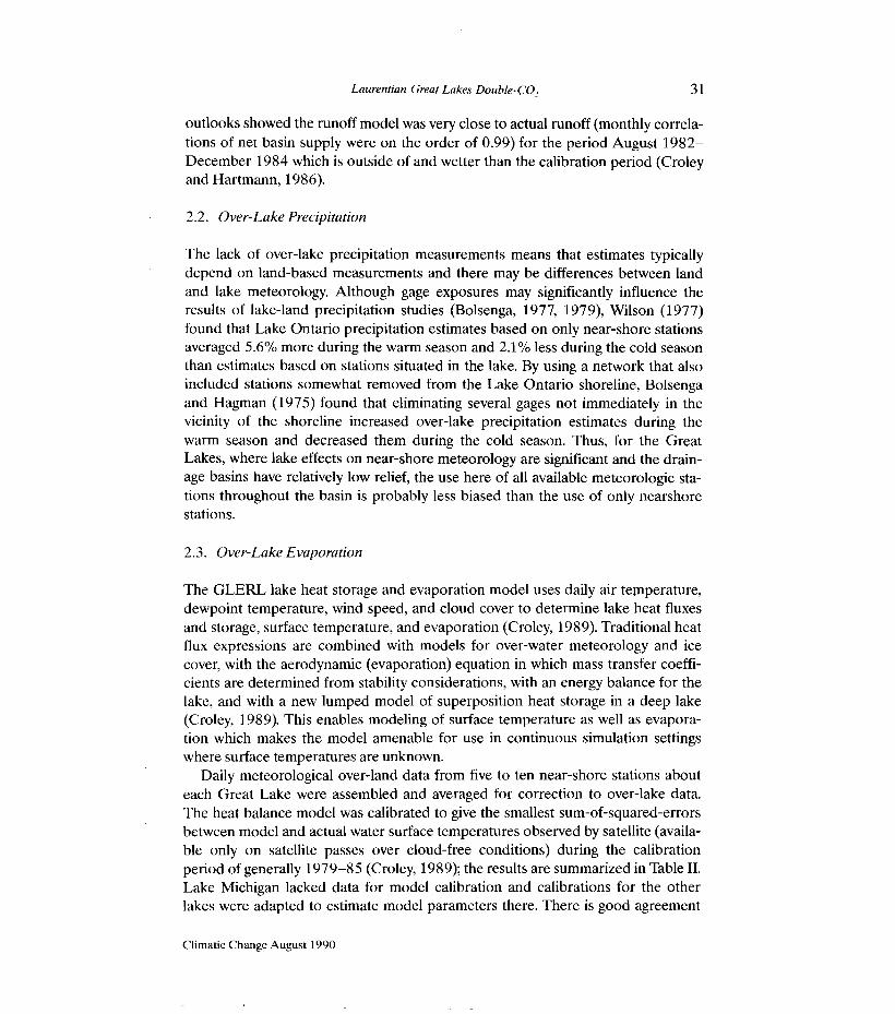
2.2. Over-Lake Precipitation

The lack of over-lake precipitation measurements means that estimates typically depend on land-based measurements and there may be differences between land and lake meteorology. Although gage exposures may significantly influence the results of lake-land precipitation studies (Bolsenga, 1977, 1979), Wilson (1977) found that Lake Ontario precipitation estimates based on only near-shore stations averaged 5.6% more during the warm season and 2.1% less during the cold season than estimates based on stations situated in the lake. By using a network that also included stations somewhat removed from the Lake Ontario shoreline, Bolsenga and Hagman (1975) found that eliminating several gages not immediately in the vicinity of the shoreline increased over-lake precipitation estimates during the warm season and decreased them during the cold season. Thus, for the Great Lakes, where lake effects on near-shore meteorology are significant and the drain- age basins have relatively low relief, the use here of all available meteorologic stations throughout the basin is probably less biased than the use of only nearshore stations.

2.3. Over-Lake Evaporation

The GLERL lake heat storage and evaporation model uses daily air temperature, dewpoint temperature, wind speed, and cloud cover to determine lake heat fluxes and storage, surface temperature, and evaporation (Croley, 1989). Traditional heat flux expressions are combined with models for over-water meteorology and ice cover, with the aerodynamic (evaporation) equation in which mass transfer coeffi- cients are determined from stability considerations, with an energy balance for the lake, and with a new lumped model of superposition heat storage in a deep lake (Croley, 1989). This enables modeling of surface temperature as well as evaporation which makes the model amenable for use in continuous simulation settings where surface temperatures are unknown.

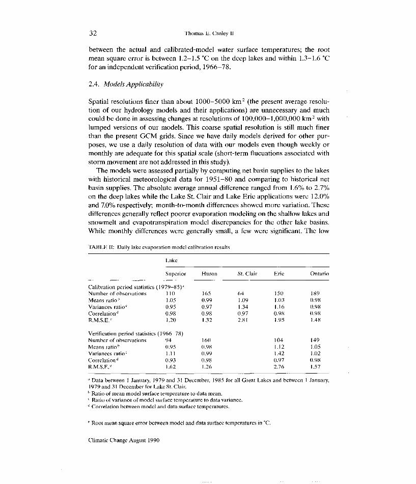
Daily meteorological over-land data from five to ten near-shore stations about each Great Lake were assembled and averaged for correction to over-lake data. The heat balance model was calibrated to give the smallest sum-of-squared-errors between model and actual water surface temperatures observed by satellite (available only on satellite passes over cloud-free conditions) during the calibration period of generally 1979-85 (Croley, 1989); the results are summarized in Table 11. Lake Michigan lacked data for model calibration and calibrations for the other lakes were adapted to estimate model parameters there. There is good agreement



between the actual and calibrated-model water surface temperatures; the root mean square error is between 1.2-1.5 "C on the deep lakes and within 1.3-1.6 "C for an independent verification period, 1966-78.

2.4. Models Applicability

Spatial resolutions finer than about 1000-5000 km2 (the present average resolution of our hydrology models and their applications) are unnecessary and much could be done in assessing changes at resolutions of 100,000-1,000,000 km2 with lumped versions of our models. This coarse spatial resolution is still much finer than the present GCM grids. Since we have daily models derived for other pur- poses, we use a daily resolution of data with our models even though weekly or monthly are adequate for this spatial scale (short-term flucuations associated with storm movement are not addressed in this study).

The models were assessed partially by computing net basin supplies to the lakes with historical meteorological data for 1951-80 and comparing to historical net basin supplies. The absolute average annual difference ranged from 1.6% to 2.7% on the deep lakes while the Lake St. Clair and Lake Erie applications were 12.0% and 7.0% respectively; month-to-month differences showed more variation. These differences generally reflect poorer evaporation modeling on the shallow lakes and snowmelt and evapotranspiration model discrepancies for the other lake basins. While monthly differences were generally small, a few were significant. The low

TABLE 11: Daily lake evaporation model calibration results

Lake --

Superior Huron St. Clair Erie Ontario

Calibration period statistics (1979-85)~' Number of observations 110 165 64 150 189 Means ratio 1.05 0.99 1.09 1.03 0.98 Variances ratioc 0.95 0.97 1.34 1.16 0.98 Correlation" 0.98 0.98 0.97 0.98 0.98 R.M.S.E.' 1.20 1.32 2.8 1 1.95 1.48

Verification period statistics (1 966-78) Number of observations 94 160 104 149 Means ratio 0.95 0.98 1.12 1.05 Variances ratio' 1.11 0.99 1.42 1.02 Correlation 0.93 0.98 0.97 0.98 R.M.S.E.' 1.62 1.26 2.76 1.57

Data between 1 Jafiuary, 1979 and 31 December, 1985 for all Great Lakes and between 1 January, 1979 and 31 December for Lake St. Clair. Ratio of mean model surface temperature to data mean. Ratio of variance of model surface temperature to data variance.

" Correlation between model and data surface temperatures.

Root mean square error between model and data surface temperatures in 'C.


Laurentian Great Lakes Double-CO, 33

annual residuals were felt to be acceptable for use of these models in assessing changes from the current climate as they would be consistently applied to both a 'present' and a 'changed' climate. Further assessment of model deficiencies with comparisons to historical net basin supplies is difficult since the latter are derived from water budgets which incorporate all budget term errors in the derived net basin supplies.

There is some indication of model applicability outside of the time periods over which the models were calibrated as indicated above and in Tables I and 11. To assess the applicability of the process models to a climate warmer than the one under which they were calibrated and verified requires access to meteorologic data and process outputs for the warmer climate which unfortunately do not exist. Warm periods early in this century are not sufficiently documented for the Great Lakes. In particular, data are lacking on watershed runoff to the lakes, water surface temperatures, wind speed, humidity, cloud cover, and solar insolation.

It is entirely possible that the models are tied somewhat to the present climate; empiricism is employed in the evapotranspiration component of the LBRM and in some of the heat flux terms in the heat balance and lake evaporation model. Cali- brations were performed under the present climate. The models are all based on physical concepts that should be good under any climate; but, the assumption is made that they represent processes under a changed climate that are the same as the present ones. However, the calibration and verification periods for the component process models include a range of air temperatures, precipitation, and other meteorological variables that encompass much of the changes in these variables predicted for a changed climate. Even though the changes are transitory in the calibration and verification period data sets, the models appear to work well under these conditions.

3. Steady-State Hydrologic Impacts

3.1. Methodology

First, we simulated 30 years of 'present' hydrology (the 'base case' or '1 x CO,' scenario) by using historical daily average, maximum, and minimum air temperatures, precipitation, wind speed, humidity, and cloud cover data for the 1951-80 period in the hydrology models. The initial conditions were arbitrarily set but an initializa- tion simulation period of 1 January, 1948 through 31 December, 1950 was used to allow the models to converge to conditions (basin moisture storages, water surface temperatures, and lake heat storages) initial to the 1 January, 1951 through 31 December, 1980 period. Then we conducted simulations with adjusted data sets.

EPA supplied ratios of 'future' to 'present7 monthly absolute air temperature, specific humidity, cloud cover, and precipitation, and differences of 'future' and 'present' wind speed as GISS (Hansen et al., 1983), GFDL (Manabe and Wethe- rald, 1987), and OSU (Ghan et al., 1982) atmospheric GCM predictions, at grid

Climatic Change August 19.90


points spaced 7.83" latitude by 10" longitude, 4.44" by 7.5", and 4" by 5" respectively, for a 'future' atmosphere with twice the CO, content of the 'present' atmosphere. Since the GCMs do not produce wind speeds directly, speeds were derived indirectly from momentum terms; they are monthly averages that poorly reflect instantaneous values and they are vector averages instead of scalar averages. Since vector averages tend to be low, ratios are sometimes unrepresentative and differences were used instead. We applied these monthly ratios and differences to daily historic data sets to estimate 30-year sequences of atmospheric conditions associated with a changed climate, referred to as the '2 x CO,' scenario(s). The effect of this is to keep spatial and temporal (inter-annual, seasonal, and daily) variability the same in the adjusted data sets as in the historic base period. We inspected each of the 770,000 square kilometers within the Great Lakes Basin to see which of the GISS, GFDL, or OSU model grid points it was closest to and applied the monthly adjustment at that grid point to data representing that square kilometer. By combining all square kilometers representing a watershed or a lake surface, we derived areally-averaged monthly adjustments to apply to our areally- averaged daily data sets for the watershed or lake surface, respectively (we used each monthly adjustment for all days of that month). We then used each 2 x CO, scenario in simulations similar to the base case scenario and then interpreted differences between the 2 X CO, scenarios and the base case scenario as resulting from the changed climate.

Transfer of information between the GCMs and our hydrologic models in the manner described involves several assumptions. Solar insolation at the top of and through the atmosphere on a clear day is assumed to be unchanged under the changed climate, modified only by cloud cover changes. Over-water corrections are made in the same way for both 1 x CO, and 2 X CO, scenarios, albeit with changed meteorology, which presumes that over-water/over-land atmospheric relationships are unchanged. Heat budget data from GCM simulations for Great Lakes grid points may not adequately describe conditions over the lakes due to their coarse resolution. Our procedure for transferrng information from'the GCM grid to our spatial data is an objective approach but simple in concept. It ignores inter- dependencies in the various meteorologic variables as all are averaged in the same manner. Of secondary importance, the spatial averaging of meteorologic values over a GCM grid box filters all variability that exists in the GCM output over that grid box.

3.2. Basin Hydrology

The average steady-state GISS annual 2 x CO, air temperatures are 4.3-4.7 "C higher than the base case, depending on the basin; see Table I11 for this and other scenarios. Precipitation changes are much less consistent than air temperature changes between the various GCMs and the different lakes as illustrated in Table 111. For example, GISS 2 X CO, precipitation ranges annually from 18% more to



TABLE 111: Average annual steady-state basin hydrology differences

Basin 1 X CO, air temperature and 2 X CO, absolute differences

BASE GISS GFDL OSU

1 X CO, precipitation" and 2 x CO, relative changes

BASE GISS GFDL osu


Basin 1 X CO, evapotranspiration" and 1 X CO, runoff S' and 2 x CO, relative changes 2 x CO, relative changes

BASE GISS GFDL OSU BASE GISS GFDL OSU

Superior 421mm 36% 16% 21% 391 mm -2% -26% -8% Michigan 502mm 18% 15% 17% 311mm -24% -27% -14% Huron 485 mm 13% 20% 17% 371mm -29% -19% -970 St. Clair 519 mm 15% 23%) 22% 310 mm -43% -21% -20% Erie 556mm 15% 22% 21% 337 mm -41% -22% -19% Ontario 464 mm 19% 24%, 22% 460mm -33% -18% -7%

" Expressed as a depth over the land portion of the basin.

TABLE IV Average annual steady-state basin storage differences

Basin 1 X CO, snow water equivalent" and I X CO, soil moisture" and 2 x CO, relative changes 2 x CO, relative changes

BASE GlSS GFDL OSU BASE GISS GFDL OSU


Basin 1 x CO, groundwater moisture" and 2 x CO, relative changes

1 X CO, total basin storage,' and 2 x CO, relative changes

BASE GISS GFDL OSU BASE GISS GFDL OSU -

Superior 143mm -18% -8% 293 mm -10% -29% -1 3% Michigan 59 mm -22% -24% -10% 112 mm -30% -32% -18% Huron 8 mm -38% -25% -13% 99 mm -44% -40% -25% St. Clair 10 mm -40% -20% -20% 28mm -57% -43% -39% Erie 9 m m -44% -22% -22% 24mm -54% -42% -38% Ontario 11 mm -36% -18% -9% 62mm -48% -39% -27%

Expressed as a depth over the land portion of the basin.



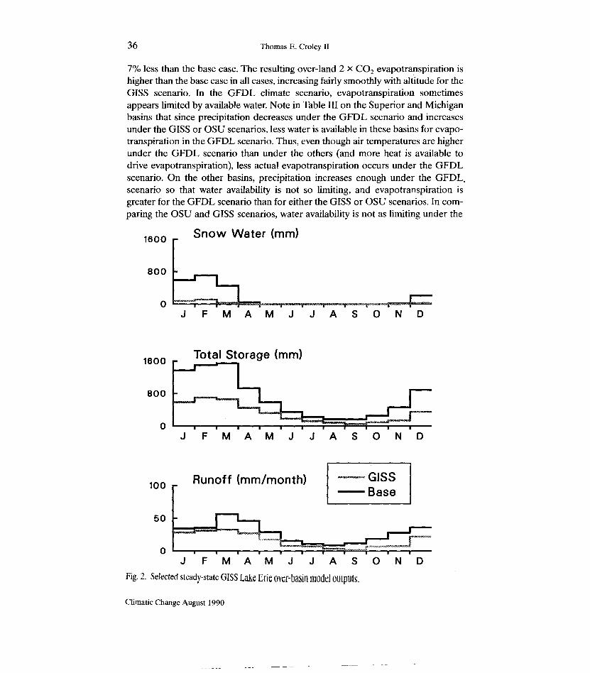
7% less than the base case. The resulting over-land 2 X CO, evapotranspiration is higher than the base case in all cases, increasing fairly smoothly with altitude for the GISS scenario. In the GFDL climate scenario, evapotranspiration sometimes appears limited by available water. Note in Table I11 on the Superior and Michigan basins that since precipitation decreases under the GFDL scenario and increases under the GISS or OSU scenarios, less water is available in these basins for evapotranspiration in the GFDL scenario. Thus, even though air temperatures are higher under the GFDL scenario than under the others (and more heat is available to drive evapotranspiration), less actual evapotranspiration occurs under the GFDL scenario. On the other basins, precipitation increases enough under the GFDL. scenario so that water availability is not so limiting, and evapotranspiration is greater for the GFDL scenario than for either the GISS or OSU scenarios. In comparing the OSU and GISS scenarios, water availability is not as limiting under the

1600 r Snow Water (mm)

800

0 J F M A M J J A S O N D

J F M A M J J A S O N D

100 Runoff (mmlmonth)

50

0 J F M A M J J A S O N D

Fig. 2. Selected steady-state GISS Lake Erie over-basin model outputs.



GISS scenario for the Superior and Michigan basins and more evapotranspiration occurs. For the other basins, GISS water availability is more limiting and less evapotranspiration occurs under the GISS scenario than under the OSU scenario even though the potential is greater (temperatures are higher).

On the Superior basin, the average steady-state snowpack storage is reduced more than 50% by higher air temperatures during the winter; on the other basins, more to the south, the snowpack is almost entirely absent under the GISS 2 x CO, scenario; see Table IV and the Erie example in Figure 2. The snow season (period of freezing air temperatures) is shortened also two weeks to one month under the GISS scenario. The reduced snowpack causes smaller derived moisture storages in the soil zone, groundwater, and surface zones; in some cases the total is reduced more than 50% in Figure 2 and Table IV Consequently, annual runoff is reduced in all cases, changing smoothly for the GISS scenario with longitude (see Table 111). Runoff peaks slightly earlier and with smaller magnitude under the 2 X CO, climate than under the base case, as reflected by total moisture storage for Lake Erie in Figure 2.

3.3. Lake Heat Balance

The over-lake air temperature, humidity, and wind speed differ from over-land since the lower atmospheric layer is affected by the water surface over which it lies. In general, for all 2 x CO, scenarios, the synergistic relationship that exists between over-lake air and water temperatures yields a general increase in both that follows the base case patterns, similar to over-land behavior. Table V shows that the average steady-state GISS annual over-lake air temperatures are 4.9-5.5 "C higher. An increase with latitude is more pronounced than variation with size of the lake in terms of volume or heat capacity although Lake Superior not only has the largest rise in over-lake air temperatures but also has the largest rise relative to over-land air temperature rise, probably reflecting the large heat storage capacity influence on the air layer over the lake. Absolute humidities over the lakes are higher for the 2 X CO, climate while cloud cover and over-water wind speed have dropped after adjustment of over-land values for over-water conditions at increased water temperatures.

The heat budget gives rise to increased water surface temperatures as seen for Lake Erie in Figure 3. Since Lake Erie is a very shallow lake with little heat storage, the annual cycle of the 2 X CO, water surface temperatures follows a pattern very similar to the base case but several degrees higher. The average steady-state GISS water surface temperatures in Table VI are 4.3-5.6 "C higher, reflecting again the general influence of heat storage capacty in a lake. Another influence not seen in Table VI is that the higher heat content of Lake Superior earlier in the year allows the 2 x CO, water surface temperatures to peak earlier than the base case; as over- lake Superior air temperatures are affected by the water temperatures, they also peak ahead of the base case.



evaporation may be large even with offsetting humidity and wind speed changes as evident in Tables V and VI. At lower air-water temperatures, the effects of humidity and wind speed changes become primary in determining the relative magnitudes of evaporation between the various scenarios.

The higher water surface temperatures under the 2 X CO, climate result in increased annual lake evaporation in Table VI. The shallow lakes have the largest .

absolute increase in evaporation under all 2 x CO, scenarios. Lake Michigan evaporation may be suspect because no data were used in the calibration of the Lake Michigan heat balance. Note that while average humidities are up and average wind speeds are down in Table IV (by themselves suggesting that evaporation drops), evaporation in Table VI is higher. This is because the water surface temperature (and associated saturated vapor pressure at the surface) has increased sufficiently. Interestingly, Lake Superior evaporation under the GISS scenario is less than that under the OSU scenario even though GISS water surface temperatures rise more than OSU. However, inspection shows that the GISS air temperature increase gives rise to a lower over-land-air-water temperature difference (see Tables I11 and VI) than the OSU scenario. Thus, air over Lake Superior is generally more stable under the GISS scenario than under the OSU scenario, resulting in larger corrections in air temperature and dewpoint toward the water surface temperature. Resulting air- water vapor pressure differences and wind speeds are lower (the latter is reflected in Table V) with consequent lower evaporation.

3.4. Net Basin Supply Components

Over-lake precipitation, runoff, and lake evaporation sum algebraically as the net basin supply and are presented again in Table VII for convenience. Since over-lake precipitation is taken here as the same as over-land, Table VII shows the same rela- tions for precipitation as does Table I11 but expressed as absolute differences. Runoff is also the same except it is expressed as a depth and absolute differences over the lake surface in Table VII instead of as depth over the basin surface and relative differences in Table 111. Net basin supply in the GISS scenario in Table VII is seen to be less under the 2 x CO, climate than under the base case; this is true throughout the year for Lakes St. Clair and Erie (see Figure 3 for Erie). It is nearly true on Lakes Huron (only January supplies are higher) and Ontario (only January and February are higher); Lake Michigan experiences increased net basin supplies during the winter under the GISS 2 x CO, scenario and Lake Superior has increased net basin supplies during the fall and winter. These drops in supplies are reflected in the annual GISS totals in Table VII. The GISS scenario results in a larger precipitation rise and a smaller drop in basin runoff for Lake Superior than do either the GFDL or OSU scenarios, resulting in a higher net basin supply and lower drop from the base case. The GISS scenario on Lake Michigan shows a larger precipitation rise and a smaller drop in basin runoff than the GFDL scenario. On the other lakes, the GISS scenario results in decreases in over-lake precipita-



TABLE VII: Average annual steady-state net supply components differences

Basin 1 X CO, over-lake precipitationa and 1 X CO, basin runoff a and 2 X CO, absolute differences 2 X CO, absolute differences


Superior 810mm 148mm -36mm 5 8 m m 6091nm - l l m m -159mm -<8mm Michigan 813 mm 16 mm -8 mm 42 mm 623 mm -152 mm -168 mm -87 mm Huron 855 mm -43 mm 28 mm 46 mm 823 mm -241 mm -158 mm -78 mm St. Clair 828 mm -53 mm 56 mm 51 mm 4379 mm -1870 mm -901 mm -891 mm Erie 893 mm -53 mm 48 mm 54 mm 796 mm -328 mm -173 mm -153 mm Ontario 923 mm -66 mm 27 rnrn 74 mm 1698 mm -565 mm -31 1 mm -1 12 rnrn

Basin 1 X CO, over-lake evaporation" and 1 X CO, net basin supply" and 2 x CO, absolute differences 2 x CO, relative changes


Superior 572 mm 152 mm 284 mm 173 mm 847 mm -2% -57% -19% Michigan 738 mm 176 mm 279 mm 179 mm 698 rnrn -45% -65% -32% Huron 627 mm 199 mm 297 mm 166 mm 1052 mm -46% -41% -19% St. Clair 813 mm 297 mm 408 mm 262 mm 4395 mm -50% -28% -25% Erie 1097 mm 290 mm 414 mm 232 mm 592 mm -1 13% -91% -56% Ontario 681 mm 213 rnm 281 mm 172 mm 1941 mm -43% -29% -1 1%

a Expressed as depths over the lake.

TABLE VIII: Average annual steady-state Great Lakes basin hydrology and net basin supply components

Scenario Over-land Evapotrans- Basin runoff Over-lake Over-lake Net basin precipitation piration (cm) (cm) precipitation evaporation supply (cm) (cm) ( 4 ( 4

BASE 13637 7727 6090 6499 5352 7237 '

GISS 13871 +2% 9317 21% 4658 -24% 6747 +4% 6821 +27% 4584 -37% GFDL 13725 +lO/o 9176 19% 4714 -23% 6501 +OO/o 7685 +44% 3530 -51% OSU 14483 +6% 9204 19% 5438 -11% 6903 +6% 6745 +26% 5596 -23%

tion (instead of increases as with the GFDL and OSU scenarios) and larger decreases in basin runoff and net basin supplies.

Table VIII and Figure 3 summarize the changes in the hydrologic and net basin supply components for the entire Great Lakes basin; they were computed by con- verting the equivalent depths of Table VII to annual flow rates on each lake and adding them over all the lakes. The changes from the, base case are also expressed relatively in Table VIII. Net basin supplies to all Great Lakes are seen to drop between about one quarter to one half under the various 2 x CO, scenarios. Even though more heat is available under the GFDL scenario than under the GISS or



OSU scenarios, evapotranspiration is lower because less water is available, as seen by inspection of the average precipitation. In the OSU and GISS scenarios, water availability is not as limiting and the higher air temperatures of the GISS scenario lead to higher evapotranspiration than in the OSU scenario even though more water is available under the OSU scenario.

3.5. Sensitivities

Although the GISS, GFDL, and OSU steady-state scenarios show conflicting estimates of precipitation change, each shows increases in air temperatures that significantly reduce the snowpack, especially in the southern basins. Thus, even if precipitation increases more than suggested by the GCMs, the snowpack still will be much reduced under warmer winters. Similarly, soil moisture storage and runoff peak shortly after snowmelt and then drop throughout the summer and fall due to high evapotranspiration; each climate scenario produces earlier snowmelt and a longer period of evapotranspiration. Although soil moisture and runoff certainly vary with precipitation, they are most sensitive to it in midsummer when at their annual mini- mums. Thus, within the limits of precipitation produced by the GCMs, soil moisture and runoff scenarios are relatively insensitive to precipitation.

As small air temperature rises, the rise in water surface temperature and the vapor pressure difference with the atmosphere compensate for the smaller drop in wind speed and rise in atmospheric humidity, and evaporation increases. For large air temperature rises, over-water stability increases, they do not compensate, and evaporation may decrease. This turn-around point occurs in the range of the three climate-change scenarios considered here, giving uncertainty in the evaporation estimates. Note also that increased over-water stability would alter over-lake precipitation but this is ignored in the GCMs (because of their large scale, the lakes do not appear) and therefore, is not considered here.

4. Transient-State Hydrologic Impacts

4.1. Methodology

We simulated one transient GISS scenario (Hansen et al., 1988) supplied by EPA representing the transition from the present climate to near the 2 X CO, climate during the period 1981-2060. Our general procedure was to first simulate 80 years of 'present' hydrologic component processes over the period 1981-2060. We did this by using historical daily maximum and minimum air temperatures, precipitation, wind speed, humidity, and cloud cover data for the 1951-80 period, repeated three times, and applied to initial conditions (basin moisture storages, lake heat storages, and water surface temperatures) observed 1 January, 1981; only the 80 years from 1 January, 1981 through 31 December, 2060 are of interest. We repeated the procedure developed for steady-state climate change investigations



three times (reported above). The first simulation used initial conditions observed 1 January, 1981; the second used the end-of-run conditions from the first simulation as initial conditions and the third used end-of-run conditions from the second. The three simulations were combined to represent the entire period of interest. After this 'base case' scenario was completed, we conducted simulations with adjusted data sets.

The EPA-supplied GISS transient scenario consisted of 9 sets of 12 monthly ratios for precipitation, air temperature, humidity, and cloud cover, and 12 monthly differences for wind speed, 1 set for each decade from 1970-9 through 2050-9. These ratios or differences were between 'present' and 'future' values for each of the data and represent atmospheric model predictions for an increasing atmospheric CO, content over the period 1971-2059. We used these ratios or differences by interpolating between decadal averages to obtain adjustments for each month of each year for the period 1981-2059 and by applying them in three simulations as for the base case: 1981-2010 adjustments to 1951-80 data for the 1981-2010 period simulation, 2011-40 adjustments to 1951-80 data for the 2011-40 simulation, and 2041-59 adjustments to 1951-1969 data for the 2041- 59 simulation. We took the 2060 adjustment as the same as the 2059 adjustment, since the GISS scenario ended in 2059, and applied it to 1970 data for the 2060 simulation. Discerning the 2 x CO, signal from the historical variations in the adjusted data sets is enhanced by comparing values 30 years apart, thus eliminating the (repetitive) historical variations. A differencing approach that does this is described following. We combined ratios for each month of each year of the simulation from the nearest atmospheric model grid point for each and every square kilometer representing a watershed or a lake surface to derive areally-averaged adjustments to apply to our areally-averaged data sets for each watershed or lake surface. We then used the transient scenario segments in simulations, as we did with the original historical data, combining them to represent the entire period of interest and then interpreted differences between the transient scenario and the base case scenario as resulting from the changing climate.

There are serious difficulties in analyzing transient impacts of climate change with short historical data sets. In simulating 80 years (1981-2060) by using 30 years of historical data (1951-80) repeated three times (for the 1981-2010,2011- 2040, and 2041-2060 periods), the variations contained in the historical record repeat. As corrections to the historical data are made to reflect the transient GISS climate changes, it is found that the repeating fluctuations of the historical record so completely dominate the superimposed climate changes that it is difficult to see the effect of climate change. Thirty-year averages could be used to filter historical variations for presentation of results; however, only two complete 30-yr periods are contained in the simulation and a 30-yr average filters some of the climatic change as well. A differencing approach is used here to give a very general idea of transient behavior and it works by comparing transient behavior 30 years apart to eliminate the effect of the historical variations. By comparing the GISS and base cases tran-



sient simulation changes for decades 1,4, and 7 (1981-90,2011-20, and 2041-50 which are all based on the same 1951-60 data period), decades 2,5, and 8 (1991- 00,2021-30, and 2051-60 which are all based on the same 1961-70 data period), and decades 3 and 6 (2001-10 and 2031-40 which are both based on the same 1971-80 data period), the effect of the repetitive natural variations is eliminated since the same underlying historical data segments are used in each grouping; this is illustrated in detail in the following section for air temperatures. The climate change trends then can be identified.

4.2. Hydrological Changes

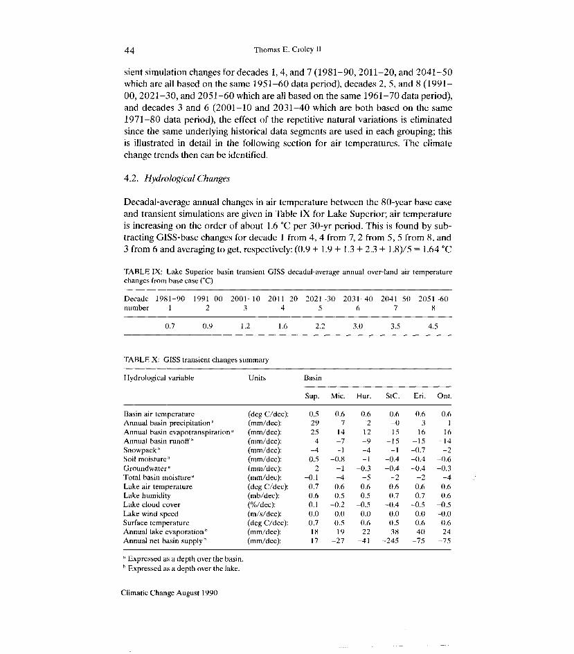
Decadal-average annual changes in air temperature between the 80-year base case and transient simulations are given in Table IX for Lake Superior; air temperature is increasing on the order of about 1.6 "C per 30-yr period. This is found by sub- tracting GISS-base changes for decade 1 from 4 , 4 from 7,2 from 5 , 5 from 8, and 3 from 6 and averaging to get, respectively: (0.9 + 1.9 + 1.3 + 2.3 + 1.8)/5 = 1.64 "C

TABLE IX: Lake Superior basin transient GISS decadal-average annual over-land air temperature changes from base case ("C)

Decade 1981-90 1991-00 2001-10 201 1-20 2021-30 2031-40 2041-50 2051-60 number 1 2 3 4 5 6 7 8

TABLE X: GISS transient changes summary

Hydrological variable Units Basin

Sup. Mic. Hur. StC. Eri. Ont.

Basin air temperature Annual basin precipitationu Annual basin evapotranspiration Annual basin runoff" Snowpack " Soil moisture" Groundwater" Total basin moisture" Lake air temperature Lake humidity Lake cloud cover Lake wind speed Surface temperature Annual lake evaporation Annual net basin supply

(deg C/dec): (mm/dec):

" (mm/dec): (mm/dec): (mm/dec): (mrn/dec): (mm/dec): (mm/dec): (deg C/dec): (mb/dec): (%/dec): (m/s/dec): (deg C/dec): (mm/dec): (mm/dec):

;' Expressed as a depth over the basin. Expressed as a depth over the lake.



per 30 years. This is more conveniently expressed as 0.5 "C per decade. Other hydrometeorological quantity variations are computed in the same way and are summarized in Table X.

On Lake Superior, precipitation increases are partially offset by evapotranspira-. tion increases so that annual runoff, expressed as a depth over the land portion of the basin, increases about 4 mm each decade. All other lakes show a drop in annual runoff of 7-15 mm/decade. The average snowpack accumulates about 1-4 mrn less each decade and average soil zone moisture and groundwater generally drop 0.3-1 mm/decade (except on Superior); the resultant effect is a lowering of total basin moisture storage about 0.1-5 mm/decade. Over-lake air temperatures increase at about the same rate as over-land air temperatures. Over-lake humidity generally increases slightly (but negligibly) each decade; note however that while it is corrected for over-water conditions in the simulations, it is not computed by taking increased evaporation into account. Rather, over-land humidity was supplied in the GISS atmospheric model outputs (inputs to this simulation). Cloud cover generally decreases slightly (but negligibly) and is not influenced by these simulations; it is strictly an input here from the GISS atmospheric model. Over-lake wind speed is almost not affected and the water surface temperature increases by about 0.5-0.7 "C each decade. Resultant annual lake evaporation increases 18-40 mm/decade. Net basin supplies are highly variable but generally drop on all lakes except Superior.

5. Summary

The study results should be received with caution as they are of course dependent on the GCM outputs with large uncertainties. Furthermore, changes in variabilities that would take place under a changed climate are not addressed. Seasonal timing differences under a changed climate are not reproduced from the GCMs with the method of coupling used herein and seasonal meteorology patterns are preserved as they exist in the historical data. Seasonal changes induced by the changed meteorology because of a time-lag storage effect are observable however. Shifts in snowpack or water surface temperature growth and decay are examples. Changes in annual variability are less clear, again as a result of using the same historical time structure for both the base case and the changed climate scenarios.

The higher air temperatures under the steady-state 2 X CO, scenarios lead to higher over-land evapotranspiration and lower runoff to the lakes with earlier runoff peaks since the snowpack is reduced up to 10O0/0 and the snow season is shortened from two to four weeks. This also results in more than a 50% reduction in available soil moisture. Under the warmer scenarios on some lakes, water availability limits evapotranspiration so that more occurs under wetter (and cooler) scenarios.

Water surface temperatures peak earlier on Lake Superior; since the climate becomes similar to present-day climates on the southern lakes, the lake tempera-



ture behaves similar to present-day southern deep Great Lakes. There are larger amounts of heat resident in the deep lakes throughout the year. Also, buoyancy- driven turnovers of the water column, related to the passage of water temperatures through that at maximum density, occur only on the shallow lakes (St. Clair and Erie) and only rarely on Lake Superior under the OSU scenario; otherwise they do not occur at all. Currently, they occur twice a year on all lakes. The lakes still might experience a single winter turnover if temperature gradients are small and winds are strong enough to induce turbulent mixing. Ice formation is greatly reduced over winter on the deep Great Lakes and lake evaporation increases on all lakes.

The average steady-state net basin supplies to all lakes but St. Clair are seen to drop 16-844 mm/yr for the GISS 2 X CO, scenario, 427-564 mm/yr for the GFDL, and 163-331 mm/yr for the OSU scenario. Over the entire Great Lakes basin, the three scenarios result in a 23 to 51% reduction of net basin supplies and they vary in the magnitude of the components of those supplies (particularly basin runoff and lake evaporation). Analysis of a GISS 80-yr transient scenario indicates that while supplies to Lake Superior increase, the other lakes (except St. Clair) experience drops in annual net basin supplies at 27-75 rnrn/decade.

References

Bolsenga, S. J.: 1977, 'Lake-Land Precipitation Relationships Using Northern Lake Michigan Data', J. Appl. Met. 16 (Il), 1158-1164.

Bolsenga, S. J.: 1979, 'Determining Overwater Precipitation from Overland Data: The Methodological Controversy Analyzed; J. Great Lakes Res. 5 (3-4), 301-311.

Bolsenga, S. J. and Hagman, J. C.: 1975, 'On the Selection of Representative Stations for Thiessen Polygon Networks to Estimate Lake Ontario Overwater Precipitation', International Field Year for the Great Lakes Bulletin 16, National Oceanic and Atmospheric Administration, Rockville, Mary- land, pp. 57-62.

Cohen, S. J.: 1986, 'Impacts of C0,-Induced Climatic Change on Water Resources in the Great L,akes Basin', Climatic Change 8, 135-153.

Cohen, S. J.: 1987, 'Sensitivity of Water Resources in the Great Lakes Region to Changes in Tempera- ture, Precipitation, Humidity, and Wind Speed', Proceedings of the Symposium, The Influence of Climate Change and Climatic kriability on the Hydrologic Regime and Water Resources, IAHS Publ. no. 168, Vancouver, August 1987, pp. 489-499.

Croley, T. E., 11: 1982, 'Great Lakes Basins Runoff Modeling', NOAA Tech. Memo. ERL GLERL-39, Natl. Tech. Inf. Ser., Springfield, Va. 22161.

Croley, T. E., 11: 1983a, 'Great Lakes Basins (U.S.A.-Canada) Runoff Modeling', J. Hydrol. 64, 135- 158.

Croley, T. E., 11: 1983b, 'Lake Ontario Basin (USA.-Canada) Runoff Modeling', J. Hydrol. 66, 101- 121.

Croley, T. E., 11: 1989, 'Verifiable Evaporation Modeling on the Laurentian Great Lakes', Wat. Resour. Res. 25 (5), 781-792.

Croley, T. E., I1 and Hartmann, H. C.: 1984, 'Lake Superior Basin Runoff Modeling', NOAA Tech. Memo. ERL GLERL-50, Natl. Tech. Inf. Ser., Springfield, Va. 22161.

Croley, T. E., I1 and Hartmann, H. C.: 1985a, 'Lake Champlain Water Supply Forecasting', GLERL Open File Report, Contribution No. 450, Great Lakes Environmental Research Laboratory, Ann Arbor, Michigan.

Croley, T. E., I1 and Hartmann, H. C.: 1985b, 'Resolving Thiessen Polygons', J. Hydrol. 76,363-379. Croley, T. E., I1 and Hartmann, H. C.: 1986, 'Near-Real-Time Forecasting of Large-Lake Water Sup-


Laurentian Great Lakes Double-COz 47

plies; A User's Manual: NOAA Tech. Memo. ERL GLERL-61, Environmental Research Laborato- ries, Boulder, Colorado.

Croley, T. E., I1 and Hartman, H. C.: 1987, 'Near Real-Time Forecasting of Large Lake Supplies', J. Wat. Res. Plan. Manag. Div. 113 (6), 810-823.

Ghan, S. J. et al.: 1982, 'A Documentation of the OSU Two-Level Atmospheric GCM', CRI Report 35, Oregon State Univ.

Hansen, J., Fung, I., Lacis, A., Rind, D., Lebedeff, S., Ruedy, R., Russel, G., and Stone, P.: 1988, 'Global Climate Changes as Forecast by Goddard Institute for Space Studies Three-Dimensional Model', J. G. Res. 93,9341-9364.

Hansen, J., Russell, G., Rind, D., Stone, P., Lacis, A., Lebedeff, S., Ruedy, R., and Travis, L.: 1983, 'Efficient Three-Dimensional Global Models for Climate Studies: Models I and II', Monthly Weather Review 111 (4), 609-662.

Hutchinson, G. E.: 1957, A Treatise on Limnology, Volume I, Part 1 - Geography and Physics of Lakes, John Wiley and Sons, New York, New York.

Manabe, S. and Wetherald, R. T.: 1987, 'Large-Scale Changes in Soil Wetness Induced by an Increase in Carbon Dioxide', J. Atmos. Sci. 44, 1211-1235.

Quinn, E H. and Croley, T. E., IL: 1983, 'Climatic Water Balance Models for Great Lakes Forecasting and Simulation', in Preprint Volume: Fifh Conference on Hydrometeorology, American Meteorologi- cal Society, Boston, Massachusetts, pp. 218-223.

U.S. Environmental Protection Agency: 1984, Potential Climatic Impacts of Increasing Atmospheric CO, with Emphasis on Water Availability and Hydralogy in the United States, EPA Office of Policy, Planning, and Evaluation, Washington, D.C.

U.S. Environmental Protection Agency: 1988, The Potential Effects of Global Climate Change on the United States. Draf Report to Congress, J . B. Smith and D. A. Tirpak, Eds., EPA Office of Policy, Planning, and Evaluation, Washington, D.C.

Wilson, J. W.: 1977, 'Effect of Lake Ontario on Precipitation: Monthly Weather Review 105,207-214.

(Received 6 December, 1988; in revised form 19 October, 1989)


Documents

LAURENTIAN GREAT LAKES DOUBLE-CO, CLIMATE … · LAURENTIAN GREAT LAKES DOUBLE-CO, CLIMATE CHANGE HYDROLOGICAL IMPACTS ' ... supplies during the late fall and winter months I' when