Embed Size (px)
Citation preview
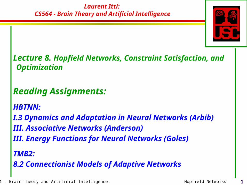
1Laurent Itti: CS564 - Brain Theory and Artificial Intelligence. Hopfield Networks
Laurent Itti: CS564 - Brain Theory and Artificial Intelligence
Lecture 8. Hopfield Networks, Constraint Satisfaction, and Optimization
Reading Assignments:
HBTNN:
I.3 Dynamics and Adaptation in Neural Networks (Arbib)
III. Associative Networks (Anderson)
III. Energy Functions for Neural Networks (Goles)
TMB2:
8.2 Connectionist Models of Adaptive Networks
2Laurent Itti: CS564 - Brain Theory and Artificial Intelligence. Hopfield Networks
Hopfield Networks
A paper by John Hopfield in 1982 was the catalyst in attracting the attention of many physicists to "Neural Networks".
In a network of McCulloch-Pitts neurons
whose output is 1 iff wij sj i and is otherwise 0,
neurons are updated synchronously: every neuron processes its inputs at each time step to determine a new output.
3Laurent Itti: CS564 - Brain Theory and Artificial Intelligence. Hopfield Networks
Hopfield Networks
A Hopfield net (Hopfield 1982) is a net of such units subject to the asynchronous rule for updating one neuron at a time:
"Pick a unit i at random.
If wij sj i, turn it on.
Otherwise turn it off."
Moreover, Hopfield assumes symmetric weights:
wij = wji
4Laurent Itti: CS564 - Brain Theory and Artificial Intelligence. Hopfield Networks
“Energy” of a Neural Network
Hopfield defined the “energy”:
E = - ½ ij sisjwij + i sii
If we pick unit i and the firing rule (previous slide) does not change its si, it will not change E.
5Laurent Itti: CS564 - Brain Theory and Artificial Intelligence. Hopfield Networks
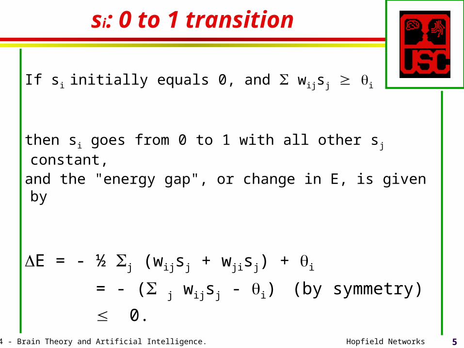
si: 0 to 1 transition
If si initially equals 0, and wijsj i
then si goes from 0 to 1 with all other sj constant,
and the "energy gap", or change in E, is given by
E = - ½ j (wijsj + wjisj) + i
= - ( j wijsj - i) (by symmetry)
0.
6Laurent Itti: CS564 - Brain Theory and Artificial Intelligence. Hopfield Networks
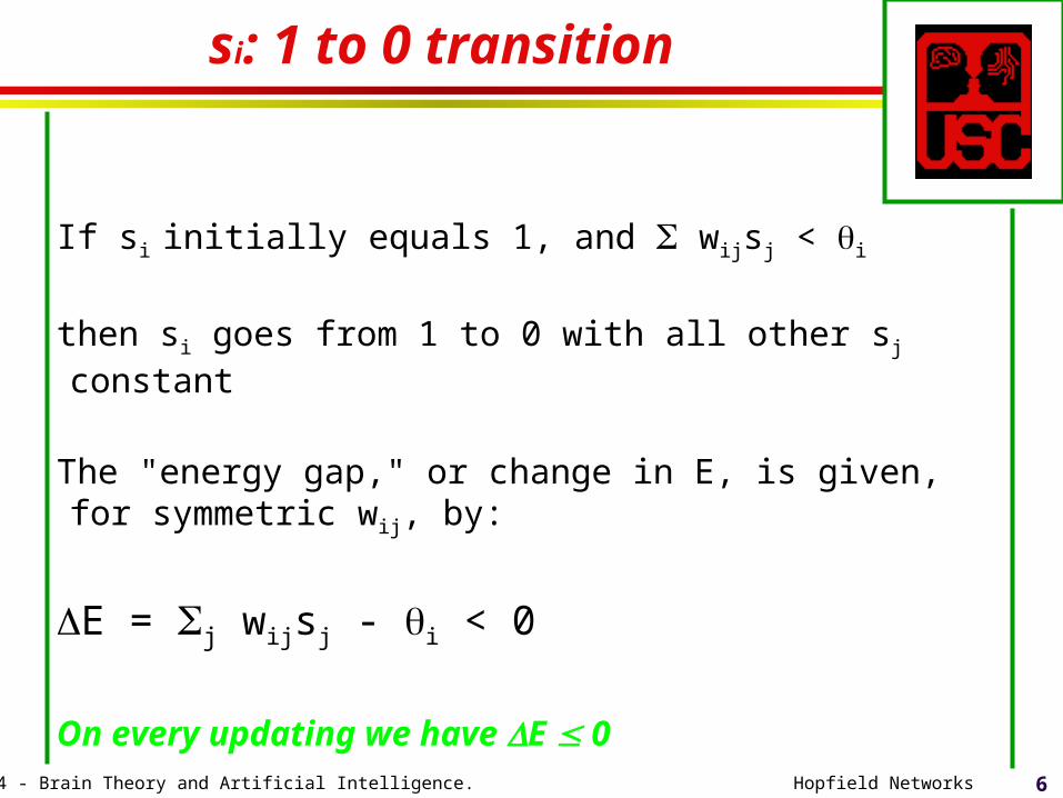
si: 1 to 0 transition
If si initially equals 1, and wijsj < i
then si goes from 1 to 0 with all other sj constant
The "energy gap," or change in E, is given, for symmetric wij, by:
E = j wijsj - i < 0
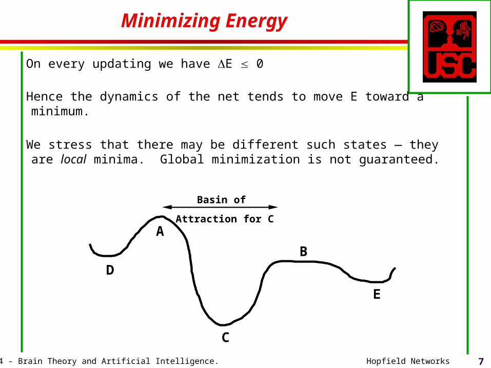
On every updating we have E 0
7Laurent Itti: CS564 - Brain Theory and Artificial Intelligence. Hopfield Networks
Minimizing Energy
On every updating we have E 0
Hence the dynamics of the net tends to move E toward a minimum.
We stress that there may be different such states — they are local minima. Global minimization is not guaranteed.
B
C
A
Basin of
Attraction for C
D
E
8Laurent Itti: CS564 - Brain Theory and Artificial Intelligence. Hopfield Networks
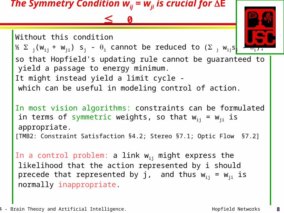
The Symmetry Condition wij = wji is crucial for E 0
Without this condition ½ j(wij + wji) sj - i cannot be reduced to ( j wijsj - i),
so that Hopfield's updating rule cannot be guaranteed to yield a passage to energy minimum.
It might instead yield a limit cycle - which can be useful in modeling control of action.
In most vision algorithms: constraints can be formulated in terms of symmetric weights, so that wij = wji is appropriate.
[TMB2: Constraint Satisfaction §4.2; Stereo §7.1; Optic Flow §7.2]
In a control problem: a link wij might express the likelihood that the action represented by i should precede that represented by j, and thus wij = wji is normally inappropriate.
9Laurent Itti: CS564 - Brain Theory and Artificial Intelligence. Hopfield Networks
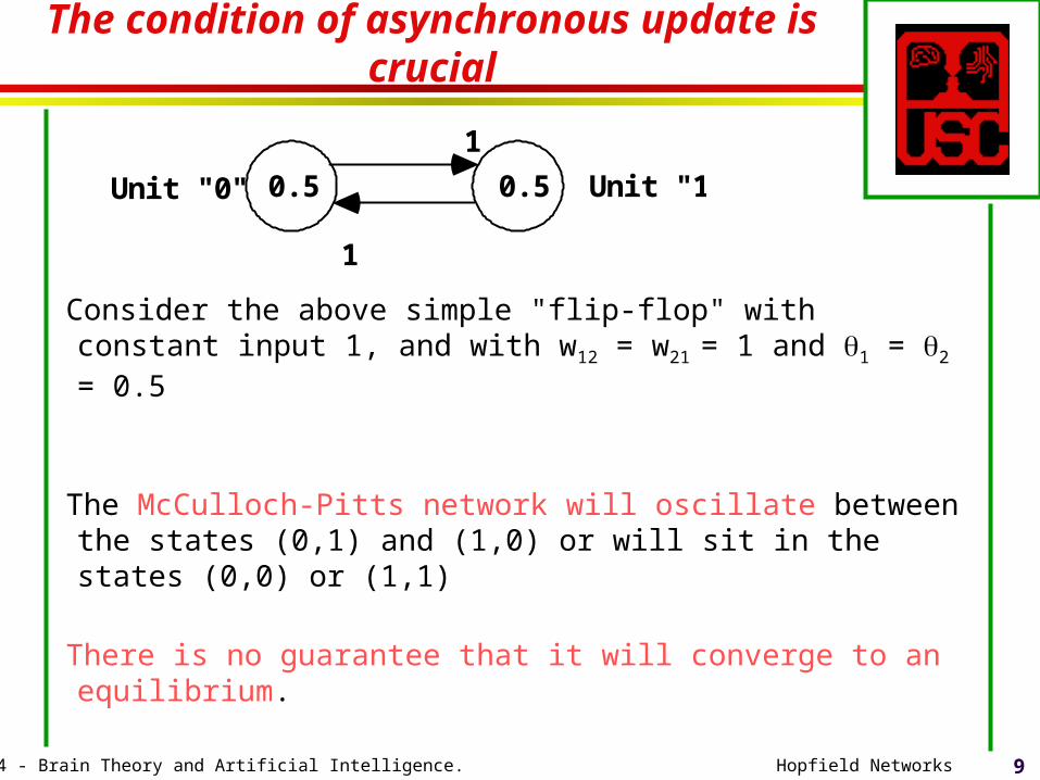
The condition of asynchronous update is crucial
Consider the above simple "flip-flop" with constant input 1, and with w12 = w21 = 1 and 1 = 2 = 0.5
The McCulloch-Pitts network will oscillate between the states (0,1) and (1,0) or will sit in the states (0,0) or (1,1)
There is no guarantee that it will converge to an equilibrium.
1
1
0.50.5Unit "0" Unit "1"
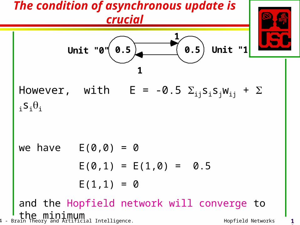
10Laurent Itti: CS564 - Brain Theory and Artificial Intelligence. Hopfield Networks
The condition of asynchronous update is crucial
1
1
0.50.5Unit "0" Unit "1"
However, with E = -0.5 ijsisjwij + isii
we have E(0,0) = 0
E(0,1) = E(1,0) = 0.5
E(1,1) = 0
and the Hopfield network will converge to the minimum
at (0,0) or (1,1).
11Laurent Itti: CS564 - Brain Theory and Artificial Intelligence. Hopfield Networks
Hopfield Nets and Optimization
To design Hopfield nets to solve optimization problems: given a problem, choose weights for the network so that E is a measure of the overall constraint violation.
A famous example is the traveling salesman problem.[HBTNN articles:Neural Optimization; Constrained Optimization and the Elastic Net. See also TMB2 Section 8.2.]
Hopfield and Tank 1986 have constructed VLSI chips for such networks which do indeed settle incredibly quickly to a local minimum of E.
Unfortunately, there is no guarantee that this minimum is an optimal solution to the traveling salesman problem. Experience shows it will be "a pretty good approximation," but conventional algorithms exist which yield better performance.
12Laurent Itti: CS564 - Brain Theory and Artificial Intelligence. Hopfield Networks
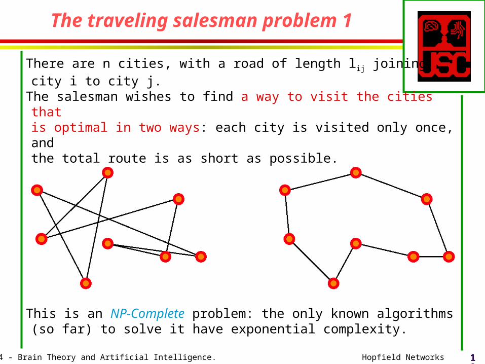
The traveling salesman problem 1
There are n cities, with a road of length lij joining city i to city j.
The salesman wishes to find a way to visit the cities that is optimal in two ways: each city is visited only once,
and the total route is as short as possible.
This is an NP-Complete problem: the only known algorithms (so far) to solve it have exponential complexity.
13Laurent Itti: CS564 - Brain Theory and Artificial Intelligence. Hopfield Networks
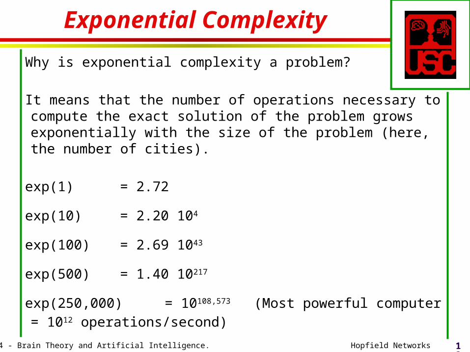
Exponential Complexity
Why is exponential complexity a problem?
It means that the number of operations necessary to compute the exact solution of the problem grows exponentially with the size of the problem (here, the number of cities).
exp(1) = 2.72
exp(10) = 2.20 104
exp(100) = 2.69 1043
exp(500) = 1.40 10217
exp(250,000) = 10108,573 (Most powerful computer = 1012 operations/second)
14Laurent Itti: CS564 - Brain Theory and Artificial Intelligence. Hopfield Networks
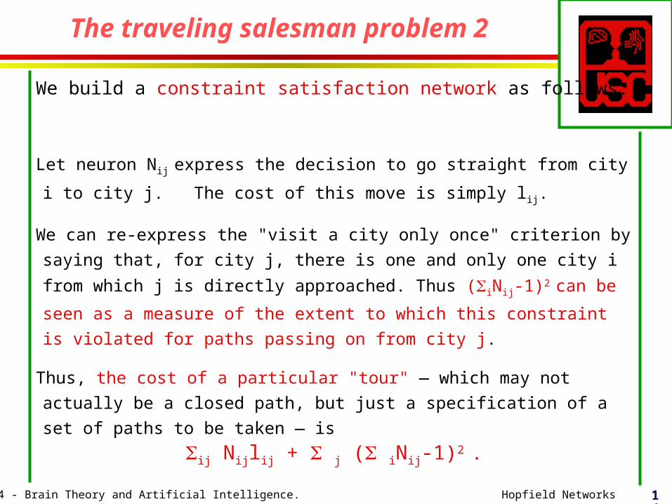
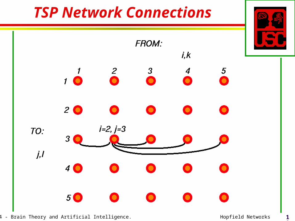
The traveling salesman problem 2
We build a constraint satisfaction network as follows:
Let neuron Nij express the decision to go straight from city i to
city j. The cost of this move is simply lij.
We can re-express the "visit a city only once" criterion by
saying that, for city j, there is one and only one city i from
which j is directly approached. Thus (iNij-1)2 can be seen as a
measure of the extent to which this constraint is violated for
paths passing on from city j.
Thus, the cost of a particular "tour" — which may not actually
be a closed path, but just a specification of a set of paths to
be taken — is
ij Nijlij + j ( iNij-1)2 .
15Laurent Itti: CS564 - Brain Theory and Artificial Intelligence. Hopfield Networks
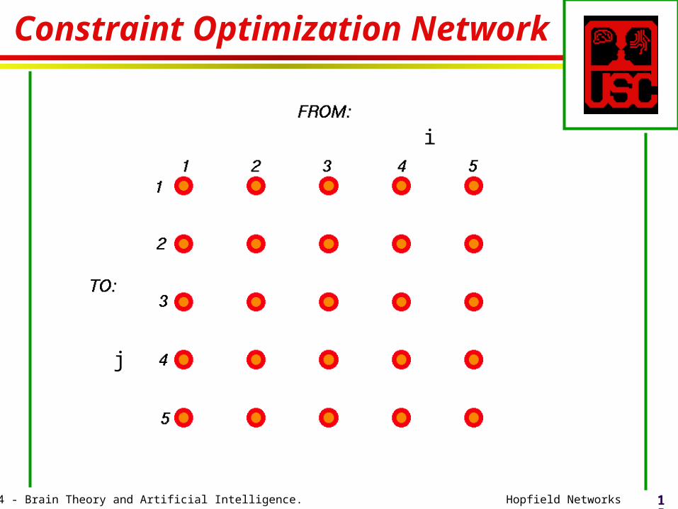
Constraint Optimization Network
i
j
16Laurent Itti: CS564 - Brain Theory and Artificial Intelligence. Hopfield Networks
The traveling salesman problem 3
Cost to minimize: ij Nijlij + j ( iNij-1)2
Now ( iNij-1)2 = ikNijNkj - 2 iNij + 1
and so j( iNij-1)2 = ijkNijNkj - 2 ijNij + n
= ij,kl NijNklvij,kl - 2 ijNij + n
where n is the number of citiesvij,kl equals 1 if j = l, and 0 otherwise.
Thus, minimizing ij Nijlij + j ( iNij-1)2 is equiv to minimizing
ij,kl NijNklvij,kl + ijNij(lij-2)
since the constant n makes no difference.
17Laurent Itti: CS564 - Brain Theory and Artificial Intelligence. Hopfield Networks
The traveling salesman problem 4
minimize: ij,kl NijNklvij,kl + ijNij(lij-2)
Compare this to the general energy expression (with si now replaced by Nij):
E = -1/2 ij,kl NijNklwij,kl + ij Nijij.
Thus if we set up a network with connections
wij,kl = -2 vij,kl ( = -2 if j=l, 0 otherwise) and ij = lij - 2, it will settle to a local minimum of E.
18Laurent Itti: CS564 - Brain Theory and Artificial Intelligence. Hopfield Networks
TSP Network Connections
19Laurent Itti: CS564 - Brain Theory and Artificial Intelligence. Hopfield Networks
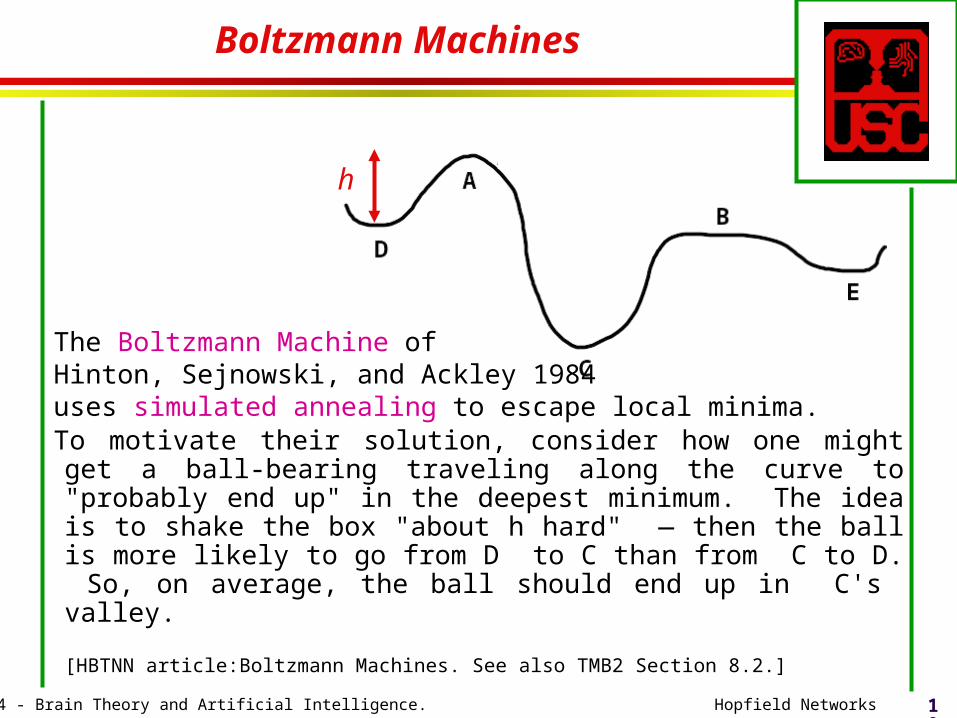
h
Boltzmann Machines
The Boltzmann Machine of Hinton, Sejnowski, and Ackley 1984uses simulated annealing to escape local minima.To motivate their solution, consider how one might get a ball-bearing traveling along the curve to "probably end up" in the deepest minimum. The idea is to shake the box "about h hard" — then the ball is more likely to go from D to C than from C to D. So, on average, the ball should end up in C's valley.
[HBTNN article:Boltzmann Machines. See also TMB2 Section 8.2.]
20Laurent Itti: CS564 - Brain Theory and Artificial Intelligence. Hopfield Networks
Boltzmann’s statistical theory of gases
In the statistical theory of gases, the gas is described not by a deterministic dynamics, but rather by the probability that it will be in different states.
The 19th century physicist Ludwig Boltzmann developed a theory that included a probability distribution of temperature (i.e., every small region of the gas had the same kinetic energy).
Hinton, Sejnowski and Ackley’s idea was that this distribution might also be used to describe neural interactions, where low temperature T is replaced by a small noise term T (the neural analog of random thermal motion of molecules).
21Laurent Itti: CS564 - Brain Theory and Artificial Intelligence. Hopfield Networks
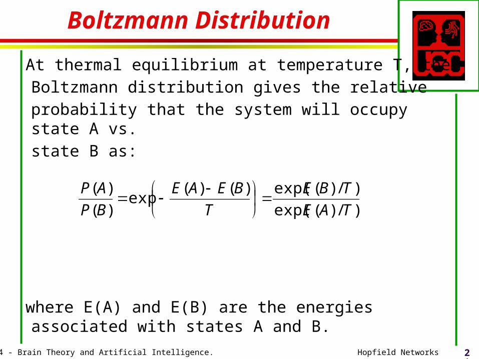
Boltzmann Distribution
At thermal equilibrium at temperature T, the Boltzmann distribution gives the relative probability that the system will occupy state A vs. state B as:
where E(A) and E(B) are the energies associated with states A and B.
)/)(exp(
)/)(exp()()(exp
)(
)(
TAE
TBE
T
BEAE
BP
AP
22Laurent Itti: CS564 - Brain Theory and Artificial Intelligence. Hopfield Networks
Simulated Annealing
Kirkpatrick et al. 1983: Simulated annealing is a general method for making likely the escape from local minima by allowing jumps to higher energy states.
The analogy here is with the process of annealing used by a craftsman in forging a sword from an alloy.
He heats the metal, then slowly cools it as he hammers the blade into shape. If he cools the blade too quickly the metal will form patches of different composition;
If the metal is cooled slowly while it is shaped, the constituent metals will form a uniform alloy.
[HBTNN article: Simulated Annealing.]
23Laurent Itti: CS564 - Brain Theory and Artificial Intelligence. Hopfield Networks
Simulated Annealing in Hopfield Nets
- Pick a unit i at random- Compute E = j wijsj - i that would result from flipping si
- Accept to flip si with probability 1/[1+exp(E/T)]
NOTE: this rule converges to the deterministic rule in the previous slides when T0
Optimization with simulated annealing:-set T-optimize for given T- lower T (see Geman & Geman, 1984)
-repeat
24Laurent Itti: CS564 - Brain Theory and Artificial Intelligence. Hopfield Networks
Statistical Mechanics of Neural Networks
A good textbook which includes research by physicists studying neural networks:
Hertz, J., Krogh. A., and Palmer, R.G., 1991, Introduction to the Theory of Neural Computation, Santa Fe Institute Studies in the Sciences of Complexity, Addison-Wesley.
The book is quite mathematical, but has much accessible material, exploiting the analogy between neuron state and atomic “spins” in a magnet.
[cf. HBTNN: Statistical Mechanics of Neural Networks (Engel and Zippelius)]


![Abstract arXiv:1607.05836v3 [cs.CV] 22 Jan 2017 · Improved Deep Learning of Object Category using Pose Information Jiaping Zhao, Laurent Itti University of Southern California fjiapingz,](https://img.pdfslide.us/doc/110x75/5e99b219c43ce4116369dd5a/abstract-arxiv160705836v3-cscv-22-jan-2017-improved-deep-learning-of-object.jpg)