Lattice reduction in two dimensions: analyses under

HAL Id: hal-00211495https://hal.archives-ouvertes.fr/hal-00211495

Preprint submitted on 21 Jan 2008

HAL is a multi-disciplinary open accessarchive for the deposit and dissemination of sci-entific research documents, whether they are pub-lished or not. The documents may come fromteaching and research institutions in France orabroad, or from public or private research centers.

L’archive ouverte pluridisciplinaire HAL, estdestinée au dépôt et à la diffusion de documentsscientifiques de niveau recherche, publiés ou non,émanant des établissements d’enseignement et derecherche français ou étrangers, des laboratoirespublics ou privés.

Lattice reduction in two dimensions : analyses underrealistic probabilistic models

Brigitte Vallée, Antonio Vera

To cite this version:Brigitte Vallée, Antonio Vera. Lattice reduction in two dimensions : analyses under realistic proba-bilistic models. 2008. hal-00211495

https://hal.archives-ouvertes.fr/hal-00211495

https://hal.archives-ouvertes.fr

Lattice reduction in two dimensions:analyses under realistic probabilistic models

Brigitte Vallee and Antonio Vera

CNRS UMR 6072, GREYC, Universite de Caen, F-14032 Caen, France

The Gaussian algorithm for lattice reduction in dimension 2 is precisely analysed under a class of realistic probabilisticmodels, which are of interest when applying the Gauss algorithm “inside” the LLL algorithm. The proofs deal withthe underlying dynamical systems and transfer operators. All the main parameters are studied: execution parameterswhich describe the behaviour of the algorithm itself as well as output parameters, which describe the geometry ofreduced bases.

Keywords: Lattice Reduction, Gauss’ algorithm, LLL algorithm, Euclid’s algorithm, probabilistic analysis of algo-rithms, Dynamical Systems, Dynamical analysis of Algorithms.

1 IntroductionThe lattice reduction problem consists in finding a short basis of a lattice of Euclidean space given aninitially skew basis. This reduction problem plays a primary role in many areas of computer scienceand computational mathematics: for instance, modern cryptanalysis [18], computer algebra [24], integerlinear programming [14], and number theory [7].

In the two-dimensional case, there exists an algorithm due to Lagrange and Gauss which computes inlinear time a minimal basis of a lattice. This algorithm is in a sense optimal, from both points of view ofthe time-complexity and the quality of the output. It can be viewed as a generalization of the EuclideanAlgorithm to the two dimensional-case. Forn≥ 3, the LLL algorithm [13] due to Lenstra, Lenstra andLovasz, computes a reduced basis of ann-dimensional lattice in polynomial time. However, the notion ofreduction is weaker than in the casen = 2, and the exact complexity of the algorithm (even in the worst-case, and for small dimensions) is not precisely known. The LLL algorithm uses as a main procedure theGauss Algorithm.This is why it is so important to have a precise understanding of the Gauss Algorithm. First, because thisis a central algorithm, but also because it plays a primary role inside the LLL algorithm. The geometryof then-dimensional case is involved, and it is easier to well understand the (hyperbolic) geometry of thecomplex plane which appears in a natural way when studying the Gauss Algorithm.

1365–8050c© 2003 Discrete Mathematics and Theoretical Computer Science (DMTCS), Nancy, France

2 B. Vallee and A. Vera

The previous results. Gauss’ algorithm has been analyzed in the worst case by Lagarias, [11], thenVallee [20], who also describes the worst-case input. Then, Daude, Flajolet and Vallee [8] completed thefirst work [9] and provided a detailed average-case analysis of the algorithm, in a natural probabilisticmodel which can be called a uniform model. They study the mean number of iterations, and prove thatit is asymptotic to a constant, and thus essentially independent of the length of the input. Moreover, theyshow that the number of iterations follows an asymptotic geometric law, and determine the ratio of thislaw. On the other side, Laville and Vallee [12] study the geometry of the outputs, and describe the law ofsome output parameters, when the input model is the previous uniform model.The previous analyses only deal with uniform-distributed inputs and it is not possible to apply these results“inside” the LLL algorithm, because the distribution of “local bases” which occur along the execution ofthe LLL algorithm is far from uniform. Akhavi, Marckert and Rouault [2] showed that, even in the uniformmodel where all the vectors of the input bases are independently and uniformly drawn in the unit ball, theskewness of “local bases” may vary a lot. It is then important to analyse the Gauss algorithm in a modelwhere the skewness of the input bases may vary. Furthermore, it is natural from the works of Akhavi [1]to deal with a probabilistic model where, with a high probability, the modulus of the determinant det(u,v)of a basis(u,v) is much smaller than the product of the lengths|u| · |v|. More precisely, a natural model isthe so–called model of valuationr, where

P[(u,v);

|det(u,v)|max(|u|, |v|)2 ≤ y

]= Θ(yr+1), with (r >−1).

Remark that, whenr tends to -1, this model tends to the “one dimensional model”, whereu andv arecolinear. In this case, the Gauss Algorithm “tends” to the Euclidean Algorithm, and it is important toprecisely describe this transition. This model “with valuation” was already presented in [21, 22] in aslightly different context, but not deeply studied.

Our results. In this paper, we perform an exhaustive study of the main parameters of Gauss algorithm,in this scale of distributions, and obtain the following results:

(i) We first relate the output density of the algorithm to a classical object of the theory of modularforms, namely the Eisenstein series, which are eigenfunctions of the hyperbolic Laplacian [Theorem 2].

(ii) We also focus on the properties of the output basis, and we study three main parameters: the firstminimum, the Hermite constant, and the orthogonal projection of a second minimum onto the orthogonalof the first one. They all play a fundamental role in a detailed analysis of the LLL algorithm. We relatetheir “contour lines” with classical curves of the hyperbolic complex plane [Theorem 3] and provide sharpestimates for the distribution of these output parameters [Theorem 4].

(iii ) We finally consider various parameters which describe the execution of the algorithm (in a moreprecise way than the number of iterations), namely the so–called additive costs, the bit-complexity, thelength decreases, and we analyze their probabilistic behaviour [Theorems 5 and 6].

Along the paper, we explain the role of the valuationr, and the transition phenomena between the GaussAlgorithm and the Euclidean algorithms which occur whenr →−1.

Towards an analysis of the LLL algorithm. The present work thus fits as a component of a moreglobal enterprise whose aim is to understand theoretically how the LLL algorithm performs in practice,and to quantify precisely the probabilistic behaviour of lattice reduction in higher dimensions.

Lattice reduction in two dimensions: analyses under realistic probabilistic models 3

Figure 1: On the left: experimental results for the ratio(1/n) log |b1|(detL)1/n [here,n is the dimension,b1 is the first

vector of the LLL reduced basis and detL is the determinant of the latticeL]. On the right, the output distribution of“local bases” for the LLL algorithm (see Sections 3.8 and 4.7).

We are particularly interested in understanding the results of experiments conducted by Stehle [19] whichare summarized in Figure 1. We return to these experiments and their meanings in Section 3.8. We explainin Section 4.7 how our present results may explain such phenomena and constitute a first (important) stepin the probabilistic analysis of the LLL algorithm.

Plan of the paper.We first present in Section 2 the algorithms to be analyzed and their main parameters.Then, we present a complex version of these algorithms, which leads to view each algorithm as a dynami-cal system. Finally, we perform a probabilistic analysis of such parameters: Section 4 is devoted to outputparameters, whereas Section 5 focuses on execution parameters.

2 The lattice reduction algorithm in the two dimensional-case.

A lattice L ⊂ Rn of dimensionp is a discrete additive subgroup ofRn. Such a lattice is generated byintegral linear combinations of vectors from a familyB := (b1,b2, . . .bp) of p≤ n linearly independentvectors ofRn, which is called a basis of the latticeL . A lattice is generated by infinitely many bases thatare related to each other by integer matrices of determinant±1. Lattice reduction algorithms considera Euclidean lattice of dimensionp in the ambient spaceRn and aim at finding a “reduced” basis of thislattice, formed with vectors almost orthogonal and short enough.

The LLL algorithm designed in [13] uses as a sub–algorithm the lattice reduction algorithm for twodimensions (which is called the Gauss algorithm) : it performs a succession of steps of the Gauss algorithmon the “local bases”, and it stops when all the local bases are reduced (in the Gauss sense). This is why itis important to precisely describe and study the two–dimensional case. This is the purpose of this paper.The present section describes the particularities of the lattices in two dimensions, provides two versionsof the two–dimensional lattice reduction algorithm, namely the Gauss algorithm, and introduces its mainparameters of interest.


Figure 2: A lattice and three of its bases represented by the parallelogram they span. The basis on the left is minimal(reduced), whereas the two other ones are skew.

2.1 Lattices in two dimensions.Up to a possible isometry, a two–dimensional lattice may always be considered as a subset ofR2. With asmall abuse of language, we use the same notation for denoting a complex numberz∈C and the vector ofR2 whose components are(ℜz,ℑz). For a complexz, we denote by|z| both the modulus of the complexz and the Euclidean norm of the vectorz; for two complex numbersu,v, we denote by(u · v) the scalarproduct between the two vectorsu andv. The following relation between two complex numbersu,v willbe very useful in the sequel

vu

=(u·v)|u|2

+ idet(u,v)|u|2

. (1)

A lattice of two dimensions in the complex planeC is the setL of elements ofC (also called vectors)defined byL = Zu⊕Zv = au+ bv; a,b ∈ Z, where(u,v), called abasis, is a pair ofR–linearlyindependent elements ofC. Remark that in this case, due to (1), one hasℑ(v/u) 6= 0.

Amongst all the bases of a latticeL , some that are called reduced enjoy the property of being formedwith “short” vectors. In dimension 2, the best reduced bases areminimal bases that satisfy optimalityproperties: defineu to be a first minimum of a latticeL if it is a nonzero vector ofL that has smallestEuclidean norm; the length of a first minimum ofL is denoted byλ1(L). A second minimumv is anyshortest vector amongst the vectors of the lattice that are linearly independent ofu; the Euclidean lengthof a second minimum is denoted byλ2(L). Then a basis isminimal if it comprises a first and a secondmininum (See Figure 2). In the sequel, we focus on particular bases which satisfy one of the two followingproperties:

(P) it has a positive determinant [i.e., det(u,v)≥ 0 or ℑ(v/u)≥ 0]. Such a basis is calledpositive.(A) it has a positive scalar product [i.e.,(u·v)≥ 0 or ℜ(v/u)≥ 0]. Such a basis is calledacute.

Without loss of generality, we may always suppose that a basis is acute (resp. positive), since one of(u,v)and(u,−v) is.

The following result gives characterizations of minimal bases. Its proof is omitted.

Proposition 1. [Characterizations of minimal bases.](P) [Positive bases.]Let (u,v) be a positive basis. Then the following two conditions (a) and (b) areequivalent:


(a) the basis (u,v) is minimal;(b) the pair (u,v) satisfies the three simultaneous inequalities:

(P1) : |vu| ≥ 1, (P2) : |ℜ(

vu)| ≤ 1

2and (P3) : ℑ(

vu)≥ 0

(A) [Acute bases.] Let (u,v) be an acute basis. Then the following two conditions (a) and (b) areequivalent:

(a) the basis (u,v) is minimal;(b) the pair (u,v) satisfies the two simultaneous inequalities:

(A1) : |vu| ≥ 1, and (A2) : 0≤ ℜ(

vu)≤ 1

2.

2.2 The Gaussian reduction schemes.

There are two reduction processes, according as one focuses on positive bases or acute bases. Accordingas we study the behaviour of the algorithm itself, or the geometric characteristics of the output, it willbe easier to deal with one version than with the other one: for the first case, we will choose the positiveframework, and, for the second case, the acute framework.

The positive Gauss Algorithm. The positive lattice reduction algorithm takes as input a positive ar-bitrary basis and produces as output a positive minimal basis. The positive Gauss algorithm aims atsatisfying simultaneously the conditions(P) of Proposition 1. The conditions(P1) and(P3) are simplysatisfied by an exchange between vectors followed by a sign changev := −v. The condition(P2) is metby an integer translation of the type:

v := v−qu with q := bτ(v,u)e , τ(v,u) := ℜ(vu) =

(u·v)|u|2

, (2)

wherebxe represents the integer nearest to the realx†. After this translation, the new coefficientτ(v,u)satisfies 0≤ τ(v,u)≤ (1/2).

PGAUSS(u,v)Input. A positive basis(u,v) of C with |v| ≤ |u|, |τ(v,u)| ≤ (1/2).Output. A positive minimal basis(u,v) of L(u,v) with |v| ≥ |u|.

While |v| ≤ |u| do(u,v) := (v,−u);q := bτ(v,u)e,v := v−qu;

† The functionbxe is defined asbx+1/2c for x≥ 0 andbxe=−b−xe for x < 0.


On the input pair(u,v) = (v0,v1), the positive Gauss Algorithm computes a sequence of vectorsvi definedby the relations

vi+1 =−vi−1 +qi vi with qi := bτ(vi−1,vi)e . (3)

Here, each quotientqi is an integer ofZ, P(u,v) = p denotes the number of iterations, and the final pair(vp,vp+1) satisfies the conditions(P) of Proposition 1. Each step defines a unimodular matrixMi withdetMi = 1,

Mi =(

qi −11 0

), with

(vi+1

vi

)= Mi

(vi

vi−1

),

so that the Algorithm produces a matrixM for which(vp+1

vp

)= M

(v1

v0

)with M := Mp ·Mp−1 · . . . ·M1. (4)

The acute Gauss Algorithm. The acute reduction algorithm takes as input an arbitrary acute basis andproduces as output an acute minimal basis. This AGAUSSalgorithm aims at satisfying simultaneously theconditions(A) of Proposition 1. The condition(A1) is simply satisfied by an exchange, and the condition(A2) is met by an integer translation of the type:

v := ε(v−qu) with q := bτ(v,u)e , ε = sign(τ(v,u)−bτ(v,u)e) ,

whereτ(v,u) is defined as in (2). After this transformation, the new coefficientτ(v,u) satisfies 0≤τ(v,u)| ≤ (1/2).

AGAUSS(u,v)Input. An acute basis(u,v) of C with |v| ≤ |u|, 0≤ τ(v,u)≤ (1/2).Output. An acute minimal basis(u,v) of L(u,v) with |v| ≥ |u|.

While |v| ≤ |u| do(u,v) := (v,u);q := bτ(v,u)e ;ε := sign(τ(v,u)−bτ(v,u)e),v := ε(v−qu);

On the input pair(u,v) = (w0,w1), the Gauss Algorithm computes a sequence of vectorswi defined bythe relations wi+1 = εi(wi−1− qi wi) with

qi := bτ(wi−1,wi)e , εi = sign(τ(wi−1,wi)−bτ(wi−1,wi)e) . (5)

Here, each quotientqi is a positive integer,p≡ p(u,v) denotes the number of iterations [this will be thesame as the previous one], and the final pair(wp,wp+1) satisfies the conditions(A) of Proposition 1. Eachstep defines a unimodular matrixNi with detNi = εi =±1,

Ni =(

−εi qi εi

1 0

), with

(wi+1

wi

)= Ni

(wi

wi−1

),

so that the algorithm produces a matrixN for which(wp+1

wp

)= N

(w1

w0

)with N := Np ·Np−1 · . . . ·N1.


Comparison between the two algorithms. These algorithms are closely related, but different. TheAGAUSS Algorithm can be viewed as a folded version of the PGAUSS Algorithm, in the sense defined in[4]. We shall come back to this fact in Section 3.3. And the following is true:

Consider two bases: a positive basis (v0,v1), and an acute basis (w0,w1) that satisfy w0 = v0 and w1 =η1v1 with η1 = ±1. Then the sequences of vectors (vi) and (wi) computed by the two versions of theGauss algorithm (defined in Eq.(3),(5)) satisfy wi = ηi vi for some ηi = ±1 and the quotient qi is theabsolute value of quotient qi .

Then, when studying the two kinds of parameters –execution parameters, or output parameters– the twoalgorithms are essentially the same. As already said, we shall use the PGAUSS Algorithm for studyingthe output parameters, and the AGAUSS Algorithm for the execution parameters.

2.3 Main parameters of interest.The size of a pair(u,v) ∈ Z[i]×Z[i] is

`(u,v) := max`(|u|2), `(|v|2)= `(max|u|2, |v|2

),

where`(x) is the binary length of the integerx. The Gram matrixG(u,v) is defined as

G(u,v) =(|u|2 (u·v)

(u·v) |v|2)

.

In the following, we consider subsetsΩM which gather all the (valid) inputs of sizeM relative to each ver-sion of the algorithm. They will be endowed with some discrete probabilityPM, and the main parametersbecome random variables defined on these sets.

All the computations of the Gauss algorithm are done on the Gram matricesG(vi ,vi+1) of the pair(vi ,vi+1). The initialization of the Gauss algorithmcomputesthe Gram Matrix of the initial basis: itcomputes three scalar products, which takes aquadratic time‡ with respect to the length of the input`(u,v). After this, all the computations of thecentral partof the algorithmare directly doneon thesematrices; more precisely, each step of the process is a Euclidean division between the two coefficients ofthe first line of the Gram matrixG(vi ,vi−1) of the pair(vi ,vi−1) for obtaining the quotientqi , followedwith the computation of the new coefficients of the Gram matrixG(vi+1,vi), namely

|vi+1|2 := |vi−1|2−2qi (vi ·vi−1)+q2i |vi |2, (vi+1 ·vi) := qi |vi |2− (vi−1 ·vi).

Then the cost of thei-th step is proportional to(|qi |) · `(|vi |2), and the bit-complexity of the central partof the Gauss Algorithm is expressed as a function of

B(u,v) =p(u,v)

∑i=1

`(|qi |) · `(|vi |2), (6)

where p(u,v) is the number of iterations of the Gauss Algorithm. In the sequel,B will be called thebit-complexity.

‡ we consider the naive multiplication between integers of sizeM, whose bit-complexity isO(M2) .


The bit-complexityB(u,v) is one of our parameters of interest, and we compare it to other simpler costs.Define three new costs, the quotient bit-costQ(u,v), the difference costD(u,v), and the approximatedifference costD:

Q(u,v) =p(u,v)

∑i=1

`(|qi |), D(u,v) =p(u,v)

∑i=1

`(|qi |)[`(|vi |2)− `(|v0|2)

], (7)

D(u,v) := 2p(u,v)

∑i=1

`(|qi |) lg∣∣∣vi

v

∣∣∣ ,which satisfyD(u,v)−D(u,v) = O(Q(u,v)) and

B(u,v) = Q(u,v)`(|u|2)+D(u,v)+ [D(u,v)−D(u,v)] . (8)

We are then led to study two main parameters related to the bit-cost, that may be of independent interest:

(a) The so-called additive costs, which provide a generalization of costQ. They are defined as thesum of elementary costs, which only depend on the quotientsqi . More precisely, from a positiveelementary costc defined onN, we consider the total cost on the input(u,v) defined as

C(c)(u,v) =p(u,v)

∑i=1

c(|qi |) . (9)

When the elementary costc satisfiesc(m) = O(logm), the costC is said to be of moderate growth.

(b) The sequence of thei-th length decreasesdi (for i ∈ [1..p]) and the total length decreased := dp,defined as

di :=∣∣∣∣ vi

v0

∣∣∣∣2 , d :=∣∣∣∣vp

v0

∣∣∣∣2 . (10)

Finally, the configuration of the output basis(u, v) is described via its Gram–Schmidt orthogonalizedbasis, that is the system(u?, v?) whereu? := u andv? is the orthogonal projection of ˆv onto the orthogonalof < u>. There are three main output parameters closely related to the minima of the latticeL(u,v),

λ(u,v) := λ1(L(u,v)) = |u|, µ(u,v) :=|det(u,v)|

λ(u,v)= |v?|, (11)

γ(u,v) :=λ2(u,v)|det(u,v)|

=λ(u,v)µ(u,v)

=|u||v?|

. (12)

We come back later to these output parameters.

3 The Gauss Algorithm in the complex plane.We now describe a complex version for each of the two versions of the Gauss algorithms. This leadsto view each algorithm as a dynamical system, which can be seen as a (complex) extension of (real)dynamical systems relative to the centered Euclidean algorithms. We provide a precise description oflinear fractional transformations (LFTs) used by each algorithm. We finally describe the (two) classes ofprobabilistic models of interest.


3.1 The complex framework.Many structural characteristics of lattices and bases are invariant under linear transformations —similaritytransformations in geometric terms— of the formSλ : u 7→ λu with λ ∈ C\0.

(a) A first instance is the execution of the Gauss algorithm itself: it should be observed that translationsperformed by the Gauss algorithms only depend on the quantityτ(v,u) defined in (2), which equalsℜ(v/u). Furthermore, exchanges depend on|v/u|. Then, ifvi (or wi) is the sequence computed bythe algorithm on the input(u,v), defined in Eq. (3), (5), the sequence of vectors computed on aninput pairSλ(u,v) coincides with the sequenceSλ(vi) (or Sλ(wi)). This makes it possible to give aformulation of the Gauss algorithm entirely in terms of complex numbers.

(b) A second instance is the characterization of minimal bases given in Proposition 1 that only dependson the ratioz= v/u.

(c) A third instance are the main parameters of interest: the execution parametersD,C,d defined in(7,9,10) and the output parametersλ,µ,γ defined in (11,12). All these parameters admit also com-plex versions: ForX ∈ λ,µ,γ,D,C,d, we denote byX(z) the value ofX on basis(1,z). Then,there are close relations betweenX(u,v) andX(z) for z= v/u:

X(z) =X(u,v)|u|

, for X ∈ λ,µ, X(z) = X(u,v), for X ∈ D,C,d,γ.

It is thus natural to consider lattice bases taken up to equivalence under similarity, and it is sufficient torestrict attention to lattice bases of the form(1,z). We denote byL(z) the latticeL(1,z). In the complexframework, the geometric transformation effected by each step of the algorithm consists of an inversion-symmetryS : z 7→ 1/z, followed by a translationz 7→ T−qz with T(z) = z+1, ans a possible sign changeJ : z 7→ −z.

The upper half planeH := z∈ C; ℑ(z) > 0 plays a central role for the PGAUSS Algorithm, while theright half planez∈ C; ℜ(z) ≥ 0, ℑ(z) 6= 0 plays a central role in the AGAUSS algorithm. Remarkjust that the right half plane is the unionH+∪JH− whereJ : z 7→ −z is the sign change and

H+ := z∈ C; ℑ(z) > 0,ℜ(z)≥ 0, H− := z∈ C; ℑ(z) > 0,ℜ(z)≤ 0.

3.2 The dynamical systems for the GAUSS algorithms.In this complex context, the PGAUSS algorithm bringsz into the vertical stripB+∪B− with

B =

z∈H; |ℜ(z)| ≤ 12

, B+ := B ∩H+, B− := B ∩H−,

reduces to the iteration of the mapping

U(z) =−1z

+⌊

ℜ(

1z

)⌉=−1

z−⌊

ℜ(−1

z

)⌉(13)

and stops as soon asz belongs to the domainF = F+∪F− with

F =

z∈H; |z| ≥ 1, |ℜ(z)| ≤ 12

, F+ := F ∩H+, F− := F ∩H−. (14)


Such a domain, represented in Figure 3, is familiar from the theory of modular forms or the reductiontheory of quadratic forms [17].

Consider the pair(B,U) where the mapU : B →B is defined in (13) forz∈B \F and extended toF withU(z) = z for z∈ F . This pair(B,U) defines a dynamical system, andF can be seen as a “hole”: sincethe PGAUSS algorithm terminates, there exists an indexp≥ 0 which is the first index for whichU p(z)belongs toF . Then, any complex number ofB gives rise to a trajectoryz,U(z),U2(z), . . . ,U p(z) which“falls” in the holeF , and stays insideF as soon it attainsF . Moreover, sinceF is a fundamental domainof the upper half planeH under the action ofPSL2(Z)§, there exists a tesselation ofH with transforms ofF of the formh(F ) with h∈ PSL2(Z). We will see later that the geometry ofB \F is compatible withthe geometry ofF .

(− 12 , 0) ( 1

2 , 0)

B \ F

F+F−

B \ F

F+

JF−

(0, 0)

(0, 1)

(0,−1)

Figure 3: The fundamental domainsF , F and the stripsB, B.

In the same vein, the AGAUSS algorithm bringsz into the vertical strip

B =

z∈ C; ℑ(z) 6= 0, 0≤ ℜ(z)≤ 12

= B+∪JB−,

reduces to the iteration of the mapping

U(z) = ε(

1z

) (1z−⌊

ℜ(

1z

)⌉)with ε(z) := sign(ℜ(z)−bℜ(z)e), (15)

§ We recall thatPSL2(Z) is the set of LFT’s of the form(az+b)/(cz+d) with a,b,c,d ∈ Z andad−bc= 1.


and stops as soon asz belongs to the domainF

F =

z∈ C; |z| ≥ 1 0≤ ℜ(z)≤ 12

= F+∪JF−. (16)

Consider the pair(B,U) where the mapU : B → B is defined in (15) forz∈ B \ F and extended toFwith U(z) = z for z∈ F . This pair(B,U) also defines a dynamical system, andF can also be seen as a“hole”.

3.3 Relation with the centered Euclid Algorithm.

It is clear (at least in an informal way) that each version of Gauss algorithm is an extension of the (cen-tered) Euclid algorithm:

(i) for the PGAUSS algorithm, it is related to the Euclidean division of the formv = qu+ r with |r| ∈[0,+u/2]

(ii) for the AGAUSS algorithm, it is based on the Euclidean division of the formv = qu+ εr withε :=±1, r ∈ [0,+u/2].

If, instead of pairs, that are the old pair(u,v) and the new pair(r,u), one considers rationals, namely theold rationalx = u/v or the new rationaly = r/u, each Euclidean division can be written with a map thatexpresses the new rationaly as a function of the old rationalx, asy = V(x) (in the first case) ory = V(x)(in the second case). WithI := [−1/2,+1/2] and I := [0,1/2], the mapsV : I → I or V : I → I aredefined as follows

V(x) :=1x−⌊

1x

⌉, for x 6= 0, V(0) = 0, (17)

V(x) = ε(

1x

) (1x−⌊

1x

⌉), for x 6= 0, V(0) = 0. (18)

[Here,ε(x) := sign(x−bxe)]. This leads to two (real) dynamical systems(I ,V) and(I ,V) whose graphsare represented in Figure 4. Remark that the tilded system is obtained by a folding of the untilded one (orunfolded one), (first along thex axis, then along they axis), as it is explained in [4]. The folded systemis called the F-EUCLID system (or algorithm), whereas the unfolded one is called the U-EUCLID system(or algorithm).Of course, there are close connections betweenU and−V on the one hand, andU andV on the otherhand: Even if the complex systems(B,U) and(B,U) are defined on strips formed with complex numbersz that are not real (i.e.,ℑz 6= 0), they can be extended to real inputs “by continuity”: This defines twonew dynamical systems(B,U) andB,U), and the real systems(I ,−V) and(I ,V) are just the restrictionof the extended complex systems to real inputs. Remark now that the fundamental domainsF , F are nolonger “holes” since any real irrational input stays inside the real interval and never “falls” in them. Onthe contrary, the trajectories of rational numbers end at 0, and finally each rational is mapped toi∞.

3.4 The LFT’s used by the PGAUSS algorithm.

The complex numbers which intervene in the PGAUSS algorithm on the inputz0 = v1/v0 are related tothe vectors(vi) defined in (3) via the relationzi = vi+1/vi . They are directly computed by the relation


Figure 4: The two dynamical systems underlying the centered Euclidean algorithms: on the left, the unfolded one(U-EUCLID); on the right, the folded one (F-EUCLID)

zi+1 := U(zi), so that the oldzi−1 is expressed with the new onezi as

zi−1 = h[mi ](zi), with h[m](z) :=1

m−z.

This creates a continued fraction expansion for the initial complexz0, of the form

z0 = h(zp) with h := h[m1] h[m2] . . .h[mp],

which expresses the inputz = z0 as a function of the output ˆz = zp. More generally, thei-th complexnumberzi satisfies

zi = hi(zp) with hi := h[mi+1] h[mi+2] . . .h[mp].

Proposition 2. The set G of LFTs h : z 7→ (az+b)/(cz+d) defined with the relation z= h(z) which sendsthe output domain F into the input domain B \F is characterized by the set Q of possible quadruples(a,b,c,d). A quadruple (a,b,c,d) ∈ Z4 with ad− bc = 1 belongs to Q if and only if one of the threeconditions is fulfilled

(i) (c = 1 or c≥ 3) and (|a| ≤ c/2);(ii) c = 2, a = 1, b≥ 0, d≥ 0;(iii ) c = 2, a =−1, b < 0, d < 0.

There exists a bijection betweenQ and the setP = (c,d); c≥ 1,gcd(c,d) = 1 . On the other hand,for each pair(a,c) in the set

C := (a,c);ac∈ [−1/2,+1/2], c≥ 1;gcd(a,c) = 1, (19)

any LFT ofG which admits(a,c) as coefficients can be written ash= h(a,c)Tq with q∈Z andh(a,c)(z) =(az+b0)/(cz+d0), with |b0| ≤ |a/2|, |d0| ≤ |c/2|.


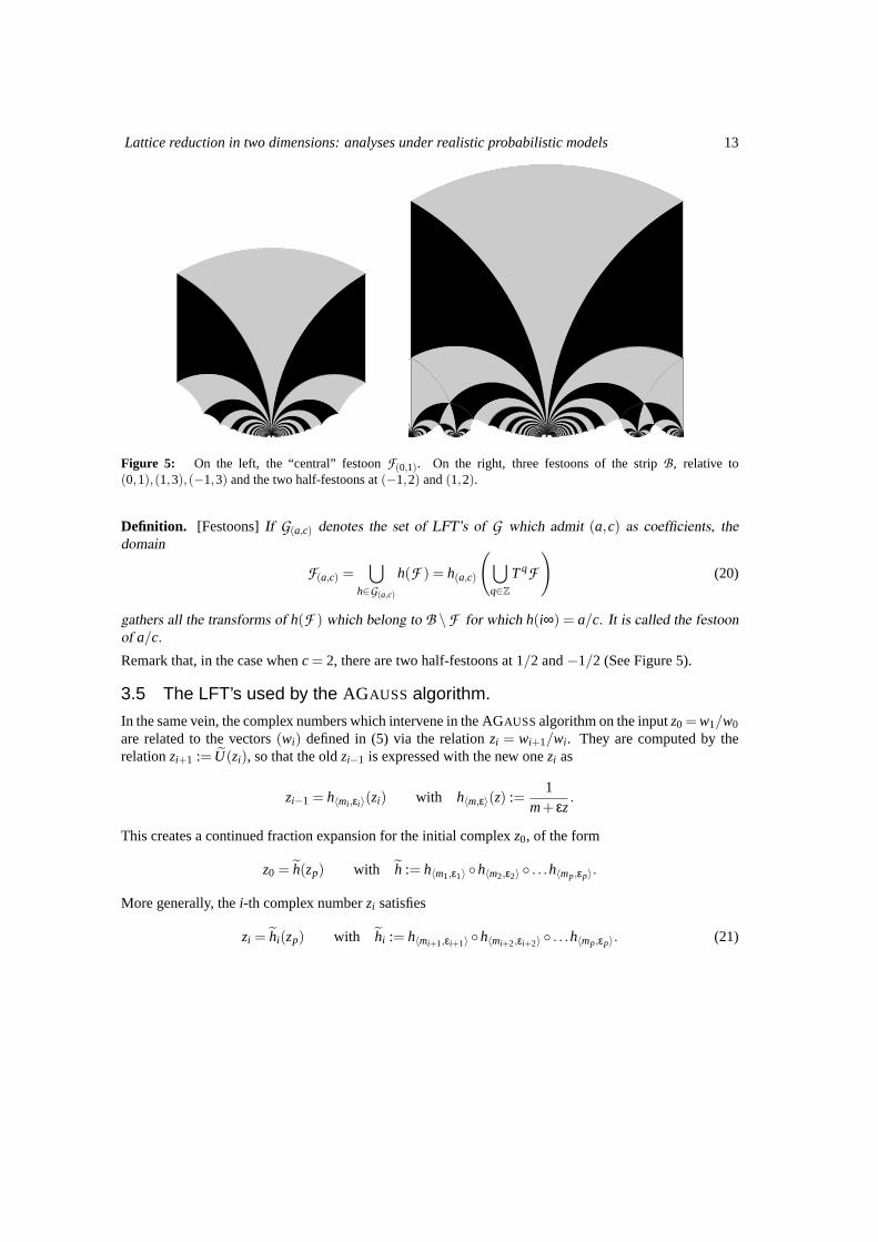
Figure 5: On the left, the “central” festoonF(0,1). On the right, three festoons of the stripB, relative to(0,1),(1,3),(−1,3) and the two half-festoons at(−1,2) and(1,2).

Definition. [Festoons]If G(a,c) denotes the set of LFT’s of G which admit (a,c) as coefficients, thedomain

F(a,c) =[

h∈G(a,c)

h(F ) = h(a,c)

([q∈Z

TqF

)(20)

gathers all the transforms of h(F ) which belong to B \F for which h(i∞) = a/c. It is called the festoonof a/c.

Remark that, in the case whenc = 2, there are two half-festoons at 1/2 and−1/2 (See Figure 5).

3.5 The LFT’s used by the AGAUSS algorithm.

In the same vein, the complex numbers which intervene in the AGAUSSalgorithm on the inputz0 = w1/w0

are related to the vectors(wi) defined in (5) via the relationzi = wi+1/wi . They are computed by therelationzi+1 := U(zi), so that the oldzi−1 is expressed with the new onezi as

zi−1 = h〈mi ,εi〉(zi) with h〈m,ε〉(z) :=1

m+ εz.

This creates a continued fraction expansion for the initial complexz0, of the form

z0 = h(zp) with h := h〈m1,ε1〉 h〈m2,ε2〉 . . .h〈mp,εp〉.

More generally, thei-th complex numberzi satisfies

zi = hi(zp) with hi := h〈mi+1,εi+1〉 h〈mi+2,εi+2〉 . . .h〈mp,εp〉. (21)


We now explain the particular role which is played by the diskD of diameterI = [0,1/2]. Figure 6 showsthat the domainB \D decomposes as the union of six transforms of the fundamental domainF , namely

B \ D =[

h∈Kh(F ) with K := I ,S,STJ,ST,ST2J,ST2JS. (22)

This shows that the diskD itself is also a union of transforms of the fundamental domainF . Remarkthat the situation is different for the PGAUSS algorithm, since the frontier ofD lies “in the middle” oftransforms of the fundamental domainF (see Figure 6).

D

ST 2JF+

STF−

STJF+

SF−

F+

ST 2JSF−

Figure 6: On the left, the six domains which constitute the domainB+ \D+. On the right, the diskD is notcompatible with the geometry of transforms of the fundamental domainsF .

As Figure 7 shows it, there are two main parts in the execution of the AGAUSS Algorithm, according tothe position of the current complexzi with respect to the diskD whose equation is

D := z; ℜ(

1z

)≥ 2.

While zi belongs toD, the quotient(mi ,εi) satisfies(mi ,εi) ≥ (2,+1) (wrt the lexicographic order), andthe algorithm uses at each step the set

H := h〈m,ε〉; (m,ε)≥ (2,+1)

so thatD can be written as

D =[

h∈H +

h(B \D) with H + := ∑k≥1

H k. (23)

The part of the AGAUSSalgorithm performed whenzi belongs toD is called the COREGAUSSalgorithm.The total set of LFT’s used by the COREGAUSS algorithm is then the setH + = ∪k≥1H k. As soon aszi


does not any longer belong toD, there are two cases. Ifzi belongs toF , then the algorithm ends. Ifzi

belongs toB \ (F ∪D), there remains at most two iterations (due to (22) and Figure 6), that constitutesthe FINAL GAUSS algorithm, which uses the setK of LFT’s, called the final set of LFT’s. Finally, wehave proven:

Proposition 3. The set G formed by the LFT’s which map the fundamental domain F into the set B \ Fdecomposes as G = (H ? ·K )\I where

H ? := ∑k≥0

H k, H := h〈m,ε〉; (m,ε)≥ (2,+1), K := I ,S,STJ,ST,ST2J,ST2JS.

Here, if D denotes the disk of diameter [0,1/2], then H + is the set formed by the LFT’s which map B \Dinto D and K is the final set formed by the LFT’s which map F into B \D . Furthermore, there is acharacterization of H + due to Hurwitz which involves the golden ratio φ = (1+

√5)/2:

H + := h(z) =az+bcz+d

; (a,b,c,d) ∈ Z4,b,d≥ 1,ac≥ 0,

|ad−bc|= 1, |a| ≤ |c|2

,b≤ d2,− 1

φ2 ≤cd≤ 1

φ.

COREGAUSS(z)

Input. A complex number inD.Output. A complex number inB \D.

While z∈ D do z := U(z);

FINAL GAUSS(z)

Input. A complex number inB \D.Output. A complex number inF .

While z 6∈ F do z := U(z);

AGAUSS(z)

Input. A complex number inB \ F .Output. A complex number inF .

COREGAUSS (z);FINAL GAUSS (z);

Figure 7: The decomposition of the AGAUSS Algorithm.

3.6 Comparing the COREGAUSS algorithm and the F-EUCLID algorithm.

The COREGAUSS algorithm has a nice structure since it uses at each step the same setH . This set isexactly the set of LFT’s which is used by the F-EUCLID Algorithm relative to the dynamical systemdefined in (18). Then, the COREGAUSS algorithm is just a lifting of this F-EUCLID Algorithm, whereasthe final steps of the AGAUSSalgorithm use different LFT’s, and are not similar to a lifting of a EuclideanAlgorithm. This is why the COREGAUSSalgorithm is interesting to study: we will see in Section 5.3 whyit can be seen as an exact generalization of the F-EUCLID algorithm.


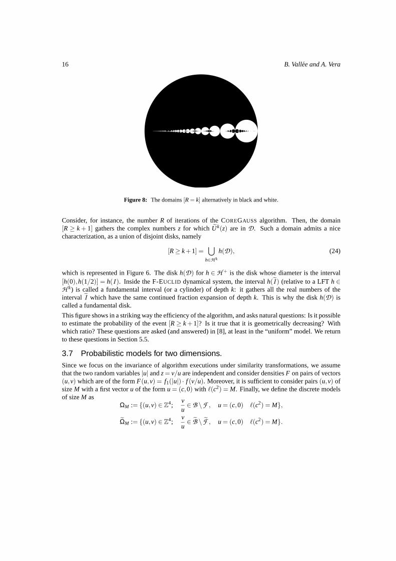
Figure 8: The domains[R= k] alternatively in black and white.

Consider, for instance, the numberR of iterations of the COREGAUSS algorithm. Then, the domain[R≥ k+ 1] gathers the complex numbersz for which Uk(z) are in D. Such a domain admits a nicecharacterization, as a union of disjoint disks, namely

[R≥ k+1] =[

h∈H k

h(D), (24)

which is represented in Figure 6. The diskh(D) for h ∈ H + is the disk whose diameter is the interval[h(0),h(1/2)] = h(I ). Inside the F-EUCLID dynamical system, the intervalh(I ) (relative to a LFTh∈H k) is called a fundamental interval (or a cylinder) of depthk: it gathers all the real numbers of theinterval I which have the same continued fraction expansion of depthk. This is why the diskh(D) iscalled a fundamental disk.

This figure shows in a striking way the efficiency of the algorithm, and asks natural questions: Is it possibleto estimate the probability of the event[R≥ k+ 1]? Is it true that it is geometrically decreasing? Withwhich ratio? These questions are asked (and answered) in [8], at least in the “uniform” model. We returnto these questions in Section 5.5.

3.7 Probabilistic models for two dimensions.Since we focus on the invariance of algorithm executions under similarity transformations, we assumethat the two random variables|u| andz= v/u are independent and consider densitiesF on pairs of vectors(u,v) which are of the formF(u,v) = f1(|u|) · f (v/u). Moreover, it is sufficient to consider pairs(u,v) ofsizeM with a first vectoru of the formu = (c,0) with `(c2) = M. Finally, we define the discrete modelsof sizeM as

ΩM := (u,v) ∈ Z4;vu∈ B \F , u = (c,0) `(c2) = M,

ΩM := (u,v) ∈ Z4;vu∈ B \ F , u = (c,0) `(c2) = M.


In both cases, the complexz= v/u belongs toQ[i] and is of the form(a/c)+ i(b/c). When the integersc andM tend to∞, this discrete model “tends” to a continuous model, and the densityf is defined on asubset ofC. It is sometimes more convenient to view this density as a function defined onR2, and wedenote byf the functionf viewed as a function of two real variablesx,y. It is clear that the roles of twovariablesx,y are not of the same importance: the variabley = ℑ(z) plays the crucial role, whereas thevariablex= ℜ(z) plays an auxiliary role. This is why the two main models that are now presented involvedensitiesf (x,y) which only depend ony.

Results of Akhavi [1] and Akhavi, Marckert, Rouault [2] show that densities “with valuation” play anatural role in lattice reduction algorithms. We are then led to consider the 2–dimensional bases(u,v)which follow the so–called model of valuationr (with r >−1), for which

P[(u,v);

|det(u,v)|max(|u|, |v|)2 ≤ y

]= Θ(yr+1), when y→ 0.

We note that, when the valuationr tends to−1, this model tends to the “one dimensional model”, whereu andv are colinear. In this case, the Gauss Algorithm “tends” to the Euclidean Algorithm, and it isimportant to precisely describe the transition. This model “with valuation” was already presented in [21]in a slightly different context, but not actually studied there.

The model with valuation defines a scale of densities, for which the weight of skew bases may vary. Whenr tends to−1, almost all the input bases are formed of vectors which form a very small angle, and, with ahigh probability, they represent hard instances for reducing the lattice.

In the complex framework, a densityf on the setS ⊂ C\R is of valuationr (with r >−1) if it is of theform

f (z) = |ℑ(z)|r ·g(z) where g(z) 6= 0 for ℑ(z) = 0. (25)

Such a density is called of type(r,g). We often deal with the standard density of valuationr,

fr(z) =1

A(r)|ℑ(z)|r with A(r) =

ZZB\F

yrdxdy. (26)

Of course, whenr = 0, we recover the uniform distribution onB \F with A(0) = (1/12)(2π + 3√

3).Whenr →−1, thenA(r) is Θ[(r +1)−1]. More precisely

A(r)− 1r +1

(√3

2

)r+1

= log43.

Notations. The (continuous) model relative to a densityf is denoted with an index of the form〈 f 〉, andwhen the valuation is the standard density of valuationr, the model is denoted with an index of the form(r). The discrete models are denoted by two indices, the integer sizeM and the index which describes thefunction f , as previously.

3.8 The LLL algorithm and the complex framework.Consider a lattice ofRn generated by a setB := b1,b2, . . . ,bn of n independent vectors. The LLLalgorithm “reduces” the basisB by successively dealing with two-dimensional latticesLk generated by


the so-called local basesBk: Thek-th local basisBk is formed with the two vectorsuk,vk, defined as theorthogonal projection ofbk,bk+1 on the orthogonal of the subspace〈b1,b2, . . . ,bk−1〉. The LLL algorithmis a succession of calls to the Gauss algorithm on these local bases, and it stops when all the local bases arereduced (in the Gauss meaning). Then, the complex output ˆzk defined from(uk, vk) as in (1) is an elementof the fundamental domainF . Figure 1 (on the right) shows the experimental distribution of outputs ˆzk,which does not seem to depend on indexk∈ [1..n]. There is an accumulation of points in the “corners” ofF , and the mean value of parameterγ is close to 1.04.

4 Analysis of the output parameters.This section describes the probabilistic behaviour of output parameters: we first analyze the output den-sities, then we focus on the geometry of our three main parameters defined in (11, 12). We shall use thePGAUSS Algorithm for studying the output parameters.

4.1 Output densities.For studying the evolution of distributions (on complex numbers), we are led to consider the 2–variablesfunctionh that corresponds to the complex mappingz 7→ h(z). More precisely, we consider the functionhwhich is conjugated to(v,w) 7→ (h(v),h(w)) with respect to mapΦ, namelyh = Φ−1 (h,h)Φ, wheremappingsΦ,Φ−1 are linear mappingsC2 → C2 defined as

Φ(x,y) = (z= x+ iy,z= x− iy), Φ−1(z,z) =(

z+z2

,z+z2i

).

SinceΦ andΦ−1 are linear mappings, the JacobianJhof the mappingh satisfies

Jh(x,y) = |h′(z) ·h′(z)|= |h′(z)|2, (27)

sinceh has real coefficients. Consider any measurable setA ⊂ F . The final densityf on A is brought byall the antecedentsh(A) for h∈ G , which form disjoints subsets ofB \F . Then,ZZ

Af (x, y)dxdy = ∑

h∈G

ZZh(A)

f (x,y)dxdy.

Using the expression of the Jacobian (27), and interverting integral and sum lead to

∑h∈G

ZZA|h′(z)|2 f h(x, y)dxdy =

ZZA

(∑

h∈G|h′(z)|2 f h(x, y)

)dxdy.

Finally, we have proven:

Theorem 1. (i)The output density f on the fundamental domain F can be expressed as a function of theinput density f on B \F as

f (x, y) = ∑h∈G

|h′(z)|2 f h(x, y),

where G is the set of LFTs used by the PGAUSS algorithm defined in Proposition 2.


(ii) In the same vein, the output density f on the fundamental domain F can be expressed as a functionof the input density f on B \ F as

f (x, y) = ∑h∈G

|h′(z)|2 f h(x, y),

where G is the set of LFTs used by the AGAUSS algorithm defined in Proposition 3.(iii ) Finally, the output density f on the domain B \D can be expressed as a function of the input densityf on D as

f (x, y) = ∑h∈H +

|h′(z)|2 f h(x, y),

where H is the set of LFTs used by the COREGAUSS algorithm defined in Proposition 3.

4.2 The irruption of Eisenstein series.

We now analyze an important particular case, where the initial density is the standard density of valuationr defined in (26). Since each element ofG gives rise to a unique pair(c,d) with c≥ 1,gcd(c,d) = 1 forwhich

|h′(z)|= 1|cz+d|4

, fr h(x, y) =1

A(r)yr

|cz+d|2r , (28)

the output density onF is fr(x, y) =1

A(r) ∑(c,d)=1

c≥1

yr

|cz+d|4+2r . (29)

It is natural to compare this density to the density relative to the measure relative to “random lattices”: inthe particular case of two dimensions, the setX2 = SL2(R)/SL2(Z) is exactly¶ the fundamental domainF . Moreover, the measure of densityℑ(z)−2 is invariant under the action ofPSL2(Z): indeed, for anyLFT h with deth =±1, one has

|ℑ(h(z))|= |ℑ(z)| · |h′(z)|, so thatZZ

h(A)

1y2 dxdy=

ZZA|h′(z)|2 1

ℑ(h(z))2 dxdy=ZZ

A

1y2 dxdy.

Then, the probabilityν2 on F of density‖

η(x,y) :=3π

1y2 (30)

is invariant under the action ofPSL2(Z). If we make apparent this densityη inside the expression offrprovided in (29), we obtain:

Theorem 2. When the initial density on B \F is the standard density of valuation r , denoted by fr anddefined in (26), the output density of the PGAUSS algorithm on F involves the Eisenstein series Es of

¶ Not exactly: up to a convenient definition ofF on its frontier.‖ the integral

RRF η(x,y)dxdy= 1.


weight s= 2+ r: With respect to the Haar measure µ on F , whose density η is defined in (30), the outputdensity fr is expressed as

fr(x,y)dxdy=π

3A(r)F2+r(x,y)η(x,y)dxdy, where Fs(x,y) = ∑

(c,d)=1c≥1

ys

|cz+d|2s .

is closely related to the classical Eisenstein series Es of weight s, defined as

Es(x,y) :=12 ∑

(c,d)∈Z2

(c,d)6=(0,0)

ys

|cz+d|2s = ζ(2s) · [Fs(x,y)+ys] .

When r →−1, classical results about Eisenstein series prove that

Es(x,y)∼s→11

2(s−1)so that lim

r→−1

π3A(r)

F2+r(x,y) = 1,

which imply that the ouput distribution relative to the input distribution of valuation r tends to the distri-bution ν2 relative to random lattices when r →−1.

The seriesEs are Maass forms (see for instance the book [5]): they play an important role in the theory ofmodular forms, becauseEs is an eigenfunction for the Laplacian, relative to the eigenvalues(1−s). Theirruption of Eisenstein series in the lattice reduction framework was unexpected, and, at the moment, it isnot clear how to use the classical well-known properties of the Eisenstein seriesEs for studying the outputdensities.

4.3 Geometry of the output parameters.The main output parameters are defined in (11,12). ForX ∈ λ,µ,γ, we denote byX(z) the value ofXon basis(1,z), and there are close relations betweenX(u,v) andX(z) for z= v/u:

λ(u,v) = |u| ·λ(z), µ(u,v) = |u| ·µ(z), γ(u,v) = γ(z).

Moreover, the complex versions of parametersλ,µ,γ can be expressed with the input–output pair(z, z).

Proposition 4. If z= x+ iy is an initial complex number of B \F leading to a final complex z= x+ iyof F , then the three main output parameters defined in (11,12) admit the following expressions

detL(z) = y, λ2(z) =yy, µ2(z) = yy, γ(z) =

1y.

Then, the following inclusions hold:

[λ(z) = t]⊂

[ℑ(z)≥

√3

2t2

], [µ(z) = u]⊂

[ℑ(z)≤ 2√

3u2]. (31)

If z leads to z by using the LFT h∈ G with z= h(z) = (az+b)/(cz+d), then:

λ(z) = |cz−a|, γ(z) =|cz−a|2

y, µ(z) =

y|cz−a|

.


Fo(a,c,ρ) := (x,y); y > 0,(

x− ac

)2+(

y− ρ2c2

)2≤ ρ2

4c4

Fa(a,c, t) := (x,y); y > 0,(

x− ac

)2+y2 ≤ t2

c2

Se(a,c,u) := (x,y); y > 0, |y| ≤ cu√1−c2u2

∣∣∣x− ac

∣∣∣ for cu≤ 1

Se(a,c,u) := (x,y); y > 0, for cu≥ 1

Figure 9: The three main domains of interest: the Ford disksFo(a,c,ρ), the Farey disksFa(a,c, t), the angular sectorsSe(a,c,u).

Proof. If the initial pair (v1,v0) is written as in (4) as(v1

v0

)= M −1

(vp+1

vp

), with M −1 :=

(a bc d

)and z= h(z) =

az+bcz+d

,

then the total length decrease satisfies

|vp|2

|v0|2=

|vp|2

|cvp+1 +dvp|2=

1|cz+d|2

= |h′(z)|, (32)

[we have used the fact that detM = 1.] This proves thatλ2(z) equals|h′(z)| as soon asz= h(z). Now, forz= h(z), the relations

y =y

|cz+d|2, y =

y|cz−a|2

,

easily lead to the end of the proof.

4.4 Domains relative to the output parameters.

We now consider the following well-known domains defined in Figure 9. The Ford diskFo(a,c,ρ) is adisk of center(a/c,ρ/(2c2)) and radiusρ/(2c2): it is tangent toy = 0 at point(a/c,0). The Farey diskFa(a,c, t) is a disk of center(a/c,0) and radiust/c. Finally, the angular sectorSe(a,c,u) is delimited bytwo lines which intersect ata/c, and form with the liney= 0 angles equal to±arcsin(cu). These domainsintervene for defining the three main domains of interest.

Theorem 3. The domains relative to the main output parameters, defined as

Γ(ρ) := z∈ B \F ; γ(z)≤ ρ, Λ(t) := z∈ B \F ; λ(z) ≤ t,

M(u) := z∈ B \F ; µ(z) ≤ u


are described with Ford disks Fo(a,c,ρ), Farey disks Fa(a,c, t), and angular sectors Se(a,c,u). Moreprecisely, if F(a,c) denotes the Festoon relative to pair (a,c) defined in (20) and if the set C is defined asin (19), one has:

Γ(ρ) =[

(a,c)∈CFo(a,c,ρ)∩F(a,c), Λ(t) =

[(a,c)∈C

Fa(a,c, t)∩F(a,c),

M(u) =[

(a,c)∈CSe(a,c,u)∩F(a,c).

Each “local” definition of setsΛ,Γ,M can be transformed in a “global definition” which no more involvesthe festoons. It involves, for instance, a subfamily of complete (intersecting) Farey disks (forΛ), orquadrilaterals (forM) [see Figure 10].Define the subsetP (t) of setP defined in Section 3.4 as

P (t) := (c,d); c,d≥ 1,ct ≤ 1,dt ≤ 1,(c+d)t > 1,(c,d) = 1,

and, for a pair(a/c,b/d) of rationals satisfyingad−bc=−1, denote byS(a/c,b/d) the intersection ofB \F with the vertical strip(a/c)≤ x≤ (b/d).

The “global” definition of domainΛ(t) is provided in [12]: consider a pair(a/c,b/d) of rationals satisfy-ing ad−bc=−1 whose denominator pair(c,d) belongs toP (t). There exists a local characterization ofΛ(t)∩S(a/c,b/d) which does not depend any longer on the festoons, namely

Λ(t)∩S(a/c,b/d) = Fa+(a,c, t)∪Fa−(b,d, t)∪Fa(a+b,c+d, t). (33)

Here Fa+(a,c, t),Fa−(b,d, t) are the half Farey disks formed with the intersections ofFa(a,c, t),Fa(b,d, t) with the stripS(a/c,b/d). The domain of (33) is exactly the union of the two disksFa+(a,c, t)andFa−(b,d, t) if and only if the condition(c2 + d2 + cd)t2 > 1 holds. The Farey disk relative to themedian(a+ b)/(c+ d) only plays a role when(c2 + d2 + cd)t2 ≤ 1. This last condition is satisfied inparticular if max(ct,dt) is smaller than 1/

√3, or, equivalently, when bothc andd belong to the interval

[0,1/(t√

3)]. Whent → 0, the proportion of pairs(a/c,b/d) for which the intersection of Eqn (33) isformed with three disks tends to 1/6.

Then the following inclusions hold (where the “left” union is a disjoint union)[(a,c)∈Cc≤1/t

Fa(a,c, t)⊂ Λ(t)⊂[

(a,c)∈Cc≤2/(

√3t)

Fa(a,c, t). (34)

We now deal with the domainM(u): consider a pair(a/c,b/d) of rationals satisfyingad−bc=−1 whosedenominator pair(c,d) belongs toP (u). Then, the denominatorf of any rationale/ f of the interval]a/c,b/d[ satisfiesf u≥ (c+d)u > 1, and the domainSe(e, f ,u)∩F(e, f ) equals the whole festoonF(e, f ).We obtain a characterization ofM(u) which does not depend any longer on the festoons, namely

M(u)∩S(a/c,b/d) = Se(a,c,u)∩Se(b,d,u)∩Se(b−a,d−c,u). (35)


0 12

0 12

0.33333 0.40.250.2

0 12

13

14

15

16

17

18

25

37

38

27

Figure 10: On the top: the domainΓ(ρ) := z; γ(z)≤ ρ. On the left,ρ = 1 (in white). On the right,the festoonF(0,1) together withFo(0,1,ρ) for ρ = 1,ρ0 = 2/

√3,ρ1 = (1+ρ0)/2. – On the middle, the

domainΛ(t)∩B+, with Λ(t) := z; λ(z)≤ t for t = 0.193 andt = 0.12. – On the bottom, the domainM(u)∩B+ with M(u) := z; µ(z)≤ u for u = 0.193 andu = 0.12.


The domain of (35) may coincide with the triangleSe(a,c,u)∩ Se(b,d,u) when the two sides of thetriangle intersect on the frontierF(a,c) ∩F(b,d). But, this is not always the case since the two sides ofthe triangle may intersect inside the festoonF(b−a,d−c). In this case, the domain of (35) is a “true”quadrilateral. This last case occurs if and only if the condition(c2 + d2− cd)u2 ≥ (3/4) holds. Thiscondition is satisfied in particular if min(cu,du) is larger than

√3/2. This occurs in the interval[a/c,b/d]

when bothc andd belong to[(√

3/2)(1/u),1/u]. Whenu→ 0, the proportion of pairs(a/c,b/d) forwhich the intersection of Eqn (35) is a “true” quadrilateral tends to 2[1− (

√3/2)]2.

4.5 Distribution functions of output parameters.Computing the measure of disks and angular sectors with respect to a standard density of valuationr leadsto the estimates of the main output distributions:

Theorem 4. When the initial density on B \F is the standard density of valuation r , the three mainoutput parameters admit the following distributions:

P(r)[γ(z)≤ ρ] = A1(r) ·ζ(2r +3)ζ(2r +4)

·ρr+2 for ρ ≤ 1,

P(r)[λ(z)≤ t] = Θ(tr+2) for r > 0,P(r)[λ(z)≤ t] = Θ(t2| logt|) for r = 0,P(r)[λ(z)≤ t] = Θ(t2r+2) for r < 0,

P(r)[µ(z)≤ u] = Θ(u2r+2).

In the case when r ≥ 0, there are precise estimates for parameter λ, when t → 0:

P(r)[λ(z)≤ t] ∼t→0 A2(r)ζ(r +1)ζ(r +2)

· tr+2 for r > 0,

P(r)[λ(z)≤ t] ∼t→0 A2(0)1

ζ(2)t2| logt| for r = 0.

For any valuation r >−1, the following inequalities hold

P(r)[λ(z)≤ t]≥ 1A(r)

1r +1

(√3

2

)r+1

t2r+2, P(r)[µ(z)≤ u]≤ A3(r)(

2√3

)r+1

u2r+2.

The constants Ai(r) involve Euler’s Gamma function and the measure A(r) defined in (26) in the followingway

A1(r) :=√

πA(r)

Γ(r +3/2)Γ(r +3)

, A2(r) =√

π2A(r)

Γ((r +1)/2)Γ(r/2+2)

, A3(r) =1

A(r)1

(r +2)(r +1).

Proof. [Sketch] First, the measure (wrt the standard density of valuationr) of each basic domain (disksof Farey or Ford type, triangles) is easy to compute. For a disk of radiusρ, centered on the real axis (resp


tangent to the real axis), this measure equals 2A2(r)ρr+2 (resp. A1(r)(2ρ)r+2), and involves constantsAi(r) defined in the theorem. Furthermore, ifϕ denotes the Euler totient function, there are exactlyϕ(c)basic disks of the same radius in each domain. Then, the identity

∑c≥1

ϕ(c)cs =

ζ(s−1)ζ(s)

, for ℜs≥ 2

explains the occurrence of the functionζ(s−1)/ζ(s) in our estimates. Consider two examples:

(a) Forρ≤ 1, the domainΓ(ρ) is made with disjoint Ford disks of radiusρ/(2c2). An easy applicationof previous principles leads to the result.

(b) For Λ(t), these same principles, together with relation (34) entail the following inequalities

tr+2 ∑c≤1/t

ϕ(c)cr+2 ≤ 1

A2(r)P(r)[λ(z)≤ t]≤ tr+2 ∑

c≤2/(√

3t)

ϕ(c)cr+2 ,

and there are several cases whent → 0 according the sign ofr. Forr > 0, the Dirichlet series involved areconvergent. Forr ≤ 0, we consider the series

∑c≥1

ϕ(c)cr+2+s =

ζ(s+ r +1)ζ(s+ r +2)

,

(which has a pole ats=−r), and Tauberian theorems (or Perron’s formula forr = 0) provide an estimatefor

∑c≤N

ϕ(c)cr+2 ∼N→∞

1ζ(2)

Nr+1, (for r > 0), and ∑c≤N

ϕ(c)c2 ∼N→∞

1ζ(2)

N logN.

For domainM(u), the study of quadrilaterals can be performed in a similar way. The measure (wrtstandard density of valuationr) of a triangle of horizontal basisa and heighth is of the formA3(r)ahr+1,and involves the constantA3(r) defined in the theorem. Furthermore, the height of each quadrilateral ofM(u) is Θ(u2), and the sum of the basesa equal 1. ThenP(r)[µ(z) ≤ u] = Θ(u2r+2). Furthermore, usingthe inclusions of (31) leads to the inequality.

Interpretation of the results. We provide a first interpretation of the main results described in the previ-ous theorem.

(i) For anyy0 ≥ 1, the probability of the event[y≥ y0] is

P(r)[y≥ y0] = P(r)[γ(z)≤1y0

] = A1(r)ζ(2r +3)ζ(2r +4)

1

yr+20

.

This defines a function of the variabley0 7→ ψr(y0), whose derivative is a power function of variabley0,of the formΘ(y−r−3

0 ). This derivative is closely related to the output densityfr of Theorem 2, via theequality

ψ′r(y0) :=

Z +1/2

−1/2fr(x,y0)dx.


Now, whenr →−1, the functionψ′r(y) has a limit which is exactly the densityη, defined in (30), which

is associated to the Haar measureµ2 defined in 7.2.

(ii) The regime of the distribution function of parameterλ changes when the sign of valuationr changes.There are two parts in the domainΛ(t): the lower part, which is the horizontal strip[0≤ℑ(z)≤ (2/

√3)t2],

and the upper part defined as the intersection ofΛ(t) with the horizontal strip[(2/√

3)t2 ≤ ℑ(z)≤ t]. Fornegative values ofr, the measure of the lower part is dominant, while, for positive values ofr, this is theupper part which has a dominant measure. Forr = 0, there is a phase transition between the two regimes:this occurs in particular in the usual case of a uniform density.

(iii ) In contrast, the distribution function of parameterµ has always the same regime. In particular, fornegative values of valuationr, the distribution functions of the two parameters,λ andµ are of the sameform.

Open questions.Is it possible to get information on the constants hidden in theΘ’s for parameterµ (incase of any valuation) and forλ (in case of a negative valuation)? This will be important in the study ofthe LLL algorithm (See Section 4.7).

Is it possible to describe the distribution function of parameterρ for ρ > 1? Figure 10 [top] shows that itsregime changes atρ = 1. This will be important for obtaining a precise estimate of the mean valueE(r)[γ]as a function ofr and comparing this value to experiments reported in the Introduction.

4.6 The corners of the fundamental domainWith Theorem 4, it is possible to compute the probability that an output basis lies in the corners of thefundamental domain, and to observe its evolution as a function of valuationr. This is a first step for asharp understanding of Figure 1[right].

Proposition 5. When the initial density on B \F is the standard density of valuation r , the probabilityfor an output basis to lie on the corners of the fundamental domain is equal to

C(r) := 1−A1(r) ·ζ(2r +3)ζ(2r +4)

.

There are three main cases of interest for 1−C(r)

[r →−1] :3π

[r = 0] :3π

2π+3√

3

ζ(3)ζ(4)

[r → ∞] :

√πr

e−3/2.

4.7 Returning to the LLL Algorithm.The LLL algorithm aims at reducing all the local basesBk in the Gauss meaning. For obtaining the outputdensity at the end of the algorithm, it is interesting to describe the evolution of the distribution of the localbases along the execution of the algorithm.

There exists for instance a variant of the LLL algorithm, introduced by Villard [23] which performs asuccession of phases of two types, the odd ones, and the even ones. We adapt this variant and choose toperform the AGAUSSalgorithm, because, as we shall explain in Section 6, it has a better structure. Duringone even (resp. odd) phase, thewholeAGAUSS algorithm is performed on all local basesBk with even


(resp. odd) indices. Since local bases with odd (resp. even) indices are “disjoint”, it is possible to performthese Gauss algorithmsin parallel. This is why Villard has introduced this algorithm.Consider the Odd phase, and two successive basesBk andBk+2 with odd indices, respectively endowedwith some initial densitiesFk andFk+2. Denote byzk andzk+2 the complex numbers associated to localbases(uk,vk) and(uk+2,vk+2) via relation (1). Then, the LLL algorithm reduces these two local bases (inthe Gauss meaning) and computes two reduced local bases denoted by(uk, vk) and(uk+2, vk+2), whichsatisfy in particular

|v?k|= |uk| ·µ(zk), |uk+2|= |uk+2| ·λ(zk+2).

Then our Theorem 4 provides insights on the distribution ofµ(zk),λ(zk+2). Since, in our model, therandom variables|uk| andzk (resp.|uk+2| andzk+2) are independent, we obtain a precise information onthe distribution of the norms|v?

k|, |uk+2|.In the Even phase, the LLL algorithm considers the local bases with an odd index. Now, the basisBk+1 isformed (up to a similarity) from the two previous output bases, as:

uk+1 = |v?k|, vk+1 = ν|v?

k|+ i|uk+2|,

whereν can be assumed to follow a uniform law on[−1/2,+1/2]. Moreover, at least at the beginning ofthe algorithm, the two variables|v?

k|, |uk+2| are independent. All this allows to obtain precise informationson the new input densityFk+1 of the local basisBk+1. We then hope to “follow” the evolution of densitiesof local bases along the execution of the LLL algorithm.

5 Analysis of the execution parameters.We finally focus on parameters which describe the execution of the algorithm: we are mainly interestedin the bit–complexity, but we also study additive costs that may be of independent interest. We here usean approach both based on tools that come from dynamical system theory and analysis of algorithms. Weshall use here the AGAUSS algorithm, with the decomposition provided in Proposition 3.

5.1 Dynamical systems and transfer operators.Recall that a dynamical system is a pair formed by a compact setX and a mappingW : X → X for whichthere exists a (finite or denumerable) setQ , (whose elements are called digits), and a topological partitionXqq∈Q of the setX in subsetsXq such that the restriction ofW to each elementXq of the partition isC2 and invertible. Here, we are led to so–called complete dynamical systems, where the restriction ofW|Xq : Xq → X is surjective. A special role is played by the setH of branches of the inverse functionW−1

of W that are also naturally numbered by the index setQ : we denote byh〈q〉 the inverse of the restrictionW|Xq, so thatXq is exactly the imageh〈q〉(X). The setH k is the set of the inverse branches of the iterateWk; its elements are of the formh〈q1〉 h〈q2〉 · · ·h〈qk〉 and are called the inverse branches of depthk. ThesetH ? := ∪k≥0H k is the semi-group generated byH .

Given an initial pointx in X, the sequenceW (x) := (x,Wx,W2x, . . .) of iterates ofx under the action ofWforms the trajectory of the initial pointx. We say that the system has a holeY if any point ofX eventuallyfalls in Y: for anyx, there existsp∈ N such thatWp(x) ∈Y.

The main study in dynamical systems concerns itself with the interplay between properties of the trans-formationW and properties of trajectories under iteration of the transformation. The behaviour of typical


trajectories of dynamical systems is more easily explained by examining the flow of densities. The timeevolution governed by the mapW modifies the density, and the successive densitiesf1, f2, . . . , fn, . . . de-scribe the global evolution of the system at timet = 0, t = 1, t = 2, . . ..We will study here two dynamical systems, respectively related to the F-EUCLID algorithm and to CORE-GAUSS algorithm, and defined in Sections 3.3 and 3.5.

5.2 Case of the F-EUCLID system.We first focus on the case whenX is a compact interval of the real line. Consider the (elementary) operatorX2s,[h], relative to a mappingh, which acts on functionsf of one variable, depends on some parametersand is formally defined as

Xs,[h][ f ](x) = |h′(x)|s · f h(x). (36)

The operatorX1,[h] expresses the part of the new density which is brought when one uses the branchh,and the operator

Hs := ∑h∈H

Hs,[h] (37)

is called the transfer operator. Fors= 1, the operatorH1 = H is the density transformer, (or the Perron-Frobenius operator) which expresses the new densityf1 as a function of the old densityf0 via the relationf1 = H[ f0]. In the case of the F-EUCLID algorithm, due to the precise expression of the setH , one has,for anyx∈ I = [0,1/2]

Hs[ f ](x) = ∑(m,ε)≥(2,1)

(1

m+ εx

)2s

· f

(1

m+ εx

).

The density transformerH admits a unique invariant densityψ(x) which involves the golden ratioφ =(1+

√5)/2,

ψ(x) =1

logφ

(1

φ+x+

1φ2−x

).

This is the analog (for the F-EUCLID algorithm) of the celebrated Gauss density associated to the standardEuclid algorithm and equal to(1/ log2)1/(1+x).

The main properties of the F-EUCLID algorithm are closely related to spectral properties of the transferoperatorHs, when it acts on a convenient functional space. We return to this fact in Section 5.4.

5.3 Case of the AGAUSS algorithm.Theorem 1 describes the output densityf as a function of the initial densityf . The output densityf (z)is written as a sum of all the portions of the density which are brought by all the antecedentsh(z), whenh∈ G . We have seen in the proof of this theorem that the Jacobian of the transformation(x,y) 7→ h(x,y) =h(x+ iy) intervenes in the expression off as a function off . Furthermore, the JacobianJh(x,y) is equalto |h′(z)]2. It would be natural to consider an (elementary) operatorY2s,[h], of the form

Y2s,[h][ f ](z) = |h′(z)|2s · f (h(z)).

In this case, the sum of such operators, taken over all the LFT’s which intervene in one step of the AGAUSS

algorithm, and viewed ats= 1, describes the new density which is brought at each pointz∈ F during


this step, when the density onB \ F is f . However, such an operator has not good properties, because themodulus|h′(z)| does not define an analytic function. It is more convenient to introduce another elementaryoperator which acts on functionsF of two variables, namely

X2s,[h][F ](z,u) = h(z)s · h(u)s ·F(h(z),h(u)),

whereh is the analytic extension of|h′| to a complex neighborhood of[0,1/2]. Such an operator acts onanalytic functions, and the equalities

X2s,[h][F ](z,z) = Y2s,[h][ f ](z), X2s,[h][F ](x,x) = X2s,[h][ f ](x) for f (z) := F(z,z), (38)

prove that the elementary operatorsX2s,[h] are extensions of the operatorsX2s,[h] that are well-adapted toour purpose. Furthermore, they are also well-adapted to deal with densities with valuation. Indeed, whenapplied to a densityf of valuationr, of the form f (z) = F(z,z), whenF(z,u) = |z−u|rL(z,u) involves ananalytic functionL which is non zero on the diagonalz= u, one has

X2s[F ](z,z) = |y|rX2s+r [L](z,z).

Such operators satisfy a crucial relation of composition: with multiplicative properties of the derivative ofgh, we easily remark that

Xs,[h] Xs,[g] = Xs,[gh].

Then, the operators relative to the main set of LFT’sG ,K ,H associated to the AGAUSS algorithm viaProposition 3, defined as

Hs := ∑h∈H

Xs,[h], Ks := ∑h∈K

Xs,[h] Gs := ∑h∈G

Xs,[h], (39)

satisfy with Proposition 3,Gs = Ks (I −Hs)

−1− I . (40)

Remark that the operatorH2s admits the nice expression

H2s[F ](z,u) = ∑(m,ε)≥(2,1)

(1

(m+ εz)(m+ εu)

)2s

·F(

1m+ εz

,1

m+ εu

).

Due to (38), this is an extension ofH2s (defined in (37), which satisfies relationH2s[F ](x,x) = H2s[ f ](x)when f is the diagonal map ofF . Furthermore, assertions(ii) and(iii ) of Theorem 1 can be re–written as:Consider the densities (the input density f and the output density f ) as functions of two complex variablesz,z, namely f (x,y) = F(z,z), f (x,y) = F(z,z). Then

(Assertion (ii)): F = G2[F ], (Assertion (iii )): F = H2 (I −H2)−1[F ]

and the operators G2, H2 (I −H2)−1 can be viewed as (total) “density transformers” of the algorithms(the AGAUSS algorithm or the COREGAUSS algorithm) since they describe how the final density F canbe expressed as a function of the initial density F .


The operators defined in (39) are called transfer operators. Fors= 1, they coincide with density trans-formers, and, for other values ofs, they can be wiewed as extensions of density transformers. They playa central role in studies of dynamical systems. The main idea in “dynamical analysis” methodology isto use these operatorsX2s,[h] and to modify them in such a way that they become “generating operators”that generate themselves generating functions of interest. For instance, if a costc(h) is defined for themappingh, it is natural to add a new parameterw for marking the cost, and consider the weighted operatorXs,w,(c),[h] defined as

X2s,w,(c),[h][F ](z,u) = exp[wc(h)] · h(z)s · h(u)s ·F(h(z),h(u)).

Of course, whenw = 0, we recover the operatorX2s,[h]. When the costc is additive, i.e.,c(g h) =c(g)+c(h), the composition relation

Xs,w,(c),[h] Xs,w,(c),[g] = Hs,w,(c),[gh]

entails, with Proposition 3, an extension of (40) as

Gs,w,(c) = Ks,w,(c) (I −Hs,w,(c))−1− I (41)

5.4 Functional analysis.

It is first needed to find a convenient functional space where the operatorHs and its variantsHs,w,(c) willpossess good spectral properties : Consider the open diskV of diameter[−1/2,1] and the functional spaceB∞(V ) of all functionsF (of two variables) that are holomorphic in the domainV ×V and continuouson the closureV ×V . Endowed with the sup-norm,

||F ||= sup|F(z,u)|; (z,u) ∈ V ×V ,

B∞(V ) is a Banach space and the transfer operatorHs acts onB∞(M ) for ℜ(s) > (1/2) and is compact.

Furthermore, when weighted by a cost of moderate growth [i.e.,c(h〈q〉) = O(logq)], for w close enoughto 0, andℜs> (1/2), the operatorHs,w,(c) also acts onB∞(V ). Moreover, (see [22], [6]), for a complexnumbersclose enough to the real axis, withℜs> (1/2), it possesses nice spectral properties; in particular,in such a situation, the operatorHs,w,(c) has a unique dominant eigenvalue(UDE), denoted byλ(c)(s,w),which is separated from the remainder of the spectrum by a spectral gap(SG). This implies the following:for any fixeds close enough to the real axis, the quasi–inversew 7→ (I −Hs,w,(c))−1 has a dominant polelocated atw = w(c)(s) defined by the implicit equationλ(c)(s,w(c)(s)) = 1. In particular, whenw = 0, onehas:

(I −Hs)−1[F ](z,u) =

1s−1

6logφπ2 ψ(z,u)

ZI

F(x,x)dx, (42)

whereψ(x) is an extension of the invariant densityψ, and satisfiesψ(x,x) = ψ(x). An exact expressionfor ψ is provided in [22],

ψ(z,u) =1

logφ1

u−z

(log

φ+uφ+z

+ logφ2−uφ2−z

)for z 6= u, and ψ(z,z) = ψ(z).


5.5 Additive costs.We recall that we wish to analyze the additive costs described in Section 2.3. and defined more preciselyin (9). Such a costC(c) is defined via an elementary costc defined on quotientsqi , and we are interested byelementary costs of moderate growth, for whichc(|q|) = O(log|q|). Such costs will intervene in the studyof the bit–complexity cost, and will be relative in this case to the elementary costc(|q|) := `(|q|) where`(x) denotes the binary length of the integer cost. There is another important case of such an additive cost:the number of iterations, relative to an elementary costc = 1.

We first note thatc can be defined on LFT’sh corresponding to one step of the algorithm, via the relationc(h〈q,ε〉) := c(q); and then it can be extended to the total set of LFT’s in a linear way: forh = h1 h2 . . .hp, we definec(h) asc(h) := c(h1)+c(h2)+ . . .+c(hp). This gives rise to another definition for the

complex version of the cost defined byC(z) := C(1,z). If z∈ B \ F leads to ˆz∈ F by using the LFTh∈ G with z= h(z), thenC(z) equals (by definition)c(h).

We study costC(c) in the continuous∗∗ model relative to a densityf of type (r,g) defined in (25), andwe wish to prove thatk 7→ P〈 f 〉[C(c) = k] has a geometrical decreasing, with an estimate of the ratio. Forthis purpose, we use the moment generating function of the costC(c), denoted byE〈 f 〉(exp[wC(c)]) whichsatisfies

E〈 f 〉(exp[wC(c)]) := ∑k≥0

exp[wk] ·P[C(c) = k] = ∑h∈G

exp[wc(h)]ZZ

h(F )f (x,y)dxdy.

When the density is of the form (25), using a change of variables, the expression of the Jacobian, andrelation (28) leads to

E〈 f 〉(exp[wC(c)]) = ∑h∈G

exp[wc(h)]ZZ

Fyr |h′(z)|2+rg(h(z),h(z))dxdy.

This expression involves the transfer operatorG2+r,w,(c) of the algorithm AGAUSS, and with (41),

E〈 f 〉(exp[wC(c)]) =ZZ

Fyr [K2+r,w (I −H2+r,w)−1− I

][g](z,z)dxdy.

The asymptotic behaviour ofP[C(c) = k] is obtained by extracting the coefficient of exp[kw] in the moment

generating function. This series has a pole atew(2+r) for the valuew(2+ r) of w defined by the spectralequationλ(c)(2+r,w(2+r)) = 1 that involves the dominant eigenvalue of the core operatorHs,w,(c). Then,with classical methods of analytical combinatorics, we obtain:

Theorem 5. Consider a step-cost c of moderate growth, namely c : N → R+ with c(q) = O(log(q)) andthe relative additive cost C(c) defined in (9). Then, for any density f of valuation r , the cost C(c) followsan asymptotic geometric law. Moreover, the ratio of this law is closely related to the dominant eigenvalueof the core transfer operator Hs,w,(c), via the relation

P〈 f 〉[C(c) = k]∼ a(r)exp[−kw(c)(2+ r)], for k→ ∞, (43)

∗∗ It is also possible to transfer this continuous model to the discrete one. This is done for instance in [8].


where a(r) is some strictly positive constant which depends on density f and cost c. The ratio w(c)(2+ r)is defined by the spectral relation λ(c)(2+ r,w(2+ r)) = 1; it only depends on cost c and the valuation r ,not on the density itself, and satisfies w(c)(2+ r) = Θ(r +1) when r →−1.

In the particular case of a constant step-costc equal to 1, the operatorHs,w,(1) is simplyew ·Hs, and thevaluew(1)(s) is defined by the the relationewλ(s) = 1: this entails that the ratio in (43) is just equal toλ(2+ r). We recover in this case the main results of [8, 22].In this case, there exists an alternative expression for the mean number of iterations of the COREGAUSS

algorithm which uses the characterization of Hurwitz (recalled in Proposition 3). Furthermore, the prob-ability of the event[R≥ k+1] can be expressed in an easier way using (24), as

P[R≥ k+1] =1

A3(r)∑

h∈H k

ZZh(D)

yrdxdy=1

A3(r)

ZZD

(∑

h∈H k

|h′(z)|2+r)yrdxdy

=1

A4(r)

ZZD

yr Hk2+r [1](z)dxdy,

whereA4(r) is the measure ofD with respect to the standard density of valuationr,

A4(r) =√

π4r+2

Γ((r +1)/2)Γ(r/2+2)

. (44)

This leads to the following result:

Theorem. [Daude, Flajolet, Vallee]Consider the continuous model with the standard density of valuationr . Then, the expectation of the number of iterations Rof the COREGAUSS algorithm admits the followingexpression

E(r)[R] =1

A4(r)

ZZD

yr(I −H2+r)−1[1](z,z)dxdy=

22+r

ζ(2r +4) ∑(c,d)

dφ<c<dφ2

1(cd)2+r .

Furthermore, for any fixed valuation r >−1, the number of iterations follows a geometric law

P(r)[R≥ k+1]∼k→∞ a(r)λ(2+ r)k

where λ(s) is the dominant eigenvalue of the core transfer operator Hs and a(r) involves the dominantprojector Ps relative to the dominant eigenvalue λ(s) under the form

a(r) =1

A4(r)

ZZD

yr P2+r [1](z)dxdy.

It seems that there does not exist any close expression for the dominant eigenvalueλ(s). However, thisdominant eigenvalue is polynomial–time computable, as it is proven by Lhote [15]. In [10], numericalvalues are computed in the case of the uniform density, i.e., forλ(2) andE(0)[R],

E(0)[R]∼ 1.3511315744, λ(2)∼ 0.0773853773.


5.6 Bit-complexityWe are interested in the study of the bit–complexityB defined in Section 2.3, and it is explained there whyit is sufficient to study costsQ,D defined by

Q(u,v) =P(u,v)

∑i=1

`(|qi |), D(u,v) := 2P(u,v)

∑i=1

`(|qi |) lg∣∣∣vi

v

∣∣∣ .These costs are invariant by similarity, i.e.,X(λu,λv) = X(u,v) for X ∈ Q,D,P. If, with a small abuse ofnotation, we letX(z) := X(1,z), we are led to study the main costs of interest in the complex framework. Itis possible to study the mean value of the bit–complexity of the AGAUSS algorithm, but, here, we restrictthe study to the case of the COREGAUSS algorithm, for which the computations are nicer.

In the same vein as in (32), thei-th length decrease can be expressed with the derivative of the LFThi

defined in (21), as|vi |2

|v0|2= |h′i(z)| so that 2 lg

(|vi ||v0|

)= lg |h′i(z)|.

Finally, the complex versions of costsQ,D are

Q(z) =P(z)

∑i=1

`(|qi |), D(z) :=P(z)

∑i=1

`(|qi |) lg |h′i(z)|.

Remark that lg|h′i(z)| · |h′i(z)|s is just the derivative of(1/ log2)|h′i(z)|s with respect tos. The costQ isjust an additive cost relative to costc = ` which was already studied in Section 5.5. But, we here adopta slightly different point of view: we restrict ourselves to the COREGAUSS algorithm, and focus on thestudy of the expectation.

To an operatorXs,w,(c),[h], we associate two operatorsW(c)Xs,[h] and∆Xs,[h] defined as

W(c)Xs,[h] =d

dwXs,w,(c),[h]|w=0, ∆Xs,[h] =

1log2

dds

Xs,0,(c),[h].

The operatorW(c) is using for weighting with costc, while ∆ weights with lg|h′(z)|. The refinement ofthe decomposition of the setH + as

H + := [H ?] ·H · [H ?]

gives rise to the parallel decomposition of the operators (in the reverse order). If we weight the secondfactor with the help ofW(`), we obtain the operator[

(I −Hs)−1] [W(`)Hs

] (I −Hs)

−1 = W(`)[(I −Hs)−1],

which is the “generating operator” of the costQ(z). If, in addition of weighting the second factor with thehelp ofW(`), we take the derivative∆ of the third one, then we obtain the operator

∆[(I −Hs)

−1] [W(`)Hs

] (I −Hs)

−1

which is the “generating operator” of the costD(z). These functionalsW(c),∆ are also central in theanalysis of the bit–complexity of the Euclid Algorithm [16], [3].


For the standard densityf of valuationr, the mean values of parametersQ,D satisfy

q(r) := E(r)[Q] =1

A4(r)

ZZB\D

yr W(`)[(I −H2+r)−1][1](z,z)dxdy,

d(r) := E(r)[D] =1

A4(r)

ZZB\D

yr ∆[(I −H2+r)

−1] [W(`)H2+r

] (I −H2+r)

−1[1](z,z)dxdy,

and involve the measureA4(r) of disk D wrt to the standard density of valuationr, whose expression isgiven in (44). Remark thatA4(r)∼ (r +1)−1 whenr →−1. With (42), this proves that

q(r) = Θ[(r +1)−1], d(r) = Θ[(r +1)−2], (r →−1).

We have provided an average–case analysis of parametersQ,D in the continuous model. It is possible toadapt this analysis to the discrete model. We have proven:

Theorem 6. On the set ΩM of inputs of size M endowed with a density f of valuation r , the centralexecution†† of the Gauss algorithm has a mean bit–complexity which is linear with respect to the size M.More precisely, for an initial standard density of valuation r , one has

EM,(r)[B] = q(r)M +d(r)+Θ[q(r)]+ εr(M)

withεr(M) = O(M2)(r +1)M exp[−(r +1)M] for −1 < r ≤ 0,εr(M) = O(M3exp[−M]) for r ≥ 0.

The two constants q(r) and d(r) are the mean values of parameters Q,D with the (continuous) standarddensity of valuation r . They do not depend on M, and satisfy

q(r) = Θ[(r +1)−1], d(r) = Θ[(r +1)−2], (r →−1).

For r →−1 and M → ∞ with (r +1)M → 1, then EM,(r)[B] is O(M2).Open question. Provide a precise description of the phase transition for the behaviour of the bit-complexity between the Gauss algorithm for a valuationr →−1 and the Euclid algorithm.

6 ConclusionIn the version of the LLL algorithm previously described in Section 4.7, there are two dynamical systems,the Odd dynamical system (relative to the Odd phases) and the Even dynamical system (relative to theEven phases). The Odd (resp. Even) dynamical system performs (in parallel) the dynamical systemrelative to the AGAUSS on all the complex numberszi of odd (resp. even) indices. Between the end ofone phase and the beginning of the following phase, computations in the vein of Section 4.7 take place.The dynamics of each system, Odd or Even, is easily deduced from the dynamics of the AGAUSSsystem.In particular, there is an Even Hole and an Odd Hole, which can be described as a function of the hole ofthe AGAUSSsystem. But the main difficulty for analyzing the ODD-EVEN Algorithm will come from thedifference on the geometry of the two holes –the Odd one and the Even one... This is a work in progress!

†† This is, by definition (see Section 2.3), the execution of the algorithm, EXCEPT the initialization process where the Gram matrixis computed.


References[1] A. A KHAVI . Random lattices, threshold phenomena and efficient reduction algorithms,Theoretical

Computer Science, 287 (2002) 359–385

[2] A. A KHAVI , J.-F. MARCKERT ET A. ROUAULT. On the Reduction of a Random Basis,Proceedingsof SIAM-ALENEX/ANALCO’07.New-Orleans, january 07

[3] A. A KHAVI and B. VALL EE. Average bit-complexity of Euclidean algorithms, inProceedings ofICALP’2000- Geneve, 14 pages, Lecture Notes in Computer Science 1853, pp 373–387.

[4] J. BOURDON, B. DAIREAUX , B. VALL EE. Dynamical analysis ofα-Euclidean Algorithms,Journalof Algorithms44 (2002) pp 246–285.

[5] D. BUMP. Automorphic Forms and Representations, Cambridge University Press (1996)

[6] F. CHAZAL , V. MAUME-DESCHAMPS, B. VALL EE Erratum to “Dynamical sources in informationtheory: fundamental intervals and word prefixes”, Algorithmica 38 pp 591–596 (2004).

[7] H. COHEN. A course in Computational Algebraic Number Theory, GTM 138, Springer Verlag, 4thEdition (2000).

[8] H. DAUDE, P. FLAJOLET, B. VALL EE. An average-case analysis of the Gaussian algorithm forlattice Reduction,Combinatorics, Probability and Computing(1997) 6, pp 397–433.

[9] P. FLAJOLET, B. VALL EE. Gauss’ reduction Algorithm : an average case analysis, Proceedings ofIEEE-FOCS 90, St-Louis, Missouri, volume 2, pp 830-39.

[10] P. FLAJOLET, B. VALL EE. Continued fractions, Comparison algorithms and fine structure constantsConstructive, Experimental et Non-Linear Analysis, Michel Thera, Editor, Proceedings of CanadianMathematical Society, Vol 27 (2000), pages 53-82

[11] J. C. LAGARIAS. Worst–case complexity bounds for algorithms in the theory of integral quadraticforms. Journal of Algorithms 1, 2 (1980), 142–186.

[12] H. LAVILLE , B. VALL EE. Distribution de la constante d’Hermite et du plus court vecteur dans lesreseaux de dimension 2,Journal de Theorie des nombres de Bordeaux6 (1994) pp 135-159

[13] A. K. L ENSTRA, H. W. LENSTRA, AND L. L OVASZ. Factoring polynomials with rational coeffi-cients.Mathematische Annalen 261(1982), 513–534.

[14] H. W. LENSTRA. Integer programming with a fixed number of variables,Mathematics of OperationsResearch, vol. 8, 4, (1983), 538–548

[15] L. L HOTE Computation of a class of Continued Fraction constants.Proceedings of Alenex-ANALCO’04, 199–210

[16] L. L HOTE and B. VALL EE. Sharp estimates for the main parameters of the Euclid Algorithm, inLATIN 2006, pages 689–702, Lecture Notes in Computer Science, 3887, Springer


[17] J.-P. SERRE. A Course in Arithmetic. Graduate Texts in Mathematics. Springer Verlag, 1973.

[18] P. NGUYEN, J. STERN. The Two Faces of Lattices in Cryptology,Proceedings of the 2001 Cryp-tography and Lattices Conference (CALC’01), Springer, LNCS, volume 2146, (2001), 146–180.

[19] P. NGUYEN, D. STEHLE. LLL on the average,Proceedings of the 7th Algorithmic Number TheorySymposium (ANTS VII), Springer, LNCS vol. 4076, (2006), 238–256

[20] B. VALL EE. Gauss’ algorithm revisited.Journal of Algorithms 12(1991), 556–572.

[21] B. VALL EE. Algorithms for computing signs of 2× 2 determinants: dynamics and average–caseanalysis,Proceedings of ESA’97(5th Annual European Symposium on Algorithms) (Graz, Septem-bre 97), LNCS 1284, pp 486–499.

[22] B. VALL EE. Operateurs de Ruelle-Mayer generalises et analyse en moyenne des algorithmes deGauss et d’Euclide, Acta Arithmetica 81.2 (1997), pp 101–144

[23] G. VILLARD . Parallel lattice basis reduction. In International Symposium on Symbolic and Alge-braic Computation, Berkeley California USA . ACM Press, July 1992.

[24] C.K. YAP. Fundamental Problems in Algorithmic Algebra, Princeton University Press (1996)

Documents

Lattice reduction in two dimensions: analyses under