Lattice Modeling for Equity Solutions David C. Dufendach, CPA/ABV

Lattice Modeling for Equity Solutions

© 2013 Business Valuation Resources, LLC

© Grant Thornton LLP. All rights reserved.

[email protected]


David C. Dufendach, CPA/ABV, ASA

Candice M. Bassell, CPA/ABV/CFF

August 15, 2013


[email protected]

David C. Dufendach, CPA/ABV, ASA

David C. Dufendach, CPA/ABV, ASA, is a Partner in Grant Thornton LLP's Advisory Services

– Valuations Group. He specializes in the valuation of businesses and business segments,

intellectual property and intangible assets, financial instruments, derivatives, and related

matters for purposes of financial statement reporting, corporate planning, and other purposes.

Dave has published articles in Valuation Strategies and Business Valuation Review. He is an

adjunct at Seattle University's Albers School of Business and Economics and a guest lecturer

in both the University of Washington's MBA program and Law School. Dave is a past

member of the AICPA Business Valuation Committee and currently serves on the AICPA

IPR&D Task Force. He is a member of the American Society of Appraisers, the American

Institute of CPAs, and the Washington Society of CPAs.

Dave holds an MBA from the Wharton School, University of Pennsylvania, and a BA in

Business Administration from the University of Washington.




[email protected]

Candice M. Bassell, CPA/ABV/CFF

Candice M. Bassell, CPA/ABV/CFF, is a senior manager in Grant Thornton LLP's Advisory

Services – Valuations Group. She specializes in the valuation of closely held business

interests and financial instruments for purposes of financial statement reporting, litigation

support (marriage dissolutions and shareholder suits), and estate planning and taxation.

Candice serves on the technical advisory board for the AICPA's FVS Consulting Digest. She

is a member of the American Society of Appraisers, the American Institute of CPAs, and the

Washington Society of CPAs.

Candice holds an MBA in finance and a BA in English from the University of Kansas.


[email protected]

Agenda

• Review of option valuation fundamentals

• Types of lattice models

• How to build a simple equity lattice model

• Equity solutions using lattice models

– Equity valuation

– Equity allocation

– Options on equity

• Advanced applications




[email protected]

Option Characteristics

Stock options have the following features that impact their valuation:

– Contractual features: exercise price, maximum term, and possibly a

market condition

– Market features: stock price (if publicly traded), risk-free interest rate

– Estimated features: stock price (if closely-held), dividends, volatility,

expected term

Highlighted features represent the six inputs that are employed to value

employee stock options (ESOs) granted by publicly-traded companies


[email protected]

Option Pricing Fundamentals

Conceptually, option pricing is an expected present value

technique:

1. Potential future (maturity date) stock prices are estimated.

2. The value of the option at each potential future stock price is

determined.

3. The maturity-date option value is probability-weighted and

discounted to the present value.

All commonly used option pricing models perform this 3-step

process.




[email protected]

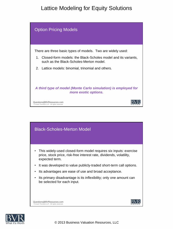
Option Pricing Models

There are three basic types of models. Two are widely used:

1. Closed-form models: the Black-Scholes model and its variants,

such as the Black-Scholes-Merton model.

2. Lattice models: binomial, trinomial and others.

A third type of model (Monte Carlo simulation) is employed for

more exotic options.


[email protected]

Black-Scholes-Merton Model

• This widely-used closed-form model requires six inputs: exercise

price, stock price, risk-free interest rate, dividends, volatility,

expected term.

• It was developed to value publicly-traded short-term call options.

• Its advantages are ease of use and broad acceptance.

• Its primary disadvantage is its inflexibility; only one amount can

be selected for each input.




[email protected]

Black-Scholes-Merton Example


[email protected]

Discussion of Inputs

You just saw traditional six inputs

common to all widely used option

pricing models.

The impact on option value of an

increase in each, while the others

are held constant, is summarized

here.




[email protected]

Lattice Models

• There are many variants of the lattice model; two of the most

common are the binomial and trinomial models.

• Unlike the closed-form models, lattice models visually display the

option valuation process.

• The term "lattice" derives from the appearance of the binomial

"tree" used to solve the option’s value.

• The valuation process is best illustrated by separating the model

into two separate trees, as shown in the following slides.


[email protected]

The "Underlying Asset Tree"

• As mentioned, the first step in valuing a call option is to estimate potential future prices of the underlying stock.

• The range of potential future values depends on three parameters:

1. Today’s stock price

2. The expected future volatility of the stock price

3. The term of the option

• In a binomial model, these factors are modeled in a 'lattice' (the underlying asset tree):

– It calculates the expected evolution of the underlying stock price at various future time periods leading up to the option expiry date.




[email protected]

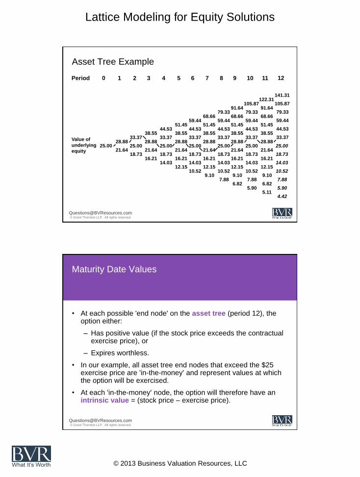
Asset Tree Example

Period 0 1 2 3 4 5 6 7 8 9 10 11 12

141.31 122.31

105.87 105.87 91.64 91.64

79.33 79.33 79.33 68.66 68.66 68.66

59.44 59.44 59.44 59.44 51.45 51.45 51.45 51.45

44.53 44.53 44.53 44.53 44.53 38.55 38.55 38.55 38.55 38.55

33.37 33.37 33.37 33.37 33.37 33.37 28.88 28.88 28.88 28.88 28.88 28.88

Value of

underlying

equity 25.00 25.00 25.00 25.00 25.00 25.00 25.00

21.64 21.64 21.64 21.64 21.64 21.64 18.73 18.73 18.73 18.73 18.73 18.73

16.21 16.21 16.21 16.21 16.21 14.03 14.03 14.03 14.03 14.03

12.15 12.15 12.15 12.15 10.52 10.52 10.52 10.52

9.10 9.10 9.10 7.88 7.88 7.88

6.82 6.82 5.90 5.90

5.11 4.42


[email protected]

Maturity Date Values

• At each possible 'end node' on the asset tree (period 12), the option either:

– Has positive value (if the stock price exceeds the contractual exercise price), or

– Expires worthless.

• In our example, all asset tree end nodes that exceed the $25 exercise price are 'in-the-money' and represent values at which the option will be exercised.

• At each 'in-the-money' node, the option will therefore have an intrinsic value = (stock price – exercise price).




[email protected]

The Option Solution Tree

• Once the 'in-the-money' end nodes are identified and valued, a second

'lattice' (the solution tree) is then employed.

• Unlike the asset tree, which shows the evolution in time from left-to-right,

the solution tree operates from right-to-left, performing two operations.

• Each end-value is probability-weighted and then discounted back one

period, i.e., the value in period 11 is calculated based on its two related

period 12 values.

• This weighting and discounting process is repeated in what is referred to

as a 'backward-solving' process until the period 0 (valuation date) is

reached.

• Note the consistency of the binomial result with the Black-Scholes value

calculated earlier.


[email protected]

Solution Tree Example

Period 0 1 2 3 4 5 6 7 8 9 10 11 12

116.31 97.38

81.00 80.87 66.83 66.71

54.58 54.45 54.33 43.98 43.85 43.73

34.81 34.68 34.56 34.44 26.95 26.76 26.63 26.51

20.36 20.04 19.78 19.66 19.53 14.98 14.54 14.11 13.73 13.61

10.74 10.23 9.69 9.10 8.49 8.37 7.52 7.00 6.42 5.77 4.98 3.94 Value of

Option 5.14 4.66 4.13 3.53 2.81 1.86 0.00 3.03 2.59 2.10 1.54 0.88 0.00

1.59 1.22 0.83 0.41 0.00 0.00 0.70 0.44 0.19 0.00 0.00

0.23 0.09 0.00 0.00 0.00 0.04 0.00 0.00 0.00

0.00 0.00 0.00 0.00 0.00 0.00 0.00

0.00 0.00 0.00 0.00 0.00

0.00 0.00 0.00

0.00




[email protected]

Consistency of the Binomial Result with the Black-

Scholes Value


[email protected]

Comparison of Models

• As the previous examples show, both the B-S-M and binomial models

produce results that are substantially similar.

– If the number of periods used in the binomial model is increased,

the binomial model’s value converges with the B-S-M if the same

inputs are used in each model.

• The advantage goes to the binomial model if flexibility of inputs is

important;

– i.e., the binomial model can accommodate assumptions that change

over time; the B-S-M cannot.




[email protected]

Types of Lattice Models

• Equity

• Debt/Interest rate

• Binomial, trinomial

• Single v. multiple risk resolution

• Lognormal vs. mean-reverting

The focus of this presentation will be on equity

solutions using lognormally distributed binomial

lattice models.


[email protected]

Lattice Models in Debt Valuations

• When debt has a call or put feature, the debt has a variable

rather than a contractual life as it can be called/put, and can

therefore terminate before maturity.

• The value of the call/put option is driven by the shape of the

yield curve and the terms of the embedded call/put feature.

• One model to value callable/putable debt is the Black-

Derman-Toy (BDT) model.

• The BDT model assumes that interest rates follow a

binomial process and uses current observed yields and

yield volatility to estimate future outcomes for the yields (by

means of a binomial tree of future interest rates).




[email protected]

Lattice Models in Valuations of Hybrid Securities

• Can be used to value convertible debt.

• Holder may convert to equity depending on stock

price.

• At each time interval, model compares

– Value of conversion

– Value of holding conversion option to next

period

• Optimal decision is selected


[email protected]

Lattice Models in Equity Valuations

• Can be used to value enterprises and business

segments.

• Can be used to allocate value between different

classes of equity in "cheap stock" valuations

performed for 409(A) tax purposes.

• Can be used to value stock options for financial

reporting purposes.

• Other uses?




[email protected]

Building a Lattice Model

Valuation of a Risky Business Opportunity

Market Risk Only

Pre-revenue stage

• Value of opportunity today: $1.0 million

• Annual volatility of opportunity: 50 percent

• Estimated time to commercialization: 6 months

• Cost of commercialization/product rollout: $0.8 million

• Risk-free rate: 3.0 percent

What is the value of this opportunity?


[email protected]

Mapping Opportunity onto the Black-Scholes Model

• Value of underlying asset = $1.0 million

• Strike Price = $0.8 million

• Time to expiry = 6 months

• Risk-free rate (annual) = 3.0 percent

• Volatility (annual) = 50 percent

• Value = $259,000




[email protected]

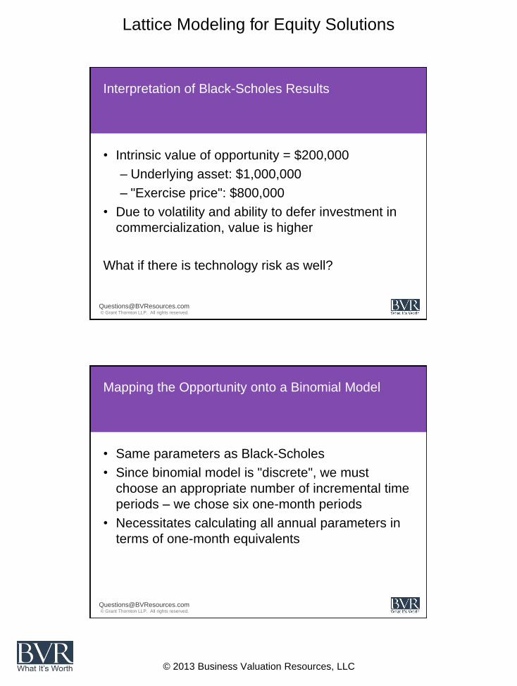
Interpretation of Black-Scholes Results

• Intrinsic value of opportunity = $200,000

– Underlying asset: $1,000,000

– "Exercise price": $800,000

• Due to volatility and ability to defer investment in

commercialization, value is higher

What if there is technology risk as well?


[email protected]

Mapping the Opportunity onto a Binomial Model

• Same parameters as Black-Scholes

• Since binomial model is "discrete", we must

choose an appropriate number of incremental time

periods – we chose six one-month periods

• Necessitates calculating all annual parameters in

terms of one-month equivalents




[email protected]

Calculation of Volatility

• Volatility varies with the square root of time

• Annual volatility = monthly volatility times square

root of 12 (12 monthly periods)

• Therefore, monthly volatility = annual volatility

divided by square root of 12

• 50%/(sq rt 12) = 14.43 percent per month


[email protected]

Calculation of Binomial "Jumps"

• Up movements (lognormal) are equal to the

exponential of the volatility

• Exp(0.1443) = 1.1553

• Down movements are the multiplicative inverse of

the up movements

• 1/1.1553 = 0.8656




[email protected]

Probabilities of Up and Down Jumps

• These are often referred to as "risk-neutral

probabilities"

• They are a function of risk-free rates and the

magnitude of up and down moves

• Formula: [exp(Rf) – down]/[up – down]

• In our case: [1.0025 – 0.8656]/[1.1553-0.8656] =

0.4725 is probability of an up move

• Down move = 1 – up = 0.5275


[email protected]

The Underlying Asset Value Tree

• Value today is $1.0 million

• Value in one month, if "market" is up, is $1,155,300 ($1.0

million x 1.1553) and has a 47.25 percent "probability"

• Value in one month, if "market" is down, is $865,600 ($1.0

million x 0.8656) and has a 52.75 percent "probability"

• Therefore, value in six months may range from $2,377,000

(six consecutive up moves) to $421,000 (six consecutive

down moves)

What is the probability of six consecutive up moves?




[email protected]

Annual volatility 50% Rf/year 3.00%

Per period 0.1443 Rf/period 1.0025

Up movement 1.1553 p 0.4726

Down movement 0.8656 1-p 0.5274

Period 0 1 2 3 4 5 6

Value of opportunity 1,000 1,155 1,335 1,542 1,781 2,058 2,377

866 1,000 1,155 1,335 1,542 1,781

749 866 1,000 1,155 1,335

649 749 866 1,000

561 649 749

486 561

421

The Underlying Asset


[email protected]

Our Rollout Decision

• We will commercialize only if value exceeds $0.8

million cost

• Four of our seven outcomes are "in-the-money"

and provide us with positive values net of exercise

cost

• Bringing these values back to the present by

applying risk-neutral probabilities and discounting

at the monthly risk-free rate, we get a value of

$260,000




[email protected]

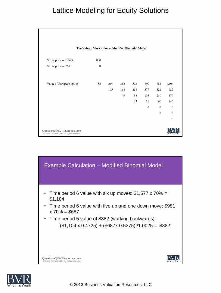
Strike price 800

Value of current equity 260 384 547 748 985 1,260 1,577

150 240 369 539 744 981

71 126 218 357 535

21 44 94 200

0 0 0

0 0

0

Value of the Opportunity


[email protected]

Example Calculation – Binomial Model

• Time period 6 value with six up moves: $1,000 x

(1.1553)6 = $2,377 – 800 exercise cost = $1,577

• Time period 6 value with five up and one down

move: $1,000 x (1.1553)5 x 0.8656 = $1,781 – 800

= $981

• Time period 5 value of $1,260 (working

backwards):

[($1,577 x 0.4725) + ($981 x 0.5275)]/1.0025 =

$1,260




[email protected]

Modified Binomial Model

• Why did we go through the effort on the binomial model if

the Black-Scholes model gives us the same result?

– Because the binomial model lends itself to customization

• A simple example – we add a second risk and a second

investment decision:

– Technology risk: 30 percent chance technology fails at

the end of six months

– Cost of R&D efforts to prove out technology: $100,000,

which must be invested today

• The value ($82,000) is calculated directly by this modified

binomial model


[email protected]

Expanding the Lattice Model

Multiple Risks, Multiple Investment Decisions

• Value of opportunity if technology is successful: $1.0 million

• Annual volatility of opportunity – market risk only: 50

percent

• Chance of achieving technological success: 70 percent

• Cost of R&D to prove technology: $0.1 million

• Estimated time to completion of R&D: 6 months

• Cost of commercialization/product rollout: $0.8 million




[email protected]


[email protected]

Example Calculation – Modified Binomial Model

• Time period 6 value with six up moves: $1,577 x 70% =

$1,104

• Time period 6 value with five up and one down move: $981

x 70% = $687

• Time period 5 value of $882 (working backwards):

[($1,104 x 0.4725) + ($687x 0.5275)]/1.0025 = $882




[email protected]

Lattice Models in Equity Allocation

• Three methodologies for allocating value between

different classes of equity.

– Current value method

– Option pricing method

• Black-Scholes

• Lattice

– Probability-weighted expected return method


[email protected]

When should a lattice model be used?

Can be helpful in allocations when:

• Allocation changes completely above a certain equity value (e.g., auto-

conversion upon IPO).

• Classes of equity receive different payouts based upon the

achievement of certain metrics and/or liquidation value.

– A class of preferred stock may be pari passu with the other

preferred at certain exit values, but first in order of preference at

other exit values to guarantee them a certain return.

– Management may receive a "carveout" – a certain percentage of the

exit value when exit values fall within a certain range.




[email protected]

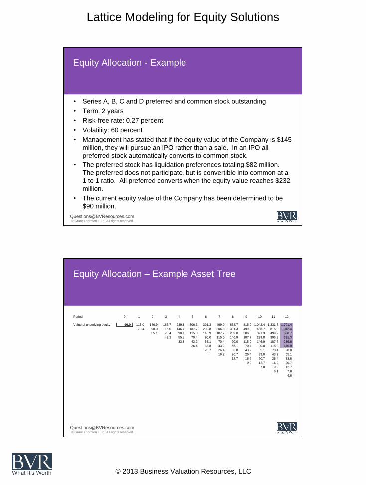
Equity Allocation - Example

• Series A, B, C and D preferred and common stock outstanding

• Term: 2 years

• Risk-free rate: 0.27 percent

• Volatility: 60 percent

• Management has stated that if the equity value of the Company is $145

million, they will pursue an IPO rather than a sale. In an IPO all

preferred stock automatically converts to common stock.

• The preferred stock has liquidation preferences totaling $82 million.

The preferred does not participate, but is convertible into common at a

1 to 1 ratio. All preferred converts when the equity value reaches $232

million.

• The current equity value of the Company has been determined to be

$90 million.


[email protected]

Equity Allocation – Example Asset Tree

Period 0 1 2 3 4 5 6 7 8 9 10 11 12

Value of underlying equity 90.0 115.0 146.9 187.7 239.8 306.3 391.3 499.9 638.7 815.9 1,042.4 1,331.7 1,701.4

70.4 90.0 115.0 146.9 187.7 239.8 306.3 391.3 499.9 638.7 815.9 1,042.4

55.1 70.4 90.0 115.0 146.9 187.7 239.8 306.3 391.3 499.9 638.7

43.2 55.1 70.4 90.0 115.0 146.9 187.7 239.8 306.3 391.3

33.8 43.2 55.1 70.4 90.0 115.0 146.9 187.7 239.8

26.4 33.8 43.2 55.1 70.4 90.0 115.0 146.9

20.7 26.4 33.8 43.2 55.1 70.4 90.0

16.2 20.7 26.4 33.8 43.2 55.1

12.7 16.2 20.7 26.4 33.8

9.9 12.7 16.2 20.7

7.8 9.9 12.7

6.1 7.8

4.8




[email protected]

Equity Allocation - Example

• The preferred would not fully convert to common stock until $232 million

under a sale.

• Because management will pursue an IPO at lower values, there are

nodes where preferred stock's optimal outcome would be to receive its

liquidation preference, but it does not.

• This results in a higher value to the common stock.

• For the highlighted (IPO) nodes, common receives the asset value

times their pro rata interest. (12.1 percent in this example)

• For nodes below that, common's value is determined based on the

equity breakpoints, which consider preferred liquidation preferences

and conversion rights.


[email protected]

Equity Allocation – Example Common Stock Tree

Period 0 1 2 3 4 5 6 7 8 9 10 11 12

Value of common stock 7.09 10.3 14.7 20.4 27.5 36.3 47.0 60.3 77.1 98.5 125.8 160.7 205.3

4.5 6.9 10.3 14.8 20.6 27.9 36.6 47.2 60.3 77.1 98.5 125.8

2.7 4.3 6.7 10.2 14.9 21.0 28.3 37.0 47.2 60.3 77.1

1.4 2.4 4.0 6.5 10.2 15.2 21.6 28.9 37.0 47.2

0.6 1.1 2.0 3.6 6.2 10.2 15.9 22.6 28.9

0.2 0.4 0.8 1.6 3.1 5.8 10.5 17.7

0.0 0.1 0.2 0.4 0.9 2.1 4.9

0.0 0.0 0.0 0.0 0.0 0.0

0.0 0.0 0.0 0.0 0.0

0.0 0.0 0.0 0.0

0.0 0.0 0.0

0.0 0.0

0.0




[email protected]

Lattice Models to Value Stock Options

• ASC Topic 718 requires entities to use

– Fair-value-based measurement method

• To estimate value of employee awards

• Entities required to apply requirements of fair-

value-based measurement method in determining

award value


[email protected]

Explicitly Excluded Characteristics

• Service conditions

• Performance conditions that affect vesting or

exercisability

• Vesting period restrictions

• Reload features

• Certain contingent features (e.g., clawbacks)




[email protected]

Hull-White Lattice

• Lattice model to value employee stock options

• Accounts for possibility of early exercise and termination

• Example:

– Stock price: $100

– Strike price: $100

– Volatility: 35 percent

– Risk-free rate: 5 percent

– Term: 6 years

– Vesting period: 3 years

– Early exercise assumed when stock price is twice the strike price.

– The annual probability the employee will terminate is 3.0 percent.


[email protected]

Hull-White Example

• Used a 24-period lattice model (4 periods per year)

• The up movement is calculated at 1.1912 = EXP(0.35/SQRT(4))

• The down movement is calculated at 0.8395 = (1/1.1912)

• The up probability is calculated at 49.12% = (EXP(0.05)-

0.8395)/(1.1912-0.8395)

• The down probability is calculated at 50.88% = 1-0.4912

• First step is to prepare an asset tree for underlying stock price




[email protected]

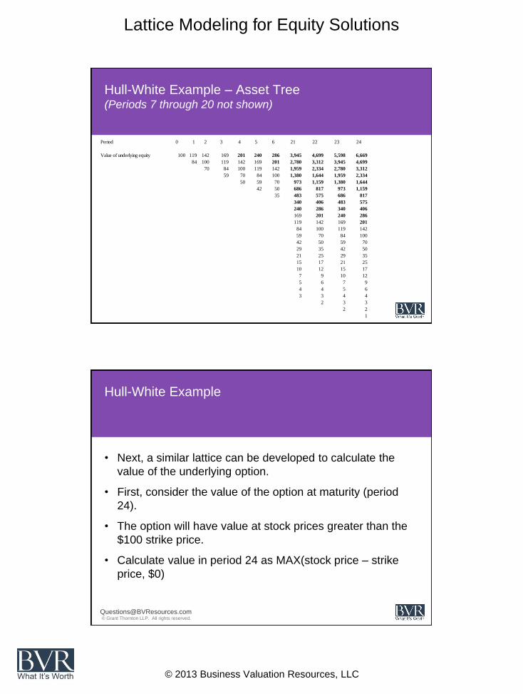
Hull-White Example – Asset Tree (Periods 7 through 20 not shown)

Period 0 1 2 3 4 5 6 21 22 23 24

Value of underlying equity 100 119 142 169 201 240 286 3,945 4,699 5,598 6,669

84 100 119 142 169 201 2,780 3,312 3,945 4,699

70 84 100 119 142 1,959 2,334 2,780 3,312

59 70 84 100 1,380 1,644 1,959 2,334

50 59 70 973 1,159 1,380 1,644

42 50 686 817 973 1,159

35 483 575 686 817

340 406 483 575

240 286 340 406

169 201 240 286

119 142 169 201

84 100 119 142

59 70 84 100

42 50 59 70

29 35 42 50

21 25 29 35

15 17 21 25

10 12 15 17

7 9 10 12

5 6 7 9

4 4 5 6

3 3 4 4

2 3 3

2 2

1


[email protected]

Hull-White Example

• Next, a similar lattice can be developed to calculate the

value of the underlying option.

• First, consider the value of the option at maturity (period

24).

• The option will have value at stock prices greater than the

$100 strike price.

• Calculate value in period 24 as MAX(stock price – strike

price, $0)




[email protected]

Hull-White Example

• Then, consider the value of the option in nodes prior to maturity (1-23).

• Early exercise and termination will be factors in these nodes.

– IF(stock price > 2x strike after vesting, stock price – strike),

accounts for voluntary early exercise (also referred to as suboptimal

exercise and the 2x multiple is referred to as the S.O.E.F.)

– IF(stock price < 2x strike)

• (1-.0075) x [(0.4912 x $6,569) + (0.5088 x $4,599)]/1.012 hold

• + 0.0075 x MAX(stock price – strike, $0) exercise if terminated

(also referred to as post-vesting termination factor)


[email protected]

Hull-White Example – Solution Tree

Period 0 1 2 3 4 5 6 21 22 23 24

Value of option 35.65 48 64 85 111 144 186 3,845 4,599 5,498 6,569

25 34 47 63 83 110 2,680 3,212 3,845 4,599

17 24 33 45 61 1,859 2,234 2,680 3,212

11 16 23 32 1,280 1,544 1,859 2,234

7 10 15 873 1,059 1,280 1,544

4 6 586 717 873 1,059

2 383 475 586 717

240 306 383 475

140 186 240 306

71 101 140 186

26 44 70 101

5 10 20 42

0 0 0 0

0 0 0 0

0 0 0 0

0 0 0 0

0 0 0 0

0 0 0 0

0 0 0 0

0 0 0 0

0 0 0 0

0 0 0 0

0 0 0

0 0

0




[email protected]

Lattice Models in Valuation/Real Options

• Lattice models can be used to capture need for

future financing and possible future dilution

• Discussed in new AICPA Accounting & Valuation

Guide Valuation of Privately-Held-Company Equity

Securities Issued as Compensation


[email protected]

Using a Lattice Model to Capture Future Milestones

• Can adjust a lattice model to account for future

rounds of financing prior to a liquidity event.

• This is modeled as a sequence of options or

"compound option"

• Can address spikes in value due to success/failure

of financing rounds and technological/market risk

resolution




[email protected]

Using a Lattice Model to Capture Future Milestones - Example

• Value of company (ignoring need for future

financing): $2.0 million

• Current capital structure is Series A preferred and

common stock.

• Volatility: 80 percent

• Risk-free rate: 3 percent

• Company requires financing of $800,000 in one

year (Series B) and $1.5 million in three years

(Series C) to achieve an exit.


[email protected]

Future Milestones - Asset Tree

Period 0 1 2 3 4 5 6 7 8 9 10 11 12

Value of opportunity 2,000 2,984 4,451 6,640 9,906 14,778 22,046 32,889 49,065 73,196 109,196 162,902 243,021

1,341 2,000 2,984 4,451 6,640 9,906 14,778 22,046 32,889 49,065 73,196 109,196

899 1,341 2,000 2,984 4,451 6,640 9,906 14,778 22,046 32,889 49,065

602 899 1,341 2,000 2,984 4,451 6,640 9,906 14,778 22,046

404 602 899 1,341 2,000 2,984 4,451 6,640 9,906

271 404 602 899 1,341 2,000 2,984 4,451

181 271 404 602 899 1,341 2,000

122 181 271 404 602 899

82 122 181 271 404

55 82 122 181

37 55 82

25 37

16




[email protected]

Future Milestones – First and Second Option

• Determine when the second option (opportunity to

invest $1.5 million in Series C) would be exercised.

– This would happen at equity values above $1.5

million in period 12.

• Determine when the first option (opportunity to

invest $0.8 million in Series B) would be exercised.

– This would happen at equity values above $0.8

million in period 4.


[email protected]

Future Milestones – Tree with First and Second Option

Value of current equity 693.31 1,351 2,548 4,594 7,754 13,369 20,612 31,445 47,609 71,730 107,719 161,413 241,521

244 535 1,156 2,453 5,312 8,496 13,333 20,591 31,423 47,587 71,708 107,696

45 109 268 1,861 3,162 5,237 8,450 13,311 20,569 31,401 47,565

0 0 530 978 1,758 3,066 5,174 8,428 13,289 20,546

0 111 225 448 869 1,637 2,973 5,151 8,406

15 33 73 160 345 728 1,495 2,951

2 6 14 34 83 204 500

0 0 0 0 0 0

0 0 0 0 0

0 0 0 0

0 0 0

0 0

0




[email protected]

Future Milestones – Accounting for Dilution

• At valuation date, only Series A and common outstanding.

• At period 12, the Series C has been removed, but the

dilution from Series B still exists.

• How can we determine the dilution from the Series B

financing that exists in the period 12 nodes?

– Determine the extent to which the Series B investors

dilute the holdings of the Series A and common at the

end of year one (assuming a Series B financing occurs).

– Determine how this financing affects the year three exit

values.

– Remove the Series B dilution from the exit date values.


[email protected]

Summary

• Review of option valuation fundamentals

• Types of lattice models

• How to build a simple equity lattice model

• Equity solutions using lattice models

– Equity valuation

– Equity allocation

– Options on equity

• Advanced applications




[email protected]

Questions?

Documents

Lattice Modeling for Equity Solutions David C. Dufendach, CPA/ABV