Embed Size (px)
Citation preview
Lattice-Boltzmann Simulations of ParticleSuspensions in Sheared Flow
Eric Lorenz, Alfons G. Hoekstra
Section Computational Science, Faculty of ScienceUniversity of Amsterdam
28/09/2007
Outline
• Lattice-Boltzmann Method (LBM)• Suspension Modeling with LBM• Lees-Edwards Boundary Conditions (LEBC) for LBM Suspensions• Rheology of Suspensions (Validation of LEBC)• Some Cluster Properties
1
Lattice-Boltzmann Method (LBM)
2
LBM’s Predecessor: Lattice-Gas Automaton
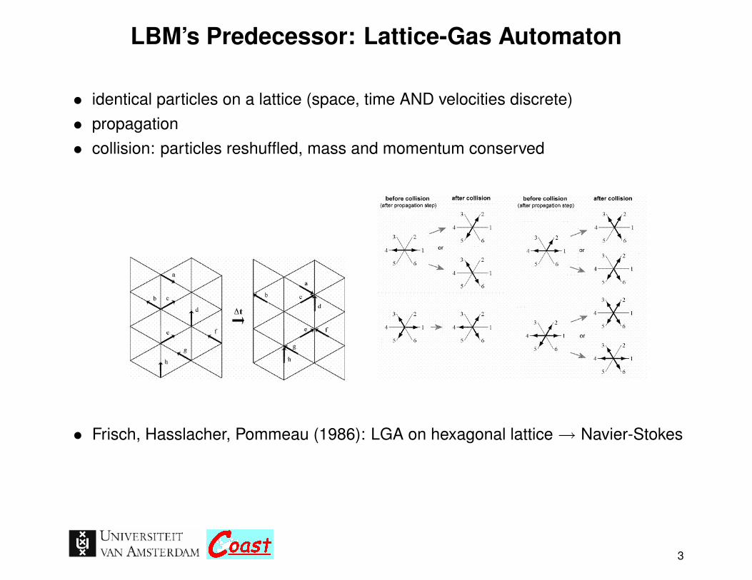
• identical particles on a lattice (space, time AND velocities discrete)• propagation• collision: particles reshuffled, mass and momentum conserved
• Frisch, Hasslacher, Pommeau (1986): LGA on hexagonal lattice→ Navier-Stokes
3
Lattice-Boltzmann method
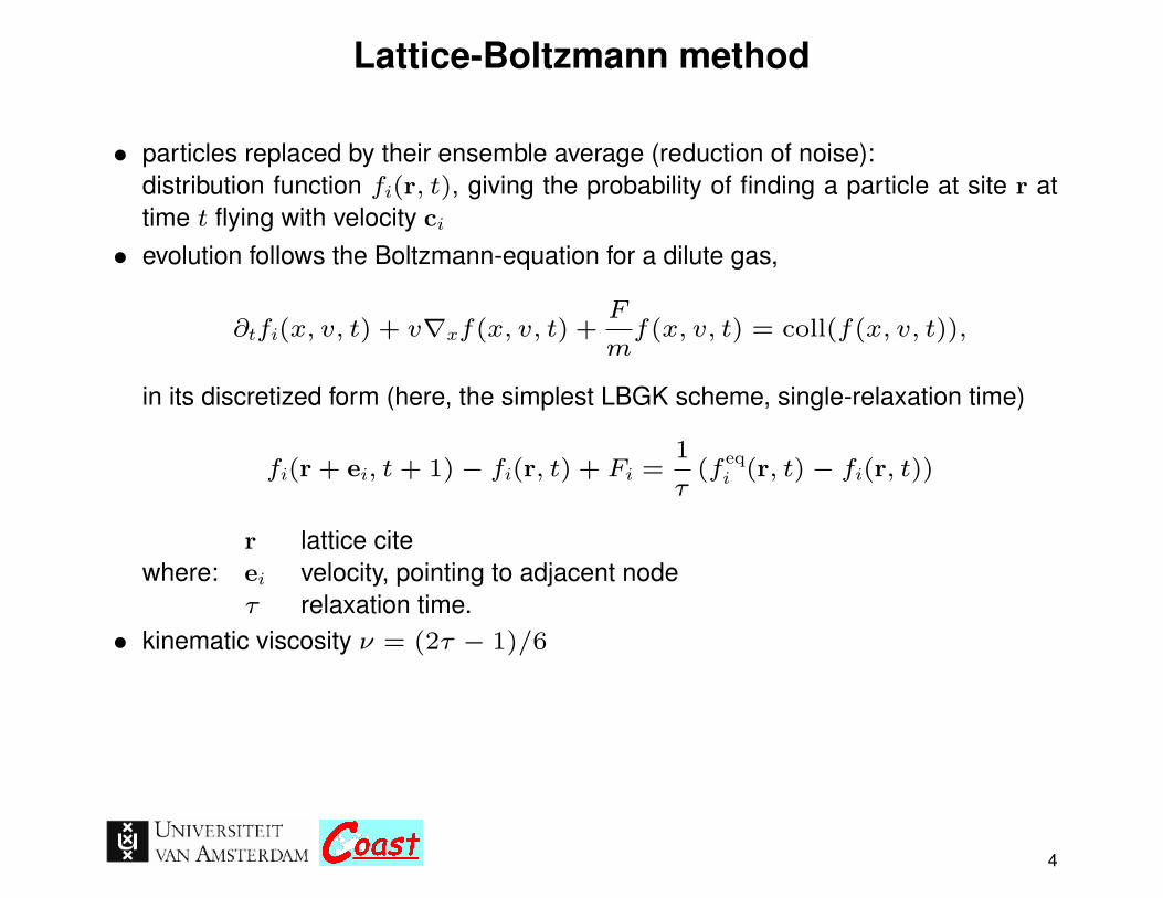
• particles replaced by their ensemble average (reduction of noise):distribution function fi(r, t), giving the probability of finding a particle at site r attime t flying with velocity ci
• evolution follows the Boltzmann-equation for a dilute gas,
∂tfi(x, v, t) + v∇xf(x, v, t) +F
mf(x, v, t) = coll(f(x, v, t)),
in its discretized form (here, the simplest LBGK scheme, single-relaxation time)
fi(r + ei, t+ 1)− fi(r, t) + Fi =1
τ(f
eqi (r, t)− fi(r, t))
where:r lattice citeei velocity, pointing to adjacent nodeτ relaxation time.
• kinematic viscosity ν = (2τ − 1)/6
4
Lattice-Boltzmann method
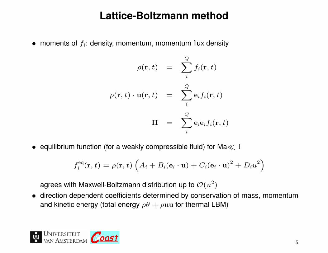
• moments of fi: density, momentum, momentum flux density
ρ(r, t) =
QXi
fi(r, t)
ρ(r, t) · u(r, t) =
QXi
eifi(r, t)
Π =
QXi
eieifi(r, t)
• equilibrium function (for a weakly compressible fluid) for Ma� 1
feqi (r, t) = ρ(r, t)
“Ai + Bi(ei · u) + Ci(ei · u)
2+Diu
2”
agrees with Maxwell-Boltzmann distribution up to O(u2)
• direction dependent coefficients determined by conservation of mass, momentumand kinetic energy (total energy ρθ + ρuu for thermal LBM)
5
D2Q9 LBM
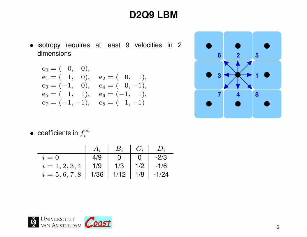
• isotropy requires at least 9 velocities in 2dimensions
e0 = ( 0, 0),e1 = ( 1, 0), e2 = ( 0, 1),e3 = (−1, 0), e4 = ( 0,−1),e5 = ( 1, 1), e6 = (−1, 1),e7 = (−1,−1), e8 = ( 1,−1)
847
3
6 2 5
1
• coefficients in f eqi
Ai Bi Ci Di
i = 0 4/9 0 0 -2/3i = 1, 2, 3, 4 1/9 1/3 1/2 -1/6i = 5, 6, 7, 8 1/36 1/12 1/8 -1/24
6

Modelling of Suspensions with LBM
7

The ALD method for suspended particles
(Aidun, Lu, Ding, 2003)
• particles mapped to lattice→ broken links
• virtual fluid inside shell• arbitrary surfaces possible
• solid-fluid interaction: (bounce-back at the links with moving wall)
fi(x, t+ 1) =
f−i(x, t
+) + 2ρBiub · ei if BL
fi(x + e−i, t+) else
• momentum exchange, force, torque:
δpi = 2ei[fi(x, t+ 1)− ρBiub · ei]
Fi(x, t0 +1/2) = δpi/∆t, Ti(x, t0 +1/2) = (x−X(t0)×Fi(x, t0 +1/2))
8
Lees-Edwards Boundary Conditions for LBMSuspensions
9

Lees-Edwards Boundaries for Suspensions
wu
f5
Procedure for boundary-crossing densities:- Mapping to off-grid copy (distribute f over destination nodes according to sub-gridshift ratio):
f5(x, 1) = (1−mod1[ut]) · f5(x+ int[x− ut], ymax)
+ mod1[ut] · f5(x+ int[x− ut− 1], ymax)
10
Lees-Edwards Boundaries for Suspensions
wu
f5
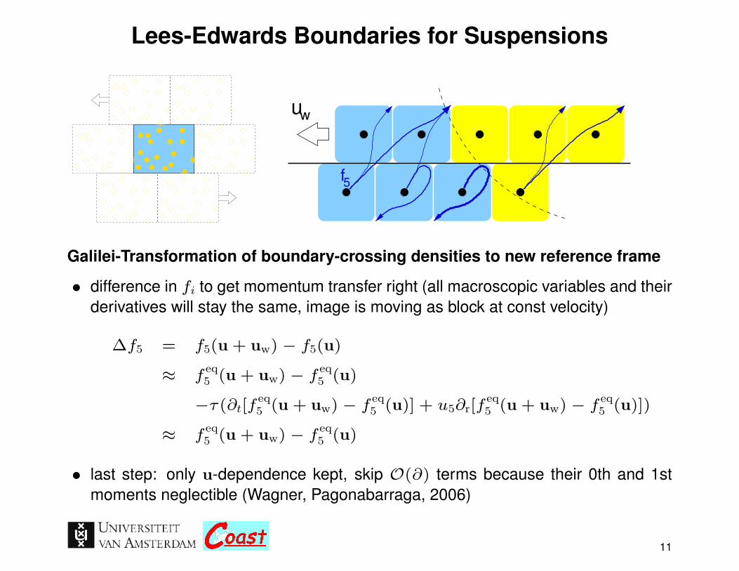
Galilei-Transformation of boundary-crossing densities to new reference frame
• difference in fi to get momentum transfer right (all macroscopic variables and theirderivatives will stay the same, image is moving as block at const velocity)
∆f5 = f5(u + uw)− f5(u)
≈ feq5 (u + uw)− f eq
5 (u)
−τ(∂t[feq5 (u + uw)− f eq
5 (u)] + u5∂r[feq5 (u + uw)− f eq
5 (u)])
≈ feq5 (u + uw)− f eq
5 (u)
• last step: only u-dependence kept, skip O(∂) terms because their 0th and 1stmoments neglectible (Wagner, Pagonabarraga, 2006)
11

Lees-Edwards Boundaries for Suspensions
wu
f5
Sub-grid Boundary Reflection (according to sub-grid shift ratio):
• modification of distribution step to allow fluid-solid interaction
fi(x, t+ 1) = (1−mod1[uwt]) ·fi(x− int[x− uwt] + ei, t
+)
f−i(x, t+)− ρBiub · ei if BL
+ mod1[uwt] ·fi(x− int[x− uwt+ 1] + ei, t
+)
f−i(x, t+)− ρBiub · ei if BL
12
Rheology of Suspensions
13

Apparent Viscosity, Dependence on Concentration φ
• for a dilute dispersed suspension (Einstein, 1906): νapp = νf(1 + 2.5φ)
assumptions: no hydrodynamical interaction (∼ φ2) , Brownian motion insignificant• semi-empirical Krieger-Dougherty relation:
νapp = νf
„1−
φ
φmax
«−[η]φmax
(1)
• simulation results for R = 8, Re = 0.001
0
1
2
3
4
5
6
7
0 0.1 0.2 0.3 0.4 0.5
ν app
/νf
φ
Krieger-DoughertyEinstein
Re=0.001
14

App. Viscosity νapp as a Function of Shear Rate γ
• generic behaviour
νlo
g
I II III IV V
log γ
φ
– I - Newtonian plateau: Brownian motion dominates– II - shear-thinning: increasing shear decreases disorder of particle structure– III - Newtonian plateau: particles strongly orientated– IV - shear-thickening: local structures, broken by shear, momentum transfer via
particles dominates– V - unknown: some experimental results show repeated shear-thinning
15

Shear-Thickening
• Rp = 8, Lx,y = 259 ≈ 16 · 2Rp, φ = 0.40, νf = 0.0125, uw < 0.0864
Lees-Edwards vs. planar Couette scheme
0.9
1
1.1
1.2
1.3
1.4
1.5
1.6
1.7
1.8
1.9
-2.5 -2 -1.5 -1 -0.5 0 0.5
ν eff/
(1-φ
s/φ m
ax)-[
η]φ m
ax
log(Reshear,p)
φ=0.40 (Kromkamp+)φ=0.40 (Lees-Edwards)
φ=0.40 Couette
0
20
40
60
80
100
-2.5 -2 -1.5 -1 -0.5 0
τ s,f/
τ T
log(Reshear,p)
solidfluid
0.8
0.85
0.9
0.95
1
1.05
1.1
0 50 100 150 200 250
φ(y)
/<φ>
y
Couette, φ=0.40, Re=1.8Lees-Edwards, φ=0.40, Re=1.8
-1
-0.5
0
0.5
1
0 50 100 150 200 250
u x(y
)/uw
y
Couette, φ=0.40, Re=1.8Lees-Edwards, φ=0.40, Re=1.8
• clear: Couette scheme suffers from wall effects at higher shear rates γ– wall induces different particle structures→ depletion zone→ wall slip→ lower
apparent viscosity
16
Particle Clusters
17

Emerging Particle ClustersSnapshot of a sheared suspension
Rpart = 3.75, Reshear,part ≈ 0.1, φ = 0.431, red∼high pressure
18
Cluster Properties
30
20
10
0
10
20
30
25 20 15 10 5 0 5 10 15 20 25
angle distribution of particle in a cluster
0.0001
0.001
0.01
0.1
1
10
100
1 10 100
n(m
)
m
Re=1.0Re=0.1
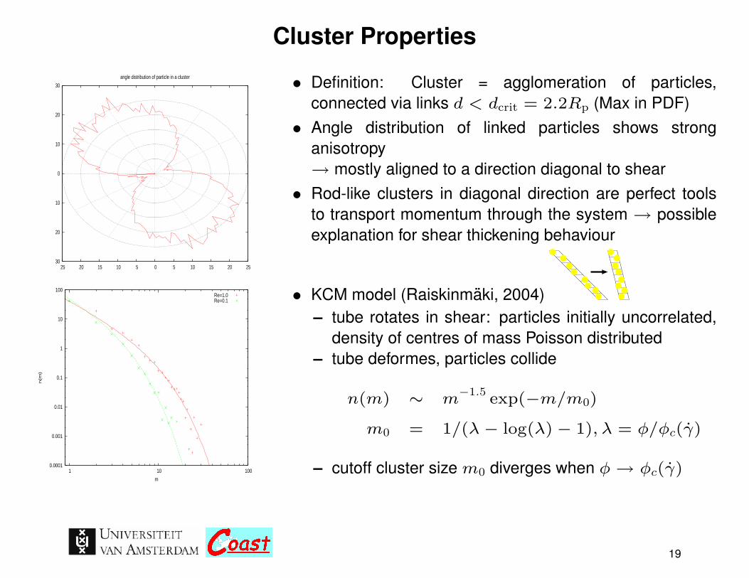
• Definition: Cluster = agglomeration of particles,connected via links d < dcrit = 2.2Rp (Max in PDF)
• Angle distribution of linked particles shows stronganisotropy→ mostly aligned to a direction diagonal to shear
• Rod-like clusters in diagonal direction are perfect toolsto transport momentum through the system→ possibleexplanation for shear thickening behaviour
• KCM model (Raiskinmaki, 2004)– tube rotates in shear: particles initially uncorrelated,
density of centres of mass Poisson distributed– tube deformes, particles collide
n(m) ∼ m−1.5
exp(−m/m0)
m0 = 1/(λ− log(λ)− 1), λ = φ/φc(γ)
– cutoff cluster size m0 diverges when φ→ φc(γ)
19
Outlook
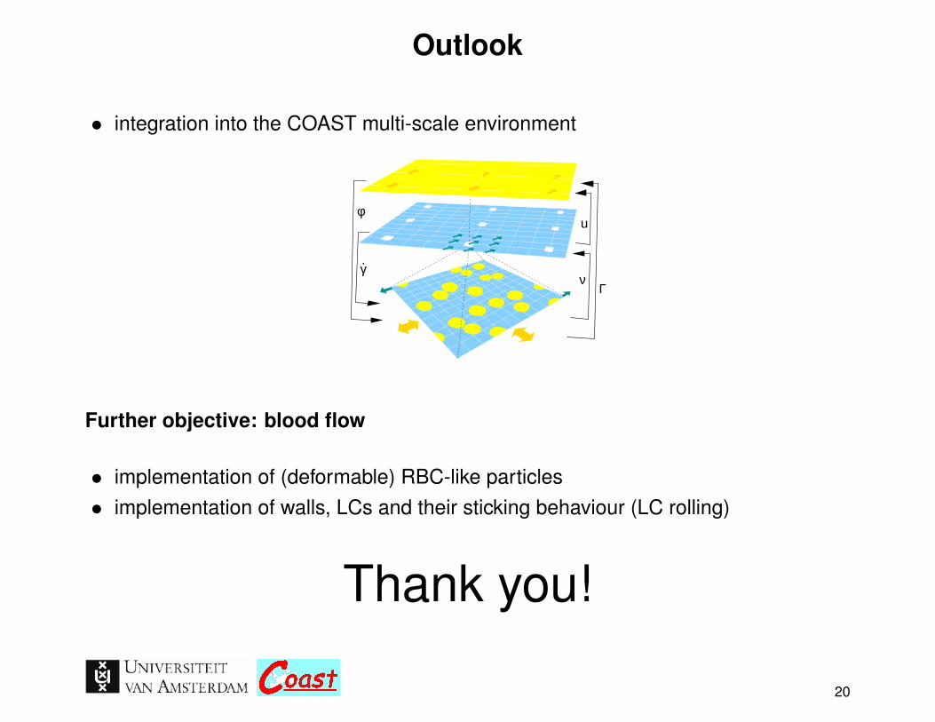
• integration into the COAST multi-scale environment
φ
γ.
u
Γν
Further objective: blood flow
• implementation of (deformable) RBC-like particles• implementation of walls, LCs and their sticking behaviour (LC rolling)
Thank you!
20


![From Lattice Boltzmann Method to Lattice Boltzmann Flux … · From Lattice Boltzmann Method to Lattice Boltzmann Flux Solver Yan Wang 1, ... flows [8,13–15], compressible flows](https://img.pdfslide.us/doc/110x75/5cadf91b88c9938f4d8c0cd6/from-lattice-boltzmann-method-to-lattice-boltzmann-flux-from-lattice-boltzmann.jpg)