Embed Size (px)
Citation preview

Lateral-torsional buckling analysis of steel frames with corrugated webs A case study of tapered I-beams with trapezoidally corrugated webs Master’s Thesis in the Master’s programme Structural Engineering and Building Performance Design
ANNA KAROLINA SABAT Department of Civil and Environmental Engineering Division of Structural Engineering Steel and Timber Structures CHALMERS UNIVERSITY OF TECHNOLOGY Göteborg, Sweden 2009 Master’s Thesis 2009: 108


MASTER’S THESIS 2009: 108
Lateral-torsional buckling analysis of steel frames with corrugated webs
A case study of tapered I-beams with trapezoidally corrugated webs
Master’s Thesis in the International Master’s programme Structural Engineering and Building Performance Design
ANNA KAROLINA SABAT
Department of Civil and Environmental Engineering Division of Structural Engineering
Steel and Timber Structures CHALMERS UNIVERSITY OF TECHNOLOGY
Göteborg, Sweden 2009

Lateral-torsional buckling analysis of steel frames with trapezoidally corrugated webs A case study of tapered I-beams with trapezoidally corrugated webs Master’s Thesis in the International Master’s programme Structural Engineering and Building Performance Design ANNA KAROLINA SABAT
© ANNA KAROLINA SABAT, 2009
Master’s Thesis 2009: 108 Department of Civil and Environmental Engineering Division of Structural Engineering Steel and Timber Structures Chalmers University of Technology SE-412 96 Göteborg Sweden Telephone: + 46 (0)31-772 1000 Cover: Finite Element model showing lateral-torsional buckling of the analyzed frame with corrugated webs. Chalmers Reproservice / Department of Civil and Environmental Engineering Göteborg, Sweden 2009

I
Lateral-torsional buckling analysis of steel frames with trapezoidally corrugated webs A case study of tapered I-beams with trapezoidally corrugated webs Master’s Thesis in the International Master’s programme Structural Engineering and Building Performance Design ANNA KAROLINA SABAT
Department of Civil and Environmental Engineering Division of Structural Engineering Steel and Timber Structures Chalmers University of Technology
ABSTRACT
The focus of this Master’s thesis project has been on a stability problem in steel structures. The problem of lateral-torsional buckling of steel frames, consisted of tapered members with plane and corrugated webs, has been investigated.
A literature review has been undertaken focusing on lateral-torsional buckling analysis of prismatic and non-prismatic beams of I-profiles with corrugated webs. The most recent available calculation models have been investigated and discussed. This Master’s thesis project has also investigated the stability problem of columns in compression as well as simply supported beams under uniform bending. Load-displacement response has been investigated by performing several finite element analyses in ABAQUS. The obtained results have been compared to hand calculations based on Eurocode3 and the Polish Code PN-90/B-00320. In addition, parametric studies have been conducted using available calculation models for obtaining the elastic critical moment for I-beams with corrugated webs. Finally, the comparison between buckling behaviour of the frames with plane webs and the frames with corrugated webs has been made. In order to make such comparison several linear and non-linear finite element analyses have been carried out using the computer program ABAQUS.
The analyses have given the general result that the frame with corrugated webs and the frame with plane webs with vertical stiffeners have similar lateral-torsional buckling resistance. However, the behaviour of the frames differs to some extent. The results from the case study have shown that the out-of-plane deflection for the frame with plane webs has been higher than for the frame with corrugated webs. Further on, it has been found that, for the analysed frame geometry, the distance between the purlins does not affect the buckling capacity of analysed frames. However, it is important to keep in mind that all analyses have been performed only for one type of frame geometry and one load combination. In addition, one value of initial imperfections has been applied and one material type has been taken into consideration. That is why further investigation should be carried out for various frame geometries, loads combinations and initial imperfections.
Key words: Lateral-torsional buckling, Stability problem, Steel frames, Trapezoidally corrugated webs, Tapered Beams, Finite Element Analysis,

II
Analiza problemu zwichrzenia na przykladzie ram stalowych zbudowanych z profili o zmiennym przekroju oraz o srodniku z blachy falistej Praca Magisterska, Katedra Konstrukcji Stalowych ANNA KAROLINA SABAT Wydzial Inzynierii Ladowej i Srodowiska Budownictwo Konstrucjie Stalowe Politechnika Gdanska
STRESZCZENIE
Celem ninejszej Pracy Magisterskiej jest analiza problemu stabilnosci konstrukcji stalowych. Zagadnienie zwichrzenia stalowych ram zlozonych z elementow o zmiennym przekroju oraz o srodnikach z blachy trapzowej i plaskiej zostalo przeanalizowane.
Zostal rowniez przeprowadzony przeglad literatury dotyczacej zwichrzenia zarowno profili I o zmiennym przekroju jak rowniez profili I o srodnikach z blachy trapezowej. W tej Pracy Magisterskiej przeanalizowano rowniez problem stabilnosci osiowo sciskanych slupow oraz wolnopodpartych belek rownomiernie zginanych. Wykresy sily do przemieszczenia zostaly przeanalizowane przez przeprowadzenie serii Analiz wykorzystujacych metode elementow skonczonych przy uzyciu programu ABAQUS. Otrzymane wyniki zostaly porownane z recznymi obliczeniami przeprowadzonymi na podstawie Eurokodu3 oraz Polskeij Normy PN-90/B00320. Co wiecej, najnowsze dostepne procedury pozwalajace na obliczenie elastycznego momentu krytycznego dla profili I o srodniku z blachy trapezowej zostaly przedstawione. Ostatecznie, porownany zostal sposob wyboczenia ramy stalowej z plaskimi srodnikami oraz ram stalowej ze srodnikami z blachy trapezowej. Do tego celu seria liniowych oraz nieliniowych analiz wykorzystujacych Matode Elementow Skoczonych zostala przeprowadzona w programie ABAQUS.
Ogolnie zaobserwowano, ze zarowno rama z plaskimi srodnikami jak i rama ze srodnikami z blachy trapezowej zachowuja sie z sposob podobny pod zwgledem stabilnosci. Mimo to, do pewnego stopnia ich zachowanie sie rozni. Zauazono ze ramy z plaskimi srodnikami doznaja wiekszych odksztalcen z plaszczyzny dzialania sily niz ramy ze srodnikamia z balchy trapezowej. Idac dalej, stwierdzono, ze dla badanej ramy rozstaw platew nie odgrywa wiekszego znaczenia na stabilosc calej konstrukcji. Nalezy jednak pamietac, ze w przedstawionej analizi tylko jedna geometria ramy i jedna kombinacja obciazej zostala uwzgledniona. Co wiecej, zastosowano jedna wartosc imperfekcji oraz jeden gatunek stali. Dlatego tez, dalsze badania biarace pod uwage rozne wymiary ram, kombinacje obciazen i imperfekcjie powinny byc przeprowadzone.
Slowa kluczowe: Zwichrzenie, hale, ramy, problem stabilnosci, wyboczenie, srodnik z blachy trapezowej, przekroje o zmiennym przekroju, metoda elementow skonczonych,

Contents ABSTRACT I
CONTENTS I
PREFACE III
NOTATIONS IV
1 INTRODUCTION 1
1.1 Problem definition 1
1.2 Aim of the Master’s Project 2
1.3 Method 2
1.4 Scope and limitations 3
1.5 Outline of the Thesis 3
2 LITERATURE REVIEW 4
2.1 Lateral-torsional buckling behaviour of I-beams with corrugated webs 4
2.2 Lateral-torsional buckling behaviour of I-beams with tapered webs 8
2.3 Equivalent moment factor - different load and support conditions 10
2.4 Conclusions 12
3 STABILITY PROBLEM IN GENERAL 14
3.1 Case study of columns in compression 15 3.1.1 Hand calculations of design buckling resistance 15 3.1.2 Finite Element Analysis of design buckling resistance 18 3.1.3 Results and discussion 22
3.2 Case study of beams subjected to uniform bending 31 3.2.1 Hand calculations of lateral-torsional buckling resistance 32 3.2.2 Finite Element Analysis of lateral-torsional buckling resistance 34 3.2.3 Results and discussion 37
4 PARAMETRIC STUDIES OF THE I-SECTION WITH CORRUGATED WEB 46
5 FRAME ANALYSIS 51
5.1 Investigated models 52
5.2 Results and discussion 56 5.2.1 Linear buckling analysis 56 5.2.2 Non-linear buckling analysis 59
6 CONCLUSIONS 75

II
7 REFERENCES 76
APPENDIX A 79
APPENDIX B 91
APPENDIX C 111

Preface In this study lateral-torsional behaviour of steel frames has been investigated using Finite Element Methods. This Master’s Project has been carried out from the January 2009 to July 2009 at the Department of Civil and Environmental Engineering at Chalmers University of Technology, Sweden. The project has been initiated by Borga, who also has delivered the drawings of the analysed projects.
I would like to thank to my first supervisor and examiner in Sweden, Mohammad Al-Emrani, for his involvement and many good advices. Moreover, I would like to thank my second supervisor in Poland, Mrs Elżbieta Urbanska-Galewska for a good cooperation and her support. Thanks to Borga for initiation of this Master’s Thesis Project and for providing projects of the frames. Last but not least, thanks to my opponent Anna Markiewicz for her assistance.
Göteborg, July 2009
Anna Karolina Sabat

IV
Notations Roman upper case letters
wC Warping constant ,cw coC Warping constant of I-girder with corrugated webs
,w FEMC Warping constant of I-girder with corrugated webs from Finite Element Analysis
,w flatC Warping constant of I-girder with flat webs *wC Warping constant of I-girder with corrugated webs from results of Lindner
E Young modulus of elasticity G Shear modulus of flat plates
coG Shear modulus of corrugated plates ,x coI Second moment of inertia about the strong axis (x-axis) of I-girder with
corrugated webs ,y coI Second moment of inertia about the weak axis (y-axis) of I-girder with
corrugated webs coJ Pure torsional constant of I-girder with corrugated webs
L Member length crM Elastic critical moment for lateral-torsional buckling
,b RdN Design buckling resistance of a compression member
crN Elastic critical force
,b RdM Design buckling resistance moment
yW Section modulus about weak axis
niW Normalized unit warping at point i of any element (i-j) njW Normalized unit warping at point j of any element (i-j) ijL Length of plate element (i-j)
,ocr FEMM Elastic lateral-torsional buckling strength of I-girder with corrugated webs from Finite Element Analysis
,ocr flatM Elastic lateral-torsional buckling strength of I-girder with flat webs
ocrM Elastic lateral-torsional buckling strength of I-girder with corrugated webs *ocrM Elastic lateral-torsional buckling strength of I-girder with corrugated webs
from results of Lindner A Cross-sectional area
xI Second moment of inertia about the strong axis (x-axis) of the beam´s cross-section
yI Second moment of inertia about the weak axis (y-axis) of the beam´s cross-section

maxM Maximum bending moment acting on beam AM Smaller end moment acting on a beam BM Larger end moment acting on a beam 1,2,3M Absolute values of the bending moments at the quarter point, midpoint
and three-quarter point of the beam span, respectively 1 5M − Values of the bending moment at different sections of the beam
refP Reference load
1C Coefficient depending on the loading and end restraint conditions
2C Coefficient depending on the loading and end restraint conditions
bC Equivalent moment factor J Torsion constant
RW Warping restraint contribution to the girder’s resistance to lateral buckling I Second moment of inertia of the investigated section W Warping restraint contribution to the girder’s resistance to lateral buckling
of I-girders with corrugated webs xoS First moment of area of tapered member yoI Second moment of inertia about the weak axis (x-axis) of tapered
members woC Warping constant of tapered members
Pure torsional constant of tapered members crP Critical force/buckling load
0,crM Elastic critical moment in general case
refM Reference moment
Roman lower case letters a Length of flat panel b Projection length of inclined panel
fb Width of flange c Length of inclined panel
avgd Average corrugation depth
maxd Maximum depth of corrugation
yf Yield strength h Height of a tapered section at some distance from the small end
Lh Distance between the centroids of two flanges at the large end of tapered section
Sh Distance between the centroids of two flanges at the small end of tapered section
wh Height of web
oJ

VI
k Effective length factor 1k Coefficient depending on the lateral bending condition
2k Coefficient depending on the warping condition
wk Effective length factor n Generalized imperfection parameter assigned to the type of the buckling
curve ft Thickness of flange
ijt Thickness of plane element (i-j)
wt Thickness of web z Distance from the small end to the point where the height is needed to be
calculated in the tapered section gz Distance between the point of load application and the shear centre
Greek lower case letters
α Imperfection factor LTα Imperfection factor for lateral-torsional buckling
α Tapering angle β Correction factor for the lateral-torsional buckling curves for rolled
sections 1Mγ Partial factor for resistance of members to instability assessed by member
checks η Ratio of actual length of corrugated webs and projected length of
corrugated webs χ Reduction factor
LTχ Reduction factor for lateral-torsional buckling ν Poisson’s ratio ϕ Reduction factor according to polish code λ Eigen value λ Non dimensional slenderness
LTλ Non dimensional slenderness for lateral-torsional buckling ,0LTλ Plateau length of the lateral-torsional buckling curves for rolled sections
θ Corrugation angle oiρ Distance from shear centre to element crtσ Critical stress of a tapered member
Greek upper case letters
Φ Value to determinate the reduction factor χ

LTΦ Value to determinate the reduction factor LTχ


CHALMERS, Civil and Environmental Engineering, Master’s Thesis 2009:NN 1
1 Introduction Presented Master’s Project is an investigation concerning lateral-torsional buckling behaviour of steel frames consisted of tapered I-girders with trapezoidally corrugated and plane webs.
1.1 Problem definition Steel halls with primary framing consisted of rigid frames, based on a welded built-up sections are nowadays commonly used for buildings designed for warehouses, sport, agricultural, industry and offices. In the past these frames in majority have been build-up from prismatic I-profiles with plane webs, commonly built from rolled sections. However, such profiles are not economically effective and require using vertical stiffeners in order to prevent losing the stability of the web subjected to patch loading and compressive axial forces.
Nowadays it becomes more and more popular to construct the frames from welded tapered built-up, which is an optimal solution, both with regard to economy and aesthetics. In low-rise metal buildings, both the columns and the rafters started to be constructed as tapered to place the structural material according to the moment envelope. Consequently by using welded tapered frames following advantages can be obtained in comparison to rolled section prismatic frames:
- Weight and costs reduction, while adopting effective automated fabrication and computer aided design,
- Increased stiffness, as welded sections are deeper with the same resistance in comparison to the rolled sections,
- More efficient utilization of structural material, - Very economical structural geometries for primary framing members.
However, mentioned advantages of beam tapering can only be fully exploited if accurate and easy-to-use design methodologies are available. At present, many design codes deal exclusively with the case of prismatic beams.
Furthermore, to avoid the need to use vertical stiffeners a solution of using I-girders with trapezoidally corrugated webs has been proposed. There are several advantages of such solution as has been pointed out by Moon et al. (2009), namely:
- Higher out-of-plane stiffness and shear buckling resistance in comparison to I-girders with plane webs, which allows to avoid using vertical stiffeners,
- Costs reduction, obtained by eliminating a need of using vertical stiffeners and other torsional restraints,
- Weight reduction as a consequence of higher strength to weight ratio.
In order to utilize the benefits of using corrugated webs it is crucial to thoroughly understand the flexural and torsional behaviour of the I-girders with corrugated webs. Nevertheless, studies on lateral-torsional buckling behaviour of such I-girders are rather scarce. Only three papers, namely: Linder (1990), Sayed-Ahmed (2005) and Moon et al. (2009) elaborate particularly on this issue. Other studies regarding I-girders with corrugated webs have been carried out by Elgaaly et al. (1997) who have been investigating the bending strength of these beams and Abbas et al. (2006), who have studied the behaviour of these girders under in-plane loads.

CHALMERS, Civil and Environmental Engineering, Master’s Thesis 2009:NN 2
It is rather a new concept in steel frameworks to combine a usage of tapered beams and an application of I-girders with trapezoidally corrugated webs. In order to efficiently construct this new type of steel frames, accurate knowledge regarding this issue is required. Available codes do not contain any calculation models for stability problem of lateral-torsional buckling for this case. They deal predominantly with the case of prismatic beams with plane webs. As a consequence, by adopting these models for the case of tapered I-beams with corrugated webs, rather conservative results are obtained. Therefore, to fully exploit the advantages of using tapered members and corrugated webs, further studies regarding this problem need to be carried out.
1.2 Aim of the Master’s Project This Master’s Project has elaborated on the stability problem of steel frames consisted of tapered members with trapezoidally corrugated webs. Particularly it has investigated the problem of lateral-torsional buckling which is still insufficiently explored. By such investigation it may be possible to find more effective solutions of how to design and evaluate steel frames consisted of the examined profiles. Consequently it could be possible to reduce production costs and material usage. That is why this Master’s Project has aimed to gain deeper knowledge about the behaviour of the frames consisted of tapered profiles with corrugated webs.
This Master’s Project has intended to answer the following questions:
1) Is there any optimal model for calculating lateral-torsional capacity of frames consisted of I-profiles with tapered and corrugated webs that can be applied in the regarded case?
2) Are there any validated results available?
3) What is gained from using I-profiles with tapered and corrugated webs in terms of lateral-torsional buckling strength?
4) What calculation model should be applied in this case?
5) What is the difference in lateral-torsional behaviour between the I-girders with plane and with corrugated web, which parameters have the most crucial influence?
6) What practical solutions can be proposed to obtain the most efficient results?
1.3 Method In order to achieve the aim of this Master’s Project and get theoretical knowledge of the problem, literature studies have been undertaken and analyses of stability problems for different models have been carried out. A comparison with more basic models, which can be verified with results based on available codes and literature, has been made. Moreover, two types of frames have been studied in term of lateral-torsional stability: one consisted of tapered profiles with plane webs and the second one consisted of tapered profiles with corrugated webs. The current study has utilized Finite Element Method to study the lateral-torsional behaviour of I-shaped beams with tapered and trapezoidally corrugated webs. Finite Element Method is a numerical method for solving complicated systems which could be impossible to solve in the closed form. For Finite Element Analyses program IDEAS and the software package

CHALMERS, Civil and Environmental Engineering, Master’s Thesis 2009:NN 3
ABAQUS have been used to execute linear and non-linear analyses. Studies using validated non-linear Finite Element Methods have been performed. In this Master’s Project the results which have been obtained from performing validated Finite Element Analyses have been presented and discussed. Moreover, the most accurate calculation models and structural solutions, specially focused on the optimization of using torsional restraints, have been presented.
1.4 Scope and limitations The scope of this Master’s Thesis Project has been focused on a stability problem of lateral-torsional buckling of frames consisted of tapered I-girders with trapezoidally corrugated and plane webs.
Aspects which are also essential for constructing mentioned type of frames have been stated as follows:
- In-plane stability problem, - Capacity of the welds connecting webs and flanges, - Patch loading, - Shear buckling resistance, - The strength of the purlins.
These aspects should also be considered in the design process, however they are outside the scope of this document.
1.5 Outline of the Thesis Below, the content of the following chapters has been described.
In Chapter 2 the literature review has been undertaken.
In Chapter 3 an analysis of stability behaviour of columns in compression and beams under uniform bending has been presented.
In Chapter 4 parametric studies which have been carried out for I-profiles with corrugated webs has been described.
In Chapter 5 Finite Element Analyses of frames consisted of tapered I-profiles with trapezoidally corrugated and plane webs have been studied.
In Chapter 6 conclusions have been presented and suggestions for further research have been pointed out.

CHALMERS, Civil and Environmental Engineering, Master’s Thesis 2009:NN 4
2 Literature Review In this Chapter an overview of the procedures proposed by various researches to obtain the elastic critical moment and lateral-torsional buckling resistance for various cases has been described. First, formulas adopted for the case of beams with corrugated webs and web-tapered beams have been presented. Secondly, different load and support conditions have been considered by introducing the moment gradient factor. Finally, studies which already have been carried out regarding this issue have been concluded and what still should be investigated in the considered case has been pointed out.
2.1 Lateral-torsional buckling behaviour of I-beams with corrugated webs
Although lateral-torsional buckling behaviour is an important issue, especially in case of thin-walled I-girders, studies regarding this problem for I-beams with corrugated webs are still insufficient. That is why further investigation need to be carried out. The main conclusions drawn from previous studies regarding this particular issue have been summarized below.
Researches along the years have tried to find a simple and accurate methodology for calculating the lateral-torsional buckling resistance of I-girders with corrugated webs subjected to uniform bending. In order to do that, available formulas for I-girders with plane webs have been used with applied new section properties.
Elgaaly et al. (1997) have investigated the bending strength of beams with corrugated webs using Finite Elements Analysis. They have conducted parametric studies and have examined the effect of the corrugation configuration, the panel aspect ratio, stress-strain relationship, as well as the ratio between the flange and the web thickness and yield stresses. As a result Elgaaly et al. (1997) have found that the flexural strength of I-girders with corrugated webs can be determined based on the flange yielding only with negligible contribution of the web, due to the accordion effect. Investigations carried out later have confirmed this statement. Additionally, Moon et al. (2009) have stated that this effect influences section properties of I-girders. Consequently, after considering the effect of corrugation of the web, the second moment of inertia about the strong axis (x-axis) has been defined as:
2
, 2f f w
x co
b t hI = (2.1)
Analogically, the second moment of inertia about the weak axis (y-axis) assuming no contribution of the web to the flexure has been given as:
3
, 6f f
y co
t bI = (2.2)
Lindner (1990), after studying the interaction between local flange buckling and the overall lateral-torsional buckling, has found out that the pure torsional constant coJ is the same for the case of I-girders with flat webs and with corrugated webs. Recent studies performed by Moon et al. (2009) have agreed with this assertion. The pure torsional constant coJ for I-girders with corrugated webs has been expressed in the

CHALMERS, Civil and Environmental Engineering, Master’s Thesis 2009:NN 5
same way as for the case of I-girders with flat webs, that is by the sum of the pure torsional constants of the two flanges and the corrugated web:
3 31 (2 )3co f f w wJ b t h t= + (2.3)
Lindner (1990) has also discovered that the warping constant is the parameter which influences the lateral-torsional buckling strength of studied I-beams. Consequently, on the basis of test results he has proposed the empirical formula for calculating the warping constant for I-girders with trapezoidally corrugated webs. It has been stated as:
2 2 2* max
, 2
(2 )8 ( )
ww w flat
x
d h LC Cu a b Eπ
= ++
(2.4)
Where: 2 3
, ,2
, ,
( ) ( )2 600
w x co y cowx
w x co y co
h a b I IhuGat a EI I
+ += + (2.5)
Moon et al. (2009) also have investigated the methodology for evaluating the warping constant and as a result they have determined the improved procedure for computing it. They have noticed that in order to calculate the lateral-torsional buckling strength in the most accurate way it is essential to study the location of a shear centre in case of I-girders with corrugated webs and adopt it into determination of the warping constant for such profiles. The location of the shear centre of I-girder with corrugated webs has been derived by presuming that the shear flow is evenly distributed over the total depth of the web. It has been found that the unbalanced shear force on the flange is generated due to the corrugation depth d. The location of the shear centre has been finally determined by the moment equilibrium and it has been found to be located at a distance of 2d from the centre of the upper and lower flange. Subsequently, the proposed shear centre has been used for calculating the warping constant ,w coC of the I-girder with corrugated webs. The warping constant has been determined by assuming that the whole section is composed of several interconnected plate elements. The procedure for calculating ,w coC can be described in three major steps:
First, the average corrugation depth avgd is calculated using formula:
max(2 )2( )avga b dd
a b+
=+
(2.6)
Next, the normalized unit warping niW at point i with application of avgd obtained from the first step can be evaluated from the formula:
0
1 ( )2
n
ni oi oj ij ij oiW w w t L wA
= + −∑ (2.7)
Where:
oi oi ijw Lρ= (2.8)
ij ijA t L=∑ (2.9)

CHALMERS, Civil and Environmental Engineering, Master’s Thesis 2009:NN 6
In the equations above oiρ is the distance from the shear centre to the element, ijt is the thickness of the element and ijL is the length of considered element. (Extended description of above formulas can be found in the document of Moon et al. (2009).)
Finally, by using niW obtained from the second step the warping constant ,w coC of the I-girder with corrugates webs has been determined as:
2 21 ( )3w ni nj ni nj ij ijC W W W W t L= + +∑ (2.10)
Additionally, Moon et al. (2009) have stated that the shear modulus of the corrugated plates is smaller than the one of the flat plates. For calculating the shear modulus for profiles with corrugated webs the following formula has been proposed:
coa bG G Ga c
η+= =
+ (2.11)
Where G is the shear modulus of the flat plates and η is the ratio of the projected length (a+b) to the actual length of the corrugated plates (a+c). The corrugation profile proposed by Moon et al. (2009) has been pictured in Figure 2.1 below.
Figure 2.1 Profile of I-girder with corrugated webs: a) I-girder with corrugated webs
and global coordinates, b) cross-section of I-girder with corrugated webs, c) corrugation profile

CHALMERS, Civil and Environmental Engineering, Master’s Thesis 2009:NN 7
In order to verify the accuracy of proposed formulas for calculating the warping constant, both methodologies of Lindner (1990) and Moon et al. (2009) have been compared to the warping constant obtained from Finite Element Analysis. The following formula has been used for this purpose:
22 2,
, 2 2,
ocr FEM co cow FEM
y co
M L G J LCE I Eπ π
⎛ ⎞⎛ ⎞= −⎜ ⎟⎜ ⎟⎜ ⎟⎝ ⎠⎝ ⎠ (2.12)
In the formula above the elastic critical moment ,ocr FEMM determined from Finite Element Analysis has been used and derived section properties for the I-girder with corrugated webs ( ,, ,co y co coG I J ) have been adopted.
A comparison of the results obtained by Moon et al. (2009) has been shown in Figure 2.2 below.
Figure 2.2 A comparison of the warping constants of I-girders with corrugated webs.
It has been proved that the lateral-torsional buckling strength is influenced by the warping constant and the shear modulus. The results have shown that the warping constant for I-girders with corrugated webs is larger than for I-girders with plane webs, while the shear modulus is smaller for I-girders with corrugated webs. The strengths evaluated from the method proposed by Moon et al. (2009) show better correlation with the values obtained from Finite Element Analysis. It can be observed that the shear modulus for the corrugated webs differs more significantly from the shear modulus for the plane web proportionally as the corrugation angle θ increases (up to 20% in the practical ranges). This fact explains the reason why the results of the method proposed by Moon et al. (2009) have given a better correlation with the results obtained from Finite Element Analysis. Moreover, it clarifies why the difference between Finite Element Analysis results and those obtained by Lindner (1990) get larger along the web corrugation angleθ .
For calculating the lateral-torsional buckling strength a simple method has been suggested using the lateral-torsional buckling strength formula of the I-girder with flat webs with derived new section properties for corrugated webs. Consequently, the

CHALMERS, Civil and Environmental Engineering, Master’s Thesis 2009:NN 8
formula for the elastic lateral-torsional buckling strength crM of the I-girder with corrugated webs has been expressed as:
2, 1ocr y co co coM EI G J W
Lπ
= + (2.13)
Where:
,w co
co co
ECW
L G Jπ
= (2.14)
In the equations above L is the length of the I-girder with corrugated webs and W represents the effect of warping torsional stiffness.
2.2 Lateral-torsional buckling behaviour of I-beams with tapered webs
Nowadays thin-walled tapered I-beams are one of the most popular tapered beams used in practice. In this case, lateral buckling failure is the one governing the strength of laterally unrestrained thin-walled beams. However, most of the studies have considered only the case of prismatic beams. State-of-the-art review concerning one-dimensional analytical formulations for the lateral-torsional buckling behaviour of tapered beams can be found in the work of Andrade and Camotim (2005).
Analogically as in the case of I-beams with corrugated webs, also in the case of I-beams with tapered webs researches have tried to develop efficient and easy to use design methodology, which would be valid for prismatic beams as well as for tapered beams. To obtain this goal researches have tried to modify existing procedures and calculation models in current steel design codes for prismatic beams in order to extend their applicability also to tapered beams.
One method to investigate tapered members is to divide a beam into several segments and consider each of them as a prismatic beam as has been adopted by Brown (1981) in Finite Difference Analysis. However, further investigations lead for example by Andrade and Camotim (2005) have stated that this solution is rather incorrect in Finite Element modelling and that it may lead to rather inaccurate results, which would underestimate or overestimate the value of critical moment. It has been stated that the lateral-torsional buckling behaviour is different for prismatic and tapered beams. This fact precludes using prismatic Finite Elements.
Another methodology, for adopting existing procedures for the case of tapered beams, has been proposed by Lee et al. (1972) and Morrell and Lee (1974). This concept has been based on the length modification factor which allows converting the tapered beams into appropriately proportioned prismatic beams, so the available procedures for prismatic beams can be applied. Obtained equivalent prismatic beam acquires section properties of the smaller end of the tapered beam. As a result the critical stress of a tapered member with applied length modification factor has been introduced as:
2 2 2
2 4
1( ) ( )
yo o yo wocrt
xo
EI GJ E I CS hL hL
π πσ = + (2.15)

CHALMERS, Civil and Environmental Engineering, Master’s Thesis 2009:NN 9
From this equation the length modification factor h can be solved for as follows:
( )( )
22
22 2 2 1 1 crt xo S
crt xo o
S hh
L S GJσπ
σ
⎡ ⎤⎢ ⎥= + +⎢ ⎥⎣ ⎦
(2.16)
The equation above contains mostly material and section properties, only crtσ is the only unknown and it is suggested to calculate using Rayleigh-Ritz method with the most severe moment ratio (Lee et al (1972)). The most severe end moment ratio has been defined as the ratio between the end moments of a web-tapered beam that causes the maximum bending stress to be equal at both ends of the member.
Recently lateral-torsional buckling of tapered beams has been investigated by employing Finite Element Method based on their total potential energy. Andrade and Camotim (2005) have followed this concept and have derived improved formula for the beam total potential energy, which has been validated using Finite Element Analysis. From that, the critical moment has been determined using numerical procedure, which has employed Rayleigh-Ritz method. More recent work which is also has been based on this concept has been carried out by Zhang and Tong (2008) and it has given more accurate results than obtained by Andrade and Camotim (2005).
Zhang and Tong (2008) after studying the relationship between strains and displacements for each plate of the tapered beam presented new equivalent section properties of web tapered beams. As a result equivalent second moment of area about the strong axis (x-axis) has been determined as:
2 33cos 1
2 12f f
x w
t b hI t h
α= + (2.17)
Where α is the tapering angle and h is the height of section at a distance of z from the small end, given as:
( )S L Szh h h hL
= + − (2.18)
Where L is length of the beam, Sh and Lh are respectively the distances between the centroids of two flanges at the small and large ends, which have been pictured in Figure 2.3 below.
Figure 2.3 Web-tapered I-beam.

CHALMERS, Civil and Environmental Engineering, Master’s Thesis 2009:NN 10
The equivalent second moment of area around the weak axis (y-axis) has been derived from analysis of bending about y-axis as follows:
3 3cos6
f fy
t bI
α= (2.19)
Moreover, the torsional constant of section for tapered members has been presented as:
3 332
cos3 3f f w wt b t bJ α= + (2.20)
Finally, the warping constant for tapered beam has been defined analogically as for the case of prismatic beams and has been equal to:
2
4y
w
h IC = (2.21)
Where h and yI are new section properties described previously.
Having above section properties it has been possible to calculate lateral-torsional buckling strengths by using equations for the case of prismatic beams, which has been described in Section 2.1.
Having above new equivalent section properties subsequently it has been possible to follow the procedure of the new theory presented by Zang and Tong (2008) and obtain the total potential energy and critical moment for lateral buckling analysis. As long as this procedure is quite complicated it has not presented in this report, only proper references have been given.
2.3 Equivalent moment factor - different load and support conditions
In order to calculate the elastic critical moment for different load and support conditions it is necessary to introduce the equivalent moment factor bC .
Sayed-Ahmed (2005) has stated that equivalent moment factor adopted in design by most codes of practise for calculating critical moment for traditional plate girders with plate webs is also valid in the case of girders with corrugated webs. Consequently, all equations and tables, which have been given for girders with plane webs are relevant for girders with corrugated webs.
According to formulas given by AICS-LRFD specifications, for girders with unequal end moments AM and BM , the equivalent moment factor has been given as:
2
1,75 1,05 0,3 2,3(2,5)A Ab
B B
M MCM M
⎛ ⎞= + + ≤⎜ ⎟
⎝ ⎠ (2.22)
Moreover, AICS-LRFD specifications provide the equation considering the effect of the moment gradient along the beam span, which has been given as:
max
1 2 3 max
12,53 4 3 2,5b
MCM M M M
=+ + +
(2.23)

CHALMERS, Civil and Environmental Engineering, Master’s Thesis 2009:NN 11
Sayed-Ahmed (2005) has also considered the effect of the load location with respect to the shear centre, and as a result the following equivalent moment factor has been proposed:
- For beams subjected to concentrated loads:
Loads acting at the top flange
Loads acting at the shear centre (2.24)
Loads acting at the bottom flange
- For beams subjected to uniformly distributed loads:
Loads acting at the top flange
Loads acting at the shear centre (2.25)
Loads acting at the bottom flange
Where:
wR
ECWL GJπ
= (2.26)
The last two equations for calculating the equivalent moment factor bC has not been adopted by codes of practice up to 2005, however they have been validated and can be considered as the general form for determining the value of the equivalent moment factor bC .
Recently Lopez et al. (2006) have derived a closed-form expression for calculating the equivalent uniform moment factor which gives significantly closer results than those obtained from AICS-LRFD specifications, which is applicable to any moment distribution. Proposed formula has taken into account situation with prevented lateral bending and warping at one or both ends. According to this method the equivalent uniform moment factor may be obtained by:
2
1 2 2
1
(1 ) (1 )2 2
b
k kk A A AC
A
⎡ ⎤− −+ +⎢ ⎥⎣ ⎦= (2.27)
Where k is a factor depending on the lateral bending and warping condition coefficients 1k and 2k :
1 2k k k= (2.28)
For free lateral bending and warping at both ends 1 2 1k k= = .
2
2
1,351 0,649 0,181,351,35(1 0,649 0,18 )
R R
b
R R
W WC
W W
⎧⎪ + −⎪⎪= ⎨⎪ + −⎪⎪⎩
2
2
1,121 0,535 0,1541,121,12(1 0,535 0,154 )
R R
b
R R
W WC
W W
⎧⎪ + −⎪⎪= ⎨⎪ + −⎪⎪⎩
CHALMERS, Civil and Environmental Engineering, Master’s Thesis 2009:NN 12
1A and 2A have been given as:
2 2 2 2 2 2max 1 1 2 2 3 3 4 4 5 5
1 21 2 3 4 5 max(1 )
M M M M M MAM
α α α α αα α α α α
+ + + + +=
+ + + + + (2.29)
1 2 3 4 52
max
2 3 29
M M M M MAM
+ + + += (2.30)
Where:
1 21 kα = − (2.31)
31
2 22
5 kk
α = (2.32)
31 2
1 15k k
α⎛ ⎞
= +⎜ ⎟⎝ ⎠
(2.33)
32
4 21
5 kk
α = (2.34)
5 11 kα = − (2.35)
In Equations (2.41) and (2.42) maxM is the maximum moment and
1 2 3 4 5, , , ,M M M M M are the values of the moment at different sections of investigated beam, each taken with corresponding sign. It has been proved by numerical results that this new closed expression gives better results than those obtained by the AISC and moreover it does not overestimate the moment gradient factor.
2.4 Conclusions As has been presented in this Chapter, there are separate methods proposed for calculating lateral-torsional buckling capacity for I-girders with corrugated webs and for web-tapered I-girders, respectively. However, there are no solutions how to combine these two cases, according to author’s knowledge.
Moon et al. (2009) have concluded that available methods of calculating critical moment for I-girders with plane webs are underestimating the capacity of I-girders with corrugated webs. The elastic lateral-torsional buckling strength is increased up to 10% for I-girders with corrugated webs in comparison to I-girders with flat webs (the results vary with increasing corrugation angle). In comparison, Sayed-Ahmed (2005) has stated that the resistance to lateral torsion-flexure buckling for I-girders with trapezoidally corrugated webs is 12%-37% larger than the resistance of I-girders with plane webs. As can be observed the difference in their results is significant. It can be explained by the fact that Moon et al. (2009) have investigated the girders subjected to uniform bending moment and Sayed-Ahmed (2005) has studied different load and boundary conditions. Knowledge regarding this issue is insufficient and consequently it is impossible to fully explore the advantages of web corrugation.

CHALMERS, Civil and Environmental Engineering, Master’s Thesis 2009:NN 13
Elgaaly (1997) concluded that the bracing requirements of the compression flange in beams and girders with corrugated webs are less severe compared to conventional beams and girders with flat webs. However, there are no clear suggestions how to apply these properties in practise.
In conclusion, for the case of tapered beams with corrugated webs knowledge how lateral-torsional buckling capacity should be computed and how elastic critical moment should be calculated is insufficient and further studies should be carried out. Without sufficient background information it is impossible to efficiently use the advantages of using these new profiles. Further investigation is needed.

CHALMERS, Civil and Environmental Engineering, Master’s Thesis 2009:NN 14
3 Stability problem in general Instability phenomenon can be defined as a case when large displacement of a member is caused by a small change in magnitude of the load which is applied. Here it should be noted that, in the case of axially loaded members in compression, this large displacement is not in the same direction as the acting load. Three classes of instability phenomenon can be distinguished, namely: local instability e.g. flange or web buckling in a beam, member instability e.g. buckling of the entire, isolated element and system instability which occurs when a critical member in a structure buckles and consequently the whole structure becomes unstable and collapses. The last two problems are especially significant during erection of a structure, before the construction is braced properly and stiffened by claddings. This is the reason why it is important to understand the behaviour of all components in a structure in order to be able to design safe constructions.
This Chapter has focused on the second type of instability, i.e. member instability. In the following Chapter two basis stability problems have been exemplified by a case study of a column subjected to compression force and a beam subjected to uniform bending. Such investigation allows gaining a general overview and a basic understanding of the stability problem. It also gives a good opportunity to compare and verify the accuracy of calculation models presented in design codes. In the current study, Eurocode3 and the Polish Code PN-90/B-03200 have been considered. Design procedures available in these codes treating stability problems have been presented and compared with results obtained from Finite Element Analysis.
The profile which has been analysed in both case studies is an I-section in class 3, corresponding to a profile HEA300, with the dimensions shown in Figure 3.1:
Figure 3.1 Dimensions of the investigated I-section.
Material properties which have been adopted:
• Steel grade: S355 • Yield strength: 355yf MPa= • Young Modulus: 210E GPa= • Poisson’s ratio: 0,3ν =

CHALMERS, Civil and Environmental Engineering, Master’s Thesis 2009:NN 15
3.1 Case study of columns in compression The first problem which has been analysed is a simple case of a pinned column subjected to compressive force. Axially loaded columns in compression experience a mode of in-plane instability defined as ‘bifurcation’. This term relate to the load-deflection behaviour of an ‘ideal’ element, which is perfectly straight, has no initial imperfections or residual stresses and is centrally loaded. Such idealized member subjected to compressive force deforms subsequently while the load is increasing, until reaching the critical load. At this point the failure occurs and the element deforms into a different pattern. In the linear analysis the instability can be captured at the maximum point on the load-deflection curve. In reality the value of ultimate load does not coincide with the results obtained from the linear analysis. Material non-linearities, residual stresses and initial imperfections need to be taken into account which influences the ultimate load capacity of a column.
Eurocode3 presents two alternative methods for obtaining the design buckling resistance of a member in compression. The first suggested procedure allows obtaining the design buckling resistance by performing hand calculations. The second method adopts procedures given in parts 6.3.1 and 5.3.2 of Eurocode3 to carry out second order analysis. The second option requires using numerical methods and appropriate Finite Element software need to be used. In this investigation, the commercial Finite Element program ABAQUS has been used for this purpose. Both methodologies take into account initial imperfections, material non-linearities and residual stresses, although in different ways.
In order to capture the behaviour of columns with different slenderness parametric studies of three elements with various lengths have been carried out. The investigated columns are two, five and ten meters long. This procedure allows gaining knowledge about the behaviour of columns with different slenderness, which fail in fundamentally different ways. Analyses have been carried out using procedures suggested in Eurocode3 and PN-90/B-03200 as well as numerical methods using software package ABAQUS. The results have been compared and commented.
3.1.1 Hand calculations of design buckling resistance In order to estimate design bucking resistance of a member in compression Eurocode3 as well as PN-90/B-03200 give appropriate formulas to perform hand calculations. This is the easiest method, which does not require any specialized computer software and is very useful for design procedures. For the purpose of this analysis the design buckling resistance of three columns with the cross-section shown in Figure 3.1, and three different lengths (L1=2m and L2=5m and L3=10m) has been calculated. Computer program MathCAD has been used for this purpose. Calculations from MathCAD can be found in Appendix A.
In the performed calculations columns have been assumed to be prismatic, pinned at both ends and centrally loaded. Moreover they have been said to buckle in the most unfavourable direction which – in the investigated case - is around the weak axis of the I-section.
In this Section the formulas given in Eurocode3 and PN-90/B-03200 have been presented and the results obtained from hand calculations have been compared.

CHALMERS, Civil and Environmental Engineering, Master’s Thesis 2009:NN 16
For members subjected to compression, Eurocode3 gives the formula for calculating the design buckling resistance for cross-sections in class 1, 2 and 3 as:
,1
yb Rd
M
AfN
χγ
= (3.1)
Where χ is the reduction factor, which corresponds to the appropriate buckling mode. This reduction factor governs how much the design buckling resistance needs to be reduced due to the slenderness of the element and its properties. It can be calculated as:
22
1 1χλ
= ≤Φ + Φ −
(3.2)
Where: 2
0,5[1 ( 0, 2) ]α λ λΦ = + − + (3.3)
The reduction factor stated above takes into account two parameters, that is: the imperfection factor α and the non-dimensional slendernessλ defined as:
y
cr
AfN
λ = (3.4)
crN is a theoretical critical buckling load (Euler buckling load). Theoretical value of
crN can be calculated according to Euler’s theory. It assumes that the analysed column is ‘perfect’, which means that it is prismatic, it has neither initial imperfections nor material non-linearities and that it is loaded centrally without any eccentricities. For a pinned column, the critical buckling load has been defined as:
2
2crEIN
Lπ
= (3.5)
Where:
L is the element length,
E is the Young modulus ( 210E GPa= ),
I is the second moment of area of the investigated section.
In order to obtain the value of the imperfection factor α it is necessary to identify the appropriate buckling curve for the specific column under consideration. In Eurocode3 five different buckling curves obtained in semi-empirical manner have been defined. The selection of a buckling curve depends on the cross-section properties (such as: the shape of the section, and its dimensions), the steel grade and buckling direction (i.e. if buckling occurs around weak or strong axis of the section). By using an appropriate curve it is possible to cover the effects of residual stresses and initial imperfections of a member.
In comparison to Eurocode3, Polish Code PN-90/B-03200 suggests analogical procedure for calculating the design buckling resistance. However, the results form Polish Code insignificantly differ from the ones obtained using Eurocode3.

CHALMERS, Civil and Environmental Engineering, Master’s Thesis 2009:NN 17
As introduced in PN-90/B-03200 the design buckling resistance of members in compression with cross section in class 1, 2 or 3 should be calculated as:
Rc yN Afϕ ϕ= (3.6)
Where ϕ is buckling reduction factor, which depends directly on the relative slenderness λ and on the selected buckling curve. Properties of the factor ϕ correspond to those of the factor χ introduced by Eurocode3. Buckling reduction factor ϕ in PN-90/B-03200 has been given as:
12
(1 )n
nϕ λ−
= + (3.7)
In the equation above n is a generalized imperfection parameter assigned to the type of the buckling curve. PN-90/B-03200 as opposed to Eurocode3 presents only four buckling curves, which also depend on the cross-section shape and dimensions, the steel grade and the buckling direction. The relative slenderness λ has been defined as:
1,15 y
cr
AfN
λ = (3.8)
Where crN is a critical load which has been described previously and given in Equation (3.5).
It can be observed that the formulas for calculating the relative slenderness given in Equations (3.4) and (3.8) look almost the same. The difference is that the relative slenderness λ introduced in PN-90/B-03200 is additionally multiplied by a factor 1,15, which consequently gives larger values than those obtained from Eurocode3. Moreover, the number of buckling curves is different and the way how they influence the buckling reduction factor. Although in both cases the method of calculating the buckling reduction factor differs, it has given similar results, the difference being about 5%.
The values of the reduction factor for both cases have been presented in Table3.1 below.
Table 3.1 Buckling reduction factor.
Columns: Buckling reduction factor [-] EN-1993-1-1:2005 PN-90/B-03200
Column 2m 0,929 0,97 Column 5m 0,631 0,663 Column 10m 0,258 0,244
CHALMERS, Civil and Environmental Engineering, Master’s Thesis 2009:NN 18
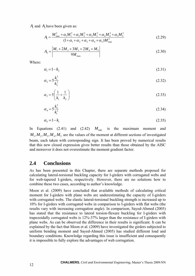
The values of the design buckling resistance obtained from hand calculations using formulas given in Eurocode3 and PN-90/B-03200 have been presented in Table 3.2 below.
Table 3.2 Design buckling resistance obtained from hand calculations.
Columns: Design buckling resistance Nb,Rd [kN] EN-1993-1-1:2005 PN-90/B-03200
Column 2m 3504 3660 Column 5m 2380 2502 Column 10m 972,6 921,5
As can be noticed, the results obtained from hand calculations using both codes do not differ significantly. For slender columns calculations based on PN-90/B-03200 have given the result which is more on the safe side while for intermediate and stocky columns the value of design buckling resistance has been smaller when calculated according to Eurocode3. In further discussion of the results only the ones obtained from procedures given by Eurocode 3 have been compared to the results obtained from Finite Element Analysis. It has been sufficient in the investigated case and more reasonable as long as performed Finite Element Analysis includes methodologies proposed by Eurocode3.
3.1.2 Finite Element Analysis of design buckling resistance The second method to calculate the design buckling resistance of columns subjected to compression combines the methodology presented in Eurocode3 with the use of second-order analysis. In the investigated cases the commercial software package ABAQUS has been used to perform these analyses.
For the purpose of this studeis 3D models consisted of Wire Planar type element have been used. Three columns of lengths equal to two, five and ten meters have been modelled. Two beam element types have been analyzed and compared, namely ‘Euler-Bernoulli’-type beam element B33 and ‘Timoshenko’-type beam element B31OS. According to the ABAQUS User’s Manual, the first one is recommended to analyse slender columns while the second one can be applicable to thick as well as slender columns. Every element has been analyzed by meshing with the deviation factor equal to 0,1. The default number of integration points has been adopted, which is a three-point Simpson integration scheme for each segment making up the section. Buckling of columns consisted of a profile pictured in Figure 3.1 has been analysed. Material properties which have been used in all models correspond to the ones presented in the beginning of Chapter 3.
All investigated columns have been simply supported with fixed rotation around Y axis (UR2) in order to ensure in-plane buckling mode. Columns are centrally loaded and subjected to compression.

CHALMERS, Civil and Environmental Engineering, Master’s Thesis 2009:NN 19
The boundary conditions and the applied load for this case have been shown in Figure 3.2 below.
Figure 3.2 Boundary conditions and applied load.
As a first step linear buckling analysis has been performed. By using this type of analysis the linear buckling load capacity can be estimated. This method assumes small deformation before the collapse. In the first order analysis the initial geometry of the structure has been used. The linearized eigenvalue problem can be stated as:
( ) 0GK Kλ φ− = (3.9)
The buckling load capacity has been obtained by multiplying the value of applied reference load by obtained eigenvalue as follows:
cr refP Pλ= (3.10)
Usually the first eigenvalue and eigenmode are of interests.
By performing linear Finite Element Analysis buckling capacity has been obtained for both beam element types: B33 and B31OS. All results have been collected in Table 3.3 below.
Table 3.3 Theoretical buckling load: Euler’s Theory vs. Finite Element Analysis
Columns: The buckling load Pcr [kN] Euler's Theory FEA - B33 FEA -B31OS
Column 2m 32650 32644 30048 Column 5m 5224 5223 5152 Column 10m 1306 1305,7 1301,3

CHALMERS, Civil and Environmental Engineering, Master’s Thesis 2009:NN 20
The results obtained from Finite Element Analysis have given a good accuracy in comparison to the results calculated by hand calculations using Euler’s theory. Since beam element type B33 is based on Euler’s theory, the values of the buckling load are almost equal to the theoretical ones. However, values of the buckling load for a beam element type B31OS differ insignificantly from the theoretical ones, they have the same magnitude which confirms that they are also valid.
In the calculations above the case of ‘perfect’ columns has been analysed. In reality structures would never reach this magnitude of load due to its material properties, geometrical imperfections, residual stresses and other circumstances. This analysis has theoretical value and moreover it in Finite Element Analysis it is a basis to perform a second order non-linear analysis described in the following Section of this report.
Second step of Finite Element Analysis which has been performed is a non-linear analysis. For this case step module Static Risks, which computes buckling load capacity, has been used. It takes into account second order effects, material non-linearities and it implies initial imperfection and residual stresses by applying initial bow imperfection as has been pictured in Figure 3.3. The value of this bow imperfection has been calculated from Table 5.1 from Eurocode3. It depends on the length of a member, which is analysed and on the buckling curve corresponding to the investigated section.
Figure 3.3 Initial bow imperfection.
In the second step two kinds of analyses have been performed, namely for elastic and plastic material model. In the elastic analysis material non-linearities and initial imperfections have been taken into account. In the plastic analysis the same criteria have been implied and moreover material properties have been added.
eo - local bowimperfection

CHALMERS, Civil and Environmental Engineering, Master’s Thesis 2009:NN 21
The plastic material model which has been adopted is presented in Figure 3.4 below.
Figure 3.4 Stress-strain curve.
From the non-linear analysis the results obtained for beam element type B33 and B31OS have given compatible results. Therefore it has been sufficient to discuss only the results for one of these beam element types, which has been made in the following Section of this report.

CHALMERS, Civil and Environmental Engineering, Master’s Thesis 2009:NN 22
3.1.3 Results and discussion In this Section in-plane buckling of a centrally loaded column in compression has been analysed by both non-linear Finite Element Analysis and theoretical calculations. In both cases initial imperfections and material nonlinearities have been taken into account as described before.
The first column which has been analysed is a case of a stocky column with the relative slenderness equal to 0,34λ = and the buckling reduction factor equal to
0,929ϕ = . It is the case when a member is not sensitive to a loose of stability and the failure occures due to yielding. Theoretical value of critical force for a stocky column with length equal to 2m is very large. In reality such magnitude of the load would never be reached as long as the failure due to yielding would occur at a load level approximately ten times lower than the buckling load. Initial imperfections which have been applied in this case are equal to 10mm. The results obtained from elastic material model analysis has been shown in Figure 3.5 below.
Figure 3.5 Load-displacement chart: elastic analysis of the cloumn of length L1=2m.
In the beginning of the analysis the load-displacement curve has been linear and while the load has been increasing it has changed its shape. It has bended and has got closer to the theoretical value of the buckling load. Finite Element Analysis has stopped when the program has noted the negative eigen value, which means that at that load level the buckling has occured. Initial imperfections and material non-linearities can explain why the theoretical value of a buckling load obtained from Finite Element Analysis is lesser than the theoretical value calculated according to Euler’s theory. Moreover a stocky column is maybe not the best exapmle to ilustrate the buckling behaviour of columns.
10
28469,80
32650 32650
2948 29480
5000
10000
15000
20000
25000
30000
35000
0 20 40 60 80 100
Reaction
Force [k
N]
Displacement U3 [mm]
Column 2m ‐ Elastic Model
Reaction force vs U3Pcr Euler
Yielding FEA

CHALMERS, Civil and Environmental Engineering, Master’s Thesis 2009:NN 23
The second column which has been analysed is a case of an intermediate column with the relative slenderness equal to λ = 0,85 and the buckling reduction factor equal to
0,631ϕ = . In this case a member is also rather not sensitive to a stability loose and a failure of the element is governed by yielding. Theoretical value of buckling load for intermediate columns is also rather large. In reality such magnitude of the load would not be reached as long as the failure due to yielding would occure at a load level approximately two and a half times lower than the buckling load. Initial imperfections which have been applied in this case are equal to 25mm. The results obtained from elastic material model analysis can be seen in Figure 3.6 below.
Figure 3.6 Load-displacement chart: elastic analysis of the cloumn of length L2=5m.
As can be observed from the chart above, the load-displacement curve first has been linear, then it has bended and got asymptotic to the value of a critical load. Further on. buckling has occured and the analysis has finished.
The results obtained from Finite Element Analysis have given a good accuracy to the theoretical values of the bucklng load. The behaviour of the investigated element in Finite Element Analysis has been as expected, which confirms its corectness.
25
4985,01
52245224
1894,85 1894,85
0
1000
2000
3000
4000
5000
6000
0 100 200 300 400 500
Reaction
force [kN]
Displacement U3 [mm]
Column 5m ‐ Elastic Model
Reaction force vs U3Pcr Euler
Yielding FEA

CHALMERS, Civil and Environmental Engineering, Master’s Thesis 2009:NN 24
The third column which has been analysed is a case of a slender column with the relative slenderness equal to 1,7λ = and the buckling reduction factor equal to
0,258ϕ = . This column is more sensitive to the instability than the ones described before. It is an example when the failure is governed both by the losse of stability and material failure due to yielding. Here the difference between the magnitude of the load when the buckling occurs and the load magniture when a member yields is not so significant as in the examples of two-meter and five-meter columns. Initial imperfections which have been applied in this case are equal to 50mm. The results obtained from elastic material model analysis has been pictured in Figure 3.7 below.
Figure 3.7 Load-displacement chart: elastic analysis of the cloumn of length
L3=10m.
As can be observed from the chart above, the load-displacement curve first has been linear, then it has bended and got asymptotic to the value of the critical load. Then the buckling has occured and the analysis has finished. The reason why the load-displacement curve has reached the value which is larger than the value of the critical load can be explained by the step size or by the fact that theoretical calculations for slender elements are more on the safe side. Generally the results obtained from Finite Element Analysis have given a good accuracy to the theoretical values of the buckling load. The behaviour of the investigated element in Finite Element Analysis has been as expected, which confirms its corectness.
50
1339,85
1306 1306
835,8 835,8
0
200
400
600
800
1000
1200
1400
1600
0 500 1000 1500 2000 2500
Reaction
force [kN]
Displacement U3 [mm]
Column 10m ‐ Elastic Model
Reaction force vs U3Pult EC3
Yielding FEA

CHALMERS, Civil and Environmental Engineering, Master’s Thesis 2009:NN 25
Next analysis which has been performed is a non-linear analysis additionally taking into account plastic material properties of all considered elements. Material plastic model from Figure 3.4 has been implied. Consequently buckling resistance has been obtained and compared to the values of ultimate load calculated using procedures from Eurocode3.
The first column which has been analysed is a case of a stocky column. The results obtained from plastic material model analysis can be seen in Figure 3.8 below.
Figure 3.8 Load-displacement chart: plastic analysis of the cloumn of length L1=2m.
As can be observed from the chart above, the results obtained from Finite Element Analysis are comparable to the expected values obtained from hand calculations. The load-displacement relations have risen linearly until stresses in the sections have reached the value of the yield strength, which is 355MPa in the investigated case. After yielding the load could still be increased since stress distribution in the section has been possible. Horizontal displacement has been very small in this case and equal to: 10mm due to input initial imperfections and around 2mm due to displacement caused by the applied load. Failure has been governed only by yielding.
3361,03
3504 3504
3260,68 3260,68
0
500
1000
1500
2000
2500
3000
3500
4000
0 5 10 15 20
Reaction
force [kN]
Displacement U3 [mm]
Column 2m ‐ Plastic Model
Reaction force vs U3
Pult EC3
Yielding

CHALMERS, Civil and Environmental Engineering, Master’s Thesis 2009:NN 26
The second column which has been analysed is a case of an intermediate column with section properties as described before. As previously the non-linear analysis adopting platic material model has been performed taking into account second order effects, initial imperfections, residual stresses and material non-linearities. The results obtained from plastic material model analysis have been shown in Figure 3.9 below.
Figure 3.9 Load-displacement chart: plastic analysis of the cloumn of length L2=5m.
As can be observed from the chart above, the results obtained from Finite Element Analysis have given a good accuracy to the expected values obtained from calculations based on Eurocode3. The load-displacement relations have risen linearly until stresses in the sections have reached the value of the yield strength, which is 355MPa in the investigated case. At this point failure of the element can be captured. There has been no further stress distribution in the section. Horizontal displacement in this case has been equal to: 25mm due to input initial imperfections and around 30mm due to displacement caused by the applied load. Consequently, second order effects have occurred, which need be taken into account in the analysis. This phenomenon has been described in a more detailed manner in the following part of this report. In this case failure also has been governed by yielding.
25
2194,38
2380 23802198,77 2198,77
0
500
1000
1500
2000
2500
0 20 40 60 80
Reaction
force [kN]
Displacement U3 [mm]
Column 5m ‐ Plastic Model
Reaction force vs U3
Pult EC3
Yielding FEA

CHALMERS, Civil and Environmental Engineering, Master’s Thesis 2009:NN 27
The third column which has been analysed is a case of a slender column. As previously the non-linear analysis adopting platic material model form Figure 3.4 has been performed. Second order effects, initial imperfections, residual stresses and material-non-linearities have been also taken into account. The results obtained from plastic material model analysis can be seen in Figure 3.10 below.
Figure 3.10 Load-displacement chart: plastic analysis of the cloumn of length
L3=10m.
As can be observed from the chart above, the results obtained from Finite Element Analysis also have given a good accuracy to the expected values obtained from hand calculations. The load-displacement relations first have raised linearly, then the curve has bended until stresses in the sections have reached the value of the yield strength, which is 355MPa in the investigated case. At this point failure of the element can be captured. There has been no further stress distribution in the section. From the shape of this load-displacement chart it can be inferred that the factors which have influenced the failure of the element have been both yield strength of the section and the fact that it is slender and sensitive to stability loose. Horizontal displacement in this case has been equal to: 50mm due to input initial imperfections and around 130mm due to displacement caused by the applied load. Consequently, second order effects have occurred, which are significant and need be taken into account. This phenomenon has been described in details in the following part of this report
865,68 870,61
972,65 972,65
887,72887,72
0,00
200,00
400,00
600,00
800,00
1000,00
1200,00
0,00 50,00 100,00 150,00 200,00 250,00 300,00
Reaction
force [kN]
Displacement U3 [mm]
Column 10m ‐ Plastic Model
Reaction force vs U3Pult EC3
Yielding FEA

CHALMERS, Civil and Environmental Engineering, Master’s Thesis 2009:NN 28
What has been interesting in all cases is the load-point when the yielding has occurred. For different types of columns different distribution of initial forces can be observed. Consequently, failure of the element has been governed by different factors. Having this kind of knowledge is important to understand the behaviour of various types of columns. In all investigated cases yielding has occurred when stress distribution in the section has reached the yield strength which for applied material properties in the investigated case is equal to 355MPa.
Figures which have been presented in this Section of the report are supposed to illustrate the stress distribution at the point when yielding in the first fibres has occurred. Moreover, it has shown the distribution due to compressive force compared to the distribution due to second order moment.
For the first considered case of stocky column stress distribution in the section has been presented in Figure 3.11 below.
Figure 3.11 Stress distribution while yielding in the column of length L1=2m.
As can be observed from the drawing above, the factor which has governed the failure due to yielding is a compressive force. Contribution of a moment has been much smaller. In this case of stocky columns second order effects have no significant influence, therefore they could be neglected. The reason why there has been a small contribution from a moment is the presence of initial imperfections equal to 10mm, which have been input in the second order analysis. In this case the whole section has been in compression.
Values of compressive force and bending moment, as well as partial stresses caused by them have been pictured in Figure 3.11 above.

CHALMERS, Civil and Environmental Engineering, Master’s Thesis 2009:NN 29
The second column of interests has been an intermediate column. For this case a stress distribution in the section has been presented in Figure 3.12 below.
Figure 3.12 Stress distribution while yielding in the column of length L2=5m.
As can be observed from the drawing above, in the second case the factors which have governed the failure due to yielding are a compressive force and a second order moment. Contribution from both of them is comparable. In this case of intermediate columns second order effects have an influence on the behaviour of the column, thus they should be taken into account. In this case similarly as for the case of two-meter column the whole section has been in compression, although stress distribution in the section at the point of yielding has differed significantly.
Values of compressive force and bending moment, as well as partial stresses caused by them have been pictured in Figure 3.12 above.

CHALMERS, Civil and Environmental Engineering, Master’s Thesis 2009:NN 30
The last considered element has been a case of a slender column. For this case stress distribution in the section has been presented in Figure 3.13 as follows:
Figure 3.13 Stress distribution while yielding in the column of length L3=10m.
It can be noticed from the drawing above, that the factor which has governed the failure due to yielding is mainly a second order moment. In this case of a slender column second order effects have a significant influence on the behaviour of the column, thus they always should be taken into account. In this case in opposition to the cases described before, one part of a section has been in compression while the other part has been in tension. Stress distribution in the section at the point of yielding has differed significantly.
Values of compressive force and bending moment, as well as partial stresses caused by them have been pictured in Figure 3.13
In conclusion, Finite Element Analysis for all described models has given the results, which are comparable to the theoretical ones. This confirms the accuracy of the Finite Element models which have been used.

CHALMERS, Civil and Environmental Engineering, Master’s Thesis 2009:NN 31
3.2 Case study of beams subjected to uniform bending The second problem which has been analyzed is a case of a beams subjected to uniform bending. In this case lateral-torsional buckling resistance of a double symmetric cross-section has been analysed. It is a type of instability when a member, loaded by forces in plane of symmetry, deforms in this plane until reaching the buckling load. At this point a member deflects out of its plane and twists simultaneously. Lateral-torsional buckling differs from the column buckling because it occurs as an out-of-plane buckling mode. In case of columns the deformation caused by the loading and eventual buckled configuration are restricted to the same plane. Thus it can be defined as in-plane behaviour.
Lateral-torsional buckling is especially important in the design of beams without lateral supports. In this case the bending stiffness of the beam in the plane of loading is large in comparison to the lateral flexural rigidity. The beam becomes unstable if the load increases beyond the critical value. Lateral-torsional buckling risk should be taken into account particularly during the erection of the stricture, before the lateral restrains are installed.
In the linear analysis the instability can be captured at the maximum point on the load-deflection curve. In reality the value of ultimate moment does not coincide with the results obtained from the linear analysis. Material non-linearities, residual stresses and initial imperfections need to be taken into account, which influences the lateral-torsional resistance of a beam. Modern steel structures codes, which are based on a limit state concept, contain design procedures to calculate lateral-torsional buckling resistance of prismatic beams. As one of the first steps these procedures generally require the determination of the elastic critical buckling moment. Subsequently, by the use of buckling curves initial imperfections, residual stresses and inelastic buckling are taken into account.
Eurocode3 presents several alternative methods for obtaining lateral-torsional buckling resistance of members subjected to bending. In the investigated case two methods of hand calculations proposed by Eurocode3 have been compared with the third method using numerical methods and commercial Finite Element program ABAQUS. Two procedures for performing hand calculations are: a method proposed for a general case and a method proposed for rolled and equivalent welded sections. The third method adopts procedures given in parts 6.3.2 and 5.3.2 of Eurocode3 to carry out second order analysis. All methodologies take into account initial imperfections, material non-linearities and residual stresses, although in different ways.
In order to capture the behaviour of beams with different slenderness, parametric studies of three elements with various lengths have been carried out. The investigated beams have been two, five and ten meters long. This procedure allows gaining knowledge about the behaviour of beams with different slenderness, which fail in fundamentally different ways. Analyses have been carried out using two procedures suggested by Eurocode3 as well as numerical methods using software package ABAQUS. The results have been compared and commented.

CHALMERS, Civil and Environmental Engineering, Master’s Thesis 2009:NN 32
3.2.1 Hand calculations of lateral-torsional buckling resistance In order to estimate the design buckling resistance moment of a laterally unrestrained beam subjected to uniform bending Eurocode3 presents appropriate formulas to perform hand calculations. This is the easiest method, which does not require any specialized computer software and is very useful for design procedures. For the purpose of this studies lateral-torsional buckling resistance of three beams with cross-section shown in Figure 3.1, with lengths (L1=2m and L2=5m and L3=10m) has been calculated. Computer program MathCAD has been used for this purpose. Calculations from MathCAD can be found in Appendix B.
In the performed calculations beams have been assumed to be prismatic, simply supported and subjected to bending moment at both ends. Out-of-plane buckling has been studied. In this case bending occurs about the strong axis of the I-section.
In this Section the formulas given in Eurocode3 for two alternative methodologies have been presented and the results obtained from hand calculations have been compared and commented.
The first methodology which has been presented in Eurocode3 corresponds to a general case. This case is recommended for bending members of constant cross-section. Eurocode3 is considering lateral-torsional buckling of beams as an ultimate limit state related to member buckling resistance. To obtain this buckling resistance the resistance of the cross-section is multiplied by the reduction factor LTχ , which is defined as follows:
22
1 1LT
LTLT LT
χλ
= ≤Φ + Φ −
(3.11)
Where: 2
0,5[1 ( 0,2) ]LT LTLT LTα λ λΦ = + − + (3.12)
Reduction factor stated above takes into account two parameters, that is: the imperfection factor LTα and the non-dimensional slenderness LTλ defined as:
y yLT
cr
W fM
λ = (3.13)
The imperfection factor LTα takes into account the influence of the initial imperfections, residual stresses and other nonlinear effects and it corresponds to the appropriate buckling curve taken from Eurocode 3. Whereas LTλ is the non-dimensional slenderness and it is related to the elastic critical moment for lateral-torsional buckling crM . It should be pointed out that Eurocode3 does not provide any information how to compute crM . However, formulas for calculating the elastic critical moment for the simplest case of prismatic beam with plane webs can be found in separate sources. The method for calculating the elastic critical moment crMgiven in Access Steel SN003a-EN-EU (2007) is valid for double symmetric cross-sections with uniform straight members.

CHALMERS, Civil and Environmental Engineering, Master’s Thesis 2009:NN 33
The formula for the elastic critical moment has been derived from the buckling theory, as follows:
2 22 2
1 2 22 2
( )( ) ( )( )
y wcr g g
w y y
EI Ck kL GJM C C z C zkL k I EI
ππ
⎧ ⎫⎧⎪⎪ ⎪= + + −⎨⎨ ⎬⎪⎪ ⎪⎩⎩ ⎭
(3.14)
For uniform moment, with assumption that there are lateral restraints or when the force is applied in the shear centre crM is given as:
2 2
2 2y w
cry y
EI C L GJML I EI
ππ
= + (3.15)
The formula for elastic critical moment for the simplest configuration, of simply supported beam of constant section subjected to uniform moment has been also given by Galambos (1988) as follows:
20, (1 )cr yM EI GJ W
Lπ
= + (3.16)
Where:
wECWL GJπ
= (3.17)
Equations (2.5) and (2.6) are equivalent with an assumption that the ends of the beam are prevented from lateral deflection.
The warping constant wC in the above cases has been given as: 2 2( )
4 4y f y w
w
I h t I hC
−= = (3.18)
Having these data it is possible to calculate crM and then, by inserting it to
Equation (2.3), the non-dimensional slenderness LTλ . After selecting the proper buckling curve the initial imperfection factor LTα is obtained, which allows finding the reduction factor LTχ .Consequently, the design buckling resistance moment of a laterally unrestrained beam can be calculated using formula:
,b Rd LT y yM W fχ= (3.19)
Second methodology proposed by Eurocode3 and applicable in the investigated case is a method particularly recommended for rolled sections and equivalent welded sections in bending. It differs from the general case by the way how the reduction factor LTχ and the factor LTΦ are calculated. Formulas for these factors have been defined as:
22
1 1LT
LTLT LT
χβλ
= ≤Φ + Φ −
(3.20)

CHALMERS, Civil and Environmental Engineering, Master’s Thesis 2009:NN 34
Where: 2
,00,5[1 ( ) ]LT LT LTLT LTα λ λ βλΦ = + − + (3.21)
The parameters β and ,0LTλ which appear in the equations above, concerning the beam depth or h/b ratio, may be taken from National Annex. Eurocode3 recommends adopting 0,75β = and ,0 0, 4LTλ = as the most unfavourable case.
Moreover, the value of the imperfection factor differs as long as buckling curve is selected from other Table from Eurocode 3, i.e. Table 6.5.
Other formulas needed to calculate the design buckling moment of laterally unrestrained beams are the same as for the general case.
A comparison of obtained results of the buckling reduction factor and design buckling moment has been made in Table 3.4 and Table 3.5 below.
Table 3.4 Buckling reduction factor
Beams: Buckling reduction factor [-] EC3 General case EC3 Rolled sections
Beam2m 0,976 1 Beam 5m 0,845 0,867 Beam 10m 0,544 0,592
Table 3.5 Design buckling resistance obtained from hand calculations
Beams: Design buckling moment Mb,Rd [kNm] EC3 General case EC3 Rolled sections
Beam 2m 412,85 423,175 Beam 5m 357,628 366,825 Beam 10m 230,071 250,391
It can be observed that values of the design buckling moment of laterally unrestrained beams which have been obtained using second methodology are higher. Second method is recommended for rolled sections and equivalent welded sections, thus probably more accurate in the investigated case. On the other hand, general method is universal and gives the results which are more on the safe side. Both methodologies are also compared using Finite Element Analysis in the following Setion of this report.
3.2.2 Finite Element Analysis of lateral-torsional buckling resistance
The other method to calculate the design lateral-torsional buckling resistance of beams subjected to uniform bending combines the methodology presented in Eurocode3 with the use of second-order analysis. In the investigated cases the commercial software package ABAQUS has been used to perform these analyses.

CHALMERS, Civil and Environmental Engineering, Master’s Thesis 2009:NN 35
For the purpose of these studies 3D models consisted of Wire Planar type element have been used. Three beams of lengths equal to two, five and ten meters have been modelled. Beam element type B31OS have been adopted. According to the ABAQUS User’s Manual this is ‘Timoshenko’-type beam element. It is recommended for all types of beams with open sections. Every element has been analyzed by meshing with the deviation factor equal to 0,1. The default number of integration points has been adopted, which is a three-point Simpson integration scheme for each segment making up the section. Lateral-torsional buckling of beams consisted of a profile pictured in Figure 3.1 has been analysed. Material properties used in all models correspond to the ones presented in the beginning of Chapter 3.
All investigated beams have been simply supported. Beams have been subjected to uniform moment applied at both ends of the element. In Figure 3.14 the boundary conditions and the way the applied load has been shown.
Figure 3.14 Boundary conditions and applied load.
As a first step linear buckling analysis has been performed. By using this type of analysis the linear buckling load capacity can be estimated. This method assumes small deformation before the collapse. In the first order analysis the initial geometry of the structure has been used. The linearized eigenvalue problem can be stated as:
( ) 0GK Kλ φ− = (3.22)
The theoretical critical buckling moment has been obtained by multiplying the value of applied reference load by obtained eigenvalue as follows:
cr refM Mλ= (3.23)
Usually the first eigenvalue and eigenmode are of interests.
By performing linear Finite Element Analysis the theoretical lateral-torsional buckling capacity has been obtained. The results from Finite Element Analysis have been compared with the results obtained from hand calculations.

CHALMERS, Civil and Environmental Engineering, Master’s Thesis 2009:NN 36
All results have been collected in a Table 3.15 below.
Table 3.15 Theoretical critical buckling moment: Theory vs. Finite Element Analysis
Beams: The critical moment Mcr [kNm] Theory FEA -B31OS
Beam 2m 4459,0 4596,9 Beam 5m 850,02 878,46 Beam 10m 304,66 310,28
The results obtained from Finite Element Analysis have given a good accuracy in comparison to the results obtained from hand calculations, with an error around 3%.
In the calculations above the case of ‘perfect’ elements has been analysed. This means they have no initial imperfections, no residual stresses and no material-nonlinearities. In reality structures would never reach this magnitude of load due to its material properties, geometrical imperfections, residual stresses and other circumstances. This analysis has theoretical value and moreover it in Finite Element Analysis it is a basis to perform a second order non-linear analysis described in the following Section of this report.
Second step of Finite Element Analysis which has been performed is a non-linear analysis. For this case step module Static Risks, which computes the lateral-torsional buckling capacity, has been used. This analysis takes into account second-order effects, material non-linearities and it implies initial imperfection and residual stresses. In order to consider initial imperfections and residual stresses, in the case of lateral-torsional buckling of a member in bending, Eurocode3 suggests slightly different method than the one presented for columns. In the second order analysis it suggests adopting equivalent initial bow imperfections from Table 5.1 in Eurocode3, as in the case of columns, but also additionally multiplied by a factor k. The recommended value of this factor is equal to k=0,5. By applying this procedure it is not needed to consider any additional torsional imperfections. The initial bow imperfection has been presented in Figure 3.16. It depends on the length of a member, which is analysed and on the buckling curve corresponding to the investigated section.
Figure 3.16 Initial bow imperfection.
In the second step two kinds of analysis have been performed, namely for elastic and plastic material model. In the elastic analysis material non-linearities and initial imperfections have been taken into account. In the plastic analysis the same criteria have been implied and moreover material properties have been added. The plastic material model which has been adopted is the same as for columns and presented in Figure 3.4 in the previous Section.
eo - initial bowimperfection

CHALMERS, Civil and Environmental Engineering, Master’s Thesis 2009:NN 37
3.2.3 Results and discussion In this Section the lateral-torsional buckling of beams subjected to uniform bending has been analysed by both non-linear Finite Element Analysis and theoretical calculations. In both cases initial imperfections and material non-linearities have been taken into account as described before.
Two types of non-linear analysis have been performed, namely for the elastic and plastic material model. In the analysis with plastic material model two methods presented in Eurocode3 have been compared: a general case and a method recommended for rolled and equivalent welded sections. In the case of the analysis with elastic material model results for both methodologies have been very close to each other. Thus to make charts more understandable it has been sufficient to present only the results for the general case.
The results obtained from the non-linear analysis with elastic material model for all beams have been collected in Figures 3.17-3.19 below.
Relation between the moment and vertical displacement U2 for a stocky beam has been presented in Figure 3.17 below.
Figure 3.17 Moment vs vertical displacement chart: elastic analysis of the beam of
length L1=2m.
3,33
5323,9
4459
4593,2
429,771
0
1000
2000
3000
4000
5000
6000
0 50 100 150 200
Mom
ent [kN
m]
Displacement U2 [mm]
Beam 2m ‐ Elastic Model
M vs U2 ‐ FEA
Mcr ‐ Theory
Mcr ‐ FEA
Yielding ‐ FEA

CHALMERS, Civil and Environmental Engineering, Master’s Thesis 2009:NN 38
Relation between the moment and vertical displacement U2 for an intermediate beam has been presented in Figure 3.18 below.
Figure 3.18 Moment vs vertical displacement chart: elastic analysis of the beam of
length L2=5m.
Theoretical value of the buckling load for a stocky and intermediate beam is very large. In reality such magnitude of the load is never reached as long as the failure due to yielding would occur at a load level much lower than the buckling load. For the stocky beam yielding would occur at the load level approximately ten times lower than the buckling load. And for the intermediate beam yielding would occur at the load level approximately two and a half times lower than the buckling load. Stocky and intermediate beams are not sensitive to a loose of stability and in reality the failure would occure due to yielding.
8,333
980,711
850,024
878,46
369
0
200
400
600
800
1000
1200
0 50 100 150 200
Mom
ent [kN
m]
Displacement U2 [mm]
Beam 5m ‐ Elastic Model
M vs U2 ‐ FEA
Mcr ‐ Theory
Mcr ‐ FEA
Yielding ‐ FEA

CHALMERS, Civil and Environmental Engineering, Master’s Thesis 2009:NN 39
Relation between the moment and vertical displacement U2 for a slender beam has been presented in Figure 3.19 below.
Figure 3.19 Moment vs vertical displacement chart: elastic analysis of the beam of
length L3=10m.
In case of a slender beam, as can be observed from Figure 3.17, the difference between the buckling load and the load at which the yielding occurs has been less significant than in cases of a stocky and an intermediate beam. Slender beams are much more sensitive to the loose of stabiility. The load level at which the yielding takes place is very close to the buckling load, thus these two factors interact.
In all investigated cases, in the beginning of the analyses the load-displacement curve has been linear and when the load has been getting closer to the theoretical buckling load, it has changes its shape. After reaching the theoretical critical buckling load post-buckling response can be observed in all cases. However, this response is decreasing as the slenderness of the beam is increasing. It can be explained by the way how ABAQUS is performing non-linear elastic analyses for this specific beam element type. The results from plastic non-linear analyses, presented in the following Section, have given a good accuracy to the expected values obtained from hand calculations, which confirm that the models have been modelled correctly.
Initial imperfections which have been applied in the investigated cases are equal to: 3,333mm for the two-meter-beam, 8,333mm for the five-meter-beam and 16,667mm for the ten-meter beam.
16,667
333,938
304,664310,28
283,81
0
50
100
150
200
250
300
350
400
0 100 200 300 400
Mom
ent [kN
m]
Displacement U2 [mm]
Beam 10m ‐ Elastic Model
M vs U2 ‐ FEA
Mcr ‐ Theory
Mcr ‐ FEA
Yielding ‐FEA

CHALMERS, Civil and Environmental Engineering, Master’s Thesis 2009:NN 40
Next analysis which has been performed is a non-linear analysis, additionally taking into account plastic material properties of all considered elements. Material plastic model from Figure 3.4 has been implied in all models. Consequently, lateral-torsional buckling resistance has been obtained and compared to the values of the design buckling resistance calculated using two procedures from Eurocode3.
The first beam which has been analysed is a case of a stocky beam. The results obtained from the analysis with plastic material model have been presented in Figure 3.20 and 3.21.
Relation between the moment and vertical displacement U2 for a stocky beam has been presented in Figure 3.20 below.
3.20 Moment vs vertical displacement chart: plastic analysis of the beam of length
L1=2m.
As can be observed from Figure 3.20, the results obtained from Finite Element Analysis have been comparable to the expected values obtained from hand calculations. The load-displacement relations have risen linearly until stresses in the sections have reached the value of the yield strength, which is 355MPa in the investigated case. After yielding the load could still be increased insignificantly since stress distribution in the section has been possible. Vertical displacement has been very small in this case and equal to: 3,33mm and 4mm due to input initial imperfections and around 6mm due to displacement caused by the applied load. In this case the failure has been governed only by yielding.
3,333
442,976
4
442,607429,771
412,85423,175
0
50
100
150
200
250
300
350
400
450
500
0 5 10 15
Mom
ent [kN
m]
Displacement U2 [mm]
Beam 2m ‐ Plastic Model
M vs U2 ‐ FEA 1st method
M vs U2 ‐ FEA 2nd method
Yielding FEA
Mult EC3 ‐ 1st method
Mult EC3 ‐ 2nd method

CHALMERS, Civil and Environmental Engineering, Master’s Thesis 2009:NN 41
Relation between the moment and horisontal displacement U3 for a stocky beam has been presented in Figure 3.21 below:
Figure 3.21 Moment vs horisontal displacement chart: plastic analysis of the beam of
length L1=2m.
In case of a stocky beam horizontal displacement has been very small, around 1mm. As expected, a stocky beam has not been sensitive to the lateral-torsional buckling. The failure ha been governed only by yielding. Results obtained from Finite Element Analysis have been very similar both when adopting the general case and the case of rolled sections presented in Eurocode3. Thus only one curve can be visible in Figure 3.21. In Figure 3.20 the shape of the curves has been also the same, however one is shifted since different initial imperfections have been applied. It can be concluded that a stocky beam is not sensitive for initial imperfections and loose of stability.
The results obtained from Eurocode3 are very close to the values obtained from Finite Element Analysis. Especially the second proposed method has given a good accuracy. In comparison: the error between hand calculations and Finite Element Analysis has been equal to 7% for the 1st method presented in Eurocode3 (a general case), and 4,4% for the 2nd method (for rolled and equivalent welded sections). The results which have been obtained from hand calculations are more conservative.
442,878442,607429,771
412,85
423,175
0
50
100
150
200
250
300
350
400
450
500
0 0,5 1 1,5
Mom
ent [kN
m]
Displacement U3 [mm]
Beam 2m ‐ Plastic Model
M vs U3 ‐ FEA 1st method
M vs U3 ‐ FEA 2nd method
Yielding FEA
Mult EC3 ‐ 1st method
Mult EC3 ‐ 2nd method

CHALMERS, Civil and Environmental Engineering, Master’s Thesis 2009:NN 42
The second beam which has been analysed is a case of an intermediate beam. The results obtained from the analysis with plastic material model have been presented in Figure 3.22 and 3.23
Relation between the moment and vertical displacement U2 for an intermediate beam has been presented in Figure 3.22 below.
Figure 3.22 Moment vs vertical displacement chart: plastic analysis of the beam of
length L2=5m.
As can be observed from the chart above, the results obtained from Finite Element Analysis have given a good accuracy with expected values obtained from hand calculations. The load-displacement relations have risen linearly until stresses in the sections have reached the value of the yield strength, which is 355MPa in the investigated case. After yielding the load could still be increased insignificantly since stress distribution in the section has been possible. Vertical displacement in this case has been equal to: 8,33mm/10mm due to input initial imperfections and around 30mm due to displacement caused by the load applied. In this case failure has been governed also by yielding.
8,333
393,918 386,361
366,825357,628
369
0
50
100
150
200
250
300
350
400
450
0 10 20 30 40 50 60
Mom
ent [kN
m]
Displacement U2 [mm]
Beam 5m ‐ Plastic Model
M vs U2 ‐ FEA 1st method
M vs U2 ‐ FEA 2nd method
Yielding FEA
Mult EC3 ‐ 1st method
Mult EC3 ‐ 2nd method

CHALMERS, Civil and Environmental Engineering, Master’s Thesis 2009:NN 43
Relation between the moment and horisontall displacement U3 for an intermediate beam has been presented in Figure 3.23 below:
Figure 3.23 Moment vs horisontal displacement chart: plastic analysis of the beam of
length L2=5m. In the case of an intermediate beam horizontal displacement has been also rather small, around 4mm. As expected, an intermediate beam is also not very sensitive to the lateral-torsional buckling. Results obtained from Finite Element Analysis have been very similar both when adopting the general case and the case of rolled sections presented in Eurocode3. Thus in the second case the value of the buckling resistance moment has been slightly lower, since larger initial imperfection has been applied. It can be concluded that an intermediate beam, is more sensitive to initial imperfections and loose of stability than a stocky beam. However, these factors have not governed the failure of a member. The failure has been governed by yielding
The results obtained from Eurocode3 are very close to the values obtained from Finite Element Analysis. Especially the second proposed method has given a good accuracy. An estimation of the point when yielding has occurred is very good in this case.
In comparison: the error between hand calculations and Finite Element Analysis has been equal to 9% for the 1st method presented in Eurocode3 (a general case), and 4,5% for the 2nd method (for rolled and equivalent welded sections). The results obtained from hand calculations have been more on the safe side.
393,918386,361
369
357,628
366,825
0
50
100
150
200
250
300
350
400
450
0 2 4 6 8 10 12 14
Mom
ent [kN
m]
Displacement U3 [mm]
Beam 5m ‐ Plastic Model
M vs U3 ‐ FEA 1st method
M vs U3 ‐FEA 2nd method
Yielding FEA
Mult EC3 ‐ 1st method
Mult EC3 ‐ 2nd method

CHALMERS, Civil and Environmental Engineering, Master’s Thesis 2009:NN 44
The third beam which has been analysed is a case of a slender beam. For this case the results obtained from the analysis with plastic material model have been presented in Figure 3.24 and 3.25
Relation between the moment and vertical displacement U2 for a slender beam has been presented in Figure 3.24 below.
Figure 3.24 Moment vs vertical displacement chart: plastic analysis of the beam of
length L3=10m.
The load-displacement relations have risen linearly until stresses in the sections have reached the value of the yield strength, which is 355MPa in the investigated case. Exactly when reaching the yield point the failure has occurred. Stress distribution in the section in this case has not been possible. As can be observed from the chart above, the results obtained from Finite Element Analysis have given quite good accuracy with expected values obtained from hand calculations. However, in this case the difference between them has been larger than in the cases of a stocky and intermediate beam Vertical displacement in this case has been equal to: 16,667mm/20mm due to input initial imperfections and around 110mm due to displacement caused by the load applied. In this case failure has been influenced both by yielding and by the loose of stability.
16,667
283,815
20
275,863
283,8
230,071
250,391
0
50
100
150
200
250
300
0 50 100 150 200
Mom
ent [kN
m]
Displacement U2 [mm]
Beam 10m ‐ Plastic Model
M vs U2v ‐ FEA 1st method
M vs U2 ‐ FEA 2nd method
Yielding FEA
Mult EC3 ‐ 1st method
Mult EC3 ‐ 2nd method

CHALMERS, Civil and Environmental Engineering, Master’s Thesis 2009:NN 45
Relation between the moment and horisontal displacement U3 for a slender beam has been presented in Figure 3.25 below.
Figure 3.25 Moment vs horisontal displacement chart: plastic analysis of the beam of
length L3=10m.
In the case of a slender beam a horizontal displacement has been larger than in the other cases and it has been equal almost 40mm. Results obtained from Finite Element Analysis have been very similar both when adopting the general case and the case of rolled sections presented in Eurocode3. Thus in the second case the value of the buckling resistance moment has been slightly lower, since larger initial imperfection has been applied.
It can be concluded that a slender beam, has been most sensitive to initial imperfections and loose of stability in comparison with the other investigated beams. The failure has been governed both by yielding and by the loose of stability.
In the case of a slender beam the results obtained from Eurocode3 are not so close to the values obtained from Finite Element Analysis as in the previous cases. Again the 2nd method proposed by Eurocode3 (for rolled and equivalent welded sections) have given better accuracy than the 1st method (a general case).
In comparison: the error between hand calculations and Finite Element Analysis has been equal to 19% for the 1st method presented in Eurocode3 (a general case), and 10% for the 2nd method (for rolled and equivalent welded sections). The results obtained from hand calculations have been much more on the safe side.
283,815
275,863
283,8
230,071
250,391
0
50
100
150
200
250
300
0 20 40 60 80
Mom
ent [kN
m]
Displacement U3 [mm]
Beam 10m ‐ Plastic Model
M vs U3 ‐ FEA 1st method
M vs U3 ‐ FEA 2nd method
Yielding FEA
Mult EC3 ‐ 1st method
Mult EC3 ‐ 2nd method

CHALMERS, Civil and Environmental Engineering, Master’s Thesis 2009:NN 46
4 Parametric studies of the I-section with corrugated web
In order to gain deeper knowledge about the problem of lateral-torsional buckling of I-girders with corrugated webs under uniform bending parametric studies have been performed. Three calculation models for obtaining theoretical critical moment have been compared, namely: the one proposed by NCCI (2007), second proposed by Lindner (1997) and third, most recent, proposed by Moon et al. (2009). MathCAD has been used to perform all calculations. Calculations can be found in Appendix C.
Eurocode3 does not provide any formulas for obtaining theoretical critical moment; however, it is using it to obtain the slenderness in the procedure of calculating lateral-torsional buckling resistance moment. Design codes, like NCCI (2007) in this case, give only formulas for theoretical critical moment for the simplest case of prismatic, simply supported beams subjected to uniform moment and restrained against lateral defection. There is lack of information in the available design codes how to deal with more complex examples. Further investigations should be performed.
In the parametric studies which have been carried out parameters which have been changing in all examples are: the depth of the beam hw and the thickness of the corrugated web tw. Investigated I-girder and the corrugation of the web have been shown in Figure 4.1.
Figure 4.1 The dimensions of the investigated profile.
Methodologies proposed by NCCI (2007), Lindner (1997) and Moon et al. (2009) for obtaining the elastic critical moment have already been presented in Chapter 2 and Chapter 3. Formulas for the elastic critical moment can be found in equations (2.13), (3.14) and (3.15) of this report.

CHALMERS, Civil and Environmental Engineering, Master’s Thesis 2009:NN 47
The results obtained from calculations using computer program MathCAD have been collected in Tables 4.1-4.3 below.
Methodology presented in NCCI (2007) assumes that the investigated beam is prismatic, has a flat web and that it is restrained against lateral torsion. The values of the theoretical critical moment, obtained using this method, have been presented in Table 4.1 below.
Table 4.1 Theoretical critical buckling moment: NCCI (2007).
Mcr – flat web hw = 2mm hw = 3mm hw = 4mm hw = 400mm 184,264 184,591 185,227 hw = 600mm 226,472 226,872 227,648 hw = 800mm 274,865 275,304 276,157
Methodology presented by Lindner (1997) deals with the case of the simply supported beam which is prismatic and has a trapezoidally corrugated web. The beam is subjected to uniform bending. This method applies the formula for the warping constant for the I-section with corrugated web from Equation (2.4). The values of the theoretical critical moment, obtained using this method, have been presented in Table 4.2 below.
Table 4.2 Theoretical critical buckling moment: Lindner (1997).
Mcr – Lindner hw = 2mm hw = 3mm hw = 4mm hw = 400mm 226,887 245,632 263,23 hw = 600mm 278,488 301,355 322,814 hw = 800mm 332,479 358,028 382,088
Methodology presented by Moon et al. (2009) deals with the case of the simply supported beam which is prismatic and has a trapezoidally corrugated web. The beam is subjected to uniform bending. This method applies the formula for the warping constant from Equation (2.10). The values of the theoretical critical moment, obtained using this method, have been presented in Table 4.2 below.
Table 4.3 Theoretical critical buckling moment: Moon et al. (2009).
Mcr – Moon et al. tw = 2mm tw = 3mm tw = 4mm hw = 400mm 178,993 179,382 180,057 hw = 600mm 222,527 223,126 224,068 hw = 800mm 272,141 272,99 274,213
It can be observed from the tables above that the results obtained from the methodology proposed by Moon et al. (2009) have been slightly smaller than the ones obtained using the procedure for a flat web. According to the article of Moon et al. (2009) the results obtained using their methodology for I-girders with corrugated webs should be larger than for the case of flat webs. They have proven it using Finite Element Analysis. The accuracy of Finite Element model used by Moon et al. has been validated by the comparison of the obtained theoretical critical moment with theoretical values.

CHALMERS, Civil and Environmental Engineering, Master’s Thesis 2009:NN 48
The results have been presented in Figure 4.2 below.
Figure 4.2 Verification result of Finite Element model.
It has been proven by Moon et al. (2009) that for the profiles which they have investigated formulas proposed for flat webs have been less accurate than using their method. The parameters which they have investigated in Finite Element Analysis have been the warping constant and the shear modulus. The comparison of these parameters made by Moon et al. (2009) has been presented in Figure 4.3 below.
Figure 4.3 Variation of Cw,co/Cw, flat and Gco/G with corrugation angle θ. To illustrate how the warping constant and the shear modulus influence the value of the theoretical critical moment the variation of the critical moment of the girder with flat and with corrugated web has been presented in Figure 4.4 .

CHALMERS, Civil and Environmental Engineering, Master’s Thesis 2009:NN 49
Figure 4.4 Variation of Mocr/Mocr,flat with corrugation angle θ. The reason why in the parametric studies, which has been carried out, the results have been not as expected is that Moon et al. (2009) have used different dimensions of their profile. Thus the results for other magnitude of the dimensions may differ. The dimensions used by Moon et al. have been much larger and have been presented in Figure 4.5 below.
Figure 4.5 Dimensions of analysis model investigated by Moon et al. (2009).
In comparison, the results obtained using the methodology proposed my Lindner (1997) have been larger than using two other methodologies. However, the confirmation of the methodology proposed by Lindner (1997) by Finite Element Analysis has not been available to the author, thus it is difficult to relay on these method.
In conclusion, Moon and al. (2009) provides the results from Finite Element Analysis which confirm they calculation model. Thus the accuracy of their methodology for calculating the theoretical critical moment has been validated. According to the studies performed by Moon et al. (2009) a practical design procedures from NCCI (2007) and Eurocode3 can be applicable to the I-girders with corrugated webs.

CHALMERS, Civil and Environmental Engineering, Master’s Thesis 2009:NN 50
No matter how large are the dimensions of the investigated section, the corrugation has an influence on a value of the critical moment only when the corrugation angle is larger than 40o. Moreover, it has no significant meaning then this angle is less than 40o. When the corrugation angle is around 60o the value of the critical moment is increased of around 10%. When the corrugation angle is 45o the value of the critical moment is increased of around 5%.
By applying this new methodology proposed by Moon et al. (2009) for the case of not very big steel frames, obtained values of critical moment have been even slightly smaller than these obtained from calculations based on Eurocode3. In conclusion it is rather useless to adopt this new methodology in our case. The methodology for calculating the theoretical critical moment proposed for I-profiles with the flat webs is sufficient in the investigated case. When considering structures consisted of profiles with medium dimensions it is sufficient to base calculation on a procedures presented in NCCI (2007) and Eurocode3. They are applicable in the case of interests of this report. The new methodology proposed by Moon et al. (2009) is applicable and useful for large-scale structures which are consisted of profiles with big dimensions.
There are no Finite Element models available for structures with medium dimensions, consisted of tapered I-girders with trapezoidally corrugated webs. Further investigations should be carried out. It is difficult to say if the methodology proposed by Moon et al. (2009) or Lindner (1997) is applicable in our case. Finite Element Analysis should be performed.

CHALMERS, Civil and Environmental Engineering, Master’s Thesis 2009:NN 51
5 Frame analysis Previous Chapters of this report have focused on a stability of single members which have failed due to axial force and bending moment. In this Chapter the limit state of elastic frame buckling has been investigated and described. According to Galambos (1998) the principal mode of frame failure is instability. That is the reason why frame buckling must be taken into account as one of the possible limit states in the design of the final structure. Frame buckling is especially dangerous during the erection of a structure, when the bracing and the cladding has not been installed yet. Thus the erection process needs to be analysed at every step of it. In order to be able to design safe constructions it is essential to understand and recognize the behaviour of frames subjected to external loads.
Two kinds of frame behaviour considering instability can be distinguished, namely in-plane buckling and out-of-plane buckling. In-plane buckling mode can be described as the case when the frame buckles in the same plane as the applied load. This type of buckling has been shown in Figure 5.1 below.
Figure 5.1 Asymmetric mode (sway mode) and symmetric mode of in-plane buckling
For the case of in-plane buckling imperfections which mainly should be taken into account in the second order analysis are frame imperfections. They are applied as an initial sway or as a system of equivalent horizontal forces. For the case of in-plane buckling analysis Eurocode3 suggests methods for performing hand calculations and obtaining buckling lengths and buckling resistance; however, this issue is out of the scope of this report and has not been elaborated.
The mode of buckling which is of interests of this report is out-of plane buckling. Out-of-plane buckling mode, described also as lateral-torsional buckling, can be defined as a case when the frame buckles out of the plane in which the load is applied. Members in compression in the frame deflect out of this plane and twist simultaneously. For the case of lateral-torsional buckling initial imperfections also need to be considered. Geometrical imperfections of the frames result in spatial displacement from the beginning of loading. This causes additional moments from the second order effects, which need to be taken into account. In order to perform second order analysis which would take into account initial imperfections and material non-linearities Finite Element Analysis need to be performed. Furthermore, design procedures available in Eurocode3 does not treat the complex problem of the frames with tapered and corrugated webs, thus Finite Element Analysis is the only reasonable solution to obtain accurate results.

CHALMERS, Civil and Environmental Engineering, Master’s Thesis 2009:NN 52
In this Chapter Finite Element Analysis of two 3D steel frames has been presented accounting for lateral-torsional buckling. The first order and the second order analyses have been performed. Second order analysis is non-linear and it takes into account material non-linearities and initial member imperfections of the structure. It is the most exact method for obtaining buckling resistance of the frames with tapered and corrugated webs. Moreover, a comparison between the frame with corrugated webs and the frame with plane webs has been made, accounting for out-of-plane buckling. The most critical points in the structure have been investigated and the frame load capacity has been analysed. Such investigation allows gaining a deeper understanding of frame instability phenomenon. It also gives a good opportunity to compare and verify two types of the frames used recently by companies constructing steel structures.
5.1 Investigated models As has been mentioned in the previous Sections of this report, there are no clear procedures in the available codes, like Eurocode3, to deal with the cases of more complex frames. Thus Finite Element Analysis has been performed in order to be able to compare the lateral-torsional resistance of the frames consisted of corrugated and plane webs.
The parameter which has been investigated is the required distance between the purlins and lateral restraints. The purpose of the purlins is to prevent the lateral-torsional buckling of the upper flange of the rafter while the purpose of the lateral restrains is to prevent the lateral-torsional buckling of the lower flange of the rafter and of the inner flange of the column.
The frames which have been analysed are 7,6m high with a span of 21,3m. These dimensions have been based on the projects delivered by Borga Company and have been shown in Figure 5.2 below.
Figure 5.2 Dimensions of all analysed frames.
Material properties which have been adopted for all models:
• Steel grade: S355 • Yield strength: 355yf MPa= • Young Modulus: 206, 8E GPa= • Poisson’s ratio: 0,29ν =

CHALMERS, Civil and Environmental Engineering, Master’s Thesis 2009:NN 53
All models have been created in computer software Ideas. In this programme the geometry has been created and whole structure has been meshed using thin shell elements. The mesh element size which has been used is equal to 25 which is rather small and assures the accuracy of the analysis. When section properties have been defined all models have been exported do ABAQUS. In ABAQUS the boundary conditions and the loads have been defined and required analyses have been performed.
The first model which has been created is a case of the frame with corrugated webs. To create the geometry computer program Ideas has been used. The geometry of the first frame has been shown in Figure 5.3 below.
Figure 5.3 Analysed frame with corrugated webs.
Analogically the second model has been created using the same dimensions, section properties and material properties. The only difference is the web which in the second case has been plane. The geometry of the second frame has been shown in Figure 5.4 below.
Figure 5.4 Analysed frame with plane webs.
The model which has been presented above has been created only to illustrate the difference in the linear buckling behaviour of the frame with the thin web of 3mm in case then it is corrugated and in case when it is plane. It is important to keep in mind that in the constructions which are realized in reality plane webs are thicker and moreover stiffened by vertical stiffeners which are welded to the web and flanges.

CHALMERS, Civil and Environmental Engineering, Master’s Thesis 2009:NN 54
This is quite problematic and expensive solution. That is why the usage of the corrugated web has been suggested. It requires using special equipment for automatic welding, however it can be very beneficial in the overall, as has been explained in the first Chapters of this report. In order to model the frame with plane webs, which is used in practice in steel structures the third model has been created. In this case all dimensions have been the same as in the first model, only the web thickness has been increased from 3mm to 6mm in the column and the area in the corner of the frame, 5mm in the middle of the rafter and 4mm in the end of the rafter. Moreover, vertical stiffeners have been added along the webs. The geometry of the third frame has been shown in Figure 5.5 below.
Figure 5.5 Analysed frame with the plane web with vertical stiffeners
As long as the frames are is symmetric it has been sufficient to study only one half of the frame.
Boundary conditions which have been applied in all cases have been described as follows. At the first support, in the bottom of the column, displacements about directions X, Y and Z and the rotation about direction y have been fixed at the point in the middle of the web. Moreover displacement about X direction has been restrained along the nodes of the edge of the web. Finally, displacement about Z direction has been fixed along the nodes of the edge of the flanges.
At the second support at the end of the rafter the displacement at each node along the edge has been prevented about X direction. Moreover displacement about Z direction has been prevented along the web.
In order to prevent tilting of the frame additional boundary condition had been added in the corner of the frame. The displacement in the Z direction has been fixed.
Load case which had been investigates is the major load case of self weight and snow load. It has been checked by the additional software programme to be the most critical load case accounting for lateral torsional buckling of the investigated frames. Thus it is sufficient for the purpose of this report. If more detailed analysis would be required it would be recommended also to consider the case of the wind load and other load combinations.

CHALMERS, Civil and Environmental Engineering, Master’s Thesis 2009:NN 55
Boundary conditions and the load which has been applied have been shown in Figure 5.6 below.
Figure 5.6 Boundary conditions and applied load.

CHALMERS, Civil and Environmental Engineering, Master’s Thesis 2009:NN 56
5.2 Results and discussion For all of the models described previously first order analysis has been performed using ABAQUS. The step which has been used for this purpose is Linear Buckling. After that, the second order analysis has been performed for the first and the third model. The step which has been used for this purpose is Static Riks. Moreover, parametric studies have been carried out regarding lateral restraints, both for the frame with the corrugated web and for the frame with the plane web with vertical stiffeners. The results from linear and non-linear analyses have been presented and compared in the following Section.
5.2.1 Linear buckling analysis As a first step of this investigation linear buckling analyses of all models have been performed. The load which has been applied in the linear analysis has been taken as 10kN/m.
The first buckling mode which has been obtained from the linear buckling analysis in the case of the frame with corrugated webs has been observed as buckling of the plane plate in the corner of the frame. The second buckling mode has been the lateral-torsional buckling mode. For the frame with corrugated webs eigen value obtained from linear buckling analysis for the second mode has been equal to 2,679 which corresponds to the load of 26,79kN/m.
In order to avoid this buckling mode and the problem of yielding in this area in further analyses, the thickness of this plate has been increased from 6mm to 8mm. Such change has been sufficient to obtain the lateral-torsional buckling mode as a first one, which has been of the interests of this report.
After increasing the thickness of the plate in the corner eigen value obtained from the linear buckling analyses has been slightly higher. For the frame with corrugated webs eigen value has been equal to 2,8812 which corresponds to the load of 28,812kN/m. The buckling mode for this case has been shown in Figure 5.7 below with deformation scale factor equal to 300.
Figure 5.7 Lateral-torsional buckling mode of the frame with corrugated webs.

CHALMERS, Civil and Environmental Engineering, Master’s Thesis 2009:NN 57
As can be observed form Figure 5.7 above, parts of the frame which have buckled are the inner flange of the column, the inner flange of the rafter near the corner of the frame and the outer flange of the rafter near the middle of the frame. In order to prevent these parts to buckle lateral restrains of the inner flanges should be added and for the outer flange the purlins should be installed.
For the second model with thin plane web the eigen value which has been obtained has been much lower than in the case of the frame with corrugated web. It has been equal to 0,8774 which corresponds to the load of 8,774kN/m . It can be clearly visible that the frame with corrugated webs has significantly higher value of buckling resistance than the frame with plane webs. Moreover, for the frame with plane webs, first 22 buckling modes have been caused by the shear buckling of slender webs. While in the case of the frame with corrugated web the first relevant buckling mode has been caused by the lateral-torsional buckling.
The buckling mode for the second model has been shown in Figure 5.8 below with deformation scale factor equal to 200.
Figure 5.8 Shear buckling of the thin, plane web.
In order to prevent the failure caused by shear buckling of the webs in the third model the thickness of the webs has been increased and vertical stiffeners have been added. In this way shear buckling of the web has been prevented and the eigen value and buckling mode obtained from the linear buckling analysis have been analogical to the ones obtained from the analysis of the first frame with corrugated webs.
The first buckling mode which has been obtained from the linear buckling analysis for the case of the frame with plane webs with vertical stiffeners has been observed as buckling of the plane plate in the corner of the frame. The second buckling mode has

CHALMERS, Civil and Environmental Engineering, Master’s Thesis 2009:NN 58
been the lateral-torsional buckling mode, analogically as for the first model. For the frame with plane webs with vertical stiffeners eigen value obtained from linear buckling analysis for the second mode has been equal to 2,796 which corresponds to the load of 27,96kN/m.
In order to avoid this buckling mode and the problem of yielding in this area in further analyses, the same as for the first model, the thickness of this plate has been increased from 6mm to 8mm. Such change again has been sufficient to obtain the lateral-torsional buckling mode as a first one. The increased thickness of the plane plate in the corners of both frames has been adopted in further non-linear analyses.
As a result eigen value obtained from the linear buckling analyses has been slightly higher. For the frame with corrugated webs eigen value has been equal to 2,876 which corresponds to the load of 28,76kN/m. The buckling mode for the third model has been presented in Figure 5.9 below with deformation scale factor equal to 300.
Figure 5.9 Lateral-torsional buckling mode of the frame with plane webs with
vertical stiffeners.
As can be observed form Figure 5.9 above, parts of the frame which have buckled are mainly the inner and the outer flange of the rafter and the inner flange of the column. This shape of buckling mode is additionally governed by the fact that a part of the vertical stiffeners in the rafter has been welded only on the one side of the web. In order to prevent these parts to buckle lateral restrains of the inner flange should be added and for the outer flange the purlins should be installed.
It can be noticed that the buckling load for the frame with corrugated webs and for the frame with plane webs with vertical stiffeners has been very similar, around 29kN/m. This means that the thin, corrugated web is a good substitute to the thicker plane with vertical stiffeners. For the frame with plane, thin web this load has been only equal to around 9kN/m.

CHALMERS, Civil and Environmental Engineering, Master’s Thesis 2009:NN 59
5.2.2 Non-linear buckling analysis As the next step non-linear Finite Element Analysis has been performed. For this purpose Static Riks analysis has been adopted. In this step material non-linearities and member imperfections have been introduced. Member imperfections have been taken into account by incorporating the initial bow imperfection. The shape of the imperfection has been taken from the first buckling mode from the linear analysis and the magnitude of this imperfection has been calculated according to Eurocode3. The value ,o de of the bow imperfection given in Table 5.1 in Eurocode3 has been based on a dimension of the longest member in the analysed model. For second order analysis, taking into account lateral-torsional buckling of a member in bending, Eurocode3 gives the value of initial imperfection as ,o dke . The coefficient k is recommended to be taken as equal to 0,5. This method allows disregarding an additional torsional imperfection. By following this procedure the value of initial imperfection obtained for the investigated frame has been equal to 37,4mm.
The failure point which has been analysed in the models has been defined as the point when stresses in the members exceed the yield stress equal to 355MPa. Second order analysis has been performed for the case of the first and the third analysed model. This has been done because the second model of the frame with thin, plane web has been presented only to show the differences in linear buckling behaviour of investigated models.
The arbitrary load which has been applied has been equal to 5kN/m. The steps which have been defined in the Static Riks analysis have been fixed and taken as equal to 0,2. This value is rather small in order to capture the differences between the investigated frames.
The first analysis which has been performed has corresponded to the case of the frame without any restraints: no purlins and no lateral restraints of the inner flanges. This analysis has been performed both for the frame with corrugated webs and for the frame with plane webs.
For the case of the frame with corrugated webs yielding of first fibres has been observed at one node at the connection between the column and the rafter at load level of 15kN/m, which correspond to the reaction force equal to 165kN. When the load has approached 15,6kN/m yielding has been captured also to the inner flange of the column. For this case the reaction force has been equal to 171,8kN. High stresses concentration at only one node could be caused by different aspects, i.e. simplified model of the connection, big difference between the thicknesses of connecting elements, possibility of the forced position of the nodes in this area, due to merging while meshing in Ideas. That is why it is more reliable to take the second mentioned value of the load level as the load level where yielding has occurred.

CHALMERS, Civil and Environmental Engineering, Master’s Thesis 2009:NN 60
The area of yielding has been pictured in Figure 5.10 below.
Figure 5.10 The area of yielding for the frame with corrugated webs without any
lateral restraints.
The in-plane deflection of this model has been illustrated in Figure 5.11 below.
Figure 5.11 In-plane deflection of the frame with corrugated webs without any lateral
restraints.

CHALMERS, Civil and Environmental Engineering, Master’s Thesis 2009:NN 61
The out-of-plane deflection of this model has been illustrated in Figure 12 below.
Figure 5.12 Out-of-plane deflection of the frame with corrugated webs without any
lateral restraints.
In this case, in-plane deflection in U1 direction has been equal to 22mm. Out-of plane deflection in U3 direction has been equal to 39mm for the inner flange of the rafter, 33mm for the outer flange of the rafter and 19mm for the inner flange of the column.
In the case of the frame with plane webs with vertical stiffeners, the first points of yielding have been captured at one node at the connection of the stiffener in the corner of the frame at load level of 14,8kN/m, which corresponds to the reaction force equal to 162,8kN. When the load has approached 16,24kN/m yielding has been captured also to the inner flange of the column. In this case the reaction force has been equal to 178,6kN. Again the second load level is considered as more reliable. The reason of this fact has been explained before.

CHALMERS, Civil and Environmental Engineering, Master’s Thesis 2009:NN 62
The area of yielding for the frame with plane webs has been pictured in Figure 5.13 below.
Figure 5.13 The area of yielding for the frame with plane webs without any lateral
restraints.
The in-plane deflection of this model has been illustrated in Figure 5.14 below.
Figure 5.14 In-plane deflection of the frame with plane webs without any lateral
restraints.

CHALMERS, Civil and Environmental Engineering, Master’s Thesis 2009:NN 63
The out-of-plane deflection of this model has been illustrated in Figure 5.15 below.
Figure 5.15 Out-of-plane deflection of the frame with plane webs without any lateral
restraints.
The shape of in-plane deflection has been very similar in every case, which is why the figure showing this deflection has not been repeated in the following paragraphs; only the proper magnitude of the in-plane deflection has been given.
In-plane deflection in U1 direction has been equal to 22mm. Out-of plane deflection in U3 direction has been equal to 48mm for the inner flange of the rafter, 44mm for the outer flange of the rafter and 22mm for the inner flange of the column.
It can be observed that the in-plane deflection is very similar for both cases, but the out-of-plane deflection is larger for the frame with plane webs. Moreover, the load at which the first point of yielding has been captured has been slightly lower for the frame with the corrugated webs, although generally it has been similar.
Because yielding in both cases has been observed firstly in the column, the additional boundary condition has been added there to prevent the displacement in U3 direction. The restraint has been put in the area where high out-of-plane deflection has been observed. It corresponds to the lateral restraint of the inner flange of the column. Such restraint could be constructed to the ‘purlins’ on the outer flange of the column, though the boundary condition has been placed on both sides of the column.
The analysis of the case of only one side restraint also has been carried out. The results of this analysis can be found in Appendix C. Moreover, in order to see what is the response of the structure to different additional boundary conditions, i.e. one purlin, one lateral restraint of the rafter and one lateral restraint of the column, additional analyses have been carried out. These additional boundary conditions have been applied at the points where the maximum out-of-plane deflection has been observed. The results of these analyses have been collected in the tables and figures in Appendix C.
After adding additional restraints to the column, the following results have been obtained. For the frame with corrugated webs yielding of first fibres again has been observed at one node at the connection between the column and the rafter at load level of 19,7kN/m. When the load has approached 20,5kN/m yielding has been captured also to the inner flange of the column. The reaction forces in these cases have been

CHALMERS, Civil and Environmental Engineering, Master’s Thesis 2009:NN 64
equal to 217,1kN and 225,4kN respectively. Again, yielding at the nodes in the connection between the inner flanges of the column and the rafter has been disregarded.
The area of yielding of the lower flange has been pictured in Figure 5.16 below.
Figure 5.16 The area of yielding for the frame with corrugated webs with lateral
restraints in the column.
The out-of-plane deflection of this model has been illustrated in Figure 5.17 below.
Figure 5.17 Out-of-plane deflection of the frame with corrugated webs with lateral
restraints in the column.

CHALMERS, Civil and Environmental Engineering, Master’s Thesis 2009:NN 65
For the case with additional restraints at the column, in-plane deflection in U1 direction has been equal to 22,5mm. Out-of plane deflection in U3 direction has been equal to 13mm for the inner flange of the rafter, 54mm for the outer flange of the rafter and less than 1 mm for the inner flange of the column.
The same additional boundary conditions have been added to the second model. For the frame with plane webs the first area of yielding has been captured at the inner flange of the rafter at load level of 18,5kN/m. In this case the reaction force has been equal to 203,1kN. The area of yielding has been pictured in Figure 5.18 below.
Figure 5.18 The area of yielding for the frame with plane webs with lateral restraints
in the column.
The out-of-plane deflection of this model has been shown in Figure 5.19 below.
Figure 5.19 Out-of-plane deflection of the frame with plane webs with lateral
restraints in the column.

CHALMERS, Civil and Environmental Engineering, Master’s Thesis 2009:NN 66
In-plane deflection in U1 direction has been equal to 19mm. Out-of plane deflection in U3 direction has been equal to 11mm for the inner flange of the rafter, 62mm for the outer flange of the rafter and around 3 mm for the flanges of the column.
Again the out-of-plane deflection has been larger for the frame with plane webs. Moreover, the failure load has been lower for the frame with plane webs.
It can be observed that the restraints of the column highly influence the deflection of the inner flange of the rafter, which is much smaller than it the previous case. Moreover, it the load level at which yielding has occurred has increased. What can be observed is rather high out-of plane deflection of the outer flange of the rafter. In order to prevent lateral-torsional buckling of the outer flange of the rafter purlins have been modelled. Moreover, case study has been performed to observe how the distance between the purlins influences buckling capacity of the structures. Three distances between the purlins have been examined and compared, namely: 1m, 2m and 3m.
After performing these analyses for both frames, it has been observed that by adding the purlins load level at which yielding has occurred has increased, although the distance between the purlins has not influenced the results. For the distance between the purlins equal to 1m, 2m and 3m the obtained results have been almost the same. In case of the frame with corrugated webs yielding had been observed at the load level equal to 22,44kN/m. For the second frame, with plane webs, this value has been equal to 21,14kN/m. The reaction forces in these cases have been equal to 246,8kN and 232,2kN respectively. As an example, the case of 2m distance between the purlins has been presented. For all these cases buckling has been observed at the inner flange of the rafter.
The area of yielding for the first frame has been shown in Figure 5.20 below.
Figure 5.20 The area of yielding for the frame with corrugated webs with lateral
restraints in the column and purlins on the outer flange of the rafter.

CHALMERS, Civil and Environmental Engineering, Master’s Thesis 2009:NN 67
In this case in-plane deflection in U1 direction has been equal to 24mm. Out-of plane deflection in U3 direction has been equal to 20mm for the inner flange of the rafter, less than 1mm for the outer flange of the rafter and less than 1mm for the inner flange of the column.
The out-of-plane deflection of this model has been illustrated in Figure 5.21 below.
Figure 5.21 Out-of-plane deflection of the frame with corrugated webs with lateral
restraints in the column and purlins on the outer flange of the rafter.
The area of yielding for the second frame has been shown in Figure 5.22 below.
Figure 5.22 The area of yielding for the frame with plane webs with lateral restraints
in the column and purlins on the outer flange of the rafter.

CHALMERS, Civil and Environmental Engineering, Master’s Thesis 2009:NN 68
In this case in-plane deflection in U1 direction has been equal to 20mm. Out-of plane deflection in U3 direction has been equal to 21mm for the inner flange of the rafter, less than 1mm for the outer flange of the rafter and less than 1mm for the inner flange of the column.
The out-of-plane deflection of this model has been shown in Figure 5.23 below.
Figure 5.23 Out-of-plane deflection of the frame with plane webs with lateral
restraints in the column and purlins on the outer flange of the rafter.
The reaction forces which have appeared in the additional restraints for both frames in cases of the distance between the purlins equal to 3m, 2m and 1m have been collected in Tables 5.1-5.3 below.
Table 5.1 Reaction forces in additional lateral restraints for the frames with purlins every 3m.
Purlins every 3m Frame with Frame with corrugated webs plane webs
Outer Column 24,388 -28,13 [kN]
Inner Column -40,245 44,32 [kN]
Corner 15,533 -9,76 [kN]
Purlin1 -13,753 8,24 [kN]
Purlin2 0,25 -2,23 [kN]
Purlin3 13,68 -15,47 [kN]
Purlin4 6,68 -7,05 [kN]

CHALMERS, Civil and Environmental Engineering, Master’s Thesis 2009:NN 69
Table 5.2 Reaction forces in additional lateral restraints for the frames with purlins every 2m.
Purlins every 2m Frame with Frame with corrugated webs plane webs
Outer Column 24,4 -28,1 [kN]
Inner Column -40,35 44,17 [kN]
Corner 20,69 -13,2 [kN]
Purlin1 -15,995 6,4 [kN]
Purlin2 -3,8 3,93 [kN]
Purlin3 1,1 0,677 [kN]
Purlin4 9,115 0,9 [kN]
Purlin5 8,228 -0,14 [kN]
Purlin6 1,39 -1,72 [kN]

CHALMERS, Civil and Environmental Engineering, Master’s Thesis 2009:NN 70
Table 5.3 Reaction forces in additional lateral restraints for the frames with purlins every 1m.
Purlins every 1m Frame with Frame with corrugated webs plane webs
Outer Column 24,36 -28,1 [kN]
Inner Column -40,26 44,17 [kN]
Corner 18 -13,2 [kN]
Purlin1 -10,03 6,4 [kN]
Purlin2 -6,2 3,93 [kN]
Purlin3 -0,03 0,677 [kN]
Purlin4 -0,76 0,9 [kN]
Purlin5 0,62 -0,14 [kN]
Purlin6 1,6 -1,72 [kN]
Purlin7 4,8 -5,37 [kN]
Purlin8 5,8 -6,23 [kN]
Purlin9 3,9 -4,88 [kN]
Purlin10 1,6 -1,57 [kN]
Purlin11 0,9 -1,875 [kN]
It can be observed that in all cases usually in the frame with plane webs reaction forces has had a larger magnitude. This fact should be taken into account while choosing the appropriate profiles for the lateral restraints.
Because in all cases yielding has occurred in the lower flange of the rafter, as the last step, the lateral restraint has been added there. Boundary condition fixing U3 deflection has been added to the inner flange of the rafter at the point of where the highest out-of plane deflection has been noticed.

CHALMERS, Civil and Environmental Engineering, Master’s Thesis 2009:NN 71
As a result after performing another analysis the load level which has been reached for the case of the frame with corrugated webs has been equal to 25,7kN/m. Yielding has been observed in the column. In this case the reaction force has been equal to 282,6kN. The case of 3m distance between the purlins has been presented. The area of yielding for the second frame has been shown in Figure 5.24 below.
Figure 5.24 The area of yielding for the frame with corrugated webs with lateral
restraints in the column and rafter, and purlins on the outer flange of the rafter.
In this case in-plane deflection in U1 direction has been equal to 28mm. Out-of plane deflection in U3 direction has been equal to maximum 4mm for the inner flange of the rafter, less than 1mm for the outer flange of the rafter and less than 1mm for the inner flange of the column. The out-of-plane deflection of this model has been illustrated in Figure 5.25 below.
Figure 5.25 Out-of-plane deflection of the frame with corrugated webs with lateral
restraints in the column and rafter and purlins on the outer flange of the rafter.

CHALMERS, Civil and Environmental Engineering, Master’s Thesis 2009:NN 72
It can be stated that yielding has been caused by bending of the column. Out-of plane deflections for these cases have been rather small, thus adding more lateral restraints would not be very efficient.
After performing analogical procedure for the frame with the plane webs, yielding has occurred in the lower flange of the rafter at the load level equal to 27,07kN/m. It corresponds to the vertical reaction force in the bottom of the column equal to 297,8kN. The area of yielding for this case has been presented in Figure 5.26 below.
Figure 5.26 The area of yielding for the frame with plane webs with lateral restraints
in the column and rafter, and purlins on the outer flange of the rafter.
In this case in-plane deflection in U1 direction has been equal to 26mm. Out-of plane deflection in U3 direction has been equal to maximum 7,5mm for the inner flange of the rafter, less than 1mm for the outer flange of the rafter and less than 1mm for the inner flange of the column.

CHALMERS, Civil and Environmental Engineering, Master’s Thesis 2009:NN 73
The out-of-plane deflection of this model has been illustrated in Figure 5.29 below.
Figure 5.29 Out-of-plane deflection of the frame with plane webs with lateral
restraints in the column and rafter and purlins on the outer flange of the rafter.
For the second case, the out-of-plane deflection has been also rather small, thus there is no need to add more lateral restraints.
The fact that in the last analysis there are different areas of yielding can be explained by the fact that the frame with plane webs has thicker web in the column. In the second case the thickness of the web is equal to 6mm, while for the second frame the thickness of the corrugated web is equal only to 3mm. Moreover, the frame with plane webs has vertical stiffeners along the webs. Those two facts cause that the frame with plane webs is more resistant to the in-plane deformation of the column. It also explains why the load level at which yielding occurs is larger for the frame with plane webs.

CHALMERS, Civil and Environmental Engineering, Master’s Thesis 2009:NN 74
Forces which have appeared in the additional restraints in this case for both frames have been collected in Table 5.4 below.
Table 5.4 Reaction forces in additional lateral restraints for the frames with purlins every 3m.
Purlins every 3m Frame with Frame with corrugated webs plane webs
Outer Column 14,85 -22,47 [kN]
Inner Column -31,6 42,5 [kN]
Corner 10,32 -10,6 [kN]
Purlin1 -2,71 3,295 [kN]
Purlin2 3,43 -6,36 [kN]
Purlin3 14,86 -18,57 [kN]
Purlin4 4,91 -6,06 [kN]
Lateral restraint -12,3 12,55 [kN]
It can be noticed that again larger forces has appeared in the case of the frame with plane webs. Moreover, additional lateral restraint in the lower flange of the rafter visibly decreased the reaction forces in the column for the frame with corrugated webs. For the frame with plane webs other reaction forces have not changed in a bigger manner compared to the previous analysis without lateral restraint in the lower flange of the rafter.

CHALMERS, Civil and Environmental Engineering, Master’s Thesis 2009:NN 75
6 Conclusions Finite Element Analyses which have been carried out have given the general result that the frame with corrugated webs and the frame with plane webs with vertical stiffeners have similar lateral-torsional buckling behaviour. However, the behaviour of the frames has differed to some extent. It has been proven that the frames with corrugated webs in most cases have slightly larger load carrying capacity regarding the lateral-torsional buckling compared to the frames with the plane webs. Moreover, the results from the case study show that the out-of-plane deflection for the frame with plane webs has been higher than for the frame with corrugated webs. For the in-plane deflection it has been the opposite. The frame with corrugated webs has deflected more than the frame with plane webs
It needs to be kept in mind that in the frame with plane webs had additional vertical stiffeners along the webs and that the web has been thicker than in the frame with corrugated webs. The purpose of vertical stiffeners is to prevent shear buckling of the webs. Welding these stiffeners to the frame is quite problematic and time consuming. It also increases the weight of the structure. The frame with corrugated webs has been proven to be a good substitute concerning shear buckling of the thin web, in order to avoid using vertical stiffeners and thicker webs. Moreover, it can be observed that corrugated webs are slightly increasing lateral torsional stiffness of the frame and its capacity. For the case of the frames with corrugated webs effective automatic processes of welding the webs are already available. Taking all these aspects into consideration the frame with corrugated webs has been stated to be a good alternative to the frame with plane webs.
Further on, what is interesting, it has been found that for the analysed frame geometry the distance between the purlins does not affect the load carrying capacity of analysed frames. The restraint at the outer flange of the rafter is necessary, but the distance between the purlins is not essential. Regarding lateral-torsional buckling, possible distance between the purlins can be equal to even to 3m or more. However, it is important to keep in mind that there are additional regulations concerning the sheeting of the construction. For the trapezoidal sheeting it is equal approximately to 1,5m. Thus, when choosing the distance of the purlins, it is important to take into account all essential parameters.
Therefore, it is crucial to keep in mind that all analyses have been performed only for one type of frame geometry and one loads combination. What is more, one value of initial imperfections has been applied and one material type has been taken into consideration. That is why further investigation should be carried out for various frame geometries, loads combinations and initial imperfections.
Suggestions for further research:
• Various dimensions of the frames should be studied • Other load cases could be taken into account • Various web thickness, spans of the frame, the steel grade could be considered • Case study concerning initial imperfections • More advanced modelling of boundary conditions and connections between
the members of the structure

CHALMERS, Civil and Environmental Engineering, Master’s Thesis 2009:NN 76
7 References ABAQUS Standard user’s manual version 6.2, Hibbit, Karsson and Sorensen, Inc.,
2001
Abbas Hassan H., Sause Richard, Driver Robert G. (2006), Behavior of corrugated web I-girders under in-plane loads, Journal of Engineering Mechanics, , ASCE August2006, Vol. 132, No.8, pp.806-14
Abbas Hassan H., Sause Richard, Driver Robert G. (2007), Analysis of flange transverse bending of corrugated web I-girders under in-plane loads, Journal of Structural Engineering, ASCE 2007, Vol.133, No.3, pp.347-55
American Institute of Steel Construction (AISC), Manual of Steel Constructions: Load and Resistance Factor Design (LRFD), 3rd edition, Chicago 2003
Andrade Anisio, Camotim Dinar (2005), Lateral-torsional buckling of singly symmetric tapered beams: Theory and applications, Journal of Engineering Mechanics, ASCE June 2005, Vol.131, No.6, pp.586-597
Andrade Anisio, Camotim Dinar (2007), Lateral-torsional buckling of singly symmetric web-tapered tin-walled I-beams: 1D model vs. shell FEA, Computers and Structures, 2007, Vol.85, pp.1343-1359
Brown T. G. (1981), Lateral-torsional buckling of tapered I-beams, Journal of the Structural Division, ASCE, Vol.107, No. 4, pp. 689-697
Elgaaly Mohamed, Seshadri Anand, Hamilton Robert (1997), Bending strength o steel beams with corrugated webs, Journal of Structural Engineering, June 1997, Vol.123, No.6, pp.792-782
European committee for standardization, Eurocode 3, Design of steel structures, 2003
Galambos Theodore V. (1998), Guide to stability design criteria for metal structures, New York 1998
Galambos Theodore V., Surovek Andrea E. (2008), Structural stability of steel: concepts and applications for structural engineers, Hoboken, New York 2008
Lee G.C., Morrell M.L., Kettel R.L. (1972), Design of tapered members, Welding Research Council Bulletin, No. 173, pp.1-32, June 1972
Lindner J. (1990), Lateral torsional buckling of beams with trapezoidally corrugated webs, Stability of Steel Structure, Budapest, Hungary 1990, pp.305-10
Lopez Aitziber, Yong Danny J., Serna Miguel A. (2006), Lateral-torsional buckling of steel beams: A general expression for the moment gradient factor, Stability and Ductility of Steel Structures, Lisbon, Portugal, September 2006
Moon Jiho, Yi Jong-Won, Choi Byung H., Lee Hak-Eun (2009), Lateral-torsional buckling of I-girder with corrugated webs under uniform bending, Thin-Walled Structures, 2009, Vol.47, pp.21-30
Morrell M.L., Lee G.C. (1974), Allowable stress for web-tapered beams with lateral restraints, Welding Research Council Bulletin, No. 192, pp.1-10, February 1974
NCCI (2007): Elastic critical moment for lateral torsional buckling, SN003a-EN-EU, Access Steel 2007

CHALMERS, Civil and Environmental Engineering, Master’s Thesis 2009:NN 77
PKNMiJ (1990): Steel Structures- Design rules, PN-90/B-03200 (Polska Norma, Konstrukcje stalowe - Obliczenia statyczne i projektowanie), PKNMiJ, Polski Komitet Normalizacji Miar i Jakosci, Poland 1990
Sayed-Ahmed E.Y. (2005), Lateral torsional buckling of corrugated web steel girders, Proceedings of the Institution of Civil Engineers Structures & Buildings, February 2005, Vol.158, No.1, pp.53-69
Zhang Lei, Tong Geng Shu (2008), Lateral buckling of web-tapered I-beams: A new theory, Journal of Constructional Steel Research, January 2008, Vol.64, pp.1379-1393

CHALMERS, Civil and Environmental Engineering, Master’s Thesis 2009:NN 78
CHALMERS, Civil and Environmental Engineering, Master’s Thesis 2009:NN 79
Appendix A Hand calculations of the buckling resistance
Case study of columns in compression and beams in bending

CHALMERS, Civil and Environmental Engineering, Master’s Thesis 2009:NN 80

CHALMERS, Civil and Environmental Engineering, Master’s Thesis 2009:NN 81
Data: Investigated profile: HEA 300
Steel - S355:
Cross section class:
a) Flange
< Class 3
b) Web
< Class 2
Cross section is in class 3
bf 300 mm⋅:=γ M1 1:=
tf 14 mm⋅:= E 210 GPa⋅:=L1 2 m⋅:=tw 8.5 mm⋅:= ν 0.3:=
fy 355 MPa⋅:= L2 5 m⋅:=h 290 mm⋅:=L3 10 m⋅:=
GE
2 1 ν+( )⋅:=
G 80.769GPa=hw h 2 tf⋅−:=
hw 262 mm= ε235 MPa⋅
fy:=
ε 0.814=
Ixtw hw
3⋅
122
bf tf3⋅
12⋅+ 2 bf tf⋅
hw2
tf2
+⎛⎜⎝
⎞⎟⎠
2
⋅⎡⎢⎢⎣
⎤⎥⎥⎦
⋅+:= WxIxh2
:=
Ix 1.728 104× cm4=
Wx 1.192 103× cm3=
Iyhw tw
3⋅
122
tf bf3⋅
12⋅+:=
Iy 6.301 103× cm4=
WyIybf2
:= Wy 420.089cm3=
AI hw tw⋅ 2 bf⋅ tf⋅+:=
AI 106.27cm2=
bf tw−
2 tf⋅10.411= 14 ε⋅ 11.391=
hwtw
30.824= 38 ε⋅ 30.917=

CHALMERS, Civil and Environmental Engineering, Master’s Thesis 2009:NN 82
Simple case 1 - Column
The design buckling resistance of a compression member:
< 1
Buckling curve for HEA300 :
< 1,2
< 100mm
S 355
Buckling about y-y axis (x-x in this case) => buckling curve b
An imperfection factor:
For buckling curve b, from Table 5.1 from EC3, initial bow imperfections are equal to:
=
Buckling about z-z (y-y in this case) axis => buckling curve c
An imperfection factor:
For buckling curve c, from Table 5.1 from EC3, initial bow imperfections are equal yo:
=
NbRdχ AI⋅ fy⋅
γ M1:=
χ
χ1
Φ Φ2
λ2−+
:=Φ
Φ 0.5 1 α λ 0.2−( )⋅+ λ2+⎡⎣ ⎤⎦⋅:= α
hbf
0.967=
tf 14 mm=
αx 0.34:=
e0L
1250
e01bL1250
:= e01b 8 mm=
e02bL2250
:= e02b 20mm=
e03bL3250
:= e03b 40 mm=
αy 0.49:=
e01cL1200
:= e01c 10mm=e0L
1200 e02c
L2200
:= e02c 25 mm=
e03cL3200
:= e03c 50mm=
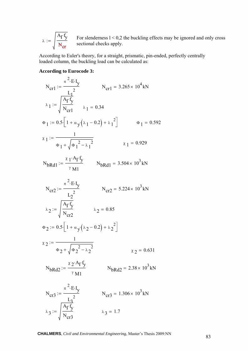
CHALMERS, Civil and Environmental Engineering, Master’s Thesis 2009:NN 83
For slenderness l < 0,2 the buckling effects may be ignored and only cross sectional checks apply.
According to Euler's theory, for a straight, prismatic, pin-ended, perfectly centrally loaded column, the buckling load can be calculated as:
According to Eurocode 3:
λAI fy⋅
Ncr:=
Ncr
Ncr1π
2 E⋅ Iy⋅
L12
:= Ncr1 3.265 104× kN=
λ1AI fy⋅
Ncr1:=
λ1 0.34=
Φ1 0.5 1 αy λ1 0.2−( )⋅+ λ12+⎡
⎣⎤⎦⋅:= Φ1 0.592=
χ 11
Φ1 Φ12
λ12−+
:=χ 1 0.929=
NbRd1χ 1 AI⋅ fy⋅
γ M1:= NbRd1 3.504 103× kN=
Ncr2π
2 E⋅ Iy⋅
L22
:= Ncr2 5.224 103× kN=
λ2AI fy⋅
Ncr2:= λ2 0.85=
Φ2 0.5 1 αy λ2 0.2−( )⋅+ λ22+⎡
⎣⎤⎦⋅:=
χ 21
Φ2 Φ22
λ22−+
:=
χ 2 0.631=
NbRd2χ 2 AI⋅ fy⋅
γ M1:= NbRd2 2.38 103× kN=
Ncr3π
2 E⋅ Iy⋅
L32
:= Ncr3 1.306 103× kN=
λ3AI fy⋅
Ncr3:= λ3 1.7=

CHALMERS, Civil and Environmental Engineering, Master’s Thesis 2009:NN 84
According to Polish Code:
Buckling curve b => n=1,6:
Φ3 0.5 1 αy λ3 0.2−( )⋅+ λ32+⎡
⎣⎤⎦⋅:= Φ3 2.312=
χ 31
Φ3 Φ32
λ32−+
:=
χ 3 0.258=
NbRd3χ 3 AI⋅ fy⋅
γ M1:= NbRd3 972.653 kN=
λPN1 1.15AI fy⋅
Ncr1⋅:=
λPN1 0.391=
φ 1 1 λPN12 1.6⋅+⎛
⎝⎞⎠
1−1.6
:= φ 1 0.97=
NPN1 φ 1 AI⋅ fy⋅:= NPN1 3.66 103× kN=
λPN2 1.15AI fy⋅
Ncr2⋅:=
λPN2 0.977=
φ 2 1 λPN22 1.6⋅+⎛
⎝⎞⎠
1−1.6
:= Φ2 1.02=
NPN2 φ 2 AI⋅ fy⋅:= NPN2 2.502 103× kN=
λPN3 1.15AI fy⋅
Ncr3⋅:= λPN3 1.955=
φ 3 1 λPN32 1.6⋅+⎛
⎝⎞⎠
1−1.6
:= φ 3 0.244=
NPN3 φ 3 AI⋅ fy⋅:= NPN3 921.492 kN=

CHALMERS, Civil and Environmental Engineering, Master’s Thesis 2009:NN 85
SUMMARY OF THE RESULTS:
The design buckling resistance of a compression column of length L1:
The design buckling resistance of a compression column of length L2:
The design buckling resistance of a compression column of length L2:
The value of critical force obtained from buckling analysis performed using ABAQUS:
NbRd1 3.504 103× kN=
NbRd2 2.38 103× kN=
NbRd3 972.653kN=
Ncr1 3.265 104× kN= Pcr2m 30048 kN⋅:=
Ncr2 5.224 103× kN= Pcr5m 5152 kN⋅:=
Ncr3 1.306 103× kN= Pcr10m 1301.3 kN⋅:=

CHALMERS, Civil and Environmental Engineering, Master’s Thesis 2009:NN 86
Simple case 2 - Beam-column
The design buckling resistance moment of a laterally unrestrained beam:
< 1
Buckling curve for HEA300:
< 2
Lateral torsional buckling curve for a Rolled I-section, taken from Table 6.4 from EC3 => curve a
An imperfection factor for lateral torsional buckling curve taken from Table 6.3 EC3:
For buckling curve a, from Table 5.1 from EC3, initial local bow imperfections are equal:
=
For slenderness λLT< 0,4 lateral torsional buckling effects may be ignored and only cross sectional checks apply.
Calculation of elastic critical moment, according to Galambos (1988)
The warping constant:
MbRd χ LT Wx⋅fy
γ M1⋅:= χ LT
χ LT1
ΦLT ΦLT2
λLT2−+
:=ΦLT
Φ 0.5 1 αLT λLT 0.2−( )⋅+ λLT2+⎡
⎣⎤⎦⋅:= αLT
hbf
0.967=
αLT 0.21:=
1350
e01a0.5L1300
:=e0L
e01a 3.333 mm=
e02a0.5L2300
:=e02a 8.333mm=
e03a0.5L3300
:= e03a 16.667mm=
λLTWx fy⋅
Mcr:=
Mcr
CwIy hw
2⋅
4:=

CHALMERS, Civil and Environmental Engineering, Master’s Thesis 2009:NN 87
The pure torsional constant:
First method proposed in Eurocode3:
J2bf tf
3⋅ hw tw3⋅+
3:=
W1π
L1
E Cw⋅
G J⋅:=
Mcr1π
L1E Iy⋅ G⋅ J⋅ 1 W1
2+⎛⎝
⎞⎠⋅⋅:=
W2π
L2
E Cw⋅
G J⋅:= Mcr2
π
L2E Iy⋅ G⋅ J⋅ 1 W2
2+⎛⎝
⎞⎠⋅⋅:=
W3π
L3
E Cw⋅
G J⋅:= Mcr3
π
L3E Iy⋅ G⋅ J⋅ 1 W3
2+⎛⎝
⎞⎠⋅⋅:=
Mcr1 4.459 103× kN m⋅= McrFEM2m 4596.9 kN⋅ m⋅:=
Mcr2 850.024kN m⋅= McrFEM5m 878.46 kN⋅ m⋅:=
McrFEM10m 310.28 kN⋅ m⋅:=Mcr3 304.664 kN m⋅=
λLT1Wx fy⋅
Mcr1:= λLT2
Wx fy⋅
Mcr2:= λLT3
Wx fy⋅
Mcr3:=
λLT1 0.308= λLT2 0.706= λLT3 1.179=
ΦLT1 0.5 1 αLT λLT1 0.2−( )⋅+ λLT12+⎡
⎣⎤⎦⋅:=
ΦLT2 0.5 1 αLT λLT2 0.2−( )⋅+ λLT22+⎡
⎣⎤⎦⋅:=
ΦLT3 0.5 1 αLT λLT3 0.2−( )⋅+ λLT32+⎡
⎣⎤⎦⋅:=
ΦLT1 0.559= ΦLT2 0.802= ΦLT3 1.297=

CHALMERS, Civil and Environmental Engineering, Master’s Thesis 2009:NN 88
< 1
< 1
< 1
The design buckling resistance moment of a laterally unrestrained beam for lengths L1, L2 and L3:
Second method proposed in Eurocode3:
curve b
χ LT11
ΦLT1 ΦLT12
λLT12−+
:=χ LT1 0.976=
χ LT21
ΦLT2 ΦLT22
λLT22−+
:=χ LT2 0.845=
χ LT31
ΦLT3 ΦLT32
λLT32−+
:=χ LT3 0.544=
MbRd1 χ LT1 Wx⋅fy
γ M1⋅:=
MbRd1 412.85 kN m⋅=
MbRd2 χ LT2 Wx⋅fy
γ M1⋅:=
MbRd2 357.628 kN m⋅=
MbRd3 χ LT3 Wx⋅fy
γ M1⋅:= MbRd3 230.071kN m⋅=
λLT1Wx fy⋅
Mcr1:= λLT2
Wx fy⋅
Mcr2:= λLT3
Wx fy⋅
Mcr3:=
λLT1 0.308= λLT2 0.706= λLT3 1.179=
αLT2 0.34:= β 0.75:=
ΦLT1 0.5 1 αLT2 λLT1 0.4−( )⋅+ β λLT12⋅+⎡
⎣⎤⎦⋅:=
ΦLT2 0.5 1 αLT2 λLT2 0.4−( )⋅+ β λLT22⋅+⎡
⎣⎤⎦⋅:=
ΦLT3 0.5 1 αLT2 λLT3 0.4−( )⋅+ β λLT32⋅+⎡
⎣⎤⎦⋅:=

CHALMERS, Civil and Environmental Engineering, Master’s Thesis 2009:NN 89
< 1
< 1
< 1
The design buckling resistance moment of a laterally unrestrained beam:
For buckling curve b, from Table 5.1 from EC3, initial bow imperfections are equal to:
=
ΦLT1 0.52= ΦLT2 0.739= ΦLT3 1.153=
χ LTβ11
ΦLT1 ΦLT12
β λLT12⋅−+
:=χ LTβ1 1.035=
χ LTβ1 1:=χ LTβ2
1
ΦLT2 ΦLT22
β λLT22⋅−+
:=χ LTβ2 0.867=
χ LTβ31
ΦLT3 ΦLT32
β λLT32⋅−+
:=χ LTβ3 0.592=
1
λLT32
0.72=
MbRd1β χ LTβ1 Wx⋅fy
γ M1⋅:=
MbRd1β 423.175kN m⋅=
MbRd2β χ LTβ2 Wx⋅fy
γ M1⋅:=
MbRd2β 366.825kN m⋅=
MbRd3β χ LTβ3 Wx⋅fy
γ M1⋅:= MbRd3β 250.391kN m⋅=
e01a0.5L1250
:=e01a 4 mm=
1250
e02a0.5L2250
:=e0L
e02a 10 mm=
e03a0.5L3250
:= e03a 20 mm=

CHALMERS, Civil and Environmental Engineering, Master’s Thesis 2009:NN 90

CHALMERS, Civil and Environmental Engineering, Master’s Thesis 2009:NN 91
Appendix B
Parametric studies of the I-beam with corrugated web Evaluation of the elastic critical moment

CHALMERS, Civil and Environmental Engineering, Master’s Thesis 2009:NN 92

CHALMERS, Civil and Environmental Engineering, Master’s Thesis 2009:NN 93
Parametric studies of the I-beam with corrugated web
Web thickness:
Web depth:
Corrugation properties :
tw1 2 mm⋅:=tw2 3 mm⋅:= tw 3 mm⋅:=tw3 4 mm⋅:=
hw1 400 mm⋅:=hw2 600 mm⋅:= hw 600 mm⋅:=
hw3 800 mm⋅:=tf 14 mm⋅:=bf 230 mm⋅:=
E 210 GPa⋅:=ν 0.3:=fy 355 MPa⋅:=
GplaneE
2 1 ν+( )⋅:=
Gplane 80.769 GPa=
a 140 mm⋅:=b 50 mm⋅:=
dmax 25 mm⋅:=
L1 10 m⋅:=
c1 b2 2dmax( )2+:=
c1 70.711mm=

CHALMERS, Civil and Environmental Engineering, Master’s Thesis 2009:NN 94
Section properties: The second moment of inertia about the strong axis (x-axis) for different depths:
The second moment of inertia about the weak axis (y-axis):
The shear modulus:
The pure torsional constant for different depths:
The pure torsional constant for different web thicknesses:
Ixco1bf tf⋅ hw1
2
2:= Ixco1 2.576 108× mm4=
Ixco2bf tf⋅ hw2
2
2:= Ixco2 5.796 108× mm4=
Ixco3bf tf⋅ hw3
2
2:= Ixco3 1.03 109× mm4=
Ixcobf tf⋅ hw
2
2:=
Iycotf bf
3
6:= Iyco 2.839 107× mm4=
GcoGplane a b+( )⋅
a c1+:= Gco 72.83GPa=
Jcoh12bf tf
3⋅ hw1 tw3⋅+
3:= Jcoh1 4.243 105× mm4=
Jcoh22bf tf
3⋅ hw2 tw3⋅+
3:= Jcoh2 4.261 105× mm4=
Jcoh32bf tf
3⋅ hw3 tw3⋅+
3:= Jcoh3 4.279 105× mm4=
Jcoh Jcoh2:=
Jcot12bf tf
3⋅ hw tw13⋅+
3:= Jcot1 4.223 105× mm4=
Jcot22bf tf
3⋅ hw tw23⋅+
3:= Jcot2 4.261 105× mm4=
Jcot32bf tf
3⋅ hw tw33⋅+
3:= Jcot3 4.335 105× mm4=

CHALMERS, Civil and Environmental Engineering, Master’s Thesis 2009:NN 95
Calculations for the plane web:
Jco112bf tf
3⋅ hw1 tw13⋅+
3:= Jco21
2bf tf3⋅ hw1 tw2
3⋅+
3:= Jco31
2bf tf3⋅ hw1 tw3
3⋅+
3:=
Jco122bf tf
3⋅ hw2 tw13⋅+
3:= Jco22
2bf tf3⋅ hw2 tw2
3⋅+
3:= Jco32
2bf tf3⋅ hw2 tw3
3⋅+
3:=
Jco332bf tf
3⋅ hw3 tw33⋅+
3:=Jco23
2bf tf3⋅ hw3 tw2
3⋅+
3:=Jco13
2bf tf3⋅ hw3 tw1
3⋅+
3:=
Cwflat1bf
3 tf⋅ hw12⋅
24:= Cwflat2
bf3 tf⋅ hw2
2⋅
24:= Cwflat3
bf3 tf⋅ hw3
2⋅
24:=
Cwflat2 2.555 1012× mm6= Cwflat3 4.542 1012× mm6=Cwflat1 1.136 1012× mm6=
W11π
L1
E Cwflat1⋅
Gplane Jco11⋅:=
Mocrflat11π
L1E Iy⋅ Gplane⋅ Jco11⋅ 1 W11
2+⎛⎝
⎞⎠⋅⋅:=
Mocrflat11 184.108kN m⋅=
W12π
L1
E Cwflat2⋅
Gplane Jco12⋅:=
Mocrflat12π
L1E Iy⋅ Gplane⋅ Jco12⋅ 1 W12
2+⎛⎝
⎞⎠⋅⋅:=
Mocrflat12 226.346kN m⋅=
W13π
L1
E Cwflat3⋅
Gplane Jco13⋅:=
Mocrflat13π
L1E Iy⋅ Gplane⋅ Jco13⋅ 1 W13
2+⎛⎝
⎞⎠⋅⋅:=
W21π
L1
E Cwflat1⋅
Gplane Jco21⋅:=
Mocrflat21π
L1E Iy⋅ Gplane⋅ Jco21⋅ 1 W21
2+⎛⎝
⎞⎠⋅⋅:=

CHALMERS, Civil and Environmental Engineering, Master’s Thesis 2009:NN 96
Method proposed by Lindner:
The warping constant is derived for the I-beam with corrugated web. The torsional constant is the same in case of a plane web and in case of corrugated web.
W22π
L1
E Cwflat2⋅
Gplane Jco22⋅:=
Mocrflat22π
L1E Iy⋅ Gplane⋅ Jco22⋅ 1 W22
2+⎛⎝
⎞⎠⋅⋅:=
W23π
L1
E Cwflat3⋅
Gplane Jco23⋅:=
Mocrflat23π
L1E Iy⋅ Gplane⋅ Jco23⋅ 1 W23
2+⎛⎝
⎞⎠⋅⋅:=
W31π
L1
E Cwflat1⋅
Gplane Jco31⋅:=
Mocrflat31π
L1E Iy⋅ Gplane⋅ Jco31⋅ 1 W31
2+⎛⎝
⎞⎠⋅⋅:=
W32π
L1
E Cwflat2⋅
Gplane Jco32⋅:=
Mocrflat32π
L1E Iy⋅ Gplane⋅ Jco32⋅ 1 W32
2+⎛⎝
⎞⎠⋅⋅:=
W33π
L1
E Cwflat3⋅
Gplane Jco33⋅:=
Mocrflat33π
L1E Iy⋅ Gplane⋅ Jco33⋅ 1 W33
2+⎛⎝
⎞⎠⋅⋅:=
ux11hw1
2 Gplane⋅ a⋅ tw1⋅
hw12 a b+( )3⋅ Ixco1 Iyco+( )⋅
600 a2⋅ E⋅ Ixco1⋅ Iyco⋅+:=
cw112 dmax⋅( )2 hw1
2⋅
8 ux11⋅ a b+( )⋅:=
CL11 Cwflat1cw11 L1
2⋅
E π2⋅
+:= CL11 2.568 1012× mm6=

CHALMERS, Civil and Environmental Engineering, Master’s Thesis 2009:NN 97
WL11π
L1
E CL11⋅
Gplane Jco11⋅:=
MocrL11π
L1E Iyco⋅ Gplane⋅ Jco11⋅ 1 WL11
2+⎛⎝
⎞⎠⋅⋅:=
MocrL11 226.651 kN m⋅=
ux12hw2
2 Gplane⋅ a⋅ tw1⋅
hw22 a b+( )3⋅ Ixco2 Iyco+( )⋅
600 a2⋅ E⋅ Ixco2⋅ Iyco⋅+:=
cw122 dmax⋅( )2 hw2
2⋅
8 ux12⋅ a b+( )⋅:=
CL12 Cwflat2cw12 L1
2⋅
E π2⋅
+:= CL12 4.703 1012× mm6=
WL12π
L1
E CL12⋅
Gplane Jco12⋅:=
MocrL12π
L1E Iyco⋅ Gplane⋅ Jco12⋅ 1 WL12
2+⎛⎝
⎞⎠⋅⋅:=
MocrL12 278.251kN m⋅=
ux13hw3
2 Gplane⋅ a⋅ tw1⋅
hw32 a b+( )3⋅ Ixco3 Iyco+( )⋅
600 a2⋅ E⋅ Ixco3⋅ Iyco⋅+:=
cw132 dmax⋅( )2 hw3
2⋅
8 ux13⋅ a b+( )⋅:=
CL13 Cwflat3cw13 L1
2⋅
E π2⋅
+:= CL13 7.403 1012× mm6=
WL13π
L1
E CL13⋅
Gplane Jco13⋅:=
MocrL13π
L1E Iyco⋅ Gplane⋅ Jco13⋅ 1 WL13
2+⎛⎝
⎞⎠⋅⋅:=
MocrL13 332.243 kN m⋅=
ux21hw1
2 Gplane⋅ a⋅ tw2⋅
hw12 a b+( )3⋅ Ixco1 Iyco+( )⋅
600 a2⋅ E⋅ Ixco1⋅ Iyco⋅+:=

CHALMERS, Civil and Environmental Engineering, Master’s Thesis 2009:NN 98
cw212 dmax⋅( )2 hw1
2⋅
8 ux21⋅ a b+( )⋅:=
CL21 Cwflat1cw21 L1
2⋅
E π2⋅
+:= CL21 3.283 1012× mm6=
WL21π
L1
E CL21⋅
Gplane Jco21⋅:=
MocrL21π
L1E Iyco⋅ Gplane⋅ Jco21⋅ 1 WL21
2+⎛⎝
⎞⎠⋅⋅:=
MocrL21 245.363 kN m⋅=
ux22hw2
2 Gplane⋅ a⋅ tw2⋅
hw22 a b+( )3⋅ Ixco2 Iyco+( )⋅
600 a2⋅ E⋅ Ixco2⋅ Iyco⋅+:=
cw222 dmax⋅( )2 hw2
2⋅
8 ux22⋅ a b+( )⋅:=
CL22 Cwflat2cw22 L1
2⋅
E π2⋅
+:= CL22 5.772 1012× mm6=
WL22π
L1
E CL22⋅
Gplane Jco22⋅:=
MocrL22π
L1E Iyco⋅ Gplane⋅ Jco22⋅ 1 WL22
2+⎛⎝
⎞⎠⋅⋅:=
MocrL22 301.073 kN m⋅=
ux23hw3
2 Gplane⋅ a⋅ tw2⋅
hw32 a b+( )3⋅ Ixco3 Iyco+( )⋅
600 a2⋅ E⋅ Ixco3⋅ Iyco⋅+:=
cw232 dmax⋅( )2 hw3
2⋅
8 ux23⋅ a b+( )⋅:=
CL23 Cwflat3cw23 L1
2⋅
E π2⋅
+:= CL23 8.826 1012× mm6=
WL23π
L1
E CL23⋅
Gplane Jco23⋅:=

CHALMERS, Civil and Environmental Engineering, Master’s Thesis 2009:NN 99
MocrL23π
L1E Iyco⋅ Gplane⋅ Jco23⋅ 1 WL23
2+⎛⎝
⎞⎠⋅⋅:=
MocrL23 357.739kN m⋅=
ux31hw1
2 Gplane⋅ a⋅ tw3⋅
hw12 a b+( )3⋅ Ixco1 Iyco+( )⋅
600 a2⋅ E⋅ Ixco1⋅ Iyco⋅+:=
cw312 dmax⋅( )2 hw1
2⋅
8 ux31⋅ a b+( )⋅:=
CL31 Cwflat1cw31 L1
2⋅
E π2⋅
+:= CL11 2.568 1012× mm6=
WL31π
L1
E CL31⋅
Gplane Jco31⋅:=
MocrL31π
L1E Iyco⋅ Gplane⋅ Jco31⋅ 1 WL31
2+⎛⎝
⎞⎠⋅⋅:=
MocrL31 262.93 kN m⋅=
ux32hw2
2 Gplane⋅ a⋅ tw3⋅
hw22 a b+( )3⋅ Ixco2 Iyco+( )⋅
600 a2⋅ E⋅ Ixco2⋅ Iyco⋅+:=
cw322 dmax⋅( )2 hw2
2⋅
8 ux32⋅ a b+( )⋅:=
CL32 Cwflat2cw32 L1
2⋅
E π2⋅
+:= CL12 4.703 1012× mm6=
WL32π
L1
E CL32⋅
Gplane Jco32⋅:=
MocrL32π
L1E Iyco⋅ Gplane⋅ Jco32⋅ 1 WL32
2+⎛⎝
⎞⎠⋅⋅:=
MocrL32 322.493 kN m⋅=
ux33hw3
2 Gplane⋅ a⋅ tw3⋅
hw32 a b+( )3⋅ Ixco3 Iyco+( )⋅
600 a2⋅ E⋅ Ixco3⋅ Iyco⋅+:=

CHALMERS, Civil and Environmental Engineering, Master’s Thesis 2009:NN 100
The method proposed by Moon et al.:
Average corrugation depth:
Evaluation of the normalized unit warping at point i:
a ) for different depths
For h.w = h.w1
cw332 dmax⋅( )2 hw3
2⋅
8 ux33⋅ a b+( )⋅:=
CL33 Cwflat3cw33 L1
2⋅
E π2⋅
+:= CL33 1.024 1013× mm6=
WL33π
L1
E CL33⋅
Gplane Jco33⋅:=
MocrL33π
L1E Iyco⋅ Gplane⋅ Jco33⋅ 1 WL33
2+⎛⎝
⎞⎠⋅⋅:=
MocrL33 381.752 kN m⋅=
davg2 a⋅ b+( ) dmax⋅
2 a b+( )⋅:= davg 21.711mm=
Wnh112 bf
2⋅ hw1 tf⋅ bf hw12⋅ tw⋅+
8 bf⋅ tf⋅ 4 hw1⋅ tw⋅+:= Wnh11 2.3 104× mm2=
Wnh122 bf
2⋅ hw1 tf⋅ bf hw12⋅ tw⋅+
8 bf⋅ tf⋅ 4 hw1⋅ tw⋅+
bf4
davg2
−⎛⎜⎝
⎞⎟⎠
hw1⋅−:= Wnh12 4.342 103× mm2=
Wnh132 bf
2⋅ hw1 tf⋅ bf hw12⋅ tw⋅+
8 bf⋅ tf⋅ 4 hw1⋅ tw⋅+
bf4
davg2
+⎛⎜⎝
⎞⎟⎠
hw1⋅−:= Wnh13 4.342− 103× mm2=
Wnh142 bf
2⋅ hw1 tf⋅ bf hw12⋅ tw⋅+
8 bf⋅ tf⋅ 4 hw1⋅ tw⋅+12
hw1⋅ bf⋅−:= Wnh14 2.3− 104× mm2=
Wnh15 Wnh14:= Wnh15 2.3− 104× mm2=
Wnh16 Wnh11:= Wnh16 2.3 104× mm2=

CHALMERS, Civil and Environmental Engineering, Master’s Thesis 2009:NN 101
For h.w = h.w2
For h.w = h.w3
Wnh212 bf
2⋅ hw2 tf⋅ bf hw22⋅ tw⋅+
8 bf⋅ tf⋅ 4 hw2⋅ tw⋅+:= Wnh21 3.45 104× mm2=
Wnh222 bf
2⋅ hw2 tf⋅ bf hw22⋅ tw⋅+
8 bf⋅ tf⋅ 4 hw2⋅ tw⋅+
bf4
davg2
−⎛⎜⎝
⎞⎟⎠
hw2⋅−:= Wnh22 6.513 103× mm2=
Wnh232 bf
2⋅ hw2 tf⋅ bf hw22⋅ tw⋅+
8 bf⋅ tf⋅ 4 hw2⋅ tw⋅+
bf4
davg2
+⎛⎜⎝
⎞⎟⎠
hw2⋅−:= Wnh23 6.513− 103× mm2=
Wnh242 bf
2⋅ hw2 tf⋅ bf hw22⋅ tw⋅+
8 bf⋅ tf⋅ 4 hw2⋅ tw⋅+12
hw2⋅ bf⋅−:= Wnh24 3.45− 104× mm2=
Wnh25 Wnh24:= Wnh25 3.45− 104× mm2=
Wnh26 Wnh21:= Wnh26 3.45 104× mm2=
Wnh312 bf
2⋅ hw3 tf⋅ bf hw32⋅ tw⋅+
8 bf⋅ tf⋅ 4 hw3⋅ tw⋅+:= Wnh31 4.6 104× mm2=
Wnh322 bf
2⋅ hw3 tf⋅ bf hw32⋅ tw⋅+
8 bf⋅ tf⋅ 4 hw3⋅ tw⋅+
bf4
davg2
−⎛⎜⎝
⎞⎟⎠
hw3⋅−:= Wnh32 8.684 103× mm2=
Wnh332 bf
2⋅ hw3 tf⋅ bf hw32⋅ tw⋅+
8 bf⋅ tf⋅ 4 hw3⋅ tw⋅+
bf4
davg2
+⎛⎜⎝
⎞⎟⎠
hw3⋅−:= Wnh33 8.684− 103× mm2=
Wnh342 bf
2⋅ hw3 tf⋅ bf hw32⋅ tw⋅+
8 bf⋅ tf⋅ 4 hw3⋅ tw⋅+12
hw3⋅ bf⋅−:= Wnh34 4.6− 104× mm2=
Wnh35 Wnh34:= Wnh35 4.6− 104× mm2=
Wnh36 Wnh31:= Wnh36 4.6 104× mm2=

CHALMERS, Civil and Environmental Engineering, Master’s Thesis 2009:NN 102
b) for different web thicknesses
For t.w = t.w1
For t.w = t.w2
Wnt112 bf
2⋅ hw tf⋅ bf hw2⋅ tw1⋅+
8 bf⋅ tf⋅ 4 hw⋅ tw1⋅+:= Wnt11 3.45 104× mm2=
Wnt122 bf
2⋅ hw tf⋅ bf hw2⋅ tw1⋅+
8 bf⋅ tf⋅ 4 hw⋅ tw1⋅+
bf4
davg2
−⎛⎜⎝
⎞⎟⎠
hw⋅−:= Wnt12 6.513 103× mm2=
Wnt132 bf
2⋅ hw tf⋅ bf hw2⋅ tw1⋅+
8 bf⋅ tf⋅ 4 hw⋅ tw1⋅+
bf4
davg2
+⎛⎜⎝
⎞⎟⎠
hw⋅−:= Wnt13 6.513− 103× mm2=
Wnt142 bf
2⋅ hw tf⋅ bf hw2⋅ tw1⋅+
8 bf⋅ tf⋅ 4 hw⋅ tw1⋅+12
hw⋅ bf⋅−:= Wnt14 3.45− 104× mm2=
Wnt15 Wnt14:= Wnt15 3.45− 104× mm2=
Wnt16 Wnt11:= Wnt16 3.45 104× mm2=
Wnt212 bf
2⋅ hw tf⋅ bf hw2⋅ tw2⋅+
8 bf⋅ tf⋅ 4 hw⋅ tw2⋅+:= Wnt21 3.45 104× mm2=
Wnt222 bf
2⋅ hw tf⋅ bf hw2⋅ tw2⋅+
8 bf⋅ tf⋅ 4 hw⋅ tw2⋅+
bf4
davg2
−⎛⎜⎝
⎞⎟⎠
hw⋅−:= Wnt22 6.513 103× mm2=
Wnt232 bf
2⋅ hw tf⋅ bf hw2⋅ tw2⋅+
8 bf⋅ tf⋅ 4 hw⋅ tw2⋅+
bf4
davg2
+⎛⎜⎝
⎞⎟⎠
hw⋅−:= Wnt23 6.513− 103× mm2=
Wnt242 bf
2⋅ hw tf⋅ bf hw2⋅ tw2⋅+
8 bf⋅ tf⋅ 4 hw⋅ tw2⋅+12
hw⋅ bf⋅−:= Wnt24 3.45− 104× mm2=
Wnt25 Wnt24:= Wnt25 3.45− 104× mm2=
Wnt26 Wnt21:= Wnt26 3.45 104× mm2=

CHALMERS, Civil and Environmental Engineering, Master’s Thesis 2009:NN 103
For t.w = t.w3
Determination of the warping constant for different web thicknesses and depths
Wnt312 bf
2⋅ hw tf⋅ bf hw2⋅ tw3⋅+
8 bf⋅ tf⋅ 4 hw⋅ tw3⋅+:= Wnt31 3.45 104× mm2=
Wnt322 bf
2⋅ hw tf⋅ bf hw2⋅ tw3⋅+
8 bf⋅ tf⋅ 4 hw⋅ tw3⋅+
bf4
davg2
−⎛⎜⎝
⎞⎟⎠
hw⋅−:= Wnt32 6.513 103× mm2=
Wnt332 bf
2⋅ hw tf⋅ bf hw2⋅ tw3⋅+
8 bf⋅ tf⋅ 4 hw⋅ tw3⋅+
bf4
davg2
+⎛⎜⎝
⎞⎟⎠
hw⋅−:= Wnt33 6.513− 103× mm2=
Wnt342 bf
2⋅ hw tf⋅ bf hw2⋅ tw3⋅+
8 bf⋅ tf⋅ 4 hw⋅ tw3⋅+12
hw⋅ bf⋅−:= Wnt34 3.45− 104× mm2=
Wnt35 Wnt34:= Wnt35 3.45− 104× mm2=
Wnt36 Wnt31:= Wnt36 3.45 104× mm2=
Cwco1113
Wnh112 Wnh11 Wnh12⋅+ Wnh12
2+⎛⎝
⎞⎠ tf⋅
bf2
davg−⎛⎜⎝
⎞⎟⎠
⋅
Wnh152 Wnh12 Wnh15⋅+ Wnh12
2+⎛⎝
⎞⎠ tf⋅
bf2
davg+⎛⎜⎝
⎞⎟⎠
⋅+
...
Wnh122 Wnh12 Wnh13⋅+ Wnh13
2+⎛⎝
⎞⎠ tw1⋅ hw1⋅+
...
Wnh132 Wnh14 Wnh13⋅+ Wnh14
2+⎛⎝
⎞⎠ tf⋅
bf2
davg−⎛⎜⎝
⎞⎟⎠
⋅+
...
Wnh162 Wnh13 Wnh16⋅+ Wnh13
2+⎛⎝
⎞⎠ tf⋅
bf2
davg+⎛⎜⎝
⎞⎟⎠
⋅+
...
⎡⎢⎢⎢⎢⎢⎢⎢⎢⎢⎢⎢⎣
⎤⎥⎥⎥⎥⎥⎥⎥⎥⎥⎥⎥⎦
⋅:=
Cwco11 1.141 1012× mm6=

CHALMERS, Civil and Environmental Engineering, Master’s Thesis 2009:NN 104
Cwco1213
Wnh212 Wnh21 Wnh22⋅+ Wnh22
2+⎛⎝
⎞⎠ tf⋅
bf2
davg−⎛⎜⎝
⎞⎟⎠
⋅
Wnh252 Wnh22 Wnh25⋅+ Wnh22
2+⎛⎝
⎞⎠ tf⋅
bf2
davg+⎛⎜⎝
⎞⎟⎠
⋅+
...
Wnh222 Wnh22 Wnh23⋅+ Wnh23
2+⎛⎝
⎞⎠ tw1⋅ hw2⋅+
...
Wnh232 Wnh24 Wnh23⋅+ Wnh24
2+⎛⎝
⎞⎠ tf⋅
bf2
davg−⎛⎜⎝
⎞⎟⎠
⋅+
...
Wnh262 Wnh23 Wnh26⋅+ Wnh23
2+⎛⎝
⎞⎠ tf⋅
bf2
davg+⎛⎜⎝
⎞⎟⎠
⋅+
...
⎡⎢⎢⎢⎢⎢⎢⎢⎢⎢⎢⎢⎣
⎤⎥⎥⎥⎥⎥⎥⎥⎥⎥⎥⎥⎦
⋅:=
Cwco12 2.572 1012× mm6=
Cwco1313
Wnh312 Wnh31 Wnh32⋅+ Wnh32
2+⎛⎝
⎞⎠ tf⋅
bf2
davg−⎛⎜⎝
⎞⎟⎠
⋅
Wnh352 Wnh32 Wnh35⋅+ Wnh32
2+⎛⎝
⎞⎠ tf⋅
bf2
davg+⎛⎜⎝
⎞⎟⎠
⋅+
...
Wnh322 Wnh32 Wnh33⋅+ Wnh33
2+⎛⎝
⎞⎠ tw1⋅ hw3⋅+
...
Wnh332 Wnh34 Wnh33⋅+ Wnh34
2+⎛⎝
⎞⎠ tf⋅
bf2
davg−⎛⎜⎝
⎞⎟⎠
⋅+
...
Wnh362 Wnh33 Wnh36⋅+ Wnh33
2+⎛⎝
⎞⎠ tf⋅
bf2
davg+⎛⎜⎝
⎞⎟⎠
⋅+
...
⎡⎢⎢⎢⎢⎢⎢⎢⎢⎢⎢⎢⎣
⎤⎥⎥⎥⎥⎥⎥⎥⎥⎥⎥⎥⎦
⋅:=
Cwco13 4.583 1012× mm6=
Cwco2113
Wnh112 Wnh11 Wnh12⋅+ Wnh12
2+⎛⎝
⎞⎠ tf⋅
bf2
davg−⎛⎜⎝
⎞⎟⎠
⋅
Wnh152 Wnh12 Wnh15⋅+ Wnh12
2+⎛⎝
⎞⎠ tf⋅
bf2
davg+⎛⎜⎝
⎞⎟⎠
⋅+
...
Wnh122 Wnh12 Wnh13⋅+ Wnh13
2+⎛⎝
⎞⎠ tw2⋅ hw1⋅+
...
Wnh132 Wnh14 Wnh13⋅+ Wnh14
2+⎛⎝
⎞⎠ tf⋅
bf2
davg−⎛⎜⎝
⎞⎟⎠
⋅+
...
Wnh162 Wnh13 Wnh16⋅+ Wnh13
2+⎛⎝
⎞⎠ tf⋅
bf2
davg+⎛⎜⎝
⎞⎟⎠
⋅+
...
⎡⎢⎢⎢⎢⎢⎢⎢⎢⎢⎢⎢⎣
⎤⎥⎥⎥⎥⎥⎥⎥⎥⎥⎥⎥⎦
⋅:=
Cwco21 1.143 1012× mm6=

CHALMERS, Civil and Environmental Engineering, Master’s Thesis 2009:NN 105
Cwco2213
Wnh212 Wnh21 Wnh22⋅+ Wnh22
2+⎛⎝
⎞⎠ tf⋅
bf2
davg−⎛⎜⎝
⎞⎟⎠
⋅
Wnh252 Wnh22 Wnh25⋅+ Wnh22
2+⎛⎝
⎞⎠ tf⋅
bf2
davg+⎛⎜⎝
⎞⎟⎠
⋅+
...
Wnh222 Wnh22 Wnh23⋅+ Wnh23
2+⎛⎝
⎞⎠ tw2⋅ hw2⋅+
...
Wnh232 Wnh24 Wnh23⋅+ Wnh24
2+⎛⎝
⎞⎠ tf⋅
bf2
davg−⎛⎜⎝
⎞⎟⎠
⋅+
...
Wnh262 Wnh23 Wnh26⋅+ Wnh23
2+⎛⎝
⎞⎠ tf⋅
bf2
davg+⎛⎜⎝
⎞⎟⎠
⋅+
...
⎡⎢⎢⎢⎢⎢⎢⎢⎢⎢⎢⎢⎣
⎤⎥⎥⎥⎥⎥⎥⎥⎥⎥⎥⎥⎦
⋅:=
Cwco22 2.581 1012× mm6=
Cwco2313
Wnh312 Wnh31 Wnh32⋅+ Wnh32
2+⎛⎝
⎞⎠ tf⋅
bf2
davg−⎛⎜⎝
⎞⎟⎠
⋅
Wnh352 Wnh32 Wnh35⋅+ Wnh32
2+⎛⎝
⎞⎠ tf⋅
bf2
davg+⎛⎜⎝
⎞⎟⎠
⋅+
...
Wnh322 Wnh32 Wnh33⋅+ Wnh33
2+⎛⎝
⎞⎠ tw2⋅ hw3⋅+
...
Wnh332 Wnh34 Wnh33⋅+ Wnh34
2+⎛⎝
⎞⎠ tf⋅
bf2
davg−⎛⎜⎝
⎞⎟⎠
⋅+
...
Wnh362 Wnh33 Wnh36⋅+ Wnh33
2+⎛⎝
⎞⎠ tf⋅
bf2
davg+⎛⎜⎝
⎞⎟⎠
⋅+
...
⎡⎢⎢⎢⎢⎢⎢⎢⎢⎢⎢⎢⎣
⎤⎥⎥⎥⎥⎥⎥⎥⎥⎥⎥⎥⎦
⋅:=
Cwco23 4.603 1012× mm6=
Cwco3113
Wnh112 Wnh11 Wnh12⋅+ Wnh12
2+⎛⎝
⎞⎠ tf⋅
bf2
davg−⎛⎜⎝
⎞⎟⎠
⋅
Wnh152 Wnh12 Wnh15⋅+ Wnh12
2+⎛⎝
⎞⎠ tf⋅
bf2
davg+⎛⎜⎝
⎞⎟⎠
⋅+
...
Wnh122 Wnh12 Wnh13⋅+ Wnh13
2+⎛⎝
⎞⎠ tw3⋅ hw1⋅+
...
Wnh132 Wnh14 Wnh13⋅+ Wnh14
2+⎛⎝
⎞⎠ tf⋅
bf2
davg−⎛⎜⎝
⎞⎟⎠
⋅+
...
Wnh162 Wnh13 Wnh16⋅+ Wnh13
2+⎛⎝
⎞⎠ tf⋅
bf2
davg+⎛⎜⎝
⎞⎟⎠
⋅+
...
⎡⎢⎢⎢⎢⎢⎢⎢⎢⎢⎢⎢⎣
⎤⎥⎥⎥⎥⎥⎥⎥⎥⎥⎥⎥⎦
⋅:=
Cwco31 1.146 1012× mm6=

CHALMERS, Civil and Environmental Engineering, Master’s Thesis 2009:NN 106
Elastic critical moment for the I-girder with corrugated web:
Cwco3213
Wnh212 Wnh21 Wnh22⋅+ Wnh22
2+⎛⎝
⎞⎠ tf⋅
bf2
davg−⎛⎜⎝
⎞⎟⎠
⋅
Wnh252 Wnh22 Wnh25⋅+ Wnh22
2+⎛⎝
⎞⎠ tf⋅
bf2
davg+⎛⎜⎝
⎞⎟⎠
⋅+
...
Wnh222 Wnh22 Wnh23⋅+ Wnh23
2+⎛⎝
⎞⎠ tw3⋅ hw2⋅+
...
Wnh232 Wnh24 Wnh23⋅+ Wnh24
2+⎛⎝
⎞⎠ tf⋅
bf2
davg−⎛⎜⎝
⎞⎟⎠
⋅+
...
Wnh262 Wnh23 Wnh26⋅+ Wnh23
2+⎛⎝
⎞⎠ tf⋅
bf2
davg+⎛⎜⎝
⎞⎟⎠
⋅+
...
⎡⎢⎢⎢⎢⎢⎢⎢⎢⎢⎢⎢⎣
⎤⎥⎥⎥⎥⎥⎥⎥⎥⎥⎥⎥⎦
⋅:=
Cwco32 2.589 1012× mm6=
Cwco3313
Wnh312 Wnh31 Wnh32⋅+ Wnh32
2+⎛⎝
⎞⎠ tf⋅
bf2
davg−⎛⎜⎝
⎞⎟⎠
⋅
Wnh352 Wnh32 Wnh35⋅+ Wnh32
2+⎛⎝
⎞⎠ tf⋅
bf2
davg+⎛⎜⎝
⎞⎟⎠
⋅+
...
Wnh322 Wnh32 Wnh33⋅+ Wnh33
2+⎛⎝
⎞⎠ tw3⋅ hw3⋅+
...
Wnh332 Wnh34 Wnh33⋅+ Wnh34
2+⎛⎝
⎞⎠ tf⋅
bf2
davg−⎛⎜⎝
⎞⎟⎠
⋅+
...
Wnh362 Wnh33 Wnh36⋅+ Wnh33
2+⎛⎝
⎞⎠ tf⋅
bf2
davg+⎛⎜⎝
⎞⎟⎠
⋅+
...
⎡⎢⎢⎢⎢⎢⎢⎢⎢⎢⎢⎢⎣
⎤⎥⎥⎥⎥⎥⎥⎥⎥⎥⎥⎥⎦
⋅:=
Cwco33 4.623 1012× mm6=
Wco11π
L1
E Cwco11⋅
Gco Jco11⋅:= Wco11 0.877=
Mocr11π
L1E Iyco⋅ Gco⋅ Jco11⋅ 1 Wco11
2+⎛⎝
⎞⎠⋅⋅:=
Mocr11 178.848 kN m⋅=
Wco12π
L1
E Cwco12⋅
Gco Jco12⋅:= Wco12 1.316=
Mocr12π
L1E Iyco⋅ Gco⋅ Jco12⋅ 1 Wco12
2+⎛⎝
⎞⎠⋅⋅:=
Mocr12 222.411kN m⋅=

CHALMERS, Civil and Environmental Engineering, Master’s Thesis 2009:NN 107
Wco13π
L1
E Cwco13⋅
Gco Jco13⋅:= Wco13 1.756=
Mocr13π
L1E Iyco⋅ Gco⋅ Jco13⋅ 1 Wco13
2+⎛⎝
⎞⎠⋅⋅:=
Mocr13 272.045 kN m⋅=
Wco21π
L1
E Cwco21⋅
Gco Jco21⋅:= Wco21 0.876=
Mocr21π
L1E Iyco⋅ Gco⋅ Jco21⋅ 1 Wco21
2+⎛⎝
⎞⎠⋅⋅:=
Mocr21 179.237 kN m⋅=
Wco22π
L1
E Cwco22⋅
Gco Jco22⋅:= Wco22 1.313=
Mocr22π
L1E Iyco⋅ Gco⋅ Jco22⋅ 1 Wco22
2+⎛⎝
⎞⎠⋅⋅:=
Mocr22 223.009 kN m⋅=
Wco23π
L1
E Cwco23⋅
Gco Jco23⋅:= Wco23 1.749=
Mocr23π
L1E Iyco⋅ Gco⋅ Jco23⋅ 1 Wco23
2+⎛⎝
⎞⎠⋅⋅:=
Mocr23 272.894 kN m⋅=
Wco31π
L1
E Cwco31⋅
Gco Jco31⋅:= Wco31 0.871=
Mocr31π
L1E Iyco⋅ Gco⋅ Jco31⋅ 1 Wco31
2+⎛⎝
⎞⎠⋅⋅:=
Mocr31 179.911 kN m⋅=

CHALMERS, Civil and Environmental Engineering, Master’s Thesis 2009:NN 108
Ultimate moment for the I-beam with corrugated web:
Ultimate moment for the I-beam with plane web:
Wco32π
L1
E Cwco32⋅
Gco Jco32⋅:= Wco32 1.304=
Mocr32π
L1E Iyco⋅ Gco⋅ Jco32⋅ 1 Wco32
2+⎛⎝
⎞⎠⋅⋅:=
Mocr32 223.95 kN m⋅=
Wco33π
L1
E Cwco33⋅
Gco Jco33⋅:= Wco33 1.733=
Mocr33π
L1E Iyco⋅ Gco⋅ Jco33⋅ 1 Wco33
2+⎛⎝
⎞⎠⋅⋅:=
Mocr33 274.115kN m⋅=
Multcoh1Ixco1 fy⋅
0.5 hw1⋅ tf+:= Multcoh1 427.327kN m⋅=
Multcoh2Ixco2 fy⋅
0.5 hw2⋅ tf+:= Multcoh2 655.28kN m⋅=
Multcoh3Ixco3 fy⋅
0.5 hw3⋅ tf+:= Multcoh3 883.556kN m⋅=
Multh1Ixco1 fy⋅
0.5 hw1⋅ tf+:= Multh1 427.327 kN m⋅=
Multh2Ixco2 fy⋅
0.5 hw2⋅ tf+:= Multh2 655.28kN m⋅=
Multh3Ixco3 fy⋅
0.5 hw3⋅ tf+:= Multh3 883.556kN m⋅=

CHALMERS, Civil and Environmental Engineering, Master’s Thesis 2009:NN 109
Summary of the results:
tw2tw1Mocrflat11 184.108kN m⋅= Mocrflat21 184.435kN m⋅=
hw1hw1 MocrL11 226.651 kN m⋅= MocrL21 245.363 kN m⋅=
Mocr11 178.848kN m⋅= Mocr21 179.237kN m⋅=
tw1 tw2Mocrflat12 226.346 kN m⋅= Mocrflat22 226.744kN m⋅=
hw2hw2 MocrL12 278.251 kN m⋅= MocrL22 301.073 kN m⋅=Mocr12 222.411kN m⋅= Mocr22 223.009 kN m⋅=
tw1 tw2
Mocrflat13 274.761 kN m⋅= Mocrflat23 275.199 kN m⋅=
MocrL13 332.243kN m⋅= hw3 MocrL23 357.739kN m⋅=hw3Mocr13 272.045 kN m⋅= Mocr23 272.894 kN m⋅=
tw3
Mocrflat31 185.069 kN m⋅=
MocrL31 262.93kN m⋅=hw1Mocr31 179.911kN m⋅=
tw3Mocrflat32 227.519 kN m⋅=
MocrL32 322.493kN m⋅=hw2Mocr32 223.95 kN m⋅=
tw3Mocrflat33 276.049kN m⋅=
hw3 MocrL33 381.752 kN m⋅=
Mocr33 274.115kN m⋅=

CHALMERS, Civil and Environmental Engineering, Master’s Thesis 2009:NN 110

CHALMERS, Civil and Environmental Engineering, Master’s Thesis 2009:NN 111
Appendix C Figures and results from Finite Element Analyses of the frames
with corrugated and plane webs

CHALMERS, Civil and Environmental Engineering, Master’s Thesis 2009:NN 112

CHALMERS, Civil and Environmental Engineering, Master’s Thesis 2009:NN 113
In this Appendix the results of additional Finite Element Analyses presenting lateral-torsional behaviour of the frames with corrugated and plane webs have been collected.
The models which have been described in this Section are:
- the case of the frame without any lateral restraints, with the plane plate in the corner 6mm thick,
- the case of the frame with additional restraint only on the inner flange of the column,
- the case of the frame with additional restraint only on the outer flange of the rafter,
- the case of the frame with additional restraint only on the inner flange of the rafter,
These cases correspond both for the frame with corrugated and with plane webs.
In figures below the areas of yielding have been pictured and out-of plane deflection has been presented.
The results which have been presented in this section have mainly theoretical value. In reality this kind of restraints would not be adopted individually as has been done in these analyses. This investigation is supposed to enable better understanding of the behaviour of the analysed frames.
In Tables C.1 and C.2, in the end of this Appendix, the results from Finite Element Analyses for both frames have been collected.

CHALMERS, Civil and Environmental Engineering, Master’s Thesis 2009:NN 114
For the case of the frame with corrugated webs, with the plane plate in the corner 6mm thick yielding of the first fibres has been observed in the plane plate in the corner. The load level which has been obtained has been equal to 13,85kN/m, which corresponds to the reaction force equal to 152,4kN. The area of yielding for this case has been shown in Figure C.1
Figure C.1 The area of yielding for the frame with corrugated webs without any
lateral restraints for the frame with the thickness of the plate in the corner equal to 6mm.
In this case in-plane deflection in U1 direction has been equal to 24mm. Out-of plane deflection in U3 direction has been equal to maximum 36mm for the inner flange of the rafter, 34mm for the outer flange of the rafter and around 18mm for the inner flange of the column.
The out-of-plane deflection of this model has been illustrated in Figure C.2 below.
Figure C.2 Out-of-plane deflection of the frame with corrugated webs without any
lateral restraints for the frame with the thickness of the plate in the corner equal to 6mm.

CHALMERS, Civil and Environmental Engineering, Master’s Thesis 2009:NN 115
For the analogical case of the frame with plane webs yielding of the first fibres has been observed in the plane plate in the corner and in the stiffener. The load level which has been obtained has been equal to 15,7kN/m, which corresponds to the reaction force equal to 172,6kN. The area of yielding for this case has been shown in Figure C.3
Figure C.3 The area of yielding for the frame with plane webs without any lateral
restraints for the frame with the thickness of the plate in the corner equal to 6mm.
In this case in-plane deflection in U1 direction has been equal to mm. Out-of plane deflection in U3 direction has been equal to maximum 36mm for the inner flange of the rafter, 34mm for the outer flange of the rafter and around 18mm for the inner flange of the column. The out-of-plane deflection of this model has been illustrated in Figure C.4 below.
Figure C.4 Out-of-plane deflection of the frame with plane webs without any lateral
restraints for the frame with the thickness of the plate in the corner equal to 6mm.

CHALMERS, Civil and Environmental Engineering, Master’s Thesis 2009:NN 116
For the case of the frame with corrugated webs, with one additional lateral restraint in the inner flange of the column yielding of the first fibres has been observed in the lower flange of the rafter and in the inner flange of the column. The load level which has been obtained has been equal to 20,9kN/m, which corresponds to the reaction force equal to 229,8kN. The area of yielding has been shown in Figure C.5 below.
Figure C.5 The area of yielding for the frame with corrugated webs with one lateral
restraint on the inner flange of the column. In this case in-plane deflection in U1 direction has been equal to 24mm. Out-of plane deflection in U3 direction has been equal to maximum 22mm for the inner flange of the rafter, 57mm for the outer flange of the rafter and less than 1mm for the inner flange of the column. The out-of-plane deflection of this model has been illustrated in Figure C.6 below.
Figure C.6 Out-of-plane deflection of the frame with corrugated webs with one lateral
restraint on the inner flange of the column.
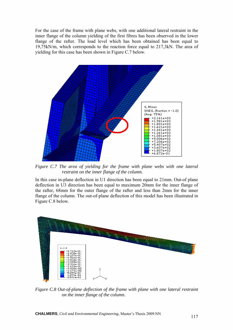
CHALMERS, Civil and Environmental Engineering, Master’s Thesis 2009:NN 117
For the case of the frame with plane webs, with one additional lateral restraint in the inner flange of the column yielding of the first fibres has been observed in the lower flange of the rafter. The load level which has been obtained has been equal to 19,75kN/m, which corresponds to the reaction force equal to 217,3kN. The area of yielding for this case has been shown in Figure C.7 below.
Figure C.7 The area of yielding for the frame with plane webs with one lateral
restraint on the inner flange of the column. In this case in-plane deflection in U1 direction has been equal to 21mm. Out-of plane deflection in U3 direction has been equal to maximum 20mm for the inner flange of the rafter, 68mm for the outer flange of the rafter and less than 2mm for the inner flange of the column. The out-of-plane deflection of this model has been illustrated in Figure C.8 below.
Figure C.8 Out-of-plane deflection of the frame with plane with one lateral restraint
on the inner flange of the column.
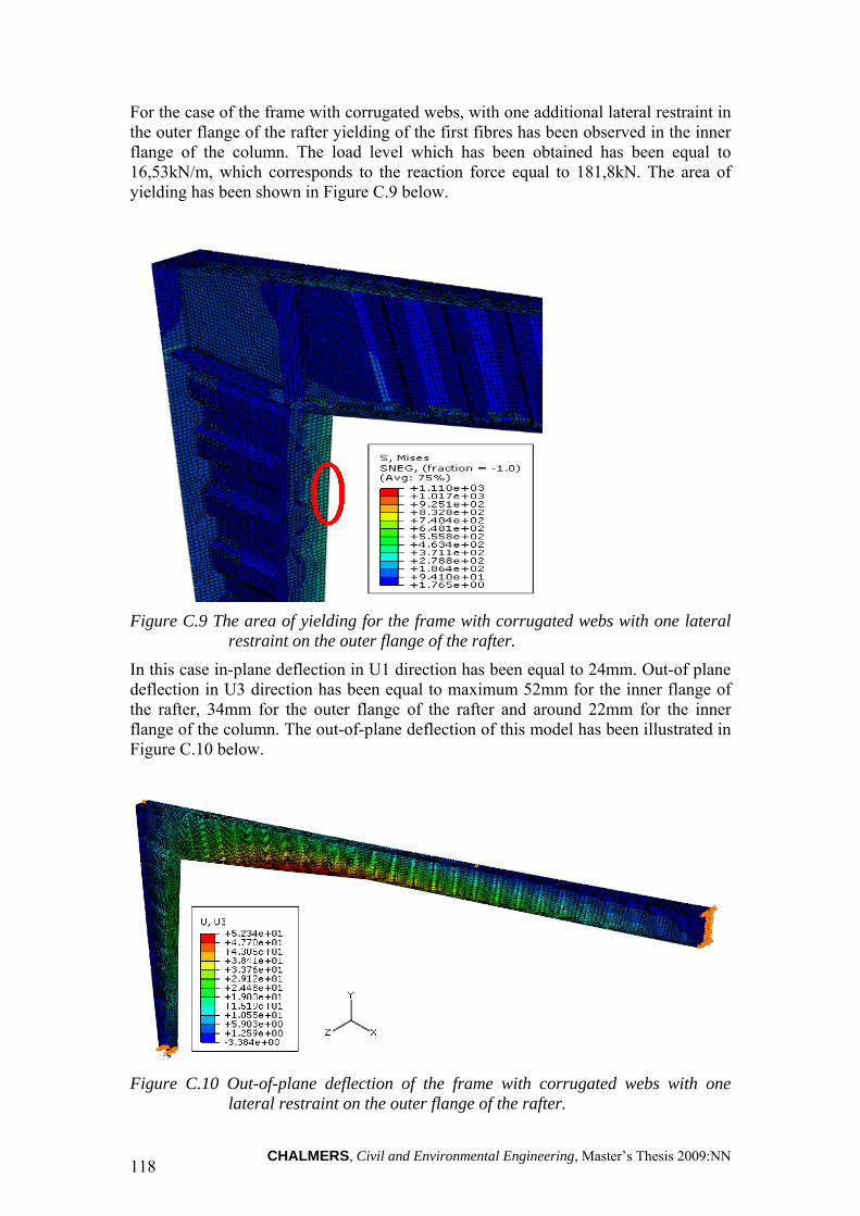
CHALMERS, Civil and Environmental Engineering, Master’s Thesis 2009:NN 118
For the case of the frame with corrugated webs, with one additional lateral restraint in the outer flange of the rafter yielding of the first fibres has been observed in the inner flange of the column. The load level which has been obtained has been equal to 16,53kN/m, which corresponds to the reaction force equal to 181,8kN. The area of yielding has been shown in Figure C.9 below.
Figure C.9 The area of yielding for the frame with corrugated webs with one lateral
restraint on the outer flange of the rafter. In this case in-plane deflection in U1 direction has been equal to 24mm. Out-of plane deflection in U3 direction has been equal to maximum 52mm for the inner flange of the rafter, 34mm for the outer flange of the rafter and around 22mm for the inner flange of the column. The out-of-plane deflection of this model has been illustrated in Figure C.10 below.
Figure C.10 Out-of-plane deflection of the frame with corrugated webs with one
lateral restraint on the outer flange of the rafter.
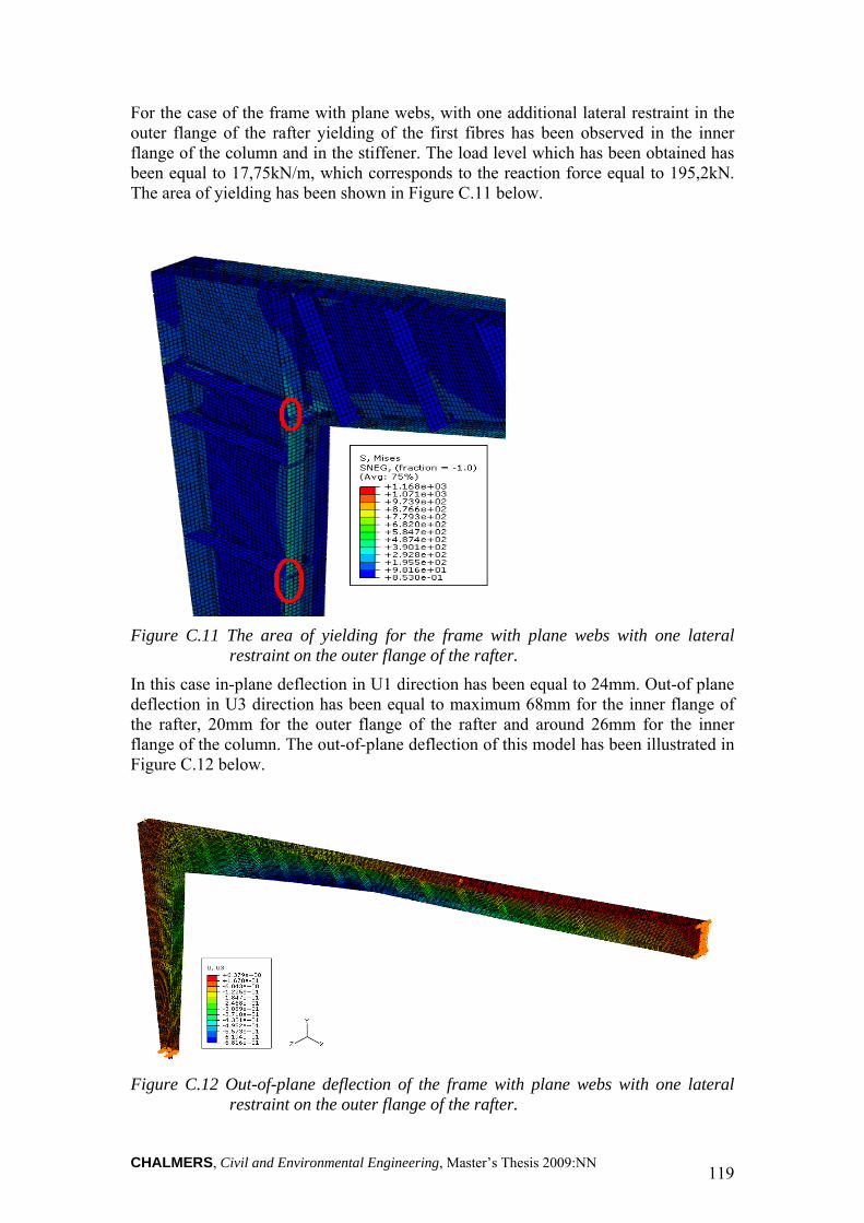
CHALMERS, Civil and Environmental Engineering, Master’s Thesis 2009:NN 119
For the case of the frame with plane webs, with one additional lateral restraint in the outer flange of the rafter yielding of the first fibres has been observed in the inner flange of the column and in the stiffener. The load level which has been obtained has been equal to 17,75kN/m, which corresponds to the reaction force equal to 195,2kN. The area of yielding has been shown in Figure C.11 below.
Figure C.11 The area of yielding for the frame with plane webs with one lateral
restraint on the outer flange of the rafter. In this case in-plane deflection in U1 direction has been equal to 24mm. Out-of plane deflection in U3 direction has been equal to maximum 68mm for the inner flange of the rafter, 20mm for the outer flange of the rafter and around 26mm for the inner flange of the column. The out-of-plane deflection of this model has been illustrated in Figure C.12 below.
Figure C.12 Out-of-plane deflection of the frame with plane webs with one lateral
restraint on the outer flange of the rafter.

CHALMERS, Civil and Environmental Engineering, Master’s Thesis 2009:NN 120
For the case of the frame with corrugated webs, with one additional lateral restraint in the inner flange of the rafter yielding of the first fibres has been observed in the inner flange of the column. The load level which has been obtained has been equal to 19kN/m, which corresponds to the reaction force equal to 209kN. The area of yielding for this case has been shown in Figure C.13 below.
Figure C.13 The area of yielding for the frame with corrugated webs with one lateral
restraint on the inner flange of the rafter. In this case in-plane deflection in U1 direction has been equal to 23mm. Out-of plane deflection in U3 direction has been equal to maximum 8mm for the inner flange of the rafter, 57mm for the outer flange of the rafter and around 9mm for the inner flange of the column. The out-of-plane deflection of this model has been illustrated in Figure C.14 below.
Figure C.14 Out-of-plane deflection of the frame with corrugated webs with one
lateral restraint on the inner flange of the rafter.

CHALMERS, Civil and Environmental Engineering, Master’s Thesis 2009:NN 121
For the last case of the frame with plane webs, with one additional lateral restraint in the inner flange of the rafter yielding of the first fibres has been observed in the inner flange of the column and in the stiffener. The load level which has been obtained has been equal to 18,4kN/m, which corresponds to the reaction force equal to 202,3kN. The area of yielding for this case has been shown in Figure C.15 below.
Figure C.15 The area of yielding for the frame with plane webs with one lateral
restraint on the inner flange of the rafter. In this case in-plane deflection in U1 direction has been equal to 21mm. Out-of plane deflection in U3 direction has been equal to maximum 7mm for the inner flange of the rafter, 69mm for the outer flange of the rafter and around 14mm for the inner flange of the column. The out-of-plane deflection of this model has been illustrated in Figure C.16 below.
Figure C.16 Out-of-plane deflection of the frame with plane webs with one lateral
restraint on the inner flange of the rafter.

CHALMERS, Civil and Environmental Engineering, Master’s Thesis 2009:NN 122
Table C.1 Results from Finite Element Analysis for the frame with corrugated webs.
CORRUGATED Reaction force Load Area of yielding
U1 U3 lower U3 upper U3 column S column S lower Supper [kN] [kN/m] [mm] [mm] [mm] [mm] [MPa] [MPa] [MPa]
no purlins 152,4 13,85 corner+column 24,3 35,7 34,4 18 355 298 207 corner 6mm no purlins 165 15,00 connection 21 36 30 18 363 291 230
corner 8mm 171,8 15,62 column 22 39 32,8 19 358 311 246
column 1side 214,3 19,48 connection 22 18 50 1 334 320 291 229,8 20,89 low. f.+column 24 22 57 1 362 355 326
column 2 sides 217,1 19,74 connection 21,5 12 51 <1 338 344 286 225,4 20,49 low. f.+column 22,5 13 54 <1 355 369 303
one purlin 174,7 15,88 connection 23 49 31 20 340 305 227 181,8 16,53 column 24 52 34 22 356 324 240
one lateral rest. 201,2 18,29 connection 22 9 61 9 341 265 255 209,1 19,01 column 23 8 57 8,5 358 278 285
purlins every 1m 246,8 22,44 lower flange 24 20 <1 <1 330 355 170
purlins every 2m 246,8 22,44 lower flange 24 20 <1 <1 340 355 170
purlins every 3m 246,8 22,44 lower flange 24 20 <1 <1 342 356 170
purlins every 3m+ 216,5 19,68 connection 21 3/1,56 <1 <1 280 232 150
lateral restraint 282,6 25,69 column 27,5 4/-2 <1 <1 362 306 190

CHALMERS, Civil and Environmental Engineering, Master’s Thesis 2009:NN 123
Table C.1 Results from Finite Element Analysis for the frame with plane webs.
PLANE Reaction force Load Area of
yielding U1 U3 lower U3 upper U3 column S column S lower Supper
[kN] [kN/m] [mm] [mm] [mm] [mm] [MPa] [MPa] [MPa] no purlins 161,9 14,72 stiffener 20 40 39 19 329 245 207
corner 6mm 172,6 15,69 corner 22 45 44 22 360 280 235 no purlins 162,8 14,80 stiffener 20 39,5 37 18 305 250 211
corner 8mm 178,6 16,24 column 22 48 44 22 355 293 247
column 1side 207,2 18,84 stiffener 20 19 64 2 230 341 286 213,9 19,45 lower flange 21 20 68 2 238 358 300
column 2 sides 203,1 18,46 lower flange 19 11 67 3 236 355 257
one purlin 178,5 16,23 stiffener 22 58 18 22 307 280 284 195,2 17,75 column 25 68 20 26 359 330 306
one lateral rest. 195,7 17,79 stiffener 20 6 65 13 338 224 271 202,3 18,39 column 21 6,5 69 14 355 232 283
purlins every 1m 232,2 21,11 lower flange 20 21 <1 <1 265 357 155
purlins every 2m 232,2 21,11 lower flange 20 21 <1 <1 263 357 155
purlins every 3m 232,1 21,10 lower flange 20 21 <1 <1 264 357 155
purlins every 3m+ 297,8 27,07 lower flange 26 7,5/2 <1 <1 329 355 190
lateral restraint


![[N. S. Trahair]Flexural-Torsional Buckling of Strorg)](https://img.pdfslide.us/doc/110x75/55cf8e61550346703b919745/n-s-trahairflexural-torsional-buckling-of-strorg.jpg)