Embed Size (px)
Citation preview

Vehicle System DynamicsVol. 50, No. 8, August 2012, 1209–1224
Lateral dynamics of a bicycle with a passive rider model:stability and controllability
A.L. Schwaba*, J.P. Meijaardb and J.D.G. Kooijmana
aLaboratory for Engineering Mechanics, Delft University of Technology, Mekelweg 2, NL 2628 CDDelft, The Netherlands; bMechanical Automation and Mechatronics, Faculty of Engineering
Technology, University of Twente, Enschede, The Netherlands
(Received 18 May 2011; final version received 23 July 2011 )
This paper addresses the influence of a passive rider on the lateral dynamics of a bicycle model and thecontrollability of the bicycle by steer or upper body sideway lean control. In the uncontrolled modelproposed by Whipple in 1899, the rider is assumed to be rigidly connected to the rear frame of thebicycle and there are no hands on the handlebar. Contrarily, in normal bicycling the arms of a rider areconnected to the handlebar and both steering and upper body rotations can be used for control. Fromobservations, two distinct rider postures can be identified. In the first posture, the upper body leansforward with the arms stretched to the handlebar and the upper body twists while steering. In the secondrider posture, the upper body is upright and stays fixed with respect to the rear frame and the arms,hinged at the shoulders and the elbows, exert the control force on the handlebar. Models can be madewhere neither posture adds any degrees of freedom to the original bicycle model. For both postures, theopen loop, or uncontrolled, dynamics of the bicycle–rider system is investigated and compared withthe dynamics of the rigid-rider model by examining the eigenvalues and eigenmotions in the forwardspeed range 0–10 m/s. The addition of the passive rider can dramatically change the eigenvalues andtheir structure. The controllability of the bicycles with passive rider models is investigated with eithersteer torque or upper body lean torque as a control input. Although some forward speeds exist forwhich the bicycle is uncontrollable, these are either considered stable modes or are at very low speeds.From a practical point of view, the bicycle is fully controllable either by steer torque or by upper bodylean, where steer torque control seems much easier than upper body lean.
Keywords: bicycle dynamics; non-holonomic systems; multibody dynamics; human control; modalcontrollability
1. Introduction
The bicycle is an intriguing machine as it is laterally unstable at low speeds and stable, or easyto stabilise, at high speeds. During the last decade a revival in the research on dynamics andcontrol of bicycles has taken place [1–3]. Most studies use the so-called Whipple model [4]of a bicycle. In this model, a hands-free rigid rider is fixed to the rear frame. However, fromexperience it is known that some form of control is required to stabilise the bicycle and followa path. This control is either applied by steering or by performing some set of upper body
*Corresponding author. Email: [email protected]
ISSN 0042-3114 print/ISSN 1744-5159 online© 2012 Taylor & Francishttp://dx.doi.org/10.1080/00423114.2011.610898http://www.tandfonline.com
Dow
nloa
ded
by [
Bib
lioth
eek
TU
Del
ft]
at 1
2:39
01
Sept
embe
r 20
12

1210 A.L. Schwab et al.
Figure 1. Bicycling on a treadmill, two distinct postures: (a) RiderA on the hybrid bicycle with body leaned forwardand stretched arms and (b) Rider A on the city bicycle with an upright body and flexed arms.
motions. The precise control used by the rider is currently under study [5,6]. Here, we focuson two subjects: (i) the contribution of passive body motions to the uncontrolled dynamics ofa bicycle, and (ii) the controllability of these extended models with either steering or upperbody lean as a control input.
From observations [5,6], two distinct rider postures can be identified. In the first posture, theupper body leans forward with stretched arms on the handlebar, see Figure 1(a). For steering,the upper body needs to twist. In the second rider posture, the upper body stays upright andfixed with respect to the rear frame and the arms, hinging at the shoulders and the elbows, areconnected to the handlebar, see Figure 1(b). For both postures, models can be made with thesame number of degrees of freedom as the original Whipple bicycle model. In other words,both rider models just add a mechanism to the original system without any additional degreesof freedom. In order to describe the control by applying a lean torque from the lower body tothe upper body, both posture models are extended with an extra degree of freedom to describethe upper body lean.
Only a few people have investigated the controllability of a bicycle. Nagai [7] used a simplebicycle model in which only the rear frame and rider have mass, the trail is zero and the steerangle and upper body sideway lean angle are kinematic control inputs. He finds one non-zeroforward speed and one condition on the mass distribution which result in uncontrollability forthe system. Seffen et al. [8] investigate controllability for a bicycle model similar to the modelderived by Sharp [9] with steer torque as the control input. They introduce an index, based on[10], which should indicate the difficulty of riding. The index is based on the ratio of the largestand smallest singular values of the controllability matrix. Neither work addresses whether theuncontrollable mode is stable or unstable, although Seffen et al. [8] mention stabilisability. Itcould well be that the uncontrollable or nearly uncontrollable mode is a stable mode of thesystem that is inessential for the desired output and therefore of no concern to the rider. Thispaper tries to resolve that problem by determining the forward speed at which the bicycle isuncontrollable and then identifying whether this corresponds to a stable or unstable mode. Thisapproach results in discrete speeds for which the system is uncontrollable. To investigate thecontrollability by a continuous measure, the concept of modal controllability, as introducedby Hamdan and Nayfeh [11], is applied.
Dow
nloa
ded
by [
Bib
lioth
eek
TU
Del
ft]
at 1
2:39
01
Sept
embe
r 20
12

Vehicle System Dynamics 1211
The paper is organised as follows. First the original bicycle model is presented. Next theextension of this model with a twisting upper body or flexed arms is presented and the stabilityof the lateral motions is compared with that of a rigid rider model in a forward speed range0–10 m/s. Then the models are extended with a degree of freedom for the upper body sidewaylean and the controllability is investigated for the two cases in which either the steer torqueor the upper body lean torque is a control input. The paper ends with some conclusions. Theappendix summarises the data for the bicycle models.
2. Bicycle model
The basic bicycle model used is the so-called Whipple model [4], which recently has beenbenchmarked [2]. The model, see Figure 2, consists of four rigid bodies connected by revolutejoints. The contact between the knife-edged wheels and the flat level surface is modelled byholonomic constraints in the normal direction, prescribing the wheels to touch the surface,and by non-holonomic constraints in the longitudinal and lateral directions, prescribing zerolongitudinal and lateral slips. In this original model, it is assumed that the rider is rigidlyattached to the rear frame and has no hands on the handlebar. The resulting non-holonomicmechanical model has three velocity degrees of freedom: forward speed v, lean rate φ andsteering rate δ.
For the stability analysis of the lateral motions, we consider the linearised equations ofmotion for small perturbations about the upright steady forward motion. These linearisedequations of motion are fully described in [2]. They are expressed in terms of small changes inthe lateral degrees of freedom (the rear frame roll angle, φ, and the steering angle, δ) from theupright straight-ahead configuration (φ, δ) = (0, 0), at a forward speed v, and have the form
Mq + vC1q + [gK0 + v2K2]q = f , (1)
where the time-varying variables are q = [φ, δ]T and the lean and steering torques aref = [Tφ , Tδ]T. The coefficients in this equation are: a constant symmetric mass matrix, M,a damping-like (there is no real damping) matrix, vC1, which is linear in the forward speed v,and a stiffness matrix which is the sum of a constant symmetric part, gK0, and a part, v2K2,which is quadratic in the forward speed. The forces on the right-hand side, f , are the appliedforces which are energetically dual to the degrees of freedom q. In the upright straight-ahead
x
z
wc
ls
QP
F,leehwtnorFR,leehwraeR
Rear frame includingrider Body, B
Front frame (fork andHandlebar), H
Steer axis
Figure 2. The bicycle model: four rigid bodies (rear wheel R, rear frame B, front handlebar assembly H and frontwheel F) connected by three revolute joints (rear hub, steering axis and front hub), together with the coordinatesystem.
Dow
nloa
ded
by [
Bib
lioth
eek
TU
Del
ft]
at 1
2:39
01
Sept
embe
r 20
12

1212 A.L. Schwab et al.
configuration, the linearised equation of motion for the forward motion is decoupled from thelinearised equations of motion of the lateral motions and simply reads v = 0.
Besides the equations of motion, kinematic differential equations for the configurationvariables that are not degrees of freedom have to be added to complete the description. Forthe forward motion, the equations for the rotation angles of the wheels are θR = −v/rR,θF = −v/rF, where θR and θF are the rotation angles of the rear and front wheel and rR
and rF are the corresponding wheel radii. For the lateral motion, the equations for the yaw(heading) angle, ψ , and the lateral displacement of the rear wheel contact point, yP, areψ = (vδ + cδ) cos λs/w and yP = vψ . For the case of the bicycle, these equations can beconsidered as a system in series with the system defined by the equations of motion (1) withq and q as inputs and the configuration variables as outputs. The stability and controllabilityof the two systems can therefore be studied separately.
The entries in the constant coefficient matrices M, C1, K0 and K2 can be calculated from anon-minimal set of 25 bicycle parameters as described in [2]. A procedure for measuring theseparameters for a real bicycle is described in [12], whereas measured values for the bicyclesused in this study are listed in Table A2 of the appendix. Then, with the coefficient matricesthe characteristic equation,
det(Mλ2 + vC1λ + gK0 + v 2K2) = 0, (2)
can be formed and the eigenvalues, λ, can be calculated. In principle, there are up to foureigenmodes, where oscillatory eigenmodes come in pairs. Two are significant and are tra-ditionally called the capsize mode and the weave mode, see Figure 3(a). The capsize modecorresponds to a real eigenvalue with an eigenvector dominated by lean: when unstable, thebicycle follows a spiralling path with increasing curvature until it falls. The weave mode is anoscillatory motion in which the bicycle sways about the heading direction. The third remainingeigenmode is the overall stable castering mode, like in a trailing caster wheel, which corre-sponds to a large negative real eigenvalue with an eigenvector dominated by steering. Theeigenvalues corresponding to the kinematic differential equations are all zero and correspondto changes in the rotation angles of the wheels, a constant yaw angle and a linearly increasinglateral displacement.
0 1 2 3 4 5 6 7 8 9 10-10
-8
-6
-4
-2
0
2
4
6
8
10
vw vcv (m/s)
(a)
Re(l)
Im(l)
[1/s]weave
capsize
caster
0 1 2 3 4 5 6 7 8 9 10-10
-8
-6
-4
-2
0
2
4
6
8
10
vw vcv (m/s)
(b)
Re(l)
Im(l)
[1/s] weave
capsize
caster
Figure 3. Eigenvalues for the lateral motions of a bicycle–rider combination in a forward speed range of0 m/s < v < 10 m/s, (a) with a completely rigid rider and hands-free and (b) with a rider with stretched arms,hands on the handlebar and a yawing upper body according to the model from Figure 4(a). Note that the bicycle ispassively self-stable between the weave speed vw and the capsize speed vc.
Dow
nloa
ded
by [
Bib
lioth
eek
TU
Del
ft]
at 1
2:39
01
Sept
embe
r 20
12
Vehicle System Dynamics 1213
At near-zero speeds, typically 0 m/s < v < 0.5 m/s, there are two pairs of real eigenvalues.Each pair consists of a positive and a negative eigenvalue and corresponds to aninverted-pendulum-like falling of the bicycle. The positive root in each pair corresponds tofalling, whereas the negative root corresponds to a righting motion. For v = 0, these two arerelated by a time reversal of the motion. When speed is increased, two real eigenvalues coa-lesce and then split to form a complex conjugate pair; this is where the oscillatory weavemotion emerges. At first, this motion is unstable, but at v = vw ≈ 4.8 m/s, the weave speed,these eigenvalues cross the imaginary axis at a Hopf bifurcation and this mode becomes sta-ble. At a higher speed, the capsize eigenvalue crosses the origin at a pitchfork bifurcationat v = vc ≈ 7.9 m/s, the capsize speed, and the bicycle becomes mildly unstable. The speedrange for which the uncontrolled bicycle shows asymptotically stable behaviour, with alleigenvalues having negative real parts, is vw < v < vc.
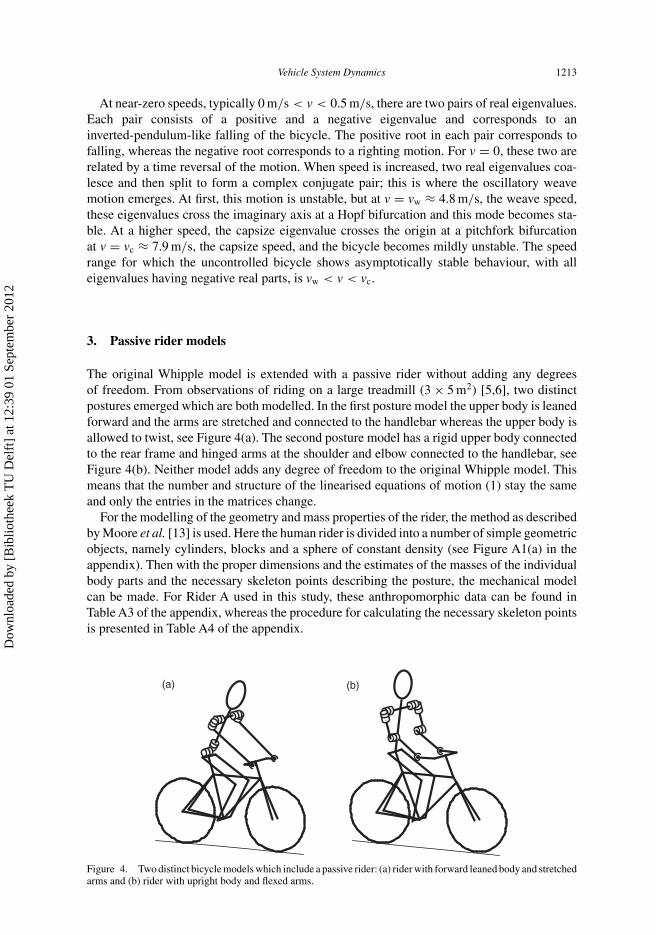
3. Passive rider models
The original Whipple model is extended with a passive rider without adding any degreesof freedom. From observations of riding on a large treadmill (3 × 5 m2) [5,6], two distinctpostures emerged which are both modelled. In the first posture model the upper body is leanedforward and the arms are stretched and connected to the handlebar whereas the upper body isallowed to twist, see Figure 4(a). The second posture model has a rigid upper body connectedto the rear frame and hinged arms at the shoulder and elbow connected to the handlebar, seeFigure 4(b). Neither model adds any degree of freedom to the original Whipple model. Thismeans that the number and structure of the linearised equations of motion (1) stay the sameand only the entries in the matrices change.
For the modelling of the geometry and mass properties of the rider, the method as describedby Moore et al. [13] is used. Here the human rider is divided into a number of simple geometricobjects, namely cylinders, blocks and a sphere of constant density (see Figure A1(a) in theappendix). Then with the proper dimensions and the estimates of the masses of the individualbody parts and the necessary skeleton points describing the posture, the mechanical modelcan be made. For Rider A used in this study, these anthropomorphic data can be found inTable A3 of the appendix, whereas the procedure for calculating the necessary skeleton pointsis presented in Table A4 of the appendix.
(a) (b)
Figure 4. Two distinct bicycle models which include a passive rider: (a) rider with forward leaned body and stretchedarms and (b) rider with upright body and flexed arms.
Dow
nloa
ded
by [
Bib
lioth
eek
TU
Del
ft]
at 1
2:39
01
Sept
embe
r 20
12

1214 A.L. Schwab et al.
The geometric and mass properties of the two bicycles used in this study were obtainedby the procedure described in [12] and the results are presented in Tables A1 and A2 of theappendix.
The complete model of the bicycle with a passive rider was analysed with the multibodydynamics software package SPACAR [14]. This package can handle systems of rigid andflexible bodies connected by various joints in both open and closed kinematic loops, whereparts may have rolling contact [15,16]. The package generates numerically, and solves, fullnon-linear dynamics equations using minimal coordinates (constraints are eliminated). It canalso be used to find the numeric coefficients for the linearised equations of motion based on asemi-analytic linearisation of the non-linear equations. This technique has been used here togenerate the constant coefficient matrices M, C1, K0 and K2 from the linearised equations ofmotion (1), which serve as a basis for generating the eigenvalues of the lateral motions in thedesired forward speed range.
3.1. Forward leaned passive rider
In the model for leaned forward posture, the arms are stretched and the upper and lower armsare modelled as one rigid body each, connected by universal joints to the torso and by balljoints to the handlebar (see Figure 4(a)). The torso is allowed to twist and pitch. Note that in afirst-order approximation, the pitching motion is zero, which follows directly from symmetryarguments. The legs are rigidly attached to the rear frame. The linearised equations of motionare derived as described above and the eigenvalues and eigenmotions of the lateral motionsare calculated in a forward speed range 0–10 m/s. These eigenvalues are shown in Figure 3(b).For comparison, the eigenvalues of a Whipple-like rigid rider model are shown in Figure 3(a).In the rigid rider model we assume the same forward leaned posture but now with no handson the handlebar and the complete rider rigidly attached to the rear frame.
Compared with the rigid rider solutions, there are some small changes in the eigenvalues,but the overall structure is the same. Most noticeable are that the stable speed range goes upand that the frequency of the weave motion goes down. These changes can be explained fromtwo major contributing factors. The first is that the attached passive mechanism of arms andtwisting upper body adds a mass moment of inertia to the steering assembly. This increasesthe diagonal mass term Mδδ of the mass matrix for the steering degree of freedom from 0.28to 0.72 kg m2. The off-diagonal terms increase slightly (10%). The added mass increases theweave speed and decreases the weave frequencies over the considered speed range. The secondfactor is the added stiffness to the steering assembly due to the compressive forces exertedby the hands on the handlebar. This affects several entries in the matrices of the linearisedequations; the most noticeable are the changes in the symmetric static stiffness matrix gK0.The diagonal term for the steering stiffness, gK0δδ , decreases from −6.9 to −9.7 N m/rad andthe off-diagonal terms decrease by 10%. The effects on the eigenvalues are an increased weaveand capsize speed and an overall decrease of weave frequencies, whereas the structure of theeigenvalues with respect to the forward speed remains about the same. It should also be notedthat the more the direction of the stretched arms is parallel to the steer axis, the less the changein the dynamics compared with the rigid rider model is.
3.2. Upright passive rider
In the upright posture, the torso and the legs are rigidly connected to the rear frame. The upperarms are connected to the torso by universal joints and the lower arms are connected to theupper arms by single hinges at the elbows and by ball joints at the handlebar (see Figure 4(b)).
Dow
nloa
ded
by [
Bib
lioth
eek
TU
Del
ft]
at 1
2:39
01
Sept
embe
r 20
12

Vehicle System Dynamics 1215
0 1 2 3 4 5 6 7 8 9 10-10
-8
-6
-4
-2
0
2
4
6
8
10
vw vc
(a)
Re(l)
Im(l)
Re(l)
Im(l)
[1/s] weave
capsize
caster
0 1 2 3 4 5 6 7 8 9 10-10
-8
-6
-4
-2
0
2
4
6
8
10(b)
[1/s]
weave
weave
capsize
caster
v (m/s) v (m/s)
Figure 5. Eigenvalues for the lateral motions of a bicycle–rider combination (a) with a fully rigid rider and hands-freeand (b) with a rider with rigid upper body and flexed arms and hands on the handlebar according to the model fromFigure 4(b).
The linearised equations of motion are derived as described above and the eigenvalues of thelateral motions are computed. These eigenvalues are shown in Figure 5(b). For comparison,the eigenvalues of a Whipple-like rigid rider model are shown in Figure 5(a). In the rigid ridermodel, we assume the same upright posture, but now with no hands on the handlebar and thecomplete rider rigidly attached to the rear frame.
Compared with the rigid rider solutions, there are dramatic changes in the eigenvalues andtheir structure. The stable forward speed range has disappeared completely, because the weavespeed has decreased to zero and the capsize motion is always unstable. Note that the weavemotion is now always stable but gets washed out by the unstable capsize. This dramatic changecan be explained as follows. By adding the hinged arms to the handlebar, a stable pendulum-type of oscillator has been added to the steer assembly. Although this oscillator stabilises theinitially unstable weave motion, it kills the self-stability of the bicycle; the steer-into-the-fallmechanism is made ineffective. The added pendulum mass is most noticeable in the diagonalmass matrix entry related to steering, Mδδ , which increases from 0.25 to 0.46 kg m2. Moredramatic is the change in the constant symmetric stiffness matrix gK0, where the stiffnessrelated to steering, gK0δδ , increases from a negative value, −6.6 N m/rad, to a positive value,2.3 N m/rad, which partly explains the dramatic change in the eigenvalue structure.
4. Controllability
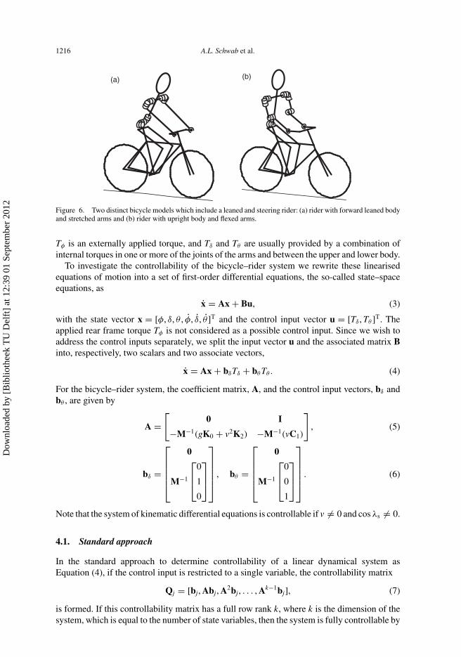
The controllability of the bicycles with passive rider models is investigated where either steertorque or upper body lean torque are considered as a control input. Therefore, both posturemodels will be extended with an extra degree of freedom to describe the upper body lean. Theextended models for both postures are shown in Figure 6. The upper body lean angle θ is madepossible by a hinge between the rear frame and the torso located at the saddle, position number13 in Figure A1(b) of the appendix, with the hinge axis along the lengthwise x-direction.
The structure of the linearised equations of motion remains identical to that of Equation (1),but the number of equations increases from two to three. The three degrees of freedom forthe lateral motion are now the rear frame roll angle, φ, the steer angle, δ, and the upperbody lean angle, θ . The equations are linearised in the upright straight ahead configuration(φ, δ, θ) = (0, 0, 0) at a forward speed v and have the form of Equation (1) where the time-varying variables are now q = [φ, δ, θ ]T and the lean and steering torques are f = [Tφ , Tδ , Tθ ]T.
Dow
nloa
ded
by [
Bib
lioth
eek
TU
Del
ft]
at 1
2:39
01
Sept
embe
r 20
12
1216 A.L. Schwab et al.
(a) (b)
Figure 6. Two distinct bicycle models which include a leaned and steering rider: (a) rider with forward leaned bodyand stretched arms and (b) rider with upright body and flexed arms.
Tφ is an externally applied torque, and Tδ and Tθ are usually provided by a combination ofinternal torques in one or more of the joints of the arms and between the upper and lower body.
To investigate the controllability of the bicycle–rider system we rewrite these linearisedequations of motion into a set of first-order differential equations, the so-called state–spaceequations, as
x = Ax + Bu, (3)
with the state vector x = [φ, δ, θ , φ, δ, θ ]T and the control input vector u = [Tδ , Tθ ]T. Theapplied rear frame torque Tφ is not considered as a possible control input. Since we wish toaddress the control inputs separately, we split the input vector u and the associated matrix Binto, respectively, two scalars and two associate vectors,
x = Ax + bδTδ + bθTθ . (4)
For the bicycle–rider system, the coefficient matrix, A, and the control input vectors, bδ andbθ , are given by
A =[
0 I
−M−1(gK0 + v2K2) −M−1(vC1)
], (5)
bδ =
⎡⎢⎢⎢⎢⎣
0
M−1
⎡⎢⎣
0
1
0
⎤⎥⎦
⎤⎥⎥⎥⎥⎦ , bθ =
⎡⎢⎢⎢⎢⎣
0
M−1
⎡⎢⎣
0
0
1
⎤⎥⎦
⎤⎥⎥⎥⎥⎦ . (6)
Note that the system of kinematic differential equations is controllable if v �= 0 and cos λs �= 0.
4.1. Standard approach
In the standard approach to determine controllability of a linear dynamical system asEquation (4), if the control input is restricted to a single variable, the controllability matrix
Qj = [bj, Abj, A2bj, . . . , Ak−1bj], (7)
is formed. If this controllability matrix has a full row rank k, where k is the dimension of thesystem, which is equal to the number of state variables, then the system is fully controllable by
Dow
nloa
ded
by [
Bib
lioth
eek
TU
Del
ft]
at 1
2:39
01
Sept
embe
r 20
12

Vehicle System Dynamics 1217
Table 1. Forward speed vu at which the hybrid bicycle with the forward leaned rider withstretched arms on the handlebar from Figure 6(a) is uncontrollable by either steer torquecontrol Tδ or upper body lean torque control Tθ together with the corresponding eigenvalueλu and right eigenvector coordinates (φ, δ, θ)u, with rear frame lean angle φ, steer angle δ
and upper body lean angle θ together with the mode description; see also Figure 7 for theeigenvalue plot.
vu (m/s) λu (rad/s) (φ, δ, θ)u (rad) Mode
Steer torque control, Tδ
0.0091 −3.0150 (0.14, 0.56, −0.82) Capsize1.5482 −3.0150 (0.15, 0.69, −0.71) Capsize1.7656 7.8250 (0.15, 0.71, −0.69) Lean14.5588 −7.8250 (0.06, −0.28, 0.96) Caster
Upper body lean torque control, Tθ
0.0067 3.0177 (0.14, 0.56, −0.82) Weave1.5033 −3.0233 (0.15, 0.69, −0.71) Capsize
0 1 2 3 4 5 6 7 8 9 10-10
-8
-6
-4
-2
0
2
4
6
8
10
vw vcv (m/s)
v (m/s)
v (m/s)
(a)
Re(l)
Im(l)
[1/s]
lean1
weave
capsize
caster
lean2
0 1 2 3 4 5 6 7 8 9 1090
60
30
0(b)
b id(°)
b iq(°)
lean1
weave
capsize
casterlean2
0 1 2 3 4 5 6 7 8 9 1090
60
30
0(c)
lean1
weave
capsize caster
lean2
Figure 7. (a) Eigenvalues λ from the linearised stability analysis for the hybrid bicycle with the forward leanedrider with stretched arms on the handlebar from Figure 6(a), where the solid lines correspond to the real part of theeigenvalues and the dashed line corresponds to the imaginary part of the eigenvalues, in the forward speed rangeof 0 m/s < v < 10 m/s, together with forward speeds for which the bicycle is uncontrollable by either steer torque(open circle) or upper body lean torque (black filled circle) alone. (b) Modal controllability βiδ (8) for steer controltorque Tδ for this bicycle model. (c) Modal controllability βiθ (8) for an upper body control lean torque Tθ for thisbicycle model.
input j, j = δ or j = θ , alone. Here, we determine the speeds for which rank deficiency occursby setting the determinant of Qj(v) equal to zero and solving the resulting equation in v. Thesolutions are the forward speeds for which the system is uncontrollable with respect to theconsidered control input, which we call vu. The corresponding eigenvector, v∗
u, spans the nullspace of the transpose of the corresponding controllability matrix, v∗
u ∈ null(QTj (vu)). Since
this is also an eigenvector of the system matrix AT(vu), the corresponding eigenvalue λu canbe found from the definition ATv∗
u = λuv∗u. The corresponding right eigenvector vu satisfies
Avu = λuvu and gives the uncontrollable mode of the system. This procedure has been appliedto the two bicycle–rider models and the results are presented in Table 1 and Figure 7 and inTable 2 and Figure 8.
For the hybrid bicycle with the forward leaned rider with stretched arms on the handlebar,controlled by steer torque control, we find four uncontrollable forward speeds, see Table 1
Dow
nloa
ded
by [
Bib
lioth
eek
TU
Del
ft]
at 1
2:39
01
Sept
embe
r 20
12

1218 A.L. Schwab et al.
Table 2. As Table 1, but now for the city bicycle with an upright rider and flexed arms onthe handlebar from Figure 6(b), see also Figure 8 for the eigenvalue plot.
vu (m/s) λu (rad/s) (φ, δ, θ)u (rad) Mode
Steer torque control, Tδ
0.0133 −2.8980 (0.16, 0.47, −0.87) Caster0.8271 6.5895 (0.14, 0.44, −0.89) Lean11.0177 −2.8980 (0.14, 0.43, −0.89) Caster4.1381 −6.5895 (0.01, −0.26, 0.97) Lean2
Upper body lean torque control, Tθ
0.2695 2.9017 (0.16, 0.46, −0.87) Capsize1.2375 −2.9125 (0.13, 0.42, −0.90) Caster
0 1 2 3 4 5 6 7 8 9 10-10
-8
-6
-4
-2
0
2
4
6
8
10
v (m/s)
v (m/s)
v (m/s)
[1/s]
lean1 weave
capsize
weavecaster
lean2
0 1 2 3 4 5 6 7 8 9 1090
60
30
0
lean1
weave
capsizecaster
lean2
0 1 2 3 4 5 6 7 8 9 1090
60
30
0
lean1
weavecapsizecaster
lean2
(a)(b)
(c)
Re(l)
Im(l)
b id(°)
b iq(°)
Figure 8. (a) Eigenvalues λ from the linearised stability analysis for the city bicycle with an upright rider and flexedarms on the handlebar from Figure 6(b), where the solid lines correspond to the real parts of the eigenvalues and thedashed line corresponds to the imaginary part of the eigenvalues, in the forward speed range of 0 m/s < v < 10 m/s,together with forward speeds for which the bicycle is uncontrollable by either steer torque (open circle) or upper bodylean torque (black filled circle) alone. (b) Modal controllability βiδ (8) for steer control torque Tδ for this bicyclemodel. (c) Modal controllability βiθ (8) for an upper body control lean torque Tθ for this bicycle model.
and Figure 7(a). However, only the one at 1.7656 m/s concerns an unstable mode, an upperbody lean mode. This mode can be stabilised by placing a spring and a damper in parallelbetween the lower and upper body. For a spring stiffness of 100 N m/rad and a dampingcoefficient of 10 N m s/rad, the lean modes become stable and oscillatory, whereas the othermodes change. The uncontrollability shifts to a much lower speed and corresponds to a weavemode. If we consider only upper body lean torque control, then there are two uncontrollableforward speeds, but again only one, now at 0.0067 m/s, concerns an unstable mode. This modeis the forerunner to the oscillatory weave mode, but since the speed is almost zero, this is againof no concern to the practical control of the bicycle. Adding a spring and damper acting inparallel with the control torque has no influence on the controllability. We conclude that thisbicycle–rider configuration is fully controllable by either steer torque control or upper bodylean torque control.
For the city bicycle with an upright rider and flexed arms on the handlebar we first findthat the eigenvalue structure differs considerably from that of the hybrid bicycle with riderconfiguration. Whereas the hybrid bicycle had a stable forward speed range, between 7.4 and8.7 m/s, the city bicycle configuration is always unstable. Although the weave mode is now
Dow
nloa
ded
by [
Bib
lioth
eek
TU
Del
ft]
at 1
2:39
01
Sept
embe
r 20
12

Vehicle System Dynamics 1219
always stable, there is a capsize mode which is always unstable. For steer torque control on thecity bicycle configuration (see Table 2 and Figure 8(a)), we find again four forward speeds forwhich the bicycle is uncontrollable, where only the one at 0.8271 m/s concerns an unstablemode. As with the hybrid bicycle, this is again an upper body lean mode that can be stabilisedby adding a spring and a damper between the lower and the upper body; again, this shiftsthe uncontrollability to a much lower speed for the weave mode. For upper body lean controlwe have two uncontrollable speeds, where only the one at 0.2695 m/s concerns an unstablecapsize mode. But since this is at a very low speed, one can say that, from a practical point ofview, this configuration is also fully controllable by either steer torque control or upper bodylean torque.
4.2. Modal controllability
The standard approach as described above results in a discrete set of velocities for whichthe bicycle is uncontrollable. It does not tell us anything about the ease or difficulty withwhich the bicycle is controlled in the neighbourhood of these speeds at which controllabilityis lost. To investigate that, we will follow a somewhat different approach and look at the modalcontrollability.
A measure for modal controllability has been proposed by Hamdan and Nayfeh [11]. Theymeasure modal controllability by the angle βij between the left eigenvector v∗
i from ATv∗i =
λiv∗i , and the control input vector bj, as in
cos βij = v∗Ti bj
‖v∗i ‖‖bj‖ . (8)
They argue that, if the two vectors are orthogonal, then v∗i is in the left null-space of bj and the
ith eigenmode is uncontrollable from the jth input. If the angle is not a right angle but nearlyso, then again this indicates that the ith eigenmode is not easily controlled from the jth input.This modal controllability is applied to the two bicycle–rider models from Figure 6.
For steer torque control on the hybrid bicycle with the forward leaned rider with stretchedarms on the handlebar, the modal controllability βiδ is shown in Figure 7(b). Note that thevertical scale for the modal controllability angle βij runs from down 90◦ (uncontrollable)to up 0◦ (well controllable). Clearly, the unstable weave mode is well controllable. We alsosee two sharp dips in the capsize mode controllability near the uncontrollable speeds. It isinteresting to see that the uncontrollability is so local, but since this capsize mode is still astable mode, it is of no practical concern. What we call the caster mode shows a broad diparound the uncontrollable forward speed of 4.6 m/s, which seems paradoxical, because weuse steer torque control, but note that there is still some steer amplitude in the correspondingeigenvector (φ, δ, θ)u = (0.06, −0.28, 0.96) (Table 1). As expected, the unstable upper bodylean mode (lean1) is marginally controllable by steer torque control and shows a wide diparound the uncontrollable speed of 1.8 m/s. The modal controllability for upper body leantorque control on this bicycle–rider model is shown in Figure 7(c). Here, we see that themodal controllability of the unstable weave mode is close to 90◦ and therefore hard to controlby lateral upper body motions. The same holds for the capsize mode, with a notable small riseof the modal controllability just above the speed for which the mode in uncontrollable. Thecaster mode also shows marginal controllability. The unstable upper body lean mode (lean1)is well controllable, which we would expect, but its modal controllability levels off at higherspeeds. Note that the modal controllability for the lean torque input is almost the complementof the one for the steer torque input, meaning that the two inputs taken together make thesystem well controllable.
Dow
nloa
ded
by [
Bib
lioth
eek
TU
Del
ft]
at 1
2:39
01
Sept
embe
r 20
12

1220 A.L. Schwab et al.
The modal controllability of the city bicycle with the upright rider and flexed arms on thehandlebar for steer torque control is shown in Figure 8(b). The unstable capsize mode andthe stable weave mode are well controllable. In the stable caster and lean2 modes, we seesharp dips around the uncontrollable speeds and here again the unstable upper body lean ismarginally controllable by this steer torque control. The modal controllability for upper bodylean torque control on this bicycle–rider model is shown in Figure 8(c). The same trends asin the hybrid bicycle are present, meaning that the unstable mode, here the capsize mode, ishard to control by upper body lean motions. It is interesting to see that the overall structure ofthe modal controllability is about the same as in the hybrid bicycle, although the structure ofthe eigenvalues with respect to forward speed is completely different.
We conclude that for both bicycle–rider combinations the controllability of the unstablemodes is very good for steer torque control and marginal for upper body lean motions. Theuncontrollable speeds, which are present, are of no real concern since they are either at stablemodes which are not practically important for the overall desired motion or at very low forwardspeeds for which human control is difficult because of the relatively large positive real partsof the unstable eigenvalues.
5. Conclusions
Adding a passive upper body to the three degrees of freedom Whipple model of an uncontrolledbicycle, without adding any extra degrees of freedom, can change the open-loop dynamicsof the system. In the case of a forward leaned rider with stretched arms and hands on thehandlebar, there is little change. However, an upright rider position with flexed arms and handson the handlebar changes the open-loop dynamics drastically and ruins the self-stability ofthe system.
The unstable modes of both bicycle–rider combinations have very good modal controlla-bility for steer torque control but are marginally controllable by lateral upper body motions.This indicates that most control actions for lateral balance on a bicycle are performed by steercontrol only and not by lateral upper body motions.
Future work is directed towards the comparison of the control effort of the human rider inboth postures.
Acknowledgement
Thanks to Jason Moore for measuring the bicycles and riders during his Fulbright granted year (2008/2009) at TUDelft and thanks to Batavus (Accell Group) for supplying the bicycles.
References
[1] K.J. Åström, R.E. Klein, and A. Lennartsson, Bicycle dynamics and control, IEEE Control Syst. Mag. 25(4)(2005), pp. 26–47.
[2] J.P. Meijaard, J.M. Papadopoulos, A. Ruina, and A.L. Schwab, Linearized dynamics equations for the balanceand steer of a bicycle: a benchmark and review, Proc. Roy. Soc. A 463 (2007), pp. 1955–1982.
[3] R.S. Sharp, On the stability and control of the bicycle, Appl. Mech. Rev. 61 (2008), pp. 060803-1–24.[4] F.J.W. Whipple, The stability of the motion of a bicycle, Quart. J. Pure Appl. Math. 30 (1899), pp. 312–348.[5] J.D.G. Kooijman, J. Moore, and A.L. Schwab, Some observations on human control of a bicycle, in 11th
mini Conference on Vehicle System Dynamics, Identification and Anomalies (VSDIA2008), Budapest, Hungary,I. Zobory, ed., Budapest University of Technology and Economics, 2008, pp. 65–72.
[6] J.K. Moore, J.D.G. Kooijman, and A.L. Schwab, Rider motion identification during normal bicycling by meansof principal component analysis. in MULTIBODY DYNAMICS 2009, ECCOMAS Thematic Conference, 29June–2 July 2009, K. Arczewski, J. Fraczek and M. Wojtyra, eds., Warsaw, Poland, 2009.
Dow
nloa
ded
by [
Bib
lioth
eek
TU
Del
ft]
at 1
2:39
01
Sept
embe
r 20
12

Vehicle System Dynamics 1221
[7] M. Nagai, Analysis of rider and single-track-vehicle system; its application to computer-controlled bicycles,Automatica 19(6) (1983), pp. 737–740.
[8] K.A. Seffen, G.T. Parks, and P.J. Clarkson, Observations on the controllability of motion of two-wheelers, Proc.Inst. Mech. Eng. I J. Syst. Control Eng. 215(2) (2001) pp. 143–156.
[9] R.S. Sharp, The stability and control of motorcycles, J. Mech. Eng. Sci. 13(5) (1971), pp. 316–329.[10] B. Friedland, Controllability index based on conditioning number, J. Dyn. Syst. Meas. Control 97(4) (1975),
pp. 444–445.[11] A.M.A. Hamdan and A.H. Nayfeh, Measures of modal controllability and observability for first- and second-
order linear systems, J. Guidance Control Dyn. 12(3) (1989), pp. 421–428.[12] J.D.G. Kooijman,A.L. Schwab, and J.P. Meijaard, Experimental validation of a model of an uncontrolled bicycle,
Multibody Syst. Dyn. 19 (2008), pp. 115–132.[13] J.K. Moore, M. Hubbard, J.D.G. Kooijman, and A.L. Schwab, A method for estimating physical properties
of a combined bicycle and rider, Proceedings of the ASME 2009 International Design Engineering TechnicalConferences & Computers and Information in Engineering Conference, DETC2009, 30 August–2 September,San Diego, CA, 2009.
[14] J.B. Jonker and J.P. Meijaard, SPACAR - Computer program for dynamic analysis of flexible spatial mechanismsand manipulators, in Multibody Systems Handbook,W. Schiehlen, ed., Springer, Berlin, Germany, 1990, pp. 123–143.
[15] A.L. Schwab and J.P. Meijaard, Dynamics of flexible multibody systems having rolling contact: Application ofthe wheel element to the dynamics of road vehicles. Veh. Syst. Dyn. (Suppl.) 33 (2000), pp. 338–349.
[16] A.L. Schwab and J.P. Meijaard, Dynamics of flexible multibody systems with non-holonomic constraints: A finiteelement approach, Multibody Syst. Dyn. 10(1) (2003), pp. 107–123.
Appendix 1. Measured bicycle and rider data
This appendix summarises the measured geometric and mass data of the bicycles and rider used, measured accordingto [13]. The first bicycle, Figure 1(a), can be characterised as a hybrid bicycle. The second bicycle, Figure 1(b), is astandard Dutch city bicycle (see Figure A1).
Figure A1. (a) Definition of the geometric parameters of the bicycle and (b) rider model with skeleton points,from [13].
Dow
nloa
ded
by [
Bib
lioth
eek
TU
Del
ft]
at 1
2:39
01
Sept
embe
r 20
12
1222 A.L. Schwab et al.
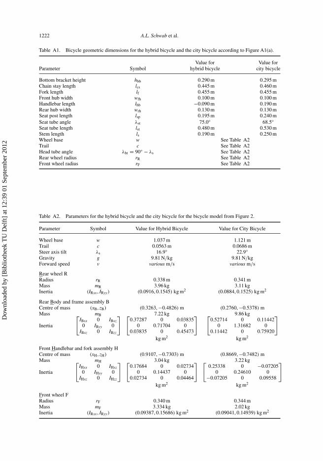
Table A1. Bicycle geometric dimensions for the hybrid bicycle and the city bicycle according to Figure A1(a).
Value for Value forParameter Symbol hybrid bicycle city bicycle
Bottom bracket height hbb 0.290 m 0.295 mChain stay length lcs 0.445 m 0.460 mFork length lf 0.455 m 0.455 mFront hub width wfh 0.100 m 0.100 mHandlebar length lhb −0.090 m 0.190 mRear hub width wrh 0.130 m 0.130 mSeat post length lsp 0.195 m 0.240 mSeat tube angle λst 75.0◦ 68.5◦Seat tube length lst 0.480 m 0.530 mStem length ls 0.190 m 0.250 mWheel base w See Table A2Trail c See Table A2Head tube angle λht = 90◦ − λs See Table A2Rear wheel radius rR See Table A2Front wheel radius rF See Table A2
Table A2. Parameters for the hybrid bicycle and the city bicycle for the bicycle model from Figure 2.
Parameter Symbol Value for Hybrid Bicycle Value for City Bicycle
Wheel base w 1.037 m 1.121 mTrail c 0.0563 m 0.0686 mSteer axis tilt λs 16.9◦ 22.9◦Gravity g 9.81 N/kg 9.81 N/kgForward speed v various m/s various m/s
Rear wheel RRadius rR 0.338 m 0.341 mMass mR 3.96 kg 3.11 kgInertia (IRxx , IRyy) (0.0916, 0.1545) kg m2 (0.0884, 0.1525) kg m2
Rear Body and frame assembly BCentre of mass (xB, zB) (0.3263, −0.4826) m (0.2760, −0.5378) mMass mB 7.22 kg 9.86 kg
Inertia
⎡⎣IBxx 0 IBxz
0 IByy 0IBxz 0 IBzz
⎤⎦
⎡⎣0.37287 0 0.03835
0 0.71704 00.03835 0 0.45473
⎤⎦
⎡⎣0.52714 0 0.11442
0 1.31682 00.11442 0 0.75920
⎤⎦
kg m2 kg m2
Front Handlebar and fork assembly HCentre of mass (xH, zH) (0.9107, −0.7303) m (0.8669, −0.7482) mMass mH 3.04 kg 3.22 kg
Inertia
⎡⎣IHxx 0 IHxz
0 IHyy 0IHxz 0 IHzz
⎤⎦
⎡⎣0.17684 0 0.02734
0 0.14437 00.02734 0 0.04464
⎤⎦
⎡⎣ 0.25338 0 −0.07205
0 0.24610 0−0.07205 0 0.09558
⎤⎦
kg m2 kg m2
Front wheel FRadius rF 0.340 m 0.344 mMass mF 3.334 kg 2.02 kgInertia (IRxx , IRyy) (0.09387, 0.15686) kg m2 (0.09041, 0.14939) kg m2
Dow
nloa
ded
by [
Bib
lioth
eek
TU
Del
ft]
at 1
2:39
01
Sept
embe
r 20
12

Vehicle System Dynamics 1223
Table A3. Anthropomorphic data for Rider A according to Figure A1(b).
Parameter Symbol Rider A
Chest circumference cch 0.94 mForward lean angle λfl 63.9◦ (on hybrid bicycle)
82.9◦ (on city bicycle)Head circumference ch 0.58 mHip joint to hip joint lhh 0.26 mLower arm circumference cla 0.23 mLower arm length lla 0.33 mLower leg circumference cll 0.38 mLower leg length lll 0.46 mShoulder to shoulder lss 0.44 mTorso length lto 0.48 mUpper arm circumference cua 0.30 mUpper arm length lua 0.28 mUpper leg circumference cul 0.50 mUpper leg length lul 0.46 mRider mass mBr 72.0 kgHead mass mh 0.068 mBrLower arm mass mla 0.022 mBrLower leg mass mll 0.061 mBrTorso mass mto 0.510 mBrUpper arm mass mua 0.028 mBrUpper leg mass mul 0.100 mBr
Table A4. Skeleton points code according to Figure A1.
%% Matlab code for Skeleton Grid Points see Figure A1a%% Adapted Table 10 from MooreHubbardKooijmanSchwab2009r1 = [0 0 0];r2 = [0 0 -rR];r3 = r2 + [0 wrh/2 0];r4 = r2 + [0 -wrh/2 0];r5 = [sqrt(lcsˆ2-(rR-hbb)ˆ2) 0 -hbb];r6 = [w 0 0];r7 = r6 + [0 0 -rF];r8 = r7 + [0 wfh/2 0];r9 = r7 + [0 -wfh/2 0];r10 = r5 + [-lst*cos(last) 0 -lst*sin(last)];% calculate f0f0 = rF*cos(laht)-c*sin(laht);r11 = r7 + [-f0*sin(laht)-sqrt(lfˆ2-f0ˆ2)*cos(laht)…0 f0*cos(laht)-sqrt(lfˆ2-f0ˆ2)*sin(laht)];
r12 = [r11(1)-(r11(3)-r10(3))/tan(laht) 0 r10(3)];r13 = r10 + [-lsp*cos(last) 0 -lsp*sin(last)];% determine mid knee angle and mid knee positiona1 = atan2((r5(1)-r13(1)),(r5(3)-r13(3)));l1 = sqrt((r5(1)-r13(1))ˆ2+(r5(3)-r13(3))ˆ2);a2 = acos((l1ˆ2+lulˆ2-lllˆ2)/(2*l1*lul));%r14 = r13 + [lul*sin(a1+a2) 0 lul*cos(a1+a2)];r15 = r13 + [lto*cos(lafl) 0 -lto*sin(lafl)];r16 = r12 + [-ls*cos(laht) 0 -ls*sin(laht)];r17 = r16 + [0 lss/2 0];r18 = r16 + [0 -lss/2 0];r19 = r17 + [-lhb 0 0];r20 = r18 + [-lhb 0 0];r21 = r15 + [0 lss/2 0];r22 = r15 + [0 -lss/2 0];% determine left elbow positiona1 = atan2((r19(1)-r21(1)),(r19(3)-r21(3)));
Dow
nloa
ded
by [
Bib
lioth
eek
TU
Del
ft]
at 1
2:39
01
Sept
embe
r 20
12

1224 A.L. Schwab et al.
Table A4. Continued
l1 = sqrt((r19(1)-r21(1))ˆ2+(r19(3)-r21(3))ˆ2);a2 = acos((l1ˆ2+luaˆ2-llaˆ2)/(2*l1*lua));%r23 = r21 + [lua*sin(a1-a2) 0 lua*cos(a1-a2)];r24 = r23 + [0 -lss 0];r25 = r15 + [ch/(2*pi)*cos(lafl) 0 -ch/(2*pi)*sin(lafl)];r26 = r5 + [0 lhh/2 0];r27 = r5 + [0 -lhh/2 0];r28 = r14 + [0 lhh/2 0];r29 = r14 + [0 -lhh/2 0];r30 = r13 + [0 lhh/2 0];r31 = r13 + [0 -lhh/2 0];
Dow
nloa
ded
by [
Bib
lioth
eek
TU
Del
ft]
at 1
2:39
01
Sept
embe
r 20
12