Latency-Rate Servers: A GeneralModel for Analysis of Tra�cScheduling AlgorithmsDimitrios StiliadisAnujan VarmaUCSC-CRL-95-38July 18, 1995Baskin Center forComputer Engineering & Information SciencesUniversity of California, Santa CruzSanta Cruz, CA 95064 USAabstractIn this paper, we develop a general model, called Latency-Rate servers (LR-servers), forthe analysis of tra�c scheduling algorithms in broadband packet networks. The behaviorof an LR scheduler is determined by two parameters | the latency and the allocated rate.We show that several well-known scheduling algorithms, such as Weighted Fair Queueing,VirtualClock, Self-Clocked Fair Queueing, Weighted Round Robin, and De�cit RoundRobin, belong to the class of LR-servers. We derive tight upper bounds on the end-to-end delay, internal burstiness, and bu�er requirements of individual sessions in an arbitrarynetwork of LR-servers in terms of the latencies of the individual schedulers in the network,when the session tra�c is shaped by a leaky bucket. Thus, the theory of LR-serversenables computation of tight upper-bounds on end-to-end delay and bu�er requirements ina network of servers in which the servers on a path may not all use the same schedulingalgorithm. We also de�ne a self-contained approach to evaluate the fairness of LR-serversand use it to compare the fairness of many well-known scheduling algorithms.Keywords: Tra�c scheduling, ATM switch scheduling, fair queueing, end-to-end delaybounds, fairness.This research is supported by the NSF Young Investigator Award No. MIP-9257103

1 IntroductionBroadband packet networks are currently enabling the integration of tra�c with a widerange of characteristics within a single communication network. Di�erent types of tra�c havesigni�cantly di�erent quality-of-service (QoS) requirements [1]. Rigid real-time applications requirea guaranteed portion of the link bandwidth, as well as bounded end-to-end delay, low delay jitter,and low packet loss rate. Adaptive applications can adjust their behavior to the current networkstate, as long as they can receive a speci�c portion of the link bandwidth over a period of time;that is, they can receive the guaranteed bandwidth over an averaging period longer than that ofrigid real-time applications. Finally, most of the data tra�c is transmitted in \best-e�ort" mode,requiring no bandwidth guarantees. The instantaneous bandwidth left over after allocating thebandwidth to real-time ows can be used to transmit packets belonging to best-e�ort tra�c.Providing QoS guarantees in a packet network requires the use of tra�c scheduling algo-rithms in the switches (or routers). The function of a scheduling algorithm is to select, for eachoutgoing link of the switch, the packet to be transmitted in the next cycle from the available pack-ets belonging to the ows sharing the output link. Implementation of the algorithm may be inhardware or software. Because of the small cell-size in an ATM (Asynchronous Transfer Mode)network, the scheduling algorithm must usually be implemented in hardware in an ATM switch.In a packet network with larger packet-sizes, such as the current Internet, the algorithm can beimplemented in software.Several service disciplines are known in the literature for bandwidth allocation and transmis-sion scheduling in output-bu�ered switches. FIFO scheduling is perhaps the simplest to implement,but does not provide any isolation between individual sessions that is necessary to achieve deter-ministic bandwidth guarantees. Several service disciplines are known in the literature for providingbandwidth guarantees to individual sessions in output-bu�ered switches [2, 3, 4, 5, 6, 7, 8, 9, 10].Many of these algorithms are also capable of providing deterministic delay guarantees when theburstiness of the session tra�c is bounded (for example, shaped by a leaky bucket).In general, schedulers can be characterized as work-conserving or non-work-conserving. Ascheduler is work-conserving if the server is never idle when a packet is bu�ered in the system.A non-work-conserving server may remain idle even if there are available packets to transmit. Aserver may, for example, postpone the transmission of a packet when it expects a higher-prioritypacket to arrive soon, even though it is currently idle. When the transmission time of a packet isshort, as is typically the case in an ATM network, however, such a policy is seldom justi�ed. Non-work-conserving algorithms are also used to control delay jitter by delaying packets that arriveearly [11]. Work-conserving servers always have lower average delays than non-work-conservingservers. Examples of work-conserving schedulers include Generalized Processor Sharing (GPS) [4],Weighted Fair Queueing [3], VirtualClock [2], Delay-Earliest-Due-Date (Delay-EDD) [6], WeightedRound Robin [7], and De�cit Round Robin [8]. On the other hand, Hierarchical-Round-Robin(HRR) [9], Stop-and-Go queueing [10], and Jitter-Earliest-Due-Date [11] are non-work-conservingschedulers.Another classi�cation of schedulers is based on their internal structure [12]. According tothis classi�cation there are two main architectures: sorted-priority and frame-based. In a sorted-priority scheduler, there is a global variable | usually referred to as the virtual time | associated1

with each outgoing link of the switch. Each time a packet arrives or gets serviced, this variableis updated. A timestamp, computed as a function of this variable, is associated with each packetin the system. Packets are sorted based on their timestamps, and are transmitted in that order.VirtualClock, Weighted Fair Queueing, and Delay-EDD follow this architecture.In a frame-based scheduler, time is split into frames of �xed or variable length. Reservationsof sessions are made in terms of the maximum amount of tra�c the session is allowed to transmitduring a frame period. Hierarchical Round Robin and Stop-and-Go Queueing are frame-basedschedulers that use a constant frame size. As a result, the server may remain idle if sessionstransmit less tra�c than their reservations over the duration of a frame. In contrast, WeightedRound Robin and De�cit Round Robin schedulers allow the frame size to vary within a maximum.Thus, if the tra�c from a session is less than its reservation, a new frame can be started early.Therefore, both of these schedulers are work-conserving.While there is a signi�cant volume of work on the analysis of various tra�c schedulingalgorithms, most of these studies apply only to a particular scheduling algorithm. Little workhas been reported on analyzing the characteristics of the service o�ered to individual sessions in anetwork of servers where the schedulers on the path of the session may use di�erent schedulingalgorithms. Since future networks are unlikely to be homogeneous in the type of schedulingalgorithms employed by the individual switches (routers), a general model for the analysis ofscheduling algorithms will be a valuable tool in the design and analysis of such networks. Ourbasic objective in this paper is to develop such a general model to study the worst-case behaviorof individual sessions in a network of schedulers where the schedulers in the network may employa broad range of scheduling algorithms. Such an approach will enable us to calculate tight boundson the end-to-end delay of individual sessions and the bu�er sizes needed to support them in anarbitrary network of schedulers.Our basic approach consists in de�ning a general class of schedulers, called Latency-Rateservers, or simply LR-servers. The theory of LR servers provides a means to describe the worst-case behavior of a broad range of scheduling algorithms in a simple and elegant manner. For ascheduling algorithm to belong to this class, it is only required that the average rate of serviceo�ered by the scheduler to a busy session, over every interval starting at time � from the beginningof the busy period, is at least equal to its reserved rate. The parameter � is called the latency ofthe scheduler. All the work-conserving schedulers known to us, including Weighed Fair Queueing(or PGPS), VirtualClock, SCFQ, Weighted Round Robin, and De�cit Round Robin, exhibit thisproperty and can therefore be modeled as LR-servers.The behavior of an LR scheduler is determined by two parameters | the latency and theallocated rate. The latency of an LR-server is the worst-case delay seen by the �rst packet of thebusy period of a session, that is, a packet arriving when the session's queue is empty. The latency ofa particular scheduling algorithm may depend on its internal parameters, its transmission rate onthe outgoing link, and the allocated rates of various sessions. However, we show that the maximumend-to-end delay experienced by a packet in a network of schedulers can be calculated from onlythe latencies of the individual schedulers on the path of the session, and the tra�c parameters ofthe session that generated the packet. Since the maximum delay in a scheduler increases directlyin proportion to its latency, the model brings out the signi�cance of using low-latency schedulersto achieve low end-to-end delays. Likewise, upper bounds on the queue size and burstiness of2

individual sessions at any point within the network can be obtained directly from the latencies ofthe schedulers. We also show how the latency parameter can be computed for a given schedulingalgorithm by deriving the latencies of several well-known schedulers.Our approach in modeling the worst-case behavior of scheduling algorithms with respectto an end-to-end session is related to the work of Cruz [13, 14], Zhang [15], and Parekh andGallager [4, 16]. Cruz [13, 14] analyzed the end-to-end delay, bu�er requirements, and internalnetwork burstiness of sessions in an arbitrary topology network where all sources are leaky-bucketcontrolled. While the objectives of our analysis are similar, there are three major di�erences betweenthe approaches taken: First, the class of scheduling algorithms we study are capable of providingbandwidth guarantees to individual sessions. Therefore, we can derive deterministic end-to-enddelay guarantees that are independent of the behavior of other sessions. Second, we do not studyindividual schedulers in isolation and accumulate the session delays as in Cruz's work , but insteadmodel the behavior of the chain of schedulers on the path of the connection as a whole. Third,we estimate the latency parameters for the individual schedulers tightly, taking into account theirinternal structure. Thus, our approach, in general, provides much tighter end-to-end delay boundsfor individual sessions.Parekh and Gallager analyzed the worst-case behavior of sessions in a network of GPSschedulers [4, 16] and derived upper bounds on end-to-end delay and internal burstiness of sessions.However, the analysis applies to a homogeneous network consisting of only GPS schedulers. Ouranalysis accommodates a broad range of scheduling algorithms and the ability to combine theschedulers in arbitrary ways in a network.Zhang [15] derived end-to-end delay bounds for a class of non-work-conserving schedulingalgorithms when tra�c is re-shaped at each node of the network. This allows the delays of individualschedulers on the path to be accumulated in a simple manner. Our approach di�ers from this workin that we consider the broader class of work-conserving schedulers in our analysis, and we do notassume any tra�c re-shaping mechanisms within the network.Another model for delay-analysis based on a class of guaranteed-rate servers was presentedin [17]. The main problem of this model, however, is that it is closely coupled with time-stampbased algorithms; the analysis of scheduling algorithms based on a di�erent architecture is notstraightforward. The LR-class provides a more natural approach for analyzing the worst-case be-havior of tra�c-scheduling algorithms, independent of the scheduler architecture. Finally, Golestanirecently presented a delay analysis of a class of fair-queueing algorithms including Self-Clocked FairQueueing [18]. However, this analysis does not apply to unfair algorithms like VirtualClock.In addition to the delay analysis, we also study the fairness characteristics of LR-schedulers.The fairness analysis was motivated by Golestani's work [5], where a self-contained approach forfairness was de�ned. This approach is based on comparing the normalized service o�ered to anytwo connections that are continuously backlogged over an interval of time. We will analyze manywell-known scheduling algorithms belonging to the LR class using this approach.The rest of this paper is organized as follows: In Section 2, we discuss the necessaryproperties that a scheduling algorithm must satisfy for application in a real network. In Section 3,we de�ne the class of Latency-Rate (LR) servers and derive upper bounds on the end-to-end delays,bu�er requirements, and tra�c burstiness of individual sessions in an arbitrary-topology network ofLR servers when the session tra�c is shaped by a leaky bucket. In Section 4 we prove that several3

well-known scheduling algorithms, such as VirtualClock, Packet-by-Packet Generalized ProcessorSharing (PGPS), Self-Clocked Fair Queueing (SCFQ), Weighted-Round-Robin (WRR), and De�cit-Round-Robin (DRR) all belong to the class of LR servers, and derive their latencies. In Section 5,we derive a slightly improved upper bound on end-to-end delay in a network of LR servers bybounding the service of the last server on the path more tightly. In Section 6, we analyze thefairness properties of these algorithms. Finally, Section 7 presents some conclusions and directionsfor future work. Appendix A contains the proofs of many lemmas and theorems presented in thepaper.2 A Common Framework for Scheduling AlgorithmsScheduling algorithms for output-bu�ered switches have been classi�ed based on two crite-ria: work-conservation and internal architecture. Neither of these classi�cations provides us witha common framework that will allow evaluation of their relative performance in real networks. Inthis section we discuss the three important attributes of scheduling algorithms that are most im-portant in their application in real networks. These are (i) delay behavior, (ii) fairness, and (iii)implementation complexity. We will, therefore, compare schedulers along these three dimensions.2.1 End-to-End Delay GuaranteesThe algorithm must provide end-to-end delay guarantees for individual sessions, withoutseverely under-utilizing the network resources. In order to provide a deterministic delay bound, itis necessary to bound the burstiness of the session at the input of the network. The most commonapproach for bounding the burstiness of input tra�c is by shaping through a leaky bucket [19].Several previous studies have used this tra�c model [4, 13, 14, 16]. We use the same tra�c modelin our derivations of end-to-end session delays and assume that the tra�c of session i is smoothedthrough a leaky bucket with parameters (�i; �i), where �i is the maximum burstiness and �i is theaverage arrival rate. In deriving the end-to-end delay bound for a particular session, however, wedo not make any assumptions about the tra�c from the rest of the sessions sharing the same linksof the network.In addition to minimizing the end-to-end delay in a network of servers, the delay behaviorof an ideal algorithm includes the following attributes:1. Insensitivity to tra�c patterns of other sessions: Ideally, the end-to-end delay guarantees fora session should not depend on the behavior of other sessions. This is a measure of the levelof isolation provided by the scheduler to individual sessions. Note that isolation is necessaryeven when policing mechanisms are used to shape all the ows at the entry point of thenetwork, as the ows may accumulate burstiness within the network.2. Delay bounds that are independent of the number of sessions sharing the outgoing link: Thisis necessary if the algorithm is to be used in switches supporting a large number of ows.3. Ability to control the delay bound of a session by controlling only its bandwidth reservation:This property of the algorithm provides signi�cant exibility in trading o� session delays withtheir bandwidth allocations. 4

Note that the three attributes are related. We will show later that the worst-case delay behaviorof a session can di�er greatly in two di�erent schedulers with identical bandwidth reservations.2.2 FairnessSigni�cant discrepancies may exist in the service provided to di�erent sessions over the shortterm among scheduling algorithms. Some schedulers may penalize sessions for service received inexcess of their reservations at an earlier time. Thus, a backlogged session may be starved until othersreceive an equivalent amount of normalized service, leading to short-term unfairness. Therefore,two scheduling algorithms capable of providing the same delay guarantee to a session may exhibitvastly di�erent fairness behaviors.While there is no common accepted method for estimating the fairness of a schedulingalgorithm, it is easy to de�ne fairness in an informal manner. In general, we would like the systemto always serve connections proportional to their reservations and distribute the unused bandwidthleft behind by idle sessions equally among the active ones. In addition, sessions should not bepenalized for excess bandwidth they received while other sessions were idle. Following Golestani'swork [5], we de�ne the fairness parameter of a scheduling algorithm as the maximum di�erencebetween the normalized service received by two backlogged connections over an interval in whichboth are continuously backlogged.Based only on the end-to-end delay bounds and fairness properties, Generalized-Processor-Sharing (GPS) is an ideal scheduling discipline [4]. GPS multiplexing is de�ned with respect toa uid-model, where packets are considered to be in�nitely divisible. The share of bandwidthreserved by session i is represented by a real number �i. Let B(�; t) be the set of connections thatare backlogged in the interval (�; t]. If r is the rate of the server, the service Wi(�; t) o�ered to aconnection i that belongs in B(�; t) is proportional to �i. That is,Wi(�; t) � �iPj2B(�;t)�j r(t� �):The minimum service that a connection can receive in any interval of time is�iPVj=1 �j r(t� �);where V is the maximum number of connections that can be backlogged in the server at the sametime. Thus, GPS serves each backlogged session with a minimum rate equal to its reserved rate ateach instant; in addition, the excess bandwidth available from sessions not using their reservationsis distributed among all the backlogged connections at each instant in proportion to their individualreservations. This results in perfect isolation, ideal fairness, and low end-to-end session delays.The VirtualClock algorithm, in contrast, does not bound the di�erence in service receivedby two backlogged sessions over an interval that is smaller than the backlogged period. This isthe result of the scheduler performing an averaging process on the rate of service provided toindividual sessions. In VirtualClock, the averaging interval can be arbitrarily long. The GPSscheduler, on the other hand, occupies the opposite extreme where no memory of past bandwidthusage of sessions is maintained. Note that, according to our de�nition of fairness, some amount of5

short-term unfairness between sessions is inevitable in any packet-level scheduler, since each packetmust be serviced exclusively. In practice, we can only require that the di�erence in normalizedservice received by two sessions be bounded by a constant.2.3 Implementation ComplexityFinally, schedulers di�er greatly in their implementation complexity. The scheduling algo-rithm may need to be implemented in hardware in a high-speed network. In addition, it is desirableto have the time-complexity of the algorithm not depend on the number of active connections inthe scheduler.If V is the maximum number of connections that may share an output link, the imple-mentation of a scheduler based on the sorted-priority architecture involves three main steps forprocessing each cell [12]:1. Calculation of the timestamp: The PGPS scheduler has the highest complexity in this respect,since a GPS scheduler must be simulated in parallel in order to update the virtual time.This simulation may result in a process overhead of O(V ) per packet transmission in theworst-case. On the other hand, in both VirtualClock and self-clocked fair queueing the time-stamp calculation involves only a constant number of computations, resulting in a worst-casecomplexity of O(1).2. Insertion in a sorted priority list: The �rst cell of each session's queue must be stored in asorted priority list. When a cell arrives into an empty queue, its insertion into the prioritylist requires O(logV ) steps.3. Selection of the cell with the minimum timestamp for transmission: Since the cells are storedin a sorted-priority structure, the cell with the highest priority may be retrieved in O(logV )time [20].The last two operations are identical for any sorted-priority architecture. A parallel implementationof these operations with O(1) time complexity by using a set of O(V ) simple processing elementshas been shown [21, 22].Frame-based algorithms such as Weighted Round Robin and De�cit Round Robin can beimplemented in O(1) time, without any timestamp calculations. Unfortunately, these algorithmsyield delay bounds that may grow linearly with the number of sessions sharing the outgoing link.Thus, in practice, the scheduling algorithm must trade o� the complexity of implementation withthe other desirable properties of low delay and bounded short-term unfairness.3 LR-ServersIn this section we introduce LR-servers and derive some key results on their delay behavior.This model will allow us to derive deterministic bounds on end-to-end delays in an arbitrarytopology network. In addition, it will help us de�ne the necessary properties of a schedulingalgorithm to utilize the network resources e�ciently.We assume a packet switch where a set of V connections share a common output link.The terms connection, ow, and session will be used synonymously. We denote with �i the rateallocated to connection i. 6

t1 t2 t3 t4

A i

i

i

ρ

ρFigure 3.1: Intervals (t1; t2] and (t3; t4] are two di�erent busy periods.We assume that the servers are non-cut-through devices. Let Ai(�; t) denote the arrivalsfrom session i during the interval (�; t] andWi(�; t) the amount of service received by session i duringthe same interval. In a system based on the uid model, both Ai(�; t) and Wi(�; t) are continuousfunctions of t. However, in the packet-by-packet model, we assume that Ai(�; t) increases onlywhen the last bit of a packet is received by the server; likewise, Wi(�; t) is increased only when thelast bit of the packet in service leaves the server. Thus, the uid model may be viewed as a specialcase of the packet-by-packet model with in�nitesimally small packets.De�nition 1: A system busy period is a maximal interval of time during which the server isnever idle.During a system busy period the server is always transmitting packets.De�nition 2: A backlogged period for session i is any period of time during which packetsbelonging to that session are continuously queued in the system.Let Qi(t) represent the amount of session i tra�c queued in the server at time t, that is,Qi(t) = Ai(0; t)�Wi(0; t):A connection is backlogged at time t if Qi(t) > 0.De�nition 3: A session i busy period is a maximal interval of time (�1; �2] such that for anytime t 2 (�1; �2]; packets of session i arrive with rate greater than or equal to �i, or,Ai(�; t) � �i(t� �1):A session busy period is the maximal interval of time during which if the session wereserviced with exactly the guaranteed rate, it would be remain continuously backlogged (Figure 3.1).Multiple session-i busy periods may appear during a system busy period.The session busy period is de�ned only in terms of the arrival function and the allocatedrate. It is important to realize the basic distinction between a session backlogged period and asession busy period. The latter is de�ned with respect to a hypothetical system where a backloggedconnection i is serviced at a constant rate �i, while the former is based on the actual system where7

Time

OfferedService

W( , t )

A( , t )τ

τ

ρ

θτFigure 3.2: An example of the behavior of an LR scheduler.the instantaneous service rate varies according to the number of active connections and their servicerates. Thus, a busy period may contain intervals during which the actual backlog of session i tra�cin the system is zero; this occurs when the session receives an instantaneous service rate of morethan �i during the busy period.For a given session-i backlogged period, the corresponding busy period can be longer. Inaddition, if (s1; f1] is a busy period for session i, multiple backlogged periods may occur in theactual system during the interval (s1; f1]. The beginning of a busy period of session i always marksthe beginning of a backlogged period, but the converse is not always true. In addition, the beginningof a busy period is always caused by the arrival of a packet into the system. A busy period cannotend before the backlogged period that started it.Note that, when the same tra�c distribution is applied to two di�erent schedulers withidentical reservations, the resulting backlogged periods can be quite di�erent. This makes it di�cultto use the session-backlogged period for analyzing a broad class of schedulers. The session busyperiod, on the other hand, depends only on the arrival pattern of the session and its allocatedrate, and can therefore be used as an invariant in the analysis of di�erent schedulers. This is thefundamental reason why the following de�nition of an LR-server is based on the service receivedby a session over a busy period. Since we are interested in a worst-case analysis of the system, thesession busy period provides us a convenient means to bound the delay within the system.We can now de�ne the general class of Latency-Rate (LR) servers. A server in this classis characterized by two parameters: latency �i and allocated rate �i. Let us assume that the jthbusy period of session i starts at time � . We denote by WSi;j(�; t) the total service provided to thepackets of the session that arrived after time � and until time t by server S. Notice that the totalservice o�ered to session i in this interval (�; t] may actually be more than WSi;j(�; t) since somepackets from a previous busy period, that are still queued in the system, may be serviced as well.De�nition 4: A server S belongs in the class LR if and only if for all times t after time � thatthe jth busy period started and until the packets that arrived during this period are serviced,WSi;j(�; t) � max(0; �i(t� � � �Si )):�Si is the minimum non-negative number that satis�es the above inequality.8

The de�nition of LR servers involves only the two parameters, latency and rate. Theright-hand side of the above equation de�nes an envelope to bound the minimum service o�ered tosession i during a busy period (Figure 3.2). It is easy to observe that the latency �Si represents theworst-case delay seen by the �rst packet of a busy period of session i. Notice that the restrictionimposed is that the service provided to a session from the beginning of its busy period is lower-bounded. Thus, for a scheduling algorithm to belong to this class, it is only required that theaverage rate of service o�ered by the scheduler to a busy session, over every interval starting attime �Si from the beginning of the busy period, is at least equal to its reserved rate. This is muchless restrictive than GPS multiplexing, where the instantaneous bandwidth o�ered to a session isbounded. That is, the lower bound on the service rate of GPS multiplexing holds for any interval(�; t] that a session is backlogged, whereas in LR-servers the restriction holds only for intervalsstarting at the beginning of the busy period. Therefore, GPS multiplexing is only one member ofthe LR class.The latency parameter depends on the scheduling algorithm used as well as the allocatedrate and tra�c parameters of the session being analyzed. For a particular scheduling algorithm,several parameters such as its transmission rate on the outgoing link, number of sessions sharingthe link, and their allocated rates, may in uence the latency. However, we will now show that themaximum end-to-end delay experienced by a packet in a network of schedulers can be calculatedfrom only the latencies of the individual schedulers on the path of the session, and the tra�cparameters of the session that generated the packet. Since the maximum delay in a schedulerincreases directly in proportion to its latency, the model brings out the signi�cance of using low-latency schedulers to achieve low end-to-end delays. Likewise, upper bounds on the queue size andburstiness of individual sessions at any point within the network can be obtained directly from thelatencies of the schedulers.In our de�nition of LR servers, we made no assumptions on whether the server is basedon a uid model or a packet-by-packet model. The only requirement that we impose, however, isthat a packet is not considered as departing the server until its last bit has departed. Therefore,packet departures must be considered as impulses. This assumption is needed to bound the arrivalsinto the next switch in a chain of schedulers. We will remove this assumption later from the lastserver of a chain to provide a slightly tighter bound on the end-to-end session delay in a networkof schedulers. In a uid system, we require that all schedulers operate on a uid basis and themaximum packet size to be in�nitesimally small.We will now present delay bounds for LR schedulers. We will �rst consider the behaviorof a session in a single node, and subsequently extend the analysis to networks of LR servers. Inboth cases, we will assume that the input tra�c of the session we analyze is leaky-bucket smoothedand the allocated rate is at least equal to the average arrival rate. That is, if i is the session underobservation, its arrivals at the input of the network during the interval (�; t] satisfy the inequalityAi(�; t) � �i + �i(t� �); (3.1)where �i and �i denote its burstiness and average rate, respectively. However, we make noassumptions about the input tra�c of other sessions.9

3.1 Analysis of a Single LR ServerAssume a set of V sessions sharing the same output link of an LR server. First, we showthat the packets of a busy period in the server complete service no later than �Si after the busyperiod ends.Lemma 1: Let (t1; t2] be a session-i busy period. All packets that arrived from session i duringthe busy period will be serviced by time t2 +�Si .Proof: Let us assume that the last packet of the jth busy period completes service at time t. Thenat t, Ai(t1; t2) = WSi;j(t1; t): (3.2)But we know from the de�nition of the busy period thatAi(t1; t2) = �i(t2 � t1): (3.3)From the de�nition of LR servers and equations (3.2) and (3.3),�i(t� t1 ��Si )� �i(t2 � t1) � 0 (3.4)or equivalently, t � t2 +�Si : (3.5)2The following theorem bounds the queueing delays within the server, as well as the bu�errequirements, for session i.Theorem 1: If S is an LR-server, then the following bounds must hold:1. If QSi (t) is the backlog of session i at time t, thenQSi (t) � �i + �i�Si : (3.6)2. If DSi is the delay of any packet of session i in server S,DSi � �i�i +�Si : (3.7)3. The output tra�c conforms to the leaky bucket model with parameters (�i +�Si �i; �i).Proof: We will prove each of the above statements separately.1. Upper bound on session-i backlog: Assume that the jth busy period covered the timeinterval (sj ; fj ]. Let us denote with WSi;j(�; t) the service o�ered to the packets of the jth busyperiod of session i in the interval (�; t], with � � sj and t � fj+�Si . We will denote byWSi (�; t) thetotal service o�ered to session i during the same interval of time. Note that WSi (�; t) � WSi;j(�; t),since, during the interval (�; t] the server may transmit packets of a previous busy period as well.During a system busy period, let us denote with �j the time at which the last packet ofthe jth busy period completes service. At this point of time all backlogged packets belong to busyperiods that started after time fj . Note also that �j � fj + �Si . We will prove the theorem byinduction over the time intervals (�j�1; �j ]. 10

Base step: Assume that a session i busy period started at time s1 = �0. Since this is the �rst busyperiod for session i, there are no other packets backlogged from session i at �0. By the de�nitionof LR-servers, we know that for every time t with �0 � t � �1,WSi;1(�0; t) = WSi;1(s1; t) � max(0; �i(t� s1 ��Si )):From the de�nition of leaky bucket,Ai(s1; t) � �i + �i(t� s1):The backlog at time t is de�ned as the total amount of tra�c that arrived since the beginning ofthe system busy period minus those packets that were serviced. Therefore,Qi(t) = Ai(s1; t)�WSi;1(s1; t): (3.8)We will consider two cases for t:Case 1: If t < s1 +�Si then, WSi;1(s1; t) � 0:Therefore, QSi (t) � Ai(s1; t)� �i + �i(t� s1)� �i + �i�Si : (3.9)The �rst inequality follows from the de�nition of the leaky bucket and the second from the restrictiont < s1 + �Si .Case 2: If t � s1 +�Si , then from the de�nition of LR-server,WSi;1(s1; t) � �i(t� s1 ��Si ):From equations (3.1) and (3.8),QSi (t) � �i + �i(t � s1)� �i(t� s1 ��Si )� �i + �i�Si : (3.10)Inductive step: We will assume that the theorem holds until the end of the nth busy period.That is, for every time t � �n, QSi (t) � �i + �i�Si . We will now prove that it holds also during theinterval (�n; �n+1]. After time �n, only packets from the (n+1)th busy period will be serviced, andby time �n+1 all of the packets that belong in the (n+ 1)th busy period will complete service. Inaddition, no packet from the (n + 1)th busy period has been serviced before time �n. Therefore,for every time t with �n < t � �n+1, we can writeWSi;n+1(�n; t) = WSi;n+1(sn+1; t):From the de�nition of the LR-servers,WSi;n+1(�n; t) � max(0; �i(t� sn+1 � �Si )):11

The amount of packets that are backlogged in the server is equal to those packets that arrived afterthe end of the nth busy period minus those packets that were serviced after time �n; but we knowthat , since sn+1 is the beginning of the (n+ 1)th busy period, the �rst packet of the busy periodarrived at time sn+1. Therefore,QSi (t) � Ai(sn+1; t)�WSi;n+1(�n; t)� �i + �i(t� sn+1)�max(0; �i(t� sn+1 � �Si ))� �i + �i�Si :2. Upper bound on delay: Let us assume that the maximum delay DSi was obtained for apacket that arrived at time t� during the jth busy period. This means that the packet was servicedat time t� +DSi . Hence, the amount of service o�ered to the session until time t� +DSi is equal tothe amount of tra�c that arrived from the session until time t. Since sj is the beginning of the jthbusy period, WSi;j(sj ; t� +DSi ) = Ai(sj ; t�): (3.11)Since the server may provide no service for time �Si , DSi � �Si . From the de�nition of LR-server,WSi;j(sj ; t� +DSi ) � �i(t� +DSi � sj ��Si ): (3.12)From (3.11),(3.12), and the leaky bucket constraint (3.1), we have�i(t� +DSi � sj ��Si ) � �i + �i(t� � sj); (3.13)or equivalently, DSi � �i�i + �Si : (3.14)3. Upper bound on burstiness of output tra�c: We will now prove that the output tra�cof the scheduler conforms to the leaky-bucket model as well. It is su�cient to show that, duringany interval (�; t] within a session-i busy period,Wi(�; t) � �i + �i�Si + �i(t � �):Let us denote with �outi the burstiness of session i at the output of the switch. We will try to �ndthe maximum value for this burstiness. We will assume that the server is work-conserving and thatit can service any amount of tra�c from a given session without interruption, if the given sessionis the only active session in the system. Let us denote with ci(�) the amount of tokens that remainin the leaky bucket at time � . QSi (�) is the amount of backlogged packets in the server at time � .If we assume that we have in�nite-capacity input links, at time �+ it is possible that an amountof ci(�) packets is added to the server queue and no packet is serviced; but we already proved thatthe maximum backlog of the session i is bounded by �i + �i�Si . Therefore,ci(�) + QSi (�) � �i + �i�Si : (3.15)The arrivals Ai(�; t) cannot exceed the amount of tokens in the leaky bucket at time � plus theamount of tokens that arrived during the interval (�; t], minus the amount of tokens at time t. Thatis, Ai(�; t) � ci(�) + �i(t� �)� ci(t): (3.16)12

We can also calculate the service o�ered to session i in the interval (�; t] asWSi (�; t) = Qi(�) +Ai(�; t)�Qi(t)� Qi(�) +Ai(�; t): (3.17)Then, from (3.16) and (3.17),WSi (�; t) � Qi(�) + ci(�) + �i(t� �)� ci(t)� (�i + �i�Si ) + �i(t� �): (3.18)Therefore, �outi � �i + �i�Si : (3.19)We can show that this bound is tight. If session i is the only active session in the system, it willbe explicitly serviced. Let us assume that the maximum backlog for this session is reached at timet. After t, packets arrive from the session with rate �i. The server will �rst service the backloggedpackets and then continue servicing with rate �i. Therefore, we have�outi � �i + �i�Si : (3.20)From Equations (3.19) and (3.20), we can conclude that �outi = �i + �i�Si 23.2 Analysis of a Network of LR ServersIn the previous section we considered a single LR-server and analyzed the delay behaviorof a session when the session tra�c is leaky-bucket controlled. We will now proceed to provebounds on backlog and delay over multiple nodes. The straightforward approach would be toaccumulate the maximum delays over each node. This approach was used by Cruz [14]. However,this method ignores the correlation between arrivals at two servers in series, and therefore resultsin very loose bounds. Tighter bounds can be provided by following the approach used by Parekhand Gallager [16] that tries to capture the behavior of a session over multiple nodes at the sametime. The only restrictions that we impose in the network is that all the servers belong to theLR class and that the tra�c of session i under observation is shaped at the source with a leakybucket (�i; �i). We will also assume that the bandwidth reservation of the session at every node inits path is at least �i.We �rst prove the following lemma:Lemma 2: The tra�c process after the kth node in a chain of LR servers is a leaky bucket processwith parameters �i + �i kXj=1�(Sj)i ; and �i;where �(Sj)i is the latency of the jth scheduler on the path of the session.13

Proof: We already proved in Theorem 1, that the output tra�c of an LR server conforms to theleaky bucket model with parameters (�i + �i�Si ; �i). But this means that the input tra�c in thenext node conforms to the same model. Therefore, after the (k � 1)th node, the output tra�c ofsession i, and correspondingly the input tra�c of node k, will conform to a leaky bucket model.That is, Ak(�; t) � 0@�i + �i k�1Xj=1�(Sj)i 1A+ �i(t� �): (3.21)2This is a an important result that allows us to bound the burstiness of session-i tra�c ateach point in the network. Notice that the increase in burstiness that a session may see in thenetwork is proportional to the sum of the latencies of the servers it has traversed. Therefore, evena session with no burstiness at the input of the network may accumulate a signi�cant amount ofburstiness in the network because of the latency of the servers.We can now state the following lemma that will bound the backlog of session i in each nodeof the network.Lemma 3: The maximum backlog Q(Sk)i (t) in the kth node of a session is bounded asQ(Sk)i (t) � �i + �i kXj=1�(Sj)i :Proof: Let �ki denote the maximum burstiness of session i at the output of the kth node. ByTheorem 1 and Lemma 2 we have, Q(Sk)i � �k�1i + �i�(Sk)i� �i + �i kXj=1�(Sj)i : (3.22)2As a result of the increased burstiness, the maximum backlog and therefore the maximumbu�er requirements for each node in the network are also proportional to the latency of the servers.In Lemma 3 we bounded the maximum backlog for session i in any node of the network. Thisbound may be seen as the maximum number of bu�ers needed in the corresponding node of thenetwork to guarantee zero packet loss for session i. However, this does not mean that we canbound the maximum number of packets in the network for session i by adding the backlog boundsof each switch on the path. Such a bound does not take into account the correlation among arrivalprocesses at the individual nodes and therefore can be very loose.To derive tighter bounds for session delay in a network of LR servers, we �rst show thatthe maximum end-to-end delay in a network of two LR-servers in series is the same as that in asingle LR server whose latency is the sum of the latencies of the two servers it replaces. This resultallows an arbitrary number of LR servers in the path of a session to be modeled by combining theirindividual latencies. 14

A (t)

W (t)

i

i

1 1s f s f s f1 1 2 2 3 3

Busy periods on node 2Busy period on node 1

θ i1

1

α βFigure 3.3: Illustration of busy periods of a session in two servers in series. The networkbusy period for session i in this case is split into multiple busy periods in the second server.The busy period in the �rst server is (�1; �1]. The packets arriving at the second serverfrom this busy period form multiple busy periods (s1; f1]; (s2; f2]; (s3; f3] in the secondserver. The line with slope �i that starts at �1i bounds all these busy periods.Analyzing two LR servers in series introduces a di�culty: If the �rst server has non-zerolatency, the busy period of a session in the second server may not coincide with the correspondingbusy period in the �rst server. That is, a packet that started a busy period in the �rst server maynot start a busy period in the second, but instead might arrive while a busy period is in progressat the second server. Also, since the actual service rate seen by session i in the �rst server canbe more than �i, a single busy period in the �rst server may result in multiple busy periods inthe second server. This is illustrated in Figure 3.3. We will take these e�ects into account in ouranalysis of a network of LR servers.In the following, we will use the term network busy period to mean a busy period of thesession being analyzed in the �rst server on its path. Similarly, when we refer to service o�eredby the network to session i during an interval of time, we mean the amount of session-i tra�ctransmitted by the last server on the path during the interval under consideration. We will useWi;j(�; t) to denote the amount of service o�ered by the network to session i during an interval (�; t]within its jth network busy period. Also, we will use W 1i;j(�1; t1) to denote the amount of serviceo�ered by the �rst server during an interval (�1; t1) within its local busy period, and W 2i;j(�2; t2)the same parameter for the second server during an interval (�2; t2) within its busy period.We �rst prove the following lemma to bound the service provided by the network to asession during an interval within a network busy period.Lemma 4: Consider a network of two LR-servers S1 and S2 in series, with latencies �(S1)i and�(S2)i , respectively. If �i is the rate allocated to session i in the network, the service o�ered by thenetwork to the packets of the jth network busy period of that session during an interval (�; t] withinthe busy period is bounded as 15

Wi;j(�; t) � max�0; �i(t � � � (�(S1)i +�(S2)i ))� :Proof: We will prove the lemma by induction on the number of network busy periods. Let usdenote with (�j ; �j] the starting and ending times of the jth network busy period of session i.W 1i;j(�j ; t) denotes the service o�ered by the �rst server S1 to the packets of the jth network busyperiod until time t. Note that the jth network busy period is the same as the jth session-busyperiod on the �rst server. However, the busy periods seen by the the second server S2 may bedi�erent from these periods. Let (sk ; fk] denote the kth busy period of session i in S2. ThenW 2i;k(sk; t) is the service o�ered by S2 during its kth busy period until time t.Let �k denote the time at which packets from the kth busy period of session i in S2 startservice in S2. Similarly, let tk be the instant at which the last packet from the kth busy period inS2 is completely serviced by S2. Then, it is easy to observe that�k � sk; tk � fk +�(S2)i ; and tk � �k+1:Base step: Consider any time t during the �rst network busy period, that is, �1 � t � �1. Whenthe �rst busy period for session i starts there are no other packets from that session in the system.As observed earlier, the �rst network busy period of session i may result in multiple busy periodsin the second server. Let (s1; f1]; (s2; f2]; : : : ; (sm; fm] be the successive busy periods in the secondserver in which packets from the the �rst network busy period were serviced.Let t� denote the last instant of time at which a packet from the �rst network busy periodwas in service in S2. We need to show that, for any time t, �1 � t � t�,Wi;1(�1; t) � max�0; �i(t � �1 � (�(S1)i +�(S2)i ))� :We need to consider three separate cases for t.Case 1: t � �1. In this case, no service has occurred in the second server, that is, Wi;1(�1; t) = 0.Also, s1 � �1 + �(S1)i ; and�1 � s1 +�(S2)i :Therefore, t� �1 � �(S1)i +�(S2)i : (3.23)Hence, we can write Wi;1(�1; t) � max�0; �i(t � �1 � (�(S1)i +�(S2)i ))� : (3.24)Case 2: �k � t � tk , 1 � k � m (within the kth busy period in S2).Wi;1(�1; t) = Wi;1(�1; �k) +Wi;1(�k; t) (3.25)But, Wi;1(�1; �k) = W 1i;1(�1; sk);and Wi;1(�k; t) = W 2i;k(�k; t) = W 2i;k(sk; t):16

Substituting in eq. (3.25),Wi;1(�1; t) = W 1i;1(�1; sk) +W 2i;k(sk; t)� max�0; �i(sk � �1 � �(S1)i )�+max�0; �i(t� sk ��(S2)i )�� max�0; �i(t � �1 � (�(S1)i +�(S2)i ))� :Case 3: tk � t � �k+1 (between busy periods in S2): We can writeWi;1(�1; t) = Wi;1(�1; �k+1)�Wi;1(t; �k+1): (3.26)Since no packet arrives at the second server between its busy periods, the second term on theright-hand side is zero. Also, Wi;1(�1; �k+1) = W 1i;1(�1; sk+1). Therefore, eq. (3.26) reduces toWi;1(�1; t) = W 1i;1(�1; sk+1)� max �0; �i(sk+1 � �1 ��(S1)i )� : (3.27)But, t � �k+1 � sk+1 +�(S2)i , or sk+1 � t ��(S2)i :Therefore, we can rewrite eq. (3.27) asWi;1(�1; t) � max�0; �i(t � �1 � (�(S1)i +�(S2)i ))� :If fm marks the last instant of time when a packet from the �rst network busy period wasserviced by S2, then we have accounted for all the tra�c arrived in the network during (�1; �1].However, it is possible that the transmission of packets arrived during (�1; �1] extends into the(m+ 1)th busy period in S2. If so, let t� be the last instant of time when a packet from the �rstnetwork busy period was serviced by S2. Then we need to consider the additional time intervals(tm; �m+1] and (�m+1; t�] in the proof. These can be handled exactly like in case 3 and case 2,respectively. This concludes the base step of the proof.Inductive step: We assume that for all network busy periods 1; : : : ; n, the lemma is true, andthus Wi;n(�n; t) � max�0; �i(t � �n � (�(S1)i + �(S2)i ))�We will now prove that, for the (n+ 1)th busy period,Wi;n+1(�n+1; t) � max�0; �i(t� �n+1 � (�(S1)i +�(S2)i ))� :In the simple case, the �rst session-i packet of the (n+1)th network busy period also starts a busyperiod in the second server. This case can be handled exactly as in the base step. The more di�cultcase occurs if, when the (n+1)th network busy period starts, some packets of session i from earlierbusy periods are still backlogged in the second server. That is, the beginning of a network busyperiod of session i may not always coincide with the beginning of a busy period for S2, as was thecase in the base step. However, we will now show that this does not a�ect our analysis.17

Let us assume that the mth busy period of S2 is in progress when the �rst packet from the(n + 1)th network busy period arrives at S2. Assume that the mth busy period of S2 started attime sm, and the �rst packet from the (n + 1)th network busy period was serviced by S2 at time� . Then, Wi;n+1(�n+1; t) = Wi;n+1(�; t)= W 2i;m(sm; t)�W 2i;m(sm; �) (3.28)Note that themth busy period currently in progress in S2 may contain packets frommultiplenetwork busy periods, since multiple busy periods of S1 may merge into a single busy period inS2. Assume that the mth busy period of S2 contained packets from the network busy periodsn�L; n�L+1; : : : ; n+1. The total number of packets that are served during the mth busy periodof the second server until time � is equal to the total number of packets served from the networkbusy periods n � L; n� L+ 1; : : : ; n minus those packets served from the (n � L)-th busy periodbefore time sm. Thus, nXj=n�LAi(�j ; �j) = W 1i;n�L(�n�L; sm) +W 2i;m(sm; �); (3.29)or equivalently, W 2i;m(sm; �) = nXj=n�LAi(�j ; �j)�W 1i;n�L(�n�L; sm)� nXj=n�L �i(�j � �j)�max(0; �i(sm � �n�L ��(S1)i ))� �i(�n � �n�L)�max(0; �i(sm � �n�L ��(S1)i )) (3.30)� �i(�n � sm + �(S1)i ) (3.31)From equations (3.28) and (3.31), and the de�nition of LR servers,Wi;n+1(�n+1; t) = W 2i;m(sm; t)�W 2i;m(sm; �)� max(0; �i(t � sm ��(S2)i ))� �i(�n � sm + �(S1)i )� max�0; �i(t� �n � (�(S1)i +�(S2)i ))�� max�0; �i(t� �n+1 � (�(S1)i + �(S2)i )� :The last inequality holds since �n � �n+1.Now, if the (n + 1)th network busy period is later split into multiple busy periods in S2,we can use the same approach used in the base step for subsequent busy periods in S2 to completethe proof. 2Lemma 4 asserts that the service o�ered to a session in a network of two LR servers inseries is no less in the worst case than the service o�ered to the session by a single LR serverwhose latency is equal to the sum of the latencies of the two servers it replaces. Since we make noassumptions on the maximum service o�ered by the servers to a session, we can merge an arbitrarynumber of servers connected in series to estimate the service o�ered after the kth node. We cantherefore state the following corollary. 18

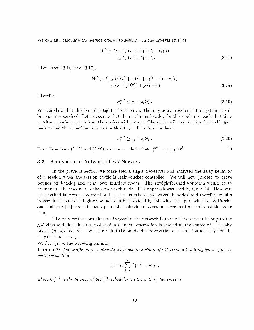
Corollary 1: Let � be the start of the jth network busy period of session i in a network of LRservers. If �i is the minimum bandwidth allocated to session i in the network, the service o�ered topackets of the jth network busy period after the kth node in the network is given byWSki;j (�; t) � max0@0; �i(t� � � kXj=1�(Sj)i )1A ;where �(Sj)i is the latency of the jth server in the network for session i.Using the above corollary we can bound the end-to-end delays of session i if the input tra�cis leaky-bucket shaped and the average arrival rate is less than �i.Theorem 2: The maximum delay Di of a session i in a network of LR servers, consisting of Kservers in series, is bounded as Di � �i�i + KXj=1�(Sj)i ; (3.32)where �(Sj)i is the latency of the jth server in the network for session i.Proof: From Corollary 1, we can treat the whole network as equivalent to a single LR-server withlatency equal to the sum of their latencies. By using Theorem 1, we can directly conclude that themaximum delay is Di � �i�i + kXj=1�(Sj)i : 2This maximum delay is independent of the topology of the network. The bound is alsomuch tighter than what could be obtained by analyzing each server in isolation. Note that theend-to-end delay bound is a function of only two parameters: the burstiness of the session tra�c atthe source and the latencies of the individual servers on the path of the session. Since we assumedonly that each of the servers in the network belongs to the LR class, these results are more generalthan the delay bounds due to Parekh and Gallager [16]. In the next section, we will show that allwell-known work-conserving schedulers are in fact LR servers. Thus, our delay bound applies toalmost any network of schedulers.The delay bound in Eq. (3.32) shows that there are two ways to minimize delays and bu�errequirements in a network of LR servers: i) allocate more bandwidth to a session, thus reducingthe term �i=�i, or ii) use LR servers with low latencies. Since the latency is accumulated throughmultiple nodes, the second approach is preferred in a large network. The �rst approach reducesthe utilization of the network, thus allowing only a smaller number of simultaneous sessions tobe supported than would be possible with minimum-latency servers. Minimizing the latency alsominimizes the bu�er requirements of the session at the individual servers in the network.Proposition 1: The end-to-end delay and increase in burstiness of a session in a network of LRservers is proportional to the latency �Si of the servers. We can minimize both of these parametersby designing servers with minimum latency. 19

Note that the latency of a server depends, in general, on its internal parameters and thebandwidth allocation of the session under consideration. In addition, the latency may also varywith the number of active sessions and their allocations. Such a dependence of the latency of onesession on other sessions indicates the poor isolation properties of the scheduler. Likewise, in someschedulers the latency may depend heavily on its internal parameters, and less on the bandwidthallocation of the session under observation. Such schedulers do not allow us to control the latency ofa session by controlling its bandwidth allocation. On the other hand, the latency of a PGPS serverdepends heavily on the allocated bandwidth of the session under consideration. This exibility isgreatly desirable.3.3 Delay Bound for Sessions with Known Peak RateSince the de�nition of an LR server is not based on any assumptions on the input tra�c,it is easy to derive delay bounds for tra�c distributions other than the (�; �) model. For example,when the peak rate of the source is known, a modi�ed upper bound on the delay of an LR servercan be obtained. Let us denote with gi the service rate allocated to connection i, and let �i andPi respectively denote the average and peak rate at the source of connection i. The arrivals at theinput of the server during the interval (�; t] now satisfy the inequalityAi(�; t) � min (�i + �i(t� �); Pi(t� �)) : (3.33)We can prove the following lemma:Lemma 5: The maximum delay Di of a session i in an LR server, where the peak rate of thesource is known, is bounded as DSi � �Pi � gigi �� �iPi � �i�+ �Si : (3.34)Proof: Let us assume that the maximum delay DSi was obtained for a packet that arrived at timet� during the jth busy period. This means that the packet was serviced at time t� +DSi . Hence,the amount of service o�ered to the session until time t�+DSi is equal to the amount of tra�c thatarrived from the session until time t. Since sj is the beginning of the jth busy period,WSi;j(sj ; t� +DSi ) = Ai(sj ; t�): (3.35)From Eq. (3.33), this becomesWSi;j(sj ; t� +DSi ) � min (�i + �i(t� � sj); Pi(t� � sj)) : (3.36)Since the server may provide no service for time �Si , DSi � �Si . From the de�nition of LR-server,WSi;j(sj ; t� +DSi ) � gi(t� +DSi � sj ��Si ): (3.37)From (3.36) and (3.37), we havegi(t� +DSi � sj ��Si ) � min (�i + �i(t� � sj); Pi(t� � sj)) : (3.38)20

Case 1: When Pi(t� � sj) � �i + �i(t� � sj), we haveDSi � �Pi � gigi � (t� � sj) + �Si ; (3.39)and Pi(t� � sj) � �i + �i(t� � sj);or, t� � sj � �iPi � �i :Substituting for (t� � sj) in Eq. (3.39), we getDSi � �Pi � gigi �� �iPi � �i�+ �Si : (3.40)Case 2: When Pi(t� � sj) > �i + �i(t� � sj), we get(t� � sj) > �iPi � �i : (3.41)From Eq. (3.38), (gi � �i)(t� � sj) � �i � giDSi + gi�Si ; (3.42)and by substituting for t� � sj from Eq. (3.41),DSi � �Pi � gigi �� �iPi � �i�+ �Si : (3.43)2A network of LR servers can be modeled as a single LR server with latency equal to thesum of the latencies. Thus, the following main result can be derived:Corollary 2: The maximum delay Di of a session i in a network of LR servers, consisting of Kservers in series, where the peak rate of the source is known, is bounded asDi � �Pi � gigi �� �iPi � �i�+ KXj=1�Sji : (3.44)where �Sji is the latency of the jth node.4 Schedulers in the Class LRIn this section we will show that several well-known work-conserving schedulers belong tothe class LR and determine their latencies. Recall that our de�nition of LR servers in the previoussection is based on session-busy periods. In practice, however, it is easier to analyze schedulingalgorithms based on session backlogged periods. The following lemma enables the latency of anLR server to be estimated based on its behavior in the session backlogged periods. We will usethis as a tool in our analysis of several schedulers in this section.21

Lemma 6: Let (sj ; tj ] indicate an interval of time in which session i is continuously backlogged inserver S. If the service o�ered to the packets that arrived in the interval (sj ; tj ] can be bounded atevery instant t, sj < t � tj as Wi(sj ; t) � max(0; �i(t� sj � �i));then S is an LR server with a latency less than or equal to �i.This lemma will allow us to estimate the latency of an LR-server. However, it does notnecessarily provide us a tight bound for the parameter �i. An easy way to determine if the boundis tight is to present at least one example in which the o�ered service is actually equal to the bound.This is the approach we will take in this section to determine the latencies of several LR servers.Proof: We will prove the lemma by induction on the number of busy periods. Let us use (�k; �k]to denote the kth busy period of session i in the server.Base step: At time �1, the beginning of the �rst session-i busy period, the system becomesbacklogged for the �rst time. Let us assume that the �rst busy period consists of a number ofbacklogged periods (sj ; tj ]. By the de�nition of session busy period, the following inequality musthold at the beginning of the jth backlogged period:A(�1; sj) � �i(sj � �1):However, the system is empty at time sj . Therefore,A(�1; sj) = Wi;1(�1; sj): (4.1)Consider any time t in the interval (sj ; tj]. We can writeWi(�1; t) = Wi;1(�1; t)= Wi;1(�1; sj) +Wi;1(sj ; t)� �i(sj � �1) + max(0; �i(t� sj � �i))� max(0; �i(t� �1 � �i)) (4.2)Now consider any time t within the busy period, but between two backlogged periods; thatis, tj � t � sj+1. Since session i receives no service during the interval (t; sj+1], we can writeWi(�1; t) = Wi;1(�1; t) = Wi;1(�1; sj+1): (4.3)But, Wi;1(�1; sj+1) = Ai(�1; sj+1)� �i(sj+1 � �1)� �i(t� �1): (4.4)Therefore, from (4.3) and (4.4), Wi(�1; t) � �i(t� �1): (4.5)22

Combining (4.2) and (4.5), we can conclude that, at any instant t during the �rst busy period(�1; �1], Wi(�1; t) � max(0; �i(t� �1 � �i)): (4.6)Inductive step: Assume that the lemma is true for all busy periods 1; 2; : : : ; n. We will now provethat the lemma is true for the (n+ 1)th busy period as well.If the system is not backlogged when the (n + 1)th busy period starts, we can repeat thesame proof as in the base step. However, it is possible that, when the (n+ 1)th busy period starts,the system is still backlogged with packets from the nth or earlier busy periods. Let us assumethat the backlogged period in progress when the (n+1)th busy period starts is the mth backloggedperiod. This backlogged period started at time sm; in the general case, we can assume that packetsfrom L earlier busy periods were serviced during the backlogged period (sm; tm]. Let � denote theinstant at which the last packet from the nth busy period was serviced. Then,Wi(sm; �) = nXj=n�LAi(�j ; �j)�Wi;n�L(�n�L; sm)� �i(�n � �n�L)� �i(sm � �n�L)� �i(�n � sm) (4.7)We need to show that Wi;n+1(�n+1; t) � max(0; �i(t � �n+1 ��i)). We can proceed as follows:Wi;n+1(�n+1; t) = Wi(�; t)= Wi(sm; t)�Wi(sm; �)� max(0; �i(t� sm � �i))� �i(�n � sm)� max(0; �i(t� �n ��i))� max(0; �i(t� �n+1 � �i):The last inequality follows from the fact that �n < �n+1 and that the service o�ered to a session cannever be negative. If, after time t, the packets of the (n+1)th busy period form multiple backloggedperiods, the proof for the base step can be repeated to complete the proof of the lemma. 2A main contribution of the theory of LR-servers is the notion of the busy period. Thebound on the service o�ered by an LR-server is based on the busy period. This is a more generalapproach than bounding the service o�ered by the server based on the concept of the backloggedperiod. An approach based on the latter was proposed in [23] for providing QoS guarantees. Thismodel bounds the service o�ered to a connection during one or more backlogged periods, thusproviding a means to design a class of scheduling algorithms that can provide speci�c end-to-enddelay guarantees. Using the concept of busy period instead of backlogged period in this model willlikely result in tighter end-to-end delay bounds and a larger class of schedulers that can providethese delay bounds.In Lemma 6 we proved that, if we use the backlogged period to bound the service o�eredby a server S, then S is an LR server and its latency can not be larger than that found for thebacklogged period. However, we must emphasize the fact that the opposite is not true. Consider23

Θ

ρ ρ

Θ b

ρ

A(0,t)

0 t t1 2

W(0,t)

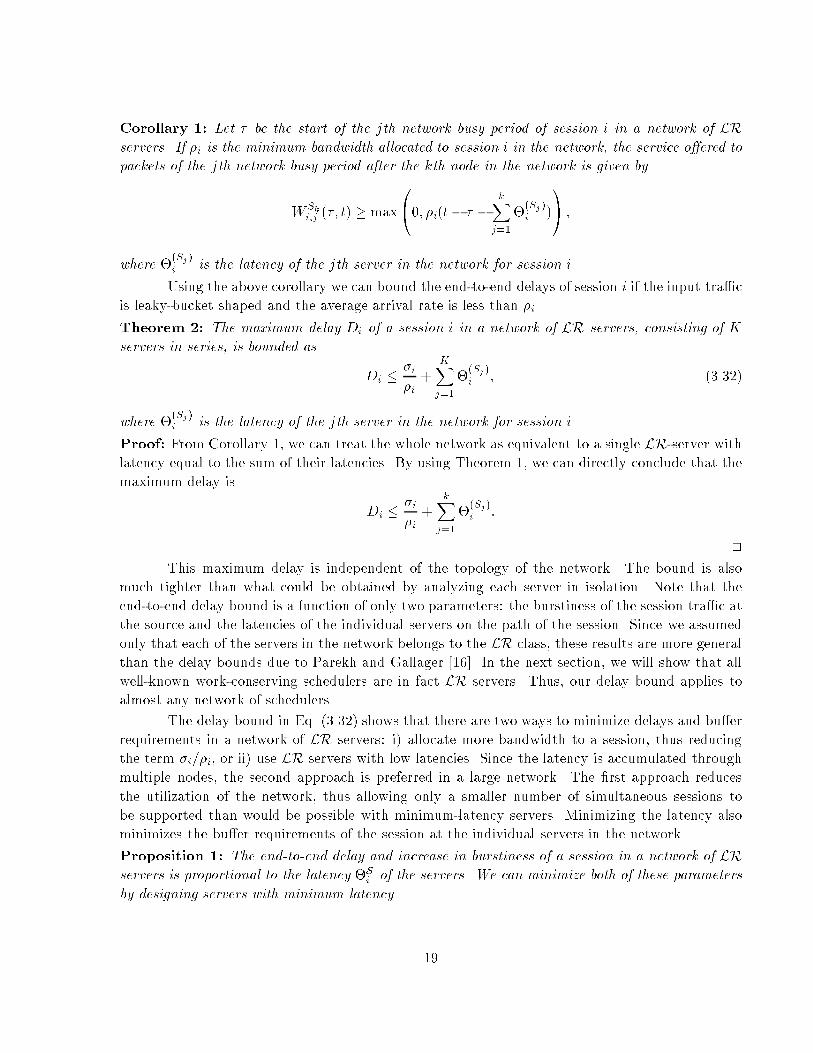
t 3Figure 4.1: Di�erence in bounding service based on the backlogged and busy periods.Server LatencyGPS 0PGPS Li�i + LmaxrSCFQ Li�i + Lmaxr (V � 1)VirtualClock Li�i + LmaxrDe�cit Round Robin 3F�2�irWeighted Round Robin F��i+LcrTable 4.1: Some LR servers and their latencies. Li is the maximum packet size of sessioni and Lmax the maximum packet size among all the sessions. In weighted round-robinand de�cit round-robin, F is the frame size and �i is the amount of tra�c in the frameallocated to session i. Lc is the size of the �xed packet (cell) in weighted round-robin.the example of Figure 4.1. Let us assume an LR-server with rate � and latency �. Referring toFigure 4.1, time-intervals (0; t1] and (t2; t3] form two busy periods. However, the server remainsbacklogged during the whole interval (t1; t3]. If the backlogged period was used to bound the serviceo�ered by the server, a latency �b > � would result. By extending the above example over multiplebusy periods, it is easy to verify that �b can not be bounded. This shows that if backlogged periodwas used instead of busy period in the de�nition of the LR server model, the end-to-end delays ofthe server would not be bounded.By using the above lemma as our tool, in Appendix 7 we analyze several work conservingservers and prove that they belong in the class LR. A summary of our results is presented inTable 4.1.It is easy to see that PGPS and VirtualClock have the lowest latency among all the servers.In addition, their latency does not depend on the number of connections sharing the same outgoinglink. As we will show in Section 6, however, that VirtualClock is not a fair algorithm.24

In self-clocked fair queueing, the latency is a linear function of the maximum number ofconnections sharing the outgoing link. In De�cit Round Robin, the latency depends on the framesize F . By the de�nition of the algorithm, the frame size, in turn, is determined by the granularityof the bandwidth allocation and the maximum packet size of its session. That is,VXi=1Li � F;where Li is the maximum packet-size of session i. Thus, the latency in De�cit Round Robin is alsoa function of the number of connections that share the outgoing link. Weighted Round Robin canbe thought of as a special case of De�cit Round Robin and its latency is again a function of themaximum number of connections sharing the outgoing link.5 An Improved Delay BoundThe latencies of LR servers computed in the last section are based on the assumption thata packet is considered serviced only when its last bit has left the server. Thus, the latency �Siwas computed such that the service performed during a session busy period at time t, Wi;j(�; t), isalways greater than or equal to �i(t � � � �Si ). Since the maximum di�erence between Wi;j(�; t)and �i(t� �) occurs just before a session-i packet departs the system, the latency �Si is calculatedat such points. This is necessary to be able to bound the arrivals to the next server in a chain ofservers; since our servers are not cut-through devices, a packet can be serviced only after its lastbit has arrived. Our assumption that the packet leaves as an impulse from the server allows us tomodel the arrival of the packet in the next server as an impulse as well.When we compute the end-to-end delay of a session, however, we are only interested in�nding the time at which the last bit of a packet leaves the last server. Thus, for the last serverin a chain, we can determine the latency �Si based only on the instants of time just after a packetwas serviced from the session. This results in a lower value of latency and, consequently, a tighterbound on the end-to-delay in a network of servers than that given by eq. (3.32).To apply this idea, the analysis of the network is separated into two steps. If the sessionpasses through k hops, we bound the service o�ered to the session in the �rst k�1 servers consideringarbitrary instants during session-busy periods. On the last node, however, we calculate the latencybased only on the points just after a packet completes service.This idea is best illustrated by an example in the case of the PGPS server. Assume that abusy period starts at time � , and that a packet leaves the PGPS server at time tk. Then, on thecorresponding GPS server, this packet left at time tk � Lmax=r or later. Therefore, if we consideronly such points tk , we can writeWPi;j(�; tk) � WFi;j(�; tk � Lmaxr )� �i(tk � � � Lmaxr ):This results in a latency of Lmax=r as compared to (Li=�i + Lmax=r) computed in eq. (A.1).25

Lmaxr

Lmax + Lir i

Ai(t)Wi(t)

Latency for delayLatency for traffic

θ i =Figure 5.1: Illustration of the two envelopes used to bound the service received by session iin a session-busy period. Each step in the arrival function indicates a new packet. Thelower envelope is a valid lower-bound for the service at any point in the busy period, whilethe upper one is valid only at the points when a packet leaves the system.Figure 5.1 shows the two envelopes based on bounding the service received by the session inthe two di�erent ways. The lower envelope applies to arbitrary points in the session-busy period,while the upper envelope is valid only at points when a packet leaves the system. For computingend-to-end delay bounds in a network of servers, we can use the upper envelope in the last server. Inall the work-conserving schedulers we have studied, the two envelopes are apart by Li=�i, where Li isthe maximum packet-size for session i. Therefore, for these LR servers, we can obtain an improvedbound for the end-to-end delay in a network by subtracting Li=�i from eq. (3.32). Therefore,Di � �i�i + kXj=1�(Sj)i � Li�i : (5.1)If we substitute the latency obtained for PGPS from eq. (A.1) in this expression, that is,�(Sj)i = Li=�i + Lmax=r, we get Di � �i�i + (k � 1)Li�i + kLmaxr ; (5.2)which agrees with the bound obtained by Parekh and Gallager [16] for a network of PGPS servers.Since the latencies of PGPS and VirtualClock are identical, the bound of (5.2) applies to Virtual-Clock as well; this is also in agreement with the results of Lam and Xie [24].While we have veri�ed that this improvement of Li=�i in the delay bound is valid for allthe LR servers analyzed in this paper, whether this is true for all LR servers remains an openquestion. We have not yet found a formal proof on its validity for arbitrary LR servers.26

6 Fairness of LR ServersIn Section 3, we showed that the worst-case delay behavior of individual sessions in a networkof LR servers can be analyzed knowing only their latencies. However, the latency of an LR server,by itself, provides no indication of its fairness. For example, VirtualClock and PGPS are twodi�erent LR servers with the same latency, but with substantially di�erent fairness characteristics.In this section we analyze the fairness characteristics of several well-known LR servers and comparethem. The fairness parameter that we use is based on the de�nition presented by Golestani [5]for analysis of self-clocked fair queueing. Let us assume that WSi (�; t) is the service o�ered toconnection i in the interval (�; t] by server S. If �i is the bandwidth allocated to connection i, wewill call the fraction WSi (�; t)=�i the normalized service o�ered to connection i in the interval (�; t].A scheduler is perfectly fair if the di�erence in normalized service o�ered to any two connectionsthat are continuously backlogged in the system in the interval (�; t] is zero. That is,�����WSi (�; t)�i � WSi (�; t)�j ����� = 0:GPS multiplexing is proven to have this property. However, this condition cannot be met byany packet-by-packet algorithm since packets must be serviced exclusively. Therefore, in a packetby packet server, we can only require that the di�erence in normalized service received by theconnections be bounded by a constant.Golestani [5] suggested use of the di�erence in normalized service o�ered to any twoconnections as the measure of fairness for the algorithm [5]. More precisely, an algorithm isconsidered close to fair if, for any two connections i; j that are continuously backlogged in aninterval of time (t1; t2], �����WSi (t1; t2)�i � WSj (t1; t2)�j ����� � FS ;where FS is a constant. Let us call FS as the fairness of server S. A di�culty arises, however, in theuse of the above de�nition in comparing the fairness of di�erent schedulers. For the same patternof session arrivals, the backlogged periods of the session can vary across schedulers; a comparisonof fairness of di�erent scheduling algorithms can therefore yield misleading results if the arrivalpattern is not chosen so as to produce the same backlogged periods in all the schedulers. Hence, wemodify Golestani's de�nition slightly. We consider a time � at which the connections i and j beingcompared have an in�nite supply of packets. This forces them to be continuously backlogged in theservers, regardless of the scheduling algorithm used. We use as a measure of fairness the di�erencein normalized service o�ered to the two connections for any time interval (t1; t2] after time � .A typical example of unfairness occurs in the VirtualClock algorithm, as illustrated inFigure 6.1. Assume that two connection share an outgoing link and are allocated equal shares ofthe link bandwidth. Assume each packet is of unit size and the rate of the server is also unity.Consider an interval of time 0{1000 during which only connection 1 is active, and sends 1000 packets.Connection 2 becomes active at time 1000, and both connections send packets after 1000. Assumethat the scheduler is based on the VirtualClock algorithm. Since the server is work-conserving,27

............

......

......

0

............

......

1000 1500

............

VirtualClock

1

2

PGPSFigure 6.1: Unfair behavior of the VirtualClock scheduling algorithm. The two connectionsare allocated equal portions of the outgoing link bandwidth.it will service all 1000 packets from connection 1 by t = 1000. However, at time t = 1000, thenext arriving packet of connection 1 will receive a timestamp of 2000, re ecting the average servicereceived by the connection until 1000. Thus, connection 1 will be starved until time 1500, whenthe timestamps of the packets of the two connections become equal. If the maximum burstinessof the sources is not bounded, we can see that the interval over which a backlogged connection isdenied service can grow to in�nity. A PGPS server, in contrast, provides equal service to the twoconnection after t = 1000, regardless of the excess bandwidth received by connection 1 earlier.We now evaluate the fairness of a number of well-known servers. We use Li to denotethe maximum packet-size for session i and Lmax the maximum packet-size over all sessions. ForVirtualClock, we have already seen that there is no �nite value of FS satisfying our de�nition offairness.6.1 Fairness of a PGPS SchedulerBased on the above measure of fairness, the fairness of a PGPS server is given by thefollowing lemma. A detailed proof of the lemma can be found in [25].Lemma 7: For a PGPS scheduler,FS = max(max(Cj + Lmax�i + Lj�j ; Ci + Lmax�j + Li�i )where Ci is the maximum normalized service that a session may receive in a PGPS server in excessof that in the GPS server, given byCi = min�(V � 1)Lmax�i ; max1�n�V (Ln�n )� :It can be shown that the above bound is tight. 28

6.2 Fairness of Self-Clocked Fair QueueingGolestani [5] proved the following bound for SCFQ:FS = Li�i + Lj�j :We now prove that this bound is tight by presenting an example where the bound is actuallyreached.Let us assume that at time t1, the kth packet from connection i has just been serviced bythe SCFQ server. The next packet will have a virtual �nishing time equal toF k+1i = F ki + Li�i :Packets from connection j may be serviced after the kth packet of connection i, as long as theirvirtual �nishing times are less than or equal to F k+1i . Let us assume that connection j has a packetx of size Lj with the same �nishing time F ki . Assume also that j has a set of packets queued behindx with total size equal to Li�i �j :The last of these packets will get a virtual �nishing time ofFmj = F ki + Li�i :Therefore, a total amount of tra�c equal to Lj + Li�i �j may be serviced from connection j beforethe (k + 1)th packet from connection i is serviced. Let t2 be time at which the packets of j �nishservice. Then, Wj(t1; t2)�j � Wi(t1; t2)�i = 1�j (Lj + Li�i �j)= Li�i + Lj�j :6.3 Fairness of a Round-Robin SchedulerDe�cit Round Robin was proposed by Sreedhar and Varghese [8] as an O(1) algorithm forproviding bandwidth guarantees in an output-bu�ered switch. De�cit Round Robin is a generaliza-tion of the Weighted-Round-Robin algorithm that was proposed in the context of ATM networks [7].The latter assumes that packets from all connections have the same size and connections are ser-viced in a round-robin order. The time is split into frames of maximum size F and a connectionis not allowed to send more than �i packets during a frame period. Therefore, the bandwidthallocated to a connection is �i � �iF r;29

De�cit Round Robin estimates the service o�ered to a connection during a round in terms of bytesand not in terms of packets, allowing it to be used with variable-size packets. Connections areserviced in a round-robin fashion. Once a connection is selected, up to �i bytes may be sent forthat connection. If the transmission of a whole packet forces the connection to send more than �ipackets, the last packet is not sent and a de�cit counter Dki is updated, indicating the service thatwas missed from the connection during the kth round. This de�cit is then added to �i in the nextround while servicing tra�c from connection i.Another variation of the round-robin service disciplines is the Surplus Round Robin (SRR)[26, 27]. The di�erence of this policy from De�cit Round Robin is that, if a packet forces theconnection to send more than �i bytes in a frame, the packet is sent and a surplus counter Ski isupdated to re ect the amount of excess service that was o�ered to the connection during the kthround. This service will be lost during the next round.It has been shown that, in the De�cit Round Robin algorithm, the di�erence in serviceo�ered to any two connections that have the same bandwidth reservation is bounded by 3�i, where�i is the number of bytes allocated to these connections in each frame [8]. Here we extend theresult to the case of two connections with arbitrary bandwidth allocations.Lemma 8: For a De�cit-Round-Robin scheduler,FS = 3Fr :Proof: Let us assume a time interval (t0; tn], where t0 is the beginning of a round and tn is the endof the nth round after t0. For each k = 1; 2 : : : ; n when the connection is continuously backlogged,Wi(tk�1; tk) = �i +Dk�1i �Dki ; (6.1)where Dki is the value of the de�cit counter of connection i at the end of the kth round. Summingover k, Wi(t0; tk) = k�i +D0i �Dki : (6.2)Since Dki � �i, for every k, we can writeWi(t0; tk) � k�i + �i: (6.3)Similarly, if connection j is continuously backlogged over the same interval, we can writeWj(t0; tk) = k�j +D0j �Dkj :� k�j � �j : (6.4)From equations (6.3) and (6.4) we can easily conclude that�����Wi(t0; tk)�i � Wj(t0; tk)�j ����� � �i�i + �j�j� 2Fr :30

This bound applies to time intervals that span complete frames. For an arbitrary interval, thedi�erence in service o�ered to the two connections may increase by another �i or �j bytes. Bynormalizing this additional di�erence, we can obtain the general bound for fairness asFS = 3Fr : (6.5)2In the case of Weighted Round Robin, where the de�cit is always zero across the rounds,an extension of the above proof will lead us to the following corollary:Corollary 3: For a Weighted-Round-Robin scheduler,FS = Fr :In concluding this section, we note that all the algorithms studied, except VirtualClock,can be considered as fair based on our de�nition of fairness. However, it is interesting to note thatself-clocked fair queueing (SCFQ) has the best fairness among all the packet-by-packet schedulers,even better than that of PGPS in some cases. On the other hand, the latency of an SCFQ server canbe much higher than that of a PGPS server; this is because SCFQ may delay service to connectionswhen they become backlogged after an idle period, while PGPS penalizes the connections that havealready received their allocated bandwidth to serve newly backlogged connections.7 ConclusionsIn Table 2, we have summarized the characteristics of several scheduling algorithms belong-ing to the LR class based on the three parameters discussed in Section 2. Based on this summary,it is easy to see that the PGPS scheduler has the best performance both in terms of latency andfairness properties. However, it also has the highest implementation complexity. VirtualClock haslatency identical to that of PGPS, but is not a fair algorithm.All the other algorithms studied have bounded unfairness, but also have much higherlatencies than PGPS. From our analysis of networks of LR servers, it becomes clear how thisincreased latency leads to high end-to-end delay bounds, large bu�er requirements in the switchnodes, and increased tra�c burstiness inside the network. Even with constant-bit-rate tra�c atthe source, sessions may accumulate considerable burstiness after many hops through the networkif the the servers have high latencies. Thus, the use of servers with minimum latency is extremelyimportant in a broadband packet network. In both the SCFQ server and the round-robin schedulers,the latency and fairness are greatly a�ected by the number of connections sharing a commonoutgoing link. This property makes it di�cult to control end-to-end session delays in networkswhere a large number of ows may share the links.Our comparison of schedulers along the three dimensions leaves open the question whethera scheduling algorithm can be designed that has the same low latency as that of PGPS, boundedunfairness, and an e�cient implementation. In [25], we extend this work by presenting such ascheduling discipline that we call Frame-based Fair Queueing (FFQ). FFQ is a sorted-priorityalgorithm in which the calculation of timestamps can be performed in O(1) time. The latency of31

Server Latency Fairness ComplexityGPS 0 0 -PGPS Li�i + Lmaxr max(max(Cj+Lmax�i +Lj�j ; Ci+Lmax�j +Li�i ), whereCi = min((V � 1)Lmax�i ; max1�n�V (Ln�n )). O(V )SCFQ Li�i + Lmaxr (V � 1) Li�i + Lj�j O(logV )VirtualClock Li�i + Lmaxr 1 O(logV )De�cit Round Robin (3F�2�i)r 3Fr O(1)Weighted Round Robin (F��i+Lc)r Fr O(1)Frame-Based FairQueueing (FFQ) [25] Li�i + Lmaxr max(2F��ir + Li�i ; 2F��ir + Lj�j ;Lmax�j + Li�i ; Lmax�i + Lj�j ) O(logV )Table 7.1: Latency, fairness and implementation complexity of several work-conservingservers. Li is the maximum packet size of session i and Lmax the maximum packet sizeamong all the sessions. Ci is the maximum normalized service that a session may receivein a PGPS server in excess of that in the GPS server. In weighted round-robin and de�citround-robin, F is the frame size and �i is the amount of tra�c in the frame allocated tosession i. Lc is the size of the �xed packet (cell) in weighted round-robin.frame-based fair queueing is identical to that of a PGPS server, yet the algorithm can be shown tobe fair based on the criterion we used in this paper to evaluate fairness.It should be noted that our approach of modeling a network of LR servers as a singleLR server did not make any assumptions about the input tra�c. Although the bounds derivedin this paper for the end-to-end delays and bu�er requirements hold only when the input tra�cis leaky-bucket shaped, the same model can be used for analysis with other input-tra�c models.For example the Exponentially-Bounded-Burstiness (EBB) model was used in [28, 29] for analyzingthe behavior of a GPS multiplexer. Future work will include the use of other tra�c models forproviding end-to-end delay guarantees in a network of LR servers.The fairness analysis presented in Section 6 did not cover the intervals of time wherea connection may be idle. A more complete analysis should include such intervals. In a fairalgorithm, the service lost by two connections while they were idle should also be proportional totheir reservations. In addition, if one connection is idle and the other backlogged, the idle connectionmust be losing normalized service proportional to the service that the backlogged connection isreceiving. Future work will include the de�nition of a universal method for estimating the fairnessof a scheduling algorithm. This measure must depend only on the characteristics of the server, and32

not on the tra�c parameters of individual sessions. However, it must be a su�cient condition toprove that the server is providing service to a connection comparable to that provided by by a GPSmultiplexer.References[1] D. D. Clark, S. Shenker, and L. Zhang, \Supporting real-time applications in an integratedservices packet network: Architecture and mechanism," in Proceedings of ACMSIGCOMM '92,pp. 14{26, August 1992.[2] L. Zhang, \VirtualClock: a new tra�c control algorithm for packet switching networks," ACMTransactions on Computer Systems, vol. 9, pp. 101{124, May 1991.[3] A. Demers, S. Keshav, and S. Shenker, \Analysis and simulation of a fair queueing algorithm,"Internetworking: Research and Experience, vol. 1, no. 1, pp. 3{26, 1990.[4] A. K. Parekh and R. G. Gallager, \A generalized processor sharing approach to ow control -the single node case," in Proceedings of INFOCOM '92, vol. 2, pp. 915{924, May 1992.[5] S. Golestani, \A self-clocked fair queueing scheme for broadband applications," in Proceedingsof INFOCOM '94, pp. 636{646, IEEE, April 1994.[6] D. Ferrari and D. Verma, \A scheme for real-time channel establishment in wide-area networks,"IEEE Journal on Selected Areas in Communications, vol. 8, pp. 368{379, April 1990.[7] M. Katevenis, S. Sidiropoulos, and C. Courcoubetis, \Weighted round-robin cell multiplexingin a general-purpose ATM switch chip," IEEE Journal on Selected Areas in Communications,vol. 9, pp. 1265{79, October 1991.[8] M. Shreedhar and G. Varghese, \E�cient Fair Queueing using De�cit Round Robin," in Proc.SIGCOMM'95, September 1995.[9] C.Kalmanek, H.Kanakia, andS.Keshav, \Rate controlled servers for veryhigh-speednetworks,"in IEEE Global Telecommunications Conferece, pp. 300.3.1{300.3.9, December 1990.[10] S. Golestani, \A framing strategy for congestion management," IEEE Journal on Selected Areasin Communications, vol. 9, pp. 1064{1077, September 1991.[11] D. Verma, D. Ferrari, and H. Zhang, \Guaranteeing delay jitter bounds in packet switchingnetworks," in Tricomm 91, April 1991.[12] H. Zhang and S. Keshav, \Comparison of rate based service disciplines," in Proceedings of ACMSIGCOMM '91, pp. 113{122, 1991.[13] R. Cruz, \A calculus for network delay. I. Network elements in isolation.," IEEE Transactionson Information Theory, vol. 37, pp. 114{131, January 1991.[14] R. Cruz, \A calculus for network delay. II. Network elements in isolation.," IEEE Transactionson Information Theory, vol. 37, pp. 132{141, January 1991.[15] H. Zhang, Service Disciplines for Packet-Switching Integrated-Services Networks. PhD thesis,U.C. Berkeley, 1992.[16] A. K. Parekh and R. G. Gallager, \A generalized processor sharing approach to ow control inintegrated services networks: the multiple node case," in Proceedings of INFOCOM '93, vol. 2,pp. 521{530, March 1993. 33

[17] P. Goyal, S. Lam, and H. Vin, \Determining end-to-end delay bounds in heterogeneous net-works," in Proceedings of the 5th International Workshop on Network and Operating SystemSupport for Digital Audio and Video, pp. 287{298, April 1995.[18] S. Golestani, \Network delay analysis of a class of fair queueuing algorithms," IEEE Journalon Selected Areas in Communications, vol. 13, pp. 1057{70, August 1995.[19] J. Turner, \New directions in communications (or which way to the information age?)," IEEECommunications Magazine, vol. 24, pp. 8{15, October 1986.[20] T. Cormen, C. Leiserson, and R. Rivest, Introduction to Algorithms. New York: McGraw Hill,1989.[21] R. Brown, \Calendar queues: a fast 0(1) priority queue implementation for the simulation eventset problem," Communications of the ACM, vol. 31, pp. 1220{1227, October 1988.[22] H. Chao and N. Uzun, \A VLSI sequencer chip for ATM tra�c shaper and queue manager,"IEEE Journal of Solid-State Circuits, vol. 27, pp. 1634{1643, November 1992.[23] R. Cruz, \Quality of service guarantees in virtual circuit switched networks," IEEE Journal onSelected Areas In Communications, vol. 13, pp. 1048{1056, August 1995.[24] S. Lam and G. Xie, \Burst scheduling: Architecture and algorithm for switching packet video,"in INFOCOM'95, April 1995.[25] D. Stiliadis and A. Varma, \Frame-based fair queueing: A new tra�c scheduling al-gorithm for packet-switched networks," Tech. Rep. UCSC-CRL-95-39, U.C. Santa Cruz,http://www.cse.ucsc.edu/research/hsnlab/publications/, July 1995.[26] H. Adiseshu, G. Parulkar, and G. Varghese, \Reliable FIFO load balancing over multiple �fochannels," tech. rep., Washington University, St. Louis, May 1995.[27] S. Floyd, \Notes on guaranteed service in resource management." Unpublished notes, 1993.[28] O. Yaron and M. Sidi, \Performance and stability of communication networks via robustexponential bounds," IEEE/ACMTransactions on Networking, vol. 1, pp. 372{385, June 1993.[29] Z. Zhang, D. Towsley, and J. Kurose, \Statistical analysis of generalized processor sharingscheduling discipline," in Proceedings of ACM SIGCOMM '94, pp. 68{77, September 1994.34

Appendix A: Schedulers in the Class LR and Their LatenciesThis appendix contains the proofs for showing that many well-known scheduling algorithmsbelong to the class of LR servers and derives their latencies. In the following proofs, Li denotesthe maximum packet-size for session i and Lmax the maximum packet-size among all sessions.A.1 Weighted-Fair-QueueingWe �rst start by showing that a GPS scheduler is an LR server.Lemma 9: A GPS scheduler belongs to the class LR and its latency is zero.Proof: From the de�nition of the GPS multiplexer, during any interval of time that connection iis continuously backlogged, WGPSi (�; t) � �i(t� �):From Lemma 6 it easy to conclude that a GPS scheduler is an LR-server with zero latency. 2Weighted-Fair-Queueing or Packet-by-packet GPS (PGPS) scheduling algorithm is thepacket-by-packet equivalent of GPS multiplexing. In [4] it was proven that, if tF ; tP are the timesthat a packet �nishes under WFQ and GPS, respectively, thentP � tF + Lmaxr ;where r is the transmission rate of the server. For the analysis of a network of LR servers itis required that the service be bounded for any time after the beginning of a busy period. Inaddition, we can only consider that a packet left a packet-by-packet server if all of its bits have leftthe server. These requirements are necessary in order to provide accurate bounds for the tra�cburstiness inside the network. Therefore, just before time tP the whole packet has not yet departedthe packet-by-packet server. Let Li be the size of the packet. The service o�ered to connection i inthe packet-by-packet server will be equal to the service o�ered to the same connection by the GPSmultiplexer until time tP minus this last packet. Notice also that in a GPS multiplexer, since thelatency is zero, the beginning of a busy period �nds the system always empty. Therefore,WPi;j(�; t) � WFi;j(�; t� Lmaxr )� Li� max(0; �i(t� � � Lmaxr )� Li)� max(0; �i(t� � � Lmaxr � Li�i )):Hence, we can state the following corollary:Corollary 4: Weighted-Fair-Queueing is an LR server with latencyLmaxr + Li�i :This latency can be shown to be tight. 35

A.2 VirtualClockThe VirtualClock service discipline is based on the calculation of a timestamp for eachpacket that arrives in the system. The timestamp is calculated based on the timestamp of theprevious packet of the same connection and the real time that passed after the beginning of thesystem busy period. In [25], we prove the following theorem that classi�es VirtualClock as an LRserver.Theorem 3: The VirtualClock service discipline is an LR server and its latency isLmaxr + Li�i :A.3 Self-Clocked Fair QueueingIn this section we will analyze the self-clocked fair queueing (SCFQ) algorithm and provethat it is also an LR-server. SCFQ was proposed as a simpli�cation of the PGPS server and is asorted-priority algorithm. When a connection becomes backlogged, the virtual time is estimated bythe virtual �nishing time of the packet that is being serviced. Let TScur indicate this time. Then,the virtual �nishing time of the jth packet of connection i is estimated asF ji = max(F j�1i ; TScur) + Lji�i ;where Lji is the length of the jth packet of connection i. Packets are always serviced in increasingorder of their virtual �nishing times. When the system becomes empty, all variables are reset tozero. Let us assume that a connection becomes backlogged at time � and let this be the kthpacket of the connection. We �rst prove the following lemma:Lemma 10: If the kth packet of session i starts a backlogged period in SCFQ server, its virtual�nishing time will be estimated by the system virtual time:F ki = TScur + Lji�k :Proof: We will prove the lemma by contradiction. Let us assume thatF k�1i > TScur :Then, the packet F k�1i has not been serviced yet and thus the kth packet does not �nd the systemempty. 2We can now prove the following theorem:Theorem 4: At ant time t during a session i backlogged period in an SCFQ server,Wi(�; t) � �i(t� � � (V � 1)Lmaxr � Li�i ):36

Proof: Let � be the start of a backlogged period for session i in the SCFQ server. Assume thatthe backlogged period was started by the arrival of the kth packet of session i. By Lemma 10, thevirtual �nishing time of this packet will beF ki = TScur + Lji�i : (A.1)Consider the nth of the same backlogged period of session i, that is, the (k + n � 1)th packet ofsession i. Let us mark this packet. The virtual �nishing time of this packet will beF k+n�1i = TScur + nLi�i : (A.2)Let us calculate how much tra�c will be serviced from other sessions ahead of this marked packetin the worst case. Every other session may have a packet of size Lmax with �nishing time = TScur.In addition, every connection j 6= i may transmit a maximum of (nLi=�i)�j total tra�c before themarked packet is transmitted, as their timestamps will be within TScur + nLi=�i. Thus, the timeat which the marked packet will be transmitted is given byDk+n�1i � � + (V � 1)Lmaxr + 1r 0B@k+n�1Xj=k Li + VXj=1j 6=i nLi�i �j1CA� � + (V � 1)Lmaxr + 1r �nLi + n(r� �i)�i Li�� � + (V � 1)Lmaxr + nLi�i : (A.3)Consider any time t � � during the session backlogged period. Assume the marked packet was thelast serviced during the period (�; t] from session i. Then, the total service received by session iduring (�; t] is given by Wi(�; t) = nLi: (A.4)But, t must be less than the time at which the (k+n)th packet of the session will leave the server.That is, t � � + (V � 1)Lmaxr + (n+ 1)Li�i ; (A.5)or equivalently nLi � �i�t� � � (V � 1)Lmaxr � Li�i � : (A.6)Substituting for nLi from (A.6) in (A.4),Wi(�; t) � �i�t � � � (V � 1)Lmaxr � Li�i � : (A.7)Since Wi(�; t) cannot be negative, we can write this asWi(�; t) � max�0; �i(t� � � (V � 1)Lmaxr � Li�i )� : (A.8)2By using Lemma 6 we can state the following corollary:37

Corollary 5: The SCFQ scheduler belongs to the class LR and its latency is less than or equal to(V � 1)Lmaxr + Li�i :To prove that this latency is tight, it is su�cient to show an example where it actuallyoccurs. Let the transmission rate of the server be 1. Assume that connection i is allocated rate�i and the other V � 1 connections are allocated rate (1 � �i)=(V � 1). Assume further that allthe connections except i became backlogged at time 0 with a packet of size Lmax. They all getthe same virtual �nishing time TScur. Just after the �rst packet of one of these connections startsbeing serviced, a packet of size Li arrives from connection i. Then,F 1i = TScur + Li�i :This packet and all subsequent packets that belong in the same backlogged period of i will be delayedby the packets with virtual �nishing time equal to TScur. Now assume that each connection j 6= itransmits packets with total size equal to S = Li�i �j :The virtual �nishing times of the last packet in this group will be equal to TScur + Li�i , for eachconnection j. Thus, in the worst case, the packet from connection i may be serviced only after allthese packets complete service. Thus, the �rst packet of connection i will only �nish at timeDi = (V � 1)Lmaxr + 1r VXj=1j 6=i Li�i �j + Lir= (V � 1)Lmaxr + Li�i (r� �i)r + Lir= (V � 1)Lmaxr + Li�i :A.4 De�cit Round RobinIn this section we will analyze the De�cit Round Robin algorithm. We prove the followinglemma:Lemma 11: Let t0 be the beginning of a backlogged period of session i in a De�cit Round Robinserver. The, at any time t during the backlogged period,Wi(t0; t) � max(0; �i(t� t0 � (3F � 2�i)r )):Proof: Let a connection become backlogged at time t0. Let tk indicate the time that a round�nishes in the De�cit Round Robin algorithm. It has been shown in [8] that, if connection i iscontinuously backlogged in the interval (�; tk] then at the end of the kth round,Wi(t0; tk) � k�i �Dki : (A.9)38

For each interval of time (tk�1; tk], we can writetk � tk�1 � 1r 0@F + VXj=1Dk�1j � VXj=1Dkj1A : (A.10)By summing over k, tk � t0 � kFr + 1r VXj=1D0j � 1r VXj=1Dkj� kFr + F � �ir ;or equivalently, k � tk � t0F r + �iF � 1: (A.11)Replacing k in Equation (A.9),Wi(t0; tk) � �i( tk � t0F r + �iF � 1)�Dki� �i(tk � t0)� �i(1� �iF )�Dki : (A.12)In the worst-case connection i was the last to receive service during the kth round. We willdistinguish two cases:Case 1: Connection i transmitted more than �i during the kth round. Then, the maximumamount of packets sent is bounded by 2�i �Dki . Therefore, for any time from the beginning of thekth round until these packets start being serviced,Wi(t0; t) � max(0; �i(tk � t0)� �i(1� �iF )�Dki � 2�i +Dki )� max(0; �i(tk � t0)� 3�i + �i�iF )� max(0; �i(t� t0 � (3F � 2�i)r )):The last inequality holds from the fact that at least �i bytes were serviced from the connectioni in the kth round. Therefore t � tk � (�ir + Dki ). When these packets start being serviced theyare serviced with rate r � �i and therefore the above relation holds for any time t during the kthround.Case 2: The amount of packets serviced during the kth round for connection i was less than orequal to �i. Then, again for any time t before these packets are serviced during the kth round,Wi(t0; t) � max(0; �i(tk � t0)� �i(1� �iF )�Dki � �i +Dki )� max(0; �i(tk � t0)� 2�i + �i�iF )� max(0; �i(t� t0 � 2Fr + �ir ))39

Since �i � F , Wi(t0; t) � max(0; �i(t� t0 � (3F � 2�i)r )):The case where connection i may have transmitted less than �i bytes in the last round is coveredin the analysis if we assume that the de�cit counter is reset to zero only after the end of the round.Thus, the counter will be equal to �i minus the number of bytes that were transmitted during thisround, even if the queue was empty during the round.Using Lemma 6 we can state the following corollary:Corollary 6: De�cit Round Robin is an LR-scheduler and its latency is equal to (3F � 2�i)=r.In order to be complete we have to show that the latency that we calculated is as tightas possible. It is su�cient to show an example that satis�es the above relation. Let us assumethat connection i becomes backlogged at time � . At this time, all other connections have a de�citcounter Dj = �j ���j . Connection i is the last that will be serviced in the round and thus it hasto wait for time at least equal toPj 6=i(�j+Dj). Let us assume that the �rst packet of connection ihas a size of ��i and the second packet has a size of �i. Then, only the �rst packet will be serviced.After that time, �j packets of each one of the other connections may be serviced before the secondpacket is serviced. The time that this packet �nishes service will be equal toXj 6=i(�j +Dj) +Xj 6=i �j + �i + ��ior equivalently 3 VXj=1�j � 2�i �Xj 6=i��j +��iIf ��j << F we can easily see that the bound is very close to 3F � 2�i.Weighted round robin scheduling can be considered as a special case of the De�cit RoundRobin algorithm. However, there is no requirement for the de�cit counter, since �i is always aninteger multiple of packets (cells). The extension of the above proof to weighted-round-robin isstraightforward.Lemma 12: Weighted-round-robin is an LR-server with latency(F � �i + Lc)r ;where Lc is the size of an ATM cell.Proof: In the worst case all cells of session i will be transmitted in the end of the round. Lett1; : : : tk denote the ending times of the k-th round after the beginning of a backlogged period attime t0. Let t be a time during the k-th round after the beginning of a backlogged period for sessioni that the j-th cell of session i starts transmission. Then,Wi(t0; t)=Wi(t0; tk�1) +Wi(tk�1; t) (A.13)=max(0; (k� 1)�i) + (j � 1)Lc (A.14)(A.15)40

But since session i is continuously backlogged,tk�1 � t0 � (k � 1)Fr (A.16)From Equations (A.15) and (A.16) and substituting for (k � 1),Wi(t0; t)�max(0; (tk�1 � t0)�iF r) + (j � 1)Lc (A.17)�max(0; �i(tk�1 � t0)) + (j � 1)Lc (A.18)But we also know that at time t, t�tk�1 + PVn=1n6=i �n + jLcr (A.19)�tk�1 + F � �i + jLcr (A.20)Or, tk�1 � t � F � �i + jLcr (A.21)Substituting in Equation (A.18),Wi(t0; t) � max(0; �i(t� t0 � F � �i + jLcr )) + (j � 1)Lc (A.22)Since the minimum value of the right-hand side of the above inequality occurs when j = 1, we canwrite Wi(t0; t) � max(0; �i(t� t0 � F � �i + Lcr )) (A.23)This is essential the latency of a cell that arrives in the beginning of a round and is serviced at theend of the round. It can be easily veri�ed that this bound for the latency is tight. 241