Embed Size (px)
Citation preview

Last Time
• Q-Q plots– Q-Q Envelope to understand variation
• Applications of Normal Distribution– Population Modeling– Measurement Error
• Law of Averages– Part 1: Square root law for s.d. of average– Part 2: Central Limit Theorem
Averages tend to normal distribution

Reading In Textbook
Approximate Reading for Today’s Material:
Pages 61-62, 66-70, 59-61, 335-346
Approximate Reading for Next Class:
Pages 322-326, 337-344, 488-498
Applications of Normal Dist’n1. Population Modeling
Often want to make statements about: The population mean, μ The population standard deviation, σ
Based on a sample from the population
Which often follows a Normal distribution
Interesting Question:
How accurate are estimates?
(will develop methods for this)

Applications of Normal Dist’n2. Measurement Error
Model measurement
X = μ + e
When additional accuracy is required,
can make several measurements,
and average to enhance accuracy
Interesting question: how accurate?
(depends on number of observations, …)
(will study carefully & quantitatively)

Random SamplingUseful model in both settings 1 & 2:
Set of random variables
Assume:
a. Independent
b. Same distribution
Say: are a “random sample”
nXX ,,1
nXX ,,1

Law of AveragesLaw of Averages, Part 1:
Averaging increases accuracy,
by factor of n
1

Law of AveragesRecall Case 1:
CAN SHOW:
Law of Averages, Part 2
So can compute probabilities, etc. using:
• NORMDIST
• NORMINV
n
NX ,~ˆ
,~,,1 NXX n

Law of AveragesCase 2: any random sample
CAN SHOW, for n “large”
is “roughly”
Consequences:
• Prob. Histogram roughly mound shaped
• Approx. probs using Normal
• Calculate probs, etc. using:– NORMDIST– NORMINV
nXX ,,1
X ,N
Law of AveragesCase 2: any random sample
CAN SHOW, for n “large”
is “roughly”
Terminology: “Law of Averages, Part 2” “Central Limit Theorem”
(widely used name)
nXX ,,1
X ,N

Central Limit TheoremFor any random sample
and for n “large”
is “roughly”
nXX ,,1
X ,N

Central Limit TheoremFor any random sample
and for n “large”
is “roughly”
Some nice illustrations
nXX ,,1
X ,N

Central Limit TheoremFor any random sample
and for n “large”
is “roughly”
Some nice illustrations:
• Applet by Webster West & Todd Ogden
nXX ,,1
X ,N

Central Limit TheoremIllustration: West – Ogden Applethttp://www.amstat.org/publications/jse/v6n3/applets/CLT.html
Roll single die

Central Limit TheoremIllustration: West – Ogden Applethttp://www.amstat.org/publications/jse/v6n3/applets/CLT.html
Roll single die
For 10 plays
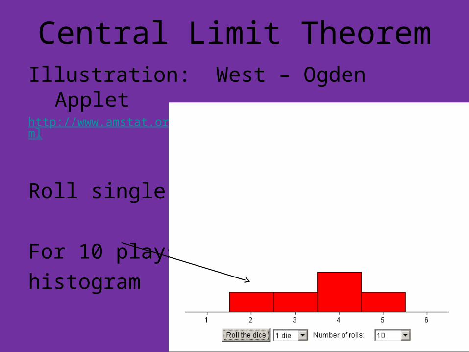
Central Limit TheoremIllustration: West – Ogden Applethttp://www.amstat.org/publications/jse/v6n3/applets/CLT.html
Roll single die
For 10 plays,
histogram
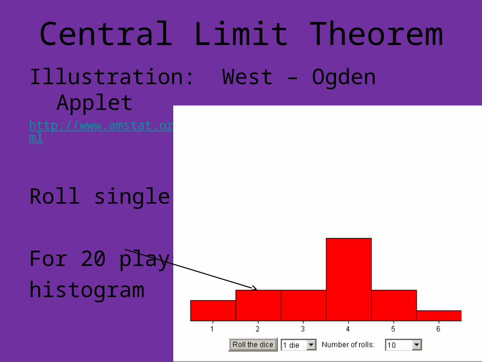
Central Limit TheoremIllustration: West – Ogden Applethttp://www.amstat.org/publications/jse/v6n3/applets/CLT.html
Roll single die
For 20 plays,
histogram
Central Limit TheoremIllustration: West – Ogden Applethttp://www.amstat.org/publications/jse/v6n3/applets/CLT.html
Roll single die
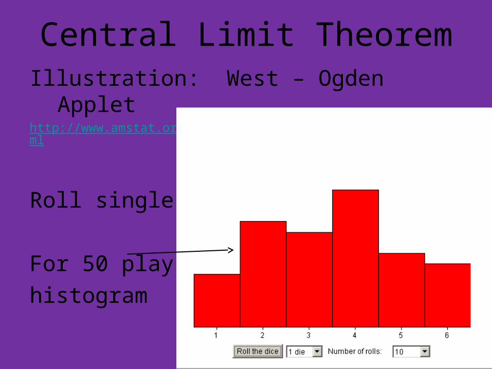
For 50 plays,
histogram
Central Limit TheoremIllustration: West – Ogden Applethttp://www.amstat.org/publications/jse/v6n3/applets/CLT.html
Roll single die
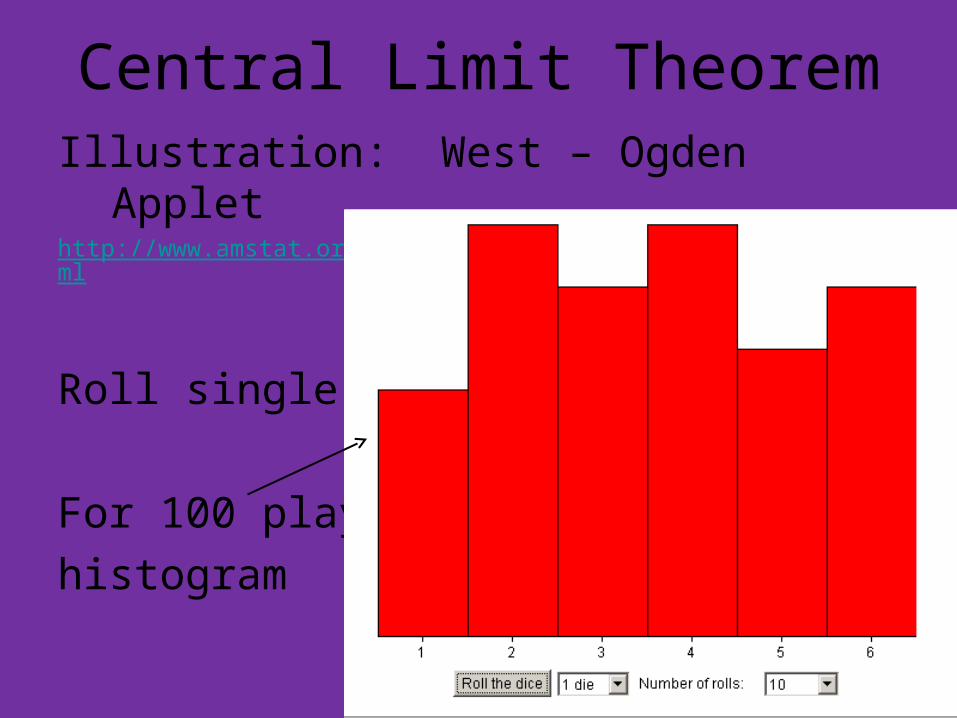
For 100 plays,
histogram

Central Limit TheoremIllustration: West – Ogden Applethttp://www.amstat.org/publications/jse/v6n3/applets/CLT.html
Roll single die
For 1000 plays,
histogram

Central Limit TheoremIllustration: West – Ogden Applethttp://www.amstat.org/publications/jse/v6n3/applets/CLT.html
Roll single die
For 10,000 plays,
histogram

Central Limit TheoremIllustration: West – Ogden Applethttp://www.amstat.org/publications/jse/v6n3/applets/CLT.html
Roll single die
For 100,000 plays,
histogram
Stabilizes at
Uniform
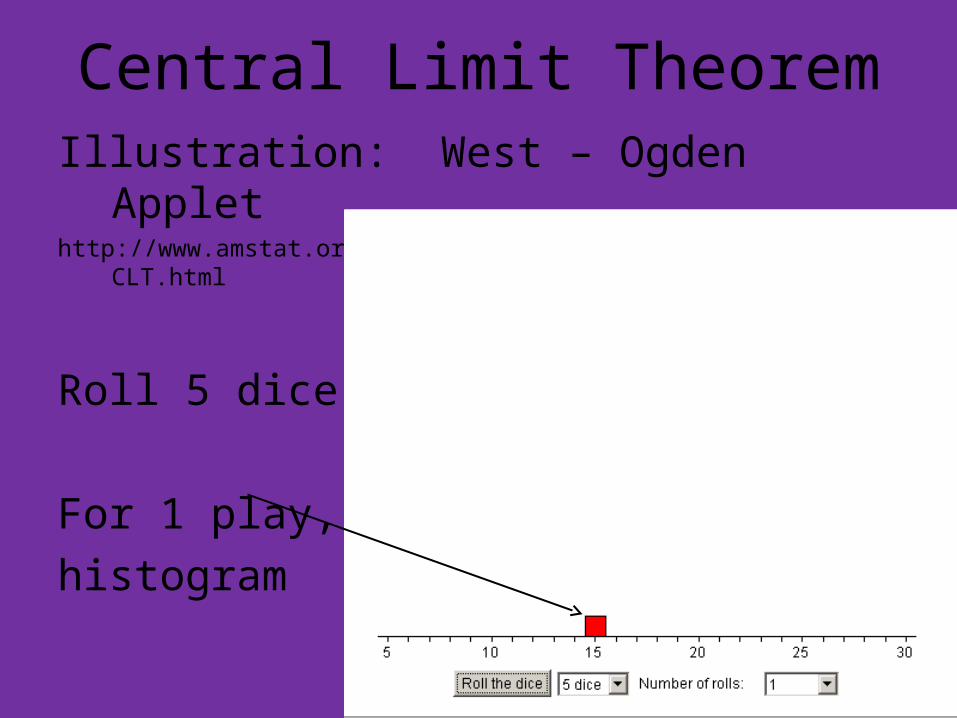
Central Limit TheoremIllustration: West – Ogden Applethttp://www.amstat.org/publications/jse/v6n3/applets/CLT.html
Roll 5 dice
For 1 play,
histogram

Central Limit TheoremIllustration: West – Ogden Applethttp://www.amstat.org/publications/jse/v6n3/applets/CLT.html
Roll 5 dice
For 10 plays,
histogram

Central Limit TheoremIllustration: West – Ogden Applethttp://www.amstat.org/publications/jse/v6n3/applets/CLT.html
Roll 5 dice
For 100 plays,
histogram

Central Limit TheoremIllustration: West – Ogden Applethttp://www.amstat.org/publications/jse/v6n3/applets/CLT.html
Roll 5 dice
For 1000 plays,
histogram

Central Limit TheoremIllustration: West – Ogden Applethttp://www.amstat.org/publications/jse/v6n3/applets/CLT.html
Roll 5 dice
For 10,000 plays,
histogram
Looks mound
shaped

Central Limit TheoremFor any random sample
and for n “large”
is “roughly”
Some nice illustrations:
• Applet by Webster West & Todd Ogden
• Applet from Rice Univ.
nXX ,,1
X ,N

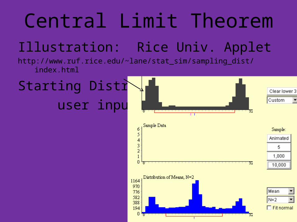
Central Limit TheoremIllustration: Rice Univ. Applethttp://www.ruf.rice.edu/~lane/stat_sim/sampling_dist/index.html
Starting Distribut’n
Central Limit TheoremIllustration: Rice Univ. Applethttp://www.ruf.rice.edu/~lane/stat_sim/sampling_dist/index.html
Starting Distribut’n
user input

Central Limit TheoremIllustration: Rice Univ. Applethttp://www.ruf.rice.edu/~lane/stat_sim/sampling_dist/index.html
Starting Distribut’n
user input
(very non-Normal)

Central Limit TheoremIllustration: Rice Univ. Applethttp://www.ruf.rice.edu/~lane/stat_sim/sampling_dist/index.html
Starting Distribut’n
user input
(very non-Normal)
Dist’n of average
of n = 2

Central Limit TheoremIllustration: Rice Univ. Applethttp://www.ruf.rice.edu/~lane/stat_sim/sampling_dist/index.html
Starting Distribut’n
user input
(very non-Normal)
Dist’n of average
of n = 2
(slightly more
mound shaped?)

Central Limit TheoremIllustration: Rice Univ. Applethttp://www.ruf.rice.edu/~lane/stat_sim/sampling_dist/index.html
Starting Distribut’n
user input
(very non-Normal)
Dist’n of average
of n = 5
(little more
mound shaped?)

Central Limit TheoremIllustration: Rice Univ. Applethttp://www.ruf.rice.edu/~lane/stat_sim/sampling_dist/index.html
Starting Distribut’n
user input
(very non-Normal)
Dist’n of average
of n = 10
(much more
mound shaped?)
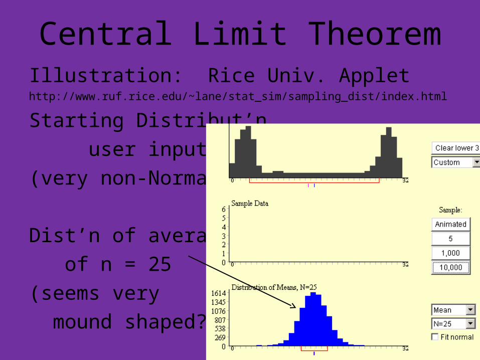
Central Limit TheoremIllustration: Rice Univ. Applethttp://www.ruf.rice.edu/~lane/stat_sim/sampling_dist/index.html
Starting Distribut’n
user input
(very non-Normal)
Dist’n of average
of n = 25
(seems very
mound shaped?)

Central Limit TheoremFor any random sample
and for n “large”
is “roughly”
Some nice illustrations:
• Applet by Webster West & Todd Ogden
• Applet from Rice Univ.
• Stats Portal Applet
nXX ,,1
X ,N

Central Limit TheoremIllustration: StatsPortal. Applet
http://courses.bfwpub.com/ips6e
Density for average
of n = 1, from
Exponential dist’n

Central Limit TheoremIllustration: StatsPortal. Applet
http://courses.bfwpub.com/ips6e
Density for average
of n = 1, from
Exponential dist’n
Best fit Normal
density

Central Limit TheoremIllustration: StatsPortal. Applet
http://courses.bfwpub.com/ips6e
Density for average
of n = 2, from
Exponential dist’n
Best fit Normal
density

Central Limit TheoremIllustration: StatsPortal. Applet
http://courses.bfwpub.com/ips6e
Density for average
of n = 4, from
Exponential dist’n
Best fit Normal
density

Central Limit TheoremIllustration: StatsPortal. Applet
http://courses.bfwpub.com/ips6e
Density for average
of n = 10, from
Exponential dist’n
Best fit Normal
density

Central Limit TheoremIllustration: StatsPortal. Applet
http://courses.bfwpub.com/ips6e
Density for average
of n = 30, from
Exponential dist’n
Best fit Normal
density

Central Limit TheoremIllustration: StatsPortal. Applet
http://courses.bfwpub.com/ips6e
Density for average
of n = 100, from
Exponential dist’n
Best fit Normal
density

Central Limit TheoremIllustration: StatsPortal. Applet
http://courses.bfwpub.com/ips6e
Very strong
Convergence
For n = 100

Central Limit TheoremIllustration: StatsPortal. Applet
http://courses.bfwpub.com/ips6e
Looks “pretty good”
For n = 30

Central Limit TheoremFor any random sample
and for n “large”
is “roughly”
How large n is needed?
nXX ,,1
X ,N

Central Limit TheoremHow large n is needed?

Central Limit TheoremHow large n is needed?
• Depends completely on setup
Central Limit TheoremHow large n is needed?
• Depends completely on setup
• Indiv. obs. Close to normal small OK

Central Limit TheoremHow large n is needed?
• Depends completely on setup
• Indiv. obs. Close to normal small OK
• But can be large in extreme cases

Central Limit TheoremHow large n is needed?
• Depends completely on setup
• Indiv. obs. Close to normal small OK
• But can be large in extreme cases
• Many people “often feel good”,
when n ≥ 30
Central Limit TheoremHow large n is needed?
• Depends completely on setup
• Indiv. obs. Close to normal small OK
• But can be large in extreme cases
• Many people “often feel good”,
when n ≥ 30
Review earlier examples

Central Limit TheoremIllustration: Rice Univ. Applethttp://www.ruf.rice.edu/~lane/stat_sim/sampling_dist/index.html
Starting Distribut’n
user input
(very non-Normal)
Dist’n of average
of n = 25
(seems very
mound shaped?)

Central Limit TheoremIllustration: StatsPortal. Applet
http://courses.bfwpub.com/ips6e
Looks “pretty good”
For n = 30

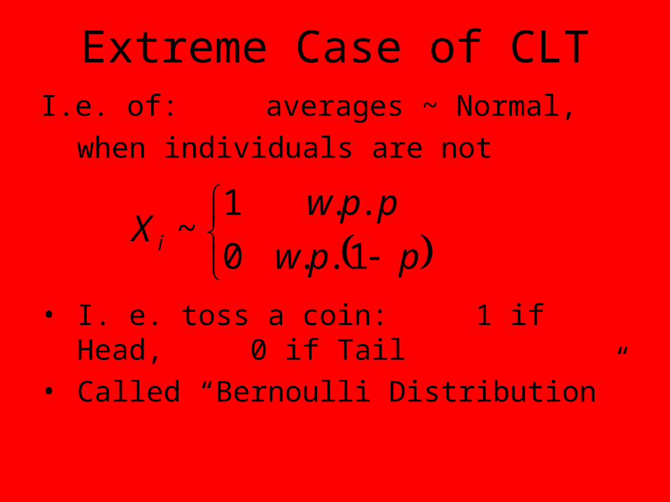
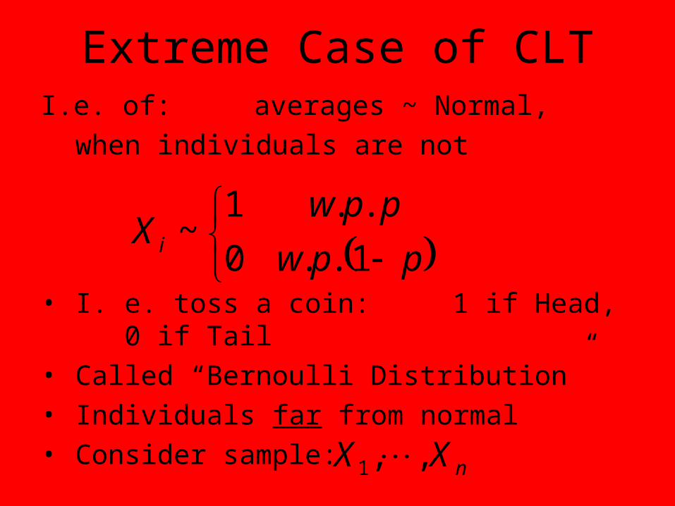
Extreme Case of CLTI.e. of: averages ~ Normal,
when individuals are not

Extreme Case of CLTI.e. of: averages ~ Normal,
when individuals are not

Extreme Case of CLTI.e. of: averages ~ Normal,
when individuals are not
ppw
ppwX i 1..0
..1~

Extreme Case of CLTI.e. of: averages ~ Normal,
when individuals are not
• I. e. toss a coin: 1 if Head, 0 if Tail
ppw
ppwX i 1..0
..1~
Extreme Case of CLTI.e. of: averages ~ Normal,
when individuals are not
• I. e. toss a coin: 1 if Head, 0 if Tail
• Called “Bernoulli Distribution”
ppw
ppwX i 1..0
..1~
Extreme Case of CLTI.e. of: averages ~ Normal,
when individuals are not
• I. e. toss a coin: 1 if Head, 0 if Tail
• Called “Bernoulli Distribution”
• Individuals far from normal
• Consider sample:
ppw
ppwX i 1..0
..1~
nXX ,,1

Extreme Case of CLTBernoulli sample: nXX ,,1

Extreme Case of CLTBernoulli sample:
(Recall: independent,
with same distribution)
nXX ,,1

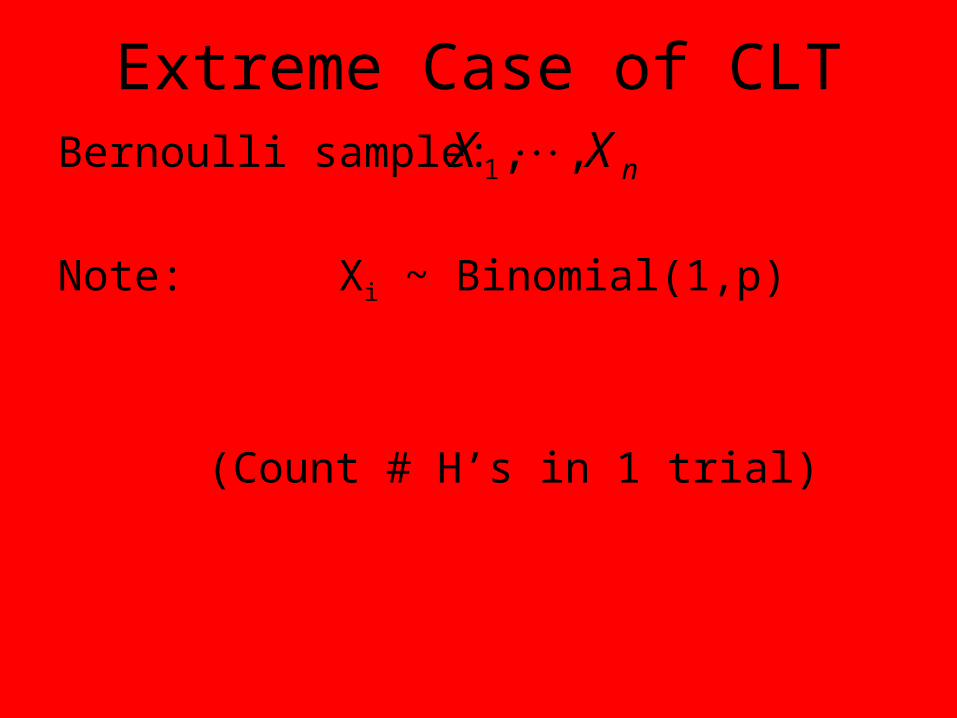
Extreme Case of CLTBernoulli sample:
Note: Xi ~ Binomial(1,p)
nXX ,,1
Extreme Case of CLTBernoulli sample:
Note: Xi ~ Binomial(1,p)
(Count # H’s in 1 trial)
nXX ,,1

Extreme Case of CLTBernoulli sample:
Note: Xi ~ Binomial(1,p)
So:
EXi = p
nXX ,,1

Extreme Case of CLTBernoulli sample:
Note: Xi ~ Binomial(1,p)
So:
EXi = p
Recall np, with p = 1
nXX ,,1

Extreme Case of CLTBernoulli sample:
Note: Xi ~ Binomial(1,p)
So:
EXi = p
var(Xi) = p(1-p)
nXX ,,1

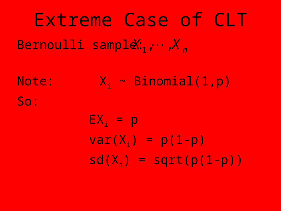
Extreme Case of CLTBernoulli sample:
Note: Xi ~ Binomial(1,p)
So:
EXi = p
var(Xi) = p(1-p)
Recall np(1-p), with p = 1
nXX ,,1
Extreme Case of CLTBernoulli sample:
Note: Xi ~ Binomial(1,p)
So:
EXi = p
var(Xi) = p(1-p)
sd(Xi) = sqrt(p(1-p))
nXX ,,1

Extreme Case of CLTBernoulli sample:
EXi = p
sd(Xi) = sqrt(p(1-p))
nXX ,,1

Extreme Case of CLTBernoulli sample:
EXi = p
sd(Xi) = sqrt(p(1-p))
So Law of Averages
nXX ,,1
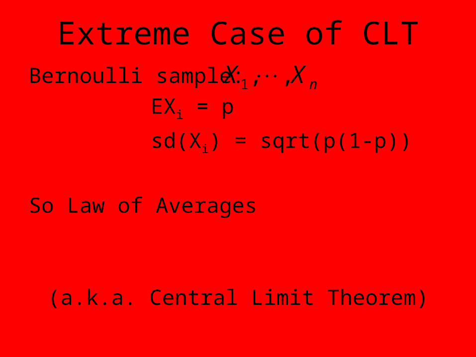
Extreme Case of CLTBernoulli sample:
EXi = p
sd(Xi) = sqrt(p(1-p))
So Law of Averages
(a.k.a. Central Limit Theorem)
nXX ,,1

Extreme Case of CLTBernoulli sample:
EXi = p
sd(Xi) = sqrt(p(1-p))
So Law of Averages gives:
roughly
nXX ,,1
X npppN 1,

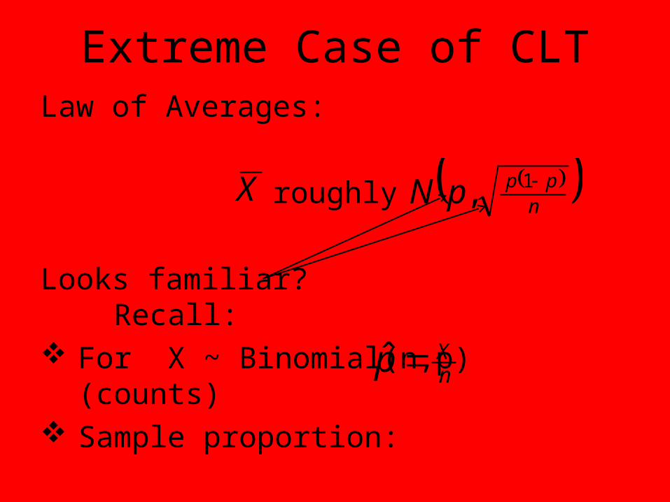
Extreme Case of CLTLaw of Averages:
roughlyX npppN 1,

Extreme Case of CLTLaw of Averages:
roughly
Looks familiar?
X npppN 1,

Extreme Case of CLTLaw of Averages:
roughly
Looks familiar? Recall: For X ~ Binomial(n,p) (counts)
X npppN 1,
Extreme Case of CLTLaw of Averages:
roughly
Looks familiar? Recall: For X ~ Binomial(n,p) (counts) Sample proportion:
X npppN 1,
nXp ˆ

Extreme Case of CLTLaw of Averages:
roughly
Looks familiar? Recall: For X ~ Binomial(n,p) (counts) Sample proportion: Has: &
X npppN 1,
nXp ˆ
pEpE nX ˆ
npppsd 1ˆ

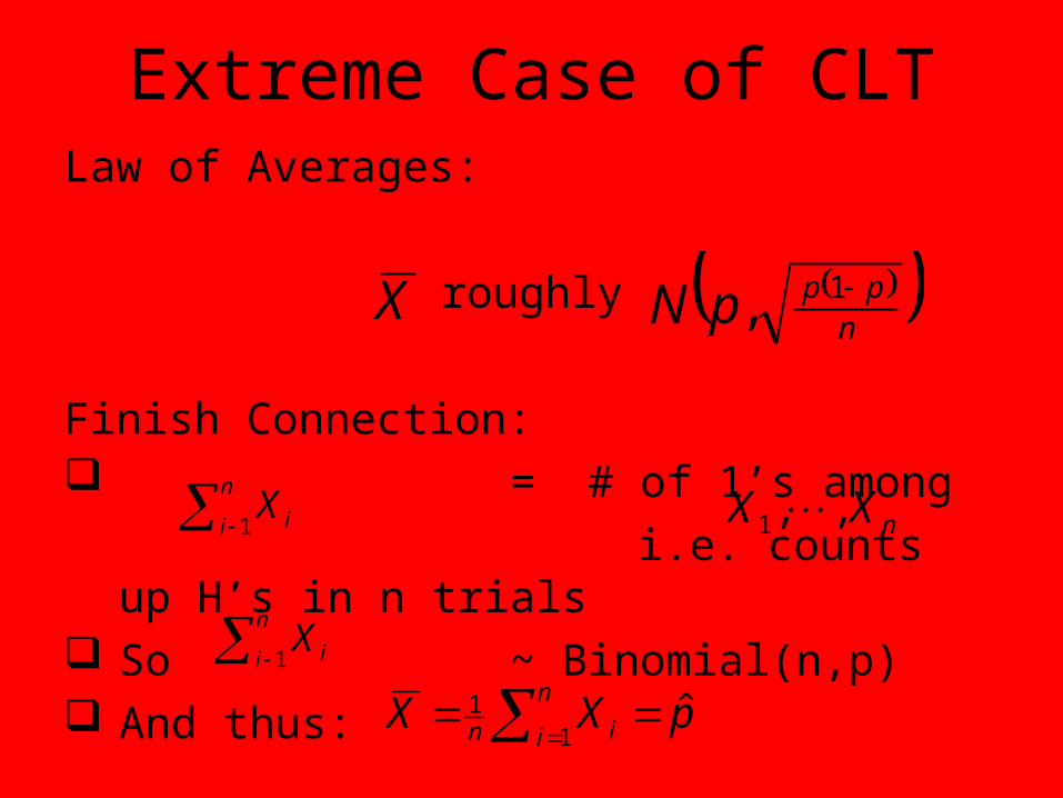
Extreme Case of CLTLaw of Averages:
roughly
Finish Connection:
X npppN 1,
Extreme Case of CLTLaw of Averages:
roughly
Finish Connection: = # of 1’s among
i.e. counts up H’s in n trials So ~ Binomial(n,p) And thus:
X npppN 1,
nXX ,,1
n
i iX1
n
i iX1
pXXn
i inˆ
11

Extreme Case of CLTLaw of Averages:
roughly
Finish Connection: = # of 1’s among
i.e. counts up H’s in n trials So ~ Binomial(n,p) And thus:
X npppN 1,
nXX ,,1
n
i iX1
n
i iX1
pXXn
i inˆ
11

Extreme Case of CLTConsequences:
roughlyp npppN 1,

Extreme Case of CLTConsequences:
roughly
roughly
p npppN 1,
X pnpnpN 1,

Extreme Case of CLTConsequences:
roughly
roughly
(using and
multiply through by n)
p npppN 1,
X pnpnpN 1,
nXp ˆ

Extreme Case of CLTConsequences:
roughly
roughly
Terminology: Called
The Normal Approximation to the Binomial
p npppN 1,
X pnpnpN 1,

Extreme Case of CLTConsequences:
roughly
roughly
Terminology: Called
The Normal Approximation to the Binomial
p npppN 1,
X pnpnpN 1,

Extreme Case of CLTConsequences:
roughly
roughly
Terminology: Called
The Normal Approximation to the Binomial
(and the sample proportion case)
p npppN 1,
X pnpnpN 1,

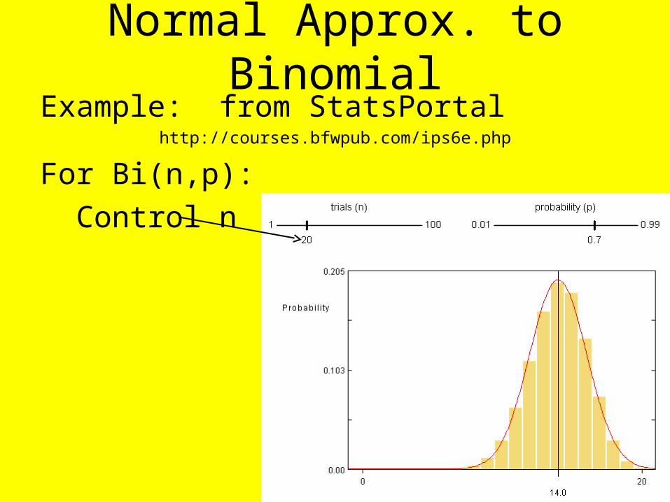
Normal Approx. to BinomialExample: from StatsPortal
http://courses.bfwpub.com/ips6e.php
Normal Approx. to BinomialExample: from StatsPortal
http://courses.bfwpub.com/ips6e.php
For Bi(n,p):
Control n

Normal Approx. to BinomialExample: from StatsPortal
http://courses.bfwpub.com/ips6e.php
For Bi(n,p):
Control n
Control p

Normal Approx. to BinomialExample: from StatsPortal
http://courses.bfwpub.com/ips6e.php
For Bi(n,p):
Control n
Control p
See Prob. Histo.
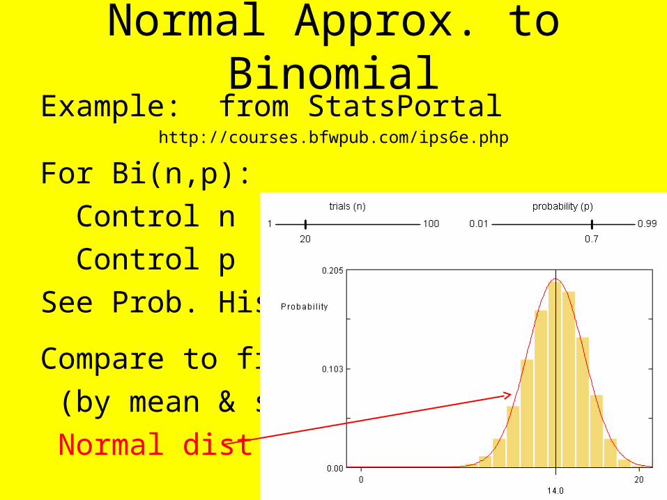
Normal Approx. to BinomialExample: from StatsPortal
http://courses.bfwpub.com/ips6e.php
For Bi(n,p):
Control n
Control p
See Prob. Histo.
Compare to fit
(by mean & sd)
Normal dist’n

Normal Approx. to BinomialExample: from StatsPortal
http://courses.bfwpub.com/ips6e.php
For Bi(n,p):
n = 20
p = 0.5
Expect:
20*0.5 = 10
(most likely)

Normal Approx. to BinomialExample: from StatsPortal
http://courses.bfwpub.com/ips6e.php
For Bi(n,p):
n = 20
p = 0.5
Reasonable
Normal fit

Normal Approx. to BinomialExample: from StatsPortal
http://courses.bfwpub.com/ips6e.php
For Bi(n,p):
n = 20
p = 0.2
Expect:
20*0.2 = 4
(most likely)
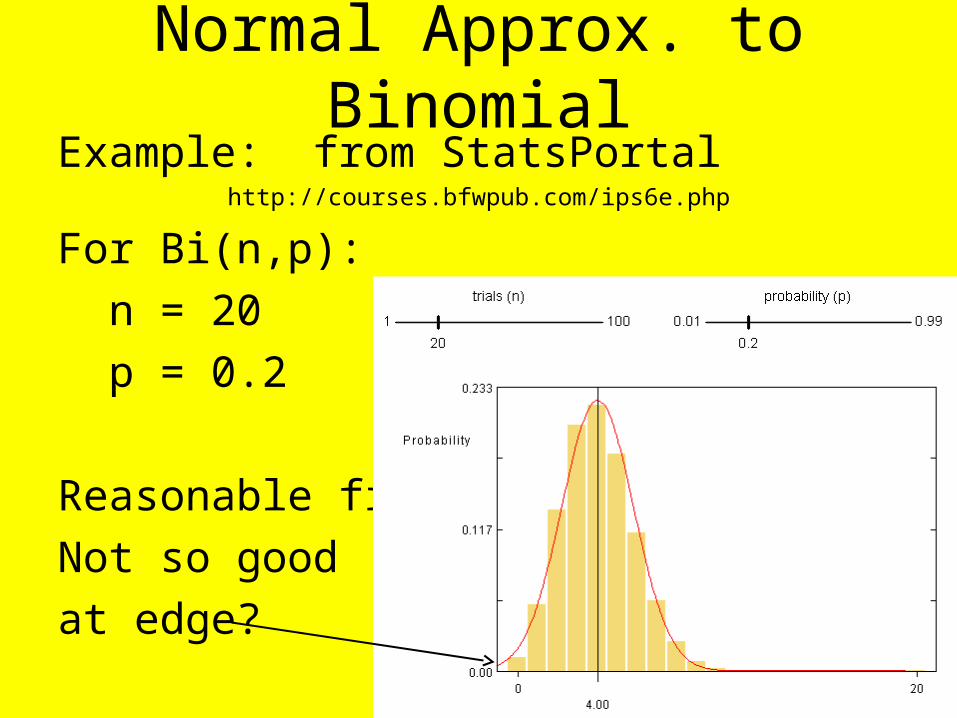
Normal Approx. to BinomialExample: from StatsPortal
http://courses.bfwpub.com/ips6e.php
For Bi(n,p):
n = 20
p = 0.2
Reasonable fit?
Not so good
at edge?

Normal Approx. to BinomialExample: from StatsPortal
http://courses.bfwpub.com/ips6e.php
For Bi(n,p):
n = 20
p = 0.1
Expect:
20*0.1 = 2
(most likely)
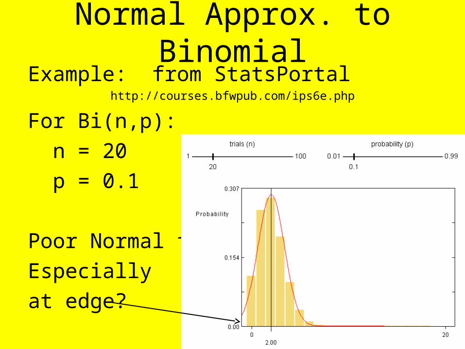
Normal Approx. to BinomialExample: from StatsPortal
http://courses.bfwpub.com/ips6e.php
For Bi(n,p):
n = 20
p = 0.1
Poor Normal fit,
Especially
at edge?

Normal Approx. to BinomialExample: from StatsPortal
http://courses.bfwpub.com/ips6e.php
For Bi(n,p):
n = 20
p = 0.05
Expect:
20*0.05 = 1
(most likely)
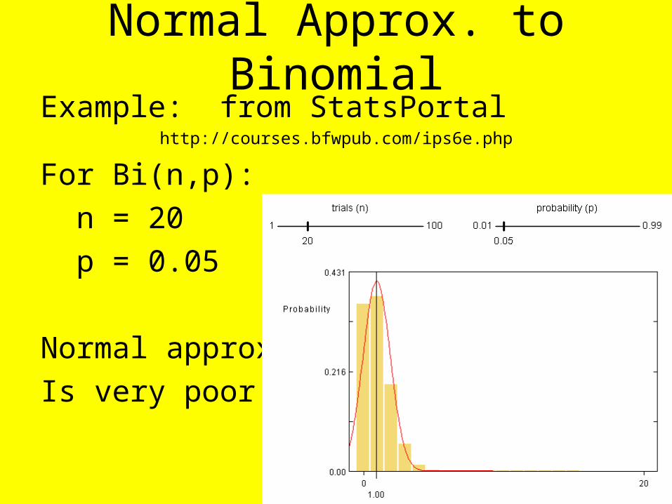
Normal Approx. to BinomialExample: from StatsPortal
http://courses.bfwpub.com/ips6e.php
For Bi(n,p):
n = 20
p = 0.05
Normal approx
Is very poor
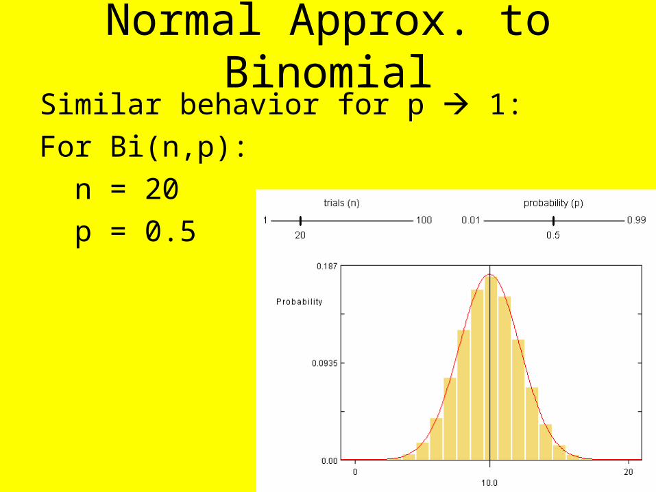
Normal Approx. to BinomialSimilar behavior for p 1:
For Bi(n,p):
n = 20
p = 0.5
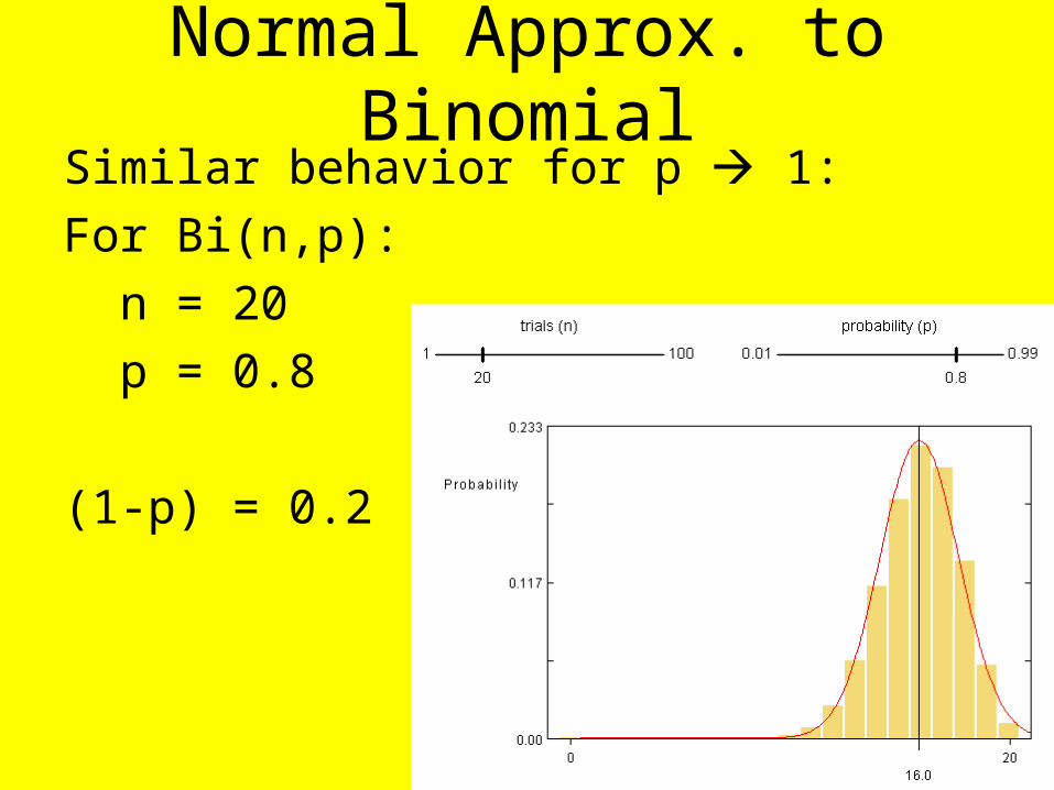
Normal Approx. to BinomialSimilar behavior for p 1:
For Bi(n,p):
n = 20
p = 0.8
(1-p) = 0.2
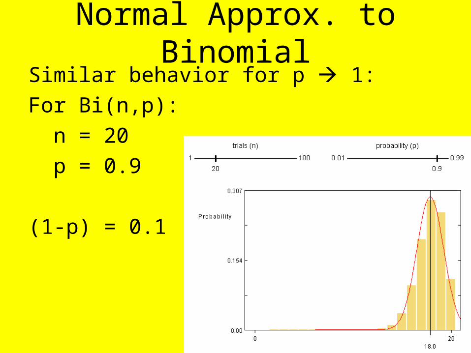
Normal Approx. to BinomialSimilar behavior for p 1:
For Bi(n,p):
n = 20
p = 0.9
(1-p) = 0.1

Normal Approx. to BinomialSimilar behavior for p 1:
For Bi(n,p):
n = 20
p = 0.95
(1-p) = 0.05
Mirror image
of above

Normal Approx. to BinomialNow fix p, and let n vary:
For Bi(n,p):
n = 1
p = 0.3

Normal Approx. to BinomialNow fix p, and let n vary:
For Bi(n,p):
n = 3
p = 0.3

Normal Approx. to BinomialNow fix p, and let n vary:
For Bi(n,p):
n = 10
p = 0.3

Normal Approx. to BinomialNow fix p, and let n vary:
For Bi(n,p):
n = 30
p = 0.3
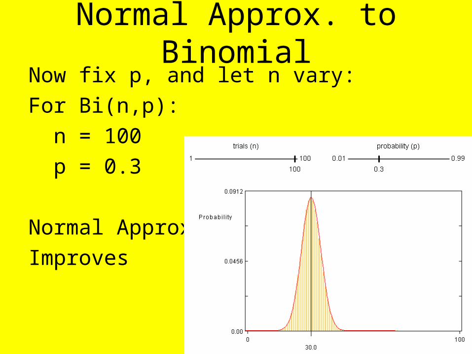
Normal Approx. to BinomialNow fix p, and let n vary:
For Bi(n,p):
n = 100
p = 0.3
Normal Approx.
Improves
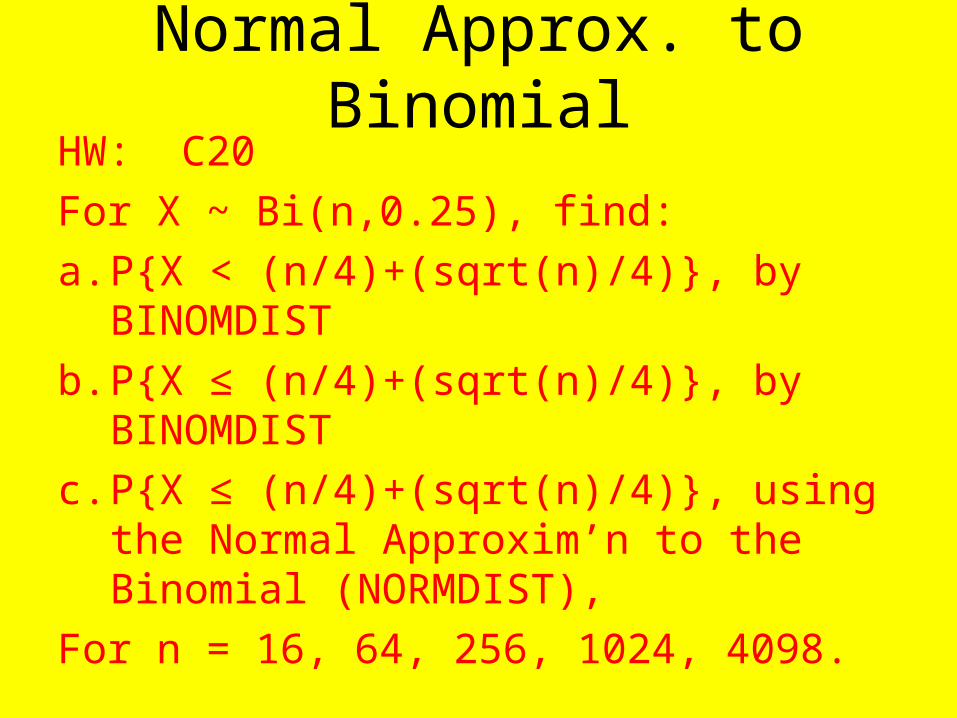
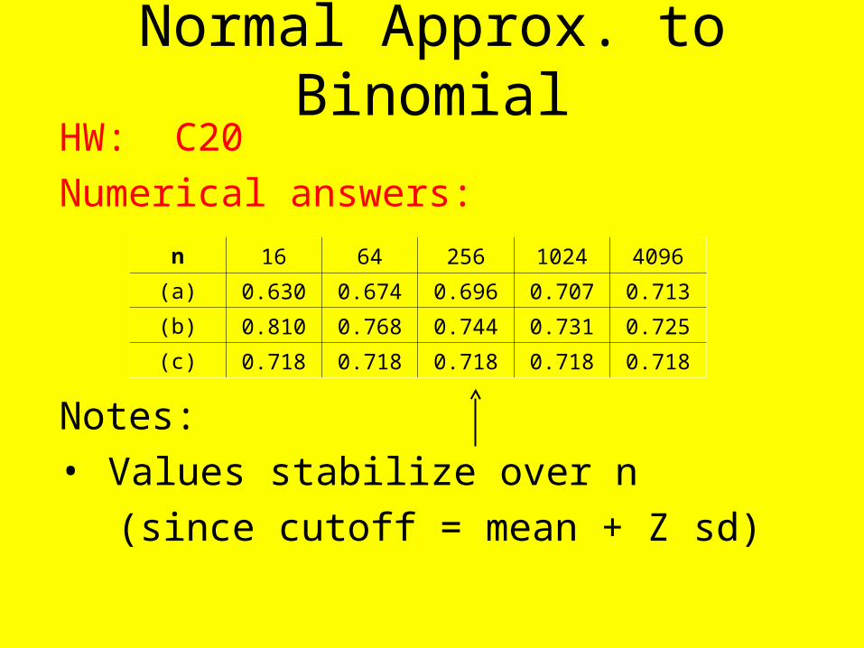
Normal Approx. to BinomialHW: C20
For X ~ Bi(n,0.25), find:
a. P{X < (n/4)+(sqrt(n)/4)}, by BINOMDIST
b. P{X ≤ (n/4)+(sqrt(n)/4)}, by BINOMDIST
c. P{X ≤ (n/4)+(sqrt(n)/4)}, using the Normal Approxim’n to the Binomial (NORMDIST),
For n = 16, 64, 256, 1024, 4098.

Normal Approx. to BinomialHW: C20
Numerical answers:
n 16 64 256 1024 4096
(a) 0.630 0.674 0.696 0.707 0.713
(b) 0.810 0.768 0.744 0.731 0.725
(c) 0.718 0.718 0.718 0.718 0.718
Normal Approx. to BinomialHW: C20
Numerical answers:
Notes:
• Values stabilize over n
(since cutoff = mean + Z sd)
n 16 64 256 1024 4096
(a) 0.630 0.674 0.696 0.707 0.713
(b) 0.810 0.768 0.744 0.731 0.725
(c) 0.718 0.718 0.718 0.718 0.718

Normal Approx. to BinomialHW: C20
Numerical answers:
Notes:
• Values stabilize over n
• Normal approx. between others
• Everything close for larger n
n 16 64 256 1024 4096
(a) 0.630 0.674 0.696 0.707 0.713
(b) 0.810 0.768 0.744 0.731 0.725
(c) 0.718 0.718 0.718 0.718 0.718

Normal Approx. to BinomialHW: C20
Numerical answers:
Notes:
• Values stabilize over n
• Normal approx. between others
n 16 64 256 1024 4096
(a) 0.630 0.674 0.696 0.707 0.713
(b) 0.810 0.768 0.744 0.731 0.725
(c) 0.718 0.718 0.718 0.718 0.718

Normal Approx. to BinomialHW: C20
Numerical answers:
Notes:
• Values stabilize over n
• Normal approx. between others
n 16 64 256 1024 4096
(a) 0.630 0.674 0.696 0.707 0.713
(b) 0.810 0.768 0.744 0.731 0.725
(c) 0.718 0.718 0.718 0.718 0.718
Normal Approx. to BinomialHow large n?

Normal Approx. to BinomialHow large n?
• Bigger is better
Normal Approx. to BinomialHow large n?
• Bigger is better
• Could use “n ≥ 30” rule from above
Law of Averages

Normal Approx. to BinomialHow large n?
• Bigger is better
• Could use “n ≥ 30” rule from above
Law of Averages
• But clearly depends on p

Normal Approx. to BinomialHow large n?
• Bigger is better
• Could use “n ≥ 30” rule from above
Law of Averages
• But clearly depends on p– Worse for p ≈ 0

Normal Approx. to BinomialHow large n?
• Bigger is better
• Could use “n ≥ 30” rule from above
Law of Averages
• But clearly depends on p– Worse for p ≈ 0– And for p ≈ 1

Normal Approx. to BinomialHow large n?
• Bigger is better
• Could use “n ≥ 30” rule from above
Law of Averages
• But clearly depends on p– Worse for p ≈ 0– And for p ≈ 1– i.e. (1 – p) ≈ 0

Normal Approx. to BinomialHow large n?
• Bigger is better
• Could use “n ≥ 30” rule from above
Law of Averages
• But clearly depends on p
• Textbook Rule:
OK when {np ≥ 10 & n(1-p) ≥ 10}

Normal Approx. to BinomialHW: 5.18 (a. population too small, b. np =
2 < 10)
C21: Which binomial distributions admit a “good” normal approximation?
a. Bi(30, 0.3)
b. Bi(40, 0.4)
c. Bi(20,0.5)
d. Bi(30,0.7)
(no, yes, yes, no)

And now for somethingcompletely different….
A statistics professor was describing
sampling theory to his class, explaining
how a sample can be studied and used
to generalize to a population.
One of the students in the back of the room
kept shaking his head.
And now for somethingcompletely different….
"What's the matter?" asked the professor.
"I don't believe it," said the student, "why not study the whole population in the first place?"
The professor continued explaining the ideas of random and representative samples.
The student still shook his head.

And now for somethingcompletely different….
The professor launched into the mechanics of
proportional stratified samples, randomized
cluster sampling, the standard error of the
mean, and the central limit theorem.
The student remained unconvinced saying, "Too
much theory, too risky, I couldn't trust just a
few numbers in place of ALL of them."

And now for somethingcompletely different….
Attempting a more practical example, the professor then explained the scientific rigor and meticulous sample selection of the Nielsen television ratings which are used to determine how multiple millions of advertising dollars are spent.
The student remained unimpressed saying, "You mean that just a sample of a few thousand can tell us exactly what over 250 MILLION people are doing?"

And now for somethingcompletely different….
Finally, the professor, somewhat disgruntled with the skepticism, replied,
"Well, the next time you go to the campus clinic and they want to do a blood test...tell them that's not good enough ...
tell them to TAKE IT ALL!!"
From: GARY C. RAMSEYER• http://www.ilstu.edu/~gcramsey/Gallery.html
Central Limit TheoremFurther Consequences of Law of Averages:
Central Limit TheoremFurther Consequences of Law of Averages:
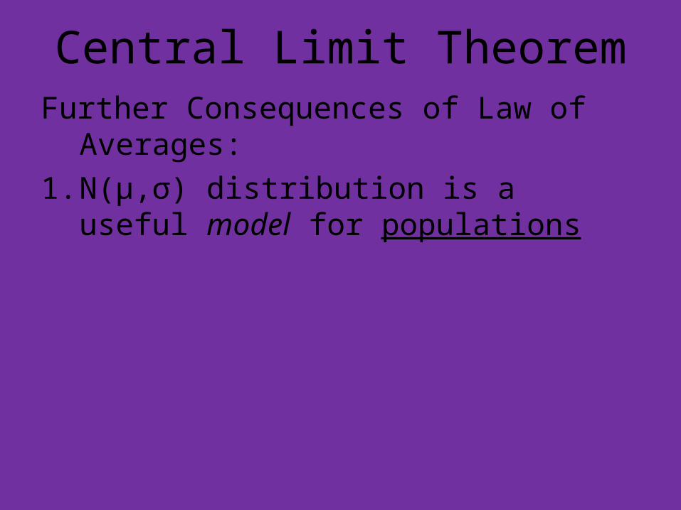
1. N(μ,σ) distribution is a useful model for populations

Central Limit TheoremFurther Consequences of Law of Averages:
1. N(μ,σ) distribution is a useful model for populations
e.g. SAT scores are averages of scores from many questions

Central Limit TheoremFurther Consequences of Law of Averages:
1. N(μ,σ) distribution is a useful model for populations
e.g. SAT scores are averages of scores from many questions
e.g. heights are influenced by many small factors, your height is sum of these.

Central Limit TheoremFurther Consequences of Law of Averages:
1. N(μ,σ) distribution is a useful model for populations
e.g. SAT scores are averages of scores from many questions
e.g. heights are influenced by many small factors, your height is sum of these.
2. N(μ,σ) distribution useful for modeling measurement error
Sum of many small components

Central Limit TheoremFurther Consequences of Law of Averages:
1. N(μ,σ) distribution is a useful model for populations
2. N(μ,σ) distribution useful for modeling measurement error

Central Limit TheoremFurther Consequences of Law of Averages:
1. N(μ,σ) distribution is a useful model for populations
2. N(μ,σ) distribution useful for modeling measurement error
Now have powerful probability tools for
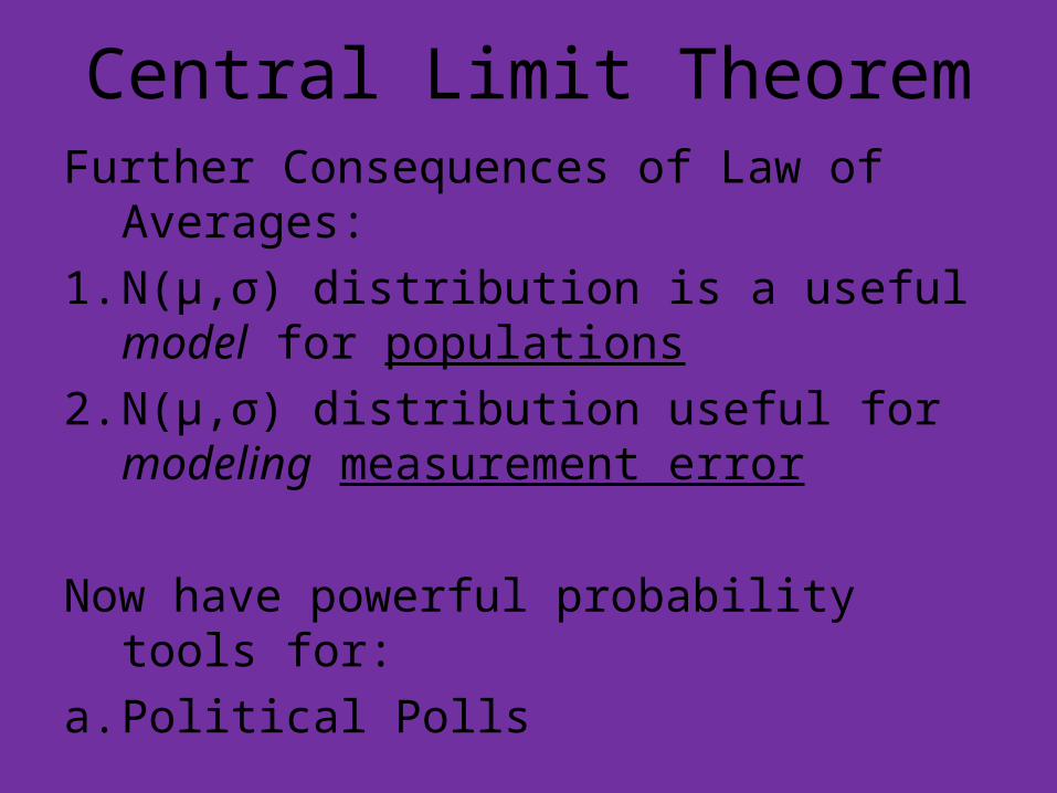
Central Limit TheoremFurther Consequences of Law of Averages:
1. N(μ,σ) distribution is a useful model for populations
2. N(μ,σ) distribution useful for modeling measurement error
Now have powerful probability tools for:
a. Political Polls

Central Limit TheoremFurther Consequences of Law of Averages:
1. N(μ,σ) distribution is a useful model for populations
2. N(μ,σ) distribution useful for modeling measurement error
Now have powerful probability tools for:
a. Political Polls
b. Populations – Measurement Error

Course Big PictureNow have powerful probability tools for:
a. Political Polls
b. Populations – Measurement Error

Course Big PictureNow have powerful probability tools for:
a. Political Polls
b. Populations – Measurement Error
Next deal systematically with unknown p & μ

Course Big PictureNow have powerful probability tools for:
a. Political Polls
b. Populations – Measurement Error
Next deal systematically with unknown p & μ
Subject called “Statistical Inference”

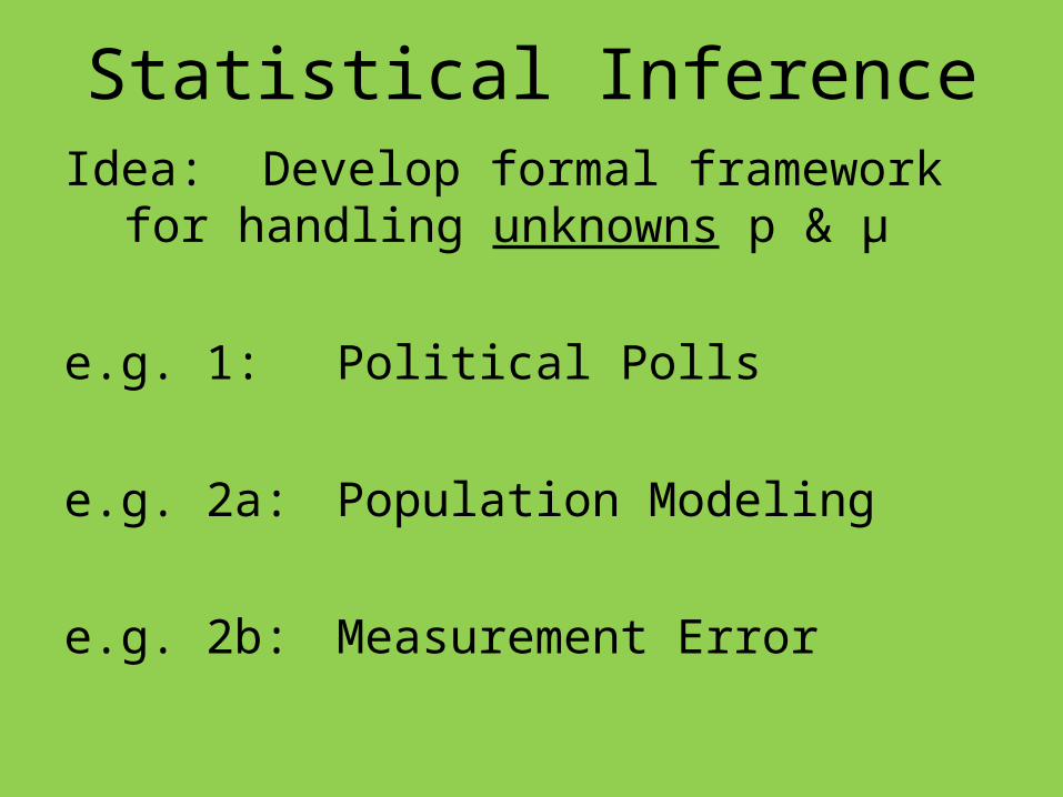
Statistical InferenceIdea: Develop formal framework for
handling unknowns p & μ
Statistical InferenceIdea: Develop formal framework for
handling unknowns p & μ
(major work for this is already done)

Statistical InferenceIdea: Develop formal framework for
handling unknowns p & μ
(major work for this is already done)
(now will just formalize, and refine)

Statistical InferenceIdea: Develop formal framework for
handling unknowns p & μ
(major work for this is already done)
(now will just formalize, and refine)
(do for simultaneously for major models)

Statistical InferenceIdea: Develop formal framework for
handling unknowns p & μ
e.g. 1: Political Polls

Statistical InferenceIdea: Develop formal framework for
handling unknowns p & μ
e.g. 1: Political Polls
(estimate p = proportion for A)

Statistical InferenceIdea: Develop formal framework for
handling unknowns p & μ
e.g. 1: Political Polls
(estimate p = proportion for A)
(in population, based on sample)

Statistical InferenceIdea: Develop formal framework for
handling unknowns p & μ
e.g. 1: Political Polls
e.g. 2a: Population Modeling

Statistical InferenceIdea: Develop formal framework for
handling unknowns p & μ
e.g. 1: Political Polls
e.g. 2a: Population Modeling
(e.g. heights, SAT scores …)
Statistical InferenceIdea: Develop formal framework for
handling unknowns p & μ
e.g. 1: Political Polls
e.g. 2a: Population Modeling
e.g. 2b: Measurement Error

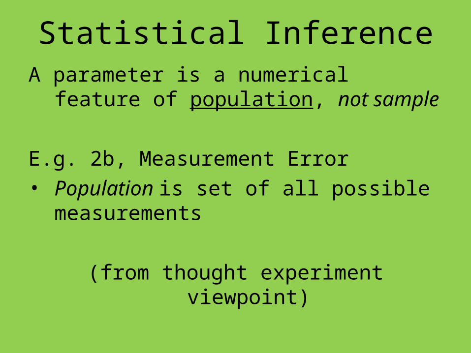
Statistical InferenceA parameter is a numerical feature
Statistical InferenceA parameter is a numerical feature of
population

Statistical InferenceA parameter is a numerical feature of
population, not sample

Statistical InferenceA parameter is a numerical feature of
population, not sample
(so far parameters have been indices
of probability distributions)

Statistical InferenceA parameter is a numerical feature of
population, not sample
(so far parameters have been indices
of probability distributions)
(this is an additional role for that term)
Statistical InferenceA parameter is a numerical feature of
population, not sample
E.g. 1, Political Polls
• Population is all voters

Statistical InferenceA parameter is a numerical feature of
population, not sample
E.g. 1, Political Polls
• Population is all voters
• Parameter is proportion of population for A

Statistical InferenceA parameter is a numerical feature of
population, not sample
E.g. 1, Political Polls
• Population is all voters
• Parameter is proportion of population for A, often denoted by p

Statistical InferenceA parameter is a numerical feature of
population, not sample
E.g. 1, Political Polls
• Population is all voters
• Parameter is proportion of population for A, often denoted by p
(same as p before, just new framework)

Statistical InferenceA parameter is a numerical feature of
population, not sample
E.g. 2a, Population Modeling
• Parameters are μ & σ

Statistical InferenceA parameter is a numerical feature of
population, not sample
E.g. 2a, Population Modeling
• Parameters are μ & σ
(population mean & sd)
Statistical InferenceA parameter is a numerical feature of
population, not sample
E.g. 2b, Measurement Error
• Population is set of all possible measurements
Statistical InferenceA parameter is a numerical feature of
population, not sample
E.g. 2b, Measurement Error
• Population is set of all possible measurements
(from thought experiment viewpoint)

Statistical InferenceA parameter is a numerical feature of
population, not sample
E.g. 2b, Measurement Error
• Population is set of all possible measurements
• Parameters are

Statistical InferenceA parameter is a numerical feature of
population, not sample
E.g. 2b, Measurement Error
• Population is set of all possible measurements
• Parameters are:– μ = true value

Statistical InferenceA parameter is a numerical feature of
population, not sample
E.g. 2b, Measurement Error
• Population is set of all possible measurements
• Parameters are:– μ = true value– σ = s.d. of measurements

Statistical InferenceA parameter is a numerical feature of
population, not sample
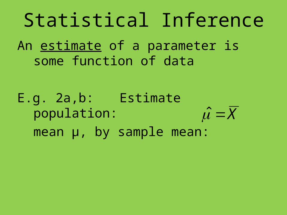
An estimate of a parameter is some function of data

Statistical InferenceA parameter is a numerical feature of
population, not sample
An estimate of a parameter is some function of data
(hopefully close to parameter)

Statistical InferenceAn estimate of a parameter is some function
of data
E.g. 1: Political Polls
Estimate population proportion, p, by
sample proportion: nXp ˆ

Statistical InferenceAn estimate of a parameter is some function
of data
E.g. 1: Political Polls
Estimate population proportion, p, by
sample proportion:
(same as before)
nXp ˆ
Statistical InferenceAn estimate of a parameter is some function
of data
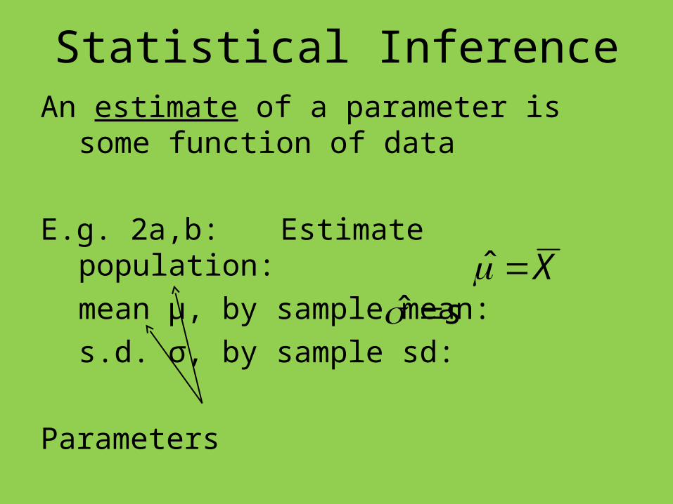
E.g. 2a,b: Estimate population:
mean μ, by sample mean: X

Statistical InferenceAn estimate of a parameter is some function
of data
E.g. 2a,b: Estimate population:
mean μ, by sample mean:
s.d. σ, by sample sd:
Xs
Statistical InferenceAn estimate of a parameter is some function
of data
E.g. 2a,b: Estimate population:
mean μ, by sample mean:
s.d. σ, by sample sd:
Parameters
Xs

Statistical InferenceAn estimate of a parameter is some function
of data
E.g. 2a,b: Estimate population:
mean μ, by sample mean:
s.d. σ, by sample sd:
Estimates
Xs

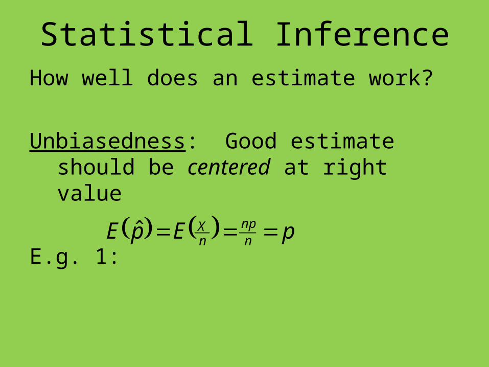
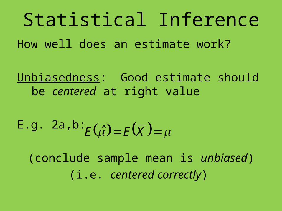
Statistical InferenceHow well does an estimate work?

Statistical InferenceHow well does an estimate work?
Unbiasedness: Good estimate should be centered at right value

Statistical InferenceHow well does an estimate work?
Unbiasedness: Good estimate should be centered at right value
(i.e. on average get right answer)

Statistical InferenceHow well does an estimate work?
Unbiasedness: Good estimate should be centered at right value
E.g. 1: pE ˆ

Statistical InferenceHow well does an estimate work?
Unbiasedness: Good estimate should be centered at right value
E.g. 1: nXEpE ˆ

Statistical InferenceHow well does an estimate work?
Unbiasedness: Good estimate should be centered at right value
E.g. 1: nnp
nXEpE ˆ
Statistical InferenceHow well does an estimate work?
Unbiasedness: Good estimate should be centered at right value
E.g. 1: pEpE nnp
nX ˆ

Statistical InferenceHow well does an estimate work?
Unbiasedness: Good estimate should be centered at right value
E.g. 1:
(conclude sample proportion is unbiased)
pEpE nnp
nX ˆ

Statistical InferenceHow well does an estimate work?
Unbiasedness: Good estimate should be centered at right value
E.g. 1:
(conclude sample proportion is unbiased)
(i.e. centered correctly)
pEpE nnp
nX ˆ

Statistical InferenceHow well does an estimate work?
Unbiasedness: Good estimate should be centered at right value
E.g. 2a,b: E

Statistical InferenceHow well does an estimate work?
Unbiasedness: Good estimate should be centered at right value
E.g. 2a,b: XEE

Statistical InferenceHow well does an estimate work?
Unbiasedness: Good estimate should be centered at right value
E.g. 2a,b: XEE ˆ
Statistical InferenceHow well does an estimate work?
Unbiasedness: Good estimate should be centered at right value
E.g. 2a,b:
(conclude sample mean is unbiased)
(i.e. centered correctly)
XEE ˆ

Statistical InferenceHow well does an estimate work?
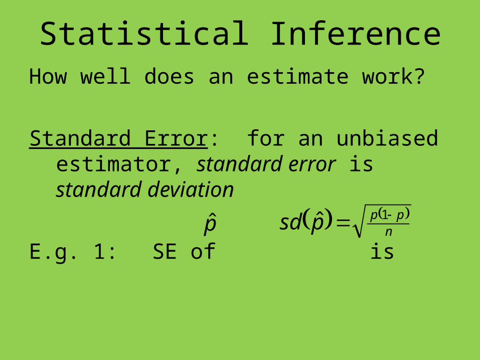
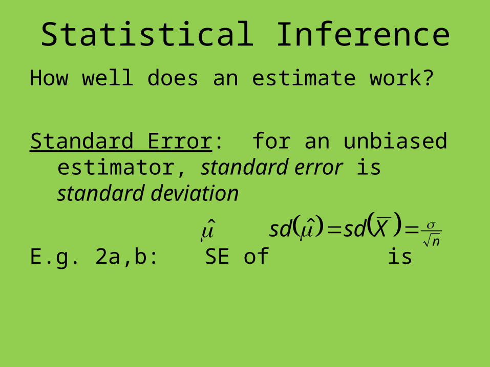
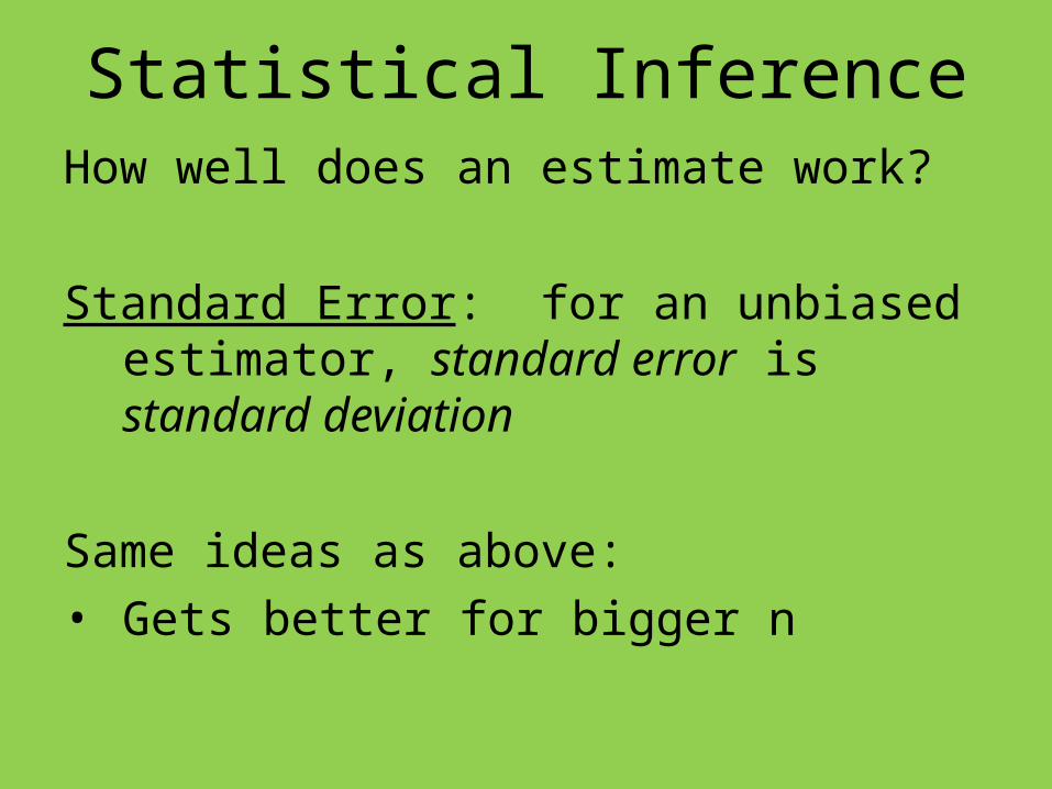
Standard Error: for an unbiased estimator, standard error is standard deviation
Statistical InferenceHow well does an estimate work?
Standard Error: for an unbiased estimator, standard error is standard deviation
E.g. 1: SE of is npppsd 1ˆp
Statistical InferenceHow well does an estimate work?
Standard Error: for an unbiased estimator, standard error is standard deviation
E.g. 2a,b: SE of is n
Xsdsd ˆ

Statistical InferenceHow well does an estimate work?
Standard Error: for an unbiased estimator, standard error is standard deviation
Same ideas as above
Statistical InferenceHow well does an estimate work?
Standard Error: for an unbiased estimator, standard error is standard deviation
Same ideas as above:
• Gets better for bigger n

Statistical InferenceHow well does an estimate work?
Standard Error: for an unbiased estimator, standard error is standard deviation
Same ideas as above:
• Gets better for bigger n
• By factor of n

Statistical InferenceHow well does an estimate work?
Standard Error: for an unbiased estimator, standard error is standard deviation
Same ideas as above:
• Gets better for bigger n
• By factor of
• Only new terminology
n

Statistical InferenceNice graphic on bias and variability:
Figure 3.14
From text

Statistical InferenceHW:
C22: Estimate the standard error of:
a. The estimate of the population proportion, p, when the sample proportion is 0.9, based on a sample of size 100. (0.03)
b. The estimate of the population mean, μ, when the sample standard deviation is s=15, based on a sample of size 25 (3)