Last Revised on January 8, 2015 Grade: EXPERIMENT 1physlabs/manuals/Experimen… · · 2015-01-08EXPERIMENT 1 Statistical Errors & Error ... Quite possibly the most used statistical

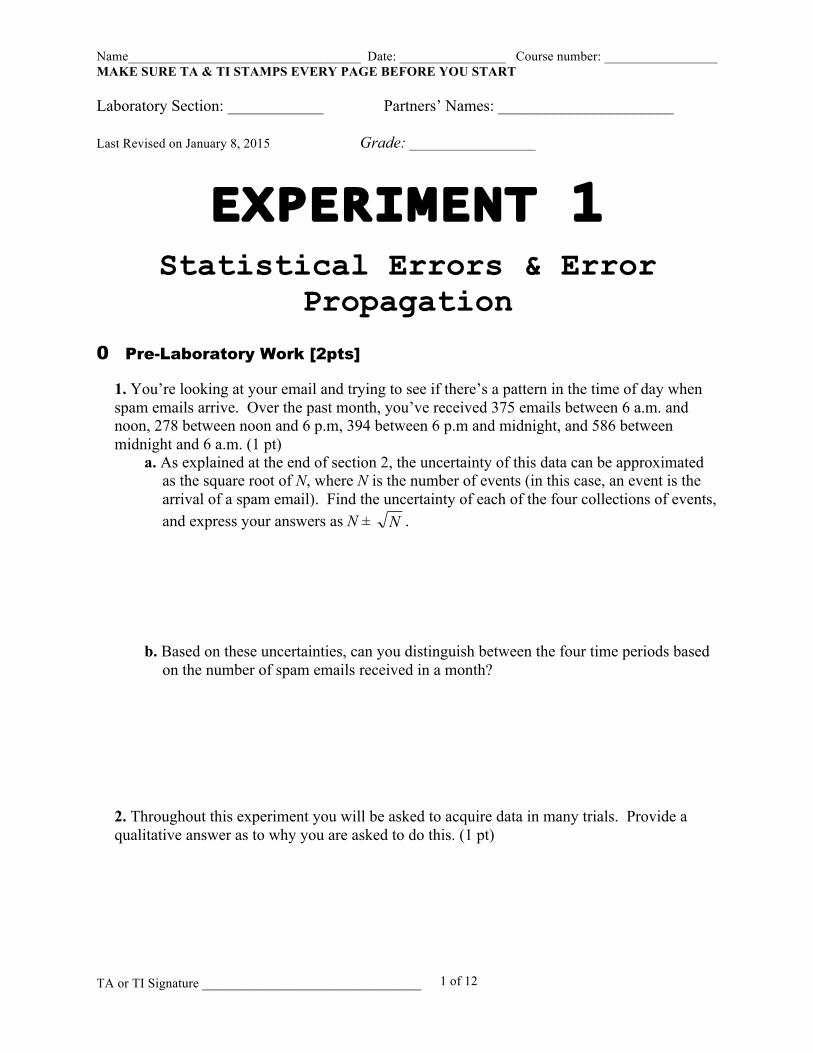
Name___________________________________ Date: ________________ Course number: _________________ MAKE SURE TA & TI STAMPS EVERY PAGE BEFORE YOU START

TA or TI Signature _________________________________

1 of 12

Laboratory Section: ____________ Partners’ Names: ______________________ Last Revised on January 8, 2015 Grade: ___________________

EXPERIMENT 1

Statistical Errors & Error Propagation

0 Pre-Laboratory Work [2pts]

1. You’re looking at your email and trying to see if there’s a pattern in the time of day when spam emails arrive. Over the past month, you’ve received 375 emails between 6 a.m. and noon, 278 between noon and 6 p.m, 394 between 6 p.m and midnight, and 586 between midnight and 6 a.m. (1 pt)

a. As explained at the end of section 2, the uncertainty of this data can be approximated as the square root of N, where N is the number of events (in this case, an event is the arrival of a spam email). Find the uncertainty of each of the four collections of events, and express your answers as N ± N .

b. Based on these uncertainties, can you distinguish between the four time periods based on the number of spam emails received in a month?

2. Throughout this experiment you will be asked to acquire data in many trials. Provide a qualitative answer as to why you are asked to do this. (1 pt)



2 of 12

EXPERIMENT 1

Statistical Errors & Error Propagation

1. Purpose

The purpose of this experiment is to understand statistical distributions and error propagation that can occur in their calculations. In addition, students will become familiar with the use and capabilities of a standard scientific calculator, as well as a digital Geiger counter. 2. Introduction Probability Distributions

Probability distributions are widely used in experiments that involve counting. Sampling errors that occur in counting experiments are called statistical errors. Statistical errors are one kind of error in a class of errors known as random errors. You will find that what you learn in this laboratory is relevant not only in the natural and social sciences, but also in everyday life.

You are probably familiar with polls conducted before a presidential election. If the sample of people who are polled was carefully chosen to represent the general population, then the error in the prediction would depend on the number of people in the sample. The larger the number of people in the sample, the smaller the error will be. If the sample were not properly chosen, it would result in a bias (i.e. a systematic error). Propagation of Error

In any calculation that occurs in science, there is always some inherent uncertainty as to the accuracy of the original measurement. Often times, this uncertainty stems from limitations in the measurement apparatus of the experiment (e.g. a ruler reading to only 1/10 of a centimeter). This uncertainty in measurement will propagate throughout the remaining calculations of that problem and will affect any further calculations and results, as we shall see in this experiment.

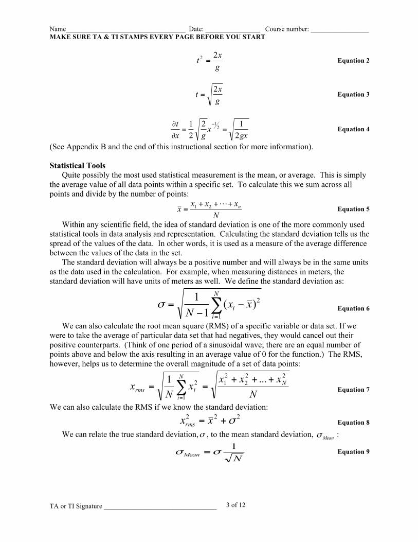
In an experiment involving simple motion, we can see that if an object is dropped it will follow Newton’s equations of motion (a free falling object) and should be defined by the equation:

2

21 gtx = Equation 1

where g is the gravitational constant and 28039.9 smg = on the earth’s surface. To solve for

xt∂∂

we must first isolate t on one side of the equation and then take the partial derivative with respect to x.



3 of 12

gxt 22 = Equation 2

gxt 2

= Equation 3

gx

xgx

t212

21 2

1==

∂

∂ − Equation 4

(See Appendix B and the end of this instructional section for more information).

Statistical Tools Quite possibly the most used statistical measurement is the mean, or average. This is simply the average value of all data points within a specific set. To calculate this we sum across all points and divide by the number of points:

N

xxxx n+++=

21 Equation 5

Within any scientific field, the idea of standard deviation is one of the more commonly used statistical tools in data analysis and representation. Calculating the standard deviation tells us the spread of the values of the data. In other words, it is used as a measure of the average difference between the values of the data in the set.

The standard deviation will always be a positive number and will always be in the same units as the data used in the calculation. For example, when measuring distances in meters, the standard deviation will have units of meters as well. We define the standard deviation as:

∑=

−−

=N

ii xx

N 1

2)(1

1σ Equation 6

We can also calculate the root mean square (RMS) of a specific variable or data set. If we were to take the average of particular data set that had negatives, they would cancel out their positive counterparts. (Think of one period of a sinusoidal wave; there are an equal number of points above and below the axis resulting in an average value of 0 for the function.) The RMS, however, helps us to determine the overall magnitude of a set of data points:

Nxxx

xN

x NN

iirms

222

21

1

2 ...1 +++== ∑

= Equation 7

We can also calculate the RMS if we know the standard deviation:

222 σ+= xxrms Equation 8

We can relate the true standard deviation,σ , to the mean standard deviation, Meanσ :

NMean1

σσ = Equation 9



4 of 12

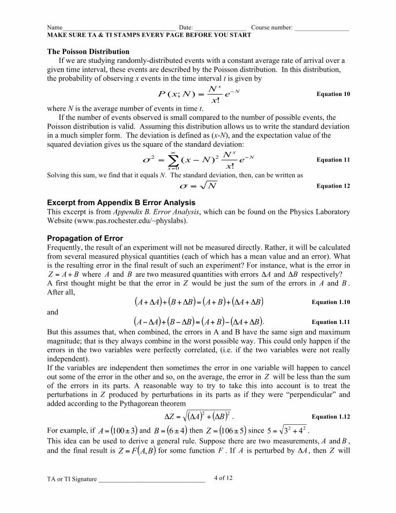
The Poisson Distribution If we are studying randomly-distributed events with a constant average rate of arrival over a given time interval, these events are described by the Poisson distribution. In this distribution, the probability of observing x events in the time interval t is given by

Nx

exNNxP −=!

);( Equation 10

where N is the average number of events in time t. If the number of events observed is small compared to the number of possible events, the Poisson distribution is valid. Assuming this distribution allows us to write the standard deviation in a much simpler form. The deviation is defined as (x-N), and the expectation value of the squared deviation gives us the square of the standard deviation:

∑∞

=

−−=0

22

!)(

x

Nx

exNNxσ Equation 11

Solving this sum, we find that it equals N. The standard deviation, then, can be written as N=σ Equation 12 Excerpt from Appendix B Error Analysis This excerpt is from Appendix B. Error Analysis, which can be found on the Physics Laboratory Website (www.pas.rochester.edu/~physlabs). Propagation of Error Frequently, the result of an experiment will not be measured directly. Rather, it will be calculated from several measured physical quantities (each of which has a mean value and an error). What is the resulting error in the final result of such an experiment? For instance, what is the error in

BAZ += where A and B are two measured quantities with errors AΔ and BΔ respectively? A first thought might be that the error in Z would be just the sum of the errors in A and B . After all, ( ) ( ) ( ) ( )BABABBAA Δ+Δ++=Δ++Δ+ Equation 1.10 and ( ) ( ) ( ) ( )BABABBAA Δ+Δ−+=Δ−+Δ− . Equation 1.11 But this assumes that, when combined, the errors in A and B have the same sign and maximum magnitude; that is they always combine in the worst possible way. This could only happen if the errors in the two variables were perfectly correlated, (i.e. if the two variables were not really independent). If the variables are independent then sometimes the error in one variable will happen to cancel out some of the error in the other and so, on the average, the error in Z will be less than the sum of the errors in its parts. A reasonable way to try to take this into account is to treat the perturbations in Z produced by perturbations in its parts as if they were “perpendicular” and added according to the Pythagorean theorem ( ) ( )22 BAZ Δ+Δ=Δ . Equation 1.12

For example, if ( )3100±=A and ( )46±=B then ( )5106±=Z since 22 435 += . This idea can be used to derive a general rule. Suppose there are two measurements, A andB , and the final result is ( )BAFZ ,= for some function F . If A is perturbed by AΔ , then Z will



5 of 12

be perturbed by AAF

Δ⎟⎠

⎞⎜⎝

⎛∂∂ , where (the partial derivative)

AF∂∂ is the derivative of F with respect

to A with B held constant. Similarly, the perturbation in Z due to a perturbation in B is

BBF

Δ⎟⎠

⎞⎜⎝

⎛∂∂ . Combining these by the Pythagorean Theorem yields

( ) ( )22

22

BBFA

AFZ Δ⎟

⎠

⎞⎜⎝

⎛∂∂

+Δ⎟⎠

⎞⎜⎝

⎛∂∂

=Δ . Equation 1.13

In the example of BAZ += considered above,

1=∂∂AF and 1=

∂∂BF ,

so this gives the same result as before. Similarly, if BAZ −= , then

1=∂∂AF and 1−=

∂∂BF ,

which also gives the same result. However, if ABZ = , then,

BAF=

∂∂ and A

BF=

∂∂ ,

so ( ) ( )2222 BAABZ Δ+Δ=Δ . Equation 1.14

Thus,

22

⎟⎠

⎞⎜⎝

⎛ Δ+⎟⎠

⎞⎜⎝

⎛ Δ=Δ

=Δ

BB

AA

ABZ

ZZ Equation 1.15

or the fractional error in Z is the square root of the sum of the squares of the fractional errors in its parts. It should be noted that since the above applies only when the two measured quantities are independent of each other, it does not apply when, for example, one physical quantity is measured and what is required is its square. If 2AZ = , then the perturbation in Z due to a perturbation in A is

AAAAFZ Δ=Δ∂∂

= 2 . Equation 1.16

Thus, in this case,

( ) ⎟⎠

⎞⎜⎝

⎛ Δ±=Δ±=Δ+

AAAAAAAA 212 222 Equation 1.17

and not ⎟⎠

⎞⎜⎝

⎛ Δ±

AAA 212 as would be obtained by misapplying the rule for independent variables.

For example, ( ) 20100110 2 ±=± and not 14100± . If a variable Z depends on one or two variables A or/and B , which have independent errors AΔ and BΔ , then the rules for calculating the error in Z is tabulated in Table 1.4 for a variety

of simple relationships. These rules may be compounded for more complicated situations.



6 of 12

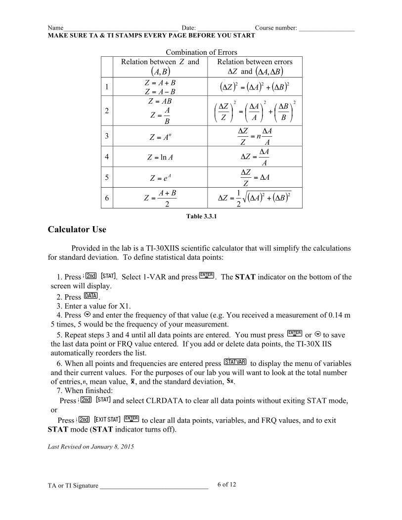
Combination of Errors

Relation between Z and

( )BA, Relation between errors

ZΔ and ( )BA ΔΔ ,

1 BAZ += BAZ −= ( ) ( ) ( )222 BAZ Δ+Δ=Δ

2 ABZ =

BAZ =

222

⎟⎠

⎞⎜⎝

⎛ Δ+⎟⎠

⎞⎜⎝

⎛ Δ=⎟⎠

⎞⎜⎝

⎛ ΔBB

AA

ZZ

3 nAZ = AAn

ZZ Δ=

Δ

4 AZ ln= AAZ Δ

=Δ

5 AeZ = AZZ

Δ=Δ

6 2BAZ +

= ( ) ( )22

21 BAZ Δ+Δ=Δ

Table 3.3.1

Calculator Use Provided in the lab is a TI-30XIIS scientific calculator that will simplify the calculations for standard deviation. To define statistical data points:

1. Press . Select 1-VAR and press . The STAT indicator on the bottom of the screen will display.

2. Press . 3. Enter a value for X1. 4. Press and enter the frequency of that value (e.g. You received a measurement of 0.14 m

5 times, 5 would be the frequency of your measurement. 5. Repeat steps 3 and 4 until all data points are entered. You must press or to save

the last data point or FRQ value entered. If you add or delete data points, the TI-30X IIS automatically reorders the list.

6. When all points and frequencies are entered press to display the menu of variables and their current values. For the purposes of our lab you will want to look at the total number of entries, , mean value, , and the standard deviation, .

7. When finished: Press and select CLRDATA to clear all data points without exiting STAT mode, or

Press to clear all data points, variables, and FRQ values, and to exit STAT mode (STAT indicator turns off). Last Revised on January 8, 2015



7 of 12

EXPERIMENT 1 Statistical Errors & Error

Propagation 3. Gravitational Acceleration of Ruler

3.1 Introduction This experiment consists of dropping a ruler and determining which lab partner has the faster

reaction time based upon the distance that he or she allows the ruler to pass before they catch the ruler with their hands.

The following items are to be given to each student: • One (1) ½ meter stick

3.2 Procedure

1. One lab partner will hold the ½ meter stick at the end of the meter stick (the 50 cm end)

and hold it up as high as they are comfortably able to.

2. The second lab partner will be catching the ½ meter stick as it falls. To set up for this, place your thumb and pointer finger about 1 ½ inches apart and place your hand at the 0 cm mark of the ½ meter stick, so that the tops of your fingers are roughly equal with the zero mark on the ½ meter stick.

3. Without warning, the lab partner holding the ½ meter stick should release it and the other lab partner should react as quickly as possible and catch it as quickly as they are able by closing their fingers and not moving their arms.

4. Note the distance that the ruler has traveled according to the tops of your fingers and round up to the nearest whole centimeter. Record your result in Table 3.3.1. Repeat this procedure 24 more times, for a total of 25 trials.

5. Lab partners should switch roles and repeat steps 1-4 so that there are two data sets, each with 25 trials.



8 of 12

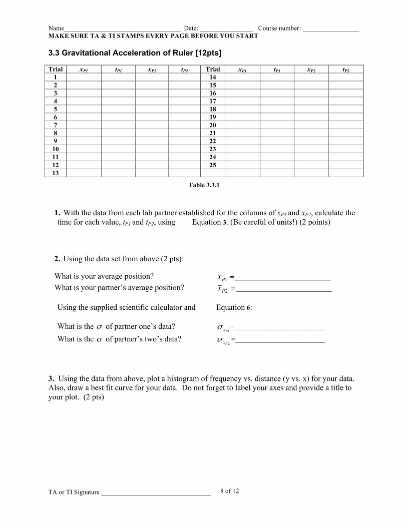
3.3 Gravitational Acceleration of Ruler [12pts] Trial xP1 tP1 xP2 tP2 Trial xP1 tP1 xP2 tP2

1 14 2 15 3 16 4 17 5 18 6 19 7 20 8 21 9 22

10 23 11 24 12 25 13

Table 3.3.1

1. With the data from each lab partner established for the columns of xP1 and xP2, calculate the time for each value, tP1 and tP2, using Equation 3. (Be careful of units!) (2 points)

2. Using the data set from above (2 pts): What is your average position? =1Px ________________________

What is your partner’s average position? =2Px ________________________ Using the supplied scientific calculator and Equation 6: What is the σ of partner one’s data?

1Pxσ =___________________________

What is the σ of partner’s two’s data? 2Px

σ =___________________________

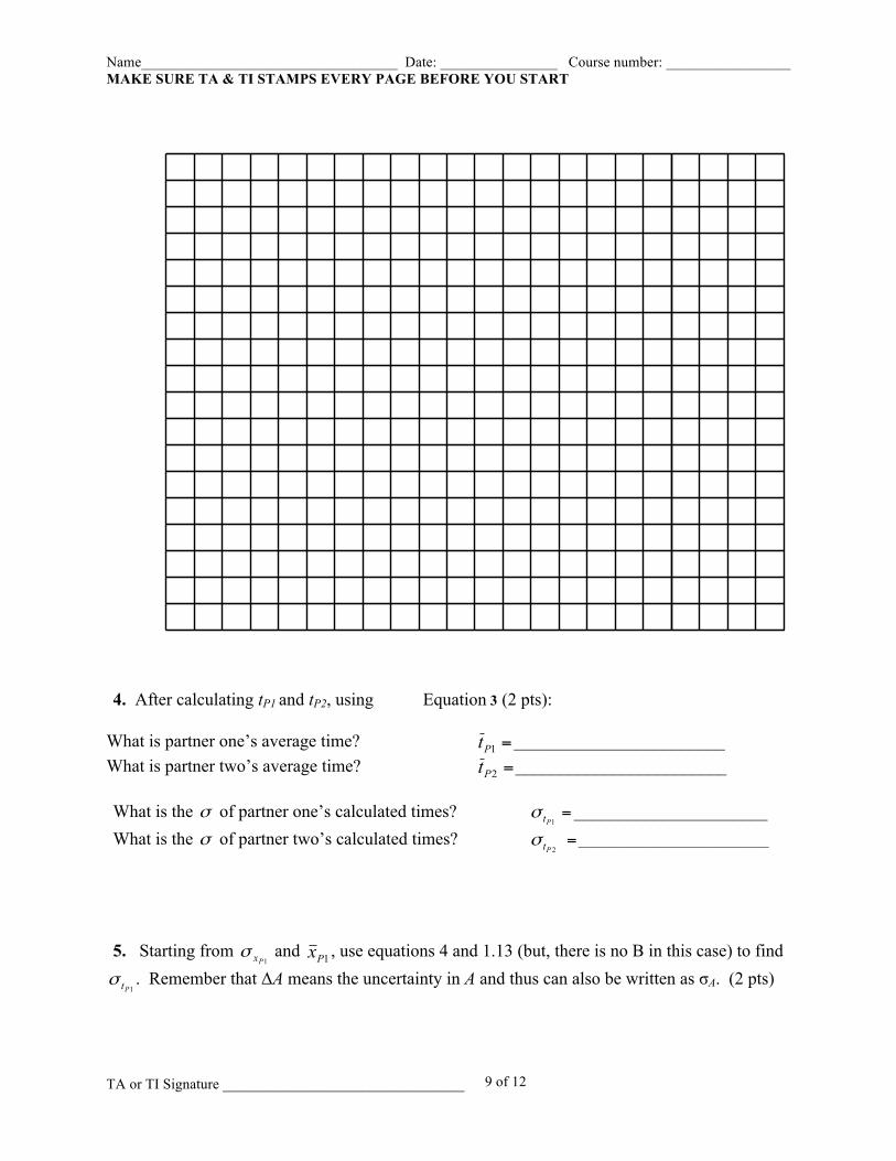
3. Using the data from above, plot a histogram of frequency vs. distance (y vs. x) for your data. Also, draw a best fit curve for your data. Do not forget to label your axes and provide a title to your plot. (2 pts)



9 of 12

4. After calculating tP1 and tP2, using Equation 3 (2 pts): What is partner one’s average time? =1Pt ________________________

What is partner two’s average time? =2Pt ________________________ What is the σ of partner one’s calculated times? =

1Ptσ ______________________

What is the σ of partner two’s calculated times? =2Pt

σ __________________________

5. Starting from

1Pxσ and 1Px , use equations 4 and 1.13 (but, there is no B in this case) to find

1Ptσ . Remember that ΔA means the uncertainty in A and thus can also be written as σA. (2 pts)



10 of 12

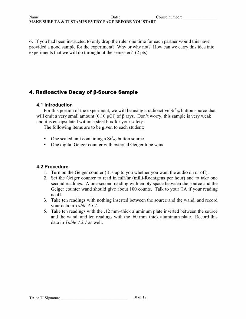
6. If you had been instructed to only drop the ruler one time for each partner would this have provided a good sample for the experiment? Why or why not? How can we carry this idea into experiments that we will do throughout the semester? (2 pts) 4. Radioactive Decay of β-Source Sample

4.1 Introduction For this portion of the experiment, we will be using a radioactive Sr+

90 button source that will emit a very small amount (0.10 µCi) of β rays. Don’t worry, this sample is very weak and it is encapsulated within a steel box for your safety.

The following items are to be given to each student:

• One sealed unit containing a Sr+90 button source

• One digital Geiger counter with external Geiger tube wand

4.2 Procedure 1. Turn on the Geiger counter (it is up to you whether you want the audio on or off). 2. Set the Geiger counter to read in mR/hr (milli-Roentgens per hour) and to take one

second readings. A one-second reading with empty space between the source and the Geiger counter wand should give about 100 counts. Talk to your TA if your reading is off.

3. Take ten readings with nothing inserted between the source and the wand, and record your data in Table 4.3.1.

5. Take ten readings with the .12 mm–thick aluminum plate inserted between the source and the wand, and ten readings with the .60 mm–thick aluminum plate. Record this data in Table 4.3.1 as well.



11 of 12

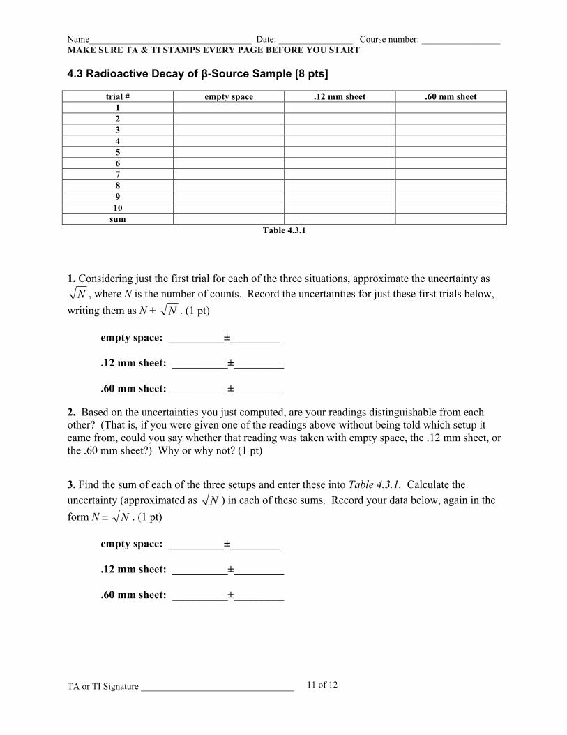
4.3 Radioactive Decay of β-Source Sample [8 pts]

trial # empty space .12 mm sheet .60 mm sheet 1 2 3 4 5 6 7 8 9

10 sum

Table 4.3.1 1. Considering just the first trial for each of the three situations, approximate the uncertainty as N , where N is the number of counts. Record the uncertainties for just these first trials below,

writing them as N ± N . (1 pt) empty space: __________±_________ .12 mm sheet: __________±_________ .60 mm sheet: __________±_________ 2. Based on the uncertainties you just computed, are your readings distinguishable from each other? (That is, if you were given one of the readings above without being told which setup it came from, could you say whether that reading was taken with empty space, the .12 mm sheet, or the .60 mm sheet?) Why or why not? (1 pt) 3. Find the sum of each of the three setups and enter these into Table 4.3.1. Calculate the uncertainty (approximated as N ) in each of these sums. Record your data below, again in the form N ± N . (1 pt) empty space: __________±_________ .12 mm sheet: __________±_________ .60 mm sheet: __________±_________



12 of 12

4. Based on the uncertainties you computed, are these sums distinguishable from each other? Why or why not? Compare your answer with your answer to question 2 and explain any differences. (1 pt) 5. For the empty space data, how many trials are within one standard deviation of the average? How many are within two standard deviations? (1 pt) 6. Sketch a picture of what the inside of the black box looks like – where is the radioactive source? Where is the Geiger counter wand? Where does the aluminum sheet that you insert go? (Think about why inserting this sheet causes the reading of mR/hr to decrease.) (1 pt) 7. Imagine you had taken 100 readings rather than 10 for each of the setups. As an estimate of what you would observe, multiply each of the sums from Question 3 by 10. Now re-calculate the uncertainty for each of the setups using these new sums. Are the readings distinguishable from each other? How do these uncertainties compare with the uncertainties based on 10 readings? (1pt) 8. If you were designing an experiment to distinguish between empty space and the .12-mm sheet, how many trials would you run? Be as quantitative as possible. (1 pt)

Documents

Last Revised on January 8, 2015 Grade: EXPERIMENT 1physlabs/manuals/Experimen… · · 2015-01-08EXPERIMENT 1 Statistical Errors & Error ... Quite possibly the most used statistical