Laser Doppler Flowometry

A.K.Khachatryan. Final Report, Phys 173, UCSD Laboratory of Optics and Biophysics. Performed under the supervision of Dr. Phlbert Tsai Doppler Effect analysis has proven to be a useful forensic tool for a variety of studies in physical and biological sciences. Having been used in fields varying such as astronomy, acoustics, vibrational analysis and flow research, it is now a major contributor to the advancement of research in biophysics and biomedical sciences. The objective of this paper is to provide a report of a technique known as Laser Doppler Flowometry (LDF) which uses relativistic doppler shift analysis to determine the velocity of particles suspended in a moving fluid. A direct application of LDF in medicine is in the field of hemodynamics research that seeks to quantify the flow of blood in human tissue. LDF is a highly favorable technique as it is noninvasive and is performed without causing a disturbance in the surrounding patterns of fluid flow or the tissue. Introduction and Background Theory Relativistic Doppler Effect is a phenomenon related to electromagnetic waves, in this case - light. It is the change in frequency, and therefore the wavelength of light caused by relative motion of the incident light beam and the moving particle. As the two beams come in to contact with the particle at their focal point, they become scattered and pick up the particle’s velocity component, therefore acquiring a change in their frequency. The relativistic doppler shift (RDS) formula reads

                                                                                                   F!"##$%&   = 2 !"#(!/!)!!"

V! *

where F!"##$%&   is the difference between the frequencies of the two scattered beams, θ is the angle between the incident beams, λ  is the wavelength of the incident beams and V!  is the velocity of the particle.

Fig. 1. Beam scattering at contact with moving particle

fsb1 = fib1 + fib1(vpuib )c

= fib1(1+vpuib1λib

)

fsb2 = fib2 + fib2(vpuib )c

= fib2 (1+vpuib1λib

)

fdoppler = fsb2 − fsb1

fdoppler = 2sin(θ / 2)

λibvp

Two laser beams are focused at a point where the scattering particle is in motion. Fig. 1 shows IB1 ad IB2 (the 1st and 2nd incident beams respectively) coming to a focal point where the particle is in motion with velocity vector vp . Vectors

uib1 and uib2 are unit

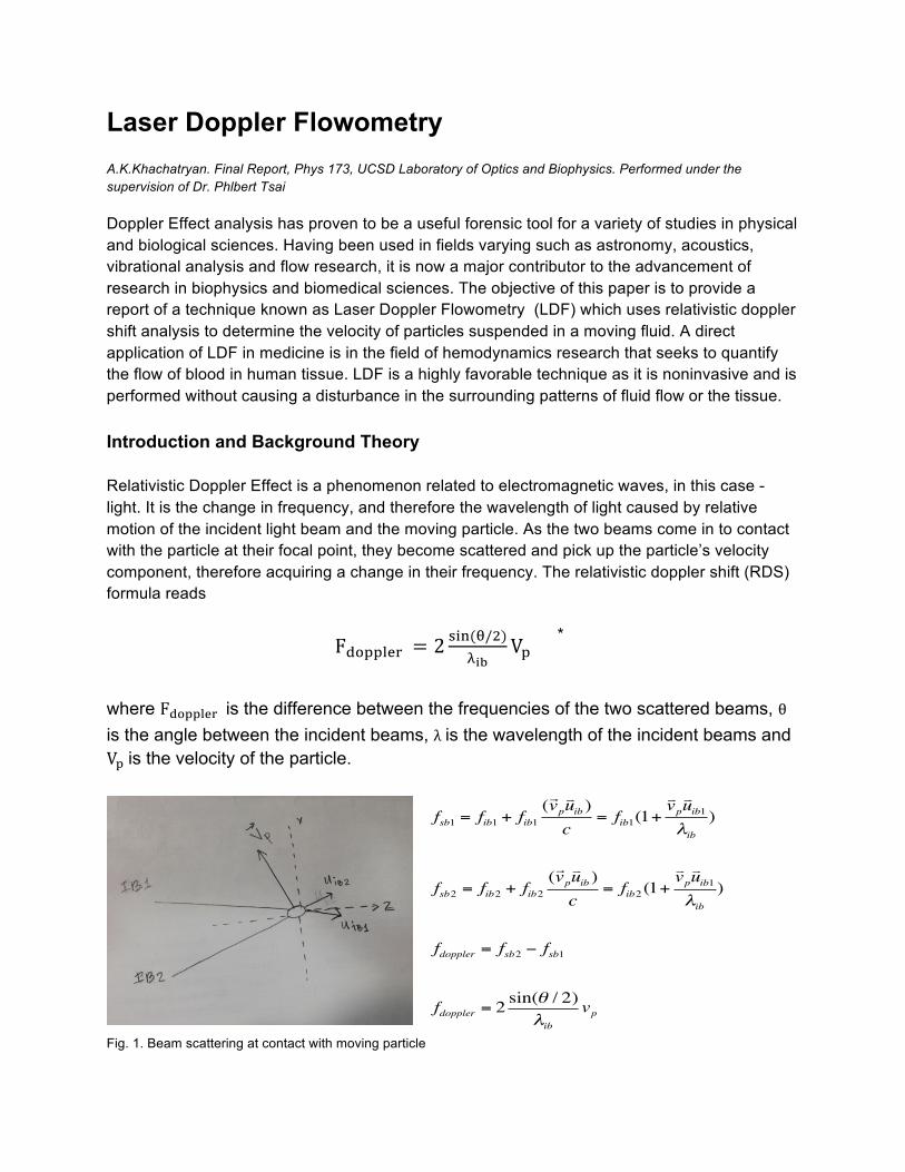
vectors in the direction of the IB1 and IB2 respectively. Methods Experimental Set-up To produce the desired scattering effects for the RDS to work, an experimental set-up was designed as shown in Fig. 2.

Fig. 2. Experimental Setup: Two-Beam Configuration for LDF A helium-neon laser of power 8mW was used which produced a red beam of light of 635nm wavelength. The beam was sent through a prism that split the beam into two beams (Beam 1 and Beam 2 in Fig. 2) perpendicular to one another. A mirror was used to collimate the two beams. The parallel beams were then sent through an objective lens that focused them at the center of the tube containing the moving fluid with particles in it. A couple of other lenses were then used to collect, collimate and lastly to focus the scattered beams onto a photodetector. Flow Tube A gravity pump was made to allow for fluid to pass through the tube at constant velocity. The tube used was of 0.2x2.0 mm in dimensions and was much smaller in size compared to the reservoir of 50ml volume. The relatively large size of the reservoir is desired so that the change in pressure throughout the reservoir is negligible relative to the flow tube in the small amount of time period within which the data was recorded. This allows for the assumed constancy of the velocity of fluid in the flow tube.

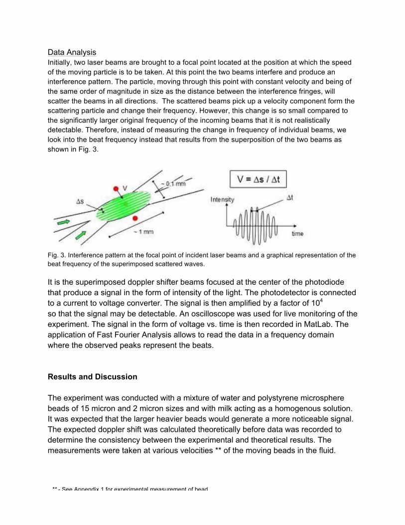
Data Analysis Initially, two laser beams are brought to a focal point located at the position at which the speed of the moving particle is to be taken. At this point the two beams interfere and produce an interference pattern. The particle, moving through this point with constant velocity and being of the same order of magnitude in size as the distance between the interference fringes, will scatter the beams in all directions. The scattered beams pick up a velocity component form the scattering particle and change their frequency. However, this change is so small compared to the significantly larger original frequency of the incoming beams that it is not realistically detectable. Therefore, instead of measuring the change in frequency of individual beams, we look into the beat frequency instead that results from the superposition of the two beams as shown in Fig. 3.

Fig. 3. Interference pattern at the focal point of incident laser beams and a graphical representation of the beat frequency of the superimposed scattered waves. It is the superimposed doppler shifter beams focused at the center of the photodiode that produce a signal in the form of intensity of the light. The photodetector is connected to a current to voltage converter. The signal is then amplified by a factor of 104

so that the signal may be detectable. An oscilloscope was used for live monitoring of the experiment. The signal in the form of voltage vs. time is then recorded in MatLab. The application of Fast Fourier Analysis allows to read the data in a frequency domain where the observed peaks represent the beats. Results and Discussion The experiment was conducted with a mixture of water and polystyrene microsphere beads of 15 micron and 2 micron sizes and with milk acting as a homogenous solution. It was expected that the larger heavier beads would generate a more noticeable signal. The expected doppler shift was calculated theoretically before data was recorded to determine the consistency between the experimental and theoretical results. The measurements were taken at various velocities ** of the moving beads in the fluid.

** - See Appendix 1 for experimental measurement of bead

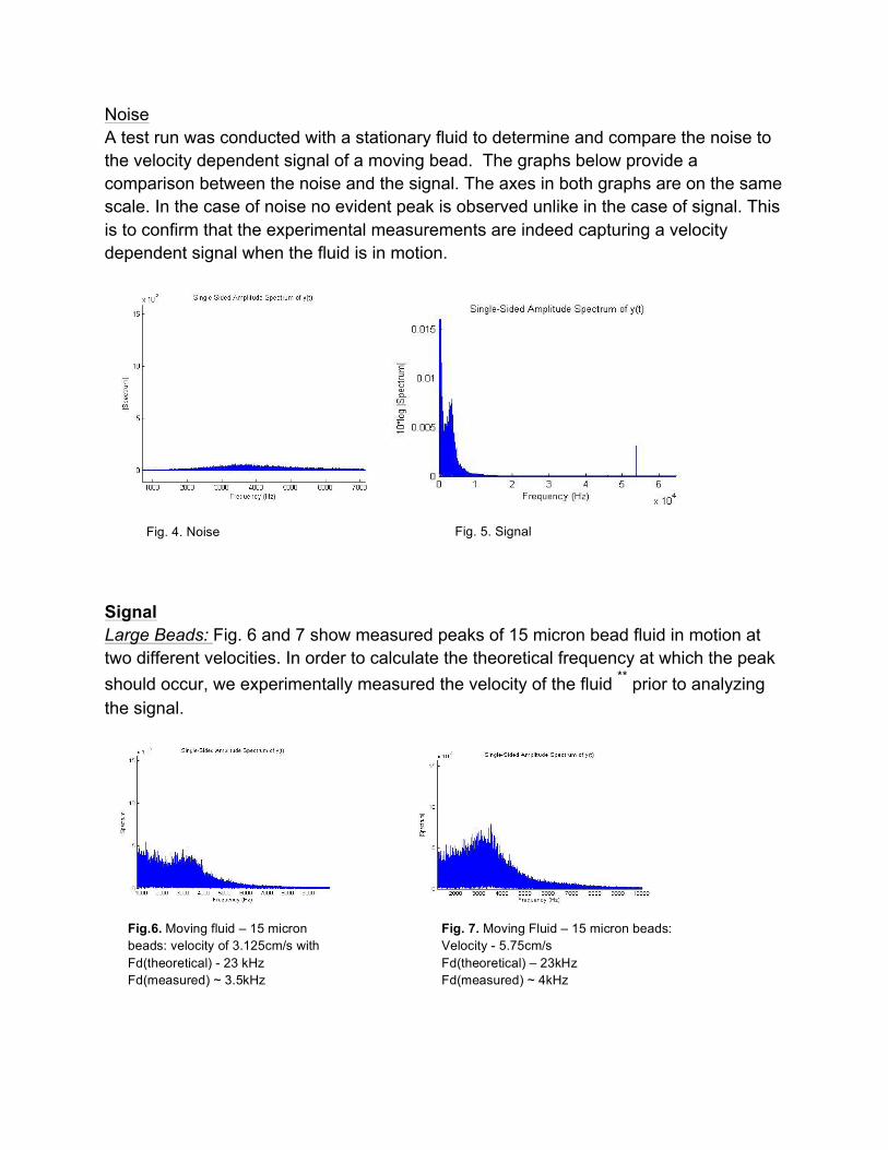
Noise A test run was conducted with a stationary fluid to determine and compare the noise to the velocity dependent signal of a moving bead. The graphs below provide a comparison between the noise and the signal. The axes in both graphs are on the same scale. In the case of noise no evident peak is observed unlike in the case of signal. This is to confirm that the experimental measurements are indeed capturing a velocity dependent signal when the fluid is in motion.

Signal Large Beads: Fig. 6 and 7 show measured peaks of 15 micron bead fluid in motion at two different velocities. In order to calculate the theoretical frequency at which the peak should occur, we experimentally measured the velocity of the fluid ** prior to analyzing the signal.

Fig. 4. Noise Fig. 5. Signal

Fig.6. Moving fluid – 15 micron beads: velocity of 3.125cm/s with Fd(theoretical) - 23 kHz Fd(measured) ~ 3.5kHz

Fig. 7. Moving Fluid – 15 micron beads: Velocity - 5.75cm/s Fd(theoretical) – 23kHz Fd(measured) ~ 4kHz

The results showed a velocity dependent signal: the signal for a bead moving at larger velocity produced a higher peak compared to a slower moving bead therefore confirming the assumption that the power of the doppler shifted frequency spectrum is directly proportional to the velocity of the scattering particle. We also see a small shift in the peak towards a higher frequency for the particle with larger velocity also validating the presence of the detected beats. However, there is an inconsistency between experimental and theoretical frequency at which the peak should appear. In both cases at the given velocities of the particle, the peak was observed at a much smaller frequency than expected.

Factors contributing to inconsistent results might be due to inaccurate experimental velocity measurements.

First, the 15 micron beads are large and heavy enough in size to interfere with the assumed experimental variables. The gravitational effects are higher on larger sized beads. This can prevent the beads being uniformly mixed in the water and moving at the same speed. Also assuming laminar flow, our experimental measurements of velocity of the fluid could have been an inaccurate representation of the actual velocity of the beads because the large heavy beads are expected to move slower than the water around them. Particles moving at various speeds in a non-uniformly mixed fluid will scatter beams with different intensities causing a wider range of frequency spectrum for the peaks. To correct for this error smaller sized beads should be used.

Second, Boundary conditions were not taken into consideration. A flow of a fluid in a tube is non-uniform in velocity throughout the tube. Closer to the walls of the tube the fluid will move slower than the fluid at the center of the tube. It is of utmost importance to make sure the focus of the beams is placed at the center of the tube to get a better estimate of the overall velocity of the fluid. This can also be improved by using a larger tube to better differentiate between the center and the boundaries of the tube. Small beads and uniform homogeneous mixture: Same methods as described for the 15 micron beads were used to collect data for the 2 micron beads as well as for heavily diluted milk. Milk was used as an analogue to a homogeneous solution under the assumption that all particles in it should move at roughly the same speed. The results for the 2 micron beads very closely resembled the results for milk, therefore, we only include data for milk sample.

A small peak was detected compared to much larger amounts of noise for the sample. This makes it more difficult to interpret the results. The most probable cause for this may be due to the size of the beads or the particles in the milk being small enough for Brownian motion to become relevant. The slower peak in the noise for the stationary fluid is near the predicted velocity for the Brownian motion ***. This makes it difficult to distinguish between the true velocity of the particles moving in the fluid and the velocity of the particles due thermal fluctuations. Therefore, the experiment can be improved to produce better interpretable data if the size of the particles is large enough so that the effects of Brownian motion are negligible.

*** - See Appendix 2 for calculations of Brownian velocity of beads

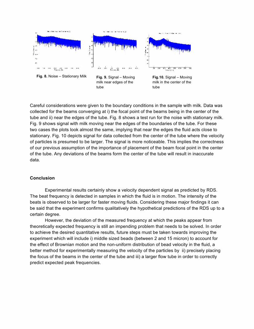
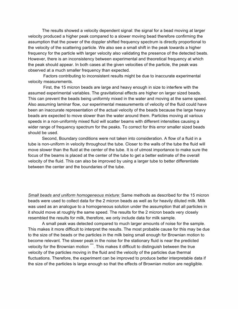
Careful considerations were given to the boundary conditions in the sample with milk. Data was collected for the beams converging at i) the focal point of the beams being in the center of the tube and ii) near the edges of the tube. Fig. 8 shows a test run for the noise with stationary milk. Fig. 9 shows signal with milk moving near the edges of the boundaries of the tube. For these two cases the plots look almost the same, implying that near the edges the fluid acts close to stationary. Fig. 10 depicts signal for data collected from the center of the tube where the velocity of particles is presumed to be larger. The signal is more noticeable. This implies the correctness of our previous assumption of the importance of placement of the beam focal point in the center of the tube. Any deviations of the beams form the center of the tube will result in inaccurate data. Conclusion

Experimental results certainly show a velocity dependent signal as predicted by RDS. The beat frequency is detected in samples in which the fluid is in motion. The intensity of the beats is observed to be larger for faster moving fluids. Considering these major findings it can be said that the experiment confirms qualitatively the hypothetical predictions of the RDS up to a certain degree.

However, the deviation of the measured frequency at which the peaks appear from theoretically expected frequency is still an impending problem that needs to be solved. In order to achieve the desired quantitative results, future steps must be taken towards improving the experiment which will include i) middle sized beads (between 2 and 15 micron) to account for the effect of Brownian motion and the non-uniform distribution of bead velocity in the fluid, a better method for experimentally measuring the velocity of the particles by ii) precisely placing the focus of the beams in the center of the tube and iii) a larger flow tube in order to correctly predict expected peak frequencies.

Fig. 8. Noise – Stationary Milk Fig. 9. Signal – Moving milk near edges of the tube

Fig.10. Signal – Moving milk in the center of the tube

Appendix 1

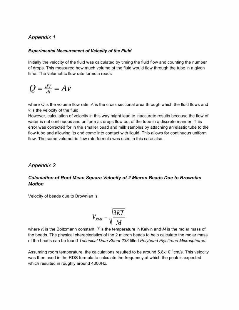
Experimental Measurement of Velocity of the Fluid Initially the velocity of the fluid was calculated by timing the fluid flow and counting the number of drops. This measured how much volume of the fluid would flow through the tube in a given time. The volumetric flow rate formula reads

Q = dVdt = Av

where Q is the volume flow rate, A is the cross sectional area through which the fluid flows and v is the velocity of the fluid. However, calculation of velocity in this way might lead to inaccurate results because the flow of water is not continuous and uniform as drops flow out of the tube in a discrete manner. This error was corrected for in the smaller bead and milk samples by attaching an elastic tube to the flow tube and allowing its end come into contact with liquid. This allows for continuous uniform flow. The same volumetric flow rate formula was used in this case also. Appendix 2 Calculation of Root Mean Square Velocity of 2 Micron Beads Due to Brownian Motion Velocity of beads due to Brownian is

where K is the Boltzmann constant, T is the temperature in Kelvin and M is the molar mass of the beads. The physical characteristics of the 2 micron beads to help calculate the molar mass of the beads can be found Technical Data Sheet 238 titled Polybead Plystirene Microspheres. Assuming room temperature, the calculations resulted to be around 5.8x10-1 cm/s. This velocity was then used in the RDS formula to calculate the frequency at which the peak is expected which resulted in roughly around 4000Hz.

VRMS =3KTM

References

Kalkert, C., and J. Kayser. Laser Doppler Flowometry. Rep. UCSD/David Kleinfeld Laboratory.

Web. 10 Apr. 2014.

Keenan, L., and K. Chapin. Laser Doppler Velocimetry. Rep. UCSD/David Kleinfeld

Laboratory. Web. 10 Apr. 2014.

"Polybead Polystyrene Microspheres." Polysciences, Inc Chemistry Beyond the Ordinary. Web.

May-June 2014.

<http://www.polysciences.com/SiteData/docs/TDS238/d060e1ed6379b508/TDS%202

38.pdf>.

Tornos, J., M. A. Robelledo, and J. M. Alvarez. Laser Doppler Velocimetry Experiment with a

Water Flow to Measure the Fourier Transform of the Time -Interval Probability;

Comparison Between Experimental and Theoretical Results. APS/Physical Review,

June-July 1989. Web. 2 May 2014.