Large-Scale FPGA-based Convolutional Networks

Clement Farabet1, Yann LeCun1, Koray Kavukcuoglu1,Eugenio Culurciello2, Berin Martini2,

Polina Akselrod2, Selcuk Talay2

1. The Courant Institute of Mathematical Sciences, New York University, New York, USA

2: Electrical Engineering Department, Yale University, New Haven, USA

Chapter in Machine Learning on Very Large Data Sets,edited by Ron Bekkerman, Mikhail Bilenko, and John Langford,

Cambridge University Press, 2011.

May 2, 2011

1

Large-Scale FPGA-Based Convolutional NetworksMicro-robots, unmanned aerial vehicles (UAVs), imaging sensor networks,

wireless phones, and other embedded vision systems all require low cost andhigh-speed implementations of synthetic vision systems capable of recognizingand categorizing objects in a scene.

Many successful object recognition systems use dense features extracted onregularly-spaced patches over the input image. The majority of the feature ex-traction systems have a common structure composed of a filter bank (generallybased on oriented edge detectors or 2D gabor functions), a non-linear operation(quantization, winner-take-all, sparsification, normalization, and/or point-wisesaturation) and finally a pooling operation (max, average or histogramming).For example, the scale-invariant feature transform (SIFT (Lowe, 2004)) operatorapplies oriented edge filters to a small patch and determines the dominant orien-tation through a winner-take-all operation. Finally, the resulting sparse vectorsare added (pooled) over a larger patch to form local orientation histogram.Some recognition systems use a single stage of feature extractors (Lazebniket al., 2006; Dalal and Triggs, 2005; Berg et al., 2005; Pinto et al., 2008).

Other models like HMAX-type models (Serre et al., 2005; Mutch and Lowe,2006) and convolutional networks use two more layers of successive feature ex-tractors. Different training algorithms have been used for learning the parame-ters of convolutional networks. In LeCun et al. (1998b) and Huang and LeCun(2006), pure supervised learning is used to update the parameters. However, re-cent works have focused on training with an auxiliary task (Ahmed et al., 2008)or using unsupervised objectives (Ranzato et al., 2007b; Kavukcuoglu et al.,2009; Jarrett et al., 2009; Lee et al., 2009).

This chapter presents a scalable hardware architecture for large-scale multi-layered synthetic vision systems based on large parallel filter banks, such as con-volutional networks. This hardware can also be used to accelerate the execution(and partial learning) of recent vision algorithms like SIFT and HMAX (Lazeb-nik et al., 2006; Serre et al., 2005). This system is a data-flow vision enginethat can perform real-time detection, recognition and localization in mega-pixelimages processed as pipelined streams. The system was designed with the goalof providing categorization of an arbitrary number of objects, while consumingvery little power.

Graphics Processing Units (GPUs) are becoming a common alternative tocustom hardware in vision applications, as demonstrated in (Coates et al., 2009).Their advantage over custom hardware are numerous: they are inexpensive,available in most recent computers, and easily programmable with standarddevelopment kits, such as nVidia CUDA SDK. The main reasons for continuingdeveloping custom hardware are twofold: performance and power consumption.By developing a custom architecture that is fully adapted to a certain rangeof tasks (as is shown in this chapter), the product of power consumption byperformance can be improved by a factor of 100.

1 Learning Internal Representations

One of the key questions of Vision Science (natural and artificial) is how toproduce good internal representations of the visual world. What sort of internal

2

representation would allow an artificial vision system to detect and classifyobjects into categories, independently of pose, scale, illumination, conformation,and clutter? More interestingly, how could an artificial vision system learnappropriate internal representations automatically, the way animals and humansseem to learn by simply looking at the world? In the time-honored approach tocomputer vision (and to pattern recognition in general), the question is avoided:internal representations are produced by a hand-crafted feature extractor, whoseoutput is fed to a trainable classifier. While the issue of learning features hasbeen a topic of interest for many years, considerable progress has been achievedin the last few years with the development of so-called deep learning methods.

Good internal representations are hierarchical. In vision, pixels are assem-bled into edglets, edglets into motifs, motifs into parts, parts into objects, andobjects into scenes. This suggests that recognition architectures for vision (andfor other modalities such as audio and natural language) should have multipletrainable stages stacked on top of each other, one for each level in the featurehierarchy. This raises two new questions: what to put in each stage? and how totrain such deep, multi-stage architectures? Convolutional Networks (ConvNets)are an answer to the first question. Until recently, the answer to the secondquestion was to use gradient-based supervised learning, but recent research indeep learning has produced a number of unsupervised methods which greatlyreduce the need for labeled samples.

1.1 Convolutional Networks

convolutional network!overview

Input dataFeature

Pooling: P

Linear

Classifier

Feature

Extraction: F+N+RF+N+R

{ } at (xi,yi)

Object

Categories

{ } at (xj,yj)

{ } at (xk,yk)

R_abs: RectificationF: Filter Bank N: Normalization

Figure 1: Architecture of a typical convolutional network for object recognition.This implements a convolutional feature extractor and a linear classifier forgeneric N-class object recognition. Once trained, the network can be computedon arbitrary large input images, producing a classification map as output.

Convolutional Networks (LeCun et al., 1990, 1998b) are trainable architec-

3

tures composed of multiple stages. The input and output of each stage are setsof arrays called feature maps. For example, if the input is a color image, eachfeature map would be a 2D array containing a color channel of the input image(for an audio input each feature map would be a 1D array, and for a video orvolumetric image, it would be a 3D array). At the output, each feature maprepresents a particular feature extracted at all locations on the input. Eachstage is composed of three layers: a filter bank layer, a non-linearity layer, anda feature pooling layer. A typical ConvNet is composed of one, two or threesuch 3-layer stages, followed by a classification module.

Each layer type is now described for the case of image recognition. We intro-duce the following convention: banks of images will be seen as three dimensionalarrays in which the first dimension is the number of independent maps/images,the second is the height of the maps and the third is the width. The input bankof a module is denoted x, the output bank y, an image in the input bank xi, apixel in the input bank xijk.

• Filter Bank Layer - F : the input is a 3D array with n1 2D feature mapsof size n2 × n3. Each component is denoted xijk, and each feature mapis denoted xi. The output is also a 3D array, y composed of m1 featuremaps of size m2 ×m3. A trainable filter (kernel) kij in the filter bank hassize l1 × l2 and connects input feature map xi to output feature map yj .The module computes

yj = bj +∑

i

kij ∗ xi (1)

where bj is a trainable bias parameter, and ∗ is the 2D discrete convolutionoperator:

(kij ∗ xi)pq =

l1/2−1∑

m=−l1/2

l2/2−1∑

n=−l2/2

kij,m,nxi,p+m,q+n. (2)

Each filter detects a particular feature at every location on the input.Hence spatially translating the input of a feature detection layer will trans-late the output but leave it otherwise unchanged.

• Non-Linearity Layer - R,N : In traditional ConvNets this simply con-sists in a pointwise tanh function applied to each site (ijk). However,recent implementations have used more sophisticated non-linearities. Auseful one for natural image recognition is the rectified tanh: Rabs(x) =abs(gi.tanh(x)) where gi is a trainable gain parameter per each input fea-ture map i. The rectified tanh is sometimes followed by a subtractive anddivisive local normalization N , which enforces local competition betweenadjacent features in a feature map, and between features at the closebyspatial locations. Local competition usually results in features that aredecorrelated, thereby maximizing their individual role. The subtractivenormalization operation for a given site xijk computes:

4

vijk = xijk −∑

ipq

wpq.xi,j+p,k+q, (3)

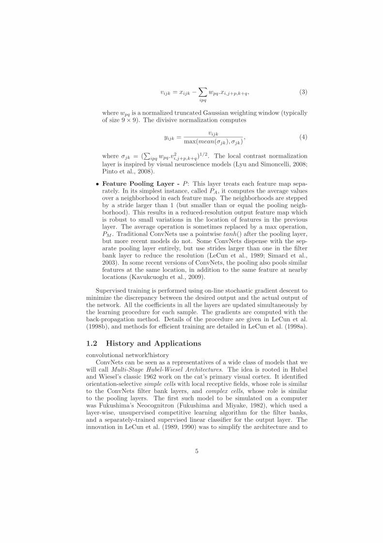
where wpq is a normalized truncated Gaussian weighting window (typicallyof size 9× 9). The divisive normalization computes

yijk =vijk

max(mean(σjk), σjk), (4)

where σjk = (∑

ipq wpq.v2i,j+p,k+q)

1/2. The local contrast normalization

layer is inspired by visual neuroscience models (Lyu and Simoncelli, 2008;Pinto et al., 2008).

• Feature Pooling Layer - P : This layer treats each feature map sepa-rately. In its simplest instance, called PA, it computes the average valuesover a neighborhood in each feature map. The neighborhoods are steppedby a stride larger than 1 (but smaller than or equal the pooling neigh-borhood). This results in a reduced-resolution output feature map whichis robust to small variations in the location of features in the previouslayer. The average operation is sometimes replaced by a max operation,PM . Traditional ConvNets use a pointwise tanh() after the pooling layer,but more recent models do not. Some ConvNets dispense with the sep-arate pooling layer entirely, but use strides larger than one in the filterbank layer to reduce the resolution (LeCun et al., 1989; Simard et al.,2003). In some recent versions of ConvNets, the pooling also pools similarfeatures at the same location, in addition to the same feature at nearbylocations (Kavukcuoglu et al., 2009).

Supervised training is performed using on-line stochastic gradient descent tominimize the discrepancy between the desired output and the actual output ofthe network. All the coefficients in all the layers are updated simultaneously bythe learning procedure for each sample. The gradients are computed with theback-propagation method. Details of the procedure are given in LeCun et al.(1998b), and methods for efficient training are detailed in LeCun et al. (1998a).

1.2 History and Applications

convolutional network!historyConvNets can be seen as a representatives of a wide class of models that we

will call Multi-Stage Hubel-Wiesel Architectures. The idea is rooted in Hubeland Wiesel’s classic 1962 work on the cat’s primary visual cortex. It identifiedorientation-selective simple cells with local receptive fields, whose role is similarto the ConvNets filter bank layers, and complex cells, whose role is similarto the pooling layers. The first such model to be simulated on a computerwas Fukushima’s Neocognitron (Fukushima and Miyake, 1982), which used alayer-wise, unsupervised competitive learning algorithm for the filter banks,and a separately-trained supervised linear classifier for the output layer. Theinnovation in LeCun et al. (1989, 1990) was to simplify the architecture and to

5

use the back-propagation algorithm to train the entire system in a supervisedfashion.

The approach was very successful, and led to several implementations, rang-ing from optical character recognition (OCR) to object detection, scene segmen-tation, and robot navigation:

• check reading (handwriting recognition) at AT&T (LeCun et al., 1998b)and Microsoft (Simard et al., 2003; Chellapilla et al., 2006),

• detection in images, including faces with record accuracy and real-timeperformance (Vaillant et al., 1994; Garcia and Delakis, 2004; Osadchyet al., 2007; Nasse et al., 2009), license plates and faces in Google’s StreetView (Fromeet al., 2009), or customers’ gender and age at NEC,

• more experimental detection of hands/gestures (Nowlan and Platt, 1995),logos and text (Delakis and Garcia, 2008),

• vision-based navigation for off-road robots: in the DARPA-sponsoredLAGR program, ConvNets were used for long-range obstacle detection (Had-sell et al., 2009). In Hadsell et al. (2009), the system is pre-trained off-lineusing a combination of unsupervised learning (as described in section 1.3)and supervised learning. It is then adapted on-line, as the robot runs,using labels provided by a short-range stereovision system (see videos athttp://www.cs.nyu.edu/~yann/research/lagr),

• interesting new applications include image restoration (Jain and Seung,2008) and image segmentation, particularly for biological images (Ninget al., 2005).

Over the years, other instances of the Multi-Stage Hubel-Wiesel Architec-ture have appeared that are in the tradition of the Neocognitron: unlike su-pervised ConvNets, they use a combination of hand-crafting, and simple unsu-pervised methods to design the filter banks. Notable examples include Mozer’svisual models (Mozer, 1991), and the so-called HMAX family of models fromT. Poggio’s lab at MIT (Serre et al., 2005; Mutch and Lowe, 2006), which useshard-wired Gabor filters in the first stage, and a simple unsupervised randomtemplate selection algorithm for the second stage. All stages use point-wisenon-linearities and max pooling. From the same institute, Pinto et al. (Pintoet al., 2008) have identified the most appropriate non-linearities and normaliza-tions by running systematic experiments with a single-stage architecture usingGPU-based parallel hardware.

1.3 Unsupervised Learning of ConvNets

convolutional network!unsupervised learningTraining deep, multi-stage architectures using supervised gradient back prop-

agation requires many labeled samples. However in many problems labeled datais scarce whereas unlabeled data is abundant. Recent research in deep learn-ing (Hinton and Salakhutdinov, 2006; Bengio et al., 2007; Ranzato et al., 2007a)has shown that unsupervised learning can be used to train each stage one af-ter the other using only unlabeled data, reducing the requirement for labeled

6

samples significantly. In Jarrett et al. (2009), using abs and normalizationnon-linearities, unsupervised pre-training, and supervised global refinement hasbeen shown to yield excellent performance on the Caltech-101 dataset with only30 training samples per category (more on this below). In Lee et al. (2009),good accuracy was obtained on the same set using a very different unsupervisedmethod based on sparse Restricted Boltzmann Machines. Several works at NEChave also shown that using auxiliary tasks (Ahmed et al., 2008; Weston et al.,2008) helps regularizing the system and produces excellent performance.

1.3.1 Unsupervised Training with Predictive Sparse Decomposition

The unsupervised method we propose, to learn the filter coefficients in the filterbank layers, is called Predictive Sparse Decomposition (PSD) (Kavukcuogluet al., 2008). Similar to the well-known sparse coding algorithms (Olshausenand Field, 1997), inputs are approximated as a sparse linear combination ofdictionary elements.

Z∗ = minZ

‖X −WZ‖22 + λ|Z|1 (5)

In conventional sparse coding ( 5), for any given input X, an expensive op-timization algorithm is run to find the optimal sparse representation Z∗ (the“basis pursuit” problem). PSD trains a non-linear feed-forward regressor (orencoder) C(X,K) = g.(tanh(X ∗ k+ b)) to approximate the sparse solution Z∗.During training, the feature vector Z∗ is obtained by minimizing the followingcompound energy:

E(Z,W,K) = ‖X −WZ‖22 + λ‖Z‖1 + ‖Z − C(X,K)‖22 (6)

where W is the matrix whose columns are the dictionary elements and K =k, g, b are the encoder filter, bias and gain parameters. For each training sampleX, one first finds Z∗ that minimizes E, then W and K are adjusted by one stepof stochastic gradient descent to lower E. Once training is complete, the featurevector for a given input is simply approximated with Z∗ = C(X,K), hence theprocess is extremely fast (feed-forward).

1.3.2 Results on Object Recognition

convolutional network!object recognitionIn this section, various architectures and training procedures are compared

to determine which non-linearities are preferable, and which training protocolmakes a difference.

Generic Object Recognition using Caltech 101 Dataset. Caltech 101is a standard dataset of labeled images, containing 101 categories of objects inthe wild.

We use a two-stage system where, the first stage is composed of an F layerwith 64 filters of size 9× 9, followed by different combinations of non-linearitiesand pooling. The second-stage feature extractor is fed with the output of thefirst stage and extracts 256 output features maps, each of which combines a

7

Table 1: Average recognition rates on Caltech-101 with 30 training samplesper class. Each row contains results for one of the training protocols (U =unsupervised, X = random, + = supervised fine-tuning), and each column forone type of architecture (F = filter bank, PA = average pooling, PM = maxpooling, R = rectification, N = normalization).

Single Stage [64.F9×9 −R/N/P5×5 − logreg]F−Rabs −N−PA F−Rabs −PA F−N−PM F−PA

U+ 54.2% 50.0% 44.3% 14.5%X+ 54.8% 47.0% 38.0% 14.3%U 52.2% 43.3% 44.0% 13.4%X 53.3% 31.7% 32.1% 12.1%

Two Stages [256.F9×9 −R/N/P4×4 − logreg]F−Rabs −N−PA F−Rabs −PA F−N−PM F−PA

U+ 65.5% 60.5% 61.0% 32.0%X+ 64.7% 59.5% 60.0% 29.7%U 63.7% 46.7% 56.0% 9.1%X 62.9% 33.7% 37.6% 8.8%

random subset of 16 feature maps from the previous stage using 9 × 9 kernels.Hence the total number of convolution kernels is 256× 16 = 4096.

Table 1 summarizes the results for the experiments, where U and X denotesunsupervised pre-training and random initialization respectively, and + denotessupervised fine-tuning of the whole system.1. Excellent accuracy of 65.5% is obtained using unsupervised pre-training andsupervised refinement with abs and normalization non-linearities. The resultis on par with the popular model based on SIFT and pyramid match kernelSVM (Lazebnik et al., 2006). It is clear that abs and normalization are crucialfor achieving good performance. This is an extremely important fact for usersof convolutional networks, which traditionally only use tanh().2. Astonishingly, random filters without any filter learning whatsoever achievedecent performance (62.9% for X), as long as abs and normalization are present(Rabs − N − PA). A more detailed study on this particular case can be foundin Jarrett et al. (2009).3. Comparing experiments from rows X vs X+, U vs U+, we see that super-vised fine tuning consistently improves the performance, particularly with weaknon-linearities.4. It seems that unsupervised pre-training (U , U+) is crucial when newly pro-posed non-linearities are not in place.

Handwritten Digit Classification using MNIST Dataset. MNIST is adataset of handwritten digits (LeCun and Cortes, 1998): it contains 60, 000 28×28 image patches of digits on uniform backgrounds, and a standard testing set of10, 000 different samples, widely used by the vision community as a benchmarkfor algorithms. Each patch is labeled with a number ranging from 0 to 9.

Using the evidence gathered in previous experiments, we used a two-stagesystem with a two-layer fully-connected classifier to learn the mapping between

8

the samples’ pixels and the labels. The two convolutional stages were pre-trained unsupervised (without the labels), and refined supervised (with the la-bels). An error rate of 0.53% was achieved on the test set. To our knowledge,this is the lowest error rate ever reported on the original MNIST dataset, with-out distortions or preprocessing. The best previously reported error rate was0.60% (Ranzato et al., 2007a).

1.3.3 Connection with Other Approaches in Object Recognition

Many recent successful object recognition systems can also be seen as singleor multi-layer feature extraction systems followed by a classifier. Most commonfeature extraction systems like SIFT (Lowe, 2004), HoG (Dalal and Triggs, 2005)are composed of filter banks (oriented edge detectors at multiple scales) followedby non-linearities (winner take all) and pooling (histogramming). A PyramidMatch Kernel (PMK) SVM (Lazebnik et al., 2006) classifier can also be seen asanother layer of feature extraction since it performs a K-means based featureextraction followed by local histogramming.

2 A Dedicated Digital Hardware Architecture

convolutional network!hardware architecture FPGA ASICBiologically inspired vision models, and more generally image processing al-

gorithms are usually expressed as sequences of operations or transformations.They can be well described by a modular approach, in which each module pro-cesses an input image bank and produces a new bank. Figure 1 is a graphicalillustration of this approach. Each module requires the previous bank to be fully(or at least partially) available before computing its output. This causality pre-vents simple parallelism to be implemented across modules. However parallelismcan easily be introduced within a module, and at several levels, depending onthe kind of underlying operations.

In the following discussion, banks of images will be seen as three dimensionalarrays in which the first dimension is the number of independent maps/images,the second is the height of the maps and the third is the width. As in section 1.1,the input bank of a module is denoted x, the output bank y, an image in theinput bank xi, a pixel in the input bank xijk. Input banks’ dimensions will benoted n1×n2×n3, output banks m1×m2×m3. Each module implements a typeof operation that requires K operations per input pixel xijk. The starting pointof the discussion is a general purpose processor composed of an arithmetic unit, afast internal cache of size SINT , and an external memory of size SEXT >> SINT .The bandwidth between the internal logic and the external memory array willbe noted BEXT .

The coarsest level of parallelism can be obtained at the image bank level. Amodule that applies a unary transformation to produce one output image foreach input image (n1 = m1) can be broken up in n1 independent threads. Thisis the most basic form of parallelism, and it finds its limits when n2×n3 becomeslarger than a threshold, closely related to SINT . In fact, past a certain size, thenumber of pixels that can be processed in a given time equals BEXT /(2 ×K)

9

(bandwidth is shared between writes and reads). In other terms, the amount ofparallelism that can be introduced at this level is limited by BEXT /K.

A finer level of parallelism can be introduced at the operation level. The costof fetching pixels from the external memory being very high, the most efficientform of parallelism can occur when pixels are reused in multiple operations(K > 1). It can be shown that optimal performances are reached ifK operationscan be produced in parallel in the arithmetic unit. In other terms, the amountof parallelism that can be introduced at this level is limited by BEXT .

If the internal cache size SINT is large enough to hold all the images of theentire set of modules to compute, then the overall performance of the system ifdefined by BINT , the bandwidth between the arithmetic unit and the internalcache. The size of internal memory caches growing according to Moore’s Law,more data can fit internally, which naturally pulls performances of computationsfrom K ×BEXT to K ×BINT .

For a given technology though, SINT has an upper bound, and the onlypart of the system we can act upon is the internal architecture. Based onthese observations, our approach is to tackle the problem of producing the Kparallel operations by rethinking the architecture of the arithmetic units, whileconserving the traditional external memory storage. Our problem can be statedsimply:

Problem 1. K being the number of operations performed per input pixel;BEXT being the bandwidth available between the arithmetic units and theexternal memory array; we want to establish an architecture that produces Koperations in parallel, so that BEXT is fully utilized.

2.1 A Data-Flow Approach

data-flow computingThe data-flow hardware architecture was initiated by Adams (1969), and

quickly became an active field of research (Dennis and Misunas, 1974; Hickset al., 1993; l. Gaudiot et al., 1994). Cho et al. (2008) presents one of the latestdata-flow architectures that has several similarities to the approach presentedhere.

Figure 2 shows a data-flow architecture whose goal is to process homogeneousstreams of data in parallel (Farabet et al., 2010). It is defined around severalkey ideas:

• a 2D grid of NPT Processing Tiles (PTs) that contain:

– a bank of processing operators. An operator can be anything from aFIFO to an arithmetic operator, or even a combination of arithmeticoperators. The operators are connected to local data lines,

– a routing multiplexer (MUX). The MUX connects the local data linesto global data lines or to neighboring tiles.

• a Smart Direct Memory Access module (Smart DMA), that interfacesoff-chip memory and provides asynchronous data transfers, with prioritymanagement,

10

11

X +

%

MUX.

X +

%

MUX.

X +

%

MUX.

X +

%

MUX.

X +

∑π %

MUX.

X +

%

MUX.

X +

%

MUX.

X +

%

MUX.

X +

%

MUX.

Control

& Config

Smart DMA

Configurable Route Global Data Lines Runtime Config Bus

Off-chip

Memory

Mem∑π Mem∑π Mem

∑π Mem ∑π Mem

∑π Mem∑π Mem

∑π Mem

∑π Mem

A Runtime Reconfigurable Dataflow Architecture

PT PT PT

PTPTPT

PT PT PT

Figure 2: A data-flow computer. A set of runtime configurable processing tilesare connected on a 2D grid. They can exchange data with their 4 neighbors andwith an off-chip memory via global lines.

• a set of Nglobal global data lines used to connect PTs to the Smart DMA,Nglobal << NPT ,

• a set of local data lines used to connect PTs with their 4 neighbors,

• a Runtime Configuration Bus, used to reconfigure many aspects of thegrid at runtime—connections, operators, Smart DMA modes. . . (the con-figurable elements are depicted as squares on Fig.2),

• a controller that can reconfigure most of the computing grid and the SmartDMA at runtime.

2.1.1 On Runtime Reconfiguration

reconfigurable hardwareOne of the most interesting aspects of this grid is its configuration capabil-

ities. Many systems have been proposed which are based on two-dimensionalarrays of processing elements interconnected by a routing fabric that is reconfig-urable. Field Programmable Gate Arrays (FPGAs) for instance, offer one of themost versatile grid of processing elements. Each of these processing elements—usually a simple look-up table—can be connected to any of the other elementsof the grid, which provides with the most generic routing fabric one can thinkof. Thanks to the simplicity of the processing elements, the number that canbe packed in a single package is in the order of 104 to 105. The drawback is thereconfiguration time, which takes in the order of milliseconds, and the synthesistime, which takes in the order of minutes to hours depending on the complexityof the circuit.

At the other end of the spectrum, recent multicore processors implementonly a few powerful processing elements (in the order of 10s to 100s). For thesearchitectures, no synthesis is involved, instead, extensions to existing program-ming languages are used to explicitly describe parallelism. The advantage ofthese architectures is the relative simplicity of use: the implementation of analgorithm rarely takes more than a few days, whereas months are required fora typical circuit synthesis for FPGAs.

The architecture presented here is at the middle of this spectrum. Buildinga fully generic data-flow computer is a tedious task. Reducing the spectrum ofapplications to the image processing problem—as stated in Problem 1—allowsus to define the following constraints:

• high throughput is a top priority, low latency is not. Indeed, most ofthe operations performed on images are replicated over both dimensionsof these images, usually bringing the amount of similar computations toa number that is much larger than the typical latencies of a pipelinedprocessing unit,

• therefore each operator has to provide with a maximum throughput (e.g.one operation per clock cycle) to the detriment of any initial latency, andhas to be stallable (e.g. must handle discontinuities in data streams).

• configuration time has to be low, or more precisely in the order of thesystem’s latency. This constraint simply states that the system should be

12

able to reconfigure itself between two kinds of operations in a time thatis negligible compared to the image sizes. That is a crucial point to allowruntime reconfiguration,

• the processing elements in the grid should be as coarse grained as per-mitted, to maximize the ratio between computing logic and routing logic.Creating a grid for a particular application (e.g. ConvNets) allows the useof very coarse operators. On the other hand, a general purpose grid hasto cover the space of standard numeric operators,

• the processing elements, although they might be complex, should not haveany internal state, but should just passively process any incoming data.The task of sequencing operations is done by a global control unit thatsimply configures the entire grid for a given operation, lets the data flowin, and prepares the following operation.

The first two points of this list are crucial to create a flexible data-flowsystem. Several types of grids have been proposed in the past (Dennis andMisunas, 1974; Hicks et al., 1993; Kung, 1986), often trying to solve the duallatency/throughput problem, and often providing a computing fabric that is toorigid.

The grid proposed here provides a flexible processing framework, due to thestallable nature of the operators. Indeed, any paths can be configured on thegrid, even paths that require more bandwidth that is actually feasible. Insteadof breaking, each operator will stall its pipeline when required. This is achievedby the use of FIFOs at the input and output of each operators, that compensatefor bubbles in the data streams, and force the operators to stall when they arefull. Any sequence of operators can then be easily created, without concern forbandwidth issues.

The third point is achieved by the use of a runtime configuration bus, com-mon to all units. Each module in the design has a set of configurable parameters,routes or settings (depicted as squares on Figure 2), and possesses a unique ad-dress on the network. Groups of similar modules also share a broadcast address,which dramatically speeds up reconfiguration of elements that need to performsimilar tasks.

The last point depicts the data-flow idea of having (at least theoretically)no state, or instruction pointer. In the case of the system presented here, thegrid has no state, but a state does exit in a centralized control unit. For eachconfiguration of the grid, no state is used, and the presence of data drivesthe computations. Although this leads to an optimal throughput, the systempresented here strives to be as general as possible, and having the possibility ofconfiguring the grid quickly to perform a new type of operation is crucial to runalgorithms that require different types of computations.

A typical execution of an operation on this system is the following: (1)the control unit configures each tile to be used for the computation and eachconnection between the tiles and their neighbors and/or the global lines, bysending a configuration command to each of them, (2) it configures the SmartDMA to prefetch the data to be processed, and to be ready to write resultsback to off-chip memory, (3) when the DMA is ready, it triggers the streamingout, (4) each tile processes its respective incoming streaming data, and passes

13

the results to another tile, or back to the Smart DMA, (5) the control unit isnotified of the end of operations when the Smart DMA has completed.

X +

∑π %

MUX.

Mem

PT

56

7

X +

%

MUX.

X +

∑π %

MUX.

X +

%

MUX.

X +

%

MUX.

Smart DMA.

Configurable Route Active Data Lines

Off-chip

Memory

Mem

∑π Mem∑π Mem∑π Mem

PT

PT PT PT

Active Route

1

23

4

X +

∑π %

MUX.

Mem

PT

89

X +

∑π %

MUX.

Mem

PT

56

7

X +

∑π %

MUX.

Mem

PT

23

4

X +

∑π %

MUX.

Mem

PT

89

1

10

1111

13 12

14

16 15

17

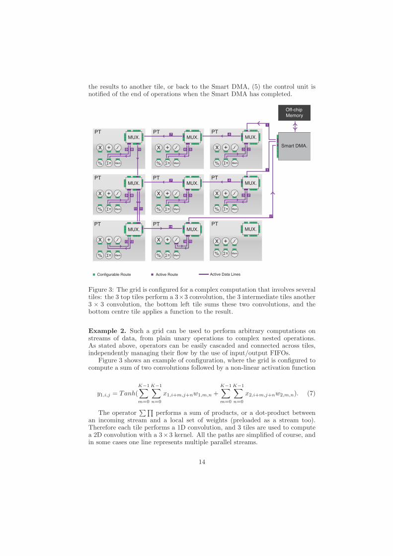
Figure 3: The grid is configured for a complex computation that involves severaltiles: the 3 top tiles perform a 3×3 convolution, the 3 intermediate tiles another3 × 3 convolution, the bottom left tile sums these two convolutions, and thebottom centre tile applies a function to the result.

Example 2. Such a grid can be used to perform arbitrary computations onstreams of data, from plain unary operations to complex nested operations.As stated above, operators can be easily cascaded and connected across tiles,independently managing their flow by the use of input/output FIFOs.

Figure 3 shows an example of configuration, where the grid is configured tocompute a sum of two convolutions followed by a non-linear activation function

y1,i,j = Tanh(

K−1∑

m=0

K−1∑

n=0

x1,i+m,j+nw1,m,n +

K−1∑

m=0

K−1∑

n=0

x2,i+m,j+nw2,m,n). (7)

The operator∑∏

performs a sum of products, or a dot-product betweenan incoming stream and a local set of weights (preloaded as a stream too).Therefore each tile performs a 1D convolution, and 3 tiles are used to computea 2D convolution with a 3×3 kernel. All the paths are simplified of course, andin some cases one line represents multiple parallel streams.

14

It can be noted that this last example provides a nice solution to Problem 1.Indeed, the input data being 2 images x1 and x2, and the output data oneimage y1, the K operations are performed in parallel, and the entire operationis achieved at a bandwidth of BEXT /3.

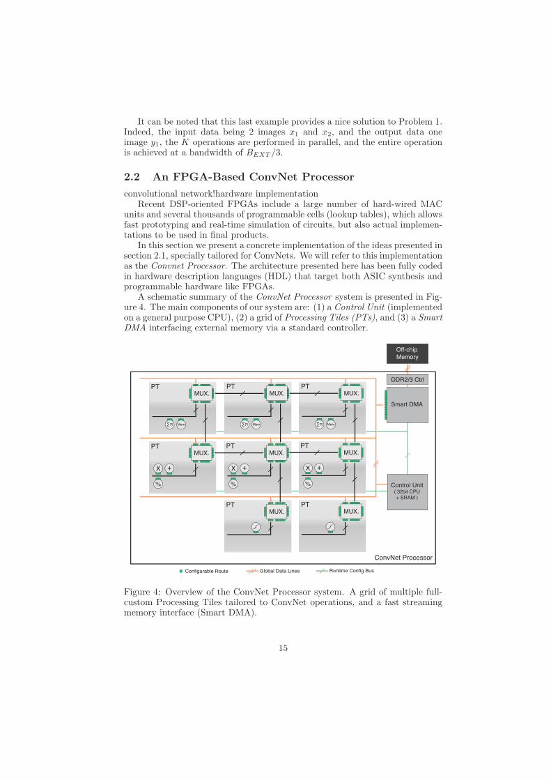
2.2 An FPGA-Based ConvNet Processor

convolutional network!hardware implementationRecent DSP-oriented FPGAs include a large number of hard-wired MAC

units and several thousands of programmable cells (lookup tables), which allowsfast prototyping and real-time simulation of circuits, but also actual implemen-tations to be used in final products.

In this section we present a concrete implementation of the ideas presented insection 2.1, specially tailored for ConvNets. We will refer to this implementationas the Convnet Processor. The architecture presented here has been fully codedin hardware description languages (HDL) that target both ASIC synthesis andprogrammable hardware like FPGAs.

A schematic summary of the ConvNet Processor system is presented in Fig-ure 4. The main components of our system are: (1) a Control Unit (implementedon a general purpose CPU), (2) a grid of Processing Tiles (PTs), and (3) a SmartDMA interfacing external memory via a standard controller.

MUX.

X +

%

MUX.

MUX.

∑π

MUX.

X +

%

MUX.

X +

%

MUX.

MUX. MUX.

Control Unit( 32bit CPU

+ SRAM )

Smart DMA

Configurable Route Global Data Lines Runtime Config Bus

Off-chip

Memory

Mem∑π Mem∑π Mem

ConvNet Processor

PT PT PT

PTPTPT

PT PT

DDR2/3 Ctrl

Figure 4: Overview of the ConvNet Processor system. A grid of multiple full-custom Processing Tiles tailored to ConvNet operations, and a fast streamingmemory interface (Smart DMA).

15

In this implementation, the Control Unit is implemented by a general purposeCPU. This is more convenient than a custom state machine as it allows the useof standard C compilers. Moreover, the CPU has full access to the externalmemory (via global data lines), and it can use this large storage to store itsprogram instructions.

2.2.1 Specialized Processing Tiles

The PTs are independent processing tiles laid out on a two-dimensional grid.As presented in section 2.1, they contain a routing multiplexer (MUX) andlocal operators. Compared to the general purpose architecture proposed above,this implementation is specialized for ConvNets and other applications that relyheavily on two-dimensional convolutions (from 80% to 90% of computations forConvNets).

Figure 4 shows this specialization:

• the top row PTs only implement Multiply and Accumulate (MAC) arrays(∑∏

operators), which can be used as 2D convolvers (implemented inthe FPGA by dedicated hardwired MACs). It can also perform on-the-fly subsampling (spatial pooling), and simple dot-products (linear classi-fiers) (Farabet et al., 2009),

• the middle row PTs contain general purpose operators (squaring and di-viding are necessary for divisive normalization),

• the bottom row PTs implement non-linear mapping engines, used to com-pute all sorts of functions from Tanh() to Sqrt() or Abs(). Those canbe used at all stages of the ConvNets, from normalization to non-linearactivation units.

The operators in the PTs are fully pipelined to produce one result per clockcycle. Image pixels are stored in off-chip memory as Q8.8 (16bit, fixed-point),transported on global lines as Q8.8 but scaled to 32bit integers within operators,to keep full precision between successive operations. The numeric precision, andhence the size of a pixel, will be noted Pbits.

The 2D convolver can be viewed as a data-flow grid itself, with the onlydifference that the connections between the operators (the MACs) are fixed.The reason for having a full-blown 2D convolver within a tile (instead of a 1Dconvolver per tile, or even simply one MAC per tile) is that it maximizes theratio between actual computing logic and routing logic, as stated previously.Of course it is not as flexible, and the choice of the array size is a hardwiredparameter, but it is a reasonable choice for an FPGA implementation, and forimage processing in general. For an ASIC implementation, having a 1D dot-product operator per tile is probably the best compromise.

The pipelined implementation of this 2D convolver (as described in Farabetet al. (2009)), computes Equation 8 at every clock cycle.

y1,i,j = x2,i,j +

K−1∑

m=0

K−1∑

n=0

x1,i+m,j+nw1,m,n (8)

16

In equation 8 x1,i,j is a value in the input plane, w1,m,n is a value in a K×Kconvolution kernel, x2,i,j is a value in a plane to be combined with the result,and y1 is the output plane.

Both the kernel and the image are streams loaded from the memory, and thefilter kernels can be pre-loaded in local caches concurrently to another operation:each new pixel thus triggers K ×K parallel operations.

All the non-linearities in neural networks can be computed with the use oflook-up tables or piece-wise linear decompositions.

A loop-up table associates one output value for each input value, and there-fore requires as much memory as the range of possible inputs. It is the fastestmethod to compute a non-linear mapping, but the time required to reload anew table is prohibitive if different mappings are to be computed with the samehardware.

A piece-wise linear decomposition is not as accurate (f is approximatedby g, as in Eq. 9), but only requires a couple of coefficients ai to representa simple mapping such as a hyperbolic tangent, or a square root. It can bereprogrammed very quickly at runtime, allowing multiple mappings to reusethe same hardware. Moreover, if the coefficients ai follow the constraint givenby Eq. 10, the hardware can be reduced to shifters and adders only.

g(x) = aix+ bi for x ∈ [li, li+1] (9)

ai =1

2m+

1

2nm,n ∈ [0, 5]. (10)

2.2.2 Smart DMA Implementation

A critical part of this architecture is the Direct Memory Access (DMA) module.Our Smart DMA module is a full custom engine that has been designed to allowNDMA ports to access the external memory totally asynchronously.

A dedicated arbiter is used as hardware Memory Interface to multiplex anddemultiplex access to the external memory with high bandwidth. Subsequentbuffers on each port insure continuity of service on a port while the others areutilized.

The DMA is smart, because it complements the Control Unit. Each port ofthe DMA can be configured to read or write a particular chunk of data, withan optional stride (for 2D streams), and communicate its status to the ControlUnit. Although this might seem trivial, it respects of one the foundations ofdata-flow computing: while the Control Unit configures the grid and the DMAports for each operation, an operation is driven exclusively by the data, fromits fetching, to its writing back to off-chip memory.

If the PTs are synchronous to the memory bus clock, the following relation-ship can be established between the memory bandwidth BEXT , the number ofpossible parallel data transfers MAX(NDMA) and the bits per pixel Pbits:

MAX(NDMA) =BEXT

Pbits. (11)

For example Pbits = 16 and BEXT = 128bit/cyc allows MAX(NDMA) = 7simultaneous transfers.

17

2.3 Compiling ConvNets for the ConvNet Processor

Prior to being run on the ConvNet Processor, a ConvNet has to be trainedoffline, on a regular computer, and then converted to a compact representationthat can be interpreted by the Control Unit to generate controls/configurationsfor the system.

Offline, the training is performed with existing software such as Lush (LeCunand Bottou, 2002) or Torch-5 (Collobert, 2008). Both libraries use the modularapproach described in the introduction of section 2.

On board, the Control Unit of the ConvNet Processor decodes the repre-sentation, which results in several grid reconfigurations, interspersed with datastreams. This representation will be denoted as bytecode from now on. Com-piling a ConvNet for the ConvNet Processor can be summarized as the task ofmapping the offline training results to this bytecode.

Extensive research has been done on the question of how to schedule data-flow computations (Lee and David, 1987), and how to represent streams andcomputations on streams (l. Gaudiot et al., 1994). In this section, we only careabout how to schedule computations for a ConvNet (and similar architectures)on our ConvNet Processor engine.

It is a more restricted problem, and can be stated simply:

Problem 3. Given a particular ConvNet architecture, and trained parameters,and given a particular implementation of the data-flow grid, what is the sequenceof grid configurations that yield the shortest computation time? Or in otherterms, for a given ConvNet architecture, and a given data-flow architecture,how to produce the bytecode that yields the shortest computing time?

As described in the introduction of section 2, there are three levels at whichcomputations can be parallelized:

• across modules: operators can be cascaded, and multiple modules can becomputed on the fly (average speedup),

• across images, within a module: can be done if multiple instances of therequired operator exist (poor speedup, as each independent operation re-quires its own input/output streams, which are limited by BEXT ),

• within an image: some operators naturally implement that (the 2D con-volver, which performs all the MACs in parallel), in some cases, multipletiles can be used to parallelize computations.

Parallelizing computations across modules can be done in special cases. Ex-ample 2 illustrates this case: two operators (each belonging to a separate mod-ule) are cascaded, which speeds up this computation by a factor of 2.

Parallelizing computations across images is straightforward but very limited.Here is an example that illustrates that point:

Example 4. The data-flow system built has 3 PTs with 2D convolvers, 3 PTswith standard operators, and 2 PTs with non-linear mappers (as depicted inFigure 4, and the exercise is to map a fully-connected filter-bank with 3 inputsand 8 outputs, e.g. a filer bank where each of the 8 outputs is a sum of 3 inputsconvolved with a different kernel:

18

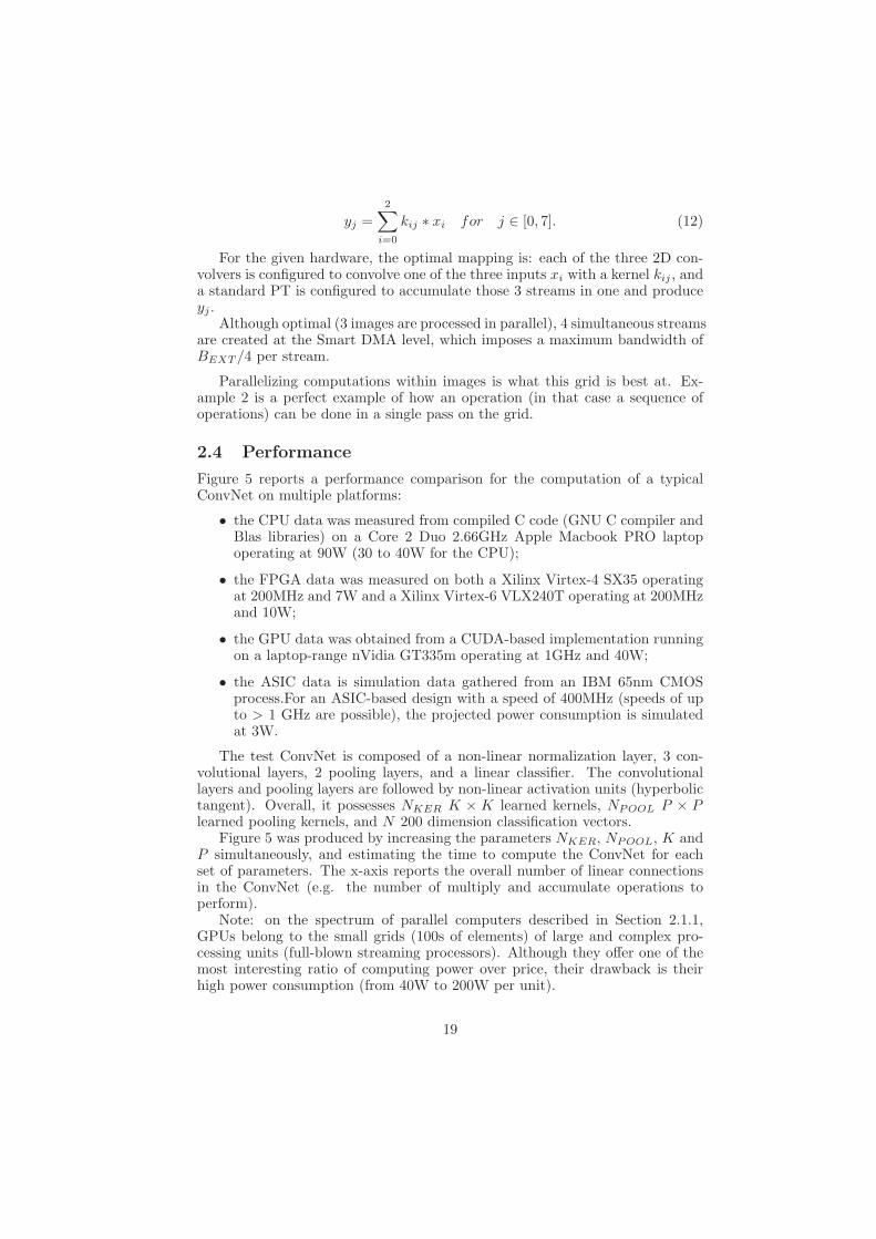
yj =2∑

i=0

kij ∗ xi for j ∈ [0, 7]. (12)

For the given hardware, the optimal mapping is: each of the three 2D con-volvers is configured to convolve one of the three inputs xi with a kernel kij , anda standard PT is configured to accumulate those 3 streams in one and produceyj .

Although optimal (3 images are processed in parallel), 4 simultaneous streamsare created at the Smart DMA level, which imposes a maximum bandwidth ofBEXT /4 per stream.

Parallelizing computations within images is what this grid is best at. Ex-ample 2 is a perfect example of how an operation (in that case a sequence ofoperations) can be done in a single pass on the grid.

2.4 Performance

Figure 5 reports a performance comparison for the computation of a typicalConvNet on multiple platforms:

• the CPU data was measured from compiled C code (GNU C compiler andBlas libraries) on a Core 2 Duo 2.66GHz Apple Macbook PRO laptopoperating at 90W (30 to 40W for the CPU);

• the FPGA data was measured on both a Xilinx Virtex-4 SX35 operatingat 200MHz and 7W and a Xilinx Virtex-6 VLX240T operating at 200MHzand 10W;

• the GPU data was obtained from a CUDA-based implementation runningon a laptop-range nVidia GT335m operating at 1GHz and 40W;

• the ASIC data is simulation data gathered from an IBM 65nm CMOSprocess.For an ASIC-based design with a speed of 400MHz (speeds of upto > 1 GHz are possible), the projected power consumption is simulatedat 3W.

The test ConvNet is composed of a non-linear normalization layer, 3 con-volutional layers, 2 pooling layers, and a linear classifier. The convolutionallayers and pooling layers are followed by non-linear activation units (hyperbolictangent). Overall, it possesses NKER K × K learned kernels, NPOOL P × Plearned pooling kernels, and N 200 dimension classification vectors.

Figure 5 was produced by increasing the parameters NKER, NPOOL, K andP simultaneously, and estimating the time to compute the ConvNet for eachset of parameters. The x-axis reports the overall number of linear connectionsin the ConvNet (e.g. the number of multiply and accumulate operations toperform).

Note: on the spectrum of parallel computers described in Section 2.1.1,GPUs belong to the small grids (100s of elements) of large and complex pro-cessing units (full-blown streaming processors). Although they offer one of themost interesting ratio of computing power over price, their drawback is theirhigh power consumption (from 40W to 200W per unit).

19

6 8 10 12 14 16 18 20 22# connections (x109 )

101

102

103

104

105

tim

e (

ms)

FPGA (Virtex4, 200MHz)

FPGA (Virtex6, 200MHz)

ASIC (IBM65nm, 400MHz)

GPU (GT335m, 1GHz)

CPU (DuoCore2, 2.6GHz)

Figure 5: Compute time for a typical ConvNet (as seen in Figure 1).

2.4.1 Precision

Recognition rates for standard datasets were obtained to benchmark the preci-sion loss induced by the fixed-point coding. Using floating-point representationfor training and testing, the following results were obtained: for NORB, 85%recognition rate was achieved on the test dataset, for MNIST, 95% and forUMASS (faces dataset), 98%. The same tests were conducted on the ConvNetProcessor with fixed-point representation (Q8.8), and the results were, respec-tively: 85%, 95% and 98%, which confirms the assumptions made a priori onthe influence of quantization noise.

To provide more insight into the fixed-point conversion, the number ofweights being zeroed with quantization was measured, in the case of the NORBobject detector. Figure 6 shows the results: at 8bits, the quantization impactis already significant (10% of weights become useless), although it has no effecton the detection accuracy.

3 Summary

The convolutional network architecture is a remarkably versatile, yet concep-tually simple paradigm that can be applied to a wide spectrum of perceptualtasks. While traditional ConvNets trained with supervised learning are veryeffective, training them requires a large number of labeled training samples.We have shown that using simple architectural tricks such as rectification and

20

21

0 5 10 15 20 25 30 35Fixed point position

0

20

40

60

80

100

Perc

enta

ge o

f w

eig

hts

zero

ed

Figure 6: Quantization effect on trained networks: the x axis shows the fixedpoint position, the y axis the percentage of weights being zeroed after quanti-zation.

contrast normalization, and using unsupervised pre-training of each filter bank,the need for labeled samples is considerably reduced.

We presented a data-flow computer that can be optimized to compute con-volutional networks. Different use cases were studied, and it was seen thatmapping/unrolling a convolutional network was straight-forward on such anarchitecture, thanks to their relatively uniform design.

Because of their applicability to a wide range of tasks, ConvNets are per-fect candidates for hardware implementations, and embedded applications, asdemonstrated by the increasing amount of work in this area. We expect to seemany new embedded vision systems based on ConvNets in the next few years.

Future work on our data-flow architecture will aim at making it more gen-eral, to open the doors to more complex and generic recognition tasks. Multipleobject detection (LeCun et al., 2004) or online learning for adaptive robot guid-ance (Hadsell et al., 2009) are tasks that will be largely improved by this system.

22

References

Adams, Duane Albert. 1969. A computation model with data flow sequencing.Ph.D. thesis, Stanford, CA, USA.

Ahmed, Amr, Yu, Kai, Xu, Wei, Gong, Yihong, and Xing, Eric. 2008. TrainingHierarchical Feed-Forward Visual Recognition Models Using Transfer Learn-ing from Pseudo-Tasks. In: ECCV. Springer-Verlag.

Bengio, Yoshua, Lamblin, Pascal, Popovici, Dan, and Larochelle, Hugo. 2007.Greedy Layer-Wise Training of Deep Networks. In: NIPS.

Berg, A. C., Berg, T. L., and Malik, J. 2005. Shape Matching and ObjectRecognition Using Low Distortion Correspondences. In: CVPR.

Chellapilla, Kumar, Shilman, Michael, and Simard, Patrice. 2006. Optimallycombining a cascade of classifiers. In: Proc. of Document Recognition andRetrieval 13, Electronic Imaging, 6067.

Cho, Myong Hyon, chi Cheng, Chih, Kinsy, Michel, Suh, G. Edward, and De-vadas, Srinivas. 2008. Diastolic Arrays: Throughput-Driven ReconfigurableComputing.

Coates, A., Baumstarck, P., Le, Q., and Ng, A.Y. 2009. Scalable learning forobject detection with GPU hardware. Pages 4287–4293 of: Proceedings of the2009 IEEE/RSJ international conference on Intelligent robots and systems.Citeseer.

Collobert, R. 2008. Torch. presented at the Workshop on Machine LearningOpen Source Software, NIPS.

Dalal, Navneet, and Triggs, Bill. 2005. Histograms of Oriented Gradients forHuman Detection. In: CVPR.

Delakis, M., and Garcia, C. 2008. Text Detection with Convolutional NeuralNetworks. In: International Conference on Computer Vision Theory andApplications (VISAPP 2008).

Dennis, Jack B., and Misunas, David P. 1974. A preliminary architecture for abasic data-flow processor. SIGARCH Comput. Archit. News, 3(4), 126–132.

Farabet, Clement, Poulet, Cyril, Han, Jefferson Y., and LeCun, Yann. 2009.CNP: An FPGA-based Processor for Convolutional Networks. In: Interna-tional Conference on Field Programmable Logic and Applications (FPL’09).Prague: IEEE.

Farabet, Clement, Martini, Berin, Akselrod, Polina, Talay, Selcuk, LeCun,Yann, and Culurciello, Eugenio. 2010. Hardware Accelerated ConvolutionalNeural Networks for Synthetic Vision Systems. In: International Symposiumon Circuits and Systems (ISCAS’10). Paris: IEEE.

Frome, A, Cheung, G, Abdulkader, A., Zennaro, M., Wu, B., Bissacco, A.,Adam, H., Neven, H., and Vincent, L. 2009. Large-Scale Privacy Protectionin Street-Level Imagery. In: ICCV’09.

23

Fukushima, Kunihiko, and Miyake, Sei. 1982. Neocognitron: A new algorithmfor pattern recognition tolerant of deformations and shifts in position. PatternRecognition, 15(6), 455–469.

Garcia, C., and Delakis, M. 2004. Convolutional Face Finder: A Neural Archi-tecture for Fast and Robust Face Detection. IEEE Transactions on PatternAnalysis and Machine Intelligence.

Hadsell, Raia, Sermanet, Pierre, Scoffier, Marco, Erkan, Ayse, Kavackuoglu,Koray, Muller, Urs, and LeCun, Yann. 2009. Learning Long-Range Vision forAutonomous Off-Road Driving. Journal of Field Robotics, 26(2), 120–144.

Hicks, James, Chiou, Derek, Ang, Boon Seong, and Arvind. 1993. PerformanceStudies of Id on the Monsoon Dataflow System.

Hinton, G E, and Salakhutdinov, R R. 2006. Reducing the dimensionality ofdata with neural networks. Science.

Huang, Fu-Jie, and LeCun, Yann. 2006. Large-Scale Learning with SVM andConvolutional Nets for Generic Object Categorization. In: Proc. ComputerVision and Pattern Recognition Conference (CVPR’06). IEEE Press.

Jain, Viren, and Seung, H. Sebastian. 2008. Natural Image Denoising with Con-volutional Networks. In: Advances in Neural Information Processing Systems21 (NIPS 2008). MIT Press.

Jarrett, Kevin, Kavukcuoglu, Koray, Ranzato, Marc’Aurelio, and LeCun, Yann.2009. What is the Best Multi-Stage Architecture for Object Recognition? In:Proc. International Conference on Computer Vision (ICCV’09). IEEE.

Kavukcuoglu, Koray, Ranzato, Marc’Aurelio, and LeCun, Yann. 2008. Fast In-ference in Sparse Coding Algorithms with Applications to Object Recognition.Tech. rept. Tech Report CBLL-TR-2008-12-01.

Kavukcuoglu, Koray, Ranzato, Marc’Aurelio, Fergus, Rob, and LeCun, Yann.2009. Learning Invariant Features through Topographic Filter Maps. In:Proc. International Conference on Computer Vision and Pattern Recognition(CVPR’09). IEEE.

Kung, H T. 1986. Why systolic architectures? 300–309.

l. Gaudiot, J., Bic, L., Dennis, Jack, and Dennis, Jack B. 1994. Stream DataTypes for Signal Processing. In: In Advances in Dataflow Architecture andMultithreading. IEEE Computer Society Press.

Lazebnik, S., Schmid, C., and Ponce, J. 2006. Beyond Bags of Features: SpatialPyramid Matching for Recognizing Natural Scene Categories. Pages 2169–2178 of: Proc. of Computer Vision and Pattern Recognition. IEEE.

LeCun, Y., and Bottou, L. 2002. Lush Reference Manual. Tech. rept. codeavailable at http://lush.sourceforge.net.

24

LeCun, Y., Boser, B., Denker, J. S., Henderson, D., Howard, R. E., Hubbard,W., and Jackel, L. D. 1989. Backpropagation Applied to Handwritten ZipCode Recognition. Neural Computation.

LeCun, Y., Boser, B., Denker, J. S., Henderson, D., Howard, R. E., Hubbard,W., and Jackel, L. D. 1990. Handwritten digit recognition with a back-propagation network. In: NIPS’89.

LeCun, Y., Bottou, L., Orr, G., and Muller, K. 1998a. Efficient BackProp. In:Orr, G., and K., Muller (eds), Neural Networks: Tricks of the trade. Springer.

LeCun, Y., Bottou, L., Bengio, Y., and Haffner, P. 1998b. Gradient-BasedLearning Applied to Document Recognition. Proceedings of the IEEE, 86(11),2278–2324.

LeCun, Yann, and Cortes, Corinna. 1998. MNIST dataset.http://yann.lecun.com/exdb/mnist/.

LeCun, Yann, Huang, Fu-Jie, and Bottou, Leon. 2004. Learning Methods forGeneric Object Recognition with Invariance to Pose and Lighting. In: Pro-ceedings of CVPR’04. IEEE Press.

Lee, Edward Ashford, and David. 1987. Static Scheduling of Synchronous DataFlow Programs for Digital Signal Processing. IEEE Transactions on Com-puters, 36, 24–35.

Lee, Honglak, Grosse, Roger, Ranganath, Rajesh, and Ng, Andrew, Y. 2009.Convolutional deep belief networks for scalable unsupervised learning of hi-erarchical representations. In: Proc. of the 26th International Conference onMachine Learning (ICML’09).

Lowe, David G. 2004. Distinctive Image Features from Scale-Invariant Key-points. International Journal of Computer Vision.

Lyu, S, and Simoncelli, E P. 2008. Nonlinear image representation using divisivenormalization. In: CVPR.

Mozer, M.C. 1991. The Perception of Multiple Objects, A Connectionist Ap-proach. MIT Press.

Mutch, Jim, and Lowe, David G. 2006. Multiclass Object Recognition withSparse, Localized Features. In: CVPR.

Nasse, Fabian, Thurau, Christian, and Fink, Gernot A. 2009. Face detectionusing GPU-based convolutional neural networks.

Ning, Feng, Delhomme, Damien, LeCun, Yann, Piano, Fabio, Bottou, Leon,and Barbano, Paolo. 2005. Toward Automatic Phenotyping of DevelopingEmbryos from Videos. IEEE Transactions on Image Processing. Special issueon Molecular and Cellular Bioimaging.

Nowlan, S., and Platt, J. 1995. A Convolutional Neural Network Hand Tracker.Pages 901–908 of: Neural Information Processing Systems. San Mateo, CA:Morgan Kaufmann.

25

Olshausen, B A, and Field, D J. 1997. Sparse coding with an overcomplete basisset: a strategy employed by V1? Vision Research.

Osadchy, M., LeCun, Y., and Miller, M. 2007. Synergistic Face Detection andPose Estimation with Energy-Based Models. Journal of Machine LearningResearch, 8(May), 1197–1215.

Pinto, Nicolas, Cox, David D, and DiCarlo, James J. 2008. Why is Real-WorldVisual Object Recognition Hard? PLoS Comput Biol, 4(1), e27.

Ranzato, Marc’Aurelio, Boureau, Y-Lan, and LeCun, Yann. 2007a. Sparsefeature learning for deep belief networks. In: NIPS’07.

Ranzato, Marc’Aurelio, Huang, Fu-Jie, Boureau, Y-Lan, and LeCun, Yann.2007b. Unsupervised Learning of Invariant Feature Hierarchies with Ap-plications to Object Recognition. In: Proc. Computer Vision and PatternRecognition Conference (CVPR’07). IEEE Press.

Serre, Thomas, Wolf, Lior, and Poggio, Tomaso. 2005. Object Recognition withFeatures Inspired by Visual Cortex. In: CVPR.

Simard, Patrice, Y., Steinkraus, Dave, and Platt, John C. 2003. Best Practicesfor Convolutional Neural Networks Applied to Visual Document Analysis. In:ICDAR.

Vaillant, R., Monrocq, C., and LeCun, Y. 1994. Original approach for thelocalisation of objects in images. IEE Proc on Vision, Image, and SignalProcessing, 141(4), 245–250.

Weston, J., Rattle, F., and Collobert, R. 2008. Deep Learning via Semi-Supervised Embedding. In: ICML.

26