Large Scale Measurement and Characterization of Cellular ...alexliu/publications/M2M/Main_ToN_MSU.pdf · Large Scale Measurement and Characterization of ... To answer this question,

1

Large Scale Measurement and Characterization ofCellular Machine-to-Machine Traffic

M. Zubair Shafiq, Lusheng Ji, Alex X. Liu∗, Jeffrey Pang, and Jia Wang

Abstract—Cellular network based Machine-to-Machine (M2M)communication is fast becoming a market-changing force for awide spectrum of businesses and applications such as telematics,smart metering, point-of-sale terminals, and home security andautomation systems. In this paper, we aim to answer the followingimportant question: Does traffic generated by M2M devices im-pose new requirements and challenges for cellular network designand management? To answer this question, we take a first look atthe characteristics of M2M traffic and compare it with traditionalsmartphone traffic. We have conducted our measurement analysisusing a week-long traffic trace collected from a tier-1 cellularnetwork in the United States. We characterize M2M traffic froma wide range of perspectives, including temporal dynamics, devicemobility, application usage, and network performance.

Our experimental results show that M2M traffic exhibits sig-nificantly different patterns than smartphone traffic in multipleaspects. For instance, M2M devices have a much larger ratio ofuplink to downlink traffic volume, their traffic typically exhibitsdifferent diurnal patterns, they are more likely to generatesynchronized traffic resulting in bursty aggregate traffic volumes,and are less mobile compared to smartphones. On the other hand,we also find that M2M devices are generally competing withsmartphones for network resources in co-located geographicalregions. These and other findings suggest that better protocoldesign, more careful spectrum allocation, and modified pricingschemes may be needed to accommodate the rise of M2M devices.

I. INTRODUCTION

Smart devices that function without direct human interven-tion are rapidly becoming an integral part of our lives. Suchdevices are increasingly used in applications such as telehealth,shipping and logistics, utility and environmental monitoring,industrial automation, and asset tracking. Compared to tra-ditional automation technologies, one major difference forthis new generation of smart devices is how tightly they arecoupled into larger scale service infrastructures. For example,in logistic operations, the locations of fleet vehicles can betracked with Automatic Vehicle Location (AVL) devices suchas the CalAmp LMU-2600 [6] and uploaded into back-end au-tomatic dispatching and planning systems for real-time globalfleet management. More and more emerging technologies alsoheavily depend on these smart devices. For instance, a cornerstone for the Smart Grid Initiative is the capability of receiving

The preliminary version of this paper titled “A First Look at CellularMachine-to-Machine Traffic – Large Scale Measurement and Characteri-zation” was published in the proceedings of the ACM International Con-ference on Measurement and Modeling of Computer Systems (SIGMET-RICS/Performance), London, UK, June, 2012.∗ Alex X. Liu is the corresponding author of this paper.M. Zubair Shafiq and Alex X. Liu are with the Department of Computer

Science and Engineering, Michigan State University, East Lansing, MI, USA.Email: {shafiqmu,alexliu}@cse.msu.edu.

Lusheng Ji, Jeffrey Pang, and Jia Wang are with AT&T Labs – Research,Florham Park, NJ, USA. Email:{lji,jeffpang,jiawang}@research.att.com

and controlling individual customer’s power usage on a real-time and wide-area basis through devices such as the electricmeters equipped with Trilliant CellReader [24] modules.

This kind of leap in technology would not be possiblewithout the support of wide area wireless communication in-frastructure, in particular cellular data networks. It is estimatedthat there are already tens of millions of such smart devicesconnected to cellular networks world wide and within thenext 3-5 years this number will grow to hundreds of millions[2], [3]. This represents a substantial growth opportunity forcellular operators as the increase in mobile phone penetrationrate is flattening in the developed world [11], [25].

M2M devices and smartphones share the same networkinfrastructure, but current cellular data networks are primarilydesigned, engineered, and managed for smartphone usage.Given that the population of cellular M2M devices may sooneclipse that of smartphones, a logical question to ask is: Whatare the challenges that cellular network operators may facein trying to accommodate traffic from both smartphones andM2M devices? Existing configurations may not be optimizedto support M2M devices. In addition, M2M devices maycompete with smartphones and impose new demand on sharedresources. Hence, to answer this question, it is crucial tounderstand M2M traffic patterns and how they are differentfrom traditional smartphone traffic. The knowledge of trafficpatterns can reveal insights for better management of sharednetwork resources and ensuring best service quality for bothtypes of devices.

In this paper, we take a first look at M2M traffic on acommercial cellular network. Our goal is to understand thecharacteristics of M2M traffic, in particular, whether and howthey differ from those of smartphones. To the best of ourknowledge, our study is the first to investigate the charac-teristics of traffic generated by M2M devices. We summarizeour key contributions below.• Large Scale Measurement: We conduct the first largescale measurement study of cellular M2M traffic. For ourstudy, we have collected anonymized IP-level traffic tracesfrom the core network of a tier-1 cellular network in theUnited States. This trace covers all states in the UnitedStates during one week in August 2010. This trace containsM2M traffic from millions of devices belonging to more than150 hardware models. In addition, we have also collectedanonymized traffic traces from millions of smartphones fromthe same cellular network. Overall, we find that M2M devicesgenerate significantly less traffic compared to smartphones.Furthermore, in our trace, we observe that the number ofM2M devices is also significantly smaller than the number of

2

smartphones. However, the number of new M2M devices andtheir total traffic volume is increasing at a very rapid pace. Infact, a longitudinal comparison of M2M traffic in this cellularnetwork showed that total M2M traffic volume has increasedmore than 250% in 2011 since previous year. In comparison,Cisco reported that mobile data traffic grew “only” 132%in 2011, which is almost half of the increase observed forM2M traffic [4]. Consequently, it is important to understandthe peculiarities of M2M traffic, especially its contrast to thetraditional smartphone traffic, for future network engineering.In this study, we compare M2M and smartphone traffic inthe following aspects: aggregate volume, volume time series,sessions, mobility, applications, and network performance.• Aggregate Traffic Volume: We jointly study the distribu-tions of aggregate uplink and downlink traffic volume. Ourmajor finding is that, though M2M devices do not generate asmuch traffic as smartphones, they have a much larger ratio ofuplink to downlink traffic volume compared to smartphones.Since existing cellular data protocols support higher capacityin the downlink than the uplink, our finding suggests that net-work operators need careful spectrum allocation and manage-ment to avoid contention between low volume, uplink-heavyM2M traffic and high volume, downlink-heavy smartphonetraffic.• Traffic Volume Time Series: We analyze the traffic volumetime series of M2M devices and smartphones. Our analysisshows that different M2M device models exhibit differentdiurnal behaviors than smartphones. However, some M2Mdevice models do share similar peak hours as smartphones.Hence, M2M traffic imposes new requirements on the sharednetwork resources that need to be considered in capacity plan-ning, where network is usually provisioned according to peakusage. Another finding from time series analysis is that someM2M device models generate traffic in a synchronized fashion(like a botnet [23]), which can result in denial of service dueto limited radio spectrum. Therefore, M2M protocols shouldrandomize such network usage to avoid congesting the radionetwork.• Traffic Sessions: To understand the usage behavior ofindividual devices, we conduct session-level traffic analysisin terms of active time, session length, and session inter-arrival time. We find that high traffic volume does not alwayscorrelate with more active time. This finding calls for newbilling schemes, which go beyond per-byte charging models.We also find that M2M devices have different session lengthand inter-arrival time characteristics compared to smartphones.This finding can be utilized by device manufacturers to improvebattery management and by network operators to optimizeradio network parameters for M2M devices.• Device Mobility: We compare the mobility characteristicsof M2M devices and smartphones from both device andnetwork perspectives. We find that M2M devices, with afew exceptions, are less mobile than smartphones. We alsofind that M2M and smartphone traffic competes for networkresources in co-located geographical regions. This findingindicates that careful network resource allocation is requiredto avoid contention between low-volume M2M traffic and high-volume smartphone traffic.

• Application Usage: We also study the contribution ofdifferent applications to the aggregate traffic volume of M2Mdevices and smartphones. We find that M2M traffic mostlyuses custom application protocols for specific needs, whichis undesirable because it is difficult for network operators tounderstand and mitigate adverse effects from these protocolscompared to standard protocols.• Network Performance: The network performance resultsof M2M traffic, in terms of packet loss ratio and round triptime, show strong dependency on device radio technology(2G or 3G) and expected device environment (e.g. indoorsvs. outdoors). This implies that network operators will needto be cognizant of a large population of M2M devices onlegacy networks even as they re-provision spectrum for 4Gtechnologies to support newer smartphones.

The rest of this paper proceeds as follows. We first providedetails of our collected trace in Section II. Sections III–VIIIpresent measurement analysis of M2M and smartphone traffic.Finally, we conclude in Section IX.

II. DATAA. Data Set

The data used in this study is collected from a nation-widecellular network operator in the United States that provides2G and 3G cellular data services. It supports GPRS, EDGE,UMTS, and HSPA technologies. Architecturally, the portionof its network that supports cellular data service is organizedin two tiers. The lower tier, the radio access network, provideswireless connectivity to user devices, and the upper tier, thecore network, interfaces the cellular data network with theInternet. More details about cellular data network architecturecan be found in [21].

The data collection apparatus that produced the trace usedin our study is deployed at all links between Serving GatewaySupport Nodes (SGSN) and Gateway GRPS Support Nodes(GGSN) in the core network. This apparatus is capable ofanonymously logging session level traffic information at 5minute intervals for all IP data traffic between cellular devicesand the Internet. In other words, each record in the trace isa 5-minute traffic volume (i.e., TCP payload size in bytes)summary aggregated by unique device identifier and applica-tion category. Each record also contains the cell location ofthe device at the start of the session. Each record is originallytimestamped according to the standard coordinated universaltime (UTC), which is then converted to the local time atthe device for our analysis. This trace was collected duringone complete week in August 2010. Geographically, the tracecovers the whole United States.

Applications are identified using a combination of portinformation, HTTP host and user-agent information, and otherheuristics. Overall, traffic is classified into the following17 categories: (1) appstore, (2) jabber, (3) mms, (4)navigation, (5) email, (6) ftp, (7) gaming, (8) im,(9) miscellaneous, (10) optimization, (11) p2p, (12)apps, (13) streaming, (14) unknown, (15) voip, (16)vpn, and (17) web. POP3 and IMAP traffic is classifiedas email. Additional control channel information is usedto identify voip traffic. Most HTTP traffic is classified as

3

streaming or web based on mime type. Some heuristicsare employed to identify non-HTTP p2p traffic. Gnutella andBitTorrent tracker-based HTTP traffic is also labeled p2p.User-agent information is used to identify specific mobileapp traffic such as appstore. Port number informationis used to identify other traffic classes. Many low volumeapplications are jointly labeled as miscellaneous. Theremaining unclassified traffic is labeled as unknown. Moreinformation about application classification can be found in[10], [20].

B. M2M Device Categorization

The data set contains traffic records for all cellular devices,so we first need to separate M2M devices from the rest.Furthermore, because M2M devices are usually developed forspecific applications, significant behavioral differences are ex-pected between M2M devices for different target applications.Thus, it is reasonable to sub-divide M2M devices into cate-gories based on their intended application to better understandthe unique traffic characteristics of different M2M categories.We start this process by identifying the hardware model ofeach cellular device using the device’s Type Allocation Code(TAC), which is part of the unique identifier of each cellulardevice. Although the records in our data set are anonymized,the TAC portion of the unique identifier is retained. Thus,the hardware model of each cellular device is obtained byconsulting the TAC database of the GSM Association.

Because there is no rigorous definition for M2M devices orstandard ways for determining their application categories, andmany devices have multiple uses, knowing the device model isnot sufficient for identifying a device with certainty as M2Mdevice nor for identifying its M2M category. Towards thisend, we adopt the device classification scheme of a majorcellular service provider as a base template for categorizingM2M devices [1]. To supplement and verify this template, wealso use public information such as production brochures andspecification sheets. In total, we have classified more than 150device models as M2M devices, and further divide them intothe following 6 categories.1) Asset Tracking: These M2M devices are used to remotelytrack objects like cargo containers and other shipments. Thesedevices are often coupled with other sensors for tasks liketemperature and pressure measurement. In our trace, about18% devices belong to this category.2) Building Security: These M2M devices are typically usedto manage door access and security cameras. In our trace,about 14% devices belong to this category.3) Fleet: These M2M devices are used to monitor vehiclelocations, arrivals, and departures and provide real-time accessto critical operational data for logistic service providers. In ourtrace, about 51% devices belong to this category.4) Miscellaneous (Misc.): These M2M devices are genericcellular communication modems with embedded system datainput and output ports such as serial, I2C, analog, and digital.They provide network connectivity for customized solutions.In our trace, about 9% devices belong to this category.5) Metering: These M2M devices are mostly used for remotemeasurement and monitoring in agricultural, environmental,

and energy applications. In our trace, about 6% devices belongto this category.6) Telehealth: These M2M devices are mostly used for remotemeasurement and monitoring in healthcare applications. In ourtrace, about 2% devices belong to this category.

We acknowledge that due to lack of more detailed usageinformation and ambiguity in device registry databases, ourclassification may contain some errors. To limit such errors,we try to be as conservative as possible when decidingwhether to include a M2M device model in our study. Forexample, cellular routers are generally excluded from thisstudy because the actual end devices behind these routerscannot be identified. For cellular modems and modules, weexclude models with data interfaces likely used by modernday computers such as USB, PCI Express, and miniPCI butkeep those with UART, SPI, and I2C interfaces. Note thatwe may miss some M2M devices in our analysis that arenot active and hence they do not not appear in our trace.For the sake of comparing M2M and typical human-generatedtraffic characteristics, we have also included in our study trafficrecords from a uniformly sampled set of smartphone models,covering millions of smartphone devices.

C. Data Set Characteristics

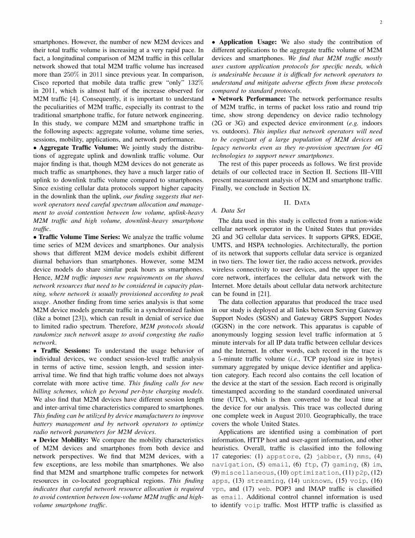
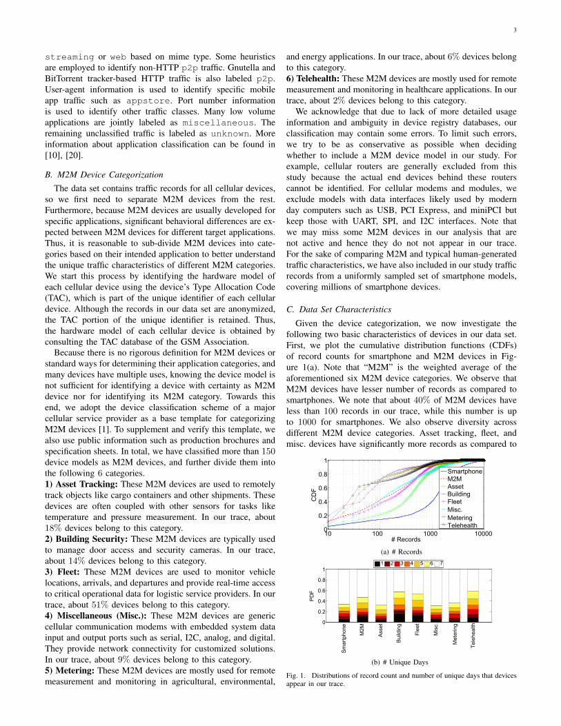
Given the device categorization, we now investigate thefollowing two basic characteristics of devices in our data set.First, we plot the cumulative distribution functions (CDFs)of record counts for smartphone and M2M devices in Fig-ure 1(a). Note that “M2M” is the weighted average of theaforementioned six M2M device categories. We observe thatM2M devices have lesser number of records as compared tosmartphones. We note that about 40% of M2M devices haveless than 100 records in our trace, while this number is upto 1000 for smartphones. We also observe diversity acrossdifferent M2M device categories. Asset tracking, fleet, andmisc. devices have significantly more records as compared to

100 1000 10000 100

0.2

0.4

0.6

0.8

1

# Records

CD

F

SmartphoneM2MAssetBuildingFleetMisc.MeteringTelehealth

(a) # Records

0

0.2

0.4

0.6

0.8

1

Sm

artp

hone

M2M

Ass

et

Bui

ldin

g

Flee

t

M

isc.

Met

erin

g

Tele

heal

th

PD

F

1 2 3 4 5 6 7

(b) # Unique Days

Fig. 1. Distributions of record count and number of unique days that devicesappear in our trace.

4

building, metering, and telehealth devices. M2M devices mayhave lesser number of records as compared to smartphonesbecause they often have one-off appearance in our trace.Second, to rule out the one-off appearance hypothesis, we plotthe probability distribution functions (PDFs) of the number ofunique days smartphone and M2M devices appear in our tracein Figure 1(b). We observe some differences across M2M de-vice categories; however, overall M2M and smartphones bothhave the most fraction of devices that appear on all days of theweek in our trace. Therefore, we can conclude that differencesobserved in Figure 1(a) are not simply because M2M devicesappear sporadically in our trace. The observations from thesetwo plots provide us a first evidence of difference in networkactivity of smartphone and M2M devices, and across M2Mdevice categories.

In the following sections, we conduct a detailed analysisand comparison of M2M and smartphone traffic characteristicsin our data set. The traffic characteristics analyzed in thispaper include aggregate data volume, volume time series,session analysis, mobility, application usage, and networkperformance. Note that some results presented in this paperare normalized by dividing with an arbitrary constant forproprietary reasons. However, normalization does not changethe range of the metrics used in this study. Furthermore,the missing information due to normalization does not affectthe understanding of our analysis. These characteristics arediscussed below in separate sections.

III. AGGREGATE TRAFFIC VOLUME

When a new technology emerges and it has to shareresources with existing parties, a natural first question is thelevel of competition and how different parties can better co-exist. This is why we first study and compare the distributionof aggregate traffic volume for M2M devices and smartphones.Moreover, we also investigate whether the long establishedperception of traffic volume being downlink heavy remainstrue for M2M devices [16].

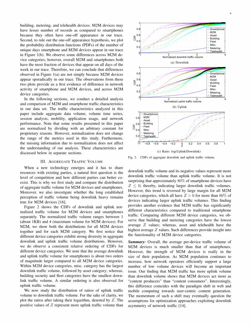
Figure 2 shows the CDFs of downlink and uplink nor-malized traffic volume for M2M devices and smartphonesseparately. The normalized traffic volume ranges between 1(about 1KB) and 4 (maximum volume for M2M devices). ForM2M, we show both the distributions for all M2M devicestogether and for each M2M category. We first notice thatdifferent device categories exhibit strong diversity in aggregatedownlink and uplink traffic volume distributions. However,we do observe a consistent relative ordering of CDFs fordifferent device categories. We note that the average downlinkand uplink traffic volume for smartphones is about two ordersof magnitude larger compared to all M2M device categories.Within M2M device categories, misc. category has the largestdownlink traffic volume, followed by asset category; whereas,building security and fleet categories have the smallest down-link traffic volume. A similar ordering is also observed foruplink traffic volume.

We now study the distribution of ratios of uplink trafficvolume to downlink traffic volume. For the sake of clarity, weplot the ratios after taking their logarithm, denoted by Z. Thepositive values of Z represent more uplink traffic volume than

1 2 3 40

0.2

0.4

0.6

0.8

1

Normalized downlink traffic volume

CD

F


(a) Downlink

1 2 3 40

0.2

0.4

0.6

0.8

1

Normalized uplink traffic volume

CD

F


(b) Uplink

−1 −0.8 −0.6 −0.4 −0.2 0 0.2 0.4 0.6 0.8 10

0.2

0.4

0.6

0.8

1

CD

F

Z


(c) Ratio: log(Uplink/Downlink)

Fig. 2. CDFs of aggregate downlink and uplink traffic volume.

downlink traffic volume and its negative values represent moredownlink traffic volume than uplink traffic volume. It is notsurprising that approximately 80% of smartphone devices haveZ ≤ 0; thereby, indicating larger downlink traffic volumes.However, this trend is reversed by large margin for all M2Mdevice categories, which all have Z > 0 for more than 80% ofdevices indicating larger uplink traffic volumes. This findingprovides another evidence that M2M traffic has significantlydifferent characteristics compared to traditional smartphonetraffic. Comparing different M2M device categories, we ob-serve that building and metering categories have the lowestaverage Z values; whereas, asset and telehealth have thehighest average Z values. Such differences provide insight intothe functionality of M2M device categories.

Summary: Overall, the average per-device traffic volume ofM2M devices is much smaller than that of smartphones.However, the strength of M2M devices is really in thesize of their population. As M2M population continues toincrease, how network operators efficiently support a largenumber of low volume devices will become an importantissue. Our finding that M2M traffic has more uplink volumethan downlink volume shows that M2M devices act more as“content producers” than “content consumers”. Interestingly,this difference coincides with the paradigm shift in web andmobile computing towards user-centric content generation.The momentum of such a shift may eventually question theassumptions for optimization approaches exploiting downlinkasymmetry of network traffic [14].

5

M Tu W Th F Sa Su0

0.2

0.4

0.6

0.8

1

Nor

mal

ized

Tra

ffic

Vol

ume

UplinkDownlink

(a) Smartphone

M Tu W Th F Sa Su0

0.2

0.4

0.6

0.8

1

Nor

mal

ized

Tra

ffic

Vol

ume

UplinkDownlink

(b) M2M

M Tu W Th F Sa Su0

0.2

0.4

0.6

0.8

1

Nor

mal

ized

Tra

ffic

Vol

ume

UplinkDownlink

(c) Asset

M Tu W Th F Sa Su0

0.2

0.4

0.6

0.8

1

Nor

mal

ized

Tra

ffic

Vol

ume

UplinkDownlink

(d) Building

M Tu W Th F Sa Su0

0.2

0.4

0.6

0.8

1

Nor

mal

ized

Tra

ffic

Vol

ume

UplinkDownlink

(e) Fleet

M Tu W Th F Sa Su0

0.2

0.4

0.6

0.8

1

Nor

mal

ized

Tra

ffic

Vol

ume

UplinkDownlink

(f) Misc.

M Tu W Th F Sa Su0

0.2

0.4

0.6

0.8

1

Nor

mal

ized

Tra

ffic

Vol

ume

UplinkDownlink

(g) Metering

M Tu W Th F Sa Su0

0.2

0.4

0.6

0.8

1

Nor

mal

ized

Tra

ffic

Vol

ume

UplinkDownlink

(h) Telehealth

Fig. 3. Downlink and uplink traffic volume time series.

IV. TRAFFIC VOLUME TIME SERIES

Having gained an understanding of aggregated M2M trafficvolume, we next study the temporal dynamics of M2M trafficvolume. It would be interesting to know whether M2M devicesexhibit similar daily diurnal pattern as smartphones. Oneparticular use of such information is to evaluate the potentialbenefits of incentive programs such as billing discounts en-couraging non-peak time usage. This information can also beutilized to group devices into separate clusters with differentbilling schemes. Time series analysis is also helpful for gaininginsights into the operations of M2M devices.

As mentioned in Section II, the logged traffic recordscontain timestamps at 5-minute time resolution. Therefore, wecan separately construct averaged traffic volume time seriesfor smartphones and all M2M device categories. We plotthese averaged uplink and downlink traffic volume time seriesin Figure 3. While the daily diurnal pattern is evident forboth M2M and smartphone traffic, the comparison of Figures3(a) and (b) reveals the following two interesting differences.First, the volume of downlink traffic dominates that of uplinktraffic for smartphones, whereas these are relatively samein M2M traffic time series. This finding follows our earlierobservations in Section III. Second, we also observe that peaksin smartphone traffic time series are wider, starting in themorning and prolonging up to mid-night, whereas peaks in

M2M traffic time series are narrower, ending by the eveningtime; and M2M traffic volume exhibits significant reductionduring weekend compared to weekdays while smartphonetraffic volume remains virtually unchanged. It appears thatsmartphone traffic time series is coupled with human “waking”hours while M2M traffic time series is coupled with human“working” hours. This is a strong indication that currently amajority of M2M devices are employed for business use. Theyare not yet in the mainstream for residential users, or as tightlyintegrated into people’s daily life as smartphones.

We have also separately plotted averaged uplink and down-link traffic volume time series for all M2M device categoriesin Figures 3(c)–(h). We observe strong diurnal variations forall M2M device categories. However, the weekday-weekendpattern comparison reveals different results for most M2Mcategories, illustrating that M2M categories indeed behavevastly differently from each other due to the different appli-cations they serve. The previously mentioned association ofM2M traffic time series with daily business activity cycle ishighlighted the most by Figure 3(d) (Building), where eachworking day pattern displays not only elevated volume duringworking hours but also two peaks which in time coincidewith the beginning and the end of typical business hours.Contrastingly, we see that there is virtually no difference intraffic volume for the metering category for different days.Frequency Analysis: On a finer scale, we observe repetitive

6

24 12 6 3 2 1 1/2 1/40

10

20

30

40

Time period (hours)

Pow

er/fr

eque

ncy

(dB

/Hz)

SmartphoneM2MMisc.Metering

(a) Downlink

24 12 6 3 2 1 1/2 1/40

10

20

30

40

Time period (hours)

Pow

er/fr

eque

ncy

(dB

/Hz)

SmartphoneM2MMisc.Metering

(b) Uplink

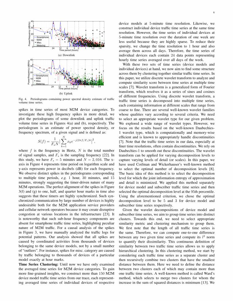
Fig. 4. Periodograms containing power spectral density estimate of trafficvolume time series.

spikes in time series of most M2M device categories. Toinvestigate these high frequency spikes in more detail, weplot the periodograms of some downlink and uplink trafficvolume time series in Figures 4(a) and (b), respectively. Theperiodogram is an estimate of power spectral density, orfrequency spectrum, of a given signal and is defined as:

S(f) =1

FsN

∣∣ N∑k=1

xke−j(2πf/Fs)k

∣∣2,where f is the frequency in Hertz, N is the total numberof signal samples, and Fs is the sampling frequency [22]. Inthis study, we have Fs = 5 minutes and N = 2, 016. The x-axis in Figure 4 represents time period on logarithm scale andy-axis represents power in decibels (dB) for each frequency.We observe distinct spikes in the periodograms correspondingto multiple time periods, e.g. 1 hour, 30 minutes, and 15minutes, strongly suggesting the timer-driven nature of manyM2M operations. The perfect alignment of the spikes in Figure3(f) and (g) to one, half, and quarter hour marks in time alsosuggests that these timers are highly synchronized. Such syn-chronized communication by large number of devices is highlyundesirable both for the M2M application service providersand cellular network operators because it may create disruptivecongestion at various locations in the infrastructure [23]. Itis noteworthy that such sub-hour frequency components areabsent for smartphone traffic time series, highlighting peculiarnature of M2M traffic. For a causal analysis of the spikesin Figure 3, we have manually analyzed the traffic logs forpotential patterns. Our analysis showed that all spikes arecaused by coordinated activities from thousands of devicesbelonging to the same device models, not by a small numberof “outliers”. For instance, spikes for misc. category are causedby traffic belonging to thousands of devices of a particularmodel exactly at hour marks.Time Series Clustering: Until now we have only examinedthe averaged time series for M2M device categories. To gainmore fine-grained insights, we construct more than 150 M2Mdevice model traffic time series from our trace, each represent-ing averaged time series of individual devices of respective

device models at 5-minute time resolution. Likewise, weconstruct individual device traffic time series at the same timeresolution. However, the time series of individual devices at5-minute time resolution over the duration of one week areless useful because they are highly sparse. To reduce theirsparsity, we change the time resolution to 1 hour and alsoaverage them across all days. Therefore, the time series ofindividual devices each contain 24 data points representinghourly time series averaged over all days of the week.

With these two sets of time series (device models andindividual devices) at hand, we now aim to find some structureacross them by clustering together similar traffic time series. Inthis paper, we utilize discrete wavelet transform to analyze andcompute similarity score between time series at multiple timescales [7]. Wavelet transform is a generalized form of Fouriertransform, which resolves it as a series of sines and cosinesof different frequencies. Using discrete wavelet transform, atraffic time series is decomposed into multiple time series,each containing information at different scales that range fromcoarse to fine. There are several well-known wavelet familieswhose qualities vary according to several criteria. We needto select an appropriate wavelet type for our given problem.We explored a wide range of wavelet types. However, wefocus on the results based on the well-known Daubechies-1 wavelet type, which is computationally and memory-wiseefficient and is known to appropriately handle discontinuities[7]. Note that the traffic time series in our data, especially atfiner time resolutions, often contain discontinuities. We rely onDaubechies-1 to smooth out these discontinuities. The wavelettransform can be applied for varying decomposition levels tocapture varying levels of detail (or scales). In this paper, wehave used Coifman and Wickerhauser’s well-known methodto select the optimal number of decomposition levels [8].The basic idea of this method is to select the decompositionlevel for which the joint information entropy of approximationand detail is minimized. We applied this method separatelyfor device model and subscriber traffic time series and thenselected the optimal decomposition level at the 95th percentile.Using the aforementioned criterion, we chose the optimaldecomposition level to be 5 and 3 for device model andsubscriber time series respectively.

Given the wavelet decompositions of device model andsubscriber time series, we aim to group time series into distinctclusters. Towards this end, we need to select appropriatesimilarity metric and clustering mechanism to group them.We first note that the length of all traffic time series isthe same. Therefore, we can compute one-to-one differencebetween any two given time series and compute its l2 normto quantify their dissimilarity. This continuous definition ofsimilarity between two traffic time series allows us to applyhierarchical clustering. In this clustering method, we start byconsidering each traffic time series as a separate cluster andthen recursively combine two clusters that have the smallestdistance between them. Here we need to define the distancebetween two clusters each of which may contain more thanone traffic time series. A well-known method is called Ward’smethod, which selects to merge two clusters for whom theincrease in the sum of squared distances is minimum [13]. We

7

0

5

10

15

20

25

30

35D

ista

nce

Index

(a) Device model

0

1

2

3

4

5

Dis

tanc

e

Index

(b) Individual device

Fig. 5. Dendrograms for hierarchical clustering.

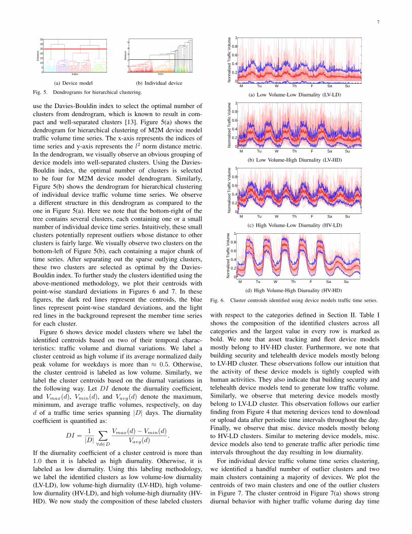
use the Davies-Bouldin index to select the optimal number ofclusters from dendrogram, which is known to result in com-pact and well-separated clusters [13]. Figure 5(a) shows thedendrogram for hierarchical clustering of M2M device modeltraffic volume time series. The x-axis represents the indices oftime series and y-axis represents the l2 norm distance metric.In the dendrogram, we visually observe an obvious grouping ofdevice models into well-separated clusters. Using the Davies-Bouldin index, the optimal number of clusters is selectedto be four for M2M device model dendrogram. Similarly,Figure 5(b) shows the dendrogram for hierarchical clusteringof individual device traffic volume time series. We observea different structure in this dendrogram as compared to theone in Figure 5(a). Here we note that the bottom-right of thetree contains several clusters, each containing one or a smallnumber of individual device time series. Intuitively, these smallclusters potentially represent outliers whose distance to otherclusters is fairly large. We visually observe two clusters on thebottom-left of Figure 5(b), each containing a major chunk oftime series. After separating out the sparse outlying clusters,these two clusters are selected as optimal by the Davies-Bouldin index. To further study the clusters identified using theabove-mentioned methodology, we plot their centroids withpoint-wise standard deviations in Figures 6 and 7. In thesefigures, the dark red lines represent the centroids, the bluelines represent point-wise standard deviations, and the lightred lines in the background represent the member time seriesfor each cluster.

Figure 6 shows device model clusters where we label theidentified centroids based on two of their temporal charac-teristics: traffic volume and diurnal variations. We label acluster centroid as high volume if its average normalized dailypeak volume for weekdays is more than ≈ 0.5. Otherwise,the cluster centroid is labeled as low volume. Similarly, welabel the cluster centroids based on the diurnal variations inthe following way. Let DI denote the diurnality coefficient,and Vmax(d), Vmin(d), and Vavg(d) denote the maximum,minimum, and average traffic volumes, respectively, on dayd of a traffic time series spanning |D| days. The diurnalitycoefficient is quantified as:

DI =1

|D|∑∀d∈D

Vmax(d)− Vmin(d)Vavg(d)

.

If the diurnality coefficient of a cluster centroid is more than1.0 then it is labeled as high diurnality. Otherwise, it islabeled as low diurnality. Using this labeling methodology,we label the identified clusters as low volume-low diurnality(LV-LD), low volume-high diurnality (LV-HD), high volume-low diurnality (HV-LD), and high volume-high diurnality (HV-HD). We now study the composition of these labeled clusters

M Tu W Th F Sa Su0

0.2

0.4

0.6

0.8

1

Nor

mal

ized

Tra

ffic

Vol

ume

(a) Low Volume-Low Diurnality (LV-LD)

M Tu W Th F Sa Su0

0.2

0.4

0.6

0.8

1

Nor

mal

ized

Tra

ffic

Vol

ume

(b) Low Volume-High Diurnality (LV-HD)

M Tu W Th F Sa Su0

0.2

0.4

0.6

0.8

1

Nor

mal

ized

Tra

ffic

Vol

ume

(c) High Volume-Low Diurnality (HV-LD)

M Tu W Th F Sa Su0

0.2

0.4

0.6

0.8

1N

orm

aliz

ed T

raffi

c V

olum

e

(d) High Volume-High Diurnality (HV-HD)

Fig. 6. Cluster centroids identified using device models traffic time series.

with respect to the categories defined in Section II. Table Ishows the composition of the identified clusters across allcategories and the largest value in every row is marked asbold. We note that asset tracking and fleet device modelsmostly belong to HV-HD cluster. Furthermore, we note thatbuilding security and telehealth device models mostly belongto LV-HD cluster. These observations follow our intuition thatthe activity of these device models is tightly coupled withhuman activities. They also indicate that building security andtelehealth device models tend to generate low traffic volume.Similarly, we observe that metering device models mostlybelong to LV-LD cluster. This observation follows our earlierfinding from Figure 4 that metering devices tend to downloador upload data after periodic time intervals throughout the day.Finally, we observe that misc. device models mostly belongto HV-LD clusters. Similar to metering device models, misc.device models also tend to generate traffic after periodic timeintervals throughout the day resulting in low diurnality.

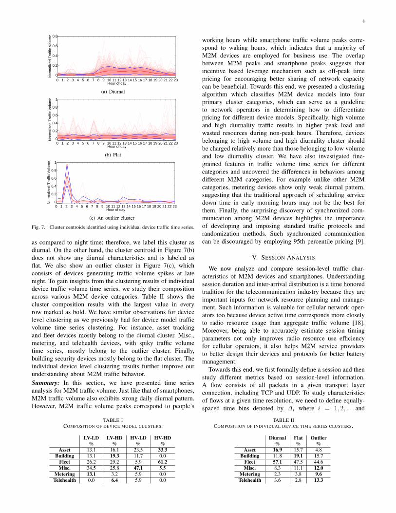
For individual device traffic volume time series clustering,we identified a handful number of outlier clusters and twomain clusters containing a majority of devices. We plot thecentroids of two main clusters and one of the outlier clustersin Figure 7. The cluster centroid in Figure 7(a) shows strongdiurnal behavior with higher traffic volume during day time

8

0 1 2 3 4 5 6 7 8 9 10 11 12 13 14 15 16 17 18 19 20 21 22 230

0.2

0.4

0.6

0.8

Nor

mal

ized

Tra

ffic

Vol

ume

Hour of day

(a) Diurnal

0 1 2 3 4 5 6 7 8 9 10 11 12 13 14 15 16 17 18 19 20 21 22 230

0.2

0.4

0.6

0.8

1

Nor

mal

ized

Tra

ffic

Vol

ume

Hour of day

(b) Flat

0 1 2 3 4 5 6 7 8 9 10 11 12 13 14 15 16 17 18 19 20 21 22 230

0.2

0.4

0.6

0.8

1

Nor

mal

ized

Tra

ffic

Vol

ume

Hour of day

(c) An outlier cluster

Fig. 7. Cluster centroids identified using individual device traffic time series.

as compared to night time; therefore, we label this cluster asdiurnal. On the other hand, the cluster centroid in Figure 7(b)does not show any diurnal characteristics and is labeled asflat. We also show an outlier cluster in Figure 7(c), whichconsists of devices generating traffic volume spikes at latenight. To gain insights from the clustering results of individualdevice traffic volume time series, we study their compositionacross various M2M device categories. Table II shows thecluster composition results with the largest value in everyrow marked as bold. We have similar observations for devicelevel clustering as we previously had for device model trafficvolume time series clustering. For instance, asset trackingand fleet devices mostly belong to the diurnal cluster. Misc.,metering, and telehealth devices, with spiky traffic volumetime series, mostly belong to the outlier cluster. Finally,building security devices mostly belong to the flat cluster. Theindividual device level clustering results further improve ourunderstanding about M2M traffic behavior.Summary: In this section, we have presented time seriesanalysis for M2M traffic volume. Just like that of smartphones,M2M traffic volume also exhibits strong daily diurnal pattern.However, M2M traffic volume peaks correspond to people’s

TABLE ICOMPOSITION OF DEVICE MODEL CLUSTERS.

LV-LD LV-HD HV-LD HV-HD% % % %

Asset 13.1 16.1 23.5 33.3Building 13.1 19.3 11.7 0.0

Fleet 26.2 29.2 5.9 61.2Misc. 34.5 25.8 47.1 5.5

Metering 13.1 3.2 5.9 0.0Telehealth 0.0 6.4 5.9 0.0

working hours while smartphone traffic volume peaks corre-spond to waking hours, which indicates that a majority ofM2M devices are employed for business use. The overlapbetween M2M peaks and smartphone peaks suggests thatincentive based leverage mechanism such as off-peak timepricing for encouraging better sharing of network capacitycan be beneficial. Towards this end, we presented a clusteringalgorithm which classifies M2M device models into fourprimary cluster categories, which can serve as a guidelineto network operators in determining how to differentiatepricing for different device models. Specifically, high volumeand high diurnality traffic results in higher peak load andwasted resources during non-peak hours. Therefore, devicesbelonging to high volume and high diurnality cluster shouldbe charged relatively more than those belonging to low volumeand low diurnality cluster. We have also investigated fine-grained features in traffic volume time series for differentcategories and uncovered the differences in behaviors amongdifferent M2M categories. For example unlike other M2Mcategories, metering devices show only weak diurnal pattern,suggesting that the traditional approach of scheduling servicedown time in early morning hours may not be the best forthem. Finally, the surprising discovery of synchronized com-munication among M2M devices highlights the importanceof developing and imposing standard traffic protocols andrandomization methods. Such synchronized communicationcan be discouraged by employing 95th percentile pricing [9].

V. SESSION ANALYSIS

We now analyze and compare session-level traffic char-acteristics of M2M devices and smartphones. Understandingsession duration and inter-arrival distribution is a time honoredtradition for the telecommunication industry because they areimportant inputs for network resource planning and manage-ment. Such information is valuable for cellular network oper-ators too because device active time corresponds more closelyto radio resource usage than aggregate traffic volume [18].Moreover, being able to accurately estimate session timingparameters not only improves radio resource use efficiencyfor cellular operators, it also helps M2M service providersto better design their devices and protocols for better batterymanagement.

Towards this end, we first formally define a session and thenstudy different metrics based on session-level information.A flow consists of all packets in a given transport layerconnection, including TCP and UDP. To study characteristicsof flows at a given time resolution, we need to define equally-spaced time bins denoted by ∆i where i = 1, 2, ... and

TABLE IICOMPOSITION OF INDIVIDUAL DEVICE TIME SERIES CLUSTERS.

Diurnal Flat Outlier% % %

Asset 16.9 15.7 4.8Building 11.8 19.1 15.7

Fleet 57.1 47.5 44.6Misc. 8.3 11.1 12.0

Metering 2.3 3.8 9.6Telehealth 3.6 2.8 13.3

9

|∆| denotes the magnitude of time bin and i is the indexvariable. Recall from Section II that the smallest availabletime resolution in our traffic trace is 5 minutes; therefore,we use |∆| = 5 minutes in this analysis. We look at flowarrivals in 5 minute time bins as a binary random process,which is denoted by {Ft : t ∈ T, F ∈ {0, 1}} and where 0and 1 respectively denote absence or presence of flow arrival,respectively. We now define a session as a run of flow arrivalsin consecutive time bins, where a flow spanning multiple timebins is marked for all time bins during its span. A sessionis denoted by S{tx(i),ty(i)}, where tx(i) and ty(i) are thetimes corresponding to the first flow arrival and the last flowarrival of i-th session. In the following text, we separatelyinvestigate several metrics that capture diverse characteristicsof the session arrival process.Active Time: The first metric that we study is device activetime, denoted by Tactive, which is the total amount of timein our week-long trace when a device is sending or receivingtraffic. In our study, it is calculated by multiplying number ofunique time bins in which we have at least one flow arrival bythe bin duration. Using this metric, we are primarily interestedin studying the impact of devices on the network in termsof radio channel occupation. Note that a given time bin mayhave multiple flow arrivals but they are all mapped to 1.Mathematically, active time is defined as:

Tactive =∑∀t∈T

Ft (counts) =∑∀t∈T

Ft ∗ |∆| (time units).

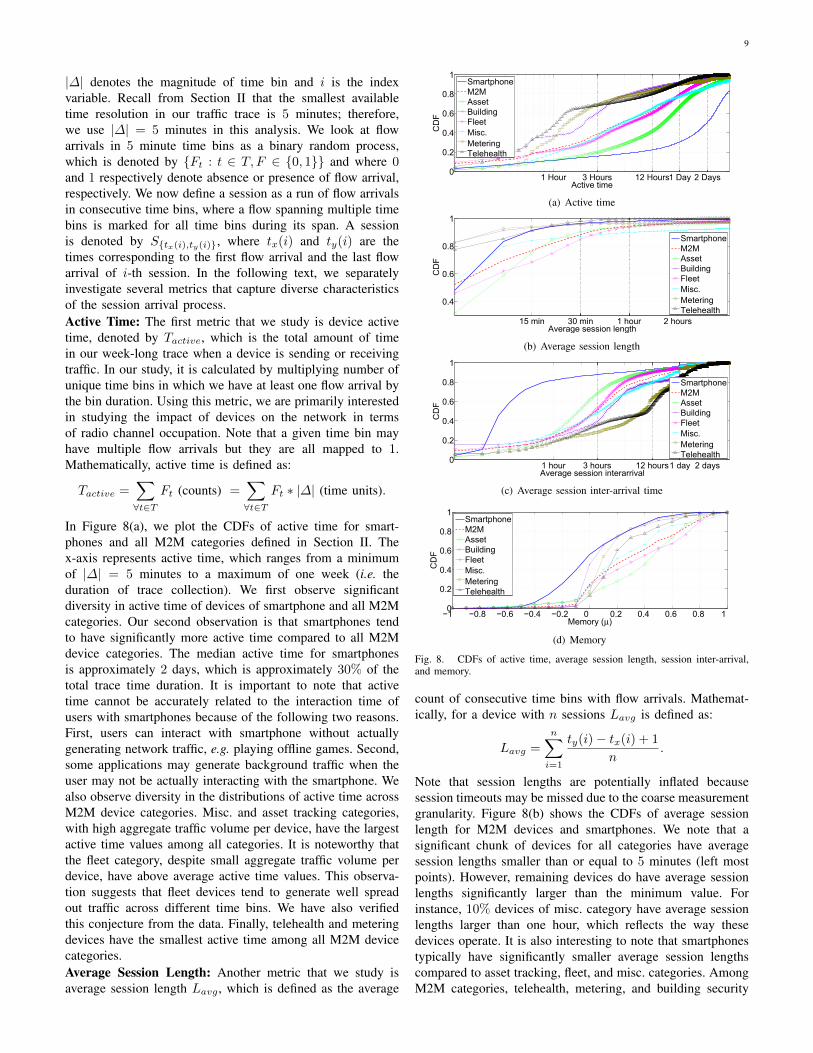
In Figure 8(a), we plot the CDFs of active time for smart-phones and all M2M categories defined in Section II. Thex-axis represents active time, which ranges from a minimumof |∆| = 5 minutes to a maximum of one week (i.e. theduration of trace collection). We first observe significantdiversity in active time of devices of smartphone and all M2Mcategories. Our second observation is that smartphones tendto have significantly more active time compared to all M2Mdevice categories. The median active time for smartphonesis approximately 2 days, which is approximately 30% of thetotal trace time duration. It is important to note that activetime cannot be accurately related to the interaction time ofusers with smartphones because of the following two reasons.First, users can interact with smartphone without actuallygenerating network traffic, e.g. playing offline games. Second,some applications may generate background traffic when theuser may not be actually interacting with the smartphone. Wealso observe diversity in the distributions of active time acrossM2M device categories. Misc. and asset tracking categories,with high aggregate traffic volume per device, have the largestactive time values among all categories. It is noteworthy thatthe fleet category, despite small aggregate traffic volume perdevice, have above average active time values. This observa-tion suggests that fleet devices tend to generate well spreadout traffic across different time bins. We have also verifiedthis conjecture from the data. Finally, telehealth and meteringdevices have the smallest active time among all M2M devicecategories.Average Session Length: Another metric that we study isaverage session length Lavg , which is defined as the average

1 Hour 3 Hours 12 Hours1 Day 2 Days0

0.2

0.4

0.6

0.8

1

Active time

CD

F


(a) Active time

15 min 30 min 1 hour 2 hours

0.4

0.6

0.8

1

Average session length

CD

F


(b) Average session length

1 hour 3 hours 12 hours1 day 2 days0

0.2

0.4

0.6

0.8

1

Average session interarrival

CD

F


(c) Average session inter-arrival time

−1 −0.8 −0.6 −0.4 −0.2 0 0.2 0.4 0.6 0.8 1 0

0.2

0.4

0.6

0.8

1

Memory (μ)

CD

F


(d) Memory

Fig. 8. CDFs of active time, average session length, session inter-arrival,and memory.

count of consecutive time bins with flow arrivals. Mathemat-ically, for a device with n sessions Lavg is defined as:

Lavg =

n∑i=1

ty(i)− tx(i) + 1

n.

Note that session lengths are potentially inflated becausesession timeouts may be missed due to the coarse measurementgranularity. Figure 8(b) shows the CDFs of average sessionlength for M2M devices and smartphones. We note that asignificant chunk of devices for all categories have averagesession lengths smaller than or equal to 5 minutes (left mostpoints). However, remaining devices do have average sessionlengths significantly larger than the minimum value. Forinstance, 10% devices of misc. category have average sessionlengths larger than one hour, which reflects the way thesedevices operate. It is also interesting to note that smartphonestypically have significantly smaller average session lengthscompared to asset tracking, fleet, and misc. categories. AmongM2M categories, telehealth, metering, and building security

10

have the smallest average session lengths.Average Session Inter-arrival: We also study the averagesession inter-arrival metric, which is defined as the averageof inter-arrival times between consecutive sessions. Using theearlier notion, we can mathematically define average sessioninter-arrival Tavg as follows:

Tavg =

n−1∑i=1

tx(i+ 1)− ty(i)n− 1

.

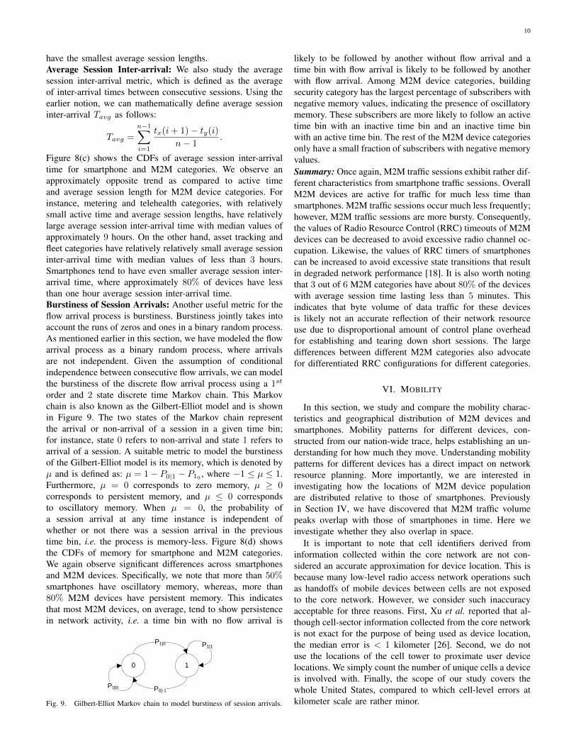
Figure 8(c) shows the CDFs of average session inter-arrivaltime for smartphone and M2M categories. We observe anapproximately opposite trend as compared to active timeand average session length for M2M device categories. Forinstance, metering and telehealth categories, with relativelysmall active time and average session lengths, have relativelylarge average session inter-arrival time with median values ofapproximately 9 hours. On the other hand, asset tracking andfleet categories have relatively relatively small average sessioninter-arrival time with median values of less than 3 hours.Smartphones tend to have even smaller average session inter-arrival time, where approximately 80% of devices have lessthan one hour average session inter-arrival time.Burstiness of Session Arrivals: Another useful metric for theflow arrival process is burstiness. Burstiness jointly takes intoaccount the runs of zeros and ones in a binary random process.As mentioned earlier in this section, we have modeled the flowarrival process as a binary random process, where arrivalsare not independent. Given the assumption of conditionalindependence between consecutive flow arrivals, we can modelthe burstiness of the discrete flow arrival process using a 1st

order and 2 state discrete time Markov chain. This Markovchain is also known as the Gilbert-Elliot model and is shownin Figure 9. The two states of the Markov chain representthe arrival or non-arrival of a session in a given time bin;for instance, state 0 refers to non-arrival and state 1 refers toarrival of a session. A suitable metric to model the burstinessof the Gilbert-Elliot model is its memory, which is denoted byµ and is defined as: µ = 1− P0|1 − P10 , where −1 ≤ µ ≤ 1.Furthermore, µ = 0 corresponds to zero memory, µ ≥ 0corresponds to persistent memory, and µ ≤ 0 correspondsto oscillatory memory. When µ = 0, the probability ofa session arrival at any time instance is independent ofwhether or not there was a session arrival in the previoustime bin, i.e. the process is memory-less. Figure 8(d) showsthe CDFs of memory for smartphone and M2M categories.We again observe significant differences across smartphonesand M2M devices. Specifically, we note that more than 50%smartphones have oscillatory memory, whereas, more than80% M2M devices have persistent memory. This indicatesthat most M2M devices, on average, tend to show persistencein network activity, i.e. a time bin with no flow arrival is

… -1 0-2 2 n1-n

P1|0

P0|-1

P2|1

P1|2

P3|2 Pn|n-1P-1|-2

P-2|-1

P0|-1

P-1|0

P-2|-3

Pn-1|nP2|3P-3|-2

P-n+1|-n

P-n|-n+1

…

0 1

P1|0

P0|-1

P1|1

P0|0

Fig. 9. Gilbert-Elliot Markov chain to model burstiness of session arrivals.

likely to be followed by another without flow arrival and atime bin with flow arrival is likely to be followed by anotherwith flow arrival. Among M2M device categories, buildingsecurity category has the largest percentage of subscribers withnegative memory values, indicating the presence of oscillatorymemory. These subscribers are more likely to follow an activetime bin with an inactive time bin and an inactive time binwith an active time bin. The rest of the M2M device categoriesonly have a small fraction of subscribers with negative memoryvalues.Summary: Once again, M2M traffic sessions exhibit rather dif-ferent characteristics from smartphone traffic sessions. OverallM2M devices are active for traffic for much less time thansmartphones. M2M traffic sessions occur much less frequently;however, M2M traffic sessions are more bursty. Consequently,the values of Radio Resource Control (RRC) timeouts of M2Mdevices can be decreased to avoid excessive radio channel oc-cupation. Likewise, the values of RRC timers of smartphonescan be increased to avoid excessive state transitions that resultin degraded network performance [18]. It is also worth notingthat 3 out of 6 M2M categories have about 80% of the deviceswith average session time lasting less than 5 minutes. Thisindicates that byte volume of data traffic for these devicesis likely not an accurate reflection of their network resourceuse due to disproportional amount of control plane overheadfor establishing and tearing down short sessions. The largedifferences between different M2M categories also advocatefor differentiated RRC configurations for different categories.

VI. MOBILITY

In this section, we study and compare the mobility charac-teristics and geographical distribution of M2M devices andsmartphones. Mobility patterns for different devices, con-structed from our nation-wide trace, helps establishing an un-derstanding for how much they move. Understanding mobilitypatterns for different devices has a direct impact on networkresource planning. More importantly, we are interested ininvestigating how the locations of M2M device populationare distributed relative to those of smartphones. Previouslyin Section IV, we have discovered that M2M traffic volumepeaks overlap with those of smartphones in time. Here weinvestigate whether they also overlap in space.

It is important to note that cell identifiers derived frominformation collected within the core network are not con-sidered an accurate approximation for device location. This isbecause many low-level radio access network operations suchas handoffs of mobile devices between cells are not exposedto the core network. However, we consider such inaccuracyacceptable for three reasons. First, Xu et al. reported that al-though cell-sector information collected from the core networkis not exact for the purpose of being used as device location,the median error is < 1 kilometer [26]. Second, we do notuse the locations of the cell tower to proximate user devicelocations. We simply count the number of unique cells a deviceis involved with. Finally, the scope of our study covers thewhole United States, compared to which cell-level errors atkilometer scale are rather minor.

11

1 10 100 0

0.2

0.4

0.6

0.8

1

Unique cell count

CD

F


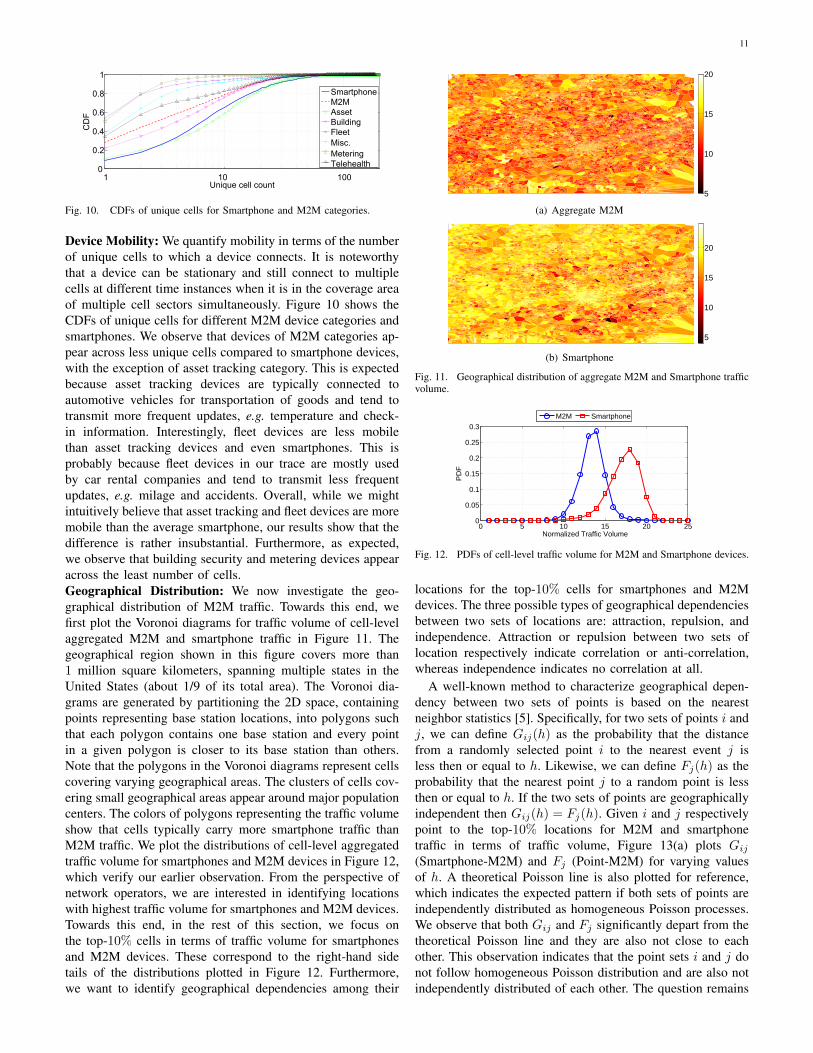
Fig. 10. CDFs of unique cells for Smartphone and M2M categories.

Device Mobility: We quantify mobility in terms of the numberof unique cells to which a device connects. It is noteworthythat a device can be stationary and still connect to multiplecells at different time instances when it is in the coverage areaof multiple cell sectors simultaneously. Figure 10 shows theCDFs of unique cells for different M2M device categories andsmartphones. We observe that devices of M2M categories ap-pear across less unique cells compared to smartphone devices,with the exception of asset tracking category. This is expectedbecause asset tracking devices are typically connected toautomotive vehicles for transportation of goods and tend totransmit more frequent updates, e.g. temperature and check-in information. Interestingly, fleet devices are less mobilethan asset tracking devices and even smartphones. This isprobably because fleet devices in our trace are mostly usedby car rental companies and tend to transmit less frequentupdates, e.g. milage and accidents. Overall, while we mightintuitively believe that asset tracking and fleet devices are moremobile than the average smartphone, our results show that thedifference is rather insubstantial. Furthermore, as expected,we observe that building security and metering devices appearacross the least number of cells.Geographical Distribution: We now investigate the geo-graphical distribution of M2M traffic. Towards this end, wefirst plot the Voronoi diagrams for traffic volume of cell-levelaggregated M2M and smartphone traffic in Figure 11. Thegeographical region shown in this figure covers more than1 million square kilometers, spanning multiple states in theUnited States (about 1/9 of its total area). The Voronoi dia-grams are generated by partitioning the 2D space, containingpoints representing base station locations, into polygons suchthat each polygon contains one base station and every pointin a given polygon is closer to its base station than others.Note that the polygons in the Voronoi diagrams represent cellscovering varying geographical areas. The clusters of cells cov-ering small geographical areas appear around major populationcenters. The colors of polygons representing the traffic volumeshow that cells typically carry more smartphone traffic thanM2M traffic. We plot the distributions of cell-level aggregatedtraffic volume for smartphones and M2M devices in Figure 12,which verify our earlier observation. From the perspective ofnetwork operators, we are interested in identifying locationswith highest traffic volume for smartphones and M2M devices.Towards this end, in the rest of this section, we focus onthe top-10% cells in terms of traffic volume for smartphonesand M2M devices. These correspond to the right-hand sidetails of the distributions plotted in Figure 12. Furthermore,we want to identify geographical dependencies among their

5

10

15

20

(a) Aggregate M2M

5

10

15

20

(b) Smartphone

Fig. 11. Geographical distribution of aggregate M2M and Smartphone trafficvolume.

0 5 10 15 20 250

0.05

0.1

0.15

0.2

0.25

0.3

Normalized Traffic Volume

PD

F

M2M Smartphone

Fig. 12. PDFs of cell-level traffic volume for M2M and Smartphone devices.

locations for the top-10% cells for smartphones and M2Mdevices. The three possible types of geographical dependenciesbetween two sets of locations are: attraction, repulsion, andindependence. Attraction or repulsion between two sets oflocation respectively indicate correlation or anti-correlation,whereas independence indicates no correlation at all.

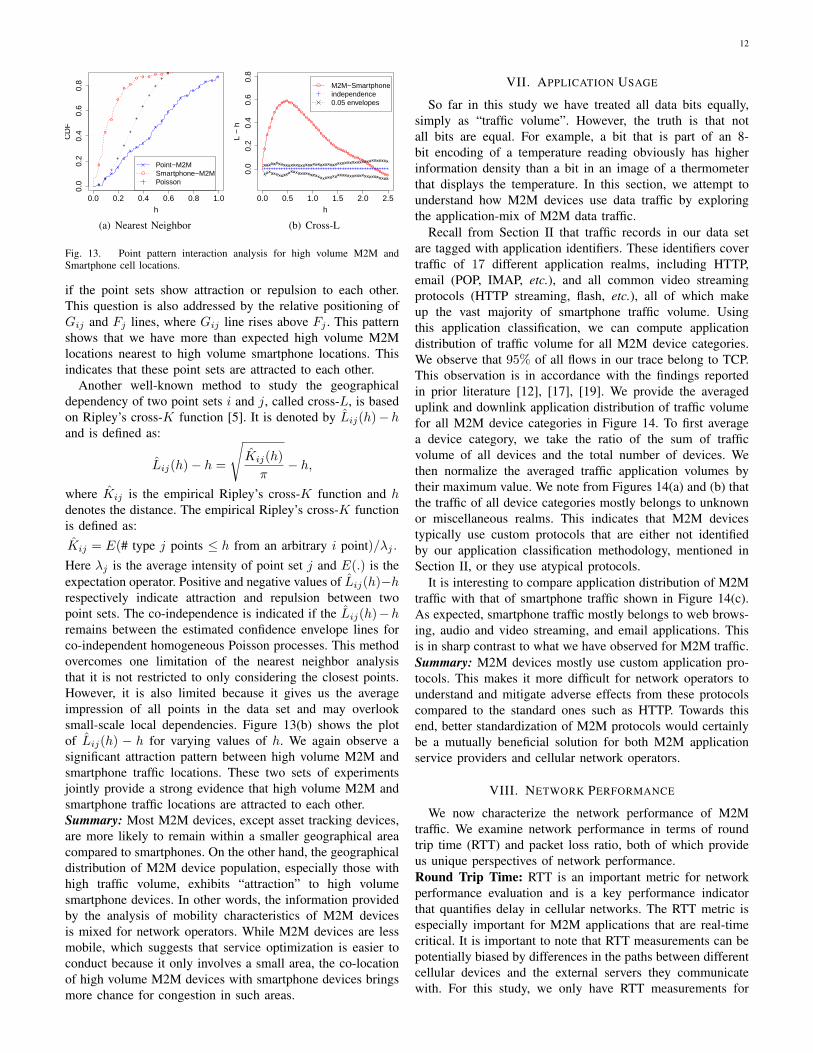
A well-known method to characterize geographical depen-dency between two sets of points is based on the nearestneighbor statistics [5]. Specifically, for two sets of points i andj, we can define Gij(h) as the probability that the distancefrom a randomly selected point i to the nearest event j isless then or equal to h. Likewise, we can define Fj(h) as theprobability that the nearest point j to a random point is lessthen or equal to h. If the two sets of points are geographicallyindependent then Gij(h) = Fj(h). Given i and j respectivelypoint to the top-10% locations for M2M and smartphonetraffic in terms of traffic volume, Figure 13(a) plots Gij(Smartphone-M2M) and Fj (Point-M2M) for varying valuesof h. A theoretical Poisson line is also plotted for reference,which indicates the expected pattern if both sets of points areindependently distributed as homogeneous Poisson processes.We observe that both Gij and Fj significantly depart from thetheoretical Poisson line and they are also not close to eachother. This observation indicates that the point sets i and j donot follow homogeneous Poisson distribution and are also notindependently distributed of each other. The question remains

12

x x

x x x

x

x x

x x

x x

x

x

x x

x

x x x

0.0 0.2 0.4 0.6 0.8 1.0

0.0

0.2

0.4

0.6

0.8

h

CD

F

o

o o

o

o

o o o o

o o o o

+

+ + + + + + + + + +

+

Point−M2MSmartphone−M2MPoisson

(a) Nearest Neighbor

o o o o o o o o

o o o o o o o o o o o o o o o o o o o o o o o o o o o o o o o o o o o o o o o o o o o

0.0 0.5 1.0 1.5 2.0 2.5

0.0

0.2

0.4

0.6

0.8

h

L −

h

x x x

x x x x x x x x x x x x x x x x x x x x x x x x x x x x

x x x x x x x x x x x x x x

x x x x x x

x x x x x x x x x

x x

x x x x x x x x x x x x x x x x x x x

x x x x x x x x x x x x x x x x x x x x x

+ + + + + + + + + + + + + + + + + + + + + + + + + + + + + + + + + + + + + + + + + + + + + + + + + + +

M2M−Smartphoneindependence0.05 envelopes

(b) Cross-L

Fig. 13. Point pattern interaction analysis for high volume M2M andSmartphone cell locations.

if the point sets show attraction or repulsion to each other.This question is also addressed by the relative positioning ofGij and Fj lines, where Gij line rises above Fj . This patternshows that we have more than expected high volume M2Mlocations nearest to high volume smartphone locations. Thisindicates that these point sets are attracted to each other.

Another well-known method to study the geographicaldependency of two point sets i and j, called cross-L, is basedon Ripley’s cross-K function [5]. It is denoted by L̂ij(h)− hand is defined as:

L̂ij(h)− h =

√K̂ij(h)

π− h,

where K̂ij is the empirical Ripley’s cross-K function and hdenotes the distance. The empirical Ripley’s cross-K functionis defined as:K̂ij = E(# type j points ≤ h from an arbitrary i point)/λj .Here λj is the average intensity of point set j and E(.) is theexpectation operator. Positive and negative values of L̂ij(h)−hrespectively indicate attraction and repulsion between twopoint sets. The co-independence is indicated if the L̂ij(h)−hremains between the estimated confidence envelope lines forco-independent homogeneous Poisson processes. This methodovercomes one limitation of the nearest neighbor analysisthat it is not restricted to only considering the closest points.However, it is also limited because it gives us the averageimpression of all points in the data set and may overlooksmall-scale local dependencies. Figure 13(b) shows the plotof L̂ij(h) − h for varying values of h. We again observe asignificant attraction pattern between high volume M2M andsmartphone traffic locations. These two sets of experimentsjointly provide a strong evidence that high volume M2M andsmartphone traffic locations are attracted to each other.Summary: Most M2M devices, except asset tracking devices,are more likely to remain within a smaller geographical areacompared to smartphones. On the other hand, the geographicaldistribution of M2M device population, especially those withhigh traffic volume, exhibits “attraction” to high volumesmartphone devices. In other words, the information providedby the analysis of mobility characteristics of M2M devicesis mixed for network operators. While M2M devices are lessmobile, which suggests that service optimization is easier toconduct because it only involves a small area, the co-locationof high volume M2M devices with smartphone devices bringsmore chance for congestion in such areas.

VII. APPLICATION USAGE

So far in this study we have treated all data bits equally,simply as “traffic volume”. However, the truth is that notall bits are equal. For example, a bit that is part of an 8-bit encoding of a temperature reading obviously has higherinformation density than a bit in an image of a thermometerthat displays the temperature. In this section, we attempt tounderstand how M2M devices use data traffic by exploringthe application-mix of M2M data traffic.

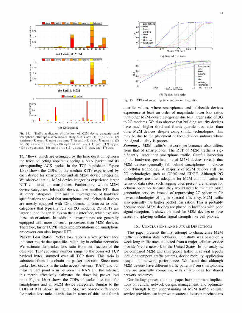
Recall from Section II that traffic records in our data setare tagged with application identifiers. These identifiers covertraffic of 17 different application realms, including HTTP,email (POP, IMAP, etc.), and all common video streamingprotocols (HTTP streaming, flash, etc.), all of which makeup the vast majority of smartphone traffic volume. Usingthis application classification, we can compute applicationdistribution of traffic volume for all M2M device categories.We observe that 95% of all flows in our trace belong to TCP.This observation is in accordance with the findings reportedin prior literature [12], [17], [19]. We provide the averageduplink and downlink application distribution of traffic volumefor all M2M device categories in Figure 14. To first averagea device category, we take the ratio of the sum of trafficvolume of all devices and the total number of devices. Wethen normalize the averaged traffic application volumes bytheir maximum value. We note from Figures 14(a) and (b) thatthe traffic of all device categories mostly belongs to unknownor miscellaneous realms. This indicates that M2M devicestypically use custom protocols that are either not identifiedby our application classification methodology, mentioned inSection II, or they use atypical protocols.

It is interesting to compare application distribution of M2Mtraffic with that of smartphone traffic shown in Figure 14(c).As expected, smartphone traffic mostly belongs to web brows-ing, audio and video streaming, and email applications. Thisis in sharp contrast to what we have observed for M2M traffic.Summary: M2M devices mostly use custom application pro-tocols. This makes it more difficult for network operators tounderstand and mitigate adverse effects from these protocolscompared to the standard ones such as HTTP. Towards thisend, better standardization of M2M protocols would certainlybe a mutually beneficial solution for both M2M applicationservice providers and cellular network operators.

VIII. NETWORK PERFORMANCE

We now characterize the network performance of M2Mtraffic. We examine network performance in terms of roundtrip time (RTT) and packet loss ratio, both of which provideus unique perspectives of network performance.Round Trip Time: RTT is an important metric for networkperformance evaluation and is a key performance indicatorthat quantifies delay in cellular networks. The RTT metric isespecially important for M2M applications that are real-timecritical. It is important to note that RTT measurements can bepotentially biased by differences in the paths between differentcellular devices and the external servers they communicatewith. For this study, we only have RTT measurements for

13

Dow

nlin

k tr

affic

vol

ume

1 2 3 4 5 6 7 8 9 10 11 12 13 14 15 16 170

0.25

0.5

0.75

1Asset Building Fleet Misc. Metering Telehealth

(a) Downlink M2M

Upl

ink

traf

fic v

olum

e

1 2 3 4 5 6 7 8 9 10 11 12 13 14 15 16 170

0.25

0.5

0.75

1Asset Building Fleet Misc. Metering Telehealth

(b) Uplink M2M

1 2 3 4 5 6 7 8 9 10 11 12 13 14 15 16 170

0.25

0.5

0.75

1

Tra

ffic

volu

me

Downlink Uplink

(c) Smartphone

Fig. 14. Traffic application distributions of M2M device categories andsmartphone. The application indices along x-axis are: (1) appstore, (2)jabber, (3) mms, (4) navigation, (5) email, (6) ftp, (7) gaming, (8)im, (9) miscellaneous, (10) optimization, (11) p2p, (12) apps,(13) streaming, (14) unknown, (15) voip, (16) vpn, and (17) web.

TCP flows, which are estimated by the time duration betweenthe trace collecting apparatus seeing a SYN packet and itscorresponding ACK packet in the TCP handshake. Figure15(a) shows the CDFs of the median RTTs experienced byeach device for smartphones and all M2M device categories.We observe that all M2M device categories experience largerRTT compared to smartphones. Furthermore, within M2Mdevice categories, telehealth devices have smaller RTT thanall other categories. Our manual investigation of hardwarespecifications showed that smartphones and telehealth devicesare mostly equipped with 3G modems, in contrast to othercategories that typically rely on 2G modems. 2G RTTs arelarger due to longer delays on the air interface, which explainsthese observations. In addition, smartphones are generallyequipped with more powerful processors than M2M devices.Therefore, faster TCP/IP stack implementations on smartphoneprocessors can also impact RTT.Packet Loss Ratio: Packet loss ratio is a key performanceindicator metric that quantifies reliability in cellular networks.We estimate the packet loss ratio from the fraction of theobserved TCP sequence number range to the observed TCPpayload bytes, summed over all TCP flows. This ratio issubtracted from 1 to obtain the packet loss ratio. Since mostpacket loss occurs in the radio access network (RAN) and ourmeasurement point is in between the RAN and the Internet,this metric effectively estimates the downlink packet lossratio. Figure 15(b) shows the CDFs of packet loss ratio forsmartphones and all M2M device categories. Similar to theCDFs of RTT shown in Figure 15(a), we observe differencesfor packet loss ratio distribution in terms of third and fourth

0.25 0.5 0.75 1 20

0.2

0.4

0.6

0.8

1

CD

F

Median RTT (sec)


(a) Round trip time

0.025 0.05 0.075 0.1 0.2 0.3 0.4 0.50

0.2

0.4

0.6

0.8

1

Packet Loss Ratio

CD

F


(b) Packet loss ratio

Fig. 15. CDFs of round trip time and packet loss ratio.

quartile values, where smartphones and telehealth devicesexperience at least an order of magnitude lower loss ratiosthan other M2M device categories due to a larger ratio of 3Gto 2G modems. We also observe that building security deviceshave much higher third and fourth quartile loss ratios thanother M2M devices, despite using similar technologies. Thismay be due to the placement of these devices indoors wherethe signal quality is poorer.Summary: M2M traffic’s network performance also differsfrom that of smartphones. The RTT of M2M traffic is sig-nificantly larger than smartphone traffic. Careful inspectionof the hardware specifications of M2M devices reveals thatM2M devices generally fall behind smartphones in choiceof cellular technology. A majority of M2M devices still use2G technologies such as GPRS and EDGE. Although 2Gtechnologies are often adequate for M2M communication interms of data rates, such lagging does present a challenge forcellular operators because they would need to maintain oldergeneration services, instead of repurposing 2G spectrum fornewer technologies of higher spectral efficiency. M2M trafficalso generally has higher packet loss ratios. This is probablybecause some M2M devices are placed in locations with poorsignal reception. It shows the need for M2M devices to havescreens displaying cellular signal strength like cell phones.

IX. CONCLUSIONS AND FUTURE DIRECTIONS

This paper presents the first attempt to characterize M2Mtraffic in cellular data networks. Our study was based on aweek long traffic trace collected from a major cellular serviceprovider’s core network in the United States. In our analysis,we compared M2M and smartphone traffic in several aspectsincluding temporal traffic patterns, device mobility, applicationusage, and network performance. We found that althoughM2M devices have different traffic patterns from smartphones,they are generally competing with smartphones for sharednetwork resources.

Our findings presented in this paper have important implica-tions on cellular network design, management, and optimiza-tion. Through better understanding of M2M traffic, cellularservice providers can improve resource allocation mechanisms

14

and develop better billing strategies for different categories ofM2M devices. Towards this end, Software Defined Networking(SDN) can be used for device- or subscriber-aware dynamicand flexible resource allocation and management [15]. SDNcan also help to isolate or slice cellular network resourcesvia virtualization to avoid contention between smartphoneand M2M traffic. Note that this isolation or slicing can befine-grained for different M2M device categories, or evendifferent M2M applications. Moreover, delay tolerant andnon-mission critical M2M traffic can be relayed over whitespaces. The aforementioned network design and managementtechniques can impact the dynamics of M2M traffic and in turnmay require introduction of novel pricing models by networkoperators.

REFERENCES

[1] AT&T specialty vertical devices. http://www.rfwel.com/support/hw-support/ATT SpecialtyVerticalDevices.pdf.

[2] 3G machine-to-machine (M2M) communications: Cellular 3G, WiMAX,and municipal Wi-Fi for M2M applications. Technical report, ABIre-search, 2007.

[3] The global wireless M2M market. Technical report, Berg Insight,December 2010.

[4] Cisco visual networking index: Global mobile data traffic forecastupdate, 2011-2016. White Paper, 2012.

[5] R. S. Bivand, E. J. Pebesma, and V. Gomez-Rubio. Applied SpatialData Analysis with R. Springer, 2008.

[6] CalAmp. LMU-2600 GPRS fleet tracking unit. http://www.calamp.com/pdf/LMU-2600.pdf.

[7] P. Chaovalit, A. Gangopadhyay, G. Karabatis, and Z. Chen. Discretewavelet transform-based time series analysis and mining. ACM Com-puting Surveys, 43(2), 2011.

[8] R. Coifman and M. Wickerhauser. Entropy-based algorithms for bestbasis selection. IEEE Transactions on Information Theory, 38(2 Part2):713–718, 1992.

[9] X. Dimitropoulos, P. Hurley, A. Kind, and M. P. Stoecklin. On the 95-percentile billing method. In International Conference on Passive andActive Network Measurement (PAM), 2009.

[10] J. Erman, A. Gerber, M. T. Hajiaghayi, D. Pei, and O. Spatscheck.Network-aware forward caching. In WWW, 2009.

[11] Z. M. Fadlullah, M. M. Fouda, N. K. A. Takeuchi, N. Iwasaki, andY. Nozaki. Toward intelligent machine-to-machine communications insmart grid. IEEE Communications Magazine, 49(4):60–65, 2011.

[12] A. Gerber, J. Pang, O. Spatscheck, and S. Venkataraman. Speed testingwithout speed tests: Estimating achievable download speed from passivemeasurements. In ACM IMC, 2010.

[13] N. Grira, M. Crucianu, and N. Boujemaa. Unsupervised and semi-supervised clustering: A brief survey. Report of the MUSCLE EuropeanNetwork of Excellence (FP6), 2004.

[14] L. K. Law, S. V. Krishnamurthy, and M. Faloutsos. Capacity of hybridcellular-ad hoc data networks. In INFOCOM, 2008.

[15] L. E. Li, Z. M. Mao, and J. Rexford. CellSDN: Software-defined cellularnetworks. Technical report, Princeton University Computer ScienceTechnical Report, 2012.

[16] Z. Moczar and S. Molnar. Comparative traffic analysis study ofpopular applications. In International Conference on Energy-awareCommunications, 2011.

[17] U. Paul, A. P. Subramanian, M. M. Buddhikot, and S. R. Das. Un-derstanding traffic dynamics in cellular data networks. In INFOCOM,2011.

[18] F. Qian, Z. Wang, A. Gerber, Z. M. Mao, S. Sen, and O. Spatscheck.Characterizing radio resource allocation for 3G networks. In ACM IMC,2010.

[19] M. Z. Shafiq, L. Ji, A. X. Liu, J. Pang, and J. Wang. Characterizinggeospatial dynamics of application usage in a 3G cellular data network.In IEEE INFOCOM, 2012.

[20] M. Z. Shafiq, L. Ji, A. X. Liu, and J. Wang. Characterizing and modelingInternet traffic dynamics of cellular devices. In ACM SIGMETRICS,2011.

[21] L. Song and J. Shen, editors. Evolved Cellular Network Planning andOptimization for UMTS and LTE. CRC, 2010.

[22] P. Stoica and R. L. Moses. Introduction to Spectral Analysis. PrenticeHall, 1997.

[23] P. Traynor, M. Lin, M. Ongtang, V. Rao, T. Jaeger, P. McDaniel, andT. L. Porta. On cellular botnets: measuring the impact of maliciousdevices on a cellular network core. In ACM CCS, 2009.

[24] Trilliant. CellReader digital cellular meters. http://www.trilliantinc.com/products/cellreader/.

[25] I. T. Union. World telecommunication/ICT indicators database 2011.http://www.itu.int/ITU-D/ict/ publications/world/world.html, 2011.

[26] Q. Xu, A. Gerber, Z. M. Mao, and J. Pang. AccuLoc: Practicallocalization of peformance measurement in 3G networks. In ACMMobiSys, 2011.

M. Zubair Shafiq received his B.E. degree in Elec-trical Engineering from National University of Sci-ences and Technology, Islamabad, Pakistan in 2008.He is currently a Ph.D. candidate in the Departmentof Computer Science and Engineering at MichiganState University. He was co-recipient of the IEEEICNP 2012 Best Paper Award. He also received the2012 Fitch-Beach Outstanding Graduate ResearchAward by College of Engineering, Michigan StateUniversity. His research interests are in big dataanalytics and performance modeling.

Lusheng Ji is a Principal Member of TechnicalStaff - Research at the AT&T Shannon Laboratory,Florham Park, New Jersey. He received his Ph.D. inComputer Science from the University of Maryland,College Park in 2001. His research interests includewireless networking, mobile computing, wirelesssensor networks, and networking security. He is aSenior Member of the IEEE.

Alex X. Liu received his Ph.D. degree in computerscience from the University of Texas at Austin in2006. He received the IEEE & IFIP William C.Carter Award in 2004 and an NSF CAREER awardin 2009. He received the Withrow DistinguishedScholar Award in 2011 at Michigan State University.He is an Associate Editor of IEEE/ACM Transac-tions on Networking. He received Best Paper Awardsfrom ICNP-2012, SRDS-2012, and LISA-2010. Hisresearch interests focus on networking and security.

Jeffrey Pang is a researcher at AT&T Labs -Research. He received his Ph.D. in Computer Sci-ence from Carnegie Mellon University in 2009. Hecurrently builds systems to measure and optimizecellular networks. His research interests include net-working, mobile systems, distributed systems, andprivacy.

Jia Wang received her Ph.D. in Computer Sci-ence from Cornell University in January 2001. Shejoined AT&T Labs - Research since then and isnow a Principal Technical Staff Member in theNetwork Measurement and Engineering ResearchDepartment. Her research interests focus on networkmeasurement and management, network security,performance analysis and troubleshooting, IPTV, so-cial networks, and cellular networks.

Documents

Large Scale Measurement and Characterization of Cellular ...alexliu/publications/M2M/Main_ToN_MSU.pdf · Large Scale Measurement and Characterization of ... To answer this question,