Embed Size (px)
Citation preview
Large scale dynamics of the Persistent Turning Walker
model of fish behavior
Pierre Degond and Sebastien MotschInstitute of Mathematics of Toulouse
UMR 5219 (CNRS-UPS-INSA-UT1-UT2),Universite Paul Sabatier,118, route de Narbonne,
31062 Toulouse cedex, [email protected], [email protected]
Abstract
This paper considers a new model of individual displacement, based on fishmotion, the so-called Persistent Turning Walker (PTW) model, which involves anOrnstein-Uhlenbeck process on the curvature of the particle trajectory. The goalis to show that its large time and space scale dynamics is of diffusive type, andto provide an analytic expression of the diffusion coefficient. Two methods areinvestigated. In the first one, we compute the large time asymptotics of the varianceof the individual stochastic trajectories. The second method is based on a diffusionapproximation of the kinetic formulation of these stochastic trajectories. The kineticmodel is a Fokker-Planck type equation posed in an extended phase-space involvingthe curvature among the kinetic variables. We show that both methods lead to thesame value of the diffusion constant. We present some numerical simulations toillustrate the theoretical results.
Key words. Individual based model ; Fish behavior ; Persistent Turning Walker model; Ornstein-Uhlenbeck process ; Kinetic Fokker-Planck equation ; Asymptotic analysis ;Diffusion approximation
AMS subject classification: 35Q80, 35K99, 60J70, 82C31, 82C41, 82C70, 82C80,92D50
Acknowledgements. The authors wish to thank Guy Theraulaz and Jacques Gautraisof the ’Centre de Recherches sur la Cognition Animale’ in Toulouse, for introducing themto the model and for stimulating discussions.
1 Introduction
This paper considers a new model of individual displacement, the so-called ’PersistentTurning Walker’ (PTW) model, which has recently been introduced to describe fish be-
1
havior [28]. The fish evolves with a velocity of constant magnitude and its trajectoryis subject to random turns (i.e. random changes of curvature) on the one hand and tocurvature relaxation to zero on the other hand. The random changes of curvature canbe interpreted as a way for the fish to explore its surroundings while relaxation to zerocurvature just expresses that the fish cannot sustain too strongly curved trajectories andthat, when the curvature becomes too large, the fish tries to return to a straight linetrajectory. The combination of these two antagonist behaviors gives rise to an Ornstein-Uhlenbeck process on the curvature. The curvature is the time derivative of the director ofthe velocity, while the velocity itself is the time derivative of position. The PTW processcollects all these considerations into a system of stochastic differential equations.
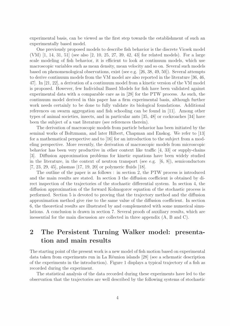
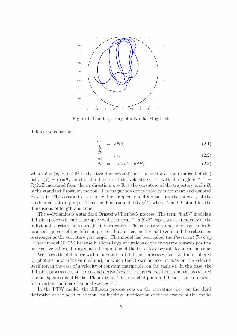
This model is, to the knowledge of the authors, original, and has appeared for the firsttime in the works by Gautrais, Theraulaz, and coworkers [28]. It has been deduced from astatistical analysis of data issued from experiments run in La Reunion islands during years2001 and 2002. The studied species is a pelagic fish named Kuhlia Mugil. Its typical sizeranges between 20 and 25 cm. The first experiments have been made with a single fishin a basin of 4 meters diameter during two minutes. A video records the positions of thefish every 12-th of a second (see figure 1 below). Then, after a filtering of the oscillatoryswimming motion of the fish, the trajectories have been fitted to model trajectories.
The more classical process consisting of a fish moving along straight lines and un-dergoing random changes of its velocity direction according to a Poisson process (like aphoton in a diffusive medium) has been discarded. Indeed, statistical tests have shown[28] that the befitting of the actual trajectory of a fish to a broken line interpolatingthe trajectory at random points did not lead to a satisfactory agreement. On the otherhand, a better fitting was obtained when the trajectory was interpolated by a sequenceof circular arcs connected to each other with a continuous tangent. It was then observedthat the curvatures of these circles followed a process which can be viewed as a realizationof an Ornstein-Uhlenbeck process on the curvature. This was the starting point of thePTW process. The experiments and the data analysis are reported in full detail in [28].
Then, the experiments were reproduced with 2, 5, 15 and 30 fish in the basin. Theanalyses of the interactions among the fish population are still in progress. In the presentwork, we will concentrate on the modeling of a single fish behaviour based on the PTWmodel and we will postpone the modeling of interacting individuals to future time, whenthe analysis of the data will be available. However, we will have in mind that the modelsissued from the analysis of a single fish behaviour must be easily expanded to model largegroups of interacting fish.
The present paper considers the large time and space scale dynamics of a two-dimensionalparticle subject to this PTW process. It rigorously shows (in the mathematical sense)that, at large scales, the dynamics of the particle can be described by a diffusion processand it provides a formula for the diffusion coefficient. To prove this result, two methodsare considered.
In the first method, the stochastic differential system itself is considered and thevariance of the position is shown to behave, at large times, like a linear function of time.The diffusion coefficient is identified as the slope of this linear function. Because thecurvature and the velocity angle can be explicitly computed, an explicit formula for thediffusion coefficient, involving some special functions, can be obtained.
2
The second method considers the forward Kolmogorov equation of the stochastic pro-cess. This equation gives the evolution of the probability distribution function of theparticle in the extended phase space (position, velocity angle, curvature) as a functionof time. It is a Fokker-Planck type equation. The passage from the microscopic to themacroscopic scales relies on a rescaling of the Kolmogorov equation. This rescaling de-pends on a small parameter ε ≪ 1, which describes the ratio of the typical microscopicto macroscopic space units. After this rescaling, the problem has the typical form of thediffusion approximation of a kinetic problem (see references below). The goal is then tostudy the behaviour of the solution as ε → 0. It is shown that the solution convergesto some ’thermodynamical equilibrium’ which is a Gaussian distribution of the curvatureand a uniform distribution of the velocity angle. The equilibrium depends parametricallyon the density which satisfies a spatial diffusion equation.
Finally, the connection between the two methods is made by showing that the diffu-sion tensor in the second approach can be represented by a formula involving the solutionof the stochastic differential equation of the first approach. Additionally, this represen-tation leads to explicit computations which show that the two formulas for the diffusioncoefficient actually coincide. This seemingly innocuous result is actually quite powerful.Indeed, the diffusion approximation method leads to a non-explicit expression of the dif-fusion coefficient, involving the moments of a particular solution of a stationary equationinvolving the leading order operator of the Fokker-Planck equation. That this non-explicitformula is equivalent to the explicit formula given by the stochastic trajectory methodis by far not obvious. In this respect, the stochastic trajectory method is more powerfulthan the diffusion approximation approach, because it directly leads to the most simpleexpression of the diffusion constant.
A third route could have been taken and has been dismissed. This third method wouldactually use the stochastic differential equation itself to perform the diffusion approxima-tion in the forward Kolmogorov equation. We have preferred to use partial differentialequation techniques. One reason for this choice is that these techniques can be moreeasily extended to more complex situations. One typical example of these more complexsituations are the nonlinear systems which are obtained when interactions between indi-vidual are included. The inclusion of interactions between individuals within the PTWmodel is actually work in progress.
From the biological viewpoint, one should not restrict the content of the paper to thesole expression of the diffusion coefficient. Indeed, once interactions between individualswill be included in the PTW model, it is not clear at all that the explicit computationswhich led to this expression will still be tractable. In the absence of an explicit solutionof the stochastic differential system, there is little grasp to get information about thelarge scale behaviour of the system. By contrast, the diffusion approximation approachgives a systematic tool to study the large scale behavior of such systems, in all kinds ofsituations, be they linear or nonlinear. By its flexibility and its versatility, the diffusionapproximation approach is the method of choice to study these problems.
The ultimate goal of this work programme is the establishment of a macroscopic modelfor large groups of fish. However, such a model must be based on a reliable model forthe individual displacements, since interactions lead to an alteration of the individualbehaviour in the absence of interaction. Therefore, the present work, which has a solid
3
experimental basis, can be viewed as the first step towards the establishment of such anexperimentally based model.
One previously proposed models to describe fish behavior is the discrete Vicsek model(VM) [1, 14, 31, 51] (see also [2, 10, 25, 27, 39, 42, 43] for related models). For a largescale modeling of fish behavior, it is efficient to look at continuum models, which usemacroscopic variables such as mean density, mean velocity and so on. Several such modelsbased on phenomenological observations, exist (see e.g. [26, 38, 49, 50]). Several attemptsto derive continuum models from the VM model are also reported in the literature [36, 46,47]. In [21, 22], a derivation of a continuum model from a kinetic version of the VM modelis proposed. However, few Individual Based Models for fish have been validated againstexperimental data with a comparable care as in [28] for the PTW process. As such, thecontinuum model derived in this paper has a firm experimental basis, although furtherwork needs certainly to be done to fully validate its biological foundations. Additionalreferences on swarm aggregation and fish schooling can be found in [11]. Among othertypes of animal societies, insects, and in particular ants [35, 48] or cockroaches [34] havebeen the subject of a vast literature (see references therein).
The derivation of macroscopic models from particle behavior has been initiated by theseminal works of Boltzmann, and later Hilbert, Chapman and Enskog. We refer to [13]for a mathematical perspective and to [16] for an introduction to the subject from a mod-eling perspective. More recently, the derivation of macroscopic models from microscopicbehavior has been very productive in other context like traffic [4, 33] or supply-chains[3]. Diffusion approximation problems for kinetic equations have been widely studiedin the literature, in the context of neutron transport (see e.g. [6, 8]), semiconductors[7, 23, 29, 45], plasmas [17, 19, 20] or polymeric fluids [18].
The outline of the paper is as follows : in section 2, the PTW process is introducedand the main results are stated. In section 3 the diffusion coefficient is obtained by di-rect inspection of the trajectories of the stochastic differential system. In section 4, thediffusion approximation of the forward Kolmogorov equation of the stochastic process isperformed. Section 5 is devoted to proving that the trajectory method and the diffusionapproximation method give rise to the same value of the diffusion coefficient. In section6, the theoretical results are illustrated by and complemented with some numerical simu-lations. A conclusion is drawn in section 7. Several proofs of auxiliary results, which areinessential for the main discussion are collected in three appendix (A, B and C).
2 The Persistent Turning Walker model: presenta-
tion and main results
The starting point of the present work is a new model of fish motion based on experimentaldata taken from experiments run in La Reunion islands [28] (see a schematic descriptionof the experiments in the introduction). Figure 1 displays a typical trajectory of a fish asrecorded during the experiment.
The statistical analysis of the data recorded during these experiments have led to theobservation that the trajectories are well described by the following systems of stochastic
4
−2 −1.5 −1 −0.5 0 0.5 1 1.5 2
−1.5
−1
−0.5
0
0.5
1
1.5
Figure 1: One trajectory of a Kuhlia Mugil fish
differential equations:
d~x
dt= c~τ(θ), (2.1)
dθ
dt= cκ, (2.2)
dκ = −aκ dt+ b dBt, (2.3)
where ~x = (x1, x2) ∈ R2 is the (two-dimensional) position vector of the (centroid of the)
fish, ~τ(θ) = (cos θ , sin θ) is the director of the velocity vector with the angle θ ∈ Π =R/2πZ measured from the x1 direction, κ ∈ R is the curvature of the trajectory and dBt
is the standard Brownian motion. The magnitude of the velocity is constant and denotedby c > 0. The constant a is a relaxation frequency and b quantifies the intensity of therandom curvature jumps. b has the dimension of 1/(L
√T ) where L and T stand for the
dimensions of length and time.The κ-dynamics is a standard Ornstein-Uhlenbeck process. The term “b dBt” models a
diffusion process in curvature space while the term “−aK dt” expresses the tendency of theindividual to return to a straight line trajectory. The curvature cannot increase endlesslyas a consequence of the diffusion process, but rather, must relax to zero and the relaxationis stronger as the curvature gets larger. This model has been called the Persistent TurningWalker model (PTW) because it allows large excursions of the curvature towards positiveor negative values, during which the spinning of the trajectory persists for a certain time.
We stress the difference with more standard diffusion processes (such as those sufferedby photons in a diffusive medium), in which the Brownian motion acts on the velocityitself (or, in the case of a velocity of constant magnitude, on the angle θ). In this case, thediffusion process acts on the second derivative of the particle positions, and the associatedkinetic equation is of Fokker-Planck type. This model of photon diffusion is also relevantfor a certain number of animal species [41].
In the PTW model, the diffusion process acts on the curvature, i.e. on the thirdderivative of the position vector. An intuitive justification of the relevance of this model
5
for animal behaviour is by considering the non-differentiability of the Brownian motion.Because of this feature, the photon diffusion process involves infinite second derivatives ofthe position, i.e. infinite forces. However, an animal body can only exert finite forces andthe muscles act only in such a way that the velocity angle undergoes smooth variations.The PTW model precisely presents this feature of having smooth second order derivatives,i.e. smooth forces.
Our goal in the present work is to study the large-scale dynamics of the stochasticdifferential system (2.1)-(2.3). This is best done in scaled variables, where the dimension-less parameters of the model are highlighted. We use t0 = a−1 as time unit, x0 = ca−1
as space unit, and κ0 = x−10 as curvature unit, and we introduce the dimensionless time,
space and curvature as t′ = t/t0, x′ = x/x0 and κ′ = κ/κ0. For simplicity, we omit the
primes. In scaled variables, the PTW model is written:
d~x
dt= ~τ(θ), (2.4)
dθ
dt= κ, (2.5)
dκ = −κ dt+√2αdBt, (2.6)
where the only dimensionless parameter left is α such that
α2 =b2c2
2a3, (2.7)
The meaning of α2 is the following: b/√a is the amplitude of a curvature change during
a relaxation time a−1, while c/a is obviously the distance travelled by the particle duringthis time. The product of these two quantities is dimensionless and is equal to
√2α. It
quantifies the strength of the curvature jumps relative to the other phenomena.The individual dynamics can be translated in terms of a probability distribution
f(t, ~x, θ, κ) d~x dθ dκ of finding particles at times t with position in small neighborhoodsd~x dθ dκ of position ~x, velocity angle θ and curvature κ. The link between the individ-ual dynamics and the evolution of the probability distribution f is given by the forwardKolmogorov equation :
∂tf + ~τ · ∇~xf + κ∂θf − ∂κ(κf)− α2∂κ2f = 0. (2.8)
This equation is an exact transcription of the individual dynamics, where the initialvalue f0 at time t = 0 is given by the probability distribution of the initial conditions ofthe stochastic differential system (2.4)-(2.6). For more detailed considerations about theforward Kolmogorov equation and its link with stochastic differential systems, we referthe reader to [40, 5].
In order to capture the macroscopic dynamics, two possible routes can be taken, usingeither the stochastic differential system (2.4)-(2.6) or the partial differential equation(2.8). In this work, we follow both routes and verify that they lead to the same large-scale behaviour. The advantage of working directly on the stochastic system is that itis simpler and it leads to explicit formulas. However, as soon as the system gets morecomplicated, and in particular nonlinear, explicit solutions can no longer be found and
6
this methodology can hardly be pursued. On the other hand, the PDE approach, which,in the present case is more complicated, is also more systematic and more general. Inparticular, it is generally usable in the more complex nonlinear cases (see e.g. [21, 22]).A particular important complex situation is the case of many interacting fish. In futurework, we plan to extend the PTW model to populations of interacting fish and to use thePDE approach to extract the large-scale dynamics of the system.
From the analysis of the individual trajectories, explicit exact expressions for κ andθ in terms of stochastic integrals can be found. Unfortunately, there is no such explicitresult for the position ~x(t), but we can calculate the first two moments of the probabilitydistribution of ~x(t) explicitly, using the expressions of κ and θ. We show that the mean ofthe position vector stays at the origin: E{~x(t)} = (0, 0) (where E denotes the expectationover all sources of randomness, in the initial data and in the stochastic process) and thatthe variance grows asymptotically linearly in time. More exactly, we prove:
Theorem 2.1 Under assumptions on the initial conditions that will be specified later on(see (3.1)-(3.4)), the solution of system (2.4)-(2.6) satisfies:
Var{~x(t)} t→+∞∼ 2D t, with D =
∫ ∞
0
exp(
−α2(−1 + s+ e−s))
ds. (2.9)
The notation Var is for the variance over all sources of randomness. The asymptoticlinear growth of the variance (2.9) suggests that the dynamics of the system is of diffusivetype at large times with diffusion coefficient D. We can find an expression of D in termsof special functions. Indeed, we have
Proposition 2.2 The following expression holds true:
D =( e
α2
)α2
γ(α2, α2), (2.10)
where γ(z, u) is the incomplete gamma function:
γ(z, u) =
∫ u
0
e−t tz−1 dt. (2.11)
D has the following series representation:
D = eα2
∞∑
n=0
(−1)nα2n
n! (n+ α2). (2.12)
It is a decreasing function of α which has the following asymptotic behavior:
D ∼ 1
α2as α → 0, D ∼
√
π
2
1
αas α → ∞. (2.13)
7
To investigate the large scale dynamics of the solution of the kinetic equation (2.8)(the existence of which can be easily proved, see proposition 4.2), we need to rescale thevariables to the macroscopic scale. Indeed, in eq. (2.8), all the coefficients are supposedto be of order unity. This means that the time and space scales of the experiment are ofthe same order as the typical time and length scales involved in the dynamics, such as,the relaxation time or the inverse of the typical random curvature excursions. Of course,in most experiments, this is not true, since the duration of the experiment and the sizeof the experimental region are large compared with the time and length scales involvedin the dynamics.
To translate this observation, we change the space unit x0 to a new space space unitx′0 = x0/ε, where ε ≪ 1 is a small parameter. This induces a change of variables x′ = εx.
We make a similar operation on the time unit t′0 = t0/η, t′ = ηt with η ≪ 1. Now, the
question of linking η to ε is a subtle one and is largely determined by the nature of theasymptotic regime which is achieved by the system. In the present case, we expect thatthe asymptotic regime will be of diffusive nature, in view of theorem 2.1 and so, we willinvestigate the so-called ’diffusion approximation’ which involves a quadratic relationshipbetween η and ε: η = ε2.
For this reason, we introduce the diffusive rescaling:
t′ = ε2t ; ~x′ = ε~x, (2.14)
and we make the following change of variable in the distribution f :
f ε(t′, ~x′, θ, κ) =1
ε2f
(
t′
ε2,~x′
ε, θ, κ
)
.
The scaling of the magnitude of the distribution function is unnecessary, since the prob-lem is linear. However, it is chosen in order to preserve the total number of particles.Introducing (2.14) into (2.8) leads to the following problem for f ε:
ε∂tfε + ~τ · ∇~xf
ε +1
ε[κ∂θf
ε − ∂κ(κfε)− α2∂κ2f ε ] = 0 (2.15)
In order to analyze the large-scale dynamics of (2.15), we need to investigate the limitε → 0. We show that f ε converges to an equilibrium distribution function (i.e. a functionwhich cancels the O(ε−1) term of (2.15)) f 0 which depends parametrically on the particledensity n0(x, t) and n0 evolves according to a diffusion equation. More precisely, we prove:
Theorem 2.3 Under hypothesis 4.1 on the initial data to be precised below, the solutionf ε of (2.15) converge weakly in a Banach space also to be specified below, (see (4.21)) X:
f ε ε→0⇀ n0 M(κ)
2πin X weak star, (2.16)
where M is a Gaussian distribution of the curvature with zero mean and variance α2 (see4.4) and n0 = n0(x, t) is the solution of the system:
∂tn0 +∇~x · J0 = 0, (2.17)
J0 = −D∇~xn0, (2.18)
where the initial datum n00 and the diffusion tensor D will be defined later on (see (4.31)
and (4.28) respectively).
8
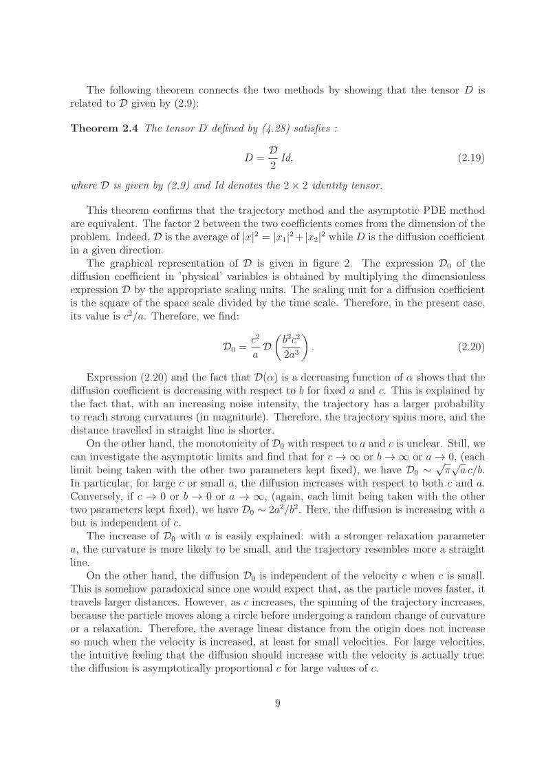
The following theorem connects the two methods by showing that the tensor D isrelated to D given by (2.9):
Theorem 2.4 The tensor D defined by (4.28) satisfies :
D =D2Id, (2.19)
where D is given by (2.9) and Id denotes the 2× 2 identity tensor.
This theorem confirms that the trajectory method and the asymptotic PDE methodare equivalent. The factor 2 between the two coefficients comes from the dimension of theproblem. Indeed, D is the average of |x|2 = |x1|2+ |x2|2 while D is the diffusion coefficientin a given direction.
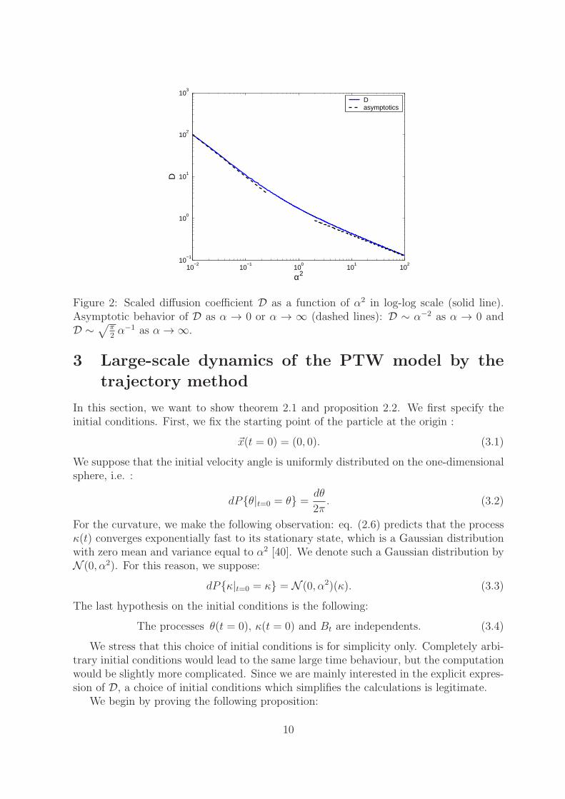
The graphical representation of D is given in figure 2. The expression D0 of thediffusion coefficient in ’physical’ variables is obtained by multiplying the dimensionlessexpression D by the appropriate scaling units. The scaling unit for a diffusion coefficientis the square of the space scale divided by the time scale. Therefore, in the present case,its value is c2/a. Therefore, we find:
D0 =c2
aD(
b2c2
2a3
)
. (2.20)
Expression (2.20) and the fact that D(α) is a decreasing function of α shows that thediffusion coefficient is decreasing with respect to b for fixed a and c. This is explained bythe fact that, with an increasing noise intensity, the trajectory has a larger probabilityto reach strong curvatures (in magnitude). Therefore, the trajectory spins more, and thedistance travelled in straight line is shorter.
On the other hand, the monotonicity of D0 with respect to a and c is unclear. Still, wecan investigate the asymptotic limits and find that for c → ∞ or b → ∞ or a → 0, (eachlimit being taken with the other two parameters kept fixed), we have D0 ∼ √
π√a c/b.
In particular, for large c or small a, the diffusion increases with respect to both c and a.Conversely, if c → 0 or b → 0 or a → ∞, (again, each limit being taken with the othertwo parameters kept fixed), we have D0 ∼ 2a2/b2. Here, the diffusion is increasing with abut is independent of c.
The increase of D0 with a is easily explained: with a stronger relaxation parametera, the curvature is more likely to be small, and the trajectory resembles more a straightline.
On the other hand, the diffusion D0 is independent of the velocity c when c is small.This is somehow paradoxical since one would expect that, as the particle moves faster, ittravels larger distances. However, as c increases, the spinning of the trajectory increases,because the particle moves along a circle before undergoing a random change of curvatureor a relaxation. Therefore, the average linear distance from the origin does not increaseso much when the velocity is increased, at least for small velocities. For large velocities,the intuitive feeling that the diffusion should increase with the velocity is actually true:the diffusion is asymptotically proportional c for large values of c.
9
10−2
10−1
100
101
102
10−1
100
101
102
103
α2
D
Dasymptotics
Figure 2: Scaled diffusion coefficient D as a function of α2 in log-log scale (solid line).Asymptotic behavior of D as α → 0 or α → ∞ (dashed lines): D ∼ α−2 as α → 0 andD ∼√π
2α−1 as α → ∞.
3 Large-scale dynamics of the PTW model by the
trajectory method
In this section, we want to show theorem 2.1 and proposition 2.2. We first specify theinitial conditions. First, we fix the starting point of the particle at the origin :
~x(t = 0) = (0, 0). (3.1)
We suppose that the initial velocity angle is uniformly distributed on the one-dimensionalsphere, i.e. :
dP{θ|t=0 = θ} =dθ
2π. (3.2)
For the curvature, we make the following observation: eq. (2.6) predicts that the processκ(t) converges exponentially fast to its stationary state, which is a Gaussian distributionwith zero mean and variance equal to α2 [40]. We denote such a Gaussian distribution byN (0, α2). For this reason, we suppose:
dP{κ|t=0 = κ} = N (0, α2)(κ). (3.3)
The last hypothesis on the initial conditions is the following:
The processes θ(t = 0), κ(t = 0) and Bt are independents. (3.4)
We stress that this choice of initial conditions is for simplicity only. Completely arbi-trary initial conditions would lead to the same large time behaviour, but the computationwould be slightly more complicated. Since we are mainly interested in the explicit expres-sion of D, a choice of initial conditions which simplifies the calculations is legitimate.
We begin by proving the following proposition:
10
Proposition 3.1 The solution of the stochastic differential equation (2.4)-(2.6) with ini-tial condition given by (3.1)-(3.4) satisfies :
E{~x(t)} = (0, 0) , ∀ t ≥ 0, (3.5)
Var{~x(t)} = 2
∫ t
s=0
(t− s) exp(
−α2(
−1 + s+ e−s))
ds. (3.6)
To prove this proposition, we first establish explicit formulae for the solutions of (2.5)and (2.6). The proof is deferred to appendix A.
Lemma 3.2 The solution of the stochastic differential system (2.5), (2.6) with initialconditions (3.2)-(3.4) is given by:
θ(t) = θ0 + κ0 − κ(t) +√2αBt, (3.7)
κ(t) = e−tκ0 +√2αe−t
∫ t
0
es dBs. (3.8)
Additionally,
θ(t) = θ0 +Kt0, (3.9)
where Kt0 is a Gaussian random variable independent of θ0 with zero mean and variance
β2t given by :
β2t = Var{Kt
0} = 2α2(−1 + t+ e−t). (3.10)
Proof of proposition 3.1: Using Lemma 3.2, we can compute the first two momentsof ~x(t). Let us start with the computation of the mean. If we write ~x(t) = (x1(t) , x2(t)),we have :
x1(t) =
∫ t
0
cos θ(s) ds , x2(t) =
∫ t
0
sin θ(s) ds,
and, computing the mean :
E{x1(t)} = E
{∫ t
0
cos θ(s) ds
}
=
∫ t
0
E {cos θ(s)} ds.
Now, we can develop θ(s) using (3.9):
E {cos θ(s)} = E {cos(θ0 +Ks0)} = E {cos θ0 cosKs
0 − sin θ0 sinKs0} .
By the independence of θ0 and Ks0 we finally have:
E {cos θ(s)} = E{cos θ0}E{cosKs0} − E{sin θ0}E{sinKs
0} = 0,
since the expectations of cos θ0 and sin θ0 over the uniform probability distribution on θ0are zero. Finally, we have E{x1(t)} = 0, and similarly for x2. This proves (3.5).
11
Now for the variance of ~x(t), we write:
Var{~x(t)} = E{x21(t) + x2
2(t)} = 2E{x21(t)}. (3.11)
by the isotropy of the problem. Then,
E{x21(t)} = E
{
(∫ t
0
cos θ(s) ds
)2}
=
∫ t
0
∫ t
0
E{cos θ(s) cos θ(u)} dsdu
= 2
∫ t
0
du
∫ u
0
ds E{cos θ(s) cos θ(u)}.
Since u ≥ s, we can write θ(u) as follows :
θ(u) = θ0 +
∫ s
0
κ(z) dz +
∫ u
s
κ(z) dz = θ0 +Ks0 +Ku
s ,
where Ks0 and Ku
s are Gaussian random variables independent of θ0 with zero mean andvariances β2
s and β2u−s respectively, thanks to (3.10). Then, using standard identities for
trigonometric functions, we get
E{cos θ(s) cos θ(u)} = E{cos(θ0 +Ks0) cos(θ0 +Ks
0 +Kus )}
=1
2(cos(2θ0 + 2Ks
0 +Kus ) + cos(−Ku
s )).
But since θ0 is independent of Ks0 and Ku
s we have E{cos(2θ0+2Ks0 +Ku
s )} = 0 since themean of a cos(θ0 +C) over the uniform distribution of θ0 is zero whatever the value of C.Then :
E{cos θ(s) cos θ(u)} =1
2E{cos (−Ku
s )}
=1
2
∫
R
cos(y)1√
2πβu−s
e− y2
2β2u−s dy
=1
2e−
1
2β2
u−s .
Indeed, an elementary computation shows that for any Gaussian random variable Z withzero mean and variance σ2, one has
E{cos(Z)} = exp(−σ2/2). (3.12)
Thus,
E{x1(t)2} =
∫ t
u=0
∫ u
s=0
exp(
−α2(
−1 + |u− s|+ e−|u−s|))
dsdu.
Using the change of unknowns w = u− s and y = u and inverting the order of integrationwe find :
E{x1(t)2} =
∫ t
w=0
(t− w) exp(
−α2(
−1 + w + e−w))
dw.
12
Using (3.11), we finally find (3.6), which ends the proof of the proposition.
In order to prove 2.1, we investigate the behavior of the variance Var{~x(t)} (given by(3.6)) when t → +∞.
End of proof of Theorem 2.1: We write, thanks to (3.6):
Var{~x(t)} − 2Dt = −2
∫ t
s=0
se−α2(−1+s+e−s) ds− 2
∫ ∞
s=t
te−α2(−1+s+es) ds.
We have to show that the difference is bounded independently of t. For the first term, wehave:
∣
∣
∣
∣
∫ t
s=0
se−α2(−1+s+e−s) ds
∣
∣
∣
∣
≤∫ t
0
eα2
se−α2s ds,
and integrating by parts, we find :
∣
∣
∣
∣
∫ t
s=0
se−α2(−1+s+es) ds
∣
∣
∣
∣
≤ eα2
α2
[
−te−α2t − e−α2t
α2+
1
α2
]
≤ C1.
For the second term, we have:
∣
∣
∣
∣
∫ ∞
s=t
te−α2(−1+s+es) ds
∣
∣
∣
∣
≤ t
∫ ∞
t
eα2
e−α2s ds ≤ teα2 e−tα2
α2≤ C2.
This proves that the difference is Var{~x(t)} − 2Dt is bounded independently of t andcompletes the proof.
We now prove Proposition 2.2 which gives an explicit approximation of the diffusioncoefficient. This approximation is useful for practical simulations.
Proof of Proposition 2.2: The change of variables t = α2e−s in the integral (2.9)leads to (2.10). The series representation (2.12) follows from a similar series represen-tation of the incomplete gamma function (see e.g. formula (8.354) of [30]). The seriesrepresentation can also be found by expanding the exponential in the integral (2.11) inpower series (this point is left to the reader). That D is a decreasing function of α followsfrom (2.9) and the fact that the function g(s) = −1 + s + exp(−s) is non-negative fors ≥ 0. The behavior of D for α → 0 (first formula (2.13)) is obtained by keeping onlythe zero-th order term in the series expansion (2.12). From (2.9), the behaviour of D forα → ∞ is controled by the behaviour of g(s) near s = 0. Since g(s) ∼ s2/2, we findD ∼
∫∞
0exp(−α2s2/2) ds, which leads to the second formula (2.13), and ends the proof.
13
4 Large-scale dynamics of the PTW model through
the diffusion approximation of the associated ki-
netic equation
4.1 Formal asymptotics
In this section, for the reader’s convenience, we give a formal proof of theorem 2.3. Wewrite (2.15) as follows:
ε∂tfε + ~τ · ∇~xf
ε +1
εAf ε = 0 (4.1)
where we define the operator A acting on functions u(θ, κ) as follows:
Au = κ∂θu− ∂κ(κu)− α2∂κ2u. (4.2)
The formal investigation of the limit ε → 0 usually starts by considering the Hilbertexpansion (see e.g. [16] for the general theory or [20] for an application in the context ofFokker-Planck equations):
f ε = f 0 + εf 1 +O(ε2), (4.3)
with fk being independent of ε and inserting it into (4.1). Then, collecting all the theterms of comparable orders with respect to ε, we are led to a sequence of equations. Thefirst one, corresponding to the leading O(ε−1) term is Af 0 = 0, which means that f 0 liesin the kernel of A. In section 4.3, we show that the kernel of A is composed of functionsof the form f 0(t, ~x, θ, κ) = n0(t, ~x)M(κ)/(2π) where M(κ) is a normalized Gaussian withzero mean and variance α2:
M(κ) =1√2πα2
e−κ2
2α2 , (4.4)
and n0(t, ~x) is a function still to be determined.In order to determine n0, we first integrate (4.1) with respect to (θ, κ) ∈ Π × R and
use that∫
Audθ dκ = 0. Defining the density nε(t, ~x) and the flux Jε(t, ~x) by
nε(t, ~x) =
∫
θ,κ
f ε dκ dθ, Jε(t, ~x) =
∫
θ,κ
f ε
ε~τ(θ) dκdθ, (4.5)
we find:
∂tnε +∇~x · Jε = 0. (4.6)
We note that this continuity equation is valid for all values of ε. Then, letting ε → 0, weformally have nε → n0. If we prove that J0 given by (2.18) is the limit of Jε, as ε → 0,then, we can pass to the limit in (4.6) and find (2.17).
System (2.17) and (2.18) is a diffusion system, which completely determines n0(t, ~x),given its initial datum n0
0(~x). Here, for simplicity, we assume that the initial datum for(4.1) is of the form f ε(0, ~x, θ, κ) = n0(~x)M(κ)/(2π) and the resulting initial condition forn0 is therefore n0
0 = n0 (in this formal convergence proof, we admit the functions and theconvergences are as smooth as required).
14
So, the only points left in the proof are the existence of a limit for Jε and the validityof (2.18) for J0. Note that the existence of a limit is not obvious because of the factor εat the denominator of the integral (4.5) defining Jε. To prove that the limit exists, weuse the Hilbert expansion (4.3) again and compute f 1. Since A is linear, collecting theterms of order O(ε0) leads to:
−Af 1 =M(κ)
2π~τ · ∇~xn
0 . (4.7)
Again using the linearity of A and the fact that it operates only with respect to the (θ, κ)variables, we can write the solution of (4.7) as f 1 = −~χ · ∇~xn
0, where ~χ = (χ1, χ2) is asolution of the problem
A~χ =M(κ)
2π~τ . (4.8)
This equation must be understood componentwise (i.e χ1 is associated with τ1 = cos θand χ2 with τ2 = sin θ). Since the right-hand side of (4.8) has zero average with respectto (θ, κ), proposition 4.5 below shows that it has a unique solution, up to an element ofthe kernel of A. We can single out a unique solution by requesting that ~χ has zero averagewith respect to (θ, κ) as well. Then, all solutions f 1 to (4.7) can be written as
f 1 = −~χ · ∇~xn0 + n1(t, ~x)
M(κ)
2π, (4.9)
where the second term of (4.9) is an arbitrary element of the kernel of A. We shall seethat the determination of n1 is unnecessary.
Now, inserting the Hilbert expansion (4.3) into the integral (4.5) defining Jε, we find:
Jε(t, ~x) =1
ε
∫
θ,κ
f 0 ~τ(θ) dκdθ +
∫
θ,κ
f 1 ~τ(θ) dκdθ +O(ε)
= 0 +
∫
θ,κ
f 1 ~τ(θ) dκdθ +O(ε), (4.10)
because f 0 is independent of θ and∫
~τ(θ) dθ = 0. Therefore, Jε has a limit when ε → 0and this limit is given by
J0(t, ~x) =
∫
θ,κ
f 1 ~τ(θ) dκdθ. (4.11)
To compute J0 we insert expression (4.9) into (4.11) and find
J0(t, ~x) =
∫
θ,κ
(−~χ · ∇~xn0 + n1M
2π)~τ(θ) dκdθ. (4.12)
The second term vanishes and the first one can be written
J0(t, ~x) = −(∫
θ,κ
~τ ⊗ ~χ dθ dκ
)
∇~xn0, (4.13)
15
which is nothing but formula (2.18) with the diffusivity tensor D given by (4.28).This shows the formal convergence of the solution of the Fokker-Planck equation (2.15)
to that of the diffusion system (2.17), (2.18).Now, to make this proof rigorous, we need to justify all the formal convergences. In
the framework of the Hilbert expansion, this requires to work out the regularity of thevarious terms of the expansion. This is doable and actually leads to stronger convergencesthan the one we are going to prove, but this is a bit technical (see e.g. [20]).
What we are going to do instead is proving a convergence result in a weaker topologywithout using the Hilbert expansion technique. The method is close to the so-calledmoment method, which consists in integrating the equation against suitable test functions.This convergence proof is developed in section 4.3, but before that, we state an existenceresult for the original Fokker-Planck equation (4.1).
4.2 Functional setting and existence result
We define the differential operator D acting on smooth functions f(κ) by :
Df = ∂κ(κf) + α2∂κ2f. (4.14)
We state some properties of D, the proofs of which are easy and left to the reader. Werecall that M(κ) denotes the normalized Gaussian with zero mean and variance α2 (4.4).
Proposition 4.1 Let f and g be smooth functions decreasing at infinity. The followingidentities hold true:
Df = α2 ∂
∂κ
(
M∂
∂κ
f
M
)
, (4.15)
∫
R
Df gdκ
M= −α2
∫
R
M ∂κ
(
f
M
)
∂κ
( g
M
)
dκ =
∫
R
f Dgdκ
M, (4.16)
∫
R
Df fdκ
M= −α2
∫
R
M
∣
∣
∣
∣
∂κ
(
f
M
)∣
∣
∣
∣
2
dκ ≤ 0, (4.17)
Df = 0 ⇔ ∃c ∈ R, f = cM. (4.18)
The first identity translates the fact that M is the stationary measure of the Ornstein-Uhlenbeck process. The second one that D is formally self-adjoint with respect to themeasure dκ/M . The third one shows thatD is dissipative. The same inequality holds withany non-decreasing function η(f), indeed,
∫
D(f) η(f)M−1 dκ ≤ 0. If η is the logarithmfunction, the corresponding quantity would be the relative entropy dissipation of f withrespect to M . Entropy plays an important role in kinetic theory (see [13] for a review).Finally, the last quantity states that the kernel of D is one-dimensional and spanned byM .
Proposition 4.1 shows that the natural L2 norm associated with this operator has aweight M−1 and that the natural H1 semi-norm is given by the right-hand side of (4.17).
16
This motivates the introduction of the following functional spaces, endowed with theirnaturally associated Hilbert structures and norms:
H = {u : Πθ × Rκ → R /
∫
θ,κ
|u(θ, κ)|2 dθdκM
< +∞}, (4.19)
V =
{
u ∈ H /
∫
Π,R
M∣
∣
∣∂κ
( u
M
)∣
∣
∣
2
dκdθ < +∞}
, (4.20)
L2M = L2(R2
~x, H), X = L2([0, T ]× R2~x, V ). (4.21)
Identifying H with its dual, with have a Hilbertian triple V ⊂ H ⊂ V ′, where V ′ is thedual of V and all injections are continuous. They are not compact because V does notbring any regularity with respect to θ.
The existence proof follows closely the existence proof of [15] (see appendix A of thisreference) and for this reason, is omitted (see also [20]). The proof relies on an existencetheorem due to J. L. Lions [37].
Proposition 4.2 Let ε > 0. We assume that f0 belongs to L2M defined by (4.21). Then
there exists a unique solution f ε to (2.15) with initial datum f 0 in the class of functionsY defined by :
Y ={
f ∈ X / ∂tf + ε−1~τ · ∇~xf + ε−2κ∂θf ∈ X ′}
.
Moreover, we have the inequality for any T > 0:
||f ε(T )||2L2
M+
α2
ε2
∫ T
0
∫
~x,θ,κ
M
∣
∣
∣
∣
∂κ
(
f ε
M
)∣
∣
∣
∣
2
dκ dθ d~x dt = ||f ε(0)||2L2
M. (4.22)
Estimate (4.22) is obtained via a Green and a trace formula for functions belongingto Y which can be deduced from the one proved in [15].
4.3 Rigorous asymptotics
We first study operator A given by (4.2), i.e. Af = κ∂θf−Df and state some propertieswhich will be proved in appendix B. We view A as an unbounded operator on the Hilbertspace H with domain D(A) given by:
D(A) = {u(θ, κ) ∈ V /Au ∈ H} .
Lemma 4.3 Operator A is maximal monotone. Moreover its kernel (or Null-space) isgiven by:
Ker(A) = {cM , c ∈ R}, (4.23)
with M defined by (4.4).
Lemma 4.4 The adjoint A∗ of A in H is given by A∗f = −κ∂θf −Df . It is a Maximalmonotone operator with domain D(A∗) = D(A) and Ker(A∗) = Ker(A).
17
Proposition 4.5 Let g ∈ H. Then, there exists u ∈ D(A) such that
Au = g, (4.24)
if and only if g satisfies the following solvability condition:∫
θ,κ
g(θ, κ) dθdκ = 0. (4.25)
Moreover, the solution u is unique up to a constant times M . A unique solution can besingled out by prescribing the condition
∫
θ,κ
u(θ, κ) dθdκ = 0. (4.26)
The same lemma applies to the equation A∗u = g.
As an application of this lemma, let ~χ be the solution of :
A~χ = ~τ(θ)M
2π, (4.27)
with ~τ(θ) = (cos θ , sin θ). Since τ has zero average over θ and κ, ~χ is well-defined andunique thanks to Proposition 4.5. Then, we define the tensor D by:
D =
∫
θ,κ
~τ(θ)⊗ ~χ dθdκ. (4.28)
Note that, since∫
θ,κ~τ(θ)M(κ) dθdκ = 0, it would not change the value of D to add any
element of Ker(A) to ~χ.
Lemma 4.6 Let R denote the reflection operator u(θ, κ) → Ru(θ, κ) = u(θ,−κ). Then,~χ∗ = R~χ is the unique solution (satisfying (4.26)) of
A∗~χ∗ = ~τ(θ)M
2π, (4.29)
and we have
D =
∫
θ,κ
~τ(θ)⊗ ~χ∗ dθdκ. (4.30)
Proof. Obviously, D commutes with R: DR = RD while κ∂θ anticommutes with R:κ∂θ(Ru) = −R(κ∂θu). Therefore, RA = A∗R. Since the right-hand side of (4.27) isinvariant by R, applying R to both sides of (4.27) leads to (4.29). Then, the change ofvariables κ′ = −κ in the integral at the right-hand side of (4.30) shows that it is equal toD.
To study the limit ε → 0, we make the following hypothesis on the initial conditions.
18
Hypothesis 4.1 We suppose that the initial condition f ε0 is uniformly bounded in L2
M
and converges weakly in L2M to f 0
0 as ε → 0.
We can now prove theorem 2.3. The initial datum for the diffusion system (2.17, (2.18)will be shown to be:
n0t=0 = n0
0 =
∫
θ,κ
f 00 (~x, θ, κ) dκdθ. (4.31)
Proof. of theorem 2.3: By hypothesis 4.1 inequality (4.22) implies :
||f ε(T )||2L2
M+
α2
ε2
∫ T
0
∫
~x,θ,κ
M
∣
∣
∣
∣
∂κ
(
f ε
M
)∣
∣
∣
∣
2
dκ dθ d~x dt ≤ C , (4.32)
with C independent of ε. So (f ε)ε is a bounded sequence in L∞(0, T, L2M ) and satisfies
∫ T
0
∫
~x,θ,κ
M
∣
∣
∣
∣
∂κ
(
f ε
M
)∣
∣
∣
∣
2
dκ dθ d~x dt ≤ Cε2 , (4.33)
for any time interval T (by the diagonal process, we will eventually be able to take anincreasing sequence of times T tending to infinity, so that the result will be valid on thewhole interval t ∈ (0,∞)). Therefore, there exists f 0 ∈ L∞(0, T, L2
M ) and a subsequence,still denoted by f ε, satisfying :
f ε ε→0⇀ f 0 in L∞(0, T, L2
M ) weak star .
Furthermore, with (4.33), we deduce that f 0 = C(~x, θ, t)M(κ). Then, letting ε → 0 in(2.15), we get that Af 0 = 0 in the distributional sense. This implies that C(~x, θ, t) isindependent of θ and we can write
f 0(t, ~x, θ, κ) = n0(t, ~x)M(κ)
2π, (4.34)
the quantity n0(t, ~x) =∫
f 0(t, ~x, θ, κ) dθ dκ being the density associated with f 0.Our next task is to show that n0 satisfies the diffusion model (2.17), (2.18) with initial
condition (4.31). We first note that f ε is a week solution of (2.15) with initial conditionf ε0 in the following sense: f ε satisfies:
∫ T
0
∫
~x,θ,κ
f ε(−ε∂tϕ− ~τ · ∇~xϕ+1
εA∗(ϕ))
dκdθd~x
Mdt = ε
∫
~x,θ,κ
f ε0ϕt=0
dκdθd~x
M, (4.35)
for all test functions ϕ in the space C2c ([0, T ) × R
2~x × Πθ × Rκ) of twice continuously
differentiable functions with compact support in [0, T )×R2~x ×Πθ ×Rκ. Again, the trace
at t = 0 has a meaning, thanks to a trace formula for functions in Y which is proven in[15].
We recall the definition of the flux (4.5). We prove that Jε has a weak limit asε → 0. To this aim, in the weak formulation (4.35), we take as a test function ϕ =~φ(t, ~x) · ~χ∗(θ, κ) with ~χ∗ the auxiliary function defined as the solution to (4.29) and ~φ is
19
a smooth compactly supported vector test function of (~x, t). Although ϕ does not havea compact support, a standard truncation argument (which is omitted here) can be usedto bypass this restriction. This allows us to write:
∫ T
0
∫
~x,θ,κ
[f ε(−ε∂t − (~τ · ∇~x))(~φ · ~χ∗) +1
εf ε~τ
M
2π· ~φ] dκdθd~x
Mdt = ε
∫
~x,θ,κ
f ε0~φt=0 · ~χ
dκdθd~x
M.
Taking the limit ε → 0, we find :
limε→0
∫ T
0
∫
~x
Jε · ~φ d~xdt = 2π
∫ T
0
∫
~x,θ,κ
f 0(~τ · ∇~x)(~φ · ~χ∗)dκdθd~x
Mdt
=
∫ T
0
∫
~x
n0 ∇~x ·(
(∫
θ,κ
~χ∗ ⊗ ~τ dκdθ
)T
~φ
)
d~xdt,
where the exponent T denotes the transpose of a matrix. Using (4.30) and taking the limitε → 0 shows that Jε converges weakly (in the distributional sense) towards J0 satisfying
∫ T
0
∫
~x
J0 · ~φ d~xdt =
∫ T
0
∫
~x
n0 ∇~x ·(
(D)T ~φ)
d~xdt.
This last equation is the weak form of eq. (2.18).Finally, to prove (2.17), we apply the weak formulation (4.35) to a test function of the
form ϕ = φ(t, ~x)M(κ), where again, φ(x, t) is a scalar, smooth and compactly supportedtest function of (~x, t) in R
2 × [0, T ). This gives :
−∫ T
0
∫
~x,θ,κ
f ε ((ε∂t + (~τ · ∇~x))ϕ) dκdθd~xdt = ε
∫
~x,θ,κ
f ε0φt=0 dκdθd~x.
Dividing by ε and taking the limit ε → 0, we get :
−∫ T
0
∫
~x
(n0∂tϕ+ J0 · ∇~xφ) d~xdt =
∫
~x
n00φt=0 d~x,
where n00 is defined by (4.31). This last equation is exactly the weak formulation of
equation (2.17), with initial datum n00. This concludes the proof.
5 Equivalence of the two methods
In this section, we show that both methods lead to the same value of the diffusion coeffi-cient (theorem 2.4).
The first step is to show that we can approximate the solution of equation (4.24) bythe solution of the associated evolution equation. More precisely, in appendix C, we provethe following lemma :
20
Lemma 5.1 Let g in H satisfying (4.25) and u∞ in D(A) be the solution of (4.24)satisfying (4.26). Let u0 ∈ D(A) satisfying (4.26). Then, the solution u(t) of the evolutionproblem:
∂tu = −Au + g , ut=0 = u0, (5.1)
weakly converges to u∞ in H as t tends to ∞.
With this lemma we can explicitly calculate the tensor D and prove the theorem 2.4 :
Proof of theorem 2.4: Let ~χ(t) be the solution of
∂t~χ = −A~χ + ~τ(θ)M(κ)
2π, ~χ(t = 0) = 0. (5.2)
Thanks to Lemma 5.1, ~χ(t) weakly converges to ~χ in H when t → ∞. It follows that :∫
κ,θ
~χ(t)⊗ ~τ dκdθt→+∞−→
∫
κ,θ
~χ⊗ ~τ dκdθ. (5.3)
Let us consider the first component of ~χ(t), which we denote by u(t) and the integrals∫
κ,θu(t) cos θ dκdθ and
∫
κ,θu(t) sin θ dκdθ . Because u satisfies (5.2), it admits the follow-
ing representation (see the proof of lemma 5.1):
u(t) =
∫ t
0
Ts
(
cos θM(κ)
2π
)
ds,
where Tt is the semi-group generated by −A (see [44]). With this expression, we evaluatethe integral of u(t) against cos θ :
∫
κ,θ
u(t) cos θ dκdθ =
∫
κ,θ
∫ t
0
Ts
(
cos θM(κ)
2π
)
ds cos θ dκ dθ
=
∫ t
0
∫
κ,θ
cos θM(κ)
2πT ∗s (cos θ) dκ dθ ds,
where T ∗ is the adjoint operator of T in L2(θ, κ) generated by −A∗, where
A∗(f) = −κ∂θf + κ∂κf − α2∂κ2f.
Note that we are referring here to the adjoint in the standard L2 sense and not in theweighted space H. This is why A∗ does not coincide with A∗ defined in Lemma 4.4. Thesemi-group T ∗
t admits a probabilistic representation: for all regular functions f(θ, κ)
T ∗t (f)(θ, κ) = E{f(θ(t), κ(t))|θ0 = θ, κ0 = κ},
where (κ(t), θ(t)) is the solution of the stochastic differential equation (2.5), (2.6). Usingthis representation, we have :
∫
κ
M(κ)T ∗s (cos θ) dκ =
∫
κ
M(κ)E{cos θs|θ0 = θ, κ0 = κ} dκ
= E{cos θs|θ0 = θ, κ0 = Z},
21
where Z is a random variable independent of Bt with density M . Using lemma 3.2, wehave :
E{cos θs|θ0 = θ, κ0 = Z} = E{cos(θ + Ys)},with Ys a Gaussian random variable with zero mean and variance β2
s given by (3.10).Then:
E{cos(θ + Ys)} = E{cos θ cosYs − sin θ sinYs} cos θ E{cosYs},because the density of Ys is even and implies that E{sinYs} = 0. Finally using (3.12), wehave:
∫
κ
M(κ)T ∗s (cos θ) dκ = cos θ e−
β2s2 .
Then, the first integral is given by:
∫
κ,θ
u(t) cos θ dκ dθ =
∫ t
0
∫
θ
cos θ
2πcos θ e−
β2s2 dθ ds
∫ t
0
1
2e−
β2s2 ds.
We can proceed similarly to evaluate the integral of u(t) against sin(t). This gives:
∫
κ,θ
u(t) sin θ dκdθ =
∫ t
0
∫
θ
cos θ sin θ
2πE{cosYs} dθds = 0.
It remains to evaluate the integrals involving the second component of vector ~χ(t) whichwe denote by v(t). By the same method as for u(t), we get :
∫
κ,θ
v(t) cos θ dκ dθ = 0 and
∫
κ,θ
v(t) sin θ dκ dθ =
∫ t
0
1
2e−
β2s2 dt.
Collecting these formulae, we can write:
∫
κ,θ
~χ(t)⊗ ~τ dκdθ =D(t)
2Id,
with D(t) =∫ t
0e−α2(−1+u+e−u) du. Taking the limit t → +∞ and using equation (5.3),
shows that (2.19) holds true and completes the proof of the theorem.
6 Numerical simulation
We simulate individual trajectories satisfying equation (2.4)-(2.6) with initial conditionsgiven by (3.1)-(3.4). If we fix a time step ∆t, using (3.7), (3.8), we have :
{
κ(n+1)∆t = γκn∆t +G(n+1)
θ(n+1)∆t = θ0 + κ0 − κ(n+1)∆t +√2αB(n+1)∆t
with γ = e−∆t and G(n+1) a Gaussian random variable with zero mean and variance2α2
(
1− e−2∆t)
independent of κn∆t. With this formula, we can simulate recursively theprocess (κn∆t, θn∆t)n exactly (in the sense that it has the same law as the exact solution).
22
To generate the Brownian motion, we just compute the increments B(n+1)∆t −Bn∆t sincethey are Gaussian and independent of Bn∆t. On the other hand, these increments arenot independent of G(n+1). Fortunately, we can compute the covariance matrix of theGaussian vector (G(n+1), B(n+1)∆t − Bn∆t) :
(
G(n+1)
B(n+1)∆t − Bn∆t
)
∼ N (0, C)
whereN (0, C) is a two-dimensional Gaussian vector with zero mean and covariance matrixC given by:
C =
[
2α2(
1− e−2∆t) √
2α(1− e−∆t)√2α(1− e−∆t) ∆t
]
.
Knowing this covariance matrix, we can simulate the Gaussian vector (G(n+1), B(n+1)∆t −Bn∆t) using the Cholesky method : we generate (X1, X2) a vector of two independentnormal law, and take
√C(X1, X2)
T as realization of the Gaussian vector.Now for the position ~x, since we do not have any explicit expression, we use a discrete
approximation scheme of order O((∆t)2). For example, the first component x1 of ~x isapproximated by:
x1((n+ 1)∆t) = x1(n∆t) +
∫ (n+1)∆t
n∆t
cos θ(s) ds
≈ x1(n∆t) +∆t
2(cos θ(n∆t) + cos θ((n+ 1)∆t)).
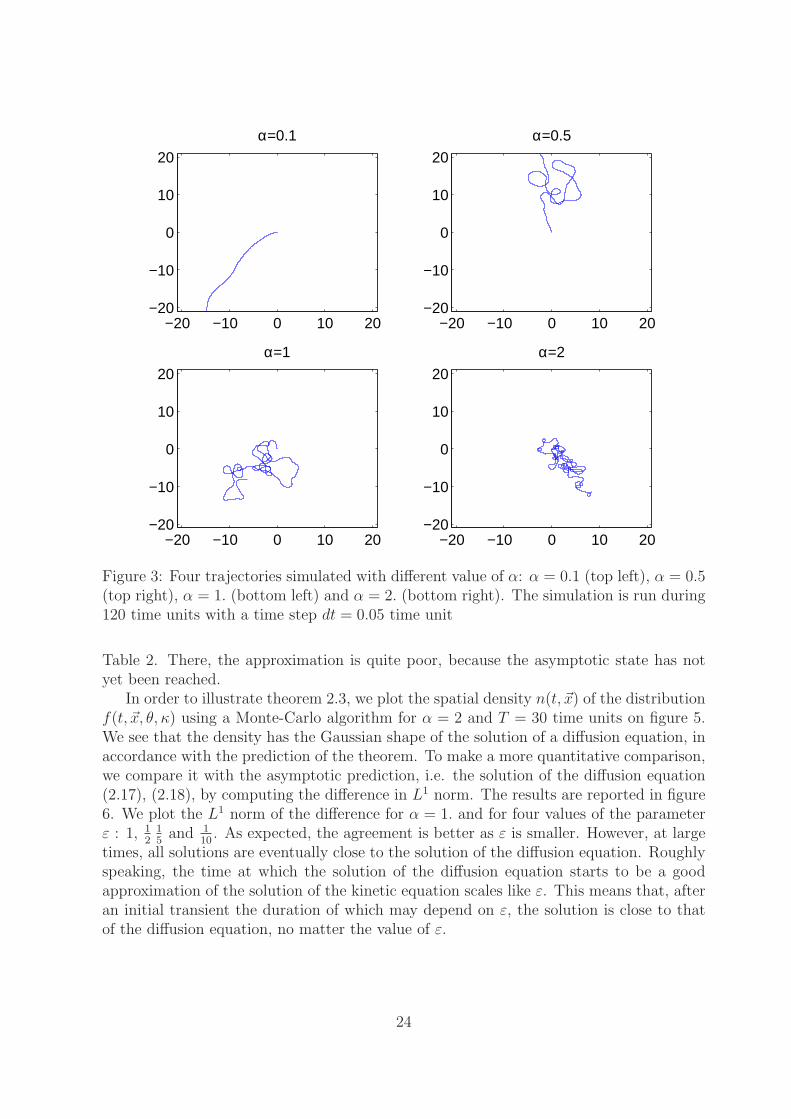
We present four trajectories obtained with different values of the parameter α infigure 3. As the parameter α increases, the excursions towards large positive or negativecurvatures become larger. As a consequence, the spinning of the trajectory around itselfincreases and, from almost a straight line when α = 0.1, the trajectory shrinks and lookscloser and closer to a wool ball. In this way, we can visualize the decay of D with respectto α.
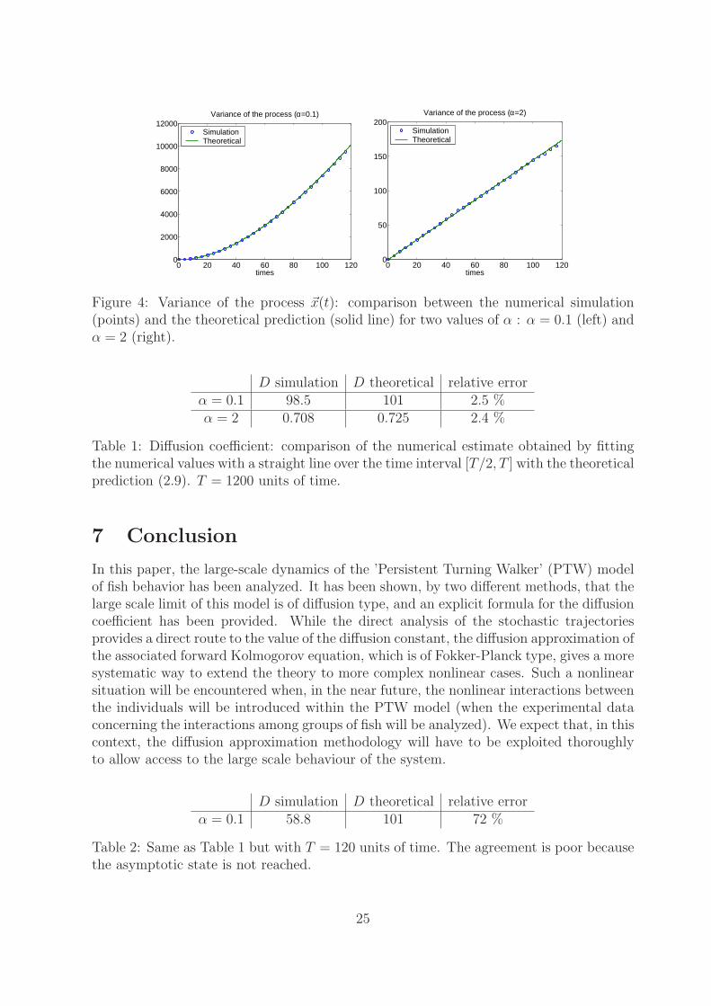
To illustrate theorem 2.1, we use a Monte-Carlo method to simulate the variance ofthe process ~x. We simulate N independent trajectories and we compute the varianceof the sample at each time step. In figure (4), we compare the result obtained withN = 2000 and the theoretical prediction given by the (3.6). The figure shows an excellentagreement between the computation and the theoretical prediction. Additionally, after aninitial transient, the growth of the variance is linear, in accordance with the theoreticalresult (2.9). We can use the slope of the asymptotically linear part of the curve to give anumerical estimate of the diffusion coefficient D. Fro this purpose, we fit a straight line(in the mean-square sense) between times T/2 and T . We remove the data between 0 andT/2 because the initial transient is not linear and including them would deteriorate theaccuracy of the measurement. We compare the slope of the fitted line with the theoreticalvalue (2.9). We report the result of this comparison for two values of α (α = 0.1 andα = 2., with T = 1200 time units in Table 1). The approximation is quite good, withan error comprised between 2 and 3%, which can be attributed to numerical noise and toan unsufficient approximation of the asymptotic state. To illustrate the influence of theinitial transient, we take T = 120 time units in the case α = 0.1 and report the result in
23
−20 −10 0 10 20−20
−10
0
10
20
α=0.1
−20 −10 0 10 20−20
−10
0
10
20
α=0.5
−20 −10 0 10 20−20
−10
0
10
20
α=1
−20 −10 0 10 20−20
−10
0
10
20
α=2
Figure 3: Four trajectories simulated with different value of α: α = 0.1 (top left), α = 0.5(top right), α = 1. (bottom left) and α = 2. (bottom right). The simulation is run during120 time units with a time step dt = 0.05 time unit
Table 2. There, the approximation is quite poor, because the asymptotic state has notyet been reached.
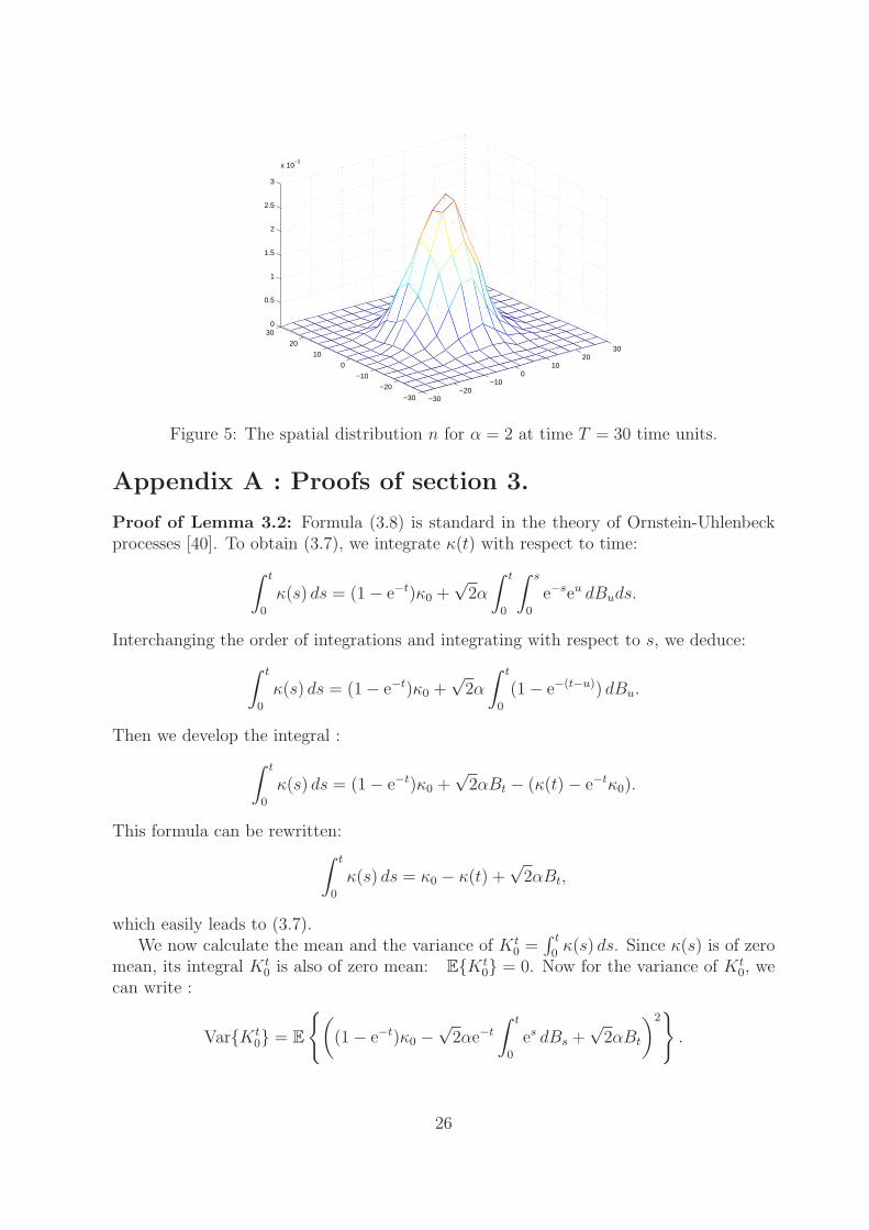
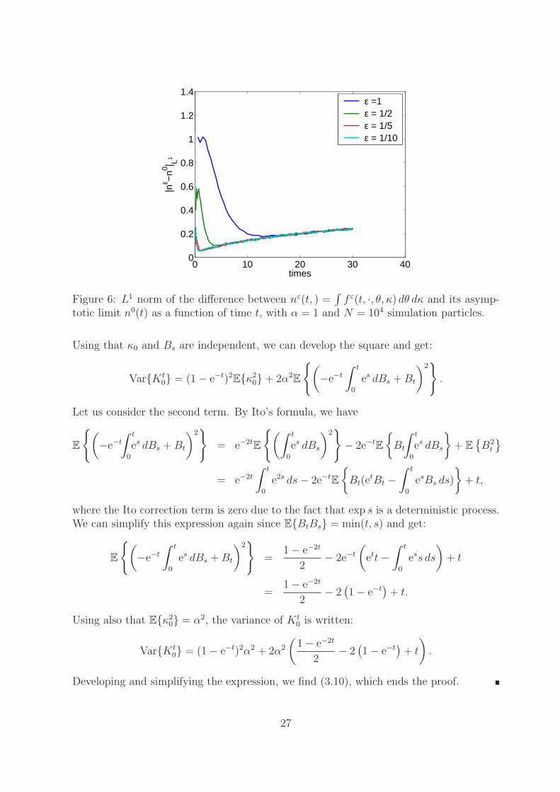
In order to illustrate theorem 2.3, we plot the spatial density n(t, ~x) of the distributionf(t, ~x, θ, κ) using a Monte-Carlo algorithm for α = 2 and T = 30 time units on figure 5.We see that the density has the Gaussian shape of the solution of a diffusion equation, inaccordance with the prediction of the theorem. To make a more quantitative comparison,we compare it with the asymptotic prediction, i.e. the solution of the diffusion equation(2.17), (2.18), by computing the difference in L1 norm. The results are reported in figure6. We plot the L1 norm of the difference for α = 1. and for four values of the parameterε : 1, 1
215and 1
10. As expected, the agreement is better as ε is smaller. However, at large
times, all solutions are eventually close to the solution of the diffusion equation. Roughlyspeaking, the time at which the solution of the diffusion equation starts to be a goodapproximation of the solution of the kinetic equation scales like ε. This means that, afteran initial transient the duration of which may depend on ε, the solution is close to thatof the diffusion equation, no matter the value of ε.
24
0 20 40 60 80 100 1200
2000
4000
6000
8000
10000
12000Variance of the process (α=0.1)
times
SimulationTheoretical
0 20 40 60 80 100 1200
50
100
150
200Variance of the process (α=2)
times
SimulationTheoretical
Figure 4: Variance of the process ~x(t): comparison between the numerical simulation(points) and the theoretical prediction (solid line) for two values of α : α = 0.1 (left) andα = 2 (right).
D simulation D theoretical relative errorα = 0.1 98.5 101 2.5 %α = 2 0.708 0.725 2.4 %
Table 1: Diffusion coefficient: comparison of the numerical estimate obtained by fittingthe numerical values with a straight line over the time interval [T/2, T ] with the theoreticalprediction (2.9). T = 1200 units of time.
7 Conclusion
In this paper, the large-scale dynamics of the ’Persistent Turning Walker’ (PTW) modelof fish behavior has been analyzed. It has been shown, by two different methods, that thelarge scale limit of this model is of diffusion type, and an explicit formula for the diffusioncoefficient has been provided. While the direct analysis of the stochastic trajectoriesprovides a direct route to the value of the diffusion constant, the diffusion approximation ofthe associated forward Kolmogorov equation, which is of Fokker-Planck type, gives a moresystematic way to extend the theory to more complex nonlinear cases. Such a nonlinearsituation will be encountered when, in the near future, the nonlinear interactions betweenthe individuals will be introduced within the PTW model (when the experimental dataconcerning the interactions among groups of fish will be analyzed). We expect that, in thiscontext, the diffusion approximation methodology will have to be exploited thoroughlyto allow access to the large scale behaviour of the system.
D simulation D theoretical relative errorα = 0.1 58.8 101 72 %
Table 2: Same as Table 1 but with T = 120 units of time. The agreement is poor becausethe asymptotic state is not reached.
25
−30−20
−100
1020
30
−30
−20
−10
0
10
20
300
0.5
1
1.5
2
2.5
3
x 10−3
Figure 5: The spatial distribution n for α = 2 at time T = 30 time units.
Appendix A : Proofs of section 3.
Proof of Lemma 3.2: Formula (3.8) is standard in the theory of Ornstein-Uhlenbeckprocesses [40]. To obtain (3.7), we integrate κ(t) with respect to time:
∫ t
0
κ(s) ds = (1− e−t)κ0 +√2α
∫ t
0
∫ s
0
e−seu dBuds.
Interchanging the order of integrations and integrating with respect to s, we deduce:
∫ t
0
κ(s) ds = (1− e−t)κ0 +√2α
∫ t
0
(1− e−(t−u)) dBu.
Then we develop the integral :
∫ t
0
κ(s) ds = (1− e−t)κ0 +√2αBt − (κ(t)− e−tκ0).
This formula can be rewritten:∫ t
0
κ(s) ds = κ0 − κ(t) +√2αBt,
which easily leads to (3.7).We now calculate the mean and the variance of Kt
0 =∫ t
0κ(s) ds. Since κ(s) is of zero
mean, its integral Kt0 is also of zero mean: E{Kt
0} = 0. Now for the variance of Kt0, we
can write :
Var{Kt0} = E
{
(
(1− e−t)κ0 −√2αe−t
∫ t
0
es dBs +√2αBt
)2}
.
26
0 10 20 30 400
0.2
0.4
0.6
0.8
1
1.2
1.4
times
|nε −
n0 | L1
ε =1ε = 1/2ε = 1/5ε = 1/10
Figure 6: L1 norm of the difference between nε(t, ) =∫
f ε(t, ·, θ, κ) dθ dκ and its asymp-totic limit n0(t) as a function of time t, with α = 1 and N = 104 simulation particles.
Using that κ0 and Bs are independent, we can develop the square and get:
Var{Kt0} = (1− e−t)2E{κ2
0}+ 2α2E
{
(
−e−t
∫ t
0
es dBs +Bt
)2}
.
Let us consider the second term. By Ito’s formula, we have
E
{
(
−e−t
∫ t
0
es dBs + Bt
)2}
= e−2tE
{
(∫ t
0
es dBs
)2}
− 2e−tE
{
Bt
∫ t
0
es dBs
}
+ E{
B2t
}
= e−2t
∫ t
0
e2s ds− 2e−tE
{
Bt(etBt −
∫ t
0
esBs ds)
}
+ t,
where the Ito correction term is zero due to the fact that exp s is a deterministic process.We can simplify this expression again since E{BtBs} = min(t, s) and get:
E
{
(
−e−t
∫ t
0
es dBs + Bt
)2}
=1− e−2t
2− 2e−t
(
ett−∫ t
0
ess ds
)
+ t
=1− e−2t
2− 2
(
1− e−t)
+ t.
Using also that E{κ20} = α2, the variance of Kt
0 is written:
Var{Kt0} = (1− e−t)2α2 + 2α2
(
1− e−2t
2− 2
(
1− e−t)
+ t
)
.
Developing and simplifying the expression, we find (3.10), which ends the proof.
27
Appendix B : Proofs of section 4.
Proof of Lemma 4.3: Let u ∈ D(A). Then, κ∂θu ∈ V ′ and Lemma A1 of [15] showsthat the Green formula for functions u ∈ V such that κ∂θu ∈ V ′ is legitimate. Therefore,taking the inner product of A(u) against u, we find:
< A(u), u >H=
∫
θ,κ
α2M∣
∣
∣∂κ
( u
M
)∣
∣
∣
2
dθdκ ≥ 0. (7.1)
So, A is a monotone operator in H. To show that A is maximal monotone, we prove thatfor any g ∈ H, there exists u ∈ D(A) such that :
u+ Au = g. (7.2)
Taking the inner product of (7.2) against a test function ϕ in the space D(Πθ × Rκ)of infinitely differentiable and compactly supported functions on Πθ × Rκ leads to thevariational problem :
∫
κ,θ
[u (ϕ− κ∂θϕ)1
M+ M∂k
( u
M
)
∂k
( ϕ
M
)
] dθdκ =
∫
θ,κ
gϕdκdθ
M. (7.3)
Again, the same theory as in the appendix A of [15] (based the result by J. L. Lions in[37]) applies to prove the existence of a solution to (7.3) with u in V such that κ∂θu ∈ V ′.From there, it immediately follows that u ∈ D(A).
It is immediate to see that any function of the form u(θ, κ) = CM(κ) for any constantC belongs to the kernel of A. Conversely, suppose that u ∈ KerA. Then, by (7.1), thereexists a function C(θ) ∈ L2(Π) such that u(θ, κ) = C(θ)M(κ). But again, A(u) = 0implies that κ ∂θC(θ)M = 0. So C(θ) is a constant, which proves (4.23).
Proof of Proposition 4.5: The ’only if’ part of the theorem is obvious since, us-ing Green’s formula (again, obtained by adapting that of appendix B of [15], we have∫
Audθ dκ = 0).To prove the ’if’ part, we borrow a method from (for instance) [12]. To find a solution
to (4.24), we look at a perturbed equation :
λu+ Au = g, (7.4)
with λ > 0. Since A is maximal monotone in H (Lemma 4.3), eq. (7.4) admits a solutionuλ for all positive λ ([9]). To prove the existence of a solution to (4.24), we want to extracta subsequence, still denoted by (uλ) which converges weakly in H. For this purpose, it isenough to show that there exists a bounded subsequence.
We proceed by contradiction, supposing that the (full) sequence Nλ = ‖uλ‖H λ→0→ +∞.We define Uλ = uλ
Nλ. Uλ satisfies ‖Uλ‖H = 1 for all λ and
λUλ + AUλ =g
Nλ
. (7.5)
Since (Uλ)λ is a bounded sequence in H, we can extract a subsequence (still denoted byUλ) such that Uλ ⇀ U in H weak as λ → 0. Taking the limit λ → 0 in (7.5), gives
28
A(U) = 0. If we take the inner product of (7.5) with Uλ and then pass to the limitλ → 0, we also find that U belongs to V . So Lemma 4.3 applies and gives U = cM witha constant c ∈ R. Using (4.25), we also have :
< λUλ + AUλ,M >H=<g
Nλ
,M >H= 0.
So∫
κ,θUλ dθdκ = 0 for all λ. Taking the limit λ → 0 leads to
∫
κ,θU dθdκ =
∫
κ,θCM(κ) dθdκ = 2πC = 0, which implies U = 0. This proves:
Uλ ⇀ 0 in H weak . (7.6)
To get a contradiction, we now prove that the convergence is strong.To this aim, we introduce a decomposition of the space H into two orthogonal sub-
spaces. Let L be the closed subspace of H defined by :
L = {c(θ)M / c(θ) ∈ L2(Πθ)},
with M defined by (4.4). So H = L⊥⊕ L⊥. We also define the orthogonal projector P
of H onto L such that Pf =(∫
κf(κ, θ) dκ
)
M . Using this projection, we decompose thesequence (Uλ)λ as follows:
Uλ = cλ(θ)M + vλ, (7.7)
with vλ ∈ L⊥, i.e.∫
κvλ dκ = 0. To demonstrate that Uλ
λ→0−→ 0 in H strongly, we first
demonstrate that vλλ→0−→ 0 in H strongly.
Taking the inner product of the equation satisfied by Uλ (7.5) with Uλ gives :
λ‖Uλ‖2H +
∫
θ,κ
M
∣
∣
∣
∣
∂κUλ
M
∣
∣
∣
∣
2
dθdκ =1
Nλ
< g, Uλ >H .
Since ∂κUλ
M= ∂κ
vλM
and ‖Uλ‖H = 1, we get by taking the limit λ → 0 :
∫
θ,κ
M∣
∣
∣∂κ
vλM
∣
∣
∣
2
dθdκλ→0−→ 0. (7.8)
Now Gross inequality [32] gives, for any v ∈ V :
α2
∫
R
∣
∣
∣
∣
∂κ
(
f
M
)∣
∣
∣
∣
2
M dκ ≥∫
R
|f |2 dκM
−(∫
R
f dκ
)2
. (7.9)
Then, since∫
κvλ dκ = 0, we deduce:
α2
∫
R
∣
∣
∣∂κ
vλM
∣
∣
∣
2
M dκ ≥∫
R
|vλ|2M
dκ.
Integrating this inequality with respect to θ and using (7.8), we find:
‖vλ‖H λ→0−→ 0, in H strong. (7.10)
29
To prove the convergence of cλ, we define the bounded operator T : H → L2(Πθ) suchthat Tf =
∫
κκf dκ. Having T acting on (7.5) and taking the limit λ → 0, leads to:
T AUλλ→0−→ 0 in L2(Πθ) strong. (7.11)
If we develop the left-hand side, we find:
T AUλ =
∫
κ
κ2∂θUλ dκ−∫
κ
[
κ∂κ(κUλ)− α2κ∂κ2Uλ
]
dκ
=
∫
κ
κ2∂θUλ dκ+
∫
κ
κUλ dκ.
But using the decomposition Uλ = cλM + vλ (7.7), we have:
∥
∥
∥
∥
∫
κ
κUλ dκ
∥
∥
∥
∥
L2(θ)
=
∥
∥
∥
∥
∫
κ
κvλ dκ
∥
∥
∥
∥
L2(θ)
λ→0−→ 0.
So, (7.11) leads to :∫
κ
κ2∂θUλ dκλ→0−→ 0 in L2(Πθ) strong. (7.12)
If we define hλ(θ) =∫
κκ2Uλ dκ, (7.12) is equivalent to saying that ‖∂θhλ‖L2(θ)
λ→0−→ 0.Using the Poincare-Wirtinger inequality [9], there exists a constant C0 such that:
‖hλ − hλ‖L2(θ) ≤ C0‖∂θhλ‖L2(θ), (7.13)
with hλ = 12π
∫ 2π
0hλ(θ) dθ. Then, we develop hλ. We get:
hλ =1
2π
∫ 2π
0
∫
κ
κ2Uλ dκdθ =< Uλ,Mκ2 >Hλ→0−→ 0 in R,
since Uλ converges weakly to zero (see (7.6)). So, (7.13) leads to hλλ→0−→ 0 in L2(Πθ)
strong. If we develop hλ we find:
hλ(θ) =
∫
κ
κ2(cλ(θ)M + vλ) dκ = α2cλ(θ) +
∫
κ
κ2vλ dκ.
Now,∫
κκ2vλ dκ converges to zero in L2(θ) strong because of (7.10) and we finally have :
cλ(θ)λ→0−→ 0 in L2(θ) strong.
Using the convergence of cλ and vλ, we can now prove the strong convergence of Uλ
to 0 in H:‖Uλ‖2H = ‖cλM‖2H + ‖vλ‖2H = ‖cλ‖2L2(θ) + ‖vλ‖2H
λ→0−→ 0,
which contradicts the fact that Uλ has unit norm in H. This shows that there exists abounded subsequence in the sequence uλ. In fact, since the same proof can be applied to
30
any subsequence, this shows that the whole sequence uλ is bounded, but this is uselessfor our purpose.
We conclude the proof of Proposition 4.5 as follows: there exists a subsequence uλ anda function u in H such that uλ ⇀ u in H weak. Taking the limit of (7.4) as λ → 0, wededuce that Au = g in the sense of distributions. However, since g ∈ H, eq. Au = g alsoholds in H. Moreover if we take the inner product of (7.4) with uλ and pass to the limitλ → 0, we find that u belongs to V . So u belongs to D(A), which ends the proof of the’if’ part of the statement.
Finally, to prove uniqueness, we just remark that, two solutions of (4.24) differ froman element of the kernel of A and we apply (4.23). This ends the proof.
31
Appendix C : Proofs of section 5.
Proof of Lemma 5.1: The proof borrows some ideas from [24], but is simpler, due tothe linear character of the problem. The difficulty is getting some compactness in time.Here, instead of considering time translates of the solution as in [24], we will considertime integrals over a fixed interval length ∆t.
Since operator A is maximal monotone on H (see Lemma 4.3), operator −A generatesa semi-group of contractions Tt on H. Moreover the solution of (5.1) is given by:
u(t) = Tt(u0) +
∫ t
0
Ts(g) ds.
We define f(t) = u(t)− u∞ which satisfies :
∂tf = −Af, ft=0 = f0, (7.14)
with f0 = u0 − u∞ and∫
κf0(κ) dκ = 0. To prove the weak convergence of u(t) to u∞, we
have to prove that f(t) converges to zero weakly in H.To this aim, we make an orthogonal decomposition of f(t) as in the proof of Proposition
4.5: f(t) = c(t)M + v(t), with c(t) ∈ L2(Πθ), v(t) ∈ H and∫
κv(t) dκ = 0. Taking the
inner product of (7.14) with f , we get :
1
2∂t‖f‖2H = −
∫
κ,θ
α2M
[
∂κ
(
f
M
)]2
dκdθ.
Using the decomposition of f(t) and noticing that ∂κ(
f
M
)
= ∂κ(
vM
)
, this equality be-comes:
1
2∂t(
‖c(t)‖2L2 + ‖v(t)‖2H)
= −∫
κ,θ
α2M
[
∂κ
(
v(t)
M
)]2
dκdθ. (7.15)
If we apply the Gross inequality (7.9), we get:
1
2∂t(
‖c(t)‖2L2 + ‖v(t)‖2H)
≤ −‖v(t)‖2H .
Since c(t) is bounded by ‖f0‖2H , by integrating with respect to time, we have :
1
2‖v(t)‖2H ≤ −
∫ t
0
‖v(s)‖2H ds+ C.
Using the Gronwall lemma, we deduce that v(t) decays exponentially fast to zero stronglyin H:
v(t)t→+∞−→ 0 in H strong.
It remains to prove the convergence of c(t) to zero. We integrate (7.14) with respectto κ. This gives, using that
∫
κM(κ) dκ = 1 and
∫
κv(t) dκ = 0 :
∂tc(t) = ∂θ
∫
κ
κv(t) dκ. (7.16)
32
Now if we pre-multiply by κ before integrating with respect to κ, we obtain :
∂t
∫
κ
κv(t) dκ = α2∂θc(t) + ∂θ
∫
κ
κ2v(t) dκ−∫
κ
κv(t) dκ. (7.17)
We fix a time interval ∆t and integrate (7.17) over this time interval. This leads to:∫
κ
κ(v(t+∆t)− v(t)) dκ = α2∂θ
∫ t+∆t
t
c(s) ds+ ∂θ
∫
κ
κ2
∫ t+∆t
t
v(s) ds dκ
−∫
κ
κ
∫ t+∆t
t
v(s) ds dκ.
Since v(t) converges to zero in H, we have, in the sense of distributions:
α2∂θ
∫ t+∆t
t
c(s) dst→+∞⇀ 0. (7.18)
Since c belongs to L∞((0,∞)t, L2(Πθ)) (see (7.15)), we have
∫ t+∆t
tc(s) ds which belongs
toL∞((0,∞)t, L
2(Πθ)). So there exists a subsequence such that∫ t+∆t
tc(s) ds is weakly
convergent in L2(Πθ). Actually, (7.18) implies that there exists a constant function withrespect to θ, depending on ∆t and denoted by L(∆t) such that
∫ t+∆t
t
c(s) dst→+∞⇀ L(∆t).
To deduce the convergence of c(t), we have to control the derivative of c(t) in time. Forthis purpose, we rewrite :
∫ t+∆t
t
c(s) ds =
∫ ∆t
0
(
c(t) +
∫ s
0
∂tc(t+ z) dz
)
ds
= ∆t c(t) +
∫ ∆t
0
∫ s
0
∂θ
∫
κ
κv(t+ z) dκ dzds.
Using again the convergence of v(t) to zero, we find :
∆t c(t)t→+∞⇀ L(∆t),
or defining the constant C = L(∆t)∆t
, we have c(t)t→+∞⇀ C in L2(Πθ) weak.
To complete the proof, it remains to prove that C is equal to zero. Now, since eq.(7.14) is mass preserving i.e.:
∂t
∫
κ,θ
f(t) dκdθ = −∫
κ,θ
Af(t) dκdθ = 0,
we have∫
κ,θf(t) dκdθ =
∫
κ,θf(0) dκdθ = 0. Also :
∫
κ,θ
f(t) dκdθ =
∫
κ,θ
(c(t)M + v(t)) dκdθt→+∞⇀
∫
θ
C dθ2πC.
So C = 0. This proves f(t)t→+∞⇀ 0 in H weak and completes the proof.
33
References
[1] M. Aldana and C. Huepe, Phase transitions in self-driven many-particle systems andrelated non-equilibrium models: a network approach, J. Stat. Phys., 112, no 1/2(2003), pp. 135–153.
[2] I. Aoki, A simulation study on the schooling mechanism in fish, Bulletin of the JapanSociety of Scientific Fisheries, 48 (1982), pp. 1081–1088.
[3] D. Armbruster, P. Degond and C. Ringhofer, A model for the dynamics of largequeuing networks and supply chains, SIAM J. Appl. Math., 66 (2006), pp. 896–920.
[4] A. Aw, A. Klar, M. Rascle and T. Materne, Derivation of continuum traffic flowmodels from microscopic follow-the-leader models, SIAM J. Appl. Math., 63 (2002),pp. 259–278.
[5] R. Bass, Diffusions and elliptic operators, Springer-Verlag, 1997.
[6] C. Bardos, R. Santos and R. Sentis, Diffusion approximation and computation of thecritical size, Trans. A. M. S., 284 (1984), pp. 617–649.
[7] N. Ben Abdallah, P. Degond, A. Mellet and F. Poupaud, Electron transport insemiconductor superlattices, Quarterly Appl. Math. 61 (2003), pp. 161–192.
[8] A. Bensoussan, J. L. Lions and G. C. Papanicolaou, Boundary layers and homoge-nization of transport processes, J. Publ. RIMS Kyoto Univ. 15 (1979), pp. 53–157.
[9] H. Brezis, Analyse fonctionnelle, Dunod, 1983.
[10] D. R. Brillinger, H. K. Preisler, A. A. Ager, J. G. Kie and B. S. Stewart, Employingstochastic differential equations to model wildlife motion, Bull Braz Math Soc, 33(2002), pp. 385–408.
[11] S. Camazine, J-L. Deneubourg, N. R. Franks, J. Sneyd, G. Theraulaz and E.Bonabeau, Self-Organization in Biological Systems, Princeton University Press, 2002.
[12] F. Castella, P. Degond and T. Goudon, Diffusion dynamics of classical systems drivenby an oscillatory force, J. Stat. Phys., 124 (2006), pp. 913–950.
[13] C. Cercignani, R. Illner, M. Pulvirenti, The mathematical theory of dilute gases,Springer-Verlag, New-York, 1991.
[14] I. D. Couzin, J. Krause, R. James, G. D. Ruxton and N. R. Franks, CollectiveMemory and Spatial Sorting in Animal Groups, J. theor. Biol., 218 (2002), pp. 1–11.
[15] P. Degond, Global Existence of Solutions for the Vlasov-Fokker-Planck Equation in1 and 2 Space Dimensions, An. Scient. Ec. Norm. Sup., 19 (1986) pp. 519-542.
34
[16] P. Degond, Macroscopic limits of the Boltzmann equation: a review, in Modeling andcomputational methods for kinetic equations, P. Degond, L. Pareschi, G. Russo (eds),Modeling and Simulation in Science, Engineering and Technology Series, Birkhauser,2003, pp. 3–57.
[17] P. Degond, V. Latocha, S. Mancini, A. Mellet, Diffusion dynamics of an electron gasconfined between two plates, Methods and Applications of Analysis. 9 (2002), pp.127–150.
[18] P. Degond, M. Lemou, M. Picasso, Viscoelastic fluid models derived from kineticequations for polymers, SIAM J. Appl. Math. 62 (2002), pp. 1501–1519.
[19] P. Degond et S. Mancini, Diffusion driven by collisions with the boundary, Asymp-totic Analysis 27 (2001), pp. 47–73.
[20] P. Degond, S. Mas-Gallic, Existence of Solutions and Diffusion Approximation for aModel Fokker-Planck Equation, Transp. Theory Stat. Phys., 16 (1987) pp. 589-636.
[21] P. Degond and S. Motsch, Continuum limit of self-driven particles with orientationinteraction, to appear in Mathematical Models and Methods in Applied Sciences(M3AS).
[22] P. Degond and S. Motsch, Macroscopic limit of self-driven particles with orientationinteraction, C. R. Acad. Sci. Paris, Ser. I 345 (2007), pp. 555–560.
[23] P. Degond et K. Zhang, Diffusion approximation of a scattering matrix model of asemiconductor superlattice, SIAM J. Appl. Math. 63 (2002), pp. 279–298.
[24] L. Desvillettes and J. Dolbeault,m On Long Time Asymptotics of the Vlasov-Poisson-Boltzmann Equation, Comm. PDE, 16 (1991), pp. 451–489.
[25] M. R. D’Orsogna, Y. L. Chuang, A. L. Bertozzi and L. Chayes, Self-propelled par-ticles with soft-core interactions: patterns, stability and collapse, Phys. Rev. Lett.,2006.
[26] L. Edelstein-Keshet, Mathematical models of swarming and social aggregation, in-vited lecture, The 2001 International Symposium on Nonlinear Theory and its Ap-plications, (NOLTA 2001) Miyagi, Japan (Oct 28-Nov 1, 2001).
[27] B. M. Friedrich and F. Julicher, Chemotaxis of sperm cells, PNAS 104 (2007), pp.13256–13261.
[28] J. Gautrais, S. Motsch, C. Jost, M. Soria, A. Campo, R. Fournier, S. Bianco and G.Theraulaz, Analyzing fish movement as a persistent turning walker, in preparation.
[29] F. Golse and F. Poupaud, Limite fluide des equations de Boltzmann des semicon-ducteurs pour une statistique de Fermi-Dirac, Asymptotic Analysis 6 (1992), pp.135–160.
35
[30] I. S. Gradshteyn, I. M. Ryzhik, Tables of integrals, series and products, 6th edition,Academic Press, New-York, 2000
[31] G. Gregoire, and H. Chate, Onset of collective and cohesive motion, Phys. Rev. Lett.,92 (2004) 025702.
[32] L. Gross, Logarithmic Sobolev inequalities and contractivity properties of semi-groups, Lectures Notes in Mathematics, Vol. 1563, pp. 54–88, Springer, Berlin, 1992.
[33] D. Helbing, Traffic and related self-driven many-particle systems, Reviews of modernphysics, 73 (2001), pp. 1067–1141.
[34] R. Jeanson, S. Blanco, R., Fournier, J. L. Deneubourg, V. FourcassiA c© & G. Ther-aulaz, A model of animal movements in a bounded space, Journal of TheoreticalBiology, 225 (2003), pp. 443-451
[35] C. Jost et al., From individual to collective ant displacements in heterogenous envi-ronments, preprint, 2007.
[36] V. L. Kulinskii, V. I. Ratushnaya, A. V. Zvelindovsky, D. Bedeaux, Hydrodynamicmodel for a system of self-propelling particles with conservative kinematic constraints,Europhys. Lett., 71 (2005), pp. 207–213.
[37] J.L. Lions, Equations differentielles operationnelles et problemes aux limites,Springer-Verlag, 1961.
[38] A. Mogilner and L. Edelstein-Keshet, A non-local model for a swarm, J. Math. Biol.,38 (1999), pp. 534–570.
[39] A. Mogilner, L. Edelstein-Keshet, L. Bent and A. Spiros, Mutual interactions, po-tentials, and individual distance in a social aggregation, J. Math. Biol., 47 (2003),pp. 353–389.
[40] B. Oksendal, Stochastic differential equations, Springer-Verlag, 1992.
[41] H. G. Othmer and Thomas Hillen, The Diffusion Limit of Transport Equations II:Chemotaxis Equations, SIAM J. Appl. Math., 62 (2002), pp. 1222-1250.
[42] J. K. Parrish and S. V. Viscido, Traffic rules of fish schools: a review of agent-basedapproaches, in ’Self-Organization and Complexity’, CK Hemelrijk (ed.), CambridgeUniversity Press, 2003.
[43] J. K. Parrish, S. V. Viscido and D. Grunbaum, Self-organized fish schools: an exam-ination of emergent properties, The biological bulletin, 202 (2002), pp. 296–305.
[44] A. Pazy, Semigroups of linear operators and applications to partial differential equa-tions, Springer-Verlag, 1983.
[45] F. Poupaud, Diffusion approximation of the linear semiconductor equation: analysisof boundary layers, Asymptotic Analysis 4 (1991), pp. 293–317.
36
[46] V. I. Ratushnaya, D. Bedeaux, V. L. Kulinskii and A. V. Zvelindovsky, Collective be-haviour of self propelling particles with kinematic constraints ; the relations betweenthe discrete and the continuous description, Physica A, to appear.
[47] V. I. Ratushnaya, V. L. Kulinskii, A. V. Zvelindovsky, D. Bedeaux, Hydrodynamicmodel for the system of self propelling particles with conservative kinematic con-straints; two dimensional stationary solutions Physica A, 366, (2006), pp. 107–114.
[48] Theraulaz et al., Spatial patterns in ant colonies, Proceedings of the NationalAcademy of Sciences, 99 (2002), pp. 9645–9649.
[49] C. M. Topaz and A. L. Bertozzi, Swarming patterns in a two-dimensional kinematicmodel for biological groups, SIAM J. Appl. Math, 65 (2004), pp. 152–174.
[50] C. M. Topaz, A. L. Bertozzi, M. A. Lewis, A nonlocal continuum model for biologicalaggregation, Bull. Math. Biol., 68 (2006), pp. 1601–1623.
[51] T. Vicsek, A. Czirok, E. Ben-Jacob, I. Cohen and O. Shochet, Novel type of phasetransition in a system of self-driven particles, Phys. Rev. Lett., 75 (1995), pp. 1226–1229.
37