Large-Scale Analysis of Soccer Matches usingSpatiotemporal Tracking Data

Alina Bialkowski1,2, Patrick Lucey1, Peter Carr1, Yisong Yue1,3, Sridha Sridharan2 and Iain Matthews11Disney Research, Pittsburgh, USA, 2Queensland University of Technology, Australia, 3California Institute of Technology, USA

Email: a.bialkowski@connect.qut.edu.au, {patrick.lucey, peter.carr, iainm}@disneyresearch.comyyue@caltech.edu, s.sridharan@qut.edu.au

Abstract—Although the collection of player and ball trackingdata is fast becoming the norm in professional sports, large-scalemining of such spatiotemporal data has yet to surface. In thispaper, given an entire season’s worth of player and ball trackingdata from a professional soccer league (≈400,000,000 data points),we present a method which can conduct both individual playerand team analysis. Due to the dynamic, continuous and multi-player nature of team sports like soccer, a major issue isaligning player positions over time. We present a “role-based”representation that dynamically updates each player’s relativerole at each frame and demonstrate how this captures the short-term context to enable both individual player and team analysis.We discover role directly from data by utilizing a minimumentropy data partitioning method and show how this can be usedto accurately detect and visualize formations, as well as analyzeindividual player behavior.

I. INTRODUCTION

Coinciding with the widespread deployment of trackingtechnologies, an enormous amount of trajectory data loggingmovements of people, vehicles, animals and weather patternshas emerged for various applications such as transportation [1],military [2], social [3], scientific studies [4] and hurricaneprediction [5]. Another interesting application which has seena recent deluge of spatiotemporal tracking data is the domainof sports analytics, where vision-based tracking systems havebeen deployed in professional basketball [6], soccer [7], base-ball [8] tennis and cricket [9]. However, even though an enor-mous amount of data is being generated for visualization andumpiring consideration, few methods for large-scale analysisof the tracking data have surfaced.

In team sports, there are two types of analysis that canbe conducted: a) individual and b) team analysis. In termsof analyzing individual player behavior, current methods plotlocations of a particular player for an event or their meanposition over time [10]. However, such methods lack importantcontextual information with regards to their team-mates. Forexample in soccer (see Fig. 1(a)), given we have a playerwho starts on the left-wing but then half way through thehalf he switches to the right wing, we get two distinct typesof behaviors (i.e., left and right wing play). Current analysisconducts the analysis based on his original position or “role”(i.e., left-wing) which makes comparisons challenging. Ideally,we want a contextual label noting the player’s role at thatspecific moment (and not normal/starting position). To conductrole-specific analysis, we first need to define the set of roles.A role within a team can be defined as a space or areathat each player is assigned responsibility for relative to the

xxxxx

xxx xx

x

x

x xxxxx

xx xxxxxxxxx

xxxx

x

xxxxx

xxx xx

x

x

x xxxxx

xx xxxxxxxxx

xxxx

x

xMean MeanLWx

xMeanRW

(a) (b)

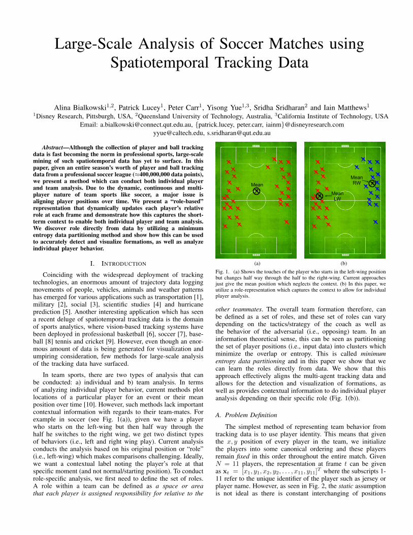
Fig. 1. (a) Shows the touches of the player who starts in the left-wing positionbut changes half way through the half to the right-wing. Current approachesjust give the mean position which neglects the context. (b) In this paper, weutilize a role-representation which captures the context to allow for individualplayer analysis.

other teammates. The overall team formation therefore, canbe defined as a set of roles, and these set of roles can varydepending on the tactics/strategy of the coach as well asthe behavior of the adversarial (i.e., opposing) team. In aninformation theoretical sense, this can be seen as partitioningthe set of player positions (i.e., input data) into clusters whichminimize the overlap or entropy. This is called minimumentropy data partitioning and in this paper we show that wecan learn the roles directly from data. We show that thisapproach effectively aligns the multi-agent tracking data andallows for the detection and visualization of formations, aswell as provides contextual information to do individual playeranalysis depending on their specific role (Fig. 1(b)).

A. Problem Definition

The simplest method of representing team behavior fromtracking data is to use player identity. This means that giventhe x, y position of every player in the team, we initializethe players into some canonical ordering and these playersremain fixed in this order throughout the entire match. GivenN = 11 players, the representation at frame t can be givenas xt = [x1, y1, x2, y2, . . . , x11, y11]

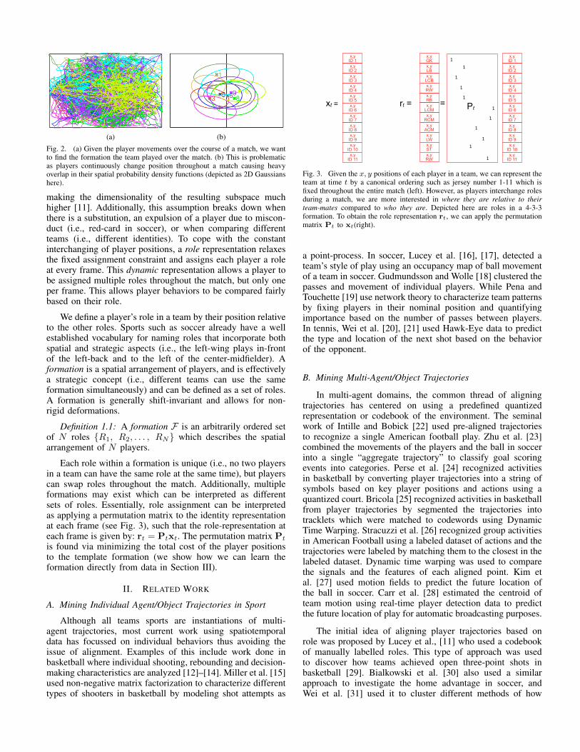
T where the subscripts 1-11 refer to the unique identifier of the player such as jersey orplayer name. However, as seen in Fig. 2, the static assumptionis not ideal as there is constant interchanging of positions

(a) (b)

Fig. 2. (a) Given the player movements over the course of a match, we wantto find the formation the team played over the match. (b) This is problematicas players continuously change position throughout a match causing heavyoverlap in their spatial probability density functions (depicted as 2D Gaussianshere).

making the dimensionality of the resulting subspace muchhigher [11]. Additionally, this assumption breaks down whenthere is a substitution, an expulsion of a player due to miscon-duct (i.e., red-card in soccer), or when comparing differentteams (i.e., different identities). To cope with the constantinterchanging of player positions, a role representation relaxesthe fixed assignment constraint and assigns each player a roleat every frame. This dynamic representation allows a player tobe assigned multiple roles throughout the match, but only oneper frame. This allows player behaviors to be compared fairlybased on their role.

We define a player’s role in a team by their position relativeto the other roles. Sports such as soccer already have a wellestablished vocabulary for naming roles that incorporate bothspatial and strategic aspects (i.e., the left-wing plays in-frontof the left-back and to the left of the center-midfielder). Aformation is a spatial arrangement of players, and is effectivelya strategic concept (i.e., different teams can use the sameformation simultaneously) and can be defined as a set of roles.A formation is generally shift-invariant and allows for non-rigid deformations.

Definition 1.1: A formation F is an arbitrarily ordered setof N roles {R1, R2, . . . , RN} which describes the spatialarrangement of N players.

Each role within a formation is unique (i.e., no two playersin a team can have the same role at the same time), but playerscan swap roles throughout the match. Additionally, multipleformations may exist which can be interpreted as differentsets of roles. Essentially, role assignment can be interpretedas applying a permutation matrix to the identity representationat each frame (see Fig. 3), such that the role-representation ateach frame is given by: rt = Ptxt. The permutation matrix Pt

is found via minimizing the total cost of the player positionsto the template formation (we show how we can learn theformation directly from data in Section III).

II. RELATED WORK

A. Mining Individual Agent/Object Trajectories in Sport

Although all teams sports are instantiations of multi-agent trajectories, most current work using spatiotemporaldata has focussed on individual behaviors thus avoiding theissue of alignment. Examples of this include work done inbasketball where individual shooting, rebounding and decision-making characteristics are analyzed [12]–[14]. Miller et al. [15]used non-negative matrix factorization to characterize differenttypes of shooters in basketball by modeling shot attempts as

11

1

1

1

1

1

11

1

xt"= =rt =

x,y GKx,yLBx,y

LCB

x,yRBx,y

LCMx,y

RCMx,y

ACMx,yLWx,ySTx,yRW

x,yRW

1

x,y ID 1x,y

ID 2x,y

ID 3x,y

ID 4x,y

ID 5x,y

ID 6x,y

ID 7x,y

ID 8x,y

ID 9x,y

ID 10x,y

ID 11

x,y ID 1x,y

ID 2x,y

ID 3x,y

ID 4x,y

ID 5x,y

ID 6x,y

ID 7x,y

ID 8x,y

ID 9x,y

ID 10x,y

ID 11

Pt

Fig. 3. Given the x, y positions of each player in a team, we can represent theteam at time t by a canonical ordering such as jersey number 1-11 which isfixed throughout the entire match (left). However, as players interchange rolesduring a match, we are more interested in where they are relative to theirteam-mates compared to who they are. Depicted here are roles in a 4-3-3formation. To obtain the role representation rt, we can apply the permutationmatrix Pt to xt(right).

a point-process. In soccer, Lucey et al. [16], [17], detected ateam’s style of play using an occupancy map of ball movementof a team in soccer. Gudmundsson and Wolle [18] clustered thepasses and movement of individual players. While Pena andTouchette [19] use network theory to characterize team patternsby fixing players in their nominal position and quantifyingimportance based on the number of passes between players.In tennis, Wei et al. [20], [21] used Hawk-Eye data to predictthe type and location of the next shot based on the behaviorof the opponent.

B. Mining Multi-Agent/Object Trajectories

In multi-agent domains, the common thread of aligningtrajectories has centered on using a predefined quantizedrepresentation or codebook of the environment. The seminalwork of Intille and Bobick [22] used pre-aligned trajectoriesto recognize a single American football play. Zhu et al. [23]combined the movements of the players and the ball in soccerinto a single “aggregate trajectory” to classify goal scoringevents into categories. Perse et al. [24] recognized activitiesin basketball by converting player trajectories into a string ofsymbols based on key player positions and actions using aquantized court. Bricola [25] recognized activities in basketballfrom player trajectories by segmented the trajectories intotracklets which were matched to codewords using DynamicTime Warping. Stracuzzi et al. [26] recognized group activitiesin American Football using a labeled dataset of actions and thetrajectories were labeled by matching them to the closest in thelabeled dataset. Dynamic time warping was used to comparethe signals and the features of each aligned point. Kim etal. [27] used motion fields to predict the future location ofthe ball in soccer. Carr et al. [28] estimated the centroid ofteam motion using real-time player detection data to predictthe future location of play for automatic broadcasting purposes.

The initial idea of aligning player trajectories based onrole was proposed by Lucey et al., [11] who used a codebookof manually labelled roles. This type of approach was usedto discover how teams achieved open three-point shots inbasketball [29]. Bialkowski et al. [30] also used a similarapproach to investigate the home advantage in soccer, andWei et al. [31] used it to cluster different methods of how

teams scored a goal. Although these works all align the multi-agent data is some form, our work differs as we learn thisalignment directly from the data.

III. ROLE DISCOVERY USING MINIMUM ENTROPY DATAPARTITIONING

A. Minimum Entropy Data Partitioning

Given player tracking data D, our goal is to estimatethe underlying formation of the team, which is equivalent tofinding the most probable set F∗ of 2D probability densityfunctions F∗ = argmaxF P (F|D). We begin by consideringthe 2D probability density function P (X = x) which modelsthe tracking data D. In other words, P (x) represents the heat-map for an entire team. We can model the heat-map of theentire team as a linear combination of the heat maps for eachrole

P (x) =

N∑n=1

P (x|n)P (n) (1)

=1

N

N∑n=1

Pn(x).

Strategically, a team needs to spread out its players so thatthe entire field is adequately covered. As a result, the prob-ability density functions should exhibit minimal overlap (seeFig. 4 (d)). Equivalently, each role probability density functionshould exhibit minimal overlap with the team’s probabilitydensity function. Following the ideas of minimum entropy datapartitioning [32], [33], we employ Kullback-Lieber divergenceto measure the overlap between two probability functions P (x)and Q(x)

KL(P (x)‖Q(x)) =

∫P (x) log

(P (x)

Q(x)

)dx. (2)

Since divergence is a strictly positive quantity (and com-pletely overlapping probability density functions have zerodivergence), we employ a penalty Vn based on the negativedivergence value between the heat map Pn(x) of an individualrole and that of the team P (x)

Vn = −KL(Pn(x)‖P (x)

). (3)

Computing the optimal formation F∗ is equivalent todetermining the optimal set F∗ = {P1(x), . . . , PN (x)}∗ ofper-role probability density functions Pn(x) that minimize thetotal overlap

F∗ = argminF

V. (4)

Substituting the expressions for KL divergence into thetotal overlap cost illustrates the dependence on each role-specific 2D probability density function

V = −N∑

n=1

P (n)

∫P (x|n) logP (x|n)dx

+

N∑n=1

P (n)

∫P (x|n) logP (x)dx. (5)

The expression for V is drastically simplified when put interms of entropy

H(x) = −∫ +∞

−∞P (x) log(P (x))dx. (6)

The total overlap cost, in terms of entropy, becomes

V = −H(x) +

N∑n=1

P (n)H(x|n) (7)

= −H(x) +1

N

N∑n=1

H(x|n). (8)

Substituting 8 into 4 and ignoring the constant term H(x),the optimal formation is the set of role-specific probabilitydensity functions that minimize the total entropy

F∗ = argminF

N∑n=1

H(x|n). (9)

B. Equivalence to K-Means

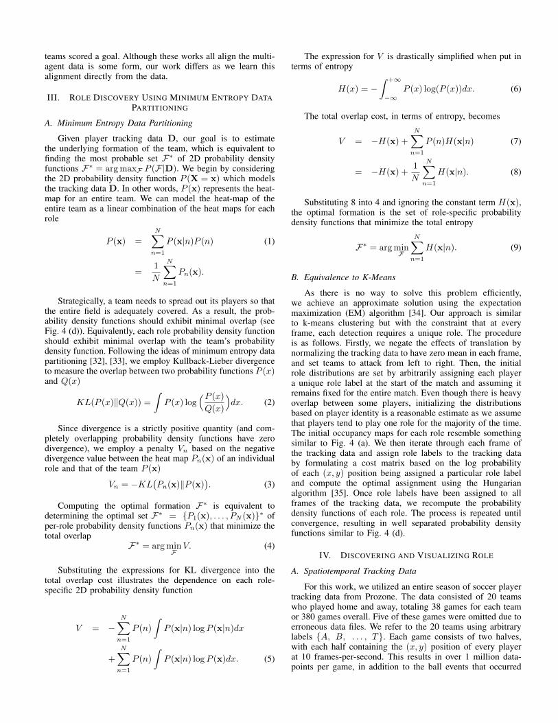
As there is no way to solve this problem efficiently,we achieve an approximate solution using the expectationmaximization (EM) algorithm [34]. Our approach is similarto k-means clustering but with the constraint that at everyframe, each detection requires a unique role. The procedureis as follows. Firstly, we negate the effects of translation bynormalizing the tracking data to have zero mean in each frame,and set teams to attack from left to right. Then, the initialrole distributions are set by arbitrarily assigning each playera unique role label at the start of the match and assuming itremains fixed for the entire match. Even though there is heavyoverlap between some players, initializing the distributionsbased on player identity is a reasonable estimate as we assumethat players tend to play one role for the majority of the time.The initial occupancy maps for each role resemble somethingsimilar to Fig. 4 (a). We then iterate through each frame ofthe tracking data and assign role labels to the tracking databy formulating a cost matrix based on the log probabilityof each (x, y) position being assigned a particular role labeland compute the optimal assignment using the Hungarianalgorithm [35]. Once role labels have been assigned to allframes of the tracking data, we recompute the probabilitydensity functions of each role. The process is repeated untilconvergence, resulting in well separated probability densityfunctions similar to Fig. 4 (d).

IV. DISCOVERING AND VISUALIZING ROLE

A. Spatiotemporal Tracking Data

For this work, we utilized an entire season of soccer playertracking data from Prozone. The data consisted of 20 teamswho played home and away, totaling 38 games for each teamor 380 games overall. Five of these games were omitted due toerroneous data files. We refer to the 20 teams using arbitrarylabels {A, B, . . . , T}. Each game consists of two halves,with each half containing the (x, y) position of every playerat 10 frames-per-second. This results in over 1 million data-points per game, in addition to the ball events that occurred

G691 T1, Iteration 13, diff = 0.00m

1

2

34

56

7

8

910

G691 T1, Iteration 2, diff = 3.77m

1

2

34

56

7

8

910

G691 T1, Iteration 1, diff = 13.17m

1

2

34

56

7

8

910

G691 T1, Initial Role Positions

1

2

34

56

7

8

9 10

G241 T1, Iteration 41, diff = 0.00m

12

3

4

56

7

8

9

10

G241 T1, Iteration 2, diff = 5.27m

1

2

3

4

56

7

8

9

10

G241 T1, Iteration 1, diff = 21.57m

1

2

3

4

56

7

8

9

10

G241 T1, Initial Role Positions

1

2

3

4

56

7

8

910

Initial Roles Iteration 1 Iteration 2 Final Roles...

(a) Initial Roles (b) Iteration 1 (c) Iteration 2 ... (d) Final Roles

Fig. 4. Example of our role discovery procedure for two teams showing the role distributions at each iteration (drawn as 2D gaussians). The initial roledistributions, (a), are calculated by assuming each player is assigned a single role over all frames and taking their distribution over the half. A high degreeof overlap is exhibited due to frequent positional swaps between players. Taking (a) as the template, each frame is assigned to these roles and the updateddistributions are shown in (b). This is then used as the template for the next iteration and the procedure is repeated until convergence, resulting in well separatedrole distributions as in (d).

throughout the match, consisting of 43 possible events (e.g.passes, shots, crosses, tackles etc.). Each of these ball eventscontains the time-stamp, location and players involved. Aninventory of the data is given in Table I.

B. Formation Detection

By using the expectation maximization procedure for min-imum entropy data partitioning described in Section III-B, wesimultaneously assign each player to a role at each frame ofthe tracking data and determine the role probability distribu-tions, Pn(x). We performed this procedure for each team andmatch half, excluding formations where players were sent off,resulting in the detection of 1411 formations. Each formationconsists of a set of ten distinct role probability distributionsrepresenting the structural arrangement of the team over a half,and depicts the long-term characteristic behavior of the team.

Given these role distributions, we then automatically dis-covered different types of formations. We employed agglom-erative clustering to group the discovered formations intoclusters, using the Earth Mover’s Distance (EMD) [36] tocompute the distance between two role probability densities.The EMD(a,b) between two normalized histograms a and bis obtained as the solution of the transportation problem

minfqt≥0

D∑q,t=1

dqtfqt s.t.∑D

q=1 fqt = at,∑D

t=1 fqt = bq. (10)

The variable fqt denotes a flow representing the amounttransported from the qth supply to the tth demand and dqt theground distance. Using the EMD measure gave us role-to-role

Statistic Frequency

Teams 20Games 375

Data Points 480MBall Events 981K

TABLE I. INVENTORY OF THE DATASET USED FOR THIS WORK.

50.37%20.76%

12.52%

5.40%

3.15%0.90%

Cluster 1 Cluster 2 Cluster 3

Cluster 4 Cluster 5 Cluster 6

Fig. 5. Formation clustering results displaying the mean role positions ofeach formation assigned to each cluster, and the median formation overlaid ingrey. (Note: all formations are set so that teams attack from left to right)

comparison distances, and then we set the distance betweenone formation and another equal to the sum of the distancesbetween corresponding roles.

The resulting clusters are shown in Fig. 5, with the meanrole positions of each formation overlaid over one another. Itcan be seen that clustering resulted in the discovery of distinctformation classes - e.g. Cluster 1 and 4 have only 1 strikerin the front, Cluster 2 and 6 have 2 strikers, while Cluster 3and 5 appear to have 3. Cluster 3 is the only cluster with 3defenders at the back with the remainder all having 4. Theclustering also gives an indication of which formations aremore commonly adopted by teams, as given by the clusteringassignment frequency (top right of each cluster in Fig. 5). Wecan see that Cluster 2, which appears to be a 4-4-2, is themost common with approximately 50.37% of formations beingassigned to this cluster, followed by Cluster 1 (20.76%), whichappears to be a 4-2-3-1. These give insight into the strategiesadopted by teams (e.g. having 2 strikers instead of 1 may beconsidered a more attacking strategy).

To evaluate the clustering results, we compare againstground truth formation labels, where a soccer expert annotatedthe dominant formation observed for each half and teamaccording to the arrangement of players (4-4-2, 4-2-3-1, 4-3-3,3-4-3, 4-1-4-1, or ‘other’ where the team either did not displaya dominant formation or was not one of the given labels). Toevaluate the results, we estimated the label of each cluster as

Confusion matrix

84

12

0

0

17

10

10

83

0

0

2

24

0

1

97

17

1

2

0

1

1

67

1

17

5

1

0

8

73

0

1

2

1

8

7

48

4−2−

3−1

4−4−

2

3−4−

3

4−3−

3

4−1−

4−1

Inte

rest

ing

4−2−3−1

4−4−2

3−4−3

4−3−3

4−1−4−1

Interesting

0

10

20

30

40

50

60

70

80

90

100

Ground Truth Formation Label

4-2-3-1

4-4-2

3-4-3

4-3-3

4-1-4-1

Other

1

2

3

4

5

6

Clu

ster

Num

ber

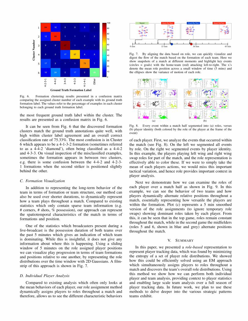
Fig. 6. Formation clustering results presented in a confusion matrixcomparing the assigned cluster number of each example with its ground truthformation label. The values refer to the percentage of examples in each clusterbelonging to each ground truth formation label.

the most frequent ground truth label within the cluster. Theresults are presented as a confusion matrix in Fig. 6.

It can be seen from Fig. 6 that the discovered formationclusters match the ground truth annotations quite well, withhigh within cluster label agreement and an overall correctclassification rate of 75.33%. The most confusion is in Cluster6 which appears to be a 4-1-3-2 formation (sometimes referredto as a 4-4-2 ‘diamond’), often being classified as a 4-4-2and 4-3-3. On visual inspection of the misclassified examples,sometimes the formation appears in between two clusters,e.g. there is some confusion between the 4-4-2 and 4-2-3-1 formations when the second striker is positioned slightlybehind the other.

C. Formation Visualization

In addition to representing the long-term behavior of theteam in terms of formation or team structure, our method canalso be used over shorter durations, to dynamically representhow a team plays throughout a match. Compared to existingstatistics which only contain sparse team information (e.g.# corners, # shots, % possession), our approach can representthe spatiotemporal characteristics of the match in terms offormations and position.

One of the statistics which broadcasters present during alive-broadcast is the possession duration of both teams overthe past 5 minutes which gives an indication of which teamis dominating. While this is insightful, it does not give anyinformation about where this is happening. Using a slidingwindow of 5 minutes on the role assigned player positionswe can visualize play progression in terms of team formationsand positions relative to one another, by representing the roledistributions over the time window with 2D Gaussians. A film-strip of this approach is shown in Fig. 7.

D. Individual Player Analysis

Compared to existing analysis which often only looks atthe mean behaviors of each player, our role assignment methoddynamically assigns players to roles throughout a match andtherefore, allows us to see the different characteristic behaviors

1

1

22

3

3

4

4

5

56

6

7

7 8

8

9

910

10

1

1

2

23

3

4

4

5

56

6

7

78

8

9

910

10

Neutral Attack: Red Team

1

1

2

23

3

4

4

556

6

7

78

89

9 10

10

Attack: Blue Team

1

1

2

233

4

4

55

6

6

7

7 8

8

99 10

10

Attack: Red Team

45 min30 min15 min0 min

Fig. 7. By aligning the data based on role, we can quickly visualize anddigest the flow of the match based on the formation of each team. Here weshow snapshots of a match at different moments and highlight key events(circles = goals) with the home-team (red) attacking left-to-right. The x’sdenote the mean role position across a small window of time (5 mins) andthe ellipses show the variance of motion of each role.

(a) (b)

Fig. 8. Every event within a match half segmented into (a) roles, versus(b) player identity (both colored by the role of the player at the frame of theevent)

of each player. First, we analyze the events that occurred withinthe match (see Fig. 8). On the left we segmented all eventsby role. On the right we segmented events by player identity.In this example, the players playing left wing and right wingswap roles for part of the match, and the role representation iseffectively able to color these. If we were to simply take themean of each players actions, we would miss this importanttactical variation, and hence role provides important context inplayer analysis.

Next we demonstrate how we can examine the roles ofeach player over a match half as shown in Fig. 9. In thisexample, we can see the behavior of two teams and howplayers dynamically alternate relative positions throughout amatch, essentially representing how versatile the players arewithin the formation. Plot (c) represents a 5 min smoothedversion of the role assignments (to ignore temporary roleswaps) showing dominant roles taken by each player. Fromthis, it can be seen that in the top game, roles remain constantthroughout the match, while in the second game the midfielders(roles 5 and 6, shown in blue and grey) alternate positionsthroughout the match.

V. SUMMARY

In this paper, we presented a role-based representation torepresent player tracking data, which was found by minimizingthe entropy of a set of player role distributions. We showedhow this could be efficiently solved using an EM approachwhich simultaneously assigns players to roles throughout amatch and discovers the team’s overall role distributions. Usingthis method we show how we can perform both individualplayer and team analysis, providing context to player statisticsand enabling large scale team analysis over a full season ofplayer tracking data. In future work, we plan to use thesemethods to delve deeper into the various strategic patternsteams exhibit.

LB

LCB

RCB

RB

DM

RCM

LW

RW

LCMST

LB LCB RCB RB DM LCM RCM LW RW ST

LB

LCB

RCB

RB

DM

LCM

RCM

LW

RW

ST

(a) (b) (c) (d)

LB

LCB

RCB

RB

LCM

RCM

LW

RW

ACM

ST

LB LCB RCB RB LCM RCM LW RW ACM ST

LB

LCB

RCB

RB

LCM

RCM

LW

RW

ACM

ST

Fig. 9. The behavior of two different teams over half a match, demonstrating: (a) Their overall formation calculated using our minimum entropy data partitioningmethod (with roles represented as 2D Gaussians). (b) A timeline showing the role assigned to each player at each frame, colored by role. (c) A 5 min smoothedversion of the role assignments (ignores temporary role swaps), (d) The per-frame role swaps across the half {left-back(LB), left-center-back(LCB), right-center-back(RCB), right-back(RB),left-centre-midfield(LCM), defensive-midfield(DM), right-centre-midfield(RCM), left wing(LW), right-wing(RW), attacking-center-midfielder(ACM), striker(ST)}

Acknowledgement: The QUT portion of this research was supported by theQld Govt’s Dept. of Employment, Economic Development & Innovation.

REFERENCES

[1] J. Yuan, Y. Zheng, C. Zhang, W. Xie, X. Xie, G. Sun, and Y. Huang,“T-Drive: Driving Directions based on Taxi Trajectories,” in GIS, 2010.

[2] L. Tang, X. Yu, S. Kim, J. Han, C. Hung, and W. Peng, “Tru-Alarm: Trustworthiness Analysis of Sensor Networks in Cyber-PhysicalSystems,” in ICDM, 2010.

[3] Y. Zheng, X. Xie, and W. Ma, “GeoLife: A Collaborative SocialNetworking Service Among User, Service ,” IEEE Data EngineeringBulletin, 2010.

[4] J. Gudmundsson and M. Krevald, “Computing Longest Duration Flocksin Trajectory Data,” in GIS, 2006.

[5] J. Lee, J. Han, and K. Whang, “Trajectory clustering: a partition-and-group framework,” in International Conference on Management ofData. ACM, 2007.

[6] STATS SportsVU, www.sportvu.com.[7] Prozone, www.prozonesports.com.[8] SportsVision, www.sportsvision.com.[9] Hawk-Eye, www.hawkeyeinnovations.co.uk.

[10] E. GameCast, http://www.espnfc.com/gamecast/392450/gamecast.html.[11] P. Lucey, A. Bialkowski, P. Carr, S. Morgan, I. Matthews, and Y. Sheikh,

“Representing and Discovering Adversarial Team Behaviors usingPlayer Roles,” in CVPR, 2013.

[12] K. Goldsberry, “CourtVision: New Visual and Spatial Analytics for theNBA,” in MIT SSAC, 2012.

[13] R. Masheswaran, Y. Chang, J. Su, S. Kwok, T. Levy, A. Wexler, andN. Hollingsworth, “The Three Dimensions of Rebounding,” in MITSSAC, 2014.

[14] D. Cervone, A. D’Amour, L. Bornn, and K. Goldsberry, “POINTWISE:Predicting Points and Valuing Decisions in Real Time with NBA OpticalTracking Data,” in MIT SSAC, 2014.

[15] A. Miller, L. Bornn, R. Adams, and K. Goldsberry, “Factorized PointProcess Intensities: A Spatial Analysis of Professional Basketball,” inICML, 2014.

[16] P. Lucey, A. Bialkowski, P. Carr, E. Foote, and I. Matthews, “Character-izing Multi-Agent Team Behavior from Partial Team Tracings: Evidencefrom the English Premier League,” in AAAI, 2012.

[17] P. Lucey, D. Oliver, P. Carr, J. Roth, and I. Matthews, “Assessing teamstrategy using spatiotemporal data,” in ACM SIGKDD, 2013.

[18] J. Gudmundsson and T. Wolle, “Football analysis using spatio-temporaltools,” Computers, Environment and Urban Systems, 2013.

[19] J. L. Pena and H. Touchette, “A network theory analysis of footballstrategies,” arXiv preprint arXiv:1206.6904, 2012.

[20] X. Wei, P. Lucey, S. Morgan, and S. Sridharan, “Sweet-Spot: UsingSpatiotemporal Data to Discover and Predict Shots in Tennis,” in MITSSAC, 2013.

[21] ——, “Predicting Shot Locations in Tennis using Spatiotemporal Data,”in DICTA, 2013.

[22] S. Intille and A. Bobick, “Recognizing Planned, Multi-Person Action,”CVIU, vol. 81, pp. 414–445, 2001.

[23] G. Zhu, Q. Huang, C. Xu, Y. Rui, S. Jiang, W. Gao, and H. Yao,“Trajectory based event tactics analysis in broadcast sports video,” inInternational Conference on Multimedia. ACM, 2007.

[24] M. Perse, M. Kristan, S. Kovacic, and J. Pers, “A Trajectory-BasedAnalysis of Coordinated Team Activity in Basketball Game,” CVIU,2008.

[25] J.-C. Bricola, “Classification of multi-agent trajectories,” Master’s the-sis, EPFL, 2012.

[26] D. Stracuzzi, A. Fern, K. Ali, R. Hess, J. Pinto, N. Li, T. Konik, andD. Shapiro, “An Application of Transfer to American Football: FromObservation of Raw Video to Control in a Simulated Environment,” AIMagazine, vol. 32, no. 2, 2011.

[27] K. Kim, M. Grundmann, A. Shamir, I. Matthews, J. Hodgins, andI. Essa, “Motion Fields to Predict Play Evolution in Dynamic SportsScenes,” in CVPR, 2010.

[28] P. Carr, M. Mistry, and I. Matthews, “Hybrid Robotic/Virtual Pan-Tilt-Zoom Cameras for Autonomous Event Recording,” in ACM Multimedia,2013.

[29] P. Lucey, A. Bialkowski, P. Carr, Y. Yue, and I. Matthews, “How to Getan Open Shot: Analyzing Team Movement in Basketball using TrackingData,” in MIT SSAC, 2014.

[30] A. Bialkowski, P. Lucey, P. Carr, Y. Yue, and I. Matthews, “Win athome and draw away: Automatic formation analysis highlighting thedifferences in home and away team behaviors,” in MIT SSAC, 2014.

[31] X. Wei, L. Sha, P. Lucey, S. Morgan, and S. Sridharan, “Large-ScaleAnalysis of Formations in Soccer,” in DICTA, 2013.

[32] S. Roberts, R. Everson, and I. Rezek, “Minimum Entropy Data Parti-tioning,” IET, 1999.

[33] Y. Lee and S. Choi, “Minimum Entropy, K-Means, Spectral Clustering,”in International Joint Conference on Neural Networks, 2004.

[34] A. Dempster, N. Laird, and D. Rubin, “Maximum Likelihood fromIncomplete Data via the EM Algorithm,” Journal of the Royal StatisticalSociety, vol. 39, no. 1, 1977.

[35] H. W. Kuhn, “The hungarian method for the assignment problem,”Naval Research Logistics Quarterly, vol. 2, no. 1-2, 1955.

[36] Y. Rubner, C. Tomasi, and L. Guibas, “A Metric for Distributions withApplications to Image Databases,” in ICCV, 1998.