Large-Array Signal Processing for Deep-Space Applications

IPN Progress Report 42-150 August 15, 2002

Large-Array Signal Processing forDeep-Space Applications

C. H. Lee,1 V. Vilnrotter,1 E. Satorius,1 Z. Ye,1 D. Fort,1 and K.-M. Cheung1

This article develops the mathematical models needed to describe the key issuesin using an array of antennas for receiving spacecraft signals for DSN applications.The detrimental effects of nearby interfering sources, such as other spacecraft trans-missions or natural radio sources within the array’s field of view, on signal-to noiseratio (SNR) are determined, atmospheric effects relevant to the arraying problemdeveloped, and two classes of algorithms (multiple signal classification (MUSIC)plus beam forming, and an eigen-based solution) capable of phasing up the ar-ray with maximized SNR in the presence of realistic disturbances are evaluated.It is shown that, when convolutionally encoded binary-phase shift keying (BPSK)data modulation is employed on the spacecraft signal, previously developed datapre-processing techniques that partially reconstruct the carrier can be of great ben-efit to array performance, particularly when strong interfering sources are present.Since this article is concerned mainly with demonstrating the required capabilitiesfor operation under realistic conditions, no attempt has been made to reduce algo-rithm complexity; the design and evaluation of less complex algorithms with similarcapabilities will be addressed in a future article. The performances of the candidatealgorithms discussed in this article have been evaluated in terms of the number ofsymbols needed to achieve a given level of combining loss for different numbers ofarray elements, and compared on this common basis. It is shown that even thebest algorithm requires approximately 25,000 symbols to achieve a combining lossof less than 0.5 dB when 128 antenna elements are employed, but generally 50,000or more symbols are needed. This is not a serious impediment to successful array-ing with high data-rate transmission, but may be of some concern with missionsexploring near the edge of our solar system or beyond, where lower data rates maybe required.

I. Introduction

Antenna arraying is an attractive technique for improving the reception of weak signals. Signalsreceived simultaneously from different antennas are combined in phase, effectively creating an equivalentlarger aperture. This approach can be of great benefit to deep-space communications where the spacecraftsignal is severely attenuated as it travels across vast interplanetary distances. With the enhanced signal-

1 Communications Systems and Research Section.

The research described in this publication was carried out by the Jet Propulsion Laboratory, California Institute ofTechnology, under a contract with the National Aeronautics and Space Administration.

1

to-noise ratio (SNR) obtained from an effectively larger aperture, arraying enables support of missionswhose signal level falls below the threshold of a single antenna. Alternatively, arraying can be usedto increase data return over that possible with a single antenna: for example, an array consisting offour hundred 5-m antennas can replace the 70-m antenna at Goldstone, the largest one in the network,without sacrificing any operational capabilities; in fact, the possibility of multibeaming, and gracefuldegradation in the event of equipment failure, actually enhances the value of large arrays for the DSN.The goal is to obtain a combined SNR at the array output of at least −5 dB (required for turbo codes),which corresponds to a −31 dB SNR at each antenna of a 400-element array.

This article examines various arraying techniques, focusing on the very low SNR conditions commonlyencountered in deep-space communications. In addition to achieving high combined SNR under idealconditions, these algorithms should also be able to operate under practical conditions, such as atmosphericturbulence over the array, and in the presence of spatially correlated interference from planets duringplanetary encounters or other sources of radio frequency interference (RFI). Adaptive beam-formingtechniques provide a flexible system to combat channel impairment typically encountered during planetaryencounter reception, and also provide additional capabilities not available with single large antennas.

The main objective of arraying in the context of deep-space communications is to combine signalscoherently from many different antennas. For widely separated antennas, the received signal at eachsite typically has different delay and Doppler signatures, which are dependent on the antenna’s positionand motion relative to the spacecraft. Differential delay and Doppler effects must be removed eitherthrough predict-based modeling or through real-time estimation, so that all data streams can be combinedcoherently.

Signals used for deep-space communications typically consist of a sinusoidal carrier modulated by asquare-wave subcarrier, and data symbols phase modulated onto the subcarrier. One commonly employedtechnique for obtaining the relative phase of signals from the various antennas is by correlating each signalwith a reference signal, possibly consisting of the residual carrier obtained from the combined signalof some well-calibrated portion of the array or reconstructed from the modulated data, as describedin Section III. Alternatively, covariance matrix techniques can be employed to estimate the combiningweight vector; however, this requires first determining all entries of a large covariance matrix. Finally,the weighted signals from each antenna element are combined. Combining can be performed at variouslevels in the system: at the symbol level, the carrier level, or across the entire spectrum occupied by themodulated subcarrier.

This article is a survey of techniques applicable to the large-array deep-space communications problem.The emphasis is on concept development and performance analysis rather than hardware complexity orcomputational efficiency, although it is clear that these issues may have a significant impact on imple-mentation, particularly with large arrays.

II. Array Model

This section presents a simple analysis of combined-array SNR for the case of a signal observed in thepresence of interference plus independent noise, using a linear array. Consider the case of N identicalantennas (each with its own receiver front-end, employing identical low-noise amplifiers (LNAs) withidentical noise temperatures) arranged on a line with identical spacing, observing a spacecraft signal plusa noise-like interfering point source directly aligned with the spacecraft. The receiver of each antennaadds an independent noise component to the received signal, composed of spacecraft signal plus interfer-ence. Each receiver downconverts and samples the received waveform, converting it to complex basebandsamples. Combining weights are applied digitally to each channel, and the resulting weighted samplesare added together to produce the combined channel. Assuming source-direction combining weights, wefirst determine what happens to the SNR of the combined channel as we increase the number of antennaelements, N .

2

A. Normally Incident Source Fields: Point Interference along Line of Sight (LOS)

Let the complex baseband signal waveform, si(t), and background interference waveform, bi(t), fromthe ith channel (electrical output of the ith antenna) be described as

si(t) = S(t) exp(j(ωt + ϕi(t)

))

bi(t) = B(t) exp(j(ωt + ϕi(t) + εP (t)

))

(1)

where S(t) and B(t) are complex envelopes of the signal and interference, respectively, and ω is a radianfrequency after downconversion within the passband of the baseband filter but not necessarily zero.The complex envelopes of both the signal and the interference have complex time-varying coefficients toaccount for possible wideband phase and amplitude modulation, but the common phase process ϕi(t), theresult of geometrical effects and atmospheric variations, is considered to be slowly varying as comparedto the modulation. The additional piston phase, εP (t), between the signal and the interference is dueto a path-length difference along the line of sight (LOS) between the spacecraft and the interference.Note that the phase processes in the signal and interference are the same, due to the fact that spacecraftand interference are along the same LOS and thus encounter identical delays. Let the complex basebandnoise waveform within the ith channel be denoted by ni(t). We assume zero-mean interference and noisewaveforms, with variances taken to be σ2

B and σ2n, respectively. If the combining weights are taken to be

wi = exp(jϕi(t)

), then the combined output is of the form

y(t) =N∑

i=1

wi [si(t) + bi(t) + ni(t)]

=N∑

i=1

{[S(t) + B(t)ejεP (t)

]exp

(j(ωt + ∆ϕi(t)

))+ ni(t) exp

(− jϕi(t)

)}(2)

where the complex conjugate is denoted by the overhead bar and the phase difference is defined as∆ϕ(t) ≡ ϕi(t) − ϕi(t). With very good phase estimates, the difference phase can be neglected and thecombined output signal power is maximal, in which case Eq. (2) reduces to

y(t) ∼= N[S(t) + B(t)ejεP (t)

]exp(jωt) +

N∑i=1

ni(t) exp(− jϕi(t)

)(3)

The mean-squared powers of the combined signal and interference in a given bandwidth are N2E[|S(t)|2]and N2E[|B(t)ejεP (t)|2] ≡ σ2

B , respectively, where E[·] denotes the time-average expected value. Thevariance of the sum of independent noise components (multiplied by unity-magnitude complex weights)is just the sum of the variances, namely Nσ2

n. Defining the SNR as the mean-squared value of thecombined signal divided by the sum of the mean-squared value of combined interference plus the varianceof combined noise yields

SNR ≡ N2E[|S(t)|2]N2σ2

B + Nσ2n

=E[|S(t)|2]

σ2B + σ2

n/N(4)

3

This shows that as long as σ2n/N is much greater than the interference variance σ2

B , the SNR continuesto increase with increasing N :

limσ2

B→0

SNR =NE[|S(t)|2]

σ2n

(5a)

However, as σ2n/N becomes much smaller than σ2

B , the SNR approaches the constant value

limσ2

n/N→0SNR =

E[|S(t)|2]σ2

B

(5b)

The behavior of SNR with and without interference is illustrated in Fig. 1, where it is assumed thatthe signal power is equal to the interference power, and that for a single antenna the variance of theindependent noise is 20 times (13 dB) greater than the signal power.

Note that without interference SNR = 1 is obtained with 20 elements and continues to increase with thenumber of elements. However, interference of the same average power as the signal limits the achievableSNR regardless of the number of elements used in the array. This example demonstrates the importanceof suppressing strong interference, whenever possible, in order to attain the full combining advantage ofthe array: without interference suppression, the effective aperture of a large array can be significantlyreduced.

B. Normally Incident Source Fields: Interference Offset from Source

If the point interference source is not exactly along the LOS, but still within or near the array beam,then spatial interference canceling techniques can be applied to mitigate the problem, as will be demon-strated in Section IV. The following simple example illustrates the effect of spatial displacement betweensource and interference on the SNR of the combined signal.

Let us suppose that the interfering point source is at an angle θ with respect to the LOS (source stillassumed to be at zenith for simplicity), and the weights are chosen to be optimum for the source only,without regard to the interference. The weighted interference contribution from each antenna elementpicks up an additional phase that depends on the linear distance of that element from some referencepoint on the array, such as the geometrical center. This is shown in Fig. 2, which illustrates the linearphase gradient picked up by the interference across the array when it is not along the LOS. For very smallangles typical of large arrays, the approximation sin(θ) ∼= θ is valid.

Fig. 1. SNR as a function of the numberof antenna elements, N.

10

1

0.1

0.01

1 10 100

WITHOUT INTERFERENCE

WITH INTERFERENCE(EQUAL TO SIGNAL POWER)

NUMBER OF ANTENNA ELEMENTS, N

SN

R, l

inea

r un

its

4

Fig. 2. Source and interference phase geometry across the array.

jI (x = -d ) = 2p qdl jI (x = 0) = 0

d d

q

qTOWARDSSIGNALSOURCE

TOWARDSINTERFERENCE

jI (x = d ) = 2p qdl

In Fig. 2, the distance between two elements is taken to be d m, the wavelength is λ, and the additionalphase the interference picks up at a distance x from the origin is ϕI(x). If the combining weights areselected to be optimum in the absence of interference, as before, then the signal adds up coherently butthe interference components receive a slightly different phase at each antenna element. Assume that N isan odd number, and counting from left to right, we can express the combined output as

y(t) ∼= exp(jωt)

[NS(t) + B(t)ejεP (t)

N−1∑k=0

exp(

jϕI

(kd − d

2(N − 1)

))]

+N∑

i=1

ni(t) exp(− jϕi(t)

)(6)

Writing the exponent in the sum as ϕI(kd− (N − 1)d/2) = 2πθ[−kd + (N − 1)d/2]/λ, the sum inside thebrackets can be rewritten in closed form as

N−1∑k=0

exp(

jϕI

(kd − d

2(N − 1)

))= exp

(πθ(N − 1)d

λ

) N−1∑k=0

exp(−2πjkθd

λ

)

=sin

(πNθd

λ

)

sin(

πθd

λ

) × ejψ (7)

where ψ is a residual phase. Now the variance of the interference becomes σ2B sin2(πNθd/λ)/ sin2(πθ/λ),

which clearly varies with θ, but the signal and noise terms remain as before. Therefore, the SNR nowbecomes a function of θ and is given by the expression

SNR =E[|S(t)|2]

σ2B

sin2(πNθd/λ)N2 sin2(πθd/λ)

+σ2

n

N

(8)

5

First, consider the normalized variance due to the combined interference term, as a function of the angle θ.Since the variance of interference is a function of angle, so is the total SNR. The variation of SNR withoffset angle is shown in Fig. 3 for the case of 20 elements 10 m apart, a wavelength of 1 cm, and withindependent additive noise variance 20 times greater for each element than either the signal or interferencepower.

Note the existence of nulls in the normalized variance at approximately 2.5, 5, and 8 mdeg from theLOS, corresponding to directions where the weighted interference waveforms add up destructively, result-ing in complete interference cancellation. In addition, we observe that the larger the angular separationbetween source and point interference, the smaller the envelope of the combined variance. The totaleffect of interference plus additive noise on SNR is illustrated in Fig. 4 for the case of 20 antenna elementsseparated by 10 m, with interference power equal to signal power, and with additive noise power 20 timesas great at each element.

We observe from Eq. (8) that with θ = 0 degrees and interference power equal to signal power,and with additive noise power 20 times the interference power, the maximum combined SNR with a20-element array is 0.5. However, as the angle between source and interference increases, the weighted

1.0

0.8

0.6

0.4

0.2

0.00.000 0.002 0.004 0.008 0.010

Fig. 3. Variance of combined point-sourceinterference, with an offset angle between the sourceand the interference.

NO

RM

ALI

ZE

D V

AR

IAN

CE

OF

NC

OM

BIN

ED

ELE

ME

NT

S

q, deg

0.006 0.012

d = 10 mN = 20

1.2

0.8

0.6

0.4

0.2

0.00.000 0.002 0.004 0.008 0.010

Fig. 4. Total SNR versus offset angle, showing thatdestructive cancellation effectively eliminates theinterference away from the main lobe.

SN

R

q, deg

0.006 0.012

d = 10 mN = 20

1.0

6

interference variance decreases rapidly, until its effect becomes negligible for separations of 10 mdeg orgreater. The combined SNR then approaches its noise-dominated value of 1, consistent with the resultsof Fig. 1. While this is only a 3-dB increase for a 20-element array and the parameters we have selectedfor illustration purposes, it is clear that the improvement can be much greater for larger arrays: for a100-element array, the improvement in SNR is 7.8 dB, whereas for a 1000-element array, it exceeds 17 dB.Therefore, elimination or reduction of spatially close interference can result in substantial SNR gain withlarge arrays. In Sections IV and V, we discuss algorithms that attempt to maximize SNR in the presenceof interference and evaluate their performance.

C. Extension of Linear Arrays to Simple Two-Dimensional Arrays

The results for linear arrays considered above can be extended directly to two-dimensional (2-D) arraysby simply replicating the one-dimensional array orthogonal to its axis, each a specified distance from theprevious row, thus creating a two-dimensional array. If an N -dimensional linear array is replicatedN times, this results in an N -fold increase in both the signal and interference power collected by thearray. More generally, the resulting two-dimensional array may consist of Nx × Ny elements, arrangedover the x–y plane as shown in Fig. 5, where the elements are taken to be dx m apart in the x-direction anddy m apart in the y-direction. The phase delays associated with a two-dimensional geometry are slightlycomplicated due to the additional dimension, but can be attained systematically. Indeed, two-dimensionalarrays will be presented in Sections IV and V, where the multiple signal classification (MUSIC) and theeigen algorithms are employed to combine the received signal and to mitigate noise and interferences.

III. Atmospheric Effects: Channel Modeling for the Large Array

This section presents the model used in evaluating the combining performance of a very large array.Aside from local noise, as well as external interference from both terrestrial and extra-terrestrial sources(e.g., planets), atmospheric turbulence can significantly alter the received signal phase across the array,thereby degrading combining performance. This is especially problematic at the higher frequencies, i.e.,at 17.3 GHz to 32 GHz (Ka-band). Here we consider phase distortions due to turbulence as it moves

x

Fig. 5. Two-dimensional array formed by replication of a linear array.

Nx ANTENNAS

Ny ANTENNAS

y

z

dy

dx

qa

fa

7

across the array. This is depicted in Fig. 6 for a uniform linear array of N antennas. The effect ofthe turbulence is to introduce correlated, temporal signal phase fluctuations. For large arrays and shortwavelengths, λ, these fluctuations could severely limit the array’s combining performance.

In modeling and simulating the phase fluctuations, we utilize the following signal model:

sl(t) = Sl(t) · ejΦl(t), for 1 ≤ l ≤ N (9)

where Sl(t) is the received (baseband) signal waveform and Φl(t) denotes the total received signal phase,which can be expressed as

Φl(t) =2πld

λ· sin θ + φinst

l (t) + φpropl (t) (10)

and d is the distance between elements (Fig. 6).

The first term in Eq. (10), (2πld/λ) · sin θ, corresponds to the (ideal) phase associated with a planewave propagating across the array. The second term, φinst

l (t), is due to instrumentation effects [1] andis not addressed here. The third term, φprop

l (t), is associated with turbulence effects and is the focus ofthis section.

In evaluating array performance under turbulent atmospheric conditions, we make use of the phasestructure function [2]:

σ2∆φ(r) ≡ E

[|φprop

l − φpropk |2

]; r ≡ |rl − rk| (11)

where r is the distance between the lth and kth elements and E[·] again denotes time-average expectedvalue. From standard turbulence theory [2], we can express σ2

∆φ(r) in terms of turbulence parameters asfollows:

σ∆φ(r) =(

2π

λ

)· C · h4/3 ·

√D

( r

h

)(12a)

In Eq. (12a), h represents the height of the turbulence (nominally 1 km); C is the turbulence strengthparameter (nominally 2.4 × 10−7 m−1/3), and D is the (spatially) averaged refractivity:

Fig. 6. N-element array geometry for atmospheric modeling.

VELOCITY, V

d

TURBULENCE PATCH

l = 1 l = N

q

8

D(α) =1

cos2 θ·∫ 1

0

∫ 1

0

Dχ

√α2 + 2(z − z′)α tan θ +

(z − z′

cos θ

)2 − Dχ

(∣∣∣∣z − z′

cos θ

∣∣∣∣)

· dz · dz′ (12b)

where Dχ (β) = β2/3/[1 + (β · h/Γ)2/3] is the normalized refractivity structure function and Γ representsthe outer scale of the turbulence (nominally 3000 km). In Fig. 7, we present plots of σ2

∆φ(r) as well asthe associated two-element array combining loss as a function of the element separation at two differentfrequencies: 8.2 GHz (X-band) and 25 GHz. As is seen, the turbulence has a dramatic effect on array-combining performance at 25 GHz for element separations in excess of 300 m (combining loss >0.5 dB).

In modeling these effects, we utilize both the correlation and spectral data derived from turbulencetheory [2]. Specifically, the spatial correlation function is given by

Rφ(r) = 0.5{σ2∆φ(∞) − σ2

∆φ(r)} ≈ 0.5

(2π

λ

)2 C2h8/3

(Γh

)2/3

cos2 θ− σ2

∆φ(r)

(13)

and the associated spatial phase spectrum is given by

Sφ(q) = 2∫ ∞

0

Rφ(r) · cos(2πqr)·dr (14)

where q is the wave number.

A plot of the spatial correlation function is presented in Fig. 8, corresponding to zenith pointing.As can be seen, the phase fluctuations are highly correlated across the array; however, the phase struc-ture function varies significantly over much shorter scales, as can be inferred from Fig. 8. These scales(10 m–1 km) are typical of large-array inter-element distance [1]. The phase structure function and Sφ(q)are related by

Fig. 7. Two-element array combining loss due to turbulence.

CO

MB

ININ

G L

OS

S F

OR

2 A

RR

AY

ELE

ME

NT

S D

UE

TO

TU

RB

ULE

NC

E, d

B

ST

AN

DA

RD

DE

VIA

TIO

NO

F P

HA

SE

DIF

FE

RE

NC

E B

ET

WE

EN

2 AR

RA

Y E

LEM

EN

TS

, deg

2.5

2.0

1.5

1.0

0.5

0.0101 102 103

0.0

27.5

40.0

48.0

55.0

61.5

ANTENNA PAIR BASELINE, m

ZENITH

25 GHz

8.2 GHz (X-BAND)

9

1.0

0.9

0.8

0.7

0.6

0.5

0.40 500 1000 1500 2000 2500 3000

ANTENNA SEPARATION, km

Rf(

r )/R

f (0

)

ZENITH POINTINGINDEPENDENT OF l

1.0000

0.9995

0.9990

0.9985

0.9980

0.9975

0.99700 200 400 600 800 1000

ANTENNA SEPARATION, m

Rf

(r)/

Rf

(0)

Fig. 8. Spatial correlation function.

σ2∆φ(r) = 4

∫ ∞

0

[1 − cos(2πqr)

]· Sφ(q) · dq = 8

∫ ∞

0

sin2(πqr) · Sφ(q) · dq (15)

We approximate Sφ(q) via a fully turbulent model [2] for wave numbers down to q ∼ 1/(10h):

Sφ(q) ∼ 0.016 ·(

2π

λ

)2

C2 · h · q−8/3 rad2 − m; q > 1/10h (16)

To derive the temporal phase fluctuation model, we assume a frozen turbulence model wherein theturbulent patches are transported by the wind across the array. Furthermore, identical temporal phasefluctuation spectra, Pφ(f), are assumed at each antenna site. Based on this model, we can relate Pφ(f)to the spatial spectrum Sφ(q) via

Pφ(f) =

1V

· Sφ(q)|q=f/V , f ≥ V

10h

1V

· Sφ(q)|q=1/10h , f <V

10h

(17)

By truncating the spectrum for f < V/(10h) (1 mHz atV = 10 m/s and h = 1 km), we are ignoring verylow frequency components that are constant over the time scales of interest.

Discrete-time realizations of the fluctuating phase at each antenna output are first generated by dig-itally filtering independent, white, zero-mean, Gaussian inputs, as depicted in Fig. 9. The digital filterresponse H(f) is most conveniently generated in the frequency domain via the fast Fourier transform(FFT):

10

WHITE GAUSSAINSEQUENCE(zero-mean/

unit variance)

Fig. 9. Generating independent phase correlation functions.

f (t )

SCALE FOR UNITOUTPUT VARIANCE

= antenna index

(t ) (t ) = 0;

(t )PfH ( ) = ( )

kk

H(k) =√

Pφ(f)∣∣∣∣f=k·Fs/2N

, 0 ≤ k ≤ N

H(2N − k) = H(k), 1 ≤ k ≤ N

(18)

where Fs = sample rate > 4 · V/h. A sample digital filter response is depicted in Fig. 10; a sampleindependent realization is depicted in Fig. 11.

The next step in generating phase realizations is to build in the spatial correlation properties. This isdone by first forming the spatial correlation matrix R from the spatial correlation function, i.e.,

[R]�k ≡ Rφ(�d − kd) (19)

and then constructing the square root of this matrix, i.e.,√

R. The desired spatially correlated phaserealizations are then created by appropriately combining the independent phase realizations, as depictedin Fig. 12. In this manner, the corresponding output phase data φprop

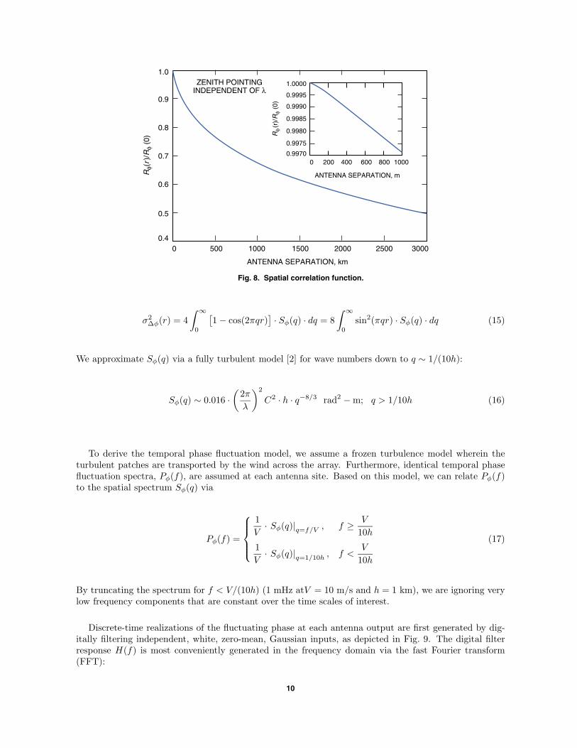
� (t) are guaranteed to have thecorrect temporal and spatial statistics. Sample realizations are depicted in Fig. 13, corresponding to thefollowing parameters:

N = 20 antennas

d = 500 m

frequency = 25 GHz (Ka-band)

vertical incidence, θ = 0 deg

Fs = 100 V/h = 1 Hz

turbulence parameters:

V = 10 m/s

h = 1 km

Γ = 3000 km

Fs = 100 V/h = 1 Hz

As is seen in Fig. 13, although the phase fluctuations apparently have an extremely high degree ofcorrelation, the corresponding phase difference data obey the modeled spatial structure function.

11

Fig. 10. Typical digital filter response: (a) frequency filter responsemagnitude and (b) filter impulse response.

0.2

0.00 5

f, mHz

10 15 20 25

0.4

0.6

0.8

1.0

V = 10 m/sh = 1 kmFs = 100 V/h = 1 Hz

f -4/3H

(f )

(a)

0.2

0.00

t, s

200 400

0.4

0.6

0.8

1.0

h (t

)

(b)

Fig. 11. Sample phase realization.

-1

0 500 1000 1500 2000

0

1

2

t, s

f (

t ), r

ad

INDEPENDENTPHASE

GENERATOR

Fig. 12. Generation of spatially correlated phaserealizations.

R

N (t )prop

N (t )

1 (t )prop

1 (t )

1 (t )prop

1 (t )prop

1 (t )propf

f

f

f

f

f

f

The computer model presented herein accurately models the phase structure function computed frompairs of elements. In particular it is shown that at the higher frequencies (25 GHz and above), significantcombining loss (0.5 dB or more) can occur for element baselines in excess of 300 m due to atmosphericturbulence. However, phase realizations generated by the computer model reveal that these effects occurat very low frequencies compared to the signal bandwidths of interest. Thus, they potentially can becompensated for via smart adaptive array processing. Nevertheless, these effects must be taken intoaccount in developing combining algorithms for large-array antennas.

IV. MUSIC Algorithm and Beam Forming

Spatially correlated interference poses challenges to the array-combining problem. To address the is-sues of identifying the intended and interference signals, and, furthermore, to suppress these interference

12

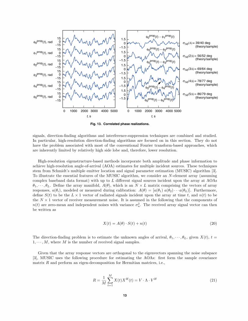
Fig. 13. Correlated phase realizations.

150

-15150

-15150

-15150

-15150

-15150

-15

0 1000 2000 3000 4000 5000

t, s

1.50

-1.5

1.50

-1.5

1.50

-1.5

1.50

-1.5

1.50

-1.5

0 1000 2000 3000 4000 5000

t, s

f0prop(t ) - f2

prop(t )

f0prop(t ) - f3

prop(t )

f0prop(t ) - f1

prop(t )

f0prop(t ) - f5

prop(t )

f0prop(t ) - f4

prop(t )

f0prop(t ), rad

f1prop(t ), rad

f2prop(t ), rad

f3prop(t ), rad

f4prop(t ), rad

f5prop(t ), rad

sDf(D) = 39/40 deg(theory/sample)

sDf(2D) = 56/52 deg(theory/sample)




signals, direction-finding algorithms and interference-suppression techniques are combined and studied.In particular, high-resolution direction-finding algorithms are focused on in this section. They do nothave the problem associated with most of the conventional Fourier transform-based approaches, whichare inherently limited by relatively high side lobe and, therefore, lower resolution.

High-resolution eigenstructure-based methods incorporate both amplitude and phase information toachieve high-resolution angle-of-arrival (AOA) estimates for multiple incident sources. These techniquesstem from Schmidt’s multiple emitter location and signal parameter estimation (MUSIC) algorithm [3].To illustrate the essential features of the MUSIC algorithm, we consider an N -element array (assumingcomplex baseband data format) with up to L different signal sources incident upon the array at AOAsθ1, · · · , θL. Define the array manifold, A(θ), which is an N × L matrix comprising the vectors of arrayresponses, a(θi), modeled or measured during calibration: A(θ) = [a(θ1) a(θ2) · · · a(θL)]. Furthermore,define S(t) to be the L × 1 vector of radiated signals incident upon the array at time t, and n(t) to bethe N × 1 vector of receiver measurement noise. It is assumed in the following that the components ofn(t) are zero-mean and independent noises with variance σ2

n. The received array signal vector can thenbe written as

X(t) = A(θ) · S(t) + n(t) (20)

The direction-finding problem is to estimate the unknown angles of arrival, θ1, · · · , θL, given X(t), t =1, · · · , M , where M is the number of received signal samples.

Given that the array response vectors are orthogonal to the eigenvectors spanning the noise subspace[3], MUSIC uses the following procedure for estimating the AOAs: first form the sample covariancematrix R and perform an eigen-decomposition for Hermitian matrices, i.e.,

R =1M

M∑t=1

X(t)XH(t) = V · Λ · V H (21)

13

where H denotes the conjugate transpose operation, Λ = diag(λ1, λ2, · · · , λN ), with the eigenvaluessatisfying λ1 ≥ λ2 ≥ · · · ≥ λN , and V = [ v1 v2 · · · vN ] are the corresponding orthonormal eigenvectorsof R. The unitary matrix of eigenvectors V can be decomposed further as V = [Vs Vn], where the columnsof Vs comprise the eigenvectors corresponding to the L largest eigenvalues of R (the signal subspace),and where Vn contains the remaining (noise) eigenvectors. Next the inverse MUSIC spectrum, F (θi), isformed via

F (θi) ≡1

‖V Hn · a(θi)‖2 (22)

Since the array response vectors a(θi) are orthogonal to the eigenvectors spanning the noise subspace Vn,it can be seen that the AOA estimates will occur at those θi’s that satisfy the equation

∥∥V Hn · a(θi)

∥∥2 = 0,

yielding the AOA estimate θ = arg maxθ1

{F (θi)}. The method can be readily extended to two-dimensionalarrays, as illustrated in the following.

As an example, Fig. 14 presents the results of applying MUSIC to a one-dimensional array configu-ration (10-element uniform linear array with half-wavelength spacing) with an incident signal and threeinterference plane wave components (to emulate planetary interference). The power in all signal andinterference components is assumed to be equal in this example, and the SNR per element is −15 dB.Figure 14(b) is the array response without adaptive interference cancellation. The three vertical straightlines indicate the location of the interfering sources. The MUSIC algorithm is first used to identifythe desired signal, impinging on axis, followed by identification of the three interference signals. Oncethese AOAs have been identified, an interference cancellation technique, such as the linear constrainedminimum-variance (LCMV) algorithm or the side lobe canceler, can be used to suppress the undesiredinterference sources. The antenna pattern presented in Fig. 14(a) is an example of the result from usingLCMV.

This approach can be further extended to form a continuous area of nulls in the spatial domain.In Fig. 15, a large planetary interference source has been modeled as a series of clustered distributedsources (again with the same power in the signal and interference components and approximately −15 dB

40

30

20

10

0-0.8-1.0

Fig. 14. MUSIC and adaptive cancellation: (a) with three-nullcancellation and (b) without cancellation.

GA

IN, d

B

u, sines

-0.6 -0.2-0.4 0.0 0.2 0.4 0.6 0.8 1.0

40

30

20

10

0

GA

IN, d

B

(b)

(a)

14

40

30

20

10

0-0.8-1.0

Fig. 15. MUSIC and zone cancellation: (a) with multiple-null (zone)cancellation and (b) without cancellation.

GA

IN, d

B

u, sines

-0.6 -0.2-0.4 0.0 0.2 0.4 0.6 0.8 1.0

40

30

20

10

0G

AIN

, dB

(b)

(a)

SNR per element). Provided the number of antenna elements in the array has a sufficient numberof degrees of freedom, typically on the order of 2 to 3 times that of the number of interferers, theadaptive cancellation technique, together with MUSIC, can be very effective for mitigating planetaryinterference. In such cases, large arrays can provide significant advantages over single-aperture antennasfor multibeam applications, such as improved SNR through suppression of planetary noise, together withrobust operation and improved availability.

When using the MUSIC algorithm, it is important to differentiate between the intended signal andspatially correlated interference signals. A JPL-developed generalized pre-processor algorithm [8,9] can beused to identify the intended signal and has been incorporated into the simulations. The concept presentedthere originated from the phase estimation problem under conditions of very low SNR characteristic ofdistant spacecraft, emergency-mode communications, and reception of turbo-coded signals where symbolSNRs of −6 dB are routinely encountered [10]. This technique also can provide significantly improvedphase estimates for the individual elements of a large antenna array.

As an example of operation with a 20-element linear array, Fig. 16 shows the MUSIC pseudo-spectrumof simulated spacecraft and planetary sources. Figure 17 shows the corresponding results after the pre-processor has been turned on. The incorporation of low SNR generalized pre-processor structures forcoded telemetry clearly enables greatly enhanced identification of spacecraft signals in the presence ofspatially overlapping interference when using the MUSIC algorithm.

The approach of combining high-resolution direction finding using MUSIC and interference cancellationusing beam forming can be extended from a one-dimensional to a two-dimensional planar array. Figure 18illustrates the two-dimensional inverse MUSIC spectrum of an 8-by-8 square planar array (half-wavelengthvertical and horizontal spacing between elements). The signal of interest arrives from (θ = 50 deg,φ = 0 deg), and the interfering signal arrives from (θ = 10 deg, φ = 0 deg), where θ is the angle fromthe normal to the array and φ is the corresponding azimuthal angle. These two signals are of equalpower (under noiseless conditions) and can be readily identified in the two-dimensional inverse MUSICspectrum. Figure 19 is a regional top view of the inverse spectrum where the two local peaks are clearlyformed at the two impinging directions.

15

20

15

10

5

0

-5

-10

-80 -60 -40 -20 0 20 40 60 80 100-100-15

25

MU

SIC

SP

EC

TR

UM

, dB

AOA, deg

DESIREDSPACECRAFTSIGNAL

INTERFERENCE

Fig. 16. Pseudo-spectrum of simulated spacecraftand planetary source.

10

5

0

-5

-10

-80 -60 -40 -20 0 20 40 60 80 100-100-15

15

MU

SIC

SP

EC

TR

UM

, dB

AOA, deg

DESIREDSPACECRAFTSIGNAL

Fig. 17. MUSIC plus pre-processor.

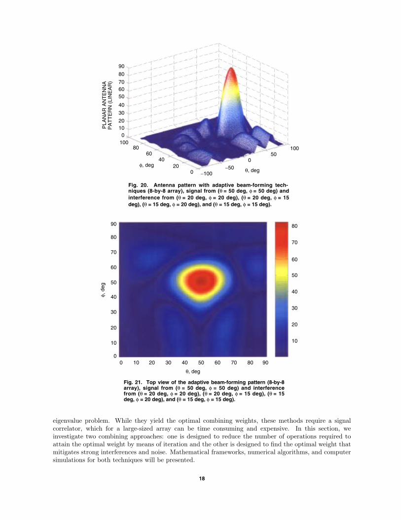
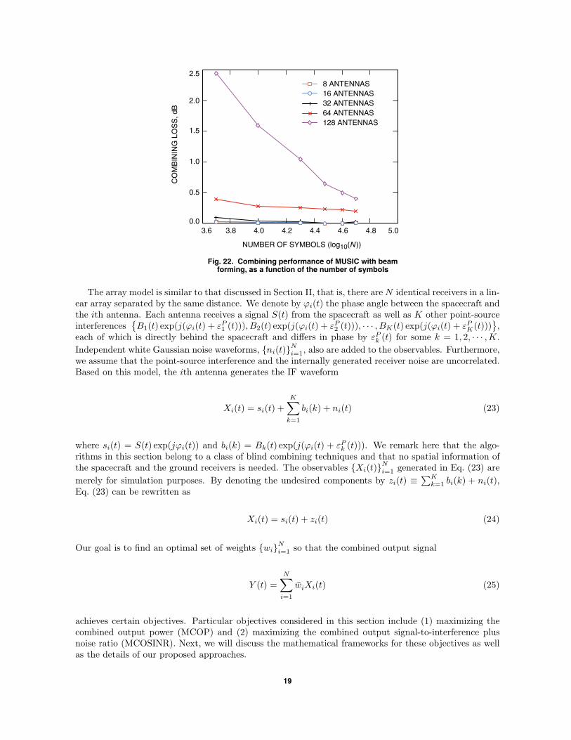
Given the angle of arrival estimates, two-dimensional adaptive beam-forming techniques can be carriedout to derive the optimum combining weights for the planar array. The two-dimensional antenna patternwith these weights is plotted in Fig. 20. In this example, the signal of interest comes from (θ = 50 deg,φ = 50 deg), and four interfering signals impinge from (θ = 20 deg, φ = 20 deg), (θ = 20 deg, φ = 15 deg),(θ = 15 deg, φ = 20 deg), and (θ = 15 deg, φ = 15 deg). The four point sources form a square, whichmodels a planar interfering source. The beam-forming algorithm is able to null out the interfering sources,as seen in Fig. 20 as well as in the regional top view of Fig. 21. The original beam pattern of the planararray is shaped to enhance the signal of interest while simultaneously nulling the interfering signals.

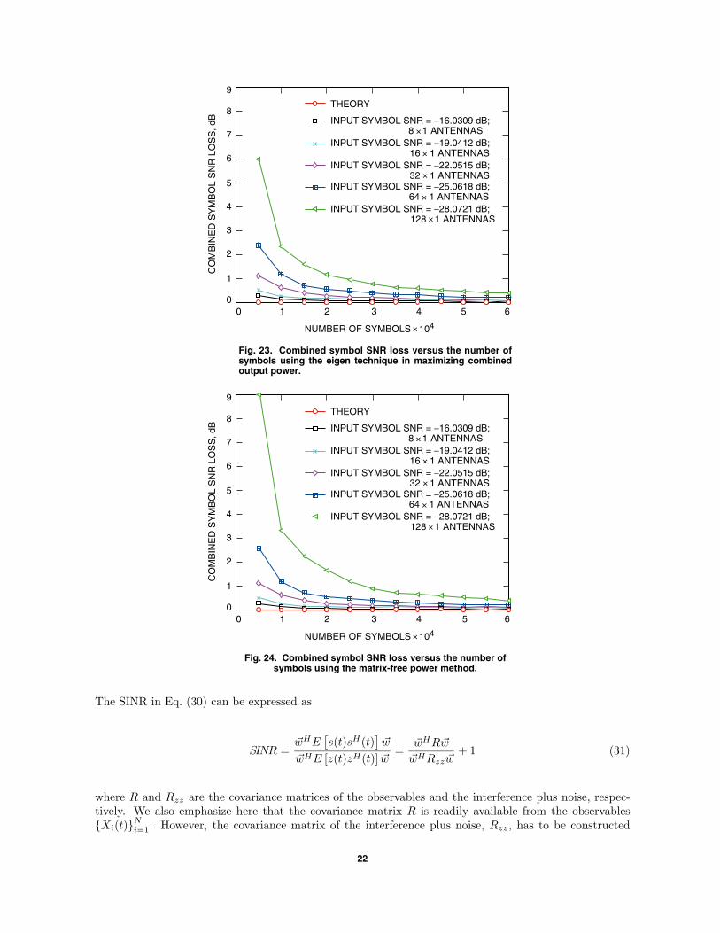
The communications performance of the MUSIC algorithm with beam forming can be assessed interms of the combining loss associated with the output signal of the array, that is, the loss comparedto a perfectly phased array of antennas. The results using this method are displayed in Fig. 22. Onlysignal plus receiver noise is considered in this example, with no additional interference signals. Thenumber of symbols within a block ranges from 5000 to 60,000 for each process. The combined outputsymbol SNR is fixed at −7 dB, and the received symbol SNR at each receiver is −(7+10 log10 N) dB. Thus,

16

-11

2-D

PS

EU

DO

-SP

EC

TR

UM

, dB

Fig. 18. 2-D MUSIC pseudo-spectrum (8-by-8 array), signal from(q = 50 deg, f = 0 deg) and the interfering signal from (q = 10deg, f = 0 deg).

10050

-50

-100 0

6080

100

f, deg

q, deg

-12

-13

-14

-15

-16

-17

-18

-19

4020

0

q, d

eg

Fig. 19. Regional top view of MUSIC pseudo-spectrum (8-by-8array), signal from (q = 50 deg, f = 0 deg) and the interfering sig-nal from (q = 10 deg, f = 0 deg).

90

80

70

60

50

40

30

20

10

00 10 20 30 40 50 60 70 80 90

-12

f, deg

-13

-14

-15

-16

-17

-18

the larger the array size, the smaller the received symbol SNR at each receiver. This accounts for therelatively large combining loss for the larger arrays. It can be seen that, when the number of symbolsexceeds 40,000 (where log10(40, 000) = 4.6), less than 0.5-dB combining loss can be achieved with arraysof 128 or fewer elements.

V. Eigen-Based Combining Algorithms

Traditional eigen-based combining algorithms (see a detailed survey in [4]) for large-array antennasrequire forming the covariance matrix of the observables between the array elements and solving an

17

90

PLA

NA

R A

NT

EN

NA

PA

TT

ER

N (

LIN

EA

R)

Fig. 20. Antenna pattern with adaptive beam-forming tech-niques (8-by-8 array), signal from (q = 50 deg, f = 50 deg) andinterference from (q = 20 deg, f = 20 deg), (q = 20 deg, f = 15deg), (q = 15 deg, f = 20 deg), and (q = 15 deg, f = 15 deg).

80

706050

40

30

2010

0100

8060

4020

0 -100-50

050

100

q, degf, deg

f, d

eg

Fig. 21. Top view of the adaptive beam-forming pattern (8-by-8array), signal from (q = 50 deg, f = 50 deg) and interferencefrom (q = 20 deg, f = 20 deg), (q = 20 deg, f = 15 deg), (q = 15deg, f = 20 deg), and (q = 15 deg, f = 15 deg).

90

80

70

60

50

40

30

20

10

00 10 20 30 40 50 60 70 80 90

80

70

60

50

40

30

20

10

q, deg

eigenvalue problem. While they yield the optimal combining weights, these methods require a signalcorrelator, which for a large-sized array can be time consuming and expensive. In this section, weinvestigate two combining approaches: one is designed to reduce the number of operations required toattain the optimal weight by means of iteration and the other is designed to find the optimal weight thatmitigates strong interferences and noise. Mathematical frameworks, numerical algorithms, and computersimulations for both techniques will be presented.

18

0.5

0.04.8 5.0

2.5

CO

MB

ININ

G L

OS

S, d

B

NUMBER OF SYMBOLS (log10(N ))

Fig. 22. Combining performance of MUSIC with beamforming, as a function of the number of symbols

8 ANTENNAS16 ANTENNAS32 ANTENNAS64 ANTENNAS128 ANTENNAS

1.0

1.5

2.0

4.64.44.24.03.83.6

The array model is similar to that discussed in Section II, that is, there are N identical receivers in a lin-ear array separated by the same distance. We denote by ϕi(t) the phase angle between the spacecraft andthe ith antenna. Each antenna receives a signal S(t) from the spacecraft as well as K other point-sourceinterferences

{B1(t) exp(j(ϕi(t) + εP

1 (t))), B2(t) exp(j(ϕi(t) + εP2 (t))), · · · , BK(t) exp(j(ϕi(t) + εP

K(t)))},

each of which is directly behind the spacecraft and differs in phase by εPk (t) for some k = 1, 2, · · · , K.

Independent white Gaussian noise waveforms, {ni(t)}Ni=1, also are added to the observables. Furthermore,

we assume that the point-source interference and the internally generated receiver noise are uncorrelated.Based on this model, the ith antenna generates the IF waveform

Xi(t) = si(t) +K∑

k=1

bi(k) + ni(t) (23)

where si(t) = S(t) exp(jϕi(t)) and bi(k) = Bk(t) exp(j(ϕi(t) + εPk (t))). We remark here that the algo-

rithms in this section belong to a class of blind combining techniques and that no spatial information ofthe spacecraft and the ground receivers is needed. The observables {Xi(t)}N

i=1 generated in Eq. (23) aremerely for simulation purposes. By denoting the undesired components by zi(t) ≡

∑Kk=1 bi(k) + ni(t),

Eq. (23) can be rewritten as

Xi(t) = si(t) + zi(t) (24)

Our goal is to find an optimal set of weights {wi}Ni=1 so that the combined output signal

Y (t) =N∑

i=1

wiXi(t) (25)

achieves certain objectives. Particular objectives considered in this section include (1) maximizing thecombined output power (MCOP) and (2) maximizing the combined output signal-to-interference plusnoise ratio (MCOSINR). Next, we will discuss the mathematical frameworks for these objectives as wellas the details of our proposed approaches.

19

A. Maximizing the Combined Output Power (MCOP)

As its name indicates, the MCOP algorithm is designed to find a normalized set of weight thatmaximizes the combined time-average output signal power, which we define as E[||Y (t)||2], where E[·]again denotes the time-average expected value operator. It can be shown easily that the combined outputsignal power can be expressed in the quadratic form of the covariance matrix, i.e.,

E[||Y (t)||2] = E

[∣∣∣∣∣∣∣∣

N∑i=1

wiXi(t)∣∣∣∣∣∣∣∣2]

= wH

(1M

M∑m=1

Xi(m)XHi

(m)

) w = wHR w (26)

Taking advantage of the eigen decomposition of the covariance matrix R defined in Eq. (21), any arbitraryset of unit weight w can be written as

w =N∑

i=1

αi vi = V α (27)

where α = [α1, α2, · · · , αN ]T and∑N

i=1 |αi|2 = 1.

Putting the combined output power, Eq. (26), in normalized form, we have

E[∣∣∣∣Y (t)

∣∣∣∣2] = (V α)HV ΛV H(V α) = αHΛ α =N∑

i=1

λi|αi|2 ≤ λ1 (28)

Therefore, the weight that yields the largest combined output power is the eigenvector that corresponds tothe largest eigenvalue. Traditional procedures for finding the dominant eigenvector include the following:

(1) Form the covariance matrix R.

(2) Solve the eigen problem R v = λ v and sort the eigenvalues λ1 ≥ λ2 ≥ · · · ≥ λN .

(3) Set wopt = v1.

Note that the above approach solves for all eigenvectors, while it uses only the dominant one. Therefore,a more efficient technique is needed, which turns out to be a well-known numerical algorithm calledthe power method [5]. The power method finds iteratively and solely the dominant eigenvector and isimplemented as follows:

(1) Form the covariance matrix R.

(2) Start with w(0) = [1, · · · , 1]T /√

N and compute successively w(k) = R w(k−1)/||R w(k−1)||.(3) Set wopt = w(k).

Note that while it eliminates many of the unnecessary computations of non-dominant eigenvectors, thepower method requires the formation of the covariance matrix R. As a result, the total number of floating-point operations is N(N + 1)M/2 + N2I, where again N is the number of antennas, M is the number ofsignal samples within a received block, and I is the number of iterations. To reduce further the numberof floating-point operations and to remove the requirement for forming the covariance matrix, we proposethe following algorithm, which we call the matrix-free power method:

20

(1) Start with an initial guess w(0) = [1, · · · , 1]T /√

N .

(2) Compute successively w(k) = u(k)/|| u(k)||, where

u(k)j = E

[Xj(t)Y (t)

]

Y (t) =N∑

i=1

w(k−1)i Xi(t)

(29)

(3) Set wopt = w(k).

With simple algebraic manipulations, one can see that u(k)j in Eq. (29) is exactly R w(k−1). The number

of floating-point operations is reduced to N · M · I. The convergence of the power method is dictatedby the separation of the signal power to the noise power and the number of iterations is bounded, in theworst-case scenario, by N . Moreover, the number of iterations may be large for the first block of symbols,but, in most cases, I << N, M .

Since the MCOP approach maximizes the combined output power, when undesired signals are presentand are as strong as the desired signal, the MCOP approach amplifies both the desired and undesiredsignals. It appears that this approach is most suitable when there are no interfering sources present. In ourfirst simulations, we assume that the observables consist of only signal plus internally generated receivernoise and that there are no interfering sources from nearby planets. In fact, this particular approachhas been studied by Hackett [6], where he proposed this technique as a means to adaptively separatethe communications signals in an antenna array. He found the optimal weight by forming the covariancematrix of the observables and used the standard eigen technique to find the dominant eigenvector.

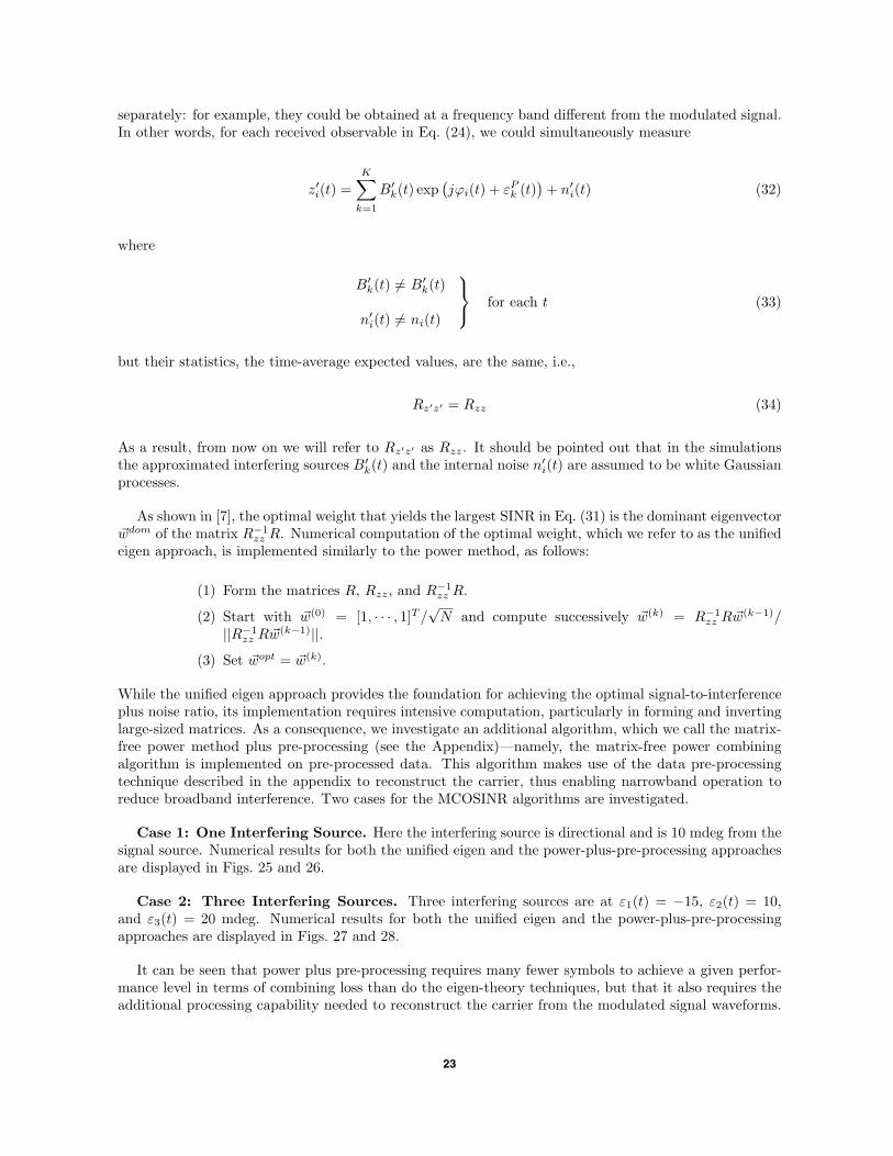
In our simulations, we assume that the antennas are 20 m apart and the thermal noise at each receiveris broadband. The combined output symbol SNR is fixed at −7 dB, and the received symbol SNR ateach receiver is −(7 + 10 log10 N) dB. The number of symbols within a block ranges from 5000 to 60,000,as in the MUSIC approach discussed in Section IV. The results using the traditional eigen method aredisplayed in Fig. 23.

We find that the eigen-based combining technique can successfully increase the output SNR and that,if the input symbol SNR is small, the number of symbols within a processing block must be sufficientlylarge to avoid severe combined symbol SNR degradation. To justify numerically the proposed matrix-freepower method, the same scenario as that used for the traditional eigen method is simulated, with theresults depicted in Fig. 24. Here the loss fluctuates slightly for a small input symbol SNR and a smallnumber of symbols per processing block. As expected, the combined symbol SNR for the traditional eigenand the matrix-free power methods compare well when the number of symbols exceeds 50,000.

B. Maximizing the Combined Output Signal-to-Interference Plus Noise Ratio (MCOSINR)

The second approach (MCOSINR) is designed to maximize the combined output signal-to-interferenceplus noise ratio (SINR), which we define as

SINR =E

[∣∣∣∣∣∣ N∑i=1

wisi(t)∣∣∣∣∣∣]2

E

[∣∣∣∣∣∣ N∑i=1

wizi(t)∣∣∣∣∣∣2] (30)

21

INPUT SYMBOL SNR = -16.0309 dB;8 1 ANTENNAS

2

05 6

CO

MB

INE

D S

YM

BO

L S

NR

LO

SS

, dB

NUMBER OF SYMBOLS 104

Fig. 23. Combined symbol SNR loss versus the number ofsymbols using the eigen technique in maximizing combinedoutput power.

3

7

8

43210





9

6

5

4

1

THEORY


2

05 6

CO

MB

INE

D S

YM

BO

L S

NR

LO

SS

, dB


Fig. 24. Combined symbol SNR loss versus the number ofsymbols using the matrix-free power method.

3

7

8

43210





9

6

5

4

1

THEORY

The SINR in Eq. (30) can be expressed as

SINR = wHE

[s(t)sH(t)

] w

wHE [z(t)zH(t)] w=

wHR w

wHRzz w+ 1 (31)

where R and Rzz are the covariance matrices of the observables and the interference plus noise, respec-tively. We also emphasize here that the covariance matrix R is readily available from the observables{Xi(t)}N

i=1. However, the covariance matrix of the interference plus noise, Rzz, has to be constructed

22

separately: for example, they could be obtained at a frequency band different from the modulated signal.In other words, for each received observable in Eq. (24), we could simultaneously measure

z′i(t) =K∑

k=1

B′k(t) exp

(jϕi(t) + εP

k (t))

+ n′i(t) (32)

where

B′k(t) = B′

k(t)

n′i(t) = ni(t)

for each t (33)

but their statistics, the time-average expected values, are the same, i.e.,

Rz′z′ = Rzz (34)

As a result, from now on we will refer to Rz′z′ as Rzz. It should be pointed out that in the simulationsthe approximated interfering sources B′

k(t) and the internal noise n′i(t) are assumed to be white Gaussian

processes.

As shown in [7], the optimal weight that yields the largest SINR in Eq. (31) is the dominant eigenvector wdom of the matrix R−1

zz R. Numerical computation of the optimal weight, which we refer to as the unifiedeigen approach, is implemented similarly to the power method, as follows:

(1) Form the matrices R, Rzz, and R−1zz R.

(2) Start with w(0) = [1, · · · , 1]T /√

N and compute successively w(k) = R−1zz R w(k−1)/

||R−1zz R w(k−1)||.

(3) Set wopt = w(k).

While the unified eigen approach provides the foundation for achieving the optimal signal-to-interferenceplus noise ratio, its implementation requires intensive computation, particularly in forming and invertinglarge-sized matrices. As a consequence, we investigate an additional algorithm, which we call the matrix-free power method plus pre-processing (see the Appendix)—namely, the matrix-free power combiningalgorithm is implemented on pre-processed data. This algorithm makes use of the data pre-processingtechnique described in the appendix to reconstruct the carrier, thus enabling narrowband operation toreduce broadband interference. Two cases for the MCOSINR algorithms are investigated.

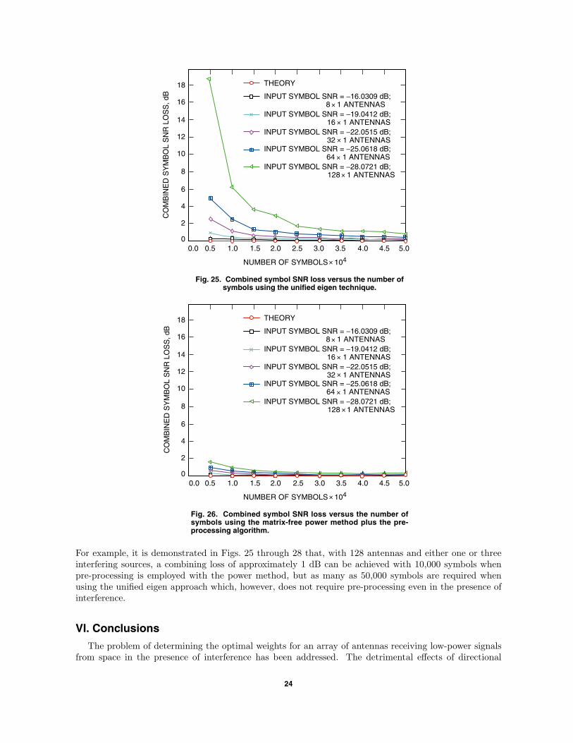
Case 1: One Interfering Source. Here the interfering source is directional and is 10 mdeg from thesignal source. Numerical results for both the unified eigen and the power-plus-pre-processing approachesare displayed in Figs. 25 and 26.

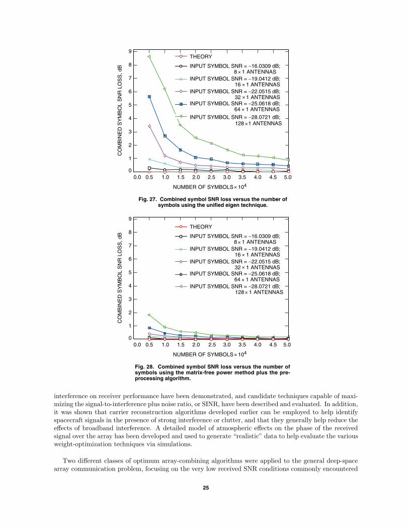
Case 2: Three Interfering Sources. Three interfering sources are at ε1(t) = −15, ε2(t) = 10,and ε3(t) = 20 mdeg. Numerical results for both the unified eigen and the power-plus-pre-processingapproaches are displayed in Figs. 27 and 28.

It can be seen that power plus pre-processing requires many fewer symbols to achieve a given perfor-mance level in terms of combining loss than do the eigen-theory techniques, but that it also requires theadditional processing capability needed to reconstruct the carrier from the modulated signal waveforms.

23


4

04.0 5.0

CO

MB

INE

D S

YM

BO

L S

NR

LO

SS

, dB


Fig. 25. Combined symbol SNR loss versus the number ofsymbols using the unified eigen technique.

8

16

18

3.02.01.50.50.0





14

12

10

2

THEORY

6

1.0 2.5 3.5 4.5


4

04.0 5.0

CO

MB

INE

D S

YM

BO

L S

NR

LO

SS

, dB


Fig. 26. Combined symbol SNR loss versus the number ofsymbols using the matrix-free power method plus the pre-processing algorithm.

8

16

18

3.02.01.50.50.0





14

12

10

2

THEORY

6

1.0 2.5 3.5 4.5

For example, it is demonstrated in Figs. 25 through 28 that, with 128 antennas and either one or threeinterfering sources, a combining loss of approximately 1 dB can be achieved with 10,000 symbols whenpre-processing is employed with the power method, but as many as 50,000 symbols are required whenusing the unified eigen approach which, however, does not require pre-processing even in the presence ofinterference.

VI. Conclusions

The problem of determining the optimal weights for an array of antennas receiving low-power signalsfrom space in the presence of interference has been addressed. The detrimental effects of directional

24

3.52.5 4.5


2

04.0 5.0

CO

MB

INE

D S

YM

BO

L S

NR

LO

SS

, dB


Fig. 27. Combined symbol SNR loss versus the number ofsymbols using the unified eigen technique.

4

8

9

3.02.01.50.50.0





7

6

5

1

THEORY

3

1.0

3.52.5 4.5






THEORY

2

04.0 5.0

CO

MB

INE

D S

YM

BO

L S

NR

LO

SS

, dB


Fig. 28. Combined symbol SNR loss versus the number ofsymbols using the matrix-free power method plus the pre-processing algorithm.

4

8

9

3.02.01.50.50.0

7

6

5

1

3

1.0

interference on receiver performance have been demonstrated, and candidate techniques capable of maxi-mizing the signal-to-interference plus noise ratio, or SINR, have been described and evaluated. In addition,it was shown that carrier reconstruction algorithms developed earlier can be employed to help identifyspacecraft signals in the presence of strong interference or clutter, and that they generally help reduce theeffects of broadband interference. A detailed model of atmospheric effects on the phase of the receivedsignal over the array has been developed and used to generate “realistic” data to help evaluate the variousweight-optimization techniques via simulations.

Two different classes of optimum array-combining algorithms were applied to the general deep-spacearray communication problem, focusing on the very low received SNR conditions commonly encountered

25

over the deep-space channel. It was shown that both the subspace-based MUSIC algorithm and theclass of eigen-theory algorithms are strong candidates for this application, with capabilities that providefor signal and interference identification as well as interference suppression to maximize the combinedsignal-to-noise ratio.

References

[1] T. Cwik, V. Jamnejad, and G. Resch, A Study of the Synthesis of a LargeCommunications Aperture Using Small Antennas, JPL Publication 93-1497, JetPropulsion Laboratory, Pasadena, California, September 22, 1993.

[2] A. R. Thompson, J. Moran, and G. Swenson, Interferometry and Synthesis inRadio Astronomy, New York: Wiley, 1986.

[3] R. Schmidt, “Multiple Emitter Location and Signal Parameter Estimation,” Pro-ceedings RADC Spectrum Estimation Workshop, Griffiths Air Force Base, NewYork, pp. 243–258, 1979; also in IEEE Trans. Antennas Prop., vol. AP-34, no. 3,pp. 276–280, March 1986.

[4] L. C. Godara, “Application of Antenna Arrays to Mobile Communications.II. Beam-Forming and Direction-of-Arrival Considerations,” Proceedings of theIEEE, vol. 85, issue 8, pp. 1195–1245, August 1997.

[5] C. A. Hall and T. A. Porsching “Computing the Maximal Eigenvalue and Eigen-vector,” SIAM J. Numer. Analysis, vol. 5, N2, pp. 269–274, 1968.

[6] C. M. Hackett, Jr., “ Adaptive Arrays Can be Used to Separate CommunicationSignals,” IEEE Transactions on Aerospace and Electronic Systems, vol. AES-17,no. 2, pp. 234–247, March 1981.

[7] K.-M. Cheung, “Eigen Theory for Optimal Signal Combining: A Unified Ap-proach,” The Telecommunications and Data Acquisition Progress Report 42-126,April–June 1996, Jet Propulsion Laboratory, Pasadena, California, pp. 1–9, Au-gust 15, 1996.http://tmo.jpl.nasa.gov/tmo/progress report/42-126/126C.pdf

[8] M. K. Simon and V. A. Vilnrotter, “Iterative Information-Reduced Carrier Syn-chronization Using Decision Feedback for Low SNR Applications,” The Telecom-munications and Data Acquisition Progress Report 42-130, April–June 1997, JetPropulsion Laboratory, Pasadena, California, pp. 1–21, August 15, 1997.http://tmo.jpl.nasa.gov/tmo/progress report/42-130/130A.pdf

[9] V. Vilnrotter, A. Gray, and C. Lee “Carrier Synchronization for Low Signal-to-Noise Ratio Binary Phase-Shift-Keyed Modulated Signals,” The Telecommuni-cations and Mission Operations Progress Report 42-139, July–September 1999,Jet Propulsion Laboratory, Pasadena, California, pp. 1–16, November 15, 1999.http://tmo.jpl.nasa.gov/tmo/progress report/42-139/139I.pdf

[10] V. Vilnrotter, C. Lee, and N. Lay “A Generalized Pre-Processor for Block andConvolutionally Coded Signals,” The Telecommunications and Mission Opera-tions Progress Report 42-144, October–December 2000, Jet Propulsion Labora-tory, Pasadena, California, pp. 1–19, February 15, 2001.http://tmo.jpl.nasa.gov/tmo/progress report/42-144/144G.pdf

26

Appendix

Generalized Pre-Processor

The use of data pre-processors for reconstructing the carrier from binary-phase shift keyed (BPSK)-modulated block and convolutionally coded signals has been described in previous articles [8,9]. Thebasic system concept is as follows: The data sequence first is estimated using a data pre-processor, afterwhich the estimated data sequence is multiplied by a delayed version of the sampled waveform. Evenif the data estimates contain some errors, the original data modulation will be largely removed, leavingonly a residual error sequence on the carrier with a necessarily lower transition rate than the originalsignal; therefore, this partially reconstructed carrier typically occupies a much narrower bandwidth thandoes the original data modulation.

A maximum-likelihood block-decision approach for block-encoded sequences of BPSK symbols hasbeen described in [10], where it was demonstrated that this approach also can be applied to convolutionalcodes, enabling the generalization of the pre-processor structure to most encoding schemes employedor contemplated by the DSN, including turbo codes. Two block-decoding schemes for convolutionallyencoded data have been simulated. First, decoder performance was bounded by assuming that the stateof the registers is known after each input block. This is a useful bound, but not a practical decodingscheme because in reality the states are not known, and hence must be estimated along with the code-words. Incorrect decoding results in loss of state information, which means the pre-processor generatesthe wrong codeword set for correlation with the received signal. This, in turn, leads to incorrect decodingof subsequent codewords, with little chance of ever recovering the correct state. This lower bound onpre-processor symbol-error rate is illustrated in Fig. A-1 by the curve labeled “pre-processor (known statebound)” and represents a performance bound that is generally not attainable in practice. The secondscheme makes no attempt to estimate the state of the encoder; hence, the pre-processor must correlatethe received waveform with all possible codewords associated with every state. Symbol-error performancefor this approach is also shown in Fig. A-1 as the curve labeled “pre-processor (all states).” Its symbol-error performance is approximately 1.5-dB worse than that of the known-states bound. Finally, the

0.00-2 0

SY

MB

OL

ER

RO

R P

RO

BA

BIL

ITY

P (

SE

)

ES /N0, dB

Fig. A-1. Probability of binary symbol error for convolution-ally coded symbols, block-length-8 decoding. The perfor-mance of the Viterbi decoder on the same sequence is alsoincluded for reference.

0.35

0.40

-4-6-10 -8

PRE-PROCESSOR(KNOWN STATE BOUND)

VITERBIDECODER

PRE-PROCESSOR(ALL STATES)

ALL POSSIBLESEQUENCES

0.30

0.25

0.20

0.15

0.10

0.05

27

symbol-error performance of a conventional Viterbi decoder of the type generally used in the DSN alsohas been included for comparison, labeled “Viterbi decoder” in Fig. A-1. In order to evaluate the Viterbidecoder in the same framework as the pre-processor, it was operated with a fixed delay of 8 symbols.Symbol-error performance of the Viterbi decoder operated in this mode is seen to be worse than that ofthe block pre-processor at SNRs less than −4 dB. Thus, when channel dynamics dictate operation withrelatively short delays, the block pre-processor appears to have a clear advantage over the conventionalViterbi decoder in the region of very low signal-to-noise ratios.

28

Documents

Large-Array Signal Processing for Deep-Space Applications