Embed Size (px)
Citation preview
Lappeenranta University of Technology
LUT School of Energy Systems
LUT Mechanical Engineering
Shayan Moradkhani
VIRTUAL REALITY SIMULATION FOR THE CONDITION MONITORING OF
ROBOT IN FUSION REACTOR APPLICATION
Examiners: Adjunct professor Huapeng Wu
Professor Heikki Handroos
ABSTRACT
Lappeenranta University of Technology
LUT School of Energy Systems
LUT Mechanical Engineering
Shayan Moradkhani
Virtual reality simulation for the condition monitoring of robot in fusion reactor
application
Master’s thesis
2018
54 pages, 28 figures
Examiners: Adjunct professor Huapeng Wu
Professor Heikki Handroos
Keywords: Parallel manipulator, real-time simulation, PLC TwinCat 3
This thesis aims to prepare a 3D simulation environment for the robot in order to be controlled by
a PLC TwinCat3. For that a comparison between different 3D simulation environments is made,
which could communicate with PLC in real-time. The robot model is taken from a previous
master’s thesis carried out by Chanyang Li and the robot model components were designed in
SolidWorks. The model components are exported individually and assemble in the new
environment. The mathematical model of the robot is derived using inverse kinematics and the
offline simulation in the Unreal Engine (UE) approves the equations. Then using the server-client
scenario, a PLC module is created in C++ as the server, and a client module is set up in the UE in
C++ structure. Then the real-time communication between PLC and UE is stablished and the input
variables for the inverse kinematics of the parallel manipulator is provided with the PLC.

ACKNOWLEDGEMENTS
I want to express my appreciation for the support and supervision I was provided by Professor
Huapeng Wu as my supervisor.
Special thanks to my family and my friends who have been supportive emotionally throughout the
whole process of this thesis work.
4
TABLE OF CONTENTS
ABSTRACT .................................................................................................................................... 2
ACKNOWLEDGEMENTS ............................................................................................................ 3
Table of contents ............................................................................................................................. 4
Table of figures ............................................................................................................................... 6
LIST OF SUMBOLS AND ABBREVIATIONS ........................................................................... 8
1. Introduction ............................................................................................................................. 9
1.1. Robot description .......................................................................................................... 10
1.2. Robotic simulation ........................................................................................................ 15
1.3. Computer graphics ........................................................................................................ 15
1.4. Simulation environment options ................................................................................... 16
1.4.1. OpenGL................................................................................................................... 16
1.4.2. Direct3D .................................................................................................................. 18
1.4.3. VTK ........................................................................................................................ 21
1.4.4. Unity3D................................................................................................................... 22
1.4.5. SimMechanics ......................................................................................................... 24
1.4.6. ROS ......................................................................................................................... 27
1.4.7. Adams ..................................................................................................................... 29
1.4.8. Unreal Engine ......................................................................................................... 30
1.5. PLC ............................................................................................................................... 33
2. Thesis objective and motivation ........................................................................................... 37
3. Methodology ......................................................................................................................... 41
4. Results ................................................................................................................................... 49
5. Discussion ............................................................................................................................. 50

5
6. Conclusion ............................................................................................................................ 51
References ..................................................................................................................................... 52
6
TABLE OF FIGURES
Figure 1. Schematic of the vacuum vessel of the fusion reactor, inside which the IWR is
implemented [1] ............................................................................................................................ 10
Figure 2. parallel robot used in this study for simulation[2]. ........................................................ 10
Figure 3. 3D view of the carriage for the parallel robot[2]. .......................................................... 11
Figure 4. the 3D schematic of the frame designed for the parallel robot[2]. ................................ 11
Figure 5. parallel manipulator used in the studied robot[2]. ......................................................... 12
Figure 6. Hexapod parallel mechanism[6]. ................................................................................... 13
Figure 7.the circle containing the joint positions is parallel with highlighted surface of the frame
is [2]. ............................................................................................................................................. 14
Figure 8. 3D model of the end-effector shown with red arrow [2] ............................................... 14
Figure 9. buffer swap during the animation [10]. ......................................................................... 20
Figure 10. Unity3D game architecture using components [17]. ................................................... 23
Figure 11. Unity3D general class categorization [17]. ................................................................. 23
Figure 12. schematic of inverted double pendulum [18]. ............................................................. 25
Figure 13. Simulink model of the inverted double pendulum using SimMechanics [18]. ........... 26
Figure 14. schematic of node implementation in a custom ROS application [21]. ...................... 27
Figure 15. Graph structure in ROS utilizing topics, nodes, and services [20]. ............................. 29
Figure 16. ITER vacuum vessel schematic with the track rail and the parallel manipulator [1] .. 37
Figure 17. Close-up section of the ITER vacuum vessel with end-effector path and robot placement
with respect to the track rail [1]. ................................................................................................... 38
Figure 18. Status of the parallel manipulator test bench in the LUT laboratory .......................... 38
Figure 19. Milling and welding tools mounted on the changeable interface of the end-effector . 39
Figure 20. IWR real-time operation scenario ............................................................................... 40
Figure 21. Stewart platform, parallel manipulator consisting of 6 actuator [30] .......................... 43
Figure 22. Calculation of the actuator vectors using blueprints in UE ......................................... 44
Figure 23. First raw of the rotation matrix in UE using BP .......................................................... 45
Figure 24. The final assembly of the robot CAD files, imported into UE from SolidWorks ....... 45
Figure 25. End-effector position vector; red for x, green for y, and blue for z values ................. 46

7
Figure 26. End-effector orientation vectors; red for alpha, green for beta, and blue for Gama ... 46
Figure 27. General scenario for the collision concept in robotics applications [31] .................... 47
Figure 28. Lack of movement limitation on the pistons resulted in an abnormal actuators
configuration. ................................................................................................................................ 49
8
LIST OF SUMBOLS AND ABBREVIATIONS
ADS Automation Device Specification
AI Artificial Intelligence
API Application Programming Interface
BP Blueprint
CAD Computer Aided Design
COM Component Object Model
CPU Central Processing Unit
DOF Degrees Of Freedom
GUI Graphical User Interface
GPU Graphical Processing Unit
HMI Human Machine Interface
ITER International Thermonuclear Experimental Reactor
IWR Intersector Welding Robot
LUT Lappeenranta University of Technology
MBD Multi-Body Dynamics
NDT Non-Destructive Testing
RGB Red Green Blue
ROS Robotics Operating System
TCP Transmission Control Protocol)
UDP User Datagram Protocol)
VBO Vertex Buffer Object
VTK Visualization Tool-Kit
VTT Technical Research Center of Finland
9
1. INTRODUCTION
Combination of technology and engineering management systems enable operators to safely,
reliably and repeatedly perform manipulation of items, in environments, which are harsh for
humans, without being in personal contact with those items [1]. In order to achieve that, one should
be able to simulate the mechanisms in real-time to predict the actual motion and any potential
collision between the parts. The closer simulation of the mechanism to the actual laboratory
condition, the more reliable is the condition monitoring and motion prediction as it ensures the
safety of the robot operation inside of the fusion reactor. In order to achieve this objective, one
should have good grasp of, the implemented mechanical system or robot, simulation environments
and how they work, and the real-time communication with other platforms.
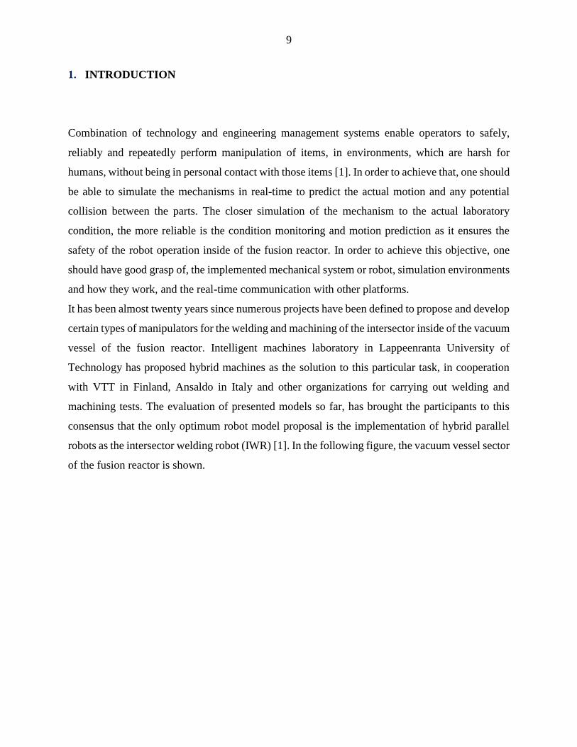
It has been almost twenty years since numerous projects have been defined to propose and develop
certain types of manipulators for the welding and machining of the intersector inside of the vacuum
vessel of the fusion reactor. Intelligent machines laboratory in Lappeenranta University of
Technology has proposed hybrid machines as the solution to this particular task, in cooperation
with VTT in Finland, Ansaldo in Italy and other organizations for carrying out welding and
machining tests. The evaluation of presented models so far, has brought the participants to this
consensus that the only optimum robot model proposal is the implementation of hybrid parallel
robots as the intersector welding robot (IWR) [1]. In the following figure, the vacuum vessel sector
of the fusion reactor is shown.
10
Figure 1. Schematic of the vacuum vessel of the fusion reactor, inside which the IWR is
implemented [1].
1.1. Robot description
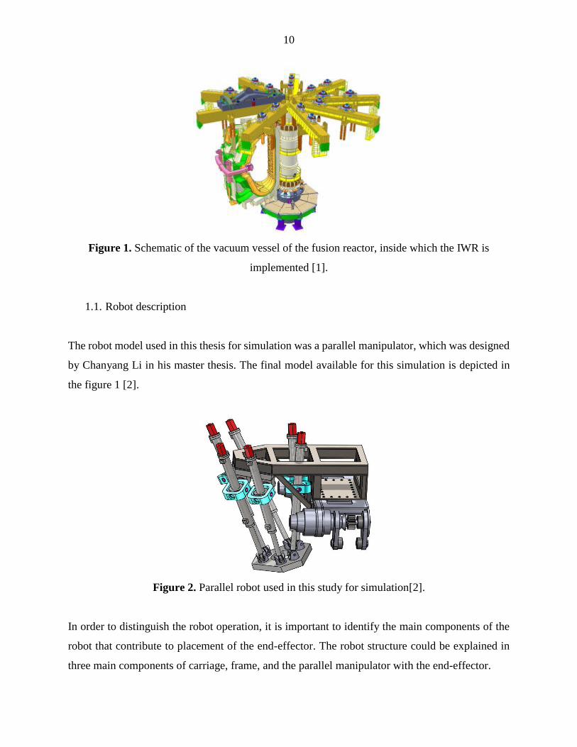
The robot model used in this thesis for simulation was a parallel manipulator, which was designed
by Chanyang Li in his master thesis. The final model available for this simulation is depicted in
the figure 1 [2].
Figure 2. Parallel robot used in this study for simulation[2].
In order to distinguish the robot operation, it is important to identify the main components of the
robot that contribute to placement of the end-effector. The robot structure could be explained in
three main components of carriage, frame, and the parallel manipulator with the end-effector.
11
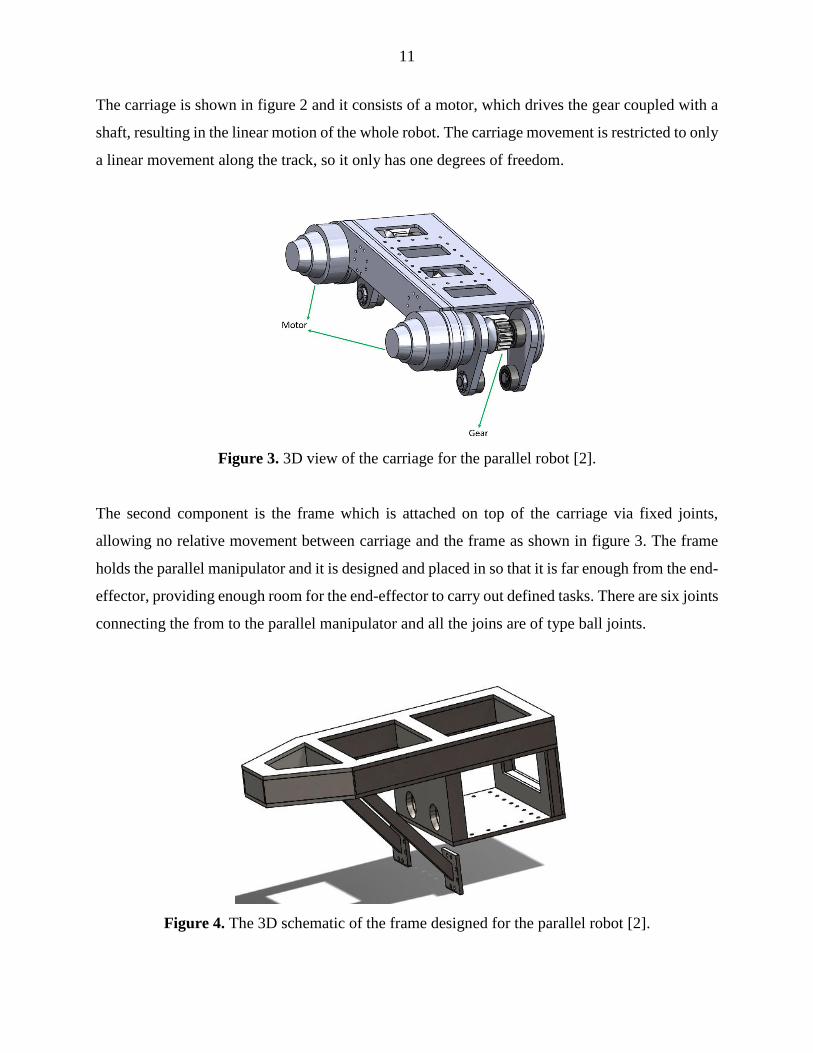
The carriage is shown in figure 2 and it consists of a motor, which drives the gear coupled with a
shaft, resulting in the linear motion of the whole robot. The carriage movement is restricted to only
a linear movement along the track, so it only has one degrees of freedom.
Figure 3. 3D view of the carriage for the parallel robot [2].
The second component is the frame which is attached on top of the carriage via fixed joints,
allowing no relative movement between carriage and the frame as shown in figure 3. The frame
holds the parallel manipulator and it is designed and placed in so that it is far enough from the end-
effector, providing enough room for the end-effector to carry out defined tasks. There are six joints
connecting the from to the parallel manipulator and all the joins are of type ball joints.
Figure 4. The 3D schematic of the frame designed for the parallel robot [2].
12
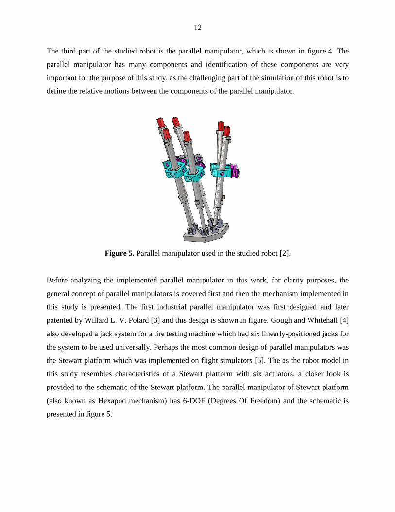
The third part of the studied robot is the parallel manipulator, which is shown in figure 4. The
parallel manipulator has many components and identification of these components are very
important for the purpose of this study, as the challenging part of the simulation of this robot is to
define the relative motions between the components of the parallel manipulator.
Figure 5. Parallel manipulator used in the studied robot [2].
Before analyzing the implemented parallel manipulator in this work, for clarity purposes, the
general concept of parallel manipulators is covered first and then the mechanism implemented in
this study is presented. The first industrial parallel manipulator was first designed and later
patented by Willard L. V. Polard [3] and this design is shown in figure. Gough and Whitehall [4]
also developed a jack system for a tire testing machine which had six linearly-positioned jacks for
the system to be used universally. Perhaps the most common design of parallel manipulators was
the Stewart platform which was implemented on flight simulators [5]. The as the robot model in
this study resembles characteristics of a Stewart platform with six actuators, a closer look is
provided to the schematic of the Stewart platform. The parallel manipulator of Stewart platform
(also known as Hexapod mechanism) has 6-DOF (Degrees Of Freedom) and the schematic is
presented in figure 5.
13
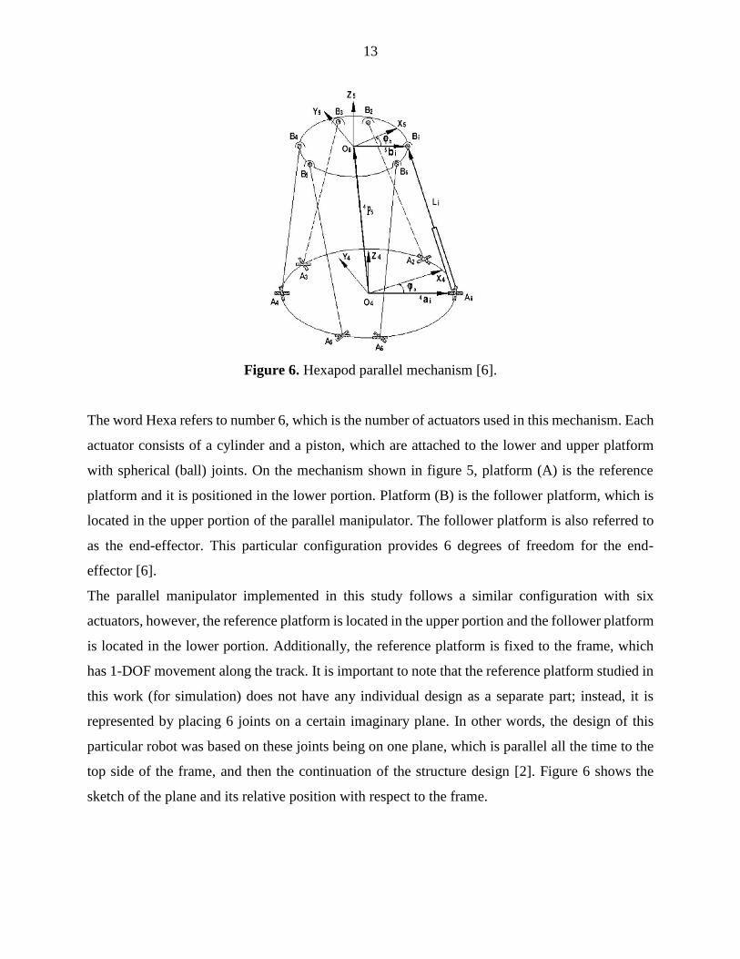
Figure 6. Hexapod parallel mechanism [6].
The word Hexa refers to number 6, which is the number of actuators used in this mechanism. Each
actuator consists of a cylinder and a piston, which are attached to the lower and upper platform
with spherical (ball) joints. On the mechanism shown in figure 5, platform (A) is the reference
platform and it is positioned in the lower portion. Platform (B) is the follower platform, which is
located in the upper portion of the parallel manipulator. The follower platform is also referred to
as the end-effector. This particular configuration provides 6 degrees of freedom for the end-
effector [6].
The parallel manipulator implemented in this study follows a similar configuration with six
actuators, however, the reference platform is located in the upper portion and the follower platform
is located in the lower portion. Additionally, the reference platform is fixed to the frame, which
has 1-DOF movement along the track. It is important to note that the reference platform studied in
this work (for simulation) does not have any individual design as a separate part; instead, it is
represented by placing 6 joints on a certain imaginary plane. In other words, the design of this
particular robot was based on these joints being on one plane, which is parallel all the time to the
top side of the frame, and then the continuation of the structure design [2]. Figure 6 shows the
sketch of the plane and its relative position with respect to the frame.
14
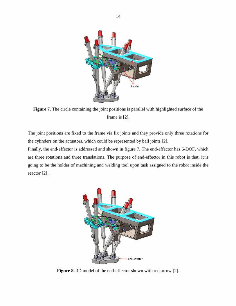
Figure 7. The circle containing the joint positions is parallel with highlighted surface of the
frame is [2].
The joint positions are fixed to the frame via fix joints and they provide only three rotations for
the cylinders on the actuators, which could be represented by ball joints [2].
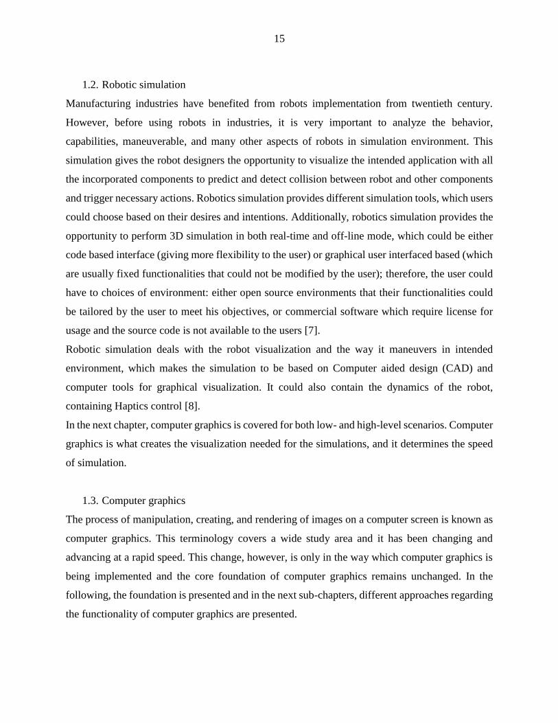
Finally, the end-effector is addressed and shown in figure 7. The end-effector has 6-DOF, which
are three rotations and three translations. The purpose of end-effector in this robot is that, it is
going to be the holder of machining and welding tool upon task assigned to the robot inside the
reactor [2] .
Figure 8. 3D model of the end-effector shown with red arrow [2].
15
1.2. Robotic simulation
Manufacturing industries have benefited from robots implementation from twentieth century.
However, before using robots in industries, it is very important to analyze the behavior,
capabilities, maneuverable, and many other aspects of robots in simulation environment. This
simulation gives the robot designers the opportunity to visualize the intended application with all
the incorporated components to predict and detect collision between robot and other components
and trigger necessary actions. Robotics simulation provides different simulation tools, which users
could choose based on their desires and intentions. Additionally, robotics simulation provides the
opportunity to perform 3D simulation in both real-time and off-line mode, which could be either
code based interface (giving more flexibility to the user) or graphical user interfaced based (which
are usually fixed functionalities that could not be modified by the user); therefore, the user could
have to choices of environment: either open source environments that their functionalities could
be tailored by the user to meet his objectives, or commercial software which require license for
usage and the source code is not available to the users [7].
Robotic simulation deals with the robot visualization and the way it maneuvers in intended
environment, which makes the simulation to be based on Computer aided design (CAD) and
computer tools for graphical visualization. It could also contain the dynamics of the robot,
containing Haptics control [8].
In the next chapter, computer graphics is covered for both low- and high-level scenarios. Computer
graphics is what creates the visualization needed for the simulations, and it determines the speed
of simulation.
1.3. Computer graphics
The process of manipulation, creating, and rendering of images on a computer screen is known as
computer graphics. This terminology covers a wide study area and it has been changing and
advancing at a rapid speed. This change, however, is only in the way which computer graphics is
being implemented and the core foundation of computer graphics remains unchanged. In the
following, the foundation is presented and in the next sub-chapters, different approaches regarding
the functionality of computer graphics are presented.
16
Pixels, when combined together, create images on the computer screens. Even the screen is
composed of pixels being put together in a rectangular shaped grid. These grids consist of rows
and columns and their pixels are so small that could not be captured with human eye. When the
resolution increases, these pixels become literally invisible. Pixels also have color characteristics;
each pixel can only show one color at a time. New screens are mostly using 24-bit color
configuration, in which colors are specified by three 8-bit numbers, ranging from zero to one
representing the amount of red, green, and blue (RGB). Any combination of these primary colors
could create a certain custom color.
The values of the colors for each pixel is stored stack of memories known as a frame buffer.
Therefore, if one attempted to change the color of any of the pixels, changes must be made inside
the stored values in frame buffer. It was mentioned that the screen is made of combination of pixels
and each pixels could have a custom color. To draw the screen, what we see on the monitor, screen
is redrawn at a fast rate up to 60 frames per second. The faster the screen is redrawn, smoother it
becomes to notice any change of color while manipulating color values in frame buffer. The
process of redrawing the screen per second is referred to as rasterization.
The above-mentioned method was the old approach of image rendering in computer graphics and
it is no longer an optimum way for pixel manipulation. Instead, the new approach of vector
graphics emerged which functioned on top of color manipulation of pixels via frame buffers.
Vector graphics introduced concept of specifying geometric objects (primitives) that have certain
attributes of line width and fling color. These primitives are circles, lines (straight or curved),
triangles, and rectangles [9]. At this point, two different categories of computer graphics
implementation emerges, which are low-level APIs and simulation software. Depending on the
objective of project and required functionalities, it is the user’s choice to decide which approach
meets their requirements. The difference between these two categories are covered when
comparing each environment and their characteristics will be discussed as well.
1.4. Simulation environment options
1.4.1. OpenGL
Silicon Graphics released the original version of OpenGL in 1992 Silicon Graphics had long
history in providing graphical workstations, which were usually powerful, expensive computers
for variety of industrial graphical applications. Most computers graphics hardware these days,
17
support OpenGL, including even mobile devices. Initially in desktop computers, CPU (Central
Processing Unit) handled the graphical contents of the screen. Drawing and rendering a line
segment on the screen, as an example, required the CPU to set the color of each pixel on the line
segment by running series of loops. The CPU performance dropped significantly when trying to
render multiple geometries; because, the more the number of pixels, the longer it took the CPU to
loop through each pixels color attribute to retrieve and change their values, which resulted in a
poor graphics performance.
Graphics processing these days is done by a specialized component called a Graphics processing
Unit (GPU). In this component, there multiple processors that working together in parallel that
increase graphical operations. Additionally, it has certain local memories coordinates and custom
images. The benefit of using GPU is that the processors in GPU have much faster access to the
data stored in GPU that accessing data stored in CPU. As a result, most of the graphical processes
are diverted from CPU and GPU is taking charge instead; the same example of line segment
drawing in new graphical systems, would be CPU sending necessary data and commands to GPU
without having to process any graphical data. These sets of commands that is understandable for
GPU are called GPU specific API (Application Programming Interface). OpenGL is one graphics
API example. As mentioned before, OpenGL is still compatible with new systems and they can be
translated to any language that GPU understands in case other graphical processing units are used.
The idea behind designing OpenGL was incorporating client/server abstractions. The unit which
controls the rendering and graphical computations is the server, which in this case is the GPU. The
server receives commands from the client; the commands are received from client and sent to
processing units and memories of server (GPU). The client is CPU and it is on the same computer
along with any other application program included on the hardware.
Three are two ways to pass OpenGL commands from CPU over to the GPU; it could be either
from the program, which is running on the CPU, or sending commands remotely over a custom
network. In the remote connection case, the client (OpenGL) is on one computer and the server
(CPU) on another computer. In this way, the graphical computations are done on the computer
using OpenGL as the client. This capability confirms the face that the server and client abstractions
are separate components and these two components are connected together via a channel, which
is responsible for sending the OpenGL commands. The drawback of this concept is that this
channel has a certain capacity and transferring commands take time through the channel; for
18
instance, if the line segment rendering takes microseconds from GPU, but communication time
via the channel takes milliseconds to happen. Therefore, fast graphical processing of GPU would
not be noticed as communication time is slowing down the process.
Therefore, developers started working on the minimization of communication time between CPU
and GPU. One idea was to collect all the data GPU needs for graphical processing and then
collecting all the data and sending it to the GPU; sending and storing required data in the GPU
memory only once, not only decreases the communication time, but it also makes it easier for the
GPU to access the data from its own memory whenever it is needed. Another idea was to minimize
the number of commands sent from CPU to the GPU for rendering processes; taking the line
segment drawing again as example, OpenGL requires one function for pixel rendering, one
function for pixels color attribute, and another function for pixels coordinates. This way, only for
a simple line segment, OpenGL requires three functions (commands) to perform the required task,
and if any of the attributes in pixels configurations needs to be modified, further commands are
needed.as the graphical rendering process is not limited to line segments and there are more
complicated geometries involved in every design, this way of working was not efficient at all in
earlier versions of OpenGL. Newer versions of OpenGL implemented commands with which all
the required data for the GPU could be sent by only passing arrays of information, which aided to
send all the commands as one command. However, if more instances of one object was needed in
a project, which command had to be called repeatedly. Later on, a new concept emerged that
reduced the number of command transmission; vertex buffer object (VBO) was a memory block
inside of the GPU allowing the GPU to store the attributes of pixels, therefore, these attribute did
not have to be sent to GPU from CPU as GPU could easily retrieve the required values. This
method was particularly useful for drawing primitives, and along with the GPU capability of
saving images as textures, revolutionized the computer graphics industry [9].
1.4.2. Direct3D
Another low-level rendering library for graphical representation is Direct3D. Just like OpenGL,
all graphics hardware available nowadays, support Direct3D, as its application-programing
interface (API) resembles the graphics pipeline infrastructure on the graphics card. The industries
using Direct3D are numerous and their application ranges from 3D CAD software, to medical
19
applications and game engines; the reason for such a wide variety of Direct3D implementation is
again efficient API in terms of speed and it’s compatibly with modern graphics hardware. Direct3D
is also taking advantage of the graphical processing unit (GPU); as GPU has its own processors
and the graphical calculations are happening in parallel with the processors, the CPU does not have
to compensate its memory to carry our graphical calculations. The way Dircet3D is communicates
with GPU is through shader API with C++, and .NET wrappers. Direct3D is also open-source
library available to the public and the functionalities included are the same as OpenGL; math
functions, image handling functions, texture generation, shader and mesh generation functions
[10].
As mentioned earlier, Direct3D is written with C++ and some .NET wrappers. However, that does
not mean that the users are doomed to use Direct3D only with C++ and there should be something,
which makes this API usable for other users with different programming language backgrounds.
Component Object Model (COM) is what makes Direct3D language independent and allows users
to use required functionalities via the provided API with other languages as well. COM is
implemented as an interface, which could be treated just like a C++ class. Most of the programmers
are familiar with pointers in object-oriented programming. The way a user acquire access to
Direct3D via other languages, is by getting a pointer to the COM. A user does not necessarily have
to know what these pointers do and how they do it, therefore, the majority of the process is
happening behind the scenes. It is important to note that after creating pointers to COM and
accessing their methods for various functionalities, must be terminated as well, they must be closed
as well and that is called releasing [10].
Direct3D also provide users with functionalities to handle textures in 2D. Textures in Direct3D
are matrices that have data elements, and as mentioned in the section for OpenGL, the data
elements represent certain attributes such as color and coordinates of the pixels. For now, we
assume that these data elements are only pixel attributes with vectors for position and colors, but
these data elements have a wider interpretation with respect to GPU [10].
In many 3D graphics application that involves animating sequence of pictures, there will be
noticeable changes in the brightness between the cycles displayed on the screen and this incidence
is called flickering. Low-level graphics like Direct3D and OpenGL implement a certain approach
with which flickering does not happen. They have two buffers, called the front and back buffer; to
prevent flickering, Direct3D renders the whole frame related to the moving pictures into the back
20
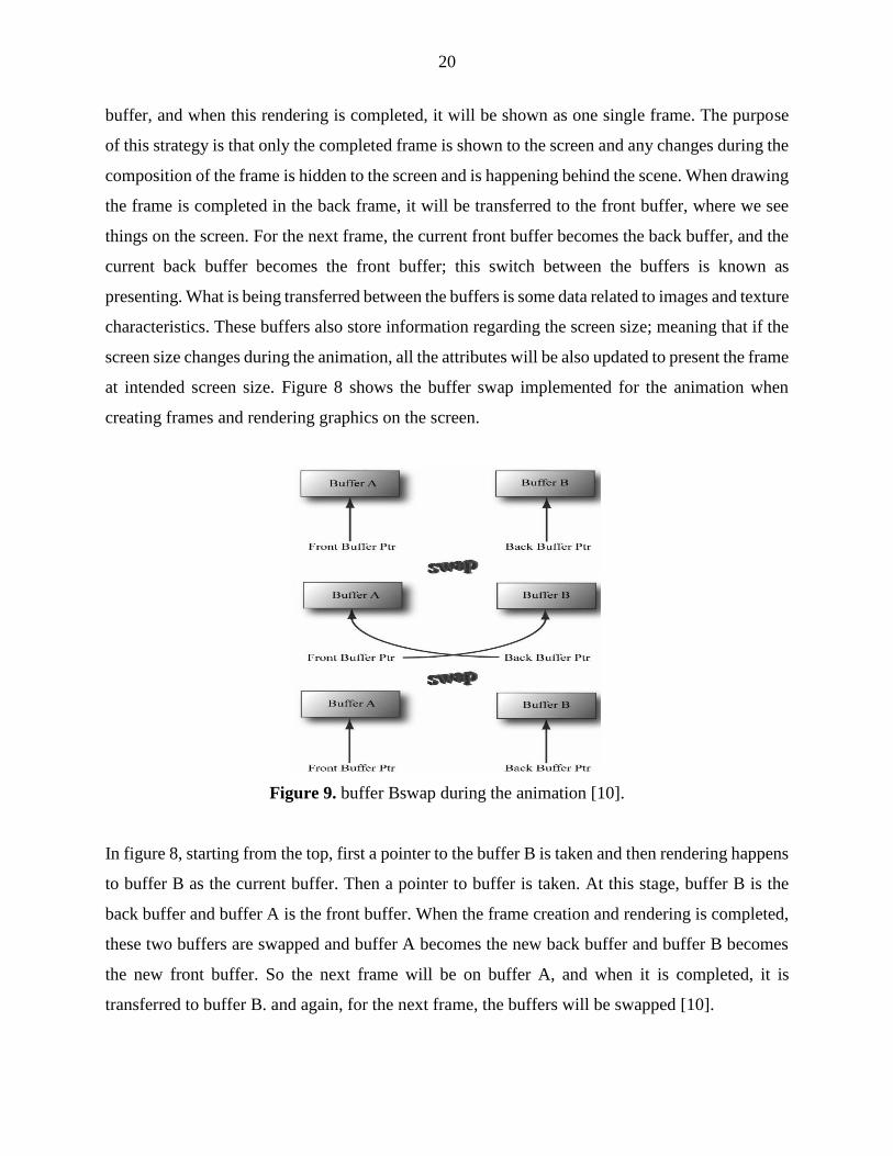
buffer, and when this rendering is completed, it will be shown as one single frame. The purpose
of this strategy is that only the completed frame is shown to the screen and any changes during the
composition of the frame is hidden to the screen and is happening behind the scene. When drawing
the frame is completed in the back frame, it will be transferred to the front buffer, where we see
things on the screen. For the next frame, the current front buffer becomes the back buffer, and the
current back buffer becomes the front buffer; this switch between the buffers is known as
presenting. What is being transferred between the buffers is some data related to images and texture
characteristics. These buffers also store information regarding the screen size; meaning that if the
screen size changes during the animation, all the attributes will be also updated to present the frame
at intended screen size. Figure 8 shows the buffer swap implemented for the animation when
creating frames and rendering graphics on the screen.
Figure 9. buffer Bswap during the animation [10].
In figure 8, starting from the top, first a pointer to the buffer B is taken and then rendering happens
to buffer B as the current buffer. Then a pointer to buffer is taken. At this stage, buffer B is the
back buffer and buffer A is the front buffer. When the frame creation and rendering is completed,
these two buffers are swapped and buffer A becomes the new back buffer and buffer B becomes
the new front buffer. So the next frame will be on buffer A, and when it is completed, it is
transferred to buffer B. and again, for the next frame, the buffers will be swapped [10].
21
1.4.3. VTK
Visualization Tool Kit (VTK) is an open source tool, working on top of OpenGL graphics API,
for scientific data processing, 3D visualization and simulation, and data analysis. The application
areas of VTK includes image processing in medical fields, molecule level visualization in
chemistry, fluid mechanics/dynamics, and finite element-based studies. The source code of VTK
is originally compiled with C++, however, one is not limited to C++ coding since there is the
possibility to use the VTK capabilities or even develop different modules with Python, Java, or
Tcl. The libraries of certain sets of functionalities and in terms of visualizations, all the primary
primitives are available for any geometry rendering process. The difference between VTK and
OpenGL/Dircet3D is that VTK is using the core graphical functionalities as a set of certain
functions; in OpenGL/Direct3D one has to hard code every graphical aspect from creating window
and putting pixels on screens, to finally drawing primitives for more complication geometries,
whereas in VTK, the graphical environment is already set up for window creation, camera and
light setup, and more importantly, there is no need to create geometries starting from pixels as
there functions such as Cylinder(), Sphere(), Cone(), and many other useful commands that aids
the programmers to focus more on other aspects. And as the source code is available, one could
easily access the libraries and change any of the functionalities for potential optimization or
development [11].
This toolkit was provided with the idea of object-oriented programming, allowing the users to
conveniently integrate available functionalities to different graphical projects [12]. The advantage
in using VTK over lower level graphics APIs is the fact users do not need to have sophisticated
knowledge of computer programming; because the purpose of VTK development was to provide
a toolset for the scientists and engineers to visualize and analyze their data, that would be a burden
if they had to deal with core graphical functionalities and graphics pipelines as they might not have
enough knowledge to start from using low level graphical functionalities [13]. The way OpenGL
is used in this toolset is that OpenGL is placed on the end of the pipeline of data, through which
the data is transmitted from OpenGL to the screen for rendering process. To check the quality of
this pipeline and to ensure that the data is being properly sent from OpenGL to VTK, there is a
functionality implemented on VTK (working in parallel) which automatically gets the pixel
attributes and check if there is any mismatch between the attributes sent from OpenGL to the VTK.
22
This monitoring layer has been a pivot point for VTK development as it verifies the functionality
of VTK in the interpretation of scientific data across different platform [11].
As mentioned earlier, VTK is wrapped in C++ and this source code must be obtained from the
VTK website and then built on any desired platform with CMake [14], which signifies the fact that
VTK could be a cross platform toolset that could be used multiple times [15].
1.4.4. Unity3D
The use of game engines has gained popularity in recent years and Unity3D is a platform
independent game engine, which gives the game developers to connect different platforms in small
teams. Unity3D is in fact a package of many other modules such as Android-based platforms,
Asset servers, and Pro version [16]. The convenient application of game engines including
Unity3D is the availability of Graphical user interface (GUI) which gives the user the ability to
create and visualize a scene without much computer programming knowledge. Games such as
Plants vs. Zombies, and The Fallen King are famous iPhone-based games developed in Unity3D.
Unity3D being as a game engine, does not mean that there is no way of coding and communicating
with the engine through APIs; the relationship between the objects in the game engine are handled
by C# and Java scripting languages. There are other communication possibilities involved;
however, these two programming languages access core functionalities. Should one user attempt
to hard code some modules of the game, the script must wrapped and compiled in a .dll file of type
.Net. The reason why Unity3D uses compiled .dll files is the performance speed of these libraries
compared to the running speed of raw Java codes for instance. The idea behind using high-level
programming languages in the game development with Unity3D is the fact that these languages
are platform independent, giving the developers the opportunity to develop their environments on
Windows, for instance, and running the game on a website using a plugin [17].
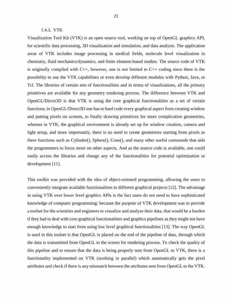
The programming architecture in Unity3D is based on numerous components that each have
different functionality in the game module. These functionalities could be implemented easily
multiple times in the game module. Game module consist of different game objects; these objects
contain various characteristics and attributes and depending on the game requirements, they could
be added to the game module. As an example, Box Collider is an object handling the collision
detection and scripts provide the game logic to the game module. The schematic of the Unity3D
game architecture is depicted in figure 8.
23
Figure 10. Unity3D game architecture using components [17].
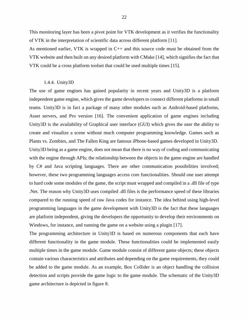
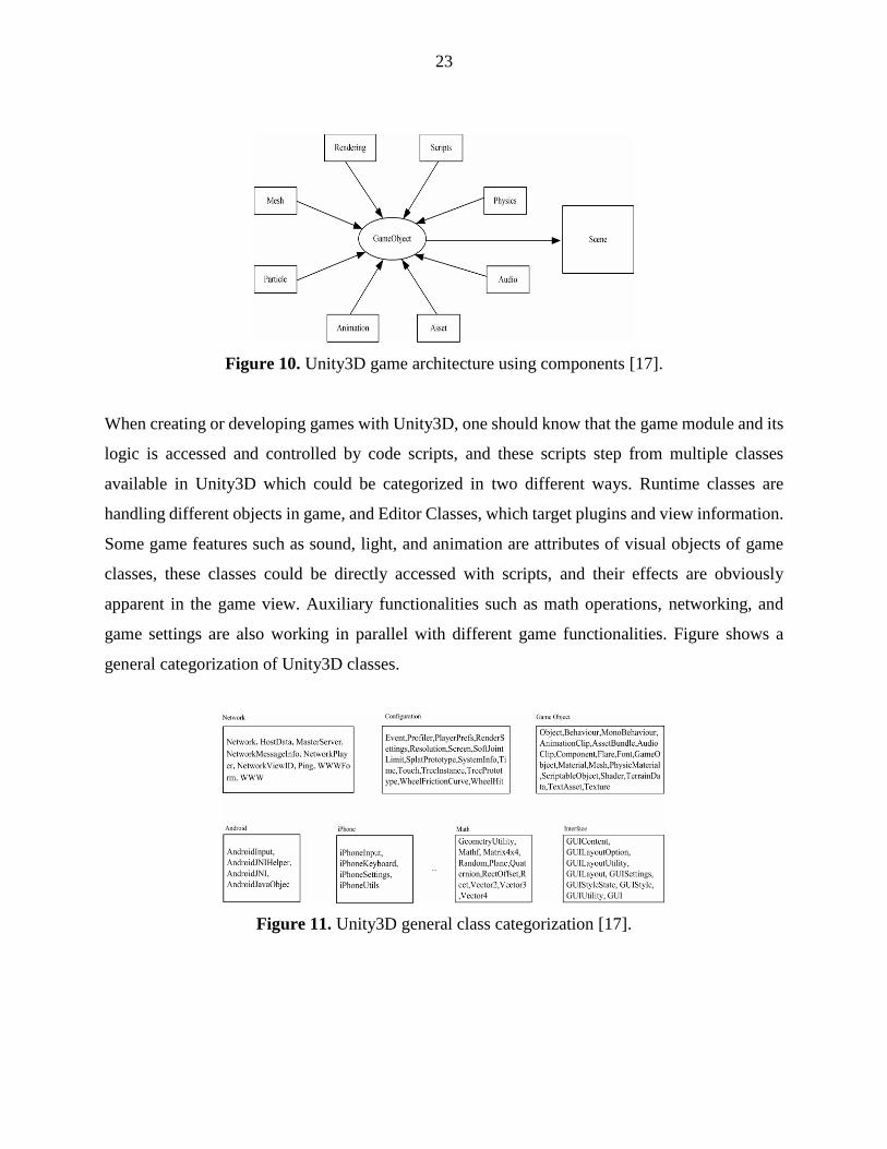
When creating or developing games with Unity3D, one should know that the game module and its
logic is accessed and controlled by code scripts, and these scripts step from multiple classes
available in Unity3D which could be categorized in two different ways. Runtime classes are
handling different objects in game, and Editor Classes, which target plugins and view information.
Some game features such as sound, light, and animation are attributes of visual objects of game
classes, these classes could be directly accessed with scripts, and their effects are obviously
apparent in the game view. Auxiliary functionalities such as math operations, networking, and
game settings are also working in parallel with different game functionalities. Figure shows a
general categorization of Unity3D classes.
Figure 11. Unity3D general class categorization [17].
24
1.4.5. SimMechanics
SimMechanics is an environment based on implementing Simulink block diagrams in order to
model the mechanical systems that implement standard laws of Newton. The kinematical analyses
in SimMechanics environment do not require deriving the kinematic equations of a system; block
diagrams are representatives of mechanical components, which speeds up the modeling process.
This is particularly helpful when the derivation of equations of motion for a mechanical system
becomes complicated. SimMechanics is implemented on MATLAB from version 6.5, it is a toolset
for the Simulink simulation environment with graphical user interface, and it utilizes six series of
libraries for discrete functionalities. The SimMechanics functionalities are accessible from
Simulink blocks and each block is a representative of a certain part of studied mechanical system;
there are blocks for body geometries, implemented sensors, and the joint between the bodies that
connect them define degree of freedom. To demonstrate how SimMechanics is used in study of
multibody simulations, an example of a mechanical system is presented and then the system model
is prepared in SimMechanics with Simulink blocks and presented with figures [18].
The example taken from a study was an inverted pendulum, which is in the categorization of
systems with multiple variables, non-linear systems of high order, and unstable systems. Deriving
mathematical model of the system is challenging. Additionally, if a control algorithm is meant to
be provided for such a system, is going to be inefficient compared to a linear system and it requires
approximations, which are usually inaccurate. SimMechanics provides a better alternative as it
does not derive the mathematical model of mechanical systems in a direct way [18]. It is important
to mention, that illustrating this example is only for the purpose of gaining familiarity with
SimMechanics and Simulink environment and solving equations of motion and studying the
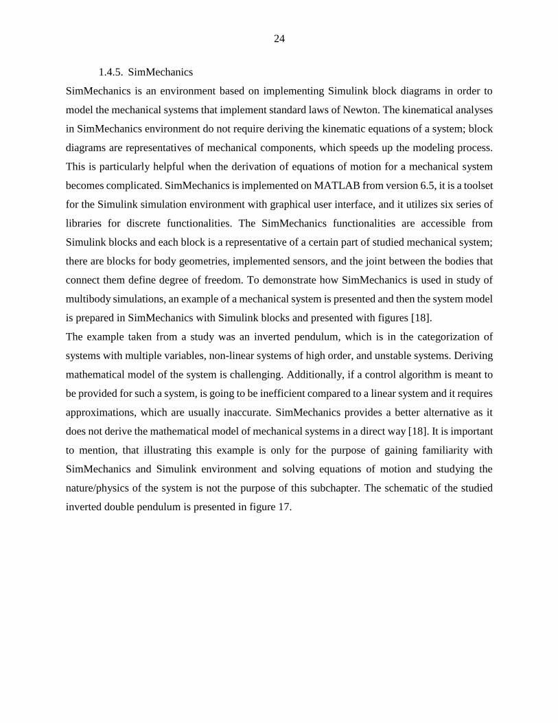
nature/physics of the system is not the purpose of this subchapter. The schematic of the studied
inverted double pendulum is presented in figure 17.
25
Figure 12. schematic of inverted double pendulum [18].
The double pendulum shown above has four major parts as its skeleton; a rail, which is shown
with two parallel lines, the black box representing a cart, and two rods. In this study, the bodies
were considered rigid. Cart is attached to the rail via a prismatic/translational joint and it only has
one degrees of freedom, meaning that it can only slide alongside the rail (the cart is moved by a
driving unit, which is not shown in this picture). Rod 1 is attached to the cart via a revolute joint
and it can only rotate in the same plane as cart (a revolute joint leaves only one degree of freedom
as a rotation). Rod number two is also attached to rod number one with revolute joint, which
provides also one degree of freedom as rotation in the same plane as cart and rod one.
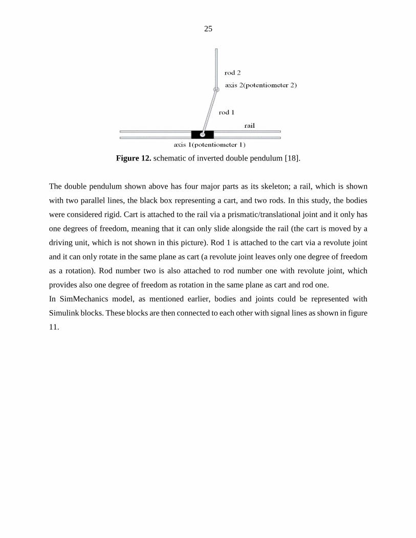
In SimMechanics model, as mentioned earlier, bodies and joints could be represented with
Simulink blocks. These blocks are then connected to each other with signal lines as shown in figure
11.
26
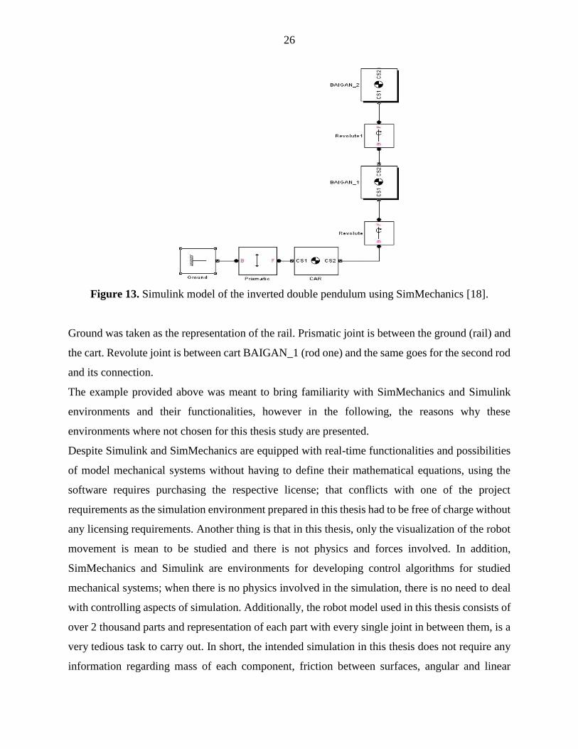
Figure 13. Simulink model of the inverted double pendulum using SimMechanics [18].
Ground was taken as the representation of the rail. Prismatic joint is between the ground (rail) and
the cart. Revolute joint is between cart BAIGAN_1 (rod one) and the same goes for the second rod
and its connection.
The example provided above was meant to bring familiarity with SimMechanics and Simulink
environments and their functionalities, however in the following, the reasons why these
environments where not chosen for this thesis study are presented.
Despite Simulink and SimMechanics are equipped with real-time functionalities and possibilities
of model mechanical systems without having to define their mathematical equations, using the
software requires purchasing the respective license; that conflicts with one of the project
requirements as the simulation environment prepared in this thesis had to be free of charge without
any licensing requirements. Another thing is that in this thesis, only the visualization of the robot
movement is mean to be studied and there is not physics and forces involved. In addition,
SimMechanics and Simulink are environments for developing control algorithms for studied
mechanical systems; when there is no physics involved in the simulation, there is no need to deal
with controlling aspects of simulation. Additionally, the robot model used in this thesis consists of
over 2 thousand parts and representation of each part with every single joint in between them, is a
very tedious task to carry out. In short, the intended simulation in this thesis does not require any
information regarding mass of each component, friction between surfaces, angular and linear
27
speeds, damping and stiffness coefficients, and many other parameters that are inputs for
simulation of mechanical systems using SimMechanics in Simulink.
1.4.6. ROS
ROS (Robot Operating System) is an open-source toolset for robotic operations. Referring to ROS
terminology, it comprises structured layer of communication on top of the operating systems.
Initially, ROS design intention was to handle the difficulties in the process of service robots
development in large applications [19].
ROS architecture consists of three elements: nodes, topics, and services. In the following, a general
description of each of these nodes are presented, and at the end, some of the reasons why this tool
was not used in this thesis are mentioned [20].
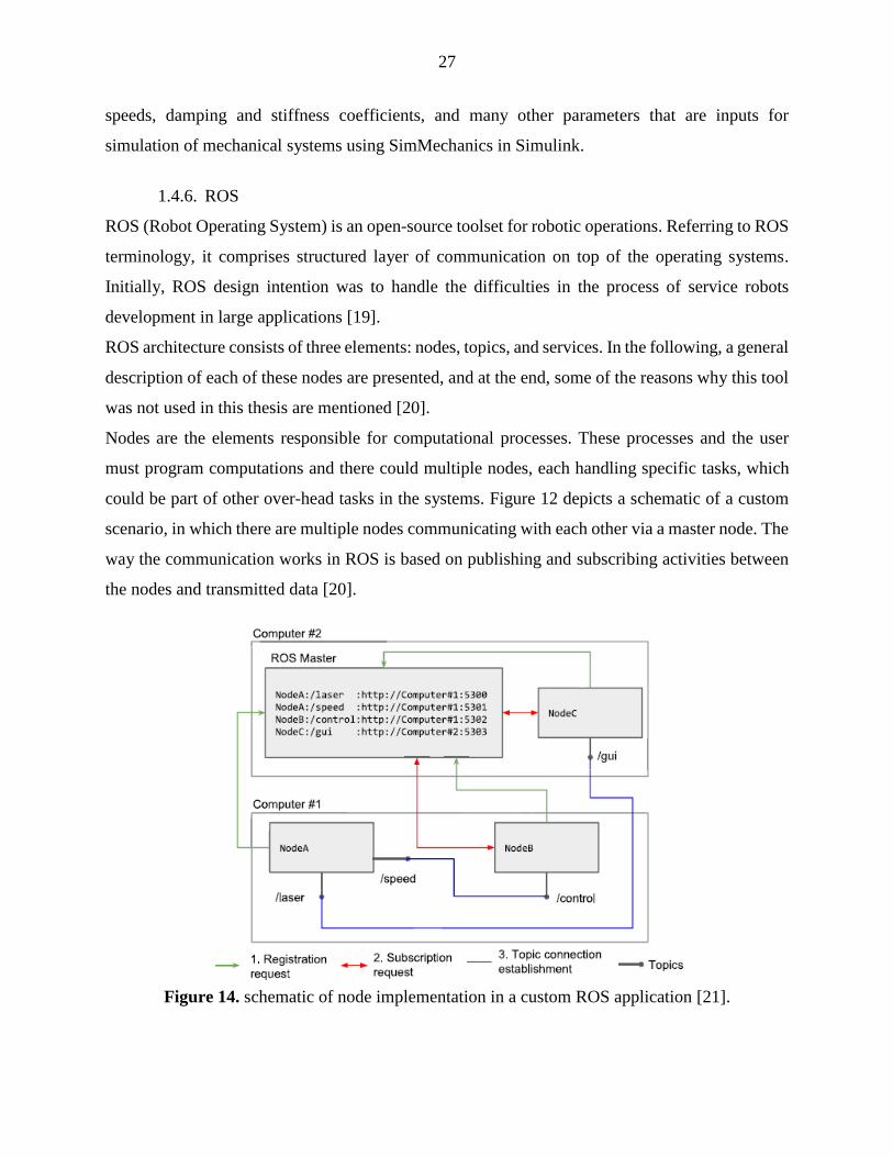
Nodes are the elements responsible for computational processes. These processes and the user
must program computations and there could multiple nodes, each handling specific tasks, which
could be part of other over-head tasks in the systems. Figure 12 depicts a schematic of a custom
scenario, in which there are multiple nodes communicating with each other via a master node. The
way the communication works in ROS is based on publishing and subscribing activities between
the nodes and transmitted data [20].
Figure 14. schematic of node implementation in a custom ROS application [21].
28
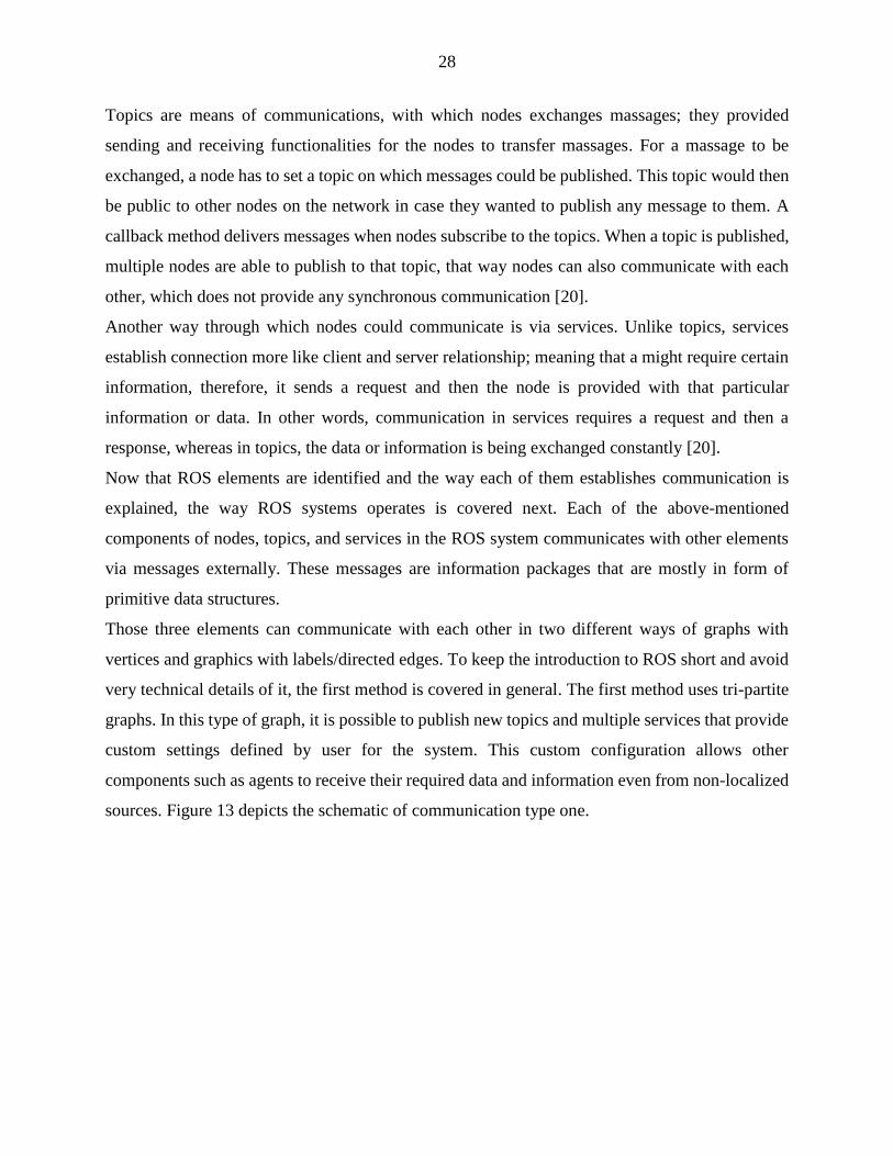
Topics are means of communications, with which nodes exchanges massages; they provided
sending and receiving functionalities for the nodes to transfer massages. For a massage to be
exchanged, a node has to set a topic on which messages could be published. This topic would then
be public to other nodes on the network in case they wanted to publish any message to them. A
callback method delivers messages when nodes subscribe to the topics. When a topic is published,
multiple nodes are able to publish to that topic, that way nodes can also communicate with each
other, which does not provide any synchronous communication [20].
Another way through which nodes could communicate is via services. Unlike topics, services
establish connection more like client and server relationship; meaning that a might require certain
information, therefore, it sends a request and then the node is provided with that particular
information or data. In other words, communication in services requires a request and then a
response, whereas in topics, the data or information is being exchanged constantly [20].
Now that ROS elements are identified and the way each of them establishes communication is
explained, the way ROS systems operates is covered next. Each of the above-mentioned
components of nodes, topics, and services in the ROS system communicates with other elements
via messages externally. These messages are information packages that are mostly in form of
primitive data structures.
Those three elements can communicate with each other in two different ways of graphs with
vertices and graphics with labels/directed edges. To keep the introduction to ROS short and avoid
very technical details of it, the first method is covered in general. The first method uses tri-partite
graphs. In this type of graph, it is possible to publish new topics and multiple services that provide
custom settings defined by user for the system. This custom configuration allows other
components such as agents to receive their required data and information even from non-localized
sources. Figure 13 depicts the schematic of communication type one.
29
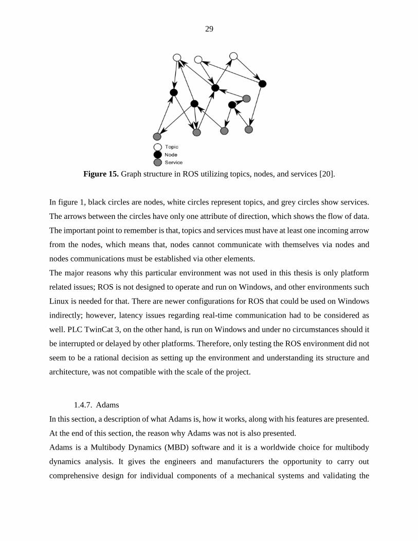
Figure 15. Graph structure in ROS utilizing topics, nodes, and services [20].
In figure 1, black circles are nodes, white circles represent topics, and grey circles show services.
The arrows between the circles have only one attribute of direction, which shows the flow of data.
The important point to remember is that, topics and services must have at least one incoming arrow
from the nodes, which means that, nodes cannot communicate with themselves via nodes and
nodes communications must be established via other elements.
The major reasons why this particular environment was not used in this thesis is only platform
related issues; ROS is not designed to operate and run on Windows, and other environments such
Linux is needed for that. There are newer configurations for ROS that could be used on Windows
indirectly; however, latency issues regarding real-time communication had to be considered as
well. PLC TwinCat 3, on the other hand, is run on Windows and under no circumstances should it
be interrupted or delayed by other platforms. Therefore, only testing the ROS environment did not
seem to be a rational decision as setting up the environment and understanding its structure and
architecture, was not compatible with the scale of the project.
1.4.7. Adams
In this section, a description of what Adams is, how it works, along with his features are presented.
At the end of this section, the reason why Adams was not is also presented.
Adams is a Multibody Dynamics (MBD) software and it is a worldwide choice for multibody
dynamics analysis. It gives the engineers and manufacturers the opportunity to carry out
comprehensive design for individual components of a mechanical systems and validating the
30
model dynamics behavior prior to any real-time implementation. Discrete system characteristics
such as motion analysis, structural analysis, joints behavior, and even applied control scenarios
could be evaluated by means of features provided by Adams. This is particularly beneficial for
systems with non-linear dynamic equations that could be solved quickly as their interpretations
are being used by finite element analysis [22].
Some of the application areas of Adams in multibody dynamics are found from literature reviews
and they are presented as following: ride comfort of a vehicle was studied by evaluating one-fourth
of the structure considering multiple variables. The model that was implemented in Adams had
shown very close behavior with respect to the actual test scenario, therefore, this validation was
approved for further development of the model and also confirmed Adams competence for this purpose
[23].
In another study, a Stirling engine was simulated in the Adams and then the functionality of the engine
was optimized; using Adams software, it was possible to carry out this simulation considering gas
forces, friction forces and temperature related behaviors of the different motor components and
auxiliary parts [24].
Or, modeling and development of pistons of air compressors was carried out to analyze mechanical
properties of mechanical systems that have specific constraints; in that study, the mechanical system
was considered with both rigid and deformable components and non-linear system equations were
solved with Adams solver and it provided promising results for the virtual prototyping [25].
The first reason why Adams software was not used is the license purchase requirement for using the
product, which conflicts with thesis requirements. Secondly, Adams software is not an open-source
platform, meaning that source code of the software is not available to the public, making it a
commercial package for the users [22].
1.4.8. Unreal Engine
Unreal Engine was first created in late 1990s and the idea behind its evolution was to have a feeling
of first-person shooter. Unreal Engine is a game engine, which has a combination crucial
functionality for any game application such as default/custom collision detection, artificial
intelligence (AI), connectivity to other networks, scripting interface, and many other built in
features. The popularity of Unreal Engine (UE) is because of one very important characteristic,
which is the game architecture; the game architecture consists of modules, which could be accessed
31
and implemented in every stage of the game working in parallel with other modules. The very
unique characteristic that makes these modules and the while game engine in general so popular,
is the UE scripting language; this scripting language is C++ based to the most part and it gives the
users full control over the maneuverability over the game modules. UE is a game engine, which
does not require users to buy license for its use and small-scaled developments. The source code
is also available on the GitHub and it could be easily accessed for development purposes. UE not
only is supported on Windows systems with compatible graphics hardware configurations, but it
is also supported to be used on Xbox. UE is working on top of the low-level libraries such as
OpenGL and Direct3D; therefore, it gives users the freedom to further develop custom
functionalities to other environments such as Android and IOS. The biggest advantage of UE over
other game engines such as Unity, is their very recent visual scripting language called Blueprints
(BP); BPs provide users with the majority of the UE functionalities and it is specifically beneficial
for the game engine users that do not have very sophisticated programming knowledge of C++ in
particular [26].
There is also a certain community for UE users and they target all the UE aspects concerning very
basic introduction for very new users, and development news for advanced users who are
constantly implementing or developing UE functionalities. It also keeps users and developers
updated with latest modifications and market insights, which is a unique environment compared
to other game engines.
There are several component in UE game engine which are organized in way that they work in
parallel without affecting other components if the experienced any change or major modification.
These components could also be called engines and in the following, these engines are described
very briefly to make users familiar to the engine environment. The first engine is the graphics
engine; the graphics engine is responsible for the graphical calculations, frame creation, rendering
process, lighting, and shading. It is important to note that the graphics engine is not limited to
above-mentioned tasks and there are more objectives involved. The graphics engine decides, for
instance, which objects should appear first on the screen, or which objects should appear behind
or in front of other objects. As mentioned earlier, graphical calculations also include textures,
shaders, and materials. The aspects and attributes are assigned to the objects being rendered on the
screen [27].
32
Another engine or component in UE is the sound engine; as the name implies, the sound engine
provides the sound effects for the game. These sounds are assigned to the objects present in the
game, but they are organized as sequence of events; for instance if and object falls down, the sound
assigned to this particular event and for this particular object is streamed. Or explosion and engine
start also have their own sound effect attributes that will be emitted when their sequence comes
into game play [27].
The next engine is the physics engine and to illustrate their importance and functionality, we go to
different simulation approaches; there are two ways with which a simulation could be performed:
either kinematic simulation, or dynamic simulation. In kinematics simulation, the movement of
the objects or mechanisms are studied without considering the existing forces. Whereas in dynamic
simulations, the existing forces are also considered in the simulation. Physics engine works just
like dynamic simulations, meaning that every object in the game play could have mass and
therefore, other external forces such as gravity, friction, and damping are included. Implementing
physics engine in simulations make them look more believable and realistic; if a ball hits the
ground, users can see it bouncing. Alternatively, if a flag is being used in the game, the flag’s
texture and mesh could be updated in each frame with wind blow dynamically, making it more
realistic. In addition, the mechanisms such as robots could be imported into the UE environment
and they could be simulated based on physics by providing the mass, stiffness, friction, and proper
damping values. The advantage of using this method is that when simulating robots with numerous
joints and actuators, it would be a very tedious job to define the motions in each one of the joints
mathematically, and instead, users could easily place physical joints such as revolute joints and
limit the motion with this particular approach [27].
As game engines are for game development purposes, they require interaction between the user
and the players inside the game; if the game scenario is a first-person shooter, in order to be able
to use the for shooting, or picking up objects or any other interaction, the user should be able to do
that with mouse clicks and key-pressing on the keyboard. This interaction is managed by the input
manager [27].
UE also provides game play across a network rather than a solo player in the game mode; this
gives the players the opportunity to compete in different games across a network handle by the UE
network infrastructure; this network infrastructure provides a server to which multiple players
could be connected and they can interact with other players in real-time [27].
33
1.5. PLC
The advances in automation industries has increased the number robots with various tasks at
different stages. In order to make sure that tasks will be accomplished properly and safely, control
algorithms implemented by engineers have to be robust and stable.to ensure the robustness and
reliability of the control algorithm, there should be the possibility of programming the control
algorithms. PLC stands for Programmable Logical Controller is a processor unit that works on
Windows and is responsible for controlling robots or mechanisms used in automation industries
[28].
Logic refers to the brain or the control algorithm, which is triggered by switches; for instance, if a
motor or a system is to be turned on, off, or in any other condition, a switch will activate and
trigger the PLC. Therefore, the switch becomes the input to the PLC and PLC is connected to the
output system. There are two major parts that PLC is based on; the programming logic and the
PLC device. In the following, these two parts will be covered in detail to have a better
understanding of how PLC actually works [28].
PLCs, nowadays, are meant for controlling different processes and they operation-using
computers. The way they work is they get the necessary data from system sensors as inputs and
they update actuators and motor drives of the system based the system state at a given time. PLC
has its own processors, which is connected to chips of input/output, and memory in parallel via
control buses, some data, and specific addresses. Unlike computers, PLC does not have storages
like hard-drives; instead, they have solid-state memory to save in their programs. PLCs give the
users to monitor the process by its build in visualization, which works as an interface between
machines and humans known as Human Machine Interface (HMI). PLCs have sockets for
input/output devices that they could be communicating with each other via specific ports. PLCs
are designed to perform predefined tasks; these tasks, like the way compilers run codes, are
performed in order from start to finish and one by one. PLC devices are also designed to maintain
their functionalities in harsh environments; just like any other industrial application oriented
computer, PLC devices must be able to operate under various temperatures and different levels of
moisture content. Usually in factories and other industrial environments, there is possibility of
sudden voltage changes, or even existence of gases that could chemically react with different parts
of the devices [28].
34
The ease of installation and maintenance in PLC devices were key in their design. The HMI also
made the fault diagnosis very easy by prompting and showing error messages in the different parts
of the circuit. The PLC has its own build it language, which could be implemented in various forms
of function blocks, ladder diagrams, or even structured text [28].
1.5.1. PLC communication options
Now that the PLC architecture and mechanism has been explained, there should be ways to connect
PLC to the intended simulation environment in order to be able to use the modules and
functionalities of the PLC for the control of robot in the simulation.
According to the Beckhoff documentation, there are various different ways to connect one PLC
TwinCat module to other environments. Depending on the type of the secondary environment,
specific connections are available and each require certain configurations. These configurations
are applied partially to the first PLC module as well as on the operating system (Windows in this
thesis) on which PLC is running. It is important to note, that PLC could also be run on virtual
machines and it does not have to be necessarily on Windows, however, one should be aware of the
latency aspects required for the intended project. The choice of connection type is primarily based
on the type of the second environment being connected to the PLC; two scenarios are possible
with respect to this matter: wither the second environment is also a PLC module, or the second
environment is not a PLC module [29]. In this thesis, the second environment is not a PLC module.
As there are many communication types for PLC TwinCAT 3, they cannot be explained one by
one in detail here and only real-time communications of “TCP/UDP real-time” and ADS C++ are
explained as they are more relevant to the purpose of this thesis.
TCP and UDP are protocols for data or information transportation which are internet based
communication means. To establish and use these protocols, there must be a link between the
specific libraries needed to use these protocols and their functionalities.
TCP stands for Transmission Control Protocol and it is connection based belonging to telephone
connection group. In this type of communication, in order to be able to send and receive
information over the protocol, users on the either end of the protocol has to set the connection prior
to communication. The information being transmitted via this type of communication protocol is
a structure of bytes. The TCP connection protocol is based on the delivery messages; meaning that
35
if a server or a client sends a structure of data and information to another end of the TCP port, the
receiver must approve that the structure has been received, otherwise, the data stream will not
continue. The way these structures of data are sent over TCP protocol is, that the data should be in
a specific format that is readable for the receiver and that is the only thing the receiver requires
from the sender. Other than that, the receiver does not even know the origin of the data structure
or even where the data transmission is going to be stopped. As well as the type of data structure
sent by the sender to the receiver, the receiver should also know the size of the data that it is going
to receive. In general, TCP protocol has a server and a client and they each need specific
functionalities to be assigned to them in order to be properly stablished on the either side of the
network [29].
TCP client needs be able to open and close the communication port; it is important to note that, in
the server and client communications, server is stand-by and waiting for the client for any request
or command and that does not mean that the client is controlling the server. The server starts
responding whenever the client needs any specific information. Therefore, the client should be
able to handle the port when connecting to the server. Another functionality that the client needs
to have is being able to send and receive data to and from the server; this functionality must be
clarified for the client [29].
TCP server on the other hand, acts as a listener, meaning that it waits for the client for the requests
and commands. Previously it was mentioned that the client should be able to handle the connection
port, however, that does mean that server cannot have any control over the port of communication;
there are many cases in which the client and server are connected together and the client requests
for specific data or information from the server, however, for some reason the server finds the
client struggling to send or receive messages and required confirmation for message delivery. In
that case, the server should also be able to handle the communication port to at least save some
performance and to be available for other clients. The TCP server should also be equipped with
functionalities for data transmission. TCP server should also have access to PLC runtime module
to be able to handle that communication. The last feature or functionality of the server is
something, which is called polling. Polling is a function block implemented in the PLC runtime
module, which is being called periodically for data transmission [29].
Another protocol is the UDP protocol, which is the short form of User Datagram Protocol. Unlike
TCP, UDP does not require specific connection between the server and the client. Another
36
difference between the TCP connection and the UDP connection is in the way that data is
transmitted via the communication port. UDP transfers packages of data rather than structures of
data. Additionally, in UDP based communication, the server keeps sending the data to the client
without the need for any confirmation from the receiver or the client that the data packet has been
delivered. This way of communication places, a significant advantage on the UDP based
communication over the TCP based communication. And the reason being is, that in the TCP based
communication, the server waits for the client to send the delivery confirmation and it does not
send any more data until the confirmation is received; if wither of the server or the client fail to
received or send the confirmation, the communication is interrupted and slowed down. The same
features and requirements mentioned for the TCP communication are also needed for the UDP
connection means, therefore, there is no need to repeat the same content for this part as well [29].
The reason why any of the TCP or UDP cannot be implemented in this study is that, these two
communication means require either two separate machines (meaning two discrete IP addresses)
or a secondary Ethernet Cad card on the same computer with a loop cable. The latter is only for
testing purposes and cannot be used for real-time communication. In other words, TCP and UDP
are for local communication and as only one computer was available for this thesis, they could not
be used [29].
Another way of PLC communication with a secondary environment is via Automation Device
Specification or in short form known as ADS. The advantage of this type of communication is that
they are not internet based; instead, they use dynamic libraries that are compiled by the Beckhoff
Company. These dynamic libraries are based on the C++ modules of the PLC TwinCat and they
are available to the public. The way these libraries are implemented into the communication over
ADS is that server and client transmit data using pointers to the functions and methods inside of
the C++ modules for the PLC. In order to use these functionalities, one should include the
necessary libraries into the source project for the simulation and recompile the source project [29].
37
2. THESIS OBJECTIVE AND MOTIVATION
The purpose of this thesis is to prepare a real-time 3D simulation environment that could be
linked to PLC TwinCat 3 for controlling purposes. However, before diving into the technicality
of the setup in thesis and explaining how the environment is set up, it is crucial to understand
the actual scenario in which the robot is going to be implemented.
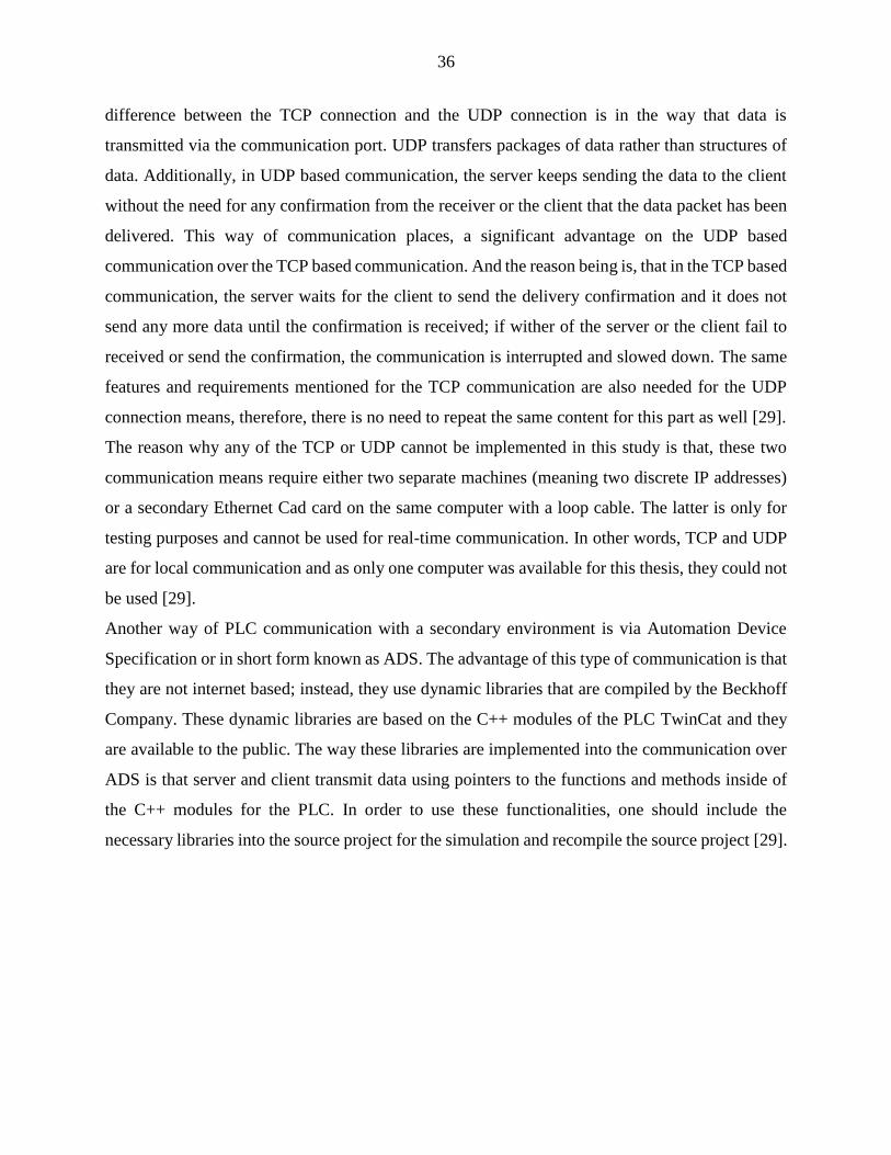
As mentioned earlier, the studied parallel robot is responsible for welding and machining of
the intersector inside of the vacuum vessel in the ITER fusion reactor. A schematic of the actual
space inside of the vacuum vessel of the ITER fusion reactor is presented in figure 16. Figure
16 shows the vacuum vessel subject to welding; the track rail is also in orange color. In the
same figure, the parallel manipulator is also shown in the bottom right-hand corner of the
picture.
Figure 16. ITER vacuum vessel schematic with the track rail and the parallel manipulator [1].
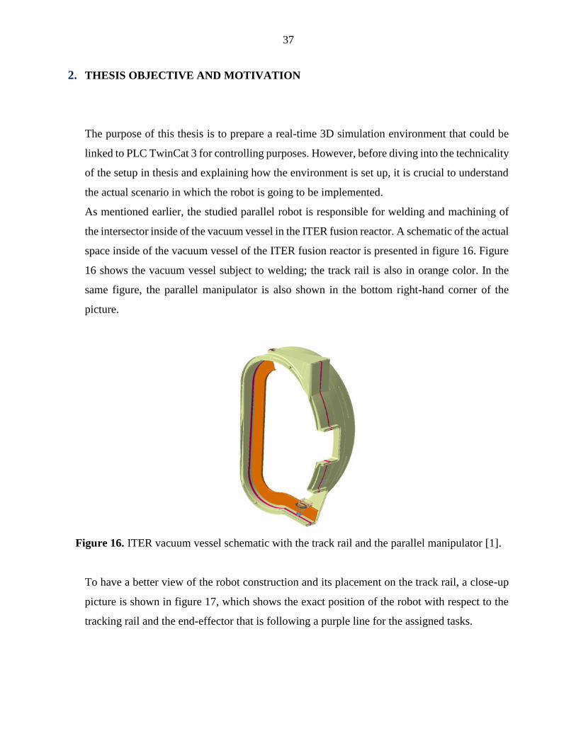
To have a better view of the robot construction and its placement on the track rail, a close-up
picture is shown in figure 17, which shows the exact position of the robot with respect to the
tracking rail and the end-effector that is following a purple line for the assigned tasks.
38
Figure 17. Close-up section of the ITER vacuum vessel with end-effector path and robot
placement with respect to the track rail [1].
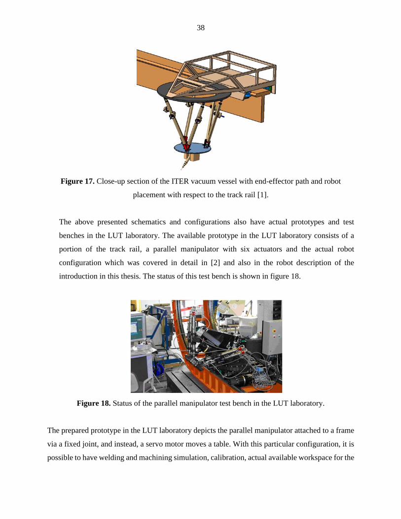
The above presented schematics and configurations also have actual prototypes and test
benches in the LUT laboratory. The available prototype in the LUT laboratory consists of a
portion of the track rail, a parallel manipulator with six actuators and the actual robot
configuration which was covered in detail in [2] and also in the robot description of the
introduction in this thesis. The status of this test bench is shown in figure 18.
Figure 18. Status of the parallel manipulator test bench in the LUT laboratory.
The prepared prototype in the LUT laboratory depicts the parallel manipulator attached to a frame
via a fixed joint, and instead, a servo motor moves a table. With this particular configuration, it is
possible to have welding and machining simulation, calibration, actual available workspace for the
39
manipulator, as well as decent accuracy in terms of position control. The available workspace for
the end-effector for the prototype in LUT laboratory is ±300 mm along z-axis, ±100 mm in x- and
y-axis for the translational degrees of freedom, and ±20 degrees around x- and y-axes, with ±0.05
mm accuracy tolerance. The above mentioned numbers are related to the workspace of the parallel
manipulator in the laboratory and it does not have relate to the parallel manipulator CAD design
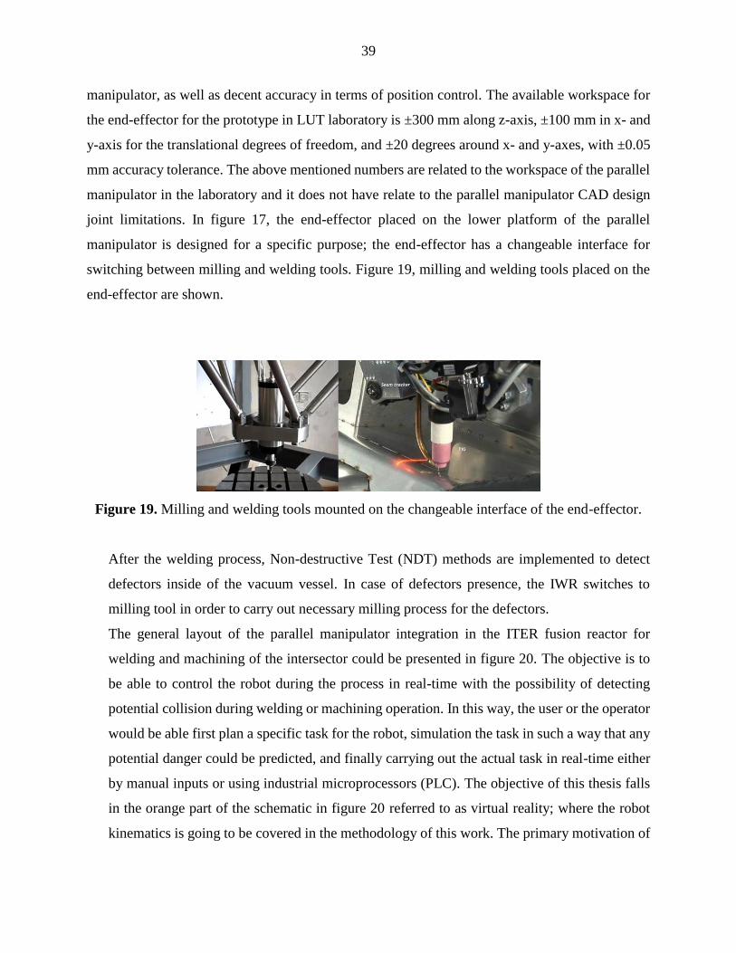
joint limitations. In figure 17, the end-effector placed on the lower platform of the parallel
manipulator is designed for a specific purpose; the end-effector has a changeable interface for
switching between milling and welding tools. Figure 19, milling and welding tools placed on the
end-effector are shown.
Figure 19. Milling and welding tools mounted on the changeable interface of the end-effector.
After the welding process, Non-destructive Test (NDT) methods are implemented to detect
defectors inside of the vacuum vessel. In case of defectors presence, the IWR switches to
milling tool in order to carry out necessary milling process for the defectors.
The general layout of the parallel manipulator integration in the ITER fusion reactor for
welding and machining of the intersector could be presented in figure 20. The objective is to
be able to control the robot during the process in real-time with the possibility of detecting
potential collision during welding or machining operation. In this way, the user or the operator
would be able first plan a specific task for the robot, simulation the task in such a way that any
potential danger could be predicted, and finally carrying out the actual task in real-time either
by manual inputs or using industrial microprocessors (PLC). The objective of this thesis falls
in the orange part of the schematic in figure 20 referred to as virtual reality; where the robot
kinematics is going to be covered in the methodology of this work. The primary motivation of
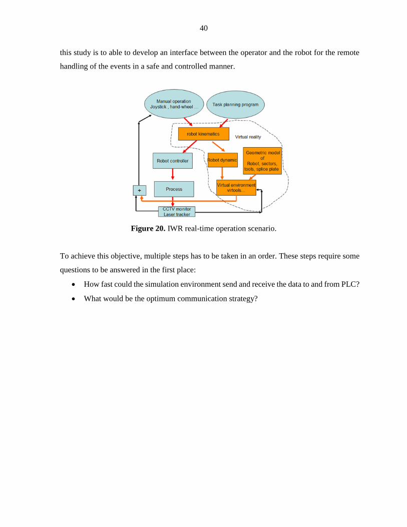
40
this study is to able to develop an interface between the operator and the robot for the remote
handling of the events in a safe and controlled manner.
Figure 20. IWR real-time operation scenario.
To achieve this objective, multiple steps has to be taken in an order. These steps require some
questions to be answered in the first place:
How fast could the simulation environment send and receive the data to and from PLC?
What would be the optimum communication strategy?
41
3. METHODOLOGY
In this chapter, the real-time simulation of the robot is performed and the steps are explained in
the order. These steps include preparing the mathematical model of the system based on inverse
kinematics, model loading and importing CAD files from SolidWorks, simulating the robot in the
offline mode, stablishing online connection, and finally real-time simulation of the robot.
Firstly, the simulation environment shell has to be chosen, which has to meet a certain requirement;
the only criterion is that the environment has to be available to the public free of charge for usage
and its source code should be available as well for further development purposes. This criterion
leaves two different approaches available: either building the environment from scratch or using
already available open-source programs. Considering the scope of this thesis, building an
environment from scratch is not feasible, as it requires sophisticated knowledge of computer
science and 3D graphics experience. In order to build such environments, one could choose from
different options available such as OpenGL or Direct3D, which are graphical libraries available
on the windows. The downside with this approach is that unless the user is not sophisticated
enough in working with 3D graphics and computer programming, the prepared environment might
not be optimized enough to meet the required speed for real-time simulation. The other option is
using open-source software that already have graphical aspects built in for the user. Commercial
software such as SolidWorks, SimMechanics (MATLAB/Simulink), Adams, and other options
cannot be used, as they are not open-source meaning that user must buy the license to use the
software and the source code is not provided as well. Therefore, the best options are using game
engines. Game engines such as Unreal Engine and Unity are geared for game development
purposes, which require very high speeds, very good graphics, and real-time communication of
multiple clients with each other as well as with a server. One game engine is Unity; unity source
code is not fully available for development purposes and the interface language is C#, and it does
not need any license for usage by the user. Unreal Engine has its source code available on the
GitHub and users can easily access that for development purposes, and the interface language is
C++. Another important difference between Unreal Engine and Unity is that Unity does not have
plugins and one must write a custom plugin for that, but Unreal Engine has multiple plugin types,
which eases the communication for the user. After the environment is chosen, the mathematical
42
model of the robot has to be derived; there are two ways with which this robot can be simulated;
either with forward kinematics or with inverse kinematics. Parallel robots have very complicated
forward kinematics and deriving their mathematical model using forward kinematics required
optimization algorithms. Inverse kinematics of parallel robots, on the other hand, is straightforward
and it only requires mathematical operations on geometrical vectors of the mechanism. Which is
covered in methodology chapter. The next step is to import the CAD models of the robot parts
from SolidWroks into Unreal Engine. The model loading is also another important step in this
project as it shows the accuracy of the loaded model. In low-level graphics such as OpenGL and
Direct3D, one should write a custom code for model loading along with using some related
libraries; referring to the same optimization issue discussed earlier, a custom application is not
necessarily an optimal one if it is not organized and compiled by sophisticated users. Model
loading consist of many different parts: lighting, shaders, textures, materials, colors, and vertices.
Each of these features have their own functions that has to be implemented. However, in Game
engines, these are implemented as regular functionalities. The next step is simulation the imported
model with all the components in off-line mode; this means that as there is no physical constrains
in the intended simulation, these joints must be simulated based on mathematical equations and
the results should resemble the degrees of freedom as the original model with physical constrains.
After the off-line simulation, the online communication should be established and for that, the
connection options should be chosen based on the Unreal Engine functionalities.
As the simulation of robot in this thesis does not involve any physics, the mathematical equations
of the manipulator has to be derived based on literature. Two approaches that could be
implemented are forward and inverse kinematics. The forward kinematics of parallel manipulators
are very complicated and they require optimization algorithms with iterative approaches. On the
other hand, the inverse kinematics of parallel manipulators is very easy and straightforward. The
schematic of the studied parallel manipulator with 6 actuators could be simplified as depicted in
the figure 14 [30].
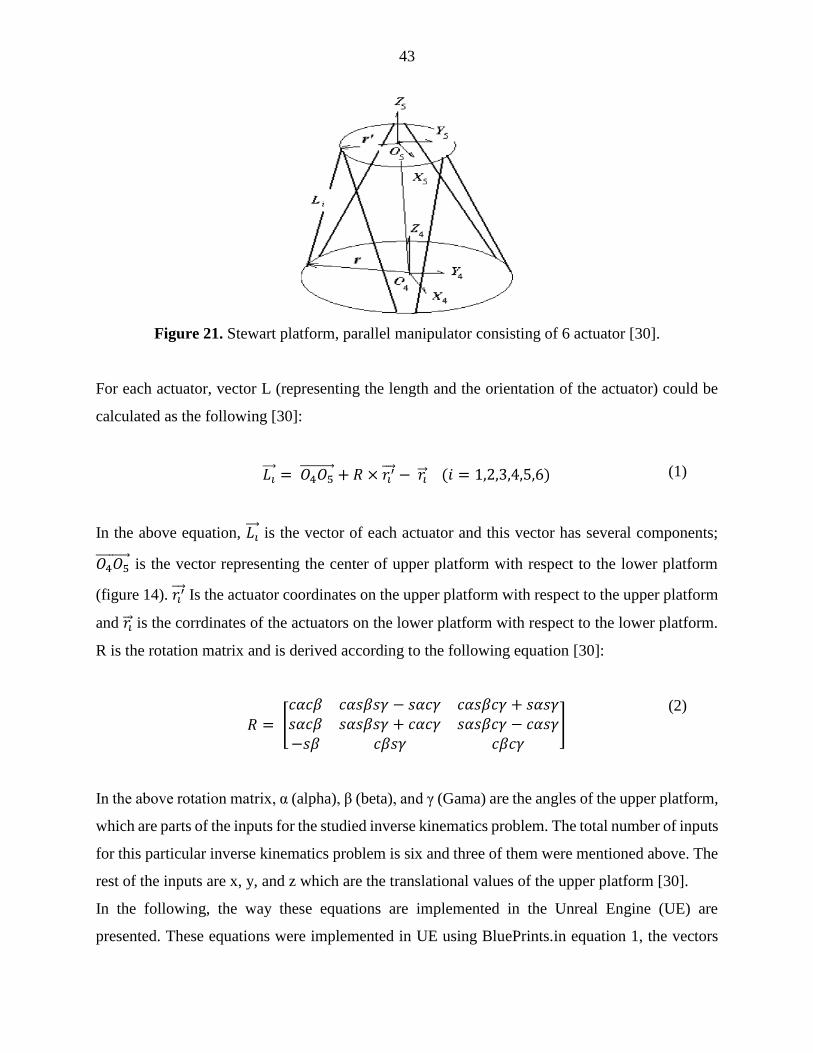
43
Figure 21. Stewart platform, parallel manipulator consisting of 6 actuator [30].
For each actuator, vector L (representing the length and the orientation of the actuator) could be
calculated as the following [30]:
𝐿𝑖 = 𝑂4𝑂5
+ 𝑅 × 𝑟𝑖′ − 𝑟𝑖 (𝑖 = 1,2,3,4,5,6) (1)
In the above equation, 𝐿𝑖 is the vector of each actuator and this vector has several components;
𝑂4𝑂5 is the vector representing the center of upper platform with respect to the lower platform
(figure 14). 𝑟𝑖′ Is the actuator coordinates on the upper platform with respect to the upper platform
and 𝑟𝑖 is the corrdinates of the actuators on the lower platform with respect to the lower platform.
R is the rotation matrix and is derived according to the following equation [30]:
𝑅 = [
𝑐𝛼𝑐𝛽 𝑐𝛼𝑠𝛽𝑠𝛾 − 𝑠𝛼𝑐𝛾 𝑐𝛼𝑠𝛽𝑐𝛾 + 𝑠𝛼𝑠𝛾𝑠𝛼𝑐𝛽 𝑠𝛼𝑠𝛽𝑠𝛾 + 𝑐𝛼𝑐𝛾 𝑠𝛼𝑠𝛽𝑐𝛾 − 𝑐𝛼𝑠𝛾−𝑠𝛽 𝑐𝛽𝑠𝛾 𝑐𝛽𝑐𝛾
] (2)
In the above rotation matrix, α (alpha), β (beta), and γ (Gama) are the angles of the upper platform,
which are parts of the inputs for the studied inverse kinematics problem. The total number of inputs
for this particular inverse kinematics problem is six and three of them were mentioned above. The
rest of the inputs are x, y, and z which are the translational values of the upper platform [30].
In the following, the way these equations are implemented in the Unreal Engine (UE) are
presented. These equations were implemented in UE using BluePrints.in equation 1, the vectors
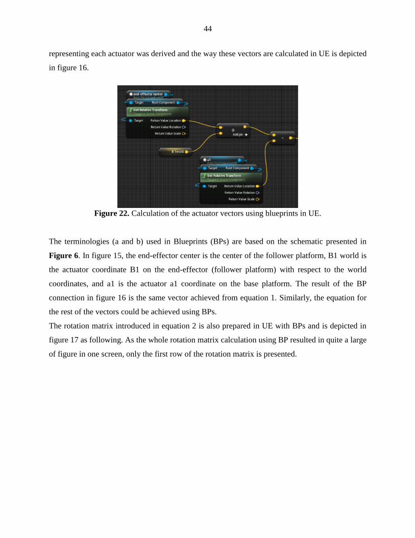
44
representing each actuator was derived and the way these vectors are calculated in UE is depicted
in figure 16.
Figure 22. Calculation of the actuator vectors using blueprints in UE.
The terminologies (a and b) used in Blueprints (BPs) are based on the schematic presented in
Figure 6. In figure 15, the end-effector center is the center of the follower platform, B1 world is
the actuator coordinate B1 on the end-effector (follower platform) with respect to the world
coordinates, and a1 is the actuator a1 coordinate on the base platform. The result of the BP
connection in figure 16 is the same vector achieved from equation 1. Similarly, the equation for
the rest of the vectors could be achieved using BPs.
The rotation matrix introduced in equation 2 is also prepared in UE with BPs and is depicted in
figure 17 as following. As the whole rotation matrix calculation using BP resulted in quite a large
of figure in one screen, only the first row of the rotation matrix is presented.
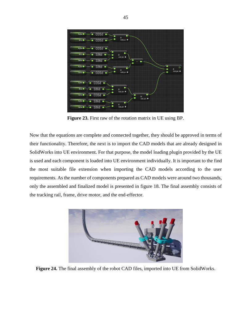
45
Figure 23. First raw of the rotation matrix in UE using BP.
Now that the equations are complete and connected together, they should be approved in terms of
their functionality. Therefore, the next is to import the CAD models that are already designed in
SolidWorks into UE environment. For that purpose, the model loading plugin provided by the UE
is used and each component is loaded into UE environment individually. It is important to the find
the most suitable file extension when importing the CAD models according to the user
requirements. As the number of components prepared as CAD models were around two thousands,
only the assembled and finalized model is presented in figure 18. The final assembly consists of
the tracking rail, frame, drive motor, and the end-effector.
Figure 24. The final assembly of the robot CAD files, imported into UE from SolidWorks.
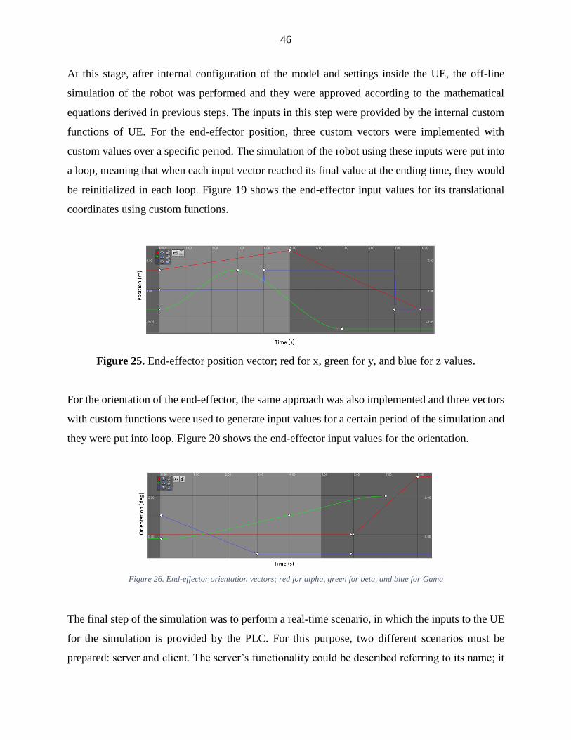
46
At this stage, after internal configuration of the model and settings inside the UE, the off-line
simulation of the robot was performed and they were approved according to the mathematical
equations derived in previous steps. The inputs in this step were provided by the internal custom
functions of UE. For the end-effector position, three custom vectors were implemented with
custom values over a specific period. The simulation of the robot using these inputs were put into
a loop, meaning that when each input vector reached its final value at the ending time, they would
be reinitialized in each loop. Figure 19 shows the end-effector input values for its translational
coordinates using custom functions.
Figure 25. End-effector position vector; red for x, green for y, and blue for z values.
For the orientation of the end-effector, the same approach was also implemented and three vectors
with custom functions were used to generate input values for a certain period of the simulation and
they were put into loop. Figure 20 shows the end-effector input values for the orientation.
Figure 26. End-effector orientation vectors; red for alpha, green for beta, and blue for Gama
The final step of the simulation was to perform a real-time scenario, in which the inputs to the UE
for the simulation is provided by the PLC. For this purpose, two different scenarios must be
prepared: server and client. The server’s functionality could be described referring to its name; it
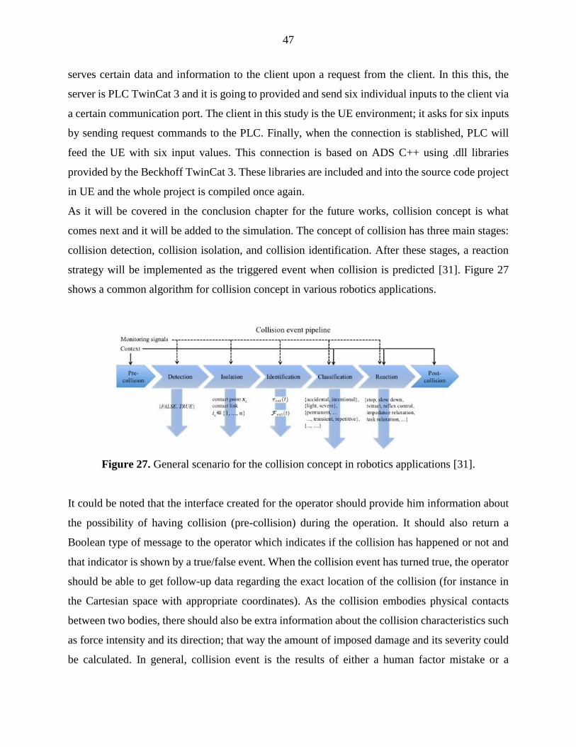
47
serves certain data and information to the client upon a request from the client. In this this, the
server is PLC TwinCat 3 and it is going to provided and send six individual inputs to the client via
a certain communication port. The client in this study is the UE environment; it asks for six inputs
by sending request commands to the PLC. Finally, when the connection is stablished, PLC will
feed the UE with six input values. This connection is based on ADS C++ using .dll libraries
provided by the Beckhoff TwinCat 3. These libraries are included and into the source code project
in UE and the whole project is compiled once again.
As it will be covered in the conclusion chapter for the future works, collision concept is what
comes next and it will be added to the simulation. The concept of collision has three main stages:
collision detection, collision isolation, and collision identification. After these stages, a reaction
strategy will be implemented as the triggered event when collision is predicted [31]. Figure 27
shows a common algorithm for collision concept in various robotics applications.
Figure 27. General scenario for the collision concept in robotics applications [31].
It could be noted that the interface created for the operator should provide him information about
the possibility of having collision (pre-collision) during the operation. It should also return a
Boolean type of message to the operator which indicates if the collision has happened or not and
that indicator is shown by a true/false event. When the collision event has turned true, the operator
should be able to get follow-up data regarding the exact location of the collision (for instance in
the Cartesian space with appropriate coordinates). As the collision embodies physical contacts
between two bodies, there should also be extra information about the collision characteristics such
as force intensity and its direction; that way the amount of imposed damage and its severity could
be calculated. In general, collision event is the results of either a human factor mistake or a
48
malfunction in the mechanics of the system; it could also be said interpreted that the collision could
be either intentional or unintentional. In case it was an intentional incident, the training process of
the operator could be reviewed to see if there were any flaws present in the process. On the other
hand, if it was a system malfunction, then the system has to be checked thoroughly to identify the
source of failure. At the time of collision, the triggered event or the reaction of the system is
important; the simplest way is that the robot stops and the system could shut down. That way, the
operator has to time to make the decision about what to do next. Finally, the last stage would be to
check condition after the collision and when a decision has been made. At this stage, there could
either be another collision possibility or it could be sage to continue the operation [31].
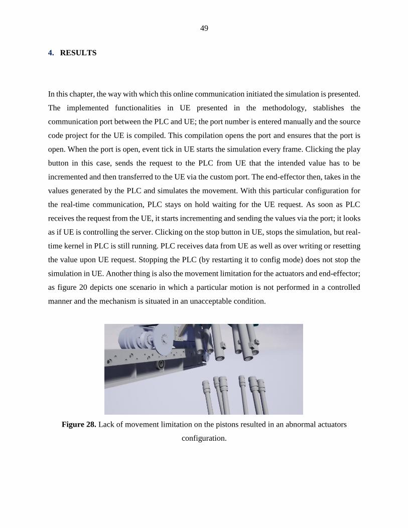
49
4. RESULTS
In this chapter, the way with which this online communication initiated the simulation is presented.
The implemented functionalities in UE presented in the methodology, stablishes the
communication port between the PLC and UE; the port number is entered manually and the source
code project for the UE is compiled. This compilation opens the port and ensures that the port is
open. When the port is open, event tick in UE starts the simulation every frame. Clicking the play
button in this case, sends the request to the PLC from UE that the intended value has to be
incremented and then transferred to the UE via the custom port. The end-effector then, takes in the
values generated by the PLC and simulates the movement. With this particular configuration for
the real-time communication, PLC stays on hold waiting for the UE request. As soon as PLC
receives the request from the UE, it starts incrementing and sending the values via the port; it looks
as if UE is controlling the server. Clicking on the stop button in UE, stops the simulation, but real-
time kernel in PLC is still running. PLC receives data from UE as well as over writing or resetting
the value upon UE request. Stopping the PLC (by restarting it to config mode) does not stop the
simulation in UE. Another thing is also the movement limitation for the actuators and end-effector;
as figure 20 depicts one scenario in which a particular motion is not performed in a controlled
manner and the mechanism is situated in an unacceptable condition.
Figure 28. Lack of movement limitation on the pistons resulted in an abnormal actuators
configuration.
50
5. DISCUSSION
The presented results in the previous chapter are discussed in this section and their reasons are also
analyzed.
The first issue to address is the relationship between PLC as the server and UE as the client.
Compiling the project before simulation automatically establishes and opens the port. This is the
desired objective, as it has to be a separate sequence. Stopping the simulation from inside of UE
does not stop the real-time kernel in PLC and that is because of the fact that PLC is not controlled
or interrupted by the UE as client; in other words, stopping the simulation from within UE, does
not send any command (request) to the PLC regarding its run, which is favorable as PLC has to be
running independently and this approves the logical relationship between the server and the client.
Stopping PLC or restarting it to config mode does not stop the simulation in UE and that is because
the real-time kernel in PLC is not linked to the UE. Typically, the communication should be
reversed; PLC should run and stop the simulation. In other words, PLC should have the capability
to control the simulation, but at the same time, it should be waiting for the clients requests as well.
At some point in the simulation, the joints on the either side of the actuators orientate themselves
in unusual ways and pistons as well move completely out of cylinders or go through the other way.
This is because the fact that there was no limitation considered for the robot mechanism in the
design process. There could be two solutions for this scenario; one would be to adjust the
limitations visually, which is a tedious task to do, and if successful, it only makes the simulation
look good and it does not guarantee the proper robot behavior. The second solution would be to
apply these joint constrains in the design mode based on the actual test bench available in the
laboratory, which is the proper way as this real-time simulation is meant to be compared to the
actual laboratory test.
51
6. CONCLUSION
The purpose of the thesis work was to establish a real-time 3D simulation environment for the
simulation of the parallel manipulator of the fusion reactor that is controlled by aa PLC. The
outcome of the study with proposed methodology was development of 3D simulation environment
with a real-time communication port with PLC.
To answer the first research question raised in the study, the question is repeated here:
How fast could the simulation environment send and receive the data to and from PLC? By running
the PLC on one side and having the simulation in UE on the other side, the simulation begins
instantly and it exactly follows the values being sent from the PLC into the simulation. The second
question was: What would be the optimum communication strategy? Among the available
communication means and mechanisms by the PLC TwinCat 3, only ADS C++ could be
implemented in this thesis as it uses precompiled libraries provided by the Beckhoff. This type of
communication is not internet based, but pointer based, which makes the communication more
secure and stable; there is always possibility of loss of data in internet based connections, as the
client and server are not communicating with each other directly.
This research only prepared and environment for the real-time 3D simulation of a specific parallel
manipulator. Further research and investigation would be to implement an algorithm with which
the behavior of the robot could be predicted, as the actual robot inside the reactor could not be seen
because of the harsh environmental aspects such as hot and pressured atmosphere as well as lack
of light. Apart from that, different algorithms regarding the collision detection could be
implemented to have more sophisticated approaches in terms of collision between two objects.
52
REFERENCES
[1] Carlo Damiani, Alessandro Tesini, Satoshi Kakudate. The Remote Handling Systems for
ITER; 2010.
[2] Chanyang Li. DESIGN AND ANALYSIS OF ROBOT FOR THE MAINTENANCE OF
DIVERTOR IN DEMO FUSION REACTOR. Master's thesis, School of energy systems,
Lappeenranta University of Technolgy 2017.
[3] Willard L V Pollard, inventor. Position Controlling Apparatus.
[4] V. E. Gough and S. G. Whitehall, editor. Universal Tyre Test Machine. 9th; 1962.
[5] Stewart D. A Platform with Six Degrees of Freedom. Proceedings of the Institution of
Mechanical Engineers 1965; 180(1): 371–86.
[6] wang Y, Pessi P, Wu H, Handroos H. Accuracy analysis of hybrid parallel robot for the
assembling of ITER. Fusion Engineering and Design 2009; 84(7-11): 1964–8
[https://doi.org/10.1016/j.fusengdes.2008.11.072]
[7] Johari NAM, Haron H, Jaya ASM. Robotic modeling and simulation of palletizer robot using
Workspace5. In: Robotic modeling and simulation of palletizer robot using Workspace5; 2007
- 2007. IEEE; 217–22.
[8] Ulgen OM, Coffman G, Rohrer M, Shore J, Sly D, Wood D. Increasing the power and value
of manufacturing simulation via collaboration with other analytical tools: a panel discussion.
In: Increasing the power and value of manufacturing simulation via collaboration with other
analytical tools: a panel discussion; 1999. IEEE; 749–53.
[9] Wolfe R. Bringing the introductory computer graphics course into the 21st century. Computers
& Graphics 2000; 24(1): 151–5.
[10] Luna FD. Introduction to 3D game programming with DirectX 10. Jones & Bartlett
Publishers 2008.
[11] Hanwell MD, Martin KM, Chaudhary A, Avila LS. The Visualization Toolkit
(VTK): Rewriting the rendering code for modern graphics cards. SoftwareX 2015; 1: 9–12.
[12] Schroeder WJ, Lorensen B, Martin K. The visualization toolkit: an object-oriented
approach to 3D graphics. Kitware 2004.
[13] Moreland K, Sewell C, Usher W, et al. Vtk-m: Accelerating the visualization toolkit
for massively threaded architectures. IEEE computer graphics and applications 2016; 36(3):
48–58.
53
[14] Martin K, Hoffman B. Mastering CMake: a cross-platform build system. Kitware
2010.
[15] Avila LS, Barre S, Blue R, et al. The VTK User’s Guide. Kitware New York 2010.
[16] Tracy S, Reindell P. CryENGINE 3 Game Development: Beginner’s Guide. Packt
Publishing Ltd 2012.
[17] Xie J. Research on key technologies base Unity3D game engine. In: Research on key
technologies base Unity3D game engine; 2012 - 2012. IEEE; 695–9.
[18] Shaoqiang Y, Zhong L, Xingshan L. Modeling and simulation of robot based on
Matlab/SimMechanics. In: Modeling and simulation of robot based on Matlab/SimMechanics;
2008 - 2008. IEEE; 161–5.
[19] Quigley M, Conley K, Gerkey B, et al. ROS: an open-source Robot Operating
System. In: ROS: an open-source Robot Operating System; 2009; 5.
[20] Aitken JM, Veres SM, Judge M. Adaptation of system configuration under the robot
operating system. IFAC Proceedings Volumes 2014; 47(3): 4484–92.
[21] Tardioli D, Parasuraman R, Ögren P. Pound: A multi-master ROS node for reducing
delay and jitter in wireless multi-robot networks. Robotics and Autonomous Systems 2018.
[22] Adams - The Multibody Dynamics Simulation Solution; 2018 [cited 2018 November
22] Available from: URL: http://www.mscsoftware.com/product/adams.
[23] Mitra AC, Fernandes E, Nawpute K, Sheth S, Kadam V, Chikhale SJ. Development
and Validation of a Simulation Model of Automotive Suspension System using MSC-
ADAMS. Materials Today: Proceedings 2018; 5(2): 4327–34.
[24] Badr WS, Fanni M, Abdel-Rahman AK, Rasoul SA. Dynamic simulation and
optimization of rhombic drive Stirling engine using MSC ADAMS software. Procedia
Technology 2016; 22: 754–61.
[25] Sapietova A, Bukovan J, Sapieta M, Jakubovicova L. Analysis and implementation
of input load effects on an air compressor piston in MSC. ADAMS. Procedia Engineering
2017; 177: 554–61.
[26] Sanders A. An Introduction to Unreal Engine 4. AK Peters/CRC Press 2016.
[27] Busby J, Parrish Z, Wilson J. Mastering unreal technology, volume i: Introduction
to level design with unreal engine 3. Pearson Education 2009.
54
[28] Alphonsus ER, Abdullah MO. A review on the applications of programmable logic
controllers (PLCs). Renewable and Sustainable Energy Reviews 2016; 60: 1185–205.
[29] BECKHOFF. Manual TC3 C++ TwinCAT 3; 2018 [cited 2018 November 29]
Available from: URL:
http://download.beckhoff.com/download/document/automation/twincat3/TC1300_C_EN.pdf
.
[30] Pessi P, Wu H, Handroos H, others. Accuracy analysis of hybrid parallel robot for
the assembling of ITER. Fusion Engineering and Design 2009; 84(7-11): 1964–8.
[31] Haddadin S, Luca A de, Albu-Schäffer A. Robot collisions: A survey on detection,
isolation, and identification. IEEE Transactions on Robotics 2017; 33(6): 1292–312.