Embed Size (px)
Citation preview

125
Figure 56. Map of the neuronal functional cluster identified during seizures.
3D reconstruction of the neuronal clusters identified through correlation analysis (see Data analysis) during epileptic activity recording. Overlay of 30 fluorescence imaged planes of the same 4 dpf zebrafish larva seen in Figure 52 and the widespread neuronal cluster identified based on strong pixel correlation after 50 minutes exposure to PTZ.
Development of optical methods for real-time whole-brain functional imaging of zebrafish neuronal activity
LAPO
TU
RR
INI
FIRENZEUNIVERSITY
PRESS
LAPO TURRINI
2019Scientif ica
pr
em
io
T
es
i
do
TT
or
aT
o
fir
en
ze
un
iver
siT
y p
res
s –
un
iver
siTà d
egLi s
Tu
di d
i fir
en
ze
Developm
ent of optical methods for real-tim
e whole-brain functional im
aging of zebrafish neuronal activity
FUP

premio tesi di dottorato
ISSN 2612-8039 (PRINT) | ISSN 2612-8020 (ONLINE)
– 85 –

PREMIO TESI DI DOTTORATO
Commissione giudicatrice, anno 2019
Vincenzo Varano, Presidente della Commissione
Tito Arecchi, Area ScientificaAldo Bompani, Area delle Scienze SocialiMario Caciagli, Area delle Scienze SocialiFranco Cambi, Area UmanisticaGiancarlo Garfagnini, Area UmanisticaRoberto Genesio, Area TecnologicaFlavio Moroni, Area BiomedicaAdolfo Pazzagli, Area BiomedicaGiuliano Pinto, Area UmanisticaVincenzo Schettino, Area ScientificaMaria Chiara Torricelli, Area TecnologicaLuca Uzielli, Area TecnologicaGraziella Vescovini, Area Umanistica
2

Lapo Turrini
Development of optical methods for real-time whole-brain functional imaging of
zebrafish neuronal activity
Firenze University Press2020

Graphic design: Alberto Pizarro Fernández, Lettera Meccanica SRLs
***FUP Best Practice in Scholarly Publishing (DOI 10.36253/fup_best_practice)All publications are submitted to an external refereeing process under the responsibility of the FUP Editorial Board and the Scientific Boards of the series. The works published are evaluated and approved by the Editorial Board of the publishing house, and must be compliant with the Peer review policy, the Open Access, Copyright and Licensing policy and the Publication Ethics and Complaint policy. Firenze University Press Editorial Board M. Garzaniti (Editor-in-Chief), M.E. Alberti, M. Boddi, A. Bucelli, R. Casalbuoni, F. Ciampi, A. Dolfi, R. Ferrise, P. Guarnieri, R. Lanfredini, P. Lo Nostro, G. Mari, A. Mariani, P.M. Mariano, S. Marinai, R. Minuti, P. Nanni, A. Orlandi, A. Perulli, G. Pratesi, O. Roselli.
The online digital edition is published in Open Access on www.fupress.com.Content license: the present work is released under Creative Commons Attribution 4.0 International license (CC BY 4.0: http://creativecommons.org/licenses/by/4.0/legalcode). This license allows you to share any part of the work by any means and format, modify it for any purpose, including commercial, as long as appropriate credit is given to the author, any changes made to the work are indicated and a URL link is provided to the license. Metadata license: all the metadata are released under the Public Domain Dedication license (CC0 1.0 Universal: https://creativecommons.org/publicdomain/zero/1.0/legalcode).© 2020 Author(s)Published by Firenze University Press
Firenze University PressUniversità degli Studi di Firenzevia Cittadella, 7, 50144 Firenze, Italywww.fupress.com
This book is printed on acid-free paperPrinted in Italy
Development of optical methods for real-time whole-brain functional imaging of zebrafish neuronal activity / Lapo Turrini. – Firenze : Firenze University Press, 2020.(Premio Tesi di Dottorato ; 85)
https://www.fupress.com/isbn/9788855180702
ISSN 2612-8039 (print) ISSN 2612-8020 (online) ISBN 978-88-5518-069-6 (print) ISBN 978-88-5518-070-2 (PDF) ISBN 978-88-5518-071-9 (XML) DOI 10.36253/978-88-5518-070-2
5
‘[...] But the fool on the hill sees the sun going down and the eyes in his head
see the world spinning round [...]’
from The Fool on the Hill John Lennon and Paul McCartney, 1967
4

5
‘[...] But the fool on the hill sees the sun going down and the eyes in his head
see the world spinning round [...]’
from The Fool on the Hill John Lennon and Paul McCartney, 1967

66 7
Table of Contents
Part I Introduction
Chapter 1 Motivation: the brain challenge 13
Chapter 2 The neuron 17
Chapter 3 Fluorescence theory 21 3.1 Two-photon excitation fluorescence 24
Chapter 4 The Green Fluorescent Protein 27
Chapter 5 Genetically encoded Ca2+ indicators 31 5.1 GCaMP6s 35
Chapter 6 Fluorescence microscopy 37 6.1 Wide-field fluorescence microscopy 38 6.2 Light-sheet fluorescence microscopy 39
6.2.1 Light-sheet fluorescence microscopy: drawbacks and solutions 44 6.2.1.1 Bessel beams illumination 45
Chapter 7 Zebrafish in neurosciences 47 7.1 Zebrafish and epilepsy 54
Part II Methods
Chapter 8
6

7
Table of Contents
Part I Introduction
Chapter 1 Motivation: the brain challenge 13
Chapter 2 The neuron 17
Chapter 3 Fluorescence theory 21 3.1 Two-photon excitation fluorescence 24
Chapter 4 The Green Fluorescent Protein 27
Chapter 5 Genetically encoded Ca2+ indicators 31 5.1 GCaMP6s 35
Chapter 6 Fluorescence microscopy 37 6.1 Wide-field fluorescence microscopy 38 6.2 Light-sheet fluorescence microscopy 39
6.2.1 Light-sheet fluorescence microscopy: drawbacks and solutions 44 6.2.1.1 Bessel beams illumination 45
Chapter 7 Zebrafish in neurosciences 47 7.1 Zebrafish and epilepsy 54
Part II Methods
Chapter 8 Lapo Turrini, Development of optical methods for real-time whole-brain functional imaging of zebrafish neuronal activity, © 2020 Author(s), content CC BY 4.0 International, metadata CC0 1.0 Universal, published by Firenze University Press (www.fupress.com), ISSN 2612-8020 (online), ISBN 978-88-5518-070-2 (PDF), DOI 10.36253/978-88-5518-070-2

Real-time whole-brain functional imaging of zebrafish neuronal activity
9
14.2.2 Bessel beam illumination light-sheet microscopy 3D optical mapping analysis 87
14.3 Two-photon light-sheet fluorescence microscopy whole-brain measurements analysis 88
Part III Results
Chapter 15 Optical mapping of zebrafish neuronal activity in a pharmacological model of epilepsy 93 15.1 GCaMP6s optical measurements show basal and PTZ-altered activity in the zebrafish brain 93 15.2 GCaMP6s fluorescence measurements are sensitive to different PTZ concentrations 95 15.3 Correlation analysis among brain regions and locomotor activity 97 15.4 High-throughput combined fluorescence and behavioural recordings 102
Chapter 16 Bessel beam illumination as a means to reduce artefacts in quantitative functional studies using light-sheet microscopy 105 16.1 Streaking artefacts obscure microscopic features of interest 105 16.2 Flickering quantification 108 16.3 Impact of flickering on neuronal activity measurements 110 16.4 Flickering artefacts mask neuronal correlations 111
Chapter 17 3D optical mapping of zebrafish neuronal activity with single cell resolution by Bessel beam illumination light-sheet microscopy 115
Chapter 18 Fast whole-brain functional imaging by two-photon light-sheet fluorescence microscopy 119
Part IV Discussion
Chapter 19 Optical mapping of neuronal activity during PTZ-induced seizures 131
Chapter 20 Bessel beam illumination reduces haemodynamic artefacts in functional light-sheet fluorescence microscopy 135
8
Generation of the GCaMP6s transgenic zebrafish line 59 8.1 Amplification of plasmid tol2-elavl3:H2B-GCaMP6s 60
8.1.1 Bacterial transformation with tol2-elavl3:H2B-GCaMP6s plasmid 60 8.1.2 tol2-elavl3:H2B-GCaMP6s plasmid extraction 60
8.2 In vitro transcription of tol2 plasmid 61 8.3 Microinjection 61 8.4 Transgenic line selection 62
Chapter 9 Microscopes 65 9.1 Wide-field fluorescence microscope 65 9.2 Dual-illumination light-sheet fluorescence microscope 66 9.3 Two-photon light-sheet microscope 68
Chapter 10 Zebrafish husbandry 71
Chapter 11 Sample mounting 73 11.1 Wide-field fluorescence microscopy imaging 73 11.2 Dual-illumination light-sheet fluorescence microscopy imaging 73 11.3 Two-photon light-sheet fluorescence microscopy imaging 74
Chapter 12 Chemicals preparation 77
Chapter 13 Optical measurements 79 13.1 Wide-field optical mapping measurements 79
13.1.1 Combined electrographic and fluorescence recordings 79 13.1.2 High-throughput measurements 79
13.2 Dual-illumination light-sheet fluorescence microscopy measurements 80 13.3 Two-photon light-sheet fluorescence microscopy measurements 81
Chapter 14 Data analysis 83 14.1 Wide-field optical mapping measurements analysis 83
14.1.1 High-throughput measurements analysis 84 14.2 Dual-illumination light-sheet fluorescence microscopy measurements analysis 84
14.2.1 Haemodynamic artefacts measurements analysis 84
7
Table of Contents
Part I Introduction
Chapter 1 Motivation: the brain challenge 13
Chapter 2 The neuron 17
Chapter 3 Fluorescence theory 21 3.1 Two-photon excitation fluorescence 24
Chapter 4 The Green Fluorescent Protein 27
Chapter 5 Genetically encoded Ca2+ indicators 31 5.1 GCaMP6s 35
Chapter 6 Fluorescence microscopy 37 6.1 Wide-field fluorescence microscopy 38 6.2 Light-sheet fluorescence microscopy 39
6.2.1 Light-sheet fluorescence microscopy: drawbacks and solutions 44 6.2.1.1 Bessel beams illumination 45
Chapter 7 Zebrafish in neurosciences 47 7.1 Zebrafish and epilepsy 54
Part II Methods
Chapter 8
8
Generation of the GCaMP6s transgenic zebrafish line 59 8.1 Amplification of plasmid tol2-elavl3:H2B-GCaMP6s 60
8.1.1 Bacterial transformation with tol2-elavl3:H2B-GCaMP6s plasmid 60 8.1.2 tol2-elavl3:H2B-GCaMP6s plasmid extraction 60
8.2 In vitro transcription of tol2 plasmid 61 8.3 Microinjection 61 8.4 Transgenic line selection 62
Chapter 9 Microscopes 65 9.1 Wide-field fluorescence microscope 65 9.2 Dual-illumination light-sheet fluorescence microscope 66 9.3 Two-photon light-sheet microscope 68
Chapter 10 Zebrafish husbandry 71
Chapter 11 Sample mounting 73 11.1 Wide-field fluorescence microscopy imaging 73 11.2 Dual-illumination light-sheet fluorescence microscopy imaging 73 11.3 Two-photon light-sheet fluorescence microscopy imaging 74
Chapter 12 Chemicals preparation 77
Chapter 13 Optical measurements 79 13.1 Wide-field optical mapping measurements 79
13.1.1 Combined electrographic and fluorescence recordings 79 13.1.2 High-throughput measurements 79
13.2 Dual-illumination light-sheet fluorescence microscopy measurements 80 13.3 Two-photon light-sheet fluorescence microscopy measurements 81
Chapter 14 Data analysis 83 14.1 Wide-field optical mapping measurements analysis 83
14.1.1 High-throughput measurements analysis 84 14.2 Dual-illumination light-sheet fluorescence microscopy measurements analysis 84
14.2.1 Haemodynamic artefacts measurements analysis 84 8

Lapo Turrini
9
14.2.2 Bessel beam illumination light-sheet microscopy 3D optical mapping analysis 87
14.3 Two-photon light-sheet fluorescence microscopy whole-brain measurements analysis 88
Part III Results
Chapter 15 Optical mapping of zebrafish neuronal activity in a pharmacological model of epilepsy 93 15.1 GCaMP6s optical measurements show basal and PTZ-altered activity in the zebrafish brain 93 15.2 GCaMP6s fluorescence measurements are sensitive to different PTZ concentrations 95 15.3 Correlation analysis among brain regions and locomotor activity 97 15.4 High-throughput combined fluorescence and behavioural recordings 102
Chapter 16 Bessel beam illumination as a means to reduce artefacts in quantitative functional studies using light-sheet microscopy 105 16.1 Streaking artefacts obscure microscopic features of interest 105 16.2 Flickering quantification 108 16.3 Impact of flickering on neuronal activity measurements 110 16.4 Flickering artefacts mask neuronal correlations 111
Chapter 17 3D optical mapping of zebrafish neuronal activity with single cell resolution by Bessel beam illumination light-sheet microscopy 115
Chapter 18 Fast whole-brain functional imaging by two-photon light-sheet fluorescence microscopy 119
Part IV Discussion
Chapter 19 Optical mapping of neuronal activity during PTZ-induced seizures 131
Chapter 20 Bessel beam illumination reduces haemodynamic artefacts in functional light-sheet fluorescence microscopy 135
14.2.2 Bessel beam illumination light-sheet microscopy 3D optical mapping analysis 87
14.3 Two-photon light-sheet fluorescence microscopy whole-brain measurements analysis 88
Chapter 15 Optical mapping of zebrafish neuronal activity in a pharmacological model of epilepsy 9315.1 GCaMP6s optical measurements show basal and PTZ-altered activity
in the zebrafish brain 93
Chapter 17 3D optical mapping of zebrafish neuronal activity with single cell resolution by Bessel beam illumination light-sheet microscopy 115
Chapter 18 Fast whole-brain functional imaging by two-photon light-sheet fluorescence microscopy 119
8
Generation of the GCaMP6s transgenic zebrafish line 59 8.1 Amplification of plasmid tol2-elavl3:H2B-GCaMP6s 60
8.1.1 Bacterial transformation with tol2-elavl3:H2B-GCaMP6s plasmid 60 8.1.2 tol2-elavl3:H2B-GCaMP6s plasmid extraction 60
8.2 In vitro transcription of tol2 plasmid 61 8.3 Microinjection 61 8.4 Transgenic line selection 62
Chapter 9 Microscopes 65 9.1 Wide-field fluorescence microscope 65 9.2 Dual-illumination light-sheet fluorescence microscope 66 9.3 Two-photon light-sheet microscope 68
Chapter 10 Zebrafish husbandry 71
Chapter 11 Sample mounting 73 11.1 Wide-field fluorescence microscopy imaging 73 11.2 Dual-illumination light-sheet fluorescence microscopy imaging 73 11.3 Two-photon light-sheet fluorescence microscopy imaging 74
Chapter 12 Chemicals preparation 77
Chapter 13 Optical measurements 79 13.1 Wide-field optical mapping measurements 79
13.1.1 Combined electrographic and fluorescence recordings 79 13.1.2 High-throughput measurements 79
13.2 Dual-illumination light-sheet fluorescence microscopy measurements 80 13.3 Two-photon light-sheet fluorescence microscopy measurements 81
Chapter 14 Data analysis 83 14.1 Wide-field optical mapping measurements analysis 83
14.1.1 High-throughput measurements analysis 84 14.2 Dual-illumination light-sheet fluorescence microscopy measurements analysis 84
14.2.1 Haemodynamic artefacts measurements analysis 84
7
Table of Contents
Part I Introduction
Chapter 1 Motivation: the brain challenge 13
Chapter 2 The neuron 17
Chapter 3 Fluorescence theory 21 3.1 Two-photon excitation fluorescence 24
Chapter 4 The Green Fluorescent Protein 27
Chapter 5 Genetically encoded Ca2+ indicators 31 5.1 GCaMP6s 35
Chapter 6 Fluorescence microscopy 37 6.1 Wide-field fluorescence microscopy 38 6.2 Light-sheet fluorescence microscopy 39
6.2.1 Light-sheet fluorescence microscopy: drawbacks and solutions 44 6.2.1.1 Bessel beams illumination 45
Chapter 7 Zebrafish in neurosciences 47 7.1 Zebrafish and epilepsy 54
Part II Methods
Chapter 8
14.2 Dual-illumination light-sheet fluorescence microscopy measurements analysis 84
8
Generation of the GCaMP6s transgenic zebrafish line 59 8.1 Amplification of plasmid tol2-elavl3:H2B-GCaMP6s 60
8.1.1 Bacterial transformation with tol2-elavl3:H2B-GCaMP6s plasmid 60 8.1.2 tol2-elavl3:H2B-GCaMP6s plasmid extraction 60
8.2 In vitro transcription of tol2 plasmid 61 8.3 Microinjection 61 8.4 Transgenic line selection 62
Chapter 9 Microscopes 65 9.1 Wide-field fluorescence microscope 65 9.2 Dual-illumination light-sheet fluorescence microscope 66 9.3 Two-photon light-sheet microscope 68
Chapter 10 Zebrafish husbandry 71
Chapter 11 Sample mounting 73 11.1 Wide-field fluorescence microscopy imaging 73 11.2 Dual-illumination light-sheet fluorescence microscopy imaging 73 11.3 Two-photon light-sheet fluorescence microscopy imaging 74
Chapter 12 Chemicals preparation 77
Chapter 13 Optical measurements 79 13.1 Wide-field optical mapping measurements 79
13.1.1 Combined electrographic and fluorescence recordings 79 13.1.2 High-throughput measurements 79
13.2 Dual-illumination light-sheet fluorescence microscopy measurements 80 13.3 Two-photon light-sheet fluorescence microscopy measurements 81
Chapter 14 Data analysis 83 14.1 Wide-field optical mapping measurements analysis 83
14.1.1 High-throughput measurements analysis 84 14.2 Dual-illumination light-sheet fluorescence microscopy measurements analysis 84
14.2.1 Haemodynamic artefacts measurements analysis 84 9

Real-time whole-brain functional imaging of zebrafish neuronal activity
10
10
Chapter 21 3D mapping of zebrafish neuronal activity by Bessel beam illumination light-sheet fluorescence microscopy 139
Chapter 22 141 Whole-brain neuronal dynamics by two-photon light-sheet fluorescence microscopy 141
Part V Future directions 143
Part VI Appendices
Appendix A 149
Appendix B 175
Bibliography 181
List of publications 193
Acknowledgements 195
11
Part I
Introduction
Chapter 21 3D mapping of zebrafish neuronal activity by Bessel beam illumination lightsheet fluorescence microscopy 139
Chapter 20 Bessel beam illumination reduces haemodynamic artefacts in functional lightsheet fluorescence microscopy 135
10

10
Chapter 21 3D mapping of zebrafish neuronal activity by Bessel beam illumination light-sheet fluorescence microscopy 139
Chapter 22 141 Whole-brain neuronal dynamics by two-photon light-sheet fluorescence microscopy 141
Part V Future directions 143
Part VI Appendices
Appendix A 149
Appendix B 175
Bibliography 181
List of publications 193
Acknowledgements 195
11
Part I
Introduction
Lapo Turrini, Development of optical methods for real-time whole-brain functional imaging of zebrafish neuronal activity, © 2020 Author(s), content CC BY 4.0 International, metadata CC0 1.0 Universal, published by Firenze University Press (www.fupress.com), ISSN 2612-8020 (online), ISBN 978-88-5518-070-2 (PDF), DOI 10.36253/978-88-5518-070-2

13
Chapter 1 Motivation: the brain challenge
The huge variety of human behaviours relies on an elaborate array of sensory receptors connected to an extraordinarily plastic organ, the brain, which actively organizes incoming sensory signals. Perception inputs are in part stored in memory for future reference, and in part converted into immediate behavioural responses. All these processes are managed by a network of interconnected neurons, which are the structural and functional units of the nervous system. Starting from embryonic neuronal progenitor cells which, through millions of years of evolution, have been equipped with the potency to produce every neuron in the nervous system, the adult human brain counts approximately 1011 neurons and as many non-neural cells (Azevedo et al., 2009). This enormous number of cells takes part in constituting circuits with precise functions, in a network that is thought to count more than 1015 synapses (Pakkenberg et al., 2003). The complexity of this system arises not only from the number of elements constituting it but also from their diversity, both in terms of shapes and functions. In fact, neurons of the human brain can be classified, according to gene expression profiling, in up to 104 different cell sub-types (Muotri and Gage, 2006), spanning from elongated retinal cone photoreceptors involved in visual perception, to arborized cerebellar Purkinje cells coordinating motor function, to the hypothalamic osmoreceptor neurons secreting antidiuretic hormone (ADH), to cite just a few. This extraordinary diversity exists even between cells within the same neuronal subtype. Indeed, even neurons with similar morphology can differ in important molecular details (e.g. expression of different combination of membrane ion channels, providing neurons with diverse excitation thresholds and/or distinctive firing patterns), highlighting the importance of single neurons in the network. How and when the outstanding neuronal diversity is generated in the course of neurogenesis, remains however still unclear. Since during embryonic neurogenesis, proliferative precursor neuroblasts migrate to form the adult grey matter and in this process only 15-40% of post migratory cells survive (Finlay and Slattery, 1983;Ferrer et al., 1992), it has been hypothesized that this putative selection process could be responsible for the generation of neuronal diversity (Oppenheim, 1991), through a DNA recombination similar to that seen in the immune system with V(D)J mechanism (Jones and Gellert, 2004). In addition to this process, has been demonstrated the existence of activity-dependent neuronal diversity in postmitotic neurons driven by environmental stimuli that dynamically refine neuronal networks, as it happens, for example, in hippocampal “place cells” (Burgess and O'Keefe, 2003). Yet, to make things even more complex, both neurons and their connections are modified by
12

13
Chapter 1 Motivation: the brain challenge
The huge variety of human behaviours relies on an elaborate array of sensory receptors connected to an extraordinarily plastic organ, the brain, which actively organizes incoming sensory signals. Perception inputs are in part stored in memory for future reference, and in part converted into immediate behavioural responses. All these processes are managed by a network of interconnected neurons, which are the structural and functional units of the nervous system. Starting from embryonic neuronal progenitor cells which, through millions of years of evolution, have been equipped with the potency to produce every neuron in the nervous system, the adult human brain counts approximately 1011 neurons and as many non-neural cells (Azevedo et al., 2009). This enormous number of cells takes part in constituting circuits with precise functions, in a network that is thought to count more than 1015 synapses (Pakkenberg et al., 2003). The complexity of this system arises not only from the number of elements constituting it but also from their diversity, both in terms of shapes and functions. In fact, neurons of the human brain can be classified, according to gene expression profiling, in up to 104 different cell sub-types (Muotri and Gage, 2006), spanning from elongated retinal cone photoreceptors involved in visual perception, to arborized cerebellar Purkinje cells coordinating motor function, to the hypothalamic osmoreceptor neurons secreting antidiuretic hormone (ADH), to cite just a few. This extraordinary diversity exists even between cells within the same neuronal subtype. Indeed, even neurons with similar morphology can differ in important molecular details (e.g. expression of different combination of membrane ion channels, providing neurons with diverse excitation thresholds and/or distinctive firing patterns), highlighting the importance of single neurons in the network. How and when the outstanding neuronal diversity is generated in the course of neurogenesis, remains however still unclear. Since during embryonic neurogenesis, proliferative precursor neuroblasts migrate to form the adult grey matter and in this process only 15-40% of post migratory cells survive (Finlay and Slattery, 1983;Ferrer et al., 1992), it has been hypothesized that this putative selection process could be responsible for the generation of neuronal diversity (Oppenheim, 1991), through a DNA recombination similar to that seen in the immune system with V(D)J mechanism (Jones and Gellert, 2004). In addition to this process, has been demonstrated the existence of activity-dependent neuronal diversity in postmitotic neurons driven by environmental stimuli that dynamically refine neuronal networks, as it happens, for example, in hippocampal “place cells” (Burgess and O'Keefe, 2003). Yet, to make things even more complex, both neurons and their connections are modified by
Lapo Turrini, Development of optical methods for real-time whole-brain functional imaging of zebrafish neuronal activity, © 2020 Author(s), content CC BY 4.0 International, metadata CC0 1.0 Universal, published by Firenze University Press (www.fupress.com), ISSN 2612-8020 (online), ISBN 978-88-5518-070-2 (PDF), DOI 10.36253/978-88-5518-070-2
Real-time whole-brain functional imaging of zebrafish neuronal activity
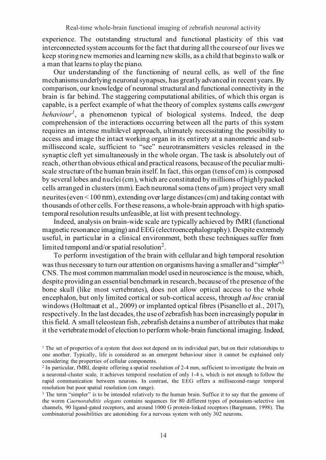
14
experience. The outstanding structural and functional plasticity of this vast interconnected system accounts for the fact that during all the course of our lives we keep storing new memories and learning new skills, as a child that begins to walk or a man that learns to play the piano.
Our understanding of the functioning of neural cells, as well of the fine mechanisms underlying neuronal synapses, has greatly advanced in recent years. By comparison, our knowledge of neuronal structural and functional connectivity in the brain is far behind. The staggering computational abilities, of which this organ is capable, is a perfect example of what the theory of complex systems calls emergent behaviour1, a phenomenon typical of biological systems. Indeed, the deep comprehension of the interactions occurring between all the parts of this system requires an intense multilevel approach, ultimately necessitating the possibility to access and image the intact working organ in its entirety at a nanometric and sub-millisecond scale, sufficient to “see” neurotransmitters vesicles released in the synaptic cleft yet simultaneously in the whole organ. The task is absolutely out of reach, other than obvious ethical and practical reasons, because of the peculiar multi-scale structure of the human brain itself. In fact, this organ (tens of cm) is composed by several lobes and nuclei (cm), which are constituted by millions of highly packed cells arranged in clusters (mm). Each neuronal soma (tens of µm) project very small neurites (even < 100 nm), extending over large distances (cm) and taking contact with thousands of other cells. For these reasons, a whole-brain approach with high spatio-temporal resolution results unfeasible, at list with present technology.
Indeed, analysis on brain-wide scale are typically achieved by fMRI (functional magnetic resonance imaging) and EEG (electroencephalography). Despite extremely useful, in particular in a clinical environment, both these techniques suffer from limited temporal and/or spatial resolution2.
To perform investigation of the brain with cellular and high temporal resolution was thus necessary to turn our attention on organisms having a smaller and “simpler”3 CNS. The most common mammalian model used in neuroscience is the mouse, which, despite providing an essential benchmark in research, because of the presence of the bone skull (like most vertebrates), does not allow optical access to the whole encephalon, but only limited cortical or sub-cortical access, through ad hoc cranial windows (Holtmaat et al., 2009) or implanted optical fibres (Pisanello et al., 2017), respectively. In the last decades, the use of zebrafish has been increasingly popular in this field. A small teleostean fish, zebrafish detains a number of attributes that make it the vertebrate model of election to perform whole-brain functional imaging. Indeed,
1 The set of properties of a system that does not depend on its individual part, but on their relationships to one another. Typically, life is considered as an emergent behaviour since it cannot be explained only considering the properties of cellular components. 2 In particular, fMRI, despite offering a spatial resolution of 2-4 mm, sufficient to investigate the brain on a neuronal-cluster scale, it achieves temporal resolution of only 1-4 s, which is not enough to follow the rapid communication between neurons. In contrast, the EEG offers a millisecond-range temporal resolution but poor spatial resolution (cm range). 3 The term “simpler” is to be intended relatively to the human brain. Suffice it to say that the genome of the worm Caernorabditis elegans contains sequences for 80 different types of potassium-selective ion channels, 90 ligand-gated receptors, and around 1000 G protein-linked receptors (Bargmann, 1998). The combinatorial possibilities are astonishing for a nervous system with only 302 neurons.
15
currently available state-of-the-art fluorescence microscopes (Ahrens et al., 2013;Tomer et al., 2015) allow for real-time optical access of the whole translucent zebrafish larva brain (~105 neurons) expressing fluorescent neuronal activity indicators. The synergy between technological improvement, fluorescent biosensors development and this transparent organism opened the way to the unprecedented non-invasive in vivo functional investigation of a vertebrate brain in its entirety.
14

Lapo Turrini
14
experience. The outstanding structural and functional plasticity of this vast interconnected system accounts for the fact that during all the course of our lives we keep storing new memories and learning new skills, as a child that begins to walk or a man that learns to play the piano.
Our understanding of the functioning of neural cells, as well of the fine mechanisms underlying neuronal synapses, has greatly advanced in recent years. By comparison, our knowledge of neuronal structural and functional connectivity in the brain is far behind. The staggering computational abilities, of which this organ is capable, is a perfect example of what the theory of complex systems calls emergent behaviour1, a phenomenon typical of biological systems. Indeed, the deep comprehension of the interactions occurring between all the parts of this system requires an intense multilevel approach, ultimately necessitating the possibility to access and image the intact working organ in its entirety at a nanometric and sub-millisecond scale, sufficient to “see” neurotransmitters vesicles released in the synaptic cleft yet simultaneously in the whole organ. The task is absolutely out of reach, other than obvious ethical and practical reasons, because of the peculiar multi-scale structure of the human brain itself. In fact, this organ (tens of cm) is composed by several lobes and nuclei (cm), which are constituted by millions of highly packed cells arranged in clusters (mm). Each neuronal soma (tens of µm) project very small neurites (even < 100 nm), extending over large distances (cm) and taking contact with thousands of other cells. For these reasons, a whole-brain approach with high spatio-temporal resolution results unfeasible, at list with present technology.
Indeed, analysis on brain-wide scale are typically achieved by fMRI (functional magnetic resonance imaging) and EEG (electroencephalography). Despite extremely useful, in particular in a clinical environment, both these techniques suffer from limited temporal and/or spatial resolution2.
To perform investigation of the brain with cellular and high temporal resolution was thus necessary to turn our attention on organisms having a smaller and “simpler”3 CNS. The most common mammalian model used in neuroscience is the mouse, which, despite providing an essential benchmark in research, because of the presence of the bone skull (like most vertebrates), does not allow optical access to the whole encephalon, but only limited cortical or sub-cortical access, through ad hoc cranial windows (Holtmaat et al., 2009) or implanted optical fibres (Pisanello et al., 2017), respectively. In the last decades, the use of zebrafish has been increasingly popular in this field. A small teleostean fish, zebrafish detains a number of attributes that make it the vertebrate model of election to perform whole-brain functional imaging. Indeed,
1 The set of properties of a system that does not depend on its individual part, but on their relationships to one another. Typically, life is considered as an emergent behaviour since it cannot be explained only considering the properties of cellular components. 2 In particular, fMRI, despite offering a spatial resolution of 2-4 mm, sufficient to investigate the brain on a neuronal-cluster scale, it achieves temporal resolution of only 1-4 s, which is not enough to follow the rapid communication between neurons. In contrast, the EEG offers a millisecond-range temporal resolution but poor spatial resolution (cm range). 3 The term “simpler” is to be intended relatively to the human brain. Suffice it to say that the genome of the worm Caernorabditis elegans contains sequences for 80 different types of potassium-selective ion channels, 90 ligand-gated receptors, and around 1000 G protein-linked receptors (Bargmann, 1998). The combinatorial possibilities are astonishing for a nervous system with only 302 neurons.
15
currently available state-of-the-art fluorescence microscopes (Ahrens et al., 2013;Tomer et al., 2015) allow for real-time optical access of the whole translucent zebrafish larva brain (~105 neurons) expressing fluorescent neuronal activity indicators. The synergy between technological improvement, fluorescent biosensors development and this transparent organism opened the way to the unprecedented non-invasive in vivo functional investigation of a vertebrate brain in its entirety.
15

17
Chapter 2 The neuron
The neuron is the structural and functional unit of the nervous system. A typical neuron can be divided in four morphologically defined regions: cell body, dendrites, axon and presynaptic terminals (Fig.1). The cell body (soma) contains the nucleus and is the metabolic centre of the cell. From the soma, two different kinds of processes originate: several short dendrites and one long axon. Dendrites form branches and are the main tool for receiving incoming signals from other nerve cells.
The axon instead, is typically longer than dendrites and carries signals to other neurons. Large axons are typically wrapped in an insulating sheath of a lipid substance, myelin. The sheath is interrupted at regular intervals, every 1-2 mm, by gaps of bare axon membrane approximately 1 µm wide, the nodes of Ranvier.
Figure 1. Schematic structure of a neuron.
From the cell body, which contains the nucleus, originate two different kinds of processes: dendrites (usually several), used by the neuron to receive signals from other cells, and axons (typically one), used to send signals to other cells. Dendrites are the postsynaptic elements of the synapse, whereas axons represent the presynaptic part. From (Kandel, 2013).
16

17
Chapter 2 The neuron
The neuron is the structural and functional unit of the nervous system. A typical neuron can be divided in four morphologically defined regions: cell body, dendrites, axon and presynaptic terminals (Fig.1). The cell body (soma) contains the nucleus and is the metabolic centre of the cell. From the soma, two different kinds of processes originate: several short dendrites and one long axon. Dendrites form branches and are the main tool for receiving incoming signals from other nerve cells.
The axon instead, is typically longer than dendrites and carries signals to other neurons. Large axons are typically wrapped in an insulating sheath of a lipid substance, myelin. The sheath is interrupted at regular intervals, every 1-2 mm, by gaps of bare axon membrane approximately 1 µm wide, the nodes of Ranvier.
Figure 1. Schematic structure of a neuron.
From the cell body, which contains the nucleus, originate two different kinds of processes: dendrites (usually several), used by the neuron to receive signals from other cells, and axons (typically one), used to send signals to other cells. Dendrites are the postsynaptic elements of the synapse, whereas axons represent the presynaptic part. From (Kandel, 2013).
Lapo Turrini, Development of optical methods for real-time whole-brain functional imaging of zebrafish neuronal activity, © 2020 Author(s), content CC BY 4.0 International, metadata CC0 1.0 Universal, published by Firenze University Press (www.fupress.com), ISSN 2612-8020 (online), ISBN 978-88-5518-070-2 (PDF), DOI 10.36253/978-88-5518-070-2

Real-time whole-brain functional imaging of zebrafish neuronal activity
18
The comprehensive structure of the neuron did not become clear until late 19th century, when Camillo Golgi and Santiago Ramón y Cajal began to use the “reazione nera” (black reaction) introduced by the former in 1883 (Golgi, 1885). Still used today, this silver impregnation method has two advantages. First, in a random manner, that to present day is still not fully understood, silver nitrate solution stains only about 1% of the cells in any particular brain region, making it possible to examine a single neuron in isolation from its neighbours. Second, stained neurons are delineated in their entirety, including cell body, axon, and full dendritic tree. Applying Golgi’s method, Ramón y Cajal performed a meticulous work: he examined the structure of neurons in almost every region of the nervous system, described different classes of nerve cells and mapped the precise connections between many of them (Ramòn y Cajal, 1917) (Fig.2).
From a functional point of view, neurons communicate through action potentials, which are transient electrical signals originating at the hillock, the initial segment of the axon, and propagating along all the process length. The lipid bilayer constituting cell plasma membrane is impermeable to ions and thus represent an insulator separating two conducting solutions, the cytoplasm and the extracellular fluid. Ions can cross this lipid barrier only by passing through ion channels present in the cell membrane. When a cell is at rest, passive ionic fluxes into and out of the cell are balanced, so that the charge separation across the membrane remains constant and membrane potential is maintained at its resting value. In this scenario, the dynamic equilibrium potential E for any X ion can be calculated using the Nernst equation (Nernst, 1888):
𝐸𝐸𝑋𝑋 = 𝑅𝑅𝑅𝑅𝑧𝑧𝑧𝑧 𝑙𝑙𝑙𝑙 [𝑋𝑋]𝑜𝑜
[𝑋𝑋]𝑖𝑖
where R is the gas constant, T the temperature expressed in Kelvin degrees, z the
valence of the ion, F the Faraday constant, and [X]o and [X]i are the concentrations of the ion outside and inside the cell.
The resting membrane potential Vm, representing the electrical potential (voltage) across the membrane due to charge separation, can be obtained calculating Goldman equation (Goldman D.E., 1943) for the ion species involved:
Figure 2. Reazione nera.
Hand drawing of a pyramidal neuron of the cerebral cortex stained with Golgi’s reazione nera, by Santiago Ramón y Cajal (1852-1934).
19
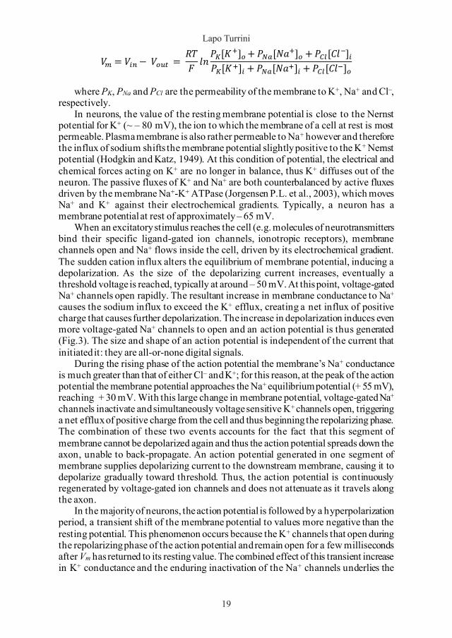
𝑉𝑉𝑚𝑚 = 𝑉𝑉𝑖𝑖𝑖𝑖 − 𝑉𝑉𝑜𝑜𝑜𝑜𝑜𝑜 = 𝑅𝑅𝑅𝑅𝐹𝐹 𝑙𝑙𝑙𝑙 𝑃𝑃𝐾𝐾[𝐾𝐾+]𝑜𝑜 + 𝑃𝑃𝑁𝑁𝑁𝑁[𝑁𝑁𝑁𝑁+]𝑜𝑜 + 𝑃𝑃𝐶𝐶𝐶𝐶[𝐶𝐶𝑙𝑙−]𝑖𝑖
𝑃𝑃𝐾𝐾[𝐾𝐾+]𝑖𝑖 + 𝑃𝑃𝑁𝑁𝑁𝑁[𝑁𝑁𝑁𝑁+]𝑖𝑖 + 𝑃𝑃𝐶𝐶𝐶𝐶[𝐶𝐶𝑙𝑙−]𝑜𝑜
where PK, PNa and PCl are the permeability of the membrane to K+, Na+ and Cl–,
respectively. In neurons, the value of the resting membrane potential is close to the Nernst
potential for K+ (~ – 80 mV), the ion to which the membrane of a cell at rest is most permeable. Plasma membrane is also rather permeable to Na+ however and therefore the influx of sodium shifts the membrane potential slightly positive to the K+ Nernst potential (Hodgkin and Katz, 1949). At this condition of potential, the electrical and chemical forces acting on K+ are no longer in balance, thus K+ diffuses out of the neuron. The passive fluxes of K+ and Na+ are both counterbalanced by active fluxes driven by the membrane Na+-K+ ATPase (Jorgensen P.L. et al., 2003), which moves Na+ and K+ against their electrochemical gradients. Typically, a neuron has a membrane potential at rest of approximately – 65 mV.
When an excitatory stimulus reaches the cell (e.g. molecules of neurotransmitters bind their specific ligand-gated ion channels, ionotropic receptors), membrane channels open and Na+ flows inside the cell, driven by its electrochemical gradient. The sudden cation influx alters the equilibrium of membrane potential, inducing a depolarization. As the size of the depolarizing current increases, eventually a threshold voltage is reached, typically at around – 50 mV. At this point, voltage-gated Na+ channels open rapidly. The resultant increase in membrane conductance to Na+ causes the sodium influx to exceed the K+ efflux, creating a net influx of positive charge that causes further depolarization. The increase in depolarization induces even more voltage-gated Na+ channels to open and an action potential is thus generated (Fig.3). The size and shape of an action potential is independent of the current that initiated it: they are all-or-none digital signals.
During the rising phase of the action potential the membrane’s Na+ conductance is much greater than that of either Cl– and K+; for this reason, at the peak of the action potential the membrane potential approaches the Na+ equilibrium potential (+ 55 mV), reaching + 30 mV. With this large change in membrane potential, voltage-gated Na+ channels inactivate and simultaneously voltage sensitive K+ channels open, triggering a net efflux of positive charge from the cell and thus beginning the repolarizing phase. The combination of these two events accounts for the fact that this segment of membrane cannot be depolarized again and thus the action potential spreads down the axon, unable to back-propagate. An action potential generated in one segment of membrane supplies depolarizing current to the downstream membrane, causing it to depolarize gradually toward threshold. Thus, the action potential is continuously regenerated by voltage-gated ion channels and does not attenuate as it travels along the axon.
In the majority of neurons, the action potential is followed by a hyperpolarization period, a transient shift of the membrane potential to values more negative than the resting potential. This phenomenon occurs because the K+ channels that open during the repolarizing phase of the action potential and remain open for a few milliseconds after Vm has returned to its resting value. The combined effect of this transient increase in K+ conductance and the enduring inactivation of the Na+ channels underlies the
18
Lapo Turrini
18
The comprehensive structure of the neuron did not become clear until late 19th century, when Camillo Golgi and Santiago Ramón y Cajal began to use the “reazione nera” (black reaction) introduced by the former in 1883 (Golgi, 1885). Still used today, this silver impregnation method has two advantages. First, in a random manner, that to present day is still not fully understood, silver nitrate solution stains only about 1% of the cells in any particular brain region, making it possible to examine a single neuron in isolation from its neighbours. Second, stained neurons are delineated in their entirety, including cell body, axon, and full dendritic tree. Applying Golgi’s method, Ramón y Cajal performed a meticulous work: he examined the structure of neurons in almost every region of the nervous system, described different classes of nerve cells and mapped the precise connections between many of them (Ramòn y Cajal, 1917) (Fig.2).
From a functional point of view, neurons communicate through action potentials, which are transient electrical signals originating at the hillock, the initial segment of the axon, and propagating along all the process length. The lipid bilayer constituting cell plasma membrane is impermeable to ions and thus represent an insulator separating two conducting solutions, the cytoplasm and the extracellular fluid. Ions can cross this lipid barrier only by passing through ion channels present in the cell membrane. When a cell is at rest, passive ionic fluxes into and out of the cell are balanced, so that the charge separation across the membrane remains constant and membrane potential is maintained at its resting value. In this scenario, the dynamic equilibrium potential E for any X ion can be calculated using the Nernst equation (Nernst, 1888):
𝐸𝐸𝑋𝑋 = 𝑅𝑅𝑅𝑅𝑧𝑧𝑧𝑧 𝑙𝑙𝑙𝑙 [𝑋𝑋]𝑜𝑜
[𝑋𝑋]𝑖𝑖
where R is the gas constant, T the temperature expressed in Kelvin degrees, z the
valence of the ion, F the Faraday constant, and [X]o and [X]i are the concentrations of the ion outside and inside the cell.
The resting membrane potential Vm, representing the electrical potential (voltage) across the membrane due to charge separation, can be obtained calculating Goldman equation (Goldman D.E., 1943) for the ion species involved:
Figure 2. Reazione nera.
Hand drawing of a pyramidal neuron of the cerebral cortex stained with Golgi’s reazione nera, by Santiago Ramón y Cajal (1852-1934).
19
𝑉𝑉𝑚𝑚 = 𝑉𝑉𝑖𝑖𝑖𝑖 − 𝑉𝑉𝑜𝑜𝑜𝑜𝑜𝑜 = 𝑅𝑅𝑅𝑅𝐹𝐹 𝑙𝑙𝑙𝑙
𝑃𝑃𝐾𝐾[𝐾𝐾+]𝑜𝑜 + 𝑃𝑃𝑁𝑁𝑁𝑁[𝑁𝑁𝑁𝑁+]𝑜𝑜 + 𝑃𝑃𝐶𝐶𝐶𝐶[𝐶𝐶𝑙𝑙−]𝑖𝑖𝑃𝑃𝐾𝐾[𝐾𝐾+]𝑖𝑖 + 𝑃𝑃𝑁𝑁𝑁𝑁[𝑁𝑁𝑁𝑁+]𝑖𝑖 + 𝑃𝑃𝐶𝐶𝐶𝐶[𝐶𝐶𝑙𝑙−]𝑜𝑜
where PK, PNa and PCl are the permeability of the membrane to K+, Na+ and Cl–,
respectively. In neurons, the value of the resting membrane potential is close to the Nernst
potential for K+ (~ – 80 mV), the ion to which the membrane of a cell at rest is most permeable. Plasma membrane is also rather permeable to Na+ however and therefore the influx of sodium shifts the membrane potential slightly positive to the K+ Nernst potential (Hodgkin and Katz, 1949). At this condition of potential, the electrical and chemical forces acting on K+ are no longer in balance, thus K+ diffuses out of the neuron. The passive fluxes of K+ and Na+ are both counterbalanced by active fluxes driven by the membrane Na+-K+ ATPase (Jorgensen P.L. et al., 2003), which moves Na+ and K+ against their electrochemical gradients. Typically, a neuron has a membrane potential at rest of approximately – 65 mV.
When an excitatory stimulus reaches the cell (e.g. molecules of neurotransmitters bind their specific ligand-gated ion channels, ionotropic receptors), membrane channels open and Na+ flows inside the cell, driven by its electrochemical gradient. The sudden cation influx alters the equilibrium of membrane potential, inducing a depolarization. As the size of the depolarizing current increases, eventually a threshold voltage is reached, typically at around – 50 mV. At this point, voltage-gated Na+ channels open rapidly. The resultant increase in membrane conductance to Na+ causes the sodium influx to exceed the K+ efflux, creating a net influx of positive charge that causes further depolarization. The increase in depolarization induces even more voltage-gated Na+ channels to open and an action potential is thus generated (Fig.3). The size and shape of an action potential is independent of the current that initiated it: they are all-or-none digital signals.
During the rising phase of the action potential the membrane’s Na+ conductance is much greater than that of either Cl– and K+; for this reason, at the peak of the action potential the membrane potential approaches the Na+ equilibrium potential (+ 55 mV), reaching + 30 mV. With this large change in membrane potential, voltage-gated Na+ channels inactivate and simultaneously voltage sensitive K+ channels open, triggering a net efflux of positive charge from the cell and thus beginning the repolarizing phase. The combination of these two events accounts for the fact that this segment of membrane cannot be depolarized again and thus the action potential spreads down the axon, unable to back-propagate. An action potential generated in one segment of membrane supplies depolarizing current to the downstream membrane, causing it to depolarize gradually toward threshold. Thus, the action potential is continuously regenerated by voltage-gated ion channels and does not attenuate as it travels along the axon.
In the majority of neurons, the action potential is followed by a hyperpolarization period, a transient shift of the membrane potential to values more negative than the resting potential. This phenomenon occurs because the K+ channels that open during the repolarizing phase of the action potential and remain open for a few milliseconds after Vm has returned to its resting value. The combined effect of this transient increase in K+ conductance and the enduring inactivation of the Na+ channels underlies the
19

Real-time whole-brain functional imaging of zebrafish neuronal activity
20
absolute refractory period, the short time following an action potential when it is impossible to elicit a new action potential. The refractory period limits the frequency at which a neuron can fire action potentials, and thus limits the information-carrying capacity of the axon.
The functional design of neurons is determined by two opposing requirements. First, they have to be small, so that large numbers can fit into the brain and spinal cord, in order to maximize the computing power of the nervous system. Second, they also have to conduct signals very rapidly, to maximize the ability of the organism to respond to environmental changes. Neurons are indeed small, but they consist of a thin membrane surrounded by two conducting media and thus they have high capacitance. Moreover, the electrical signals flow through a relatively poor conductor, a thin column of cytoplasm. These two factors combine to slow down the conduction of voltage signals.
Figure 3. Action potential and underlying ionic conductances.
The sequential opening of voltage-gated Na+ and K+ produce the typical shape of the action potential. From (Kandel, 2013).
Two adaptive strategies have evolved to increase the propagation of the action potential. One is an increase in the diameter of the axon, which reduces the axial resistance inside the process (to the extreme of the giant axon of the squid, which can reach 1 mm in diameter). The second strategy is the wrapping of a myelin sheath around the axon. This process is functionally equivalent to increase the thickness of the axonal membrane and thus increases the electrical resistance of the membrane. To prevent the action potential from running out, the small patch of membrane present in each node of Ranvier is rich in voltage-gated Na+ channels and thus can generate an intense depolarizing inward Na+ current that periodically propagates the electric signal. The action potential spreads rapidly along the internode because of the low capacitance in correspondence of the myelin sheath and slows down as it crosses the high-capacitance region of each node. For this reason, the propagation of an action potential in a myelinated axon is termed saltatory conduction.
21
Chapter 3 Fluorescence theory
Fluorescence is a phenomenon consisting in the molecular absorption of electromagnetic radiation (photons) at one wavelength and its re-emission at another, usually longer, wavelength.
The first reported observation of fluorescence was made by Nicolàs Monardes, a Spanish physician and botanist. In 1565, he published the ‘Historia medicinal de las cosas que se traen de nuestras Indias Occidentales’, in which he describes how, under certain conditions of observation, an infusion of Eysenhardtia polystachia, a wood from Mexico, took a peculiar opalescent blue colour4 (Fig.4) (Valeur and Berberan-Santos M.N., 2011). Figure 4. First observation of fluorescence.
Painting representing a cup made of E. polystachia wood and a flask containing its fluorescent solution. In 1565, Nicolàs Monardes described for the first time the phenomenon that, three hundred years later, would have been given the name fluorescence by Sir G.G. Stokes. E. polystachia is a wood from Mexico at that time used to treat kidney diseases (for this reason named lignum nephriticum). This wood, already known to Aztecs, was a scarce and expensive medicine. Monardes in his essay suggests using the opalescent blue colour unleashed by the infusion to detect counterfeited wood (Valeur and Berberan-Santos M.N., 2011). From (Safford, 1915).
4 Lignum nephriticum was a scarce and expensive medicine; therefore, it was of particular interest to detect counterfeited wood. On this respect, in his assay Monardes wrote, “Make sure that the wood renders water bluish, otherwise it is a falsification. Indeed, they now bring another kind of wood that renders the water yellow, but it is not good, only the kind that renders the water bluish is genuine”. This method for the detection of a counterfeited good it is considered the first application of the phenomenon that would be later called fluorescence.
20

20
absolute refractory period, the short time following an action potential when it is impossible to elicit a new action potential. The refractory period limits the frequency at which a neuron can fire action potentials, and thus limits the information-carrying capacity of the axon.
The functional design of neurons is determined by two opposing requirements. First, they have to be small, so that large numbers can fit into the brain and spinal cord, in order to maximize the computing power of the nervous system. Second, they also have to conduct signals very rapidly, to maximize the ability of the organism to respond to environmental changes. Neurons are indeed small, but they consist of a thin membrane surrounded by two conducting media and thus they have high capacitance. Moreover, the electrical signals flow through a relatively poor conductor, a thin column of cytoplasm. These two factors combine to slow down the conduction of voltage signals.
Figure 3. Action potential and underlying ionic conductances.
The sequential opening of voltage-gated Na+ and K+ produce the typical shape of the action potential. From (Kandel, 2013).
Two adaptive strategies have evolved to increase the propagation of the action potential. One is an increase in the diameter of the axon, which reduces the axial resistance inside the process (to the extreme of the giant axon of the squid, which can reach 1 mm in diameter). The second strategy is the wrapping of a myelin sheath around the axon. This process is functionally equivalent to increase the thickness of the axonal membrane and thus increases the electrical resistance of the membrane. To prevent the action potential from running out, the small patch of membrane present in each node of Ranvier is rich in voltage-gated Na+ channels and thus can generate an intense depolarizing inward Na+ current that periodically propagates the electric signal. The action potential spreads rapidly along the internode because of the low capacitance in correspondence of the myelin sheath and slows down as it crosses the high-capacitance region of each node. For this reason, the propagation of an action potential in a myelinated axon is termed saltatory conduction.
21
Chapter 3 Fluorescence theory
Fluorescence is a phenomenon consisting in the molecular absorption of electromagnetic radiation (photons) at one wavelength and its re-emission at another, usually longer, wavelength.
The first reported observation of fluorescence was made by Nicolàs Monardes, a Spanish physician and botanist. In 1565, he published the ‘Historia medicinal de las cosas que se traen de nuestras Indias Occidentales’, in which he describes how, under certain conditions of observation, an infusion of Eysenhardtia polystachia, a wood from Mexico, took a peculiar opalescent blue colour4 (Fig.4) (Valeur and Berberan-Santos M.N., 2011). Figure 4. First observation of fluorescence.
Painting representing a cup made of E. polystachia wood and a flask containing its fluorescent solution. In 1565, Nicolàs Monardes described for the first time the phenomenon that, three hundred years later, would have been given the name fluorescence by Sir G.G. Stokes. E. polystachia is a wood from Mexico at that time used to treat kidney diseases (for this reason named lignum nephriticum). This wood, already known to Aztecs, was a scarce and expensive medicine. Monardes in his essay suggests using the opalescent blue colour unleashed by the infusion to detect counterfeited wood (Valeur and Berberan-Santos M.N., 2011). From (Safford, 1915).
4 Lignum nephriticum was a scarce and expensive medicine; therefore, it was of particular interest to detect counterfeited wood. On this respect, in his assay Monardes wrote, “Make sure that the wood renders water bluish, otherwise it is a falsification. Indeed, they now bring another kind of wood that renders the water yellow, but it is not good, only the kind that renders the water bluish is genuine”. This method for the detection of a counterfeited good it is considered the first application of the phenomenon that would be later called fluorescence. Lapo Turrini, Development of optical methods for real-time whole-brain functional imaging of zebrafish neuronal activity, © 2020 Author(s), content CC BY 4.0 International, metadata CC0 1.0 Universal, published by Firenze University Press (www.fupress.com), ISSN 2612-8020 (online), ISBN 978-88-5518-070-2 (PDF), DOI 10.36253/978-88-5518-070-2

Real-time whole-brain functional imaging of zebrafish neuronal activity
22
This phenomenon is due to the peculiar electronic structure of some molecules, called fluorophores. The molecular transitions underlying the emission of fluorescence are typically illustrated by the Jablonski diagram (Fig.5).
Figure 5. Jablonski's diagram.
The processes occurring in a molecule between the absorption and emission of light are usually illustrated by this kind of diagram, named after Alexander Jablonski, who is regarded as the father of fluorescence spectroscopy. The singlet ground, first and second electronic states of a fluorophore are depicted by S0, S1 and S2, respectively. At each of these electronic energy levels, molecules can exist in a number of vibrational energy levels (0, 1 and 2). hνA, hνF, and hνP represent the molecular absorption of a photon, the emission of a fluorescence photon and the emission of a phosphorescence photon, respectively. T1 indicates the first triplet state. h𝜈𝜈𝐴𝐴
2 represents the almost simultaneous absorption of two photons having each half the energy necessary to induce a single photon excitation. Adapted from (Lakowicz, 2006).
In such diagrams, the energy levels of a molecule are depicted as straight segments, ordered according to energy on the vertical axis and grouped according to the spin state (singlet or triplet) on the horizontal axis. Each electronic energy level (S0, S1, etc.) is split in a manifold of vibrational and rotational states of slightly different energies (for display reason, only vibrational levels are shown in Figure 5). At room temperature, molecules typically lie in the ground state S0. The molecular absorption of light (hνA) can induce an electronic transition (occurring in about 10-15 s), that brings the fluorophore from S0 to some higher vibrational level of either S1 or S2. Molecules rapidly relax to the lowest vibrational level of S1, dissipating energy in a non-radiative way. This process is called internal conversion and generally occurs within 10-12 s or less. After internal conversion, fluorophores return, typically, to the higher vibrational levels of the ground state (in about 10-8 s) with emission of one photon (hνF). This transition is allowed because the electron in the excited orbital is paired (by opposite spin) to the second electron in the ground-state orbital. Examination of the Jablonski diagram (Fig.5) reveals that energy of the emitted radiation (hνF) is typically lower than that of the absorbed one (hνA). Each photon
23
absorbed results in the release of a lower energy (longer wavelength) fluorescence photon. This phenomenon was first described by Sir. G. G. Stokes in his ‘On the change of refrangibility of light’ in 1852 and is named Stokes shift after him. The energy loss between excitation and emission is principally due to the rapid decay to the lowest vibrational level of S1. In this process, part of the energy transferred from the photon to the molecule is dissipated in the form of heat. Furthermore, fluorophores generally decay to higher vibrational levels of S0, resulting in further loss of excitation energy by thermalization of the excess vibrational energy. Molecules in the S1 state have a small probability to undergo a spin conversion to the first triplet state T1, a process called intersystem crossing (ISC). Emission from T1 is termed phosphorescence and is generally shifted to longer wavelengths (lower energy) relative to fluorescence. Transition from T1 to the singlet ground state is highly unlikely (because of unpaired spin), and as a result the lifetime of the triplet state is several orders of magnitude larger (typically, 10-5 to 10-3 s) than that for fluorescence (Lakowicz, 2006). Fluorophores, however, can return to the S0 ground state through interaction with the environment; in particular, from the energy transfer with 3O2 (which is itself a triplet in the ground state), singlet molecular oxygen 1O2 is produced. Moreover, electron transfer can occur from the triplet fluorophore to molecular oxygen, leading to the formation of a superoxide radical O2-. Singlet oxygen and superoxide radical, along with other oxidizing species formed subsequently (HO·, HO2·, HO2-, H2O2), are collectively termed reactive oxygen species (ROS) which can degrade fluorophores and bring them in a non-fluorescent dark state (Ha and Tinnefeld, 2012;Zheng et al., 2014). This phenomenon is known as photobleaching, and accounts for the fact that, even if in principle a fluorophore can cycle between ground and excited states an unlimited number of times, due to environmental interactions fluorescence emission from a single molecule can abruptly cease. When recording the integrated fluorescence emitted by hundreds of thousands of fluorophore molecules, photobleaching consists in a progressive decrease of emitted light, upon constant excitation power.
The spectral properties of fluorophores, in terms of excitation and emission, are generally presented as fluorescence spectra. The fluorescence spectrum of a fluorophore expresses the likelihood that excitation and emission will occur as a function of wavelength (Fig.6). An excitation spectrum is characterized by a maximum that corresponds to the wavelength which most efficiently can excite the fluorophore; light with a wavelength near the excitation maximum can cause excitation too, but less efficiently. The fluorescence emission spectrum has a similar meaning; the fluorescence output of a fluorophore is most likely to occur at a particular wavelength, the emission maximum for that fluorophore. The excited fluorophore can also emit light at wavelength around the emission maximum, however the light will be less intense. As the electronic transitions underlying fluorescence emission typically occur between manifolds and not single states, fluorescence spectra are formed by bands rather than sharp lines. For example, the lowest fluorescence wavelengths registered (highest energy emitted) are typically due to the emission from the lowest vibrational level of the excited state S1 to the lowest vibrational level of the ground state S0 (Fig.6). Excitation and emission spectra of a fluorophore are generally symmetric; more in details, the emission is usually the
22

Lapo Turrini
22
This phenomenon is due to the peculiar electronic structure of some molecules, called fluorophores. The molecular transitions underlying the emission of fluorescence are typically illustrated by the Jablonski diagram (Fig.5).
Figure 5. Jablonski's diagram.
The processes occurring in a molecule between the absorption and emission of light are usually illustrated by this kind of diagram, named after Alexander Jablonski, who is regarded as the father of fluorescence spectroscopy. The singlet ground, first and second electronic states of a fluorophore are depicted by S0, S1 and S2, respectively. At each of these electronic energy levels, molecules can exist in a number of vibrational energy levels (0, 1 and 2). hνA, hνF, and hνP represent the molecular absorption of a photon, the emission of a fluorescence photon and the emission of a phosphorescence photon, respectively. T1 indicates the first triplet state. h𝜈𝜈𝐴𝐴
2 represents the almost simultaneous absorption of two photons having each half the energy necessary to induce a single photon excitation. Adapted from (Lakowicz, 2006).
In such diagrams, the energy levels of a molecule are depicted as straight segments, ordered according to energy on the vertical axis and grouped according to the spin state (singlet or triplet) on the horizontal axis. Each electronic energy level (S0, S1, etc.) is split in a manifold of vibrational and rotational states of slightly different energies (for display reason, only vibrational levels are shown in Figure 5). At room temperature, molecules typically lie in the ground state S0. The molecular absorption of light (hνA) can induce an electronic transition (occurring in about 10-15 s), that brings the fluorophore from S0 to some higher vibrational level of either S1 or S2. Molecules rapidly relax to the lowest vibrational level of S1, dissipating energy in a non-radiative way. This process is called internal conversion and generally occurs within 10-12 s or less. After internal conversion, fluorophores return, typically, to the higher vibrational levels of the ground state (in about 10-8 s) with emission of one photon (hνF). This transition is allowed because the electron in the excited orbital is paired (by opposite spin) to the second electron in the ground-state orbital. Examination of the Jablonski diagram (Fig.5) reveals that energy of the emitted radiation (hνF) is typically lower than that of the absorbed one (hνA). Each photon
23
absorbed results in the release of a lower energy (longer wavelength) fluorescence photon. This phenomenon was first described by Sir. G. G. Stokes in his ‘On the change of refrangibility of light’ in 1852 and is named Stokes shift after him. The energy loss between excitation and emission is principally due to the rapid decay to the lowest vibrational level of S1. In this process, part of the energy transferred from the photon to the molecule is dissipated in the form of heat. Furthermore, fluorophores generally decay to higher vibrational levels of S0, resulting in further loss of excitation energy by thermalization of the excess vibrational energy. Molecules in the S1 state have a small probability to undergo a spin conversion to the first triplet state T1, a process called intersystem crossing (ISC). Emission from T1 is termed phosphorescence and is generally shifted to longer wavelengths (lower energy) relative to fluorescence. Transition from T1 to the singlet ground state is highly unlikely (because of unpaired spin), and as a result the lifetime of the triplet state is several orders of magnitude larger (typically, 10-5 to 10-3 s) than that for fluorescence (Lakowicz, 2006). Fluorophores, however, can return to the S0 ground state through interaction with the environment; in particular, from the energy transfer with 3O2 (which is itself a triplet in the ground state), singlet molecular oxygen 1O2 is produced. Moreover, electron transfer can occur from the triplet fluorophore to molecular oxygen, leading to the formation of a superoxide radical O2-. Singlet oxygen and superoxide radical, along with other oxidizing species formed subsequently (HO·, HO2·, HO2-, H2O2), are collectively termed reactive oxygen species (ROS) which can degrade fluorophores and bring them in a non-fluorescent dark state (Ha and Tinnefeld, 2012;Zheng et al., 2014). This phenomenon is known as photobleaching, and accounts for the fact that, even if in principle a fluorophore can cycle between ground and excited states an unlimited number of times, due to environmental interactions fluorescence emission from a single molecule can abruptly cease. When recording the integrated fluorescence emitted by hundreds of thousands of fluorophore molecules, photobleaching consists in a progressive decrease of emitted light, upon constant excitation power.
The spectral properties of fluorophores, in terms of excitation and emission, are generally presented as fluorescence spectra. The fluorescence spectrum of a fluorophore expresses the likelihood that excitation and emission will occur as a function of wavelength (Fig.6). An excitation spectrum is characterized by a maximum that corresponds to the wavelength which most efficiently can excite the fluorophore; light with a wavelength near the excitation maximum can cause excitation too, but less efficiently. The fluorescence emission spectrum has a similar meaning; the fluorescence output of a fluorophore is most likely to occur at a particular wavelength, the emission maximum for that fluorophore. The excited fluorophore can also emit light at wavelength around the emission maximum, however the light will be less intense. As the electronic transitions underlying fluorescence emission typically occur between manifolds and not single states, fluorescence spectra are formed by bands rather than sharp lines. For example, the lowest fluorescence wavelengths registered (highest energy emitted) are typically due to the emission from the lowest vibrational level of the excited state S1 to the lowest vibrational level of the ground state S0 (Fig.6). Excitation and emission spectra of a fluorophore are generally symmetric; more in details, the emission is usually the
23

Real-time whole-brain functional imaging of zebrafish neuronal activity
24
mirror image of S0 → S1 absorption as a result of the same transitions being involved in both absorption and emission, and similar vibrational energy levels of S0 and S1. Another general property of fluorescence is that the same fluorescence emission spectrum is typically observed regardless of the excitation wavelength (Fig.6). This is known as Kasha’s rule (Kasha, 1950) and result from the fact that, upon excitation into higher electronic and vibrational levels, the excess of energy is quickly dissipated in a non-radiative way, leaving the fluorophore in the lowest vibrational level of S1. Apart from some exceptions, due to internal conversion, fluorophores always emit from S1, and thus emission spectra are usually independent of excitation wavelength.
Figure 6. Fluorescence spectrum.
Example of excitation (blue) and emission (red) spectrum of a fluorophore. The emission spectrum is always (apart for some rare exceptions) shifted towards longer wavelengths with respect to the excitation spectrum (Stoke’s shift). The emission spectrum will have the same distribution regardless the excitation wavelength (Kasha’s rule). Due to the manifold vibrational levels present in each molecular electronic state, both excitation and emission spectra are not single bands (as happens in atomic spectra, for example) but have a broader distribution. The more vibrational levels a molecule has in its electronic states, the broader will result its fluorescence spectrum.
3.1 Two-photon excitation fluorescence
At the dawn of the development of quantum mechanics, Maria Göppert -Mayer (Göppert-Mayer, 1931) in her doctoral dissertation theorized an alternative mechanism through which fluorescence could be excited. She hypothesized that two
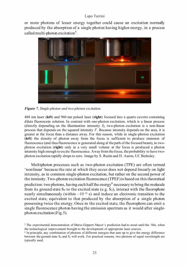
25
or more photons of lesser energy together could cause an excitation normally produced by the absorption of a single photon having higher energy, in a process called multi-photon excitation5.
Figure 7. Single-photon and two-photon excitation.
488 nm laser (left) and 960 nm pulsed laser (right) focused into a quartz cuvette containing dilute fluorescein solution. In contrast with one-photon excitation, which is a linear process (directly depending on the illumination intensity I), two-photon excitation is a non-linear process that depends on the squared intensity I2. Because intensity depends on the area, it is greater at the focus than a distance away. For this reason, while in single-photon excitation (left) the density of photon away from the focus is sufficient to produce emission of fluorescence (and thus fluorescence is generated along al the path of the focused beam), in two-photon excitation (right) only in a very small volume at the focus is produced a photon intensity high enough to excite fluorescence. Away from the focus, the probability to have two-photon excitation rapidly drops to zero. Image by S. Ruzin and H. Aaron, UC Berkeley.
Multiphoton processes such as two-photon excitation (TPE) are often termed ‘nonlinear’ because the rate at which they occur does not depend linearly on light intensity, as in common single-photon excitation, but rather on the second power of the intensity. Two-photon excitation fluorescence (TPEF) is based on this theoretical prediction: two photons, having each half the energy6 necessary to bring the molecule from its ground state S0 to the excited state (e.g. S2), interact with the fluorophore nearly simultaneously (within ~10-16 s) and induce an electronic transition to the excited state, equivalent to that produced by the absorption of a single photon possessing twice the energy. Once in the excited state, the fluorophore can emit a single fluorescence photon having the emission spectrum as it would after single-photon excitation (Fig.5).
5 The experimental demonstration of Maria Göppert-Mayer’s prediction had to await until the ’60s, when the technological improvement brought to the development of appropriate laser sources. 6 In principle, any combination of photons of different energies that sum up to give the energy difference between the ground state S0 and S2 will work. For practical reasons, two photons of equal wavelength are typically used.
24
Lapo Turrini
24
mirror image of S0 → S1 absorption as a result of the same transitions being involved in both absorption and emission, and similar vibrational energy levels of S0 and S1. Another general property of fluorescence is that the same fluorescence emission spectrum is typically observed regardless of the excitation wavelength (Fig.6). This is known as Kasha’s rule (Kasha, 1950) and result from the fact that, upon excitation into higher electronic and vibrational levels, the excess of energy is quickly dissipated in a non-radiative way, leaving the fluorophore in the lowest vibrational level of S1. Apart from some exceptions, due to internal conversion, fluorophores always emit from S1, and thus emission spectra are usually independent of excitation wavelength.
Figure 6. Fluorescence spectrum.
Example of excitation (blue) and emission (red) spectrum of a fluorophore. The emission spectrum is always (apart for some rare exceptions) shifted towards longer wavelengths with respect to the excitation spectrum (Stoke’s shift). The emission spectrum will have the same distribution regardless the excitation wavelength (Kasha’s rule). Due to the manifold vibrational levels present in each molecular electronic state, both excitation and emission spectra are not single bands (as happens in atomic spectra, for example) but have a broader distribution. The more vibrational levels a molecule has in its electronic states, the broader will result its fluorescence spectrum.
3.1 Two-photon excitation fluorescence
At the dawn of the development of quantum mechanics, Maria Göppert -Mayer (Göppert-Mayer, 1931) in her doctoral dissertation theorized an alternative mechanism through which fluorescence could be excited. She hypothesized that two
25
or more photons of lesser energy together could cause an excitation normally produced by the absorption of a single photon having higher energy, in a process called multi-photon excitation5.
Figure 7. Single-photon and two-photon excitation.
488 nm laser (left) and 960 nm pulsed laser (right) focused into a quartz cuvette containing dilute fluorescein solution. In contrast with one-photon excitation, which is a linear process (directly depending on the illumination intensity I), two-photon excitation is a non-linear process that depends on the squared intensity I2. Because intensity depends on the area, it is greater at the focus than a distance away. For this reason, while in single-photon excitation (left) the density of photon away from the focus is sufficient to produce emission of fluorescence (and thus fluorescence is generated along al the path of the focused beam), in two-photon excitation (right) only in a very small volume at the focus is produced a photon intensity high enough to excite fluorescence. Away from the focus, the probability to have two-photon excitation rapidly drops to zero. Image by S. Ruzin and H. Aaron, UC Berkeley.
Multiphoton processes such as two-photon excitation (TPE) are often termed ‘nonlinear’ because the rate at which they occur does not depend linearly on light intensity, as in common single-photon excitation, but rather on the second power of the intensity. Two-photon excitation fluorescence (TPEF) is based on this theoretical prediction: two photons, having each half the energy6 necessary to bring the molecule from its ground state S0 to the excited state (e.g. S2), interact with the fluorophore nearly simultaneously (within ~10-16 s) and induce an electronic transition to the excited state, equivalent to that produced by the absorption of a single photon possessing twice the energy. Once in the excited state, the fluorophore can emit a single fluorescence photon having the emission spectrum as it would after single-photon excitation (Fig.5).
5 The experimental demonstration of Maria Göppert-Mayer’s prediction had to await until the ’60s, when the technological improvement brought to the development of appropriate laser sources. 6 In principle, any combination of photons of different energies that sum up to give the energy difference between the ground state S0 and S2 will work. For practical reasons, two photons of equal wavelength are typically used.
25

Real-time whole-brain functional imaging of zebrafi sh neuronal activity
26
Since TPE is an extremely unlikely phenomenon, high intensity (the number of photons passing through a unit area per unit time, photons·cm-2·s-1) is required to produce TPEF. To attain high intensity, the excitation photons must be concentrated both spatially and temporally. High spatial photon density is obtained by focusing the laser beam to a diffraction-limited volume through a moderate/high numerical aperture (NA) objective. High temporal photon density is achieved using mode-locked pulsed lasers7 emitting photons intermittently in high-power bursts (instead of the most common continuous-wave ones). Consequently, only in the focal volume the spatio-temporal photon density is high enough to produce TPEF. Away from the focus, the TPE probability decrease rapidly so that no appreciable fluorescence is excited (Fig. 7).
7 The titanium:sapphire (Ti:Sa) laser generally adopted in two-photon fluorescence microscopy (TPFM) (Denk et al., 1990) generates picoseconds to hundreds of femtosecond pulses of high peak power, but at a low repetition rate (~100 MHz) thus keeping low the average power.
27
Chapter 4The Green Fluorescent Protein
Among all fluorophores, probably the most famous, and for sure the one that in biology research deserves a place of honour, is the green fluorescent protein (GFP). It was first discovered fortuitously in 1961 by Osamu Shimomura and colleagues (Shimomura O. et al., 1962) during the extraction and purification of the biolumines-
Figure 8. Aequorea victoria.A. victoria is a small (7-10 cm in diameter) marine jellyfish whose fame is due to the presence, along its umbrella rim-edge of light-emitting organs. In the dark, A. victoria’s luminescence is characteristically green owing to the emission of the green fluorescent protein. From (Shimomura, 2005).
26

26
Since TPE is an extremely unlikely phenomenon, high intensity (the number of photons passing through a unit area per unit time, photons·cm-2·s-1) is required to produce TPEF. To attain high intensity, the excitation photons must be concentrated both spatially and temporally. High spatial photon density is obtained by focusing the laser beam to a diffraction-limited volume through a moderate/high numerical aperture (NA) objective. High temporal photon density is achieved using mode-locked pulsed lasers7 emitting photons intermittently in high-power bursts (instead of the most common continuous-wave ones). Consequently, only in the focal volume the spatio-temporal photon density is high enough to produce TPEF. Away from the focus, the TPE probability decrease rapidly so that no appreciable fluorescence is excited (Fig. 7).
7 The titanium:sapphire (Ti:Sa) laser generally adopted in two-photon fluorescence microscopy (TPFM) (Denk et al., 1990) generates picoseconds to hundreds of femtosecond pulses of high peak power, but at a low repetition rate (~100 MHz) thus keeping low the average power.
27
Chapter 4The Green Fluorescent Protein
Among all fluorophores, probably the most famous, and for sure the one that in biology research deserves a place of honour, is the green fluorescent protein (GFP). It was first discovered fortuitously in 1961 by Osamu Shimomura and colleagues (Shimomura O. et al., 1962) during the extraction and purification of the biolumines-
Figure 8. Aequorea victoria.A. victoria is a small (7-10 cm in diameter) marine jellyfish whose fame is due to the presence, along its umbrella rim-edge of light-emitting organs. In the dark, A. victoria’s luminescence is characteristically green owing to the emission of the green fluorescent protein. From (Shimomura, 2005).
Lapo Turrini, Development of optical methods for real-time whole-brain functional imaging of zebrafi sh neuronal activity, © 2020 Author(s), content CC BY 4.0 International, metadata CC0 1.0 Universal, published by Firenze University Press (www.fupress.com), ISSN 2612-8020 (online), ISBN 978-88-5518-070-2 (PDF), DOI 10.36253/978-88-5518-070-2

Real-time whole-brain functional imaging of zebrafish neuronal activity
28
cent protein aequorin8 from the hydromedusan Aequorea victoria (Fig.8). GFP was isolated as a by-product of aequorin owing to the bright greenish colour it gave to the solution in which it was suspended9. The same group (Johnson F.H. et al., 1962) published then the emission spectrum of GFP, which peaked at 508 nm. They noted that the green bioluminescence of living Aequorea tissue also peaked near this wavelength, whereas the chemiluminescence of pure aequorin was blue and peaked near 470 nm, which was close to one of the excitation peaks of GFP. Therefore, Shimomura and colleagues hypothesized that GFP converted the blue emission of aequorin to the green one of the living jellyfish. Morin and Hastings in 1971 (Morin J.G. and Hastings J.W., 1971) first hypothesized the implication of a non-radiative Förster-type energy transfer from aequorin to GFP. The FRET mechanism was confirmed in 1974 by Morise and colleagues (Morise et al., 1974), who first purified and crystallized GFP.
Figure 9. GFP structure and fluorescence spectrum.
a. Crystal structure of GFP showing the typical 40 Å β-barrel, composed by 11 β strands, sheltering the fluorophore that consist of Ser65, Tyr66 and Gly67. From (Craggs, 2009). b. EGFP fluorescence spectrum has its excitation and emission peaks at 488 nm and 510 nm, respectively. With respect to wtGFP, the excitation peak in the UV range is absent owing to S65T mutation, which allows the fluorophore to remain in the deprotonated (anionic) state.
From a structural point of view (Fig.9), GFP is a 238 amino acids β-barrel consisting of eleven β-strands, threaded by an α-helix running up the axis of the barrel (27 kDa). The chromophore is attached to the α-helix and is hidden in the centre of the cylinder, which has been called a β-can. In 1979, Shimomura (Shimomura O., 1979) proteolysed denatured GFP, analysed the peptide that retained visible absorbance, and correctly proposed that the chromophore is 4-(p-hydroxybenzylidene)imidazolidin-5-one. The chromophore is formed, through a maturation process, by residues 65-66-67, which are Ser-Tyr-Gly in the native protein. After the protein has folded into its nearly native conformation, the imidazolinone is formed by nucleophilic attack of the amide of Gly67 on the carbonyl of Ser65, followed by dehydration. Finally, molecular oxygen dehydrogenates the α-β bond of
8 Aequorin is a protein that can bind calcium ions through three EF-hand domains. Upon Ca2+ binding, through an oxidative reaction, aequorin emits blue light (465 nm) (Shimomura O. and Johnson F.H., 1970;Inouye S. and Sasaki S., 2006). 9 Actually, the protein was first called “green protein” by Shimomura and colleagues; it was Hastings and Morin (Hastings J.W. and Morin J.G., 1969) in 1969 to use for the first time the term “green fluorescent protein”.
29
Tyr66, conjugating its aromatic group with the imidazolinone. Only at this stage, the chromophore does acquire visible absorbance and fluorescence. The peculiar position of the chromophore inside the β-barrel, protecting it from the environment, prevents it from quenching. Indeed, the β-barrel may have evolved to be porous during chromophore formation, thereby allowing the access of water and oxygen molecules, which seem to be fundamental for the correct chromophore maturation, and to be progressively more impermeable following chromophore formation (Li B. et al., 2012).
From a spectral point of view, GFP is characterized by two separate absorption peaks, a major one in the UV range at 395 nm and a minor one in the visible range at 475 nm. The amplitude of these absorption peaks changes according to pH level (Ward et al., 1982) (e.g. increasing pH increases the amplitude of the 475 nm excitation peak with a reduction of the 395 nm peak) and the excitation at 395 nm and at 475 nm gives two slightly different emission peaks, 508 and 503 nm respectively. This behaviour depends on the protonation state of the chromophore, in particular of the Tyr66. The 475 nm excitation peak arises from GFP molecules having deprotonated chromophores (anionic), whereas the 395 nm peak arises from GFPs containing protonated chromophores (neutral) (Heim et al., 1994;Cubitt et al., 1995). Protonated chromophores in the excited state are likely to deprotonate, because the phenol of the Tyr66 residue is prone to become much more acidic in its excited state. During most light absorption/emission cycles, the proton transfer does reverse. However, occasionally the proton does not return to the chromophore, so the neutral chromophore is photoisomerized to its anionic form. This behaviour accounts for the fact that upon intense UV illumination, the 395 nm absorption peak of the neutral form gradually decreases, and the 470-nm peak of the anionic chromophore increases (Cubitt et al., 1995;Chattoraj et al., 1996;Yokoe and Meyer, 1996).
An important breakthrough in the early history of GFP came with the isolation and cloning of the gene encoding GFP by Prasher and colleagues (Prasher et al., 1992) in 1992. Thanks to this great advancement, Chalfie and colleagues (Chalfie et al., 1994) in 1994 first showed that GFP could be heterologously expressed maintaining its fluorescent properties, and could, thus, be used as a marker for protein localization and expression in living organisms. They successfully expressed GFP in C. elegans under the control of a β-tubulin promoter active in touch receptor neurons. Its spatial and temporal expression in these specific neurons of the worm mimicked that of the endogenous β-tubulin gene, thus proving that GFP could be a faithful marker to study gene expression.
Once demonstrated the feasibility of using GFP as a versatile reporter of gene expression in vivo, great efforts were made to improve the wild-type GFP and to produce new spectral variants. Roger Y. Tsien is undoubtedly the scientist who gave the major contribution to the engineering of fluorescent proteins (FPs). Tsien, between 1994 and 1996, through random chromophore mutagenesis, produced a GFP variant 5-fold brighter than wtGFP characterized by a single excitation peak at 488 nm and improved folding at 37 °C, that after this was later named enhanced GFP (EGFP, S65T and F64L mutations) (Heim et al., 1995). He developed spectral GFP variants as well, such as the blue fluorescent protein (BFP, Y66H) and cyan fluorescent protein (CFP, Y66W) (Heim et al., 1994;Heim and Tsien, 1996). On the basis of GFP structural data
28
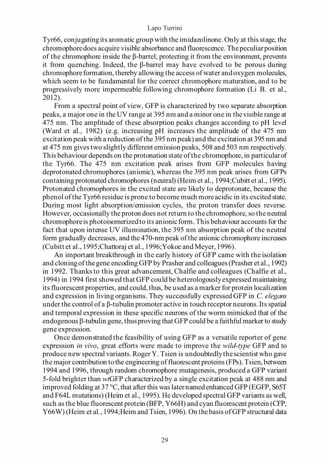
Lapo Turrini
28
cent protein aequorin8 from the hydromedusan Aequorea victoria (Fig.8). GFP was isolated as a by-product of aequorin owing to the bright greenish colour it gave to the solution in which it was suspended9. The same group (Johnson F.H. et al., 1962) published then the emission spectrum of GFP, which peaked at 508 nm. They noted that the green bioluminescence of living Aequorea tissue also peaked near this wavelength, whereas the chemiluminescence of pure aequorin was blue and peaked near 470 nm, which was close to one of the excitation peaks of GFP. Therefore, Shimomura and colleagues hypothesized that GFP converted the blue emission of aequorin to the green one of the living jellyfish. Morin and Hastings in 1971 (Morin J.G. and Hastings J.W., 1971) first hypothesized the implication of a non-radiative Förster-type energy transfer from aequorin to GFP. The FRET mechanism was confirmed in 1974 by Morise and colleagues (Morise et al., 1974), who first purified and crystallized GFP.
Figure 9. GFP structure and fluorescence spectrum.
a. Crystal structure of GFP showing the typical 40 Å β-barrel, composed by 11 β strands, sheltering the fluorophore that consist of Ser65, Tyr66 and Gly67. From (Craggs, 2009). b. EGFP fluorescence spectrum has its excitation and emission peaks at 488 nm and 510 nm, respectively. With respect to wtGFP, the excitation peak in the UV range is absent owing to S65T mutation, which allows the fluorophore to remain in the deprotonated (anionic) state.
From a structural point of view (Fig.9), GFP is a 238 amino acids β-barrel consisting of eleven β-strands, threaded by an α-helix running up the axis of the barrel (27 kDa). The chromophore is attached to the α-helix and is hidden in the centre of the cylinder, which has been called a β-can. In 1979, Shimomura (Shimomura O., 1979) proteolysed denatured GFP, analysed the peptide that retained visible absorbance, and correctly proposed that the chromophore is 4-(p-hydroxybenzylidene)imidazolidin-5-one. The chromophore is formed, through a maturation process, by residues 65-66-67, which are Ser-Tyr-Gly in the native protein. After the protein has folded into its nearly native conformation, the imidazolinone is formed by nucleophilic attack of the amide of Gly67 on the carbonyl of Ser65, followed by dehydration. Finally, molecular oxygen dehydrogenates the α-β bond of
8 Aequorin is a protein that can bind calcium ions through three EF-hand domains. Upon Ca2+ binding, through an oxidative reaction, aequorin emits blue light (465 nm) (Shimomura O. and Johnson F.H., 1970;Inouye S. and Sasaki S., 2006). 9 Actually, the protein was first called “green protein” by Shimomura and colleagues; it was Hastings and Morin (Hastings J.W. and Morin J.G., 1969) in 1969 to use for the first time the term “green fluorescent protein”.
29
Tyr66, conjugating its aromatic group with the imidazolinone. Only at this stage, the chromophore does acquire visible absorbance and fluorescence. The peculiar position of the chromophore inside the β-barrel, protecting it from the environment, prevents it from quenching. Indeed, the β-barrel may have evolved to be porous during chromophore formation, thereby allowing the access of water and oxygen molecules, which seem to be fundamental for the correct chromophore maturation, and to be progressively more impermeable following chromophore formation (Li B. et al., 2012).
From a spectral point of view, GFP is characterized by two separate absorption peaks, a major one in the UV range at 395 nm and a minor one in the visible range at 475 nm. The amplitude of these absorption peaks changes according to pH level (Ward et al., 1982) (e.g. increasing pH increases the amplitude of the 475 nm excitation peak with a reduction of the 395 nm peak) and the excitation at 395 nm and at 475 nm gives two slightly different emission peaks, 508 and 503 nm respectively. This behaviour depends on the protonation state of the chromophore, in particular of the Tyr66. The 475 nm excitation peak arises from GFP molecules having deprotonated chromophores (anionic), whereas the 395 nm peak arises from GFPs containing protonated chromophores (neutral) (Heim et al., 1994;Cubitt et al., 1995). Protonated chromophores in the excited state are likely to deprotonate, because the phenol of the Tyr66 residue is prone to become much more acidic in its excited state. During most light absorption/emission cycles, the proton transfer does reverse. However, occasionally the proton does not return to the chromophore, so the neutral chromophore is photoisomerized to its anionic form. This behaviour accounts for the fact that upon intense UV illumination, the 395 nm absorption peak of the neutral form gradually decreases, and the 470-nm peak of the anionic chromophore increases (Cubitt et al., 1995;Chattoraj et al., 1996;Yokoe and Meyer, 1996).
An important breakthrough in the early history of GFP came with the isolation and cloning of the gene encoding GFP by Prasher and colleagues (Prasher et al., 1992) in 1992. Thanks to this great advancement, Chalfie and colleagues (Chalfie et al., 1994) in 1994 first showed that GFP could be heterologously expressed maintaining its fluorescent properties, and could, thus, be used as a marker for protein localization and expression in living organisms. They successfully expressed GFP in C. elegans under the control of a β-tubulin promoter active in touch receptor neurons. Its spatial and temporal expression in these specific neurons of the worm mimicked that of the endogenous β-tubulin gene, thus proving that GFP could be a faithful marker to study gene expression.
Once demonstrated the feasibility of using GFP as a versatile reporter of gene expression in vivo, great efforts were made to improve the wild-type GFP and to produce new spectral variants. Roger Y. Tsien is undoubtedly the scientist who gave the major contribution to the engineering of fluorescent proteins (FPs). Tsien, between 1994 and 1996, through random chromophore mutagenesis, produced a GFP variant 5-fold brighter than wtGFP characterized by a single excitation peak at 488 nm and improved folding at 37 °C, that after this was later named enhanced GFP (EGFP, S65T and F64L mutations) (Heim et al., 1995). He developed spectral GFP variants as well, such as the blue fluorescent protein (BFP, Y66H) and cyan fluorescent protein (CFP, Y66W) (Heim et al., 1994;Heim and Tsien, 1996). On the basis of GFP structural data
29

Real-time whole-brain functional imaging of zebrafish neuronal activity
30
instead, he designed and generated the yellow fluorescent protein (YFP, T203Y) (Ormo et al., 1996).
In 2008, the Nobel Prize in Chemistry was awarded jointly to Osamu Shimomura, Martin Chalfie and Roger Y. Tsien “for the discovery and development of the green fluorescent protein, GFP”.
31
Chapter 5 Genetically encoded Ca2+ indicators
During the course of cellular evolution, calcium ion (Ca2+) has been selected as a universal carrier of signals. Noting its extensive distribution and functioning as a control ion in cells, common to a huge range of eukaryote cell types, from animal, plant, to fungal, which diverged billions of years ago, it is clear how early in the evolutionary history this ion earned its fundamental role in cell life (Williams, 1999).
The first observation of the signalling role of Ca2+ is due to Sydney Ringer while performing experiments on the contraction of isolated rat hearts10 (Ringer, 1883) in 1883. Ever since, this topic attracted great attention from the scientific community and many more evidence of Ca2+ implication in the most diverse aspects of cell metabolism were brought to light. Actually, the variety of processes that are controlled by Ca2+ begins with the origin of cell life at fertilization, and ends with apoptosis, the process of programmed death that terminates life once cells have reached the end of their vital cycle. Between these two events, Ca2+ regulates processes that may be shared by all cells, e.g. differentiation, gene transcription, control of phosphorylation grade, cytoskeletal reorganization, and cell motility. Other processes may be otherwise cell-type specific, e.g. contraction/relaxation of skeletal muscles and heart, secretion of insulin in pancreatic β-cell and neurotransmitters in pre-synaptic nerve cells.
In neurons during an action potential, the changes in permeability, caused by the opening of gated ion channels, modify the net charge separation across the membrane and thus produce an electric signal, but typically do not result in appreciable changes in the bulk intracellular concentrations of most ion species (Hodgkin and Huxley, 1952). Ca2+ is a notable exception to this rule. The concentration of free Ca2+ in the cytoplasm of a resting cell is kept extremely low, about 10-4 mM, several orders of magnitude below the external Ca2+ concentration, which is approximately 2 mM. Due to this steep gradient, the intracellular Ca2+ concentration may increase many fold above the resting value as a result of the influx of calcium through membrane voltage-gated Ca2+ channels (Baker et al., 1971). This inward ICa helps depolarize the cell and at the same time enhances the probability that calcium-activated, voltage-sensitive K+ channels will open, thus triggering cell repolarization through outward potassium
10 Ringer came almost by chance to the discovery that Ca2+ carried the signal that initiated heart contraction. As he admitted, in early experiments, he had suspended the isolated hearts in a saline solution prepared using London tap water and the hearts contracted beautifully. When he proceeded to replace tap water with distilled water, he made a surprising finding: the beating of hearts became progressively weaker until stopping. To maintain contraction, he found it necessary to add Ca2+ salts to the suspension medium.
30

30
instead, he designed and generated the yellow fluorescent protein (YFP, T203Y) (Ormo et al., 1996).
In 2008, the Nobel Prize in Chemistry was awarded jointly to Osamu Shimomura, Martin Chalfie and Roger Y. Tsien “for the discovery and development of the green fluorescent protein, GFP”.
31
Chapter 5 Genetically encoded Ca2+ indicators
During the course of cellular evolution, calcium ion (Ca2+) has been selected as a universal carrier of signals. Noting its extensive distribution and functioning as a control ion in cells, common to a huge range of eukaryote cell types, from animal, plant, to fungal, which diverged billions of years ago, it is clear how early in the evolutionary history this ion earned its fundamental role in cell life (Williams, 1999).
The first observation of the signalling role of Ca2+ is due to Sydney Ringer while performing experiments on the contraction of isolated rat hearts10 (Ringer, 1883) in 1883. Ever since, this topic attracted great attention from the scientific community and many more evidence of Ca2+ implication in the most diverse aspects of cell metabolism were brought to light. Actually, the variety of processes that are controlled by Ca2+ begins with the origin of cell life at fertilization, and ends with apoptosis, the process of programmed death that terminates life once cells have reached the end of their vital cycle. Between these two events, Ca2+ regulates processes that may be shared by all cells, e.g. differentiation, gene transcription, control of phosphorylation grade, cytoskeletal reorganization, and cell motility. Other processes may be otherwise cell-type specific, e.g. contraction/relaxation of skeletal muscles and heart, secretion of insulin in pancreatic β-cell and neurotransmitters in pre-synaptic nerve cells.
In neurons during an action potential, the changes in permeability, caused by the opening of gated ion channels, modify the net charge separation across the membrane and thus produce an electric signal, but typically do not result in appreciable changes in the bulk intracellular concentrations of most ion species (Hodgkin and Huxley, 1952). Ca2+ is a notable exception to this rule. The concentration of free Ca2+ in the cytoplasm of a resting cell is kept extremely low, about 10-4 mM, several orders of magnitude below the external Ca2+ concentration, which is approximately 2 mM. Due to this steep gradient, the intracellular Ca2+ concentration may increase many fold above the resting value as a result of the influx of calcium through membrane voltage-gated Ca2+ channels (Baker et al., 1971). This inward ICa helps depolarize the cell and at the same time enhances the probability that calcium-activated, voltage-sensitive K+ channels will open, thus triggering cell repolarization through outward potassium
10 Ringer came almost by chance to the discovery that Ca2+ carried the signal that initiated heart contraction. As he admitted, in early experiments, he had suspended the isolated hearts in a saline solution prepared using London tap water and the hearts contracted beautifully. When he proceeded to replace tap water with distilled water, he made a surprising finding: the beating of hearts became progressively weaker until stopping. To maintain contraction, he found it necessary to add Ca2+ salts to the suspension medium. Lapo Turrini, Development of optical methods for real-time whole-brain functional imaging of zebrafish neuronal activity, © 2020 Author(s), content CC BY 4.0 International, metadata CC0 1.0 Universal, published by Firenze University Press (www.fupress.com), ISSN 2612-8020 (online), ISBN 978-88-5518-070-2 (PDF), DOI 10.36253/978-88-5518-070-2

Real-time whole-brain functional imaging of zebrafish neuronal activity
32
current. Right after the end of an action potential, during the repolarization phase, the cytoplasmic Ca2+ concentration is brought back to its basal levels through an array of calcium transporters. These ion pumps belong to the superfamily of P-type ATPases and either extruding calcium outside the cell (plasma membrane Ca2+ ATPase, PMCAs) or segregating it in intracellular compartments such as endoplasmic reticulum (sarco/endoplasmic reticulum Ca2+ ATPase, SERCAs) and Golgi vesicles system (secretory pathway Ca2+ ATPase, SPCAs), they contribute to diminish free calcium inside the neuron (Pedersen and Carofoli, 1987). Additionally, mitochondria can act as calcium buffers by taking Ca2+ up through the calcium uniporter (Duchen, 1999).
Hence, in a neuron, the short-term fluctuation of intracellular Ca2+ concentration reflects its activation state and thus measuring this fluctuation one could have an indirect recording of neuronal activity.
Owing to the crucial role of Ca2+ and its homeostasis as universal signalling ion, profuse were the efforts to develop methods that would give the possibility to measure intracellular Ca2+ dynamics. In particular, research focused on the development of fluorescent molecules having the ability to bind Ca2+ and to modulate their emission depending on Ca2+ concentration. Reliable methods to measure cytosolic Ca2+ concentration appeared in the late 1960s, when Ridgway and Ashley (Ridgway and Ashley, 1967) first exploited the Ca2+-dependent bioluminescence of aequorin to observe transient Ca2+ signals in single isolated muscle fibres of barnacle. While aequorin provided important early insights into the calcium-dependent regulation of neuronal processes (Hallett and Carbone, 1972;Stinnakre and Tauc, 1973;Llinas and Nicholson, 1975), its implementation and use was often inconvenient. In fact, the use of the purified protein, as in Ridgway and Ashley experiments, required its injection inside the desired tissue or cells, while when pursuing recombinant expression of aequorin it was necessary to administer coelenterazine as a cofactor of the translated apoenzyme in order to have the functional protein, limiting its application to cell cultures. A true breakthrough came a few years later, when Roger Y. Tsien (Tsien, 1980) rationally designed and developed a new generation of synthetic fluorescent polycarboxilate dyes derived from the hybridization of the highly calcium-sensitive chelator EGTA with a fluorescent chromophore. The first generation of fluorescent calcium indicators included BAPTA and its derivative Quin-2, which, excited by UV light, was the first dye used in biological experiments (Pozzan et al., 1982;Tsien et al., 1982). However, these dyes required complex loading procedures, which often ended up damaging the sample. Critical to the widespread popularity of the polycarboxilate Ca2+ indicators was the synthesis of their acetoxymethyl (AM) esters which, being membrane permeable, allow for non-disruptive loading and efficient trapping of the dyes in intact cells once the ester groups are hydrolysed (Tsien, 1981). In 1985, Tsien and colleagues (Grynkiewicz et al., 1985) introduced a second generation of improved indicators (e.g. Fura-2, Indo-1, etc) with stronger fluorescence emission upon Ca2+ binding, weaker affinity for Ca2+ and higher specificity (i.e. better selectivity against other ions). Fura-2 allowed the same group (Williams et al., 1985) to perform unprecedented spatiotemporal measurements of Ca2+ gradients in subcellular compartments of single smooth muscle cells, revealing the differential regulation of Ca2+ concentration in the cytoplasm, nucleus and sarcoplasmic
33
reticulum. Despite the substantial advancement, one disadvantage of the Fura-2 family of dyes, which limited their range of potential application, in particular in in vivo experiments, was that they required excitation in the UV. For this reason, Tsien and colleagues further developed their indicators, producing a novel class of Ca2+ reporters (Rhod-2, Fluo-2, Fluo-3, etc.) having visible-wavelength excitation (Minta et al., 1989). These Ca2+ indicators and their further improved versions (e.g. Fluo-4 (Gee et al., 2000), Oregon Green BAPTA-1) have achieved widespread use in neuroscience research (Ohki et al., 2005;Sullivan et al., 2005;Greenberg et al., 2008;Li et al., 2008;Sumbre et al., 2008;Dombeck et al., 2010), thanks to their brightness, photostability and very large Ca2+-dependent fluorescent changes.
The major limitation of Ca2+-sensitive dyes arises from their impossibility to selectively stain specific cellular populations or different subcellular compartments, considerably reducing the range of in vivo applications. The demonstration by Chalfie and colleagues (Chalfie et al., 1994) in 1994, that GFP could be effectively expressed in multicellular organisms under the control of a specific gene promoter, without the need for exogenous substrates and cofactors coming from the jellyfish, paved the way for the development of a new class of Ca2+ reporters with genetic tagging. In 1997, again the laboratory of Roger Y. Tsien (Miyawaki et al., 1997), brought to light the first Ca2+ sensor based on GFP: that was how genetically encoded calcium indicators (GECIs) were born. Cameleon, as it was called, was based on a simple and yet brilliant design. A CFP molecule was fused to the N-terminus of calmodulin (CaM), an eukaryotic protein with four EF-hand Ca2+-binding domains, and a YFP to the C-terminus of M13, the CaM-binding peptide from skeletal muscle myosin light chain kinase. The CFP-CaM and the M13-YFP were linked by two glycines. Reversible binding of Ca2+ to the CaM caused it to bind the M13 (Porumb et al., 1996), bringing CFP and YFP close enough to produce FRET. Hence, an increase in intracellular Ca2+ concentration resulted in increased YFP emission upon CFP excitation. The innovative rational design of Cameleon-1 and Cameleon-2 (a variant with different FRET partners, BFP-GFP), which exploited the physiological interaction occurring between CaM and M13 peptide, represents the functional unit of almost all the GECIs that would have been later developed. In 1999, again Tsien group (Baird et al., 1999), discovered that the β-can surrounding the chromophore of GFP could be circularly permuted (cp), opening the way to the development of single-FP based indicators. The circular permutation consists in the insertion of a peptide linker between N- and C-terminus of the protein and the creation of a new N- and C-terminus pair, elsewhere in the sequence. The discovery lead to the development of Camgaroo, the first single-fluorophore GECI, a circularly permuted enhanced YFP (cpEYFP) bringing a CaM domain between positions 144 and 145, near the chromophore. The conformational change occurring in the β-barrel, upon Ca2+ binding, was responsible for the increase in emitted fluorescence.
In 2001, Pericam (Nagai et al., 2001) and GCaMP (Nakai et al., 2001) were separately developed, yet on a common design: both had a circularly permuted FP – cpEYFP the first and cpGFP the second – carrying the M13 peptide fused to the C-terminus and the CaM domain to the N-terminus. Both indicators shared the same working mechanism. The fusion of CaM domain and M13 peptide to the cpFP, introduces a distortion in the β-can structure that induces the quenching of
32

Lapo Turrini
32
current. Right after the end of an action potential, during the repolarization phase, the cytoplasmic Ca2+ concentration is brought back to its basal levels through an array of calcium transporters. These ion pumps belong to the superfamily of P-type ATPases and either extruding calcium outside the cell (plasma membrane Ca2+ ATPase, PMCAs) or segregating it in intracellular compartments such as endoplasmic reticulum (sarco/endoplasmic reticulum Ca2+ ATPase, SERCAs) and Golgi vesicles system (secretory pathway Ca2+ ATPase, SPCAs), they contribute to diminish free calcium inside the neuron (Pedersen and Carofoli, 1987). Additionally, mitochondria can act as calcium buffers by taking Ca2+ up through the calcium uniporter (Duchen, 1999).
Hence, in a neuron, the short-term fluctuation of intracellular Ca2+ concentration reflects its activation state and thus measuring this fluctuation one could have an indirect recording of neuronal activity.
Owing to the crucial role of Ca2+ and its homeostasis as universal signalling ion, profuse were the efforts to develop methods that would give the possibility to measure intracellular Ca2+ dynamics. In particular, research focused on the development of fluorescent molecules having the ability to bind Ca2+ and to modulate their emission depending on Ca2+ concentration. Reliable methods to measure cytosolic Ca2+ concentration appeared in the late 1960s, when Ridgway and Ashley (Ridgway and Ashley, 1967) first exploited the Ca2+-dependent bioluminescence of aequorin to observe transient Ca2+ signals in single isolated muscle fibres of barnacle. While aequorin provided important early insights into the calcium-dependent regulation of neuronal processes (Hallett and Carbone, 1972;Stinnakre and Tauc, 1973;Llinas and Nicholson, 1975), its implementation and use was often inconvenient. In fact, the use of the purified protein, as in Ridgway and Ashley experiments, required its injection inside the desired tissue or cells, while when pursuing recombinant expression of aequorin it was necessary to administer coelenterazine as a cofactor of the translated apoenzyme in order to have the functional protein, limiting its application to cell cultures. A true breakthrough came a few years later, when Roger Y. Tsien (Tsien, 1980) rationally designed and developed a new generation of synthetic fluorescent polycarboxilate dyes derived from the hybridization of the highly calcium-sensitive chelator EGTA with a fluorescent chromophore. The first generation of fluorescent calcium indicators included BAPTA and its derivative Quin-2, which, excited by UV light, was the first dye used in biological experiments (Pozzan et al., 1982;Tsien et al., 1982). However, these dyes required complex loading procedures, which often ended up damaging the sample. Critical to the widespread popularity of the polycarboxilate Ca2+ indicators was the synthesis of their acetoxymethyl (AM) esters which, being membrane permeable, allow for non-disruptive loading and efficient trapping of the dyes in intact cells once the ester groups are hydrolysed (Tsien, 1981). In 1985, Tsien and colleagues (Grynkiewicz et al., 1985) introduced a second generation of improved indicators (e.g. Fura-2, Indo-1, etc) with stronger fluorescence emission upon Ca2+ binding, weaker affinity for Ca2+ and higher specificity (i.e. better selectivity against other ions). Fura-2 allowed the same group (Williams et al., 1985) to perform unprecedented spatiotemporal measurements of Ca2+ gradients in subcellular compartments of single smooth muscle cells, revealing the differential regulation of Ca2+ concentration in the cytoplasm, nucleus and sarcoplasmic
33
reticulum. Despite the substantial advancement, one disadvantage of the Fura-2 family of dyes, which limited their range of potential application, in particular in in vivo experiments, was that they required excitation in the UV. For this reason, Tsien and colleagues further developed their indicators, producing a novel class of Ca2+ reporters (Rhod-2, Fluo-2, Fluo-3, etc.) having visible-wavelength excitation (Minta et al., 1989). These Ca2+ indicators and their further improved versions (e.g. Fluo-4 (Gee et al., 2000), Oregon Green BAPTA-1) have achieved widespread use in neuroscience research (Ohki et al., 2005;Sullivan et al., 2005;Greenberg et al., 2008;Li et al., 2008;Sumbre et al., 2008;Dombeck et al., 2010), thanks to their brightness, photostability and very large Ca2+-dependent fluorescent changes.
The major limitation of Ca2+-sensitive dyes arises from their impossibility to selectively stain specific cellular populations or different subcellular compartments, considerably reducing the range of in vivo applications. The demonstration by Chalfie and colleagues (Chalfie et al., 1994) in 1994, that GFP could be effectively expressed in multicellular organisms under the control of a specific gene promoter, without the need for exogenous substrates and cofactors coming from the jellyfish, paved the way for the development of a new class of Ca2+ reporters with genetic tagging. In 1997, again the laboratory of Roger Y. Tsien (Miyawaki et al., 1997), brought to light the first Ca2+ sensor based on GFP: that was how genetically encoded calcium indicators (GECIs) were born. Cameleon, as it was called, was based on a simple and yet brilliant design. A CFP molecule was fused to the N-terminus of calmodulin (CaM), an eukaryotic protein with four EF-hand Ca2+-binding domains, and a YFP to the C-terminus of M13, the CaM-binding peptide from skeletal muscle myosin light chain kinase. The CFP-CaM and the M13-YFP were linked by two glycines. Reversible binding of Ca2+ to the CaM caused it to bind the M13 (Porumb et al., 1996), bringing CFP and YFP close enough to produce FRET. Hence, an increase in intracellular Ca2+ concentration resulted in increased YFP emission upon CFP excitation. The innovative rational design of Cameleon-1 and Cameleon-2 (a variant with different FRET partners, BFP-GFP), which exploited the physiological interaction occurring between CaM and M13 peptide, represents the functional unit of almost all the GECIs that would have been later developed. In 1999, again Tsien group (Baird et al., 1999), discovered that the β-can surrounding the chromophore of GFP could be circularly permuted (cp), opening the way to the development of single-FP based indicators. The circular permutation consists in the insertion of a peptide linker between N- and C-terminus of the protein and the creation of a new N- and C-terminus pair, elsewhere in the sequence. The discovery lead to the development of Camgaroo, the first single-fluorophore GECI, a circularly permuted enhanced YFP (cpEYFP) bringing a CaM domain between positions 144 and 145, near the chromophore. The conformational change occurring in the β-barrel, upon Ca2+ binding, was responsible for the increase in emitted fluorescence.
In 2001, Pericam (Nagai et al., 2001) and GCaMP (Nakai et al., 2001) were separately developed, yet on a common design: both had a circularly permuted FP – cpEYFP the first and cpGFP the second – carrying the M13 peptide fused to the C-terminus and the CaM domain to the N-terminus. Both indicators shared the same working mechanism. The fusion of CaM domain and M13 peptide to the cpFP, introduces a distortion in the β-can structure that induces the quenching of
33

Real-time whole-brain functional imaging of zebrafish neuronal activity
34
chromophore fluorescence. Upon Ca2+ binding, the conformational change occurring in the β-can, because of M13/CaM interaction, restores the original shape of the barrel with an increase in emitted fluorescence. While Pericam development was abandoned, GCaMP (Fig.10) scaffold has been iteratively optimized in multiple rounds of structure-guided design, giving birth to the most widely used family of protein calcium sensors.
Figure 10. GCaMP structure and kinetic features.
Crystal structure of GCaMP showing the three domains of which is made: circularly permuted GFP (cpGFP), calmodulin (CaM), and myosin light chain kinase M13 peptide. With low intracellular Ca2+ concentration, upon blue light (488 nm) excitation, GCaMP emits dim baseline fluorescence. Increasing intracellular Ca2+ concentration, the binding of Ca2+ ions to the CaM domain induce a conformational change that restores the fluorophore emission properties, giving rise to bright fluorescence. The process is reversible. Table. Biophysical features of the last generations of GCaMP sensor.
The founder GCaMP had very weak fluorescence compared to GFP itself, when expressed at physiological temperatures. This issue was addressed by introducing two mutations (V163A and S175G) known to improve the temperature-dependent maturation of GFP, to give the variant called GCaMP1.6 (Ohkura et al., 2005), which had about 40-fold increased brightness. However, these modifications did not lead to adequate maturation above 30°C. Thus, the GCaMP construct was subjected to random mutagenesis. The clones showing brightest fluorescence at 37°C were selected and the corresponding mutations identified (D180Y and V93I) (Tallini et al., 2006). GCaMP2, as it was called, was 200 times brighter than GCaMP at 37°C. Then, attention was focused on improving the sensitivity of the indicator, to detect smaller calcium changes. The determination of GCaMP2 crystal structure in the Ca2+-bound
35
and Ca2+-free states (Wang et al., 2008;Akerboom et al., 2009), allowed the systematic mutagenesis of the CaM EF-hand and of the M13/CaM interaction domains, giving rise to GCaMP3 (Tian et al., 2009). This novel indicator showed an increased dynamic range, due to a 2-fold decrease in calcium-free fluorescence and 1.5-fold increase in calcium-saturated fluorescence with respect to GCaMP2. Targeted mutagenesis of the linkers connecting the cpGFP to CaM and the M13 peptide led then to GCaMP5 (Akerboom et al., 2012).
5.1 GCaMP6s
In 2013 what is, to date, the most sensitive protein calcium sensor was developed: GCaMP6 (Chen et al., 2013). Mutagenesis was directed towards the interface between cpGFP and CaM, M13 and CaM, and inside CaM domain. Due to the fast calcium dynamics and the low peak calcium accumulations typical of neurons (Sabatini et al., 2002), Chen et al. screened GCaMP6 variants produced by mutagenesis, in neurons. Based on the screening results, they isolated three ultrasensitive GCaMP6 variants (6s, 6m and 6f, for slow, medium and fast, respectively) characterized by different kinetics. Compared to GCaMP5, GCaMP6 have similar baseline brightness, with a 1.5-fold increase in dynamic range (Fig. 10, Table). For small numbers of action potential, the most sensitive sensor, GCaMP6s, produced sevenfold larger signals. Calcium-saturated GCaMP6s is 27% brighter than EGFP (Chen et al., 2013).
Due to the extremely rapid processes at the basis of neuronal communication (the duration of an action potential is typically in the order of 2 ms), even this last generation of Ca2+ sensors is far from having a kinetic fast enough to resolve single action potentials. In fact, even considering the fastest Ca2+-indicator currently available, GCaMP6f (Fig.10, Table), despite its potential sensitivity to detect a single AP, its overall rise and decay time approaches 200 ms, a time sufficient for tens of APs to happen. Indeed, the fluorescence dynamics recorded in in-vivo experiments is typically the result of tens, if not hundreds, of APs. Given the slow kinetic of the albeit fast GCaMP6 sensors, with respect to the electrical communication between neurons, a Ca2+ fluorescence time trace can be considered as the result of a powerful low-pass filter on the actual sequence of neuronal APs. Despite the direct relation between intracellular Ca2+ concentration and fluorescence emission characteristic of calcium sensors, these single FP based indicators (in contrast with FRET-based ones) do not allow an absolute quantification of Ca2+ concentration, and ultimately, thus, do not allow to perform inference about the number of action potentials underlying a fluorescence curve.
Present genetically encoded voltage indicators (GEVIs), have fast enough kinetics to reveal single action potentials; however, at the current stage of development, they do not have a sufficient signal-to-noise ratio (SNR) to be useful in-vivo beyond a very sparse neuronal labelling. Therefore, GCaMP6 indicators family represents, to date, the most useful optical tool to perform measurements of neuronal activity with pan-neuronal labelling. Coupled with zebrafish larvae as an animal model (see Zebrafish in neurosciences), GCaMP6 represents the best and most reliable neuronal activity indicator available, to perform whole brain recording with up to single cell resolution.
34

Lapo Turrini
34
chromophore fluorescence. Upon Ca2+ binding, the conformational change occurring in the β-can, because of M13/CaM interaction, restores the original shape of the barrel with an increase in emitted fluorescence. While Pericam development was abandoned, GCaMP (Fig.10) scaffold has been iteratively optimized in multiple rounds of structure-guided design, giving birth to the most widely used family of protein calcium sensors.
Figure 10. GCaMP structure and kinetic features.
Crystal structure of GCaMP showing the three domains of which is made: circularly permuted GFP (cpGFP), calmodulin (CaM), and myosin light chain kinase M13 peptide. With low intracellular Ca2+ concentration, upon blue light (488 nm) excitation, GCaMP emits dim baseline fluorescence. Increasing intracellular Ca2+ concentration, the binding of Ca2+ ions to the CaM domain induce a conformational change that restores the fluorophore emission properties, giving rise to bright fluorescence. The process is reversible. Table. Biophysical features of the last generations of GCaMP sensor.
The founder GCaMP had very weak fluorescence compared to GFP itself, when expressed at physiological temperatures. This issue was addressed by introducing two mutations (V163A and S175G) known to improve the temperature-dependent maturation of GFP, to give the variant called GCaMP1.6 (Ohkura et al., 2005), which had about 40-fold increased brightness. However, these modifications did not lead to adequate maturation above 30°C. Thus, the GCaMP construct was subjected to random mutagenesis. The clones showing brightest fluorescence at 37°C were selected and the corresponding mutations identified (D180Y and V93I) (Tallini et al., 2006). GCaMP2, as it was called, was 200 times brighter than GCaMP at 37°C. Then, attention was focused on improving the sensitivity of the indicator, to detect smaller calcium changes. The determination of GCaMP2 crystal structure in the Ca2+-bound
35
and Ca2+-free states (Wang et al., 2008;Akerboom et al., 2009), allowed the systematic mutagenesis of the CaM EF-hand and of the M13/CaM interaction domains, giving rise to GCaMP3 (Tian et al., 2009). This novel indicator showed an increased dynamic range, due to a 2-fold decrease in calcium-free fluorescence and 1.5-fold increase in calcium-saturated fluorescence with respect to GCaMP2. Targeted mutagenesis of the linkers connecting the cpGFP to CaM and the M13 peptide led then to GCaMP5 (Akerboom et al., 2012).
5.1 GCaMP6s
In 2013 what is, to date, the most sensitive protein calcium sensor was developed: GCaMP6 (Chen et al., 2013). Mutagenesis was directed towards the interface between cpGFP and CaM, M13 and CaM, and inside CaM domain. Due to the fast calcium dynamics and the low peak calcium accumulations typical of neurons (Sabatini et al., 2002), Chen et al. screened GCaMP6 variants produced by mutagenesis, in neurons. Based on the screening results, they isolated three ultrasensitive GCaMP6 variants (6s, 6m and 6f, for slow, medium and fast, respectively) characterized by different kinetics. Compared to GCaMP5, GCaMP6 have similar baseline brightness, with a 1.5-fold increase in dynamic range (Fig. 10, Table). For small numbers of action potential, the most sensitive sensor, GCaMP6s, produced sevenfold larger signals. Calcium-saturated GCaMP6s is 27% brighter than EGFP (Chen et al., 2013).
Due to the extremely rapid processes at the basis of neuronal communication (the duration of an action potential is typically in the order of 2 ms), even this last generation of Ca2+ sensors is far from having a kinetic fast enough to resolve single action potentials. In fact, even considering the fastest Ca2+-indicator currently available, GCaMP6f (Fig.10, Table), despite its potential sensitivity to detect a single AP, its overall rise and decay time approaches 200 ms, a time sufficient for tens of APs to happen. Indeed, the fluorescence dynamics recorded in in-vivo experiments is typically the result of tens, if not hundreds, of APs. Given the slow kinetic of the albeit fast GCaMP6 sensors, with respect to the electrical communication between neurons, a Ca2+ fluorescence time trace can be considered as the result of a powerful low-pass filter on the actual sequence of neuronal APs. Despite the direct relation between intracellular Ca2+ concentration and fluorescence emission characteristic of calcium sensors, these single FP based indicators (in contrast with FRET-based ones) do not allow an absolute quantification of Ca2+ concentration, and ultimately, thus, do not allow to perform inference about the number of action potentials underlying a fluorescence curve.
Present genetically encoded voltage indicators (GEVIs), have fast enough kinetics to reveal single action potentials; however, at the current stage of development, they do not have a sufficient signal-to-noise ratio (SNR) to be useful in-vivo beyond a very sparse neuronal labelling. Therefore, GCaMP6 indicators family represents, to date, the most useful optical tool to perform measurements of neuronal activity with pan-neuronal labelling. Coupled with zebrafish larvae as an animal model (see Zebrafish in neurosciences), GCaMP6 represents the best and most reliable neuronal activity indicator available, to perform whole brain recording with up to single cell resolution.
35

37
Chapter 6 Fluorescence microscopy
Ever since the first cytological and histological observations in the XIX century, the need emerged for methods aiming to enhance the contrast, in the sample, between structures of interest and not (background). In this direction went the development of staining procedures such as the black reaction by Camillo Golgi (Golgi, 1885) (see Fig.2), haematoxylin and eosin (Paul Mayer, 1896), and Giemsa stain (Gustav Giemsa, 1904). All of them are absorption techniques in which structures of interest are stained with agents that absorb light. The limit of these techniques lies in the fact that, for small objects, the amount of light absorbed becomes only infinitesimally different from the background. During the course of the XX century, owing to the growing theoretical knowledge around fluorescence phenomenon, several staining methods based on fluorescent molecules were developed. In fact, fluorescent labelling in the absence of autofluorescence allows for a dramatic increase in contrast of the structures of interest. Furthermore, owing to the possibility to genetically target the expression of fluorescent tags (GFP and its derivatives), the use of fluorescence in biology research has considerably increased over the past decades.
The basic but not trivial task of a fluorescence microscope is to irradiate the specimen with a desired and specific band of wavelengths, and then to separate the much weaker emitted fluorescence from the excitation light. The separation between the two (excitation and emission wavelength are different due to the Stoke’s shift phenomenon, see Fluorescence theory) is achieved using a fluorescence (or emission) filter. These filters have different transmittance (i.e. fraction of incident electromagnetic power that is transmitted) depending on light wavelength. According to the excitation and emission properties of the fluorophore in use, the right emission filter is the one that selectively blocks the excitation wavelength and is transparent to the fluorescence wavelength, so that only the last one can reach the detector. Fluorescence filters are typically band-pass filters, having high transmittance in the range of the fluorophore emission peak and almost zero transmittance outside the range, or long-pass filter, blocking shorter wavelengths and transmitting longer ones. Initially, fluorescence microscopes adopted a transmission (diascopic) configuration, in which the exciting light coming through the condenser is directed on the sample, and the emitted fluorescence is collected by the objective. However, the most widespread approach in modern fluorescence microscopes is epi-illumination. In this configuration, the microscope objective serves to both image and magnify the sample and to condense excitation light on it. The advantage of this approach over transmission is that, although the excitation of fluorophores is equivalent in both epi-
36

37
Chapter 6 Fluorescence microscopy
Ever since the first cytological and histological observations in the XIX century, the need emerged for methods aiming to enhance the contrast, in the sample, between structures of interest and not (background). In this direction went the development of staining procedures such as the black reaction by Camillo Golgi (Golgi, 1885) (see Fig.2), haematoxylin and eosin (Paul Mayer, 1896), and Giemsa stain (Gustav Giemsa, 1904). All of them are absorption techniques in which structures of interest are stained with agents that absorb light. The limit of these techniques lies in the fact that, for small objects, the amount of light absorbed becomes only infinitesimally different from the background. During the course of the XX century, owing to the growing theoretical knowledge around fluorescence phenomenon, several staining methods based on fluorescent molecules were developed. In fact, fluorescent labelling in the absence of autofluorescence allows for a dramatic increase in contrast of the structures of interest. Furthermore, owing to the possibility to genetically target the expression of fluorescent tags (GFP and its derivatives), the use of fluorescence in biology research has considerably increased over the past decades.
The basic but not trivial task of a fluorescence microscope is to irradiate the specimen with a desired and specific band of wavelengths, and then to separate the much weaker emitted fluorescence from the excitation light. The separation between the two (excitation and emission wavelength are different due to the Stoke’s shift phenomenon, see Fluorescence theory) is achieved using a fluorescence (or emission) filter. These filters have different transmittance (i.e. fraction of incident electromagnetic power that is transmitted) depending on light wavelength. According to the excitation and emission properties of the fluorophore in use, the right emission filter is the one that selectively blocks the excitation wavelength and is transparent to the fluorescence wavelength, so that only the last one can reach the detector. Fluorescence filters are typically band-pass filters, having high transmittance in the range of the fluorophore emission peak and almost zero transmittance outside the range, or long-pass filter, blocking shorter wavelengths and transmitting longer ones. Initially, fluorescence microscopes adopted a transmission (diascopic) configuration, in which the exciting light coming through the condenser is directed on the sample, and the emitted fluorescence is collected by the objective. However, the most widespread approach in modern fluorescence microscopes is epi-illumination. In this configuration, the microscope objective serves to both image and magnify the sample and to condense excitation light on it. The advantage of this approach over transmission is that, although the excitation of fluorophores is equivalent in both epi-
Lapo Turrini, Development of optical methods for real-time whole-brain functional imaging of zebrafish neuronal activity, © 2020 Author(s), content CC BY 4.0 International, metadata CC0 1.0 Universal, published by Firenze University Press (www.fupress.com), ISSN 2612-8020 (online), ISBN 978-88-5518-070-2 (PDF), DOI 10.36253/978-88-5518-070-2

Real-time whole-brain functional imaging of zebrafi sh neuronal activity
38
and transmitted microscopes, only the small percentage of the exciting light that is reflected off the sample needs to be blocked in the return light path in the epi-illumination mode. The main technical obstacle with this approach is that, since the excitation light and emitted fluorescence overlap in the light path, a special kind of beam splitter is required. The dichroic beam-splitter mirror is designed to be used in light path at 45°. In ordinary epi-fluorescence microscopes, the dichroic reflects shorter wavelength light originating from the light source (arc lamp, LED, laser, etc.) and transmits the longer wavelengths of the emitted fluorescence. Each dichroic have a transition from reflection to transmission situated between the excitation and emission peaks of the fluorophore it is designed to be used with. Typically, in addition to the emission filter and dichroic mirror, a fluorescence microscope mount also an excitation filter, which preselects the exciting wavelength. This is done to narrow the width of excitation wavelengths band to the neighbourhood of the fluorophore excitation peak. Excitation filters are typically band-pass or short-pass filters, transmitting shorter wavelengths and blocking longer ones.
6.1 Wide-field fluorescence microscopy
Wide field fluorescence microscopy (WFFM) is a broadly used technique (Ma et al., 2014;Crocini et al., 2016;Silasi et al., 2016;Hayashi et al., 2017;Turrini et al., 2017;Allegra Mascaro et al., 2019) whose basic principle is to illuminate the entire specimen with the excitation light and to record simultaneously the emitted fluorescence through a spatially resolved detector (WFFM, Fig.11). Typically, a filtered LED source, after a collimation step, is focused on the back pupil of the objective, through a converging lens (tube lens). Focused light enters the objective and exits collimated from the front pupil.
Figure 11. Simplified schemes of different kind of fluorescence microscopes.
WFFM is wide-field fluorescence microscopy, CLSM confocal laser scanning microscopy, TPFM two-photon fluorescence microscopy, OL objective lens, TL tube lens, DM dichroic mirror, EP excitation pinhole, DP detection pinhole, PMT photomultiplier tube. Representative rays of excitation light and fluorescence emission are depicted in blue (red for two-photon) and green, respectively. The portion of the specimen actually excited is highlighted.
39
Thereby, excitation light is shaped and concentrated into (approximately) a cylinder, whose diameter is as large as the microscope field-of-view (FOV). To ensure a homogeneous illumination of the sample, usually an overfilling of the back pupil is performed. This guarantees that solely the central part of the Gaussian distributed focused light, at the back aperture, contributes to the formation of the excitation spot.
Thus, in contrast with confocal laser scanning microscopy (CLSM, Fig.11), where a focused laser beam is rapidly scanned along one plane of the sample, in WFFM the whole specimen is evenly illuminated by the collimated LED source. Thus, at any time, all the fluorophores present in the sample are simultaneously excited and the emitted fluorescence is collected by the same objective (epi- configuration). Fluorescence light travels back along the same path of incoming light and, typically, a dichroic mirror separates it from the excitation light. Based on the emission spectrum of the fluoreophore used, an emission filter selects the wavelength band that can reach the detector, which is typically a CCD or sCMOS camera. While in CLSM the out-of-focus fluorescence contribution is rejected by a pinhole mask placed in front of the detector, in WFFM all the emitted fluorescence is collected and recorded by the camera pixels. This fact decreases the axial (z) resolution of the system, since the fluorescence light coming from the whole depth of the sample is integrated and contributes to the formation of the image on the camera chip. Therefore, WFFM is characterized by lack of z-resolution. Despite the weak axial resolution, WFFM shows a diffraction limited lateral resolution (Rx,y), function of the numerical aperture (NA) of the objective and the wavelength of the emission light (λem), according to Ernst Abbe’s expression (Eq.1):
𝑅𝑅𝑥𝑥,𝑦𝑦 = 1.22 𝜆𝜆𝑒𝑒𝑒𝑒2 𝑛𝑛 𝑠𝑠𝑠𝑠𝑛𝑛𝑠𝑠 = 0.61𝜆𝜆𝑒𝑒𝑒𝑒
𝑁𝑁𝑁𝑁 where n is the refractive index of the medium in which the objective is immersed
(e.g. nair = 1, nwater = 1.33, noil = 1.5) and α is half the maximum angle of the cone of light that can enter (or exit) the objective. Moreover, WFFM can provide very fast temporal resolution. In fact, since each frame is acquired as a single snapshot, detection speed is limited exclusively by camera acquisition rate and available fluorescence signal coming from the specimen. Indeed, higher frame rates are usually achieved by decreasing the exposure time of the camera chip at the expense of the image signal-to-noise ratio. Furthermore, coupling this method with a low magnification objective it is possible to achieve high frame rates with very large FOVs, spanning from a few millimetres needed to image a whole zebrafish larva (Turrini et al., 2017), to tens of millimetres necessary to perform imaging of the entire mouse cortex (Vanni and Murphy, 2014;Makino et al., 2017;Werley et al., 2017;Xiao et al., 2017;Conti et al., 2019).
6.2 Light-sheet fluorescence microscopy
Despite its simplicity and inexpensiveness, basic WFFM does not allow three-dimensionally resolved imaging. Indeed, the out-of-focus fluorescence produces so
38
Lapo Turrini
38
and transmitted microscopes, only the small percentage of the exciting light that is reflected off the sample needs to be blocked in the return light path in the epi-illumination mode. The main technical obstacle with this approach is that, since the excitation light and emitted fluorescence overlap in the light path, a special kind of beam splitter is required. The dichroic beam-splitter mirror is designed to be used in light path at 45°. In ordinary epi-fluorescence microscopes, the dichroic reflects shorter wavelength light originating from the light source (arc lamp, LED, laser, etc.) and transmits the longer wavelengths of the emitted fluorescence. Each dichroic have a transition from reflection to transmission situated between the excitation and emission peaks of the fluorophore it is designed to be used with. Typically, in addition to the emission filter and dichroic mirror, a fluorescence microscope mount also an excitation filter, which preselects the exciting wavelength. This is done to narrow the width of excitation wavelengths band to the neighbourhood of the fluorophore excitation peak. Excitation filters are typically band-pass or short-pass filters, transmitting shorter wavelengths and blocking longer ones.
6.1 Wide-field fluorescence microscopy
Wide field fluorescence microscopy (WFFM) is a broadly used technique (Ma et al., 2014;Crocini et al., 2016;Silasi et al., 2016;Hayashi et al., 2017;Turrini et al., 2017;Allegra Mascaro et al., 2019) whose basic principle is to illuminate the entire specimen with the excitation light and to record simultaneously the emitted fluorescence through a spatially resolved detector (WFFM, Fig.11). Typically, a filtered LED source, after a collimation step, is focused on the back pupil of the objective, through a converging lens (tube lens). Focused light enters the objective and exits collimated from the front pupil.
Figure 11. Simplified schemes of different kind of fluorescence microscopes.
WFFM is wide-field fluorescence microscopy, CLSM confocal laser scanning microscopy, TPFM two-photon fluorescence microscopy, OL objective lens, TL tube lens, DM dichroic mirror, EP excitation pinhole, DP detection pinhole, PMT photomultiplier tube. Representative rays of excitation light and fluorescence emission are depicted in blue (red for two-photon) and green, respectively. The portion of the specimen actually excited is highlighted.
39
Thereby, excitation light is shaped and concentrated into (approximately) a cylinder, whose diameter is as large as the microscope field-of-view (FOV). To ensure a homogeneous illumination of the sample, usually an overfilling of the back pupil is performed. This guarantees that solely the central part of the Gaussian distributed focused light, at the back aperture, contributes to the formation of the excitation spot.
Thus, in contrast with confocal laser scanning microscopy (CLSM, Fig.11), where a focused laser beam is rapidly scanned along one plane of the sample, in WFFM the whole specimen is evenly illuminated by the collimated LED source. Thus, at any time, all the fluorophores present in the sample are simultaneously excited and the emitted fluorescence is collected by the same objective (epi- configuration). Fluorescence light travels back along the same path of incoming light and, typically, a dichroic mirror separates it from the excitation light. Based on the emission spectrum of the fluoreophore used, an emission filter selects the wavelength band that can reach the detector, which is typically a CCD or sCMOS camera. While in CLSM the out-of-focus fluorescence contribution is rejected by a pinhole mask placed in front of the detector, in WFFM all the emitted fluorescence is collected and recorded by the camera pixels. This fact decreases the axial (z) resolution of the system, since the fluorescence light coming from the whole depth of the sample is integrated and contributes to the formation of the image on the camera chip. Therefore, WFFM is characterized by lack of z-resolution. Despite the weak axial resolution, WFFM shows a diffraction limited lateral resolution (Rx,y), function of the numerical aperture (NA) of the objective and the wavelength of the emission light (λem), according to Ernst Abbe’s expression (Eq.1):
𝑅𝑅𝑥𝑥,𝑦𝑦 = 1.22 𝜆𝜆𝑒𝑒𝑒𝑒2 𝑛𝑛 𝑠𝑠𝑠𝑠𝑛𝑛𝑠𝑠 = 0.61𝜆𝜆𝑒𝑒𝑒𝑒
𝑁𝑁𝑁𝑁 where n is the refractive index of the medium in which the objective is immersed
(e.g. nair = 1, nwater = 1.33, noil = 1.5) and α is half the maximum angle of the cone of light that can enter (or exit) the objective. Moreover, WFFM can provide very fast temporal resolution. In fact, since each frame is acquired as a single snapshot, detection speed is limited exclusively by camera acquisition rate and available fluorescence signal coming from the specimen. Indeed, higher frame rates are usually achieved by decreasing the exposure time of the camera chip at the expense of the image signal-to-noise ratio. Furthermore, coupling this method with a low magnification objective it is possible to achieve high frame rates with very large FOVs, spanning from a few millimetres needed to image a whole zebrafish larva (Turrini et al., 2017), to tens of millimetres necessary to perform imaging of the entire mouse cortex (Vanni and Murphy, 2014;Makino et al., 2017;Werley et al., 2017;Xiao et al., 2017;Conti et al., 2019).
6.2 Light-sheet fluorescence microscopy
Despite its simplicity and inexpensiveness, basic WFFM does not allow three-dimensionally resolved imaging. Indeed, the out-of-focus fluorescence produces so
39

Real-time whole-brain functional imaging of zebrafish neuronal activity
40
much blurred background that in-focus contribution becomes hardly distinguishable. A key requirement for performing three-dimensional fluorescence imaging in vivo, without the need to mechanically cut the specimen into thin slices, is that the optical system used be capable of optical sectioning, as to say the non-invasive ability of distinguishing in-focus signal from out-of-focus background. In fluorescence microscopy, two alternative strategies are typically applied to achieve optical sectioning. One is to illuminate the whole sample and to reject fluorescence generated above and below the focus, using a specific pinhole mask placed in the detection path right before the detector, as happens in CLSM (see Figure 11). The other one is to confine the excitation only in the focus plane, so as not to generate out -of-focus background. This can be achieved either exploiting non-linear interaction between
light and matter (see Two-photon excitation fluorescence) to excite fluorescence only in a small volume confined at the focus, as it happens in two-photon fluorescence microscopy (Denk et al., 1990) (TPFM, Fig.11), or illuminating the sample with a thin sheet-shaped beam, the case of light-sheet fluorescence microscopy (LSFM). Light-sheet illumination was introduced in 1902 (Siedentopf and Zsigmondy, 1902) by Richard Zsigmondy and Henry Siedentopf when, working for the manufacturer of optical system Carl Zeiss, they invented the ultramicroscope (Fig.12).
Ever since, this technique remained almost forgotten for about one century until, thanks to the development of laser and digital camera technologies, it has known a true renaissance. After the seminal work of Voie and colleagues (Voie et al., 1993) in 1993, LSFM has been proficiently engineered to produce a plethora of variants: selective plane illumination microscopy (SPIM) (Huisken et al., 2004), multidirectional SPIM (mSPIM) (Huisken and Stainier, 2007), digitally scanned laser light-sheet microscopy (DSLM) (Keller et al., 2008), oblique plane microscopy (OPM) (Dunsby, 2008), highly inclined and laminated optical sheet microscopy (HILO) (Tokunaga et al., 2008), reflected light-sheet microscopy (RLSM) (Gebhardt et al., 2013) and single-objective SPIM (soSPIM) (Galland et al., 2015), among the most important.
The basic principle of light-sheet microscopy is simple yet brilliant: as already mentioned, the idea is to confine the illumination in a thin sheet of light, thus exciting fluorescence only from a two-dimensional section of the specimen and guaranteeing intrinsic optical sectioning (Fig.13). Typically, the emitted fluorescence is collected by a second objective placed orthogonally to the illumination optical axis and having its focus exactly overlapping with the illuminated
Figure 12. Ultramicroscope.
Schematic drawing of the first microscope based on light-sheet illumination, the ultramicroscope by Zsigmondy and Siedentopf. Top: lateral view; Bottom: top view. From (Siedentopf and Zsigmondy, 1902).
41
plane. In this way, only fluorescent molecules lying on the focal plane of the detection objective are excited, thus contributing to the fluorescent signal, while those outside the focal plane, not being excited, do not fluoresce. The detection architecture is simply that of a wide-field fluorescence microscope. Typically, an sCMOS camera record the fluorescence signal resulting from the excited plane, acquiring each image as a single full-resolution snapshot. This parallelization of the imaging process within each plane dramatically increases imaging speed compared to CLSM and TPFM, where the serial nature of the acquisition process and its dependence on image resolution, limit the actual frame rate. With the progressive displacement of the light sheet in different positions relative to the specimen z axis, this technique allows the sequential acquisition of single planes along the depth of the sample and thus its three-dimensional reconstruction.
Figure 13. Basic concept behind light-sheet microscopy.
In light-sheet microscopy, the excitation light (blue arrow) is shaped into a thin shit of light illuminating only a quasi-2dimensional plane of the sample. The excited fluorescence is collected by a second objective orthogonally placed with respect the illumination one and having its focal plane exactly overlapping the illuminated plane. Owing to the fact that the optical paths of excitation and detection are decoupled, a light-sheet florescence microscope can be really designed around the sample, with endless scope for customization. In light-sheet microscopy, fluorescence excitation (blue arrow), which is modelled into a very thin sheet of light, and detection (green arrow) are split into two distinct optical paths. From (Huisken and Stainier, 2009).
Since at any time, only the plane being imaged is illuminated, LSFM guarantees exposure of the sample to excitation light up to 3 order of magnitude lower with respect to CLSM (Keller et al., 2008). Furthermore, since the dwell time at each point is orders of magnitude higher than that in point-scanned techniques, this allows for a substantial reduction in peak light intensity. Reduced total exposure to laser excitation
40

Lapo Turrini
40
much blurred background that in-focus contribution becomes hardly distinguishable. A key requirement for performing three-dimensional fluorescence imaging in vivo, without the need to mechanically cut the specimen into thin slices, is that the optical system used be capable of optical sectioning, as to say the non-invasive ability of distinguishing in-focus signal from out-of-focus background. In fluorescence microscopy, two alternative strategies are typically applied to achieve optical sectioning. One is to illuminate the whole sample and to reject fluorescence generated above and below the focus, using a specific pinhole mask placed in the detection path right before the detector, as happens in CLSM (see Figure 11). The other one is to confine the excitation only in the focus plane, so as not to generate out -of-focus background. This can be achieved either exploiting non-linear interaction between
light and matter (see Two-photon excitation fluorescence) to excite fluorescence only in a small volume confined at the focus, as it happens in two-photon fluorescence microscopy (Denk et al., 1990) (TPFM, Fig.11), or illuminating the sample with a thin sheet-shaped beam, the case of light-sheet fluorescence microscopy (LSFM). Light-sheet illumination was introduced in 1902 (Siedentopf and Zsigmondy, 1902) by Richard Zsigmondy and Henry Siedentopf when, working for the manufacturer of optical system Carl Zeiss, they invented the ultramicroscope (Fig.12).
Ever since, this technique remained almost forgotten for about one century until, thanks to the development of laser and digital camera technologies, it has known a true renaissance. After the seminal work of Voie and colleagues (Voie et al., 1993) in 1993, LSFM has been proficiently engineered to produce a plethora of variants: selective plane illumination microscopy (SPIM) (Huisken et al., 2004), multidirectional SPIM (mSPIM) (Huisken and Stainier, 2007), digitally scanned laser light-sheet microscopy (DSLM) (Keller et al., 2008), oblique plane microscopy (OPM) (Dunsby, 2008), highly inclined and laminated optical sheet microscopy (HILO) (Tokunaga et al., 2008), reflected light-sheet microscopy (RLSM) (Gebhardt et al., 2013) and single-objective SPIM (soSPIM) (Galland et al., 2015), among the most important.
The basic principle of light-sheet microscopy is simple yet brilliant: as already mentioned, the idea is to confine the illumination in a thin sheet of light, thus exciting fluorescence only from a two-dimensional section of the specimen and guaranteeing intrinsic optical sectioning (Fig.13). Typically, the emitted fluorescence is collected by a second objective placed orthogonally to the illumination optical axis and having its focus exactly overlapping with the illuminated
Figure 12. Ultramicroscope.
Schematic drawing of the first microscope based on light-sheet illumination, the ultramicroscope by Zsigmondy and Siedentopf. Top: lateral view; Bottom: top view. From (Siedentopf and Zsigmondy, 1902).
41
plane. In this way, only fluorescent molecules lying on the focal plane of the detection objective are excited, thus contributing to the fluorescent signal, while those outside the focal plane, not being excited, do not fluoresce. The detection architecture is simply that of a wide-field fluorescence microscope. Typically, an sCMOS camera record the fluorescence signal resulting from the excited plane, acquiring each image as a single full-resolution snapshot. This parallelization of the imaging process within each plane dramatically increases imaging speed compared to CLSM and TPFM, where the serial nature of the acquisition process and its dependence on image resolution, limit the actual frame rate. With the progressive displacement of the light sheet in different positions relative to the specimen z axis, this technique allows the sequential acquisition of single planes along the depth of the sample and thus its three-dimensional reconstruction.
Figure 13. Basic concept behind light-sheet microscopy.
In light-sheet microscopy, the excitation light (blue arrow) is shaped into a thin shit of light illuminating only a quasi-2dimensional plane of the sample. The excited fluorescence is collected by a second objective orthogonally placed with respect the illumination one and having its focal plane exactly overlapping the illuminated plane. Owing to the fact that the optical paths of excitation and detection are decoupled, a light-sheet florescence microscope can be really designed around the sample, with endless scope for customization. In light-sheet microscopy, fluorescence excitation (blue arrow), which is modelled into a very thin sheet of light, and detection (green arrow) are split into two distinct optical paths. From (Huisken and Stainier, 2009).
Since at any time, only the plane being imaged is illuminated, LSFM guarantees exposure of the sample to excitation light up to 3 order of magnitude lower with respect to CLSM (Keller et al., 2008). Furthermore, since the dwell time at each point is orders of magnitude higher than that in point-scanned techniques, this allows for a substantial reduction in peak light intensity. Reduced total exposure to laser excitation
41

Real-time whole-brain functional imaging of zebrafish neuronal activity
42
results in reduced photobleaching of the fluorophores and reduced phototoxicity for the sample, which is crucial when dealing with living specimens.
From a technical perspective, the simplest strategy to shape a laser beam into a sheet of light is to put a cylindrical lens in its path (Voie et al., 1993;Huisken et al., 2004). In this way the beam, which is supposed to be axially symmetric before entering the lens, is focused only in one direction, producing a stat ic almost two-dimensional sheet of light (Fig.14). Alternatively, a virtual light sheet can be generated by focusing a laser beam to a single line and rapidly scanning it through a galvanometric mirror, during the exposure time of the camera chip, along the detection objective focus plane, as happens in DSLM (Fig.14) (Keller et al., 2008).
Figure 14. Illumination strategies in light-sheet microscopy.
The use of a cylindrical lens (left) and of a scanning mirror (right) to generate the light sheet are depicted along with the actual shape of the light sheet. CL is a cylindrical lens, GM a galvo mirror, L a lens. Below, the top and side views, the shape of the light sheet taken along the section indicated by the yellow dashed line. Adapted from (Silvestri, 2012).
As only part of the plane is illuminated at a given time and thus the pixel dwell time decreases, this method requires higher peak laser power to maintain the desired signal-to-noise ratio (SNR), thus exposing the sample to a local light intensity which is up to ~300 times higher than techniques using static light sheets (Keller et al., 2008). However, the benefits of DSLM arise from the greater uniformity of the light-sheet intensity profile and the possibility to engineer the detection path to perform confocal line detection. This can be achieved either de-scanning to image the beam position onto a static 1D slit before rescanning onto a CCD camera (Silvestri et al., 2012) or exploiting the rolling shutter of an sCMOS camera (Baumgart and Kubitscheck, 2012). In this last mode, the beam is scanned across the camera chip and the exposed pixels move synchronously.
In light sheet microscopy, the lateral resolution Rx,y is the same of a wide-field microscope, governed by the NA of the detection objective and wavelength of the fluorophore λem (see Eq.1). The axial resolution instead is ultimately determined by the thickness of the light sheet, which in turn depends on the features of the illumination optics. Still, when illuminating with Gaussian beams, diffraction leads to
43
divergence of light and thus the beam will spread and lose its sheet-shape. Indeed, both static and scanned light sheets show a hyperbolic profile in the xz plane (Fig.15), with the beam waist w0, indicating the thickness of the most tightly focused mid-point of the illumination profile that can be obtained by the following equation (Eq.2):
𝑤𝑤0 = 1.4 𝑓𝑓𝑒𝑒𝑒𝑒𝜆𝜆𝑒𝑒𝑒𝑒2𝐷𝐷𝑜𝑜𝑜𝑜𝑜𝑜
where fex is the focal length of the excitation objective, λex is the wavelength of
excitation light, and Dobj is the diaphragm of the excitation optics. Owing to the spreading of the beam caused by diffraction, conventionally the light
sheet is considered homogeneous over the so-called Rayleigh range zR (Eq.3):
𝑧𝑧𝑅𝑅 = 𝜋𝜋𝑤𝑤02
𝜆𝜆𝑒𝑒𝑒𝑒
At a distance from the waist w0 equal to the Rayleigh range zR, the width w of the
beam is √2 larger than it is at the focus11. The distance 𝑏𝑏 between the two points ±𝑧𝑧𝑅𝑅 is called confocal parameter. It typically defines the maximum usable lateral extent of the light sheet in the direction of propagation, eventually determining the size of the field of view.
Figure 15. Gaussian beam profile.
Due to diffraction, a focused Gaussian beam tends to diverge. Since Gaussian beam width w(z) increase as a function of the distance z along the beam, the beam portion which is typically considered usable for imaging is where the beam waist w0 increase not more than √2. The distance between w0 and √2w0 is termed Rayleigh range zR and is worth half the confocal parameter b that is the beam portion useful for imaging.
Indeed, the more the beam is focused (i.e. the higher the illumination NA) the thinner will be the light sheet, which in turns means having a shorter confocal parameter and thus a smaller FOV. To maintain a large FOV, which is one of the key advantages of light sheet microscopy, the axial resolution should be larger than the lateral one (resolution anisotropy). Indeed, having an isotropic resolution would mean
11 Rayleigh zR range denotes the distance over which a Gaussian beam increases its cross-sectional area by a factor of two.
42

Lapo Turrini
42
results in reduced photobleaching of the fluorophores and reduced phototoxicity for the sample, which is crucial when dealing with living specimens.
From a technical perspective, the simplest strategy to shape a laser beam into a sheet of light is to put a cylindrical lens in its path (Voie et al., 1993;Huisken et al., 2004). In this way the beam, which is supposed to be axially symmetric before entering the lens, is focused only in one direction, producing a stat ic almost two-dimensional sheet of light (Fig.14). Alternatively, a virtual light sheet can be generated by focusing a laser beam to a single line and rapidly scanning it through a galvanometric mirror, during the exposure time of the camera chip, along the detection objective focus plane, as happens in DSLM (Fig.14) (Keller et al., 2008).
Figure 14. Illumination strategies in light-sheet microscopy.
The use of a cylindrical lens (left) and of a scanning mirror (right) to generate the light sheet are depicted along with the actual shape of the light sheet. CL is a cylindrical lens, GM a galvo mirror, L a lens. Below, the top and side views, the shape of the light sheet taken along the section indicated by the yellow dashed line. Adapted from (Silvestri, 2012).
As only part of the plane is illuminated at a given time and thus the pixel dwell time decreases, this method requires higher peak laser power to maintain the desired signal-to-noise ratio (SNR), thus exposing the sample to a local light intensity which is up to ~300 times higher than techniques using static light sheets (Keller et al., 2008). However, the benefits of DSLM arise from the greater uniformity of the light-sheet intensity profile and the possibility to engineer the detection path to perform confocal line detection. This can be achieved either de-scanning to image the beam position onto a static 1D slit before rescanning onto a CCD camera (Silvestri et al., 2012) or exploiting the rolling shutter of an sCMOS camera (Baumgart and Kubitscheck, 2012). In this last mode, the beam is scanned across the camera chip and the exposed pixels move synchronously.
In light sheet microscopy, the lateral resolution Rx,y is the same of a wide-field microscope, governed by the NA of the detection objective and wavelength of the fluorophore λem (see Eq.1). The axial resolution instead is ultimately determined by the thickness of the light sheet, which in turn depends on the features of the illumination optics. Still, when illuminating with Gaussian beams, diffraction leads to
43
divergence of light and thus the beam will spread and lose its sheet-shape. Indeed, both static and scanned light sheets show a hyperbolic profile in the xz plane (Fig.15), with the beam waist w0, indicating the thickness of the most tightly focused mid-point of the illumination profile that can be obtained by the following equation (Eq.2):
𝑤𝑤0 =1.4 𝑓𝑓𝑒𝑒𝑒𝑒𝜆𝜆𝑒𝑒𝑒𝑒
2𝐷𝐷𝑜𝑜𝑜𝑜𝑜𝑜
where fex is the focal length of the excitation objective, λex is the wavelength of
excitation light, and Dobj is the diaphragm of the excitation optics. Owing to the spreading of the beam caused by diffraction, conventionally the light
sheet is considered homogeneous over the so-called Rayleigh range zR (Eq.3):
𝑧𝑧𝑅𝑅 = 𝜋𝜋𝑤𝑤02
𝜆𝜆𝑒𝑒𝑒𝑒
At a distance from the waist w0 equal to the Rayleigh range zR, the width w of the
beam is √2 larger than it is at the focus11. The distance 𝑏𝑏 between the two points ±𝑧𝑧𝑅𝑅 is called confocal parameter. It typically defines the maximum usable lateral extent of the light sheet in the direction of propagation, eventually determining the size of the field of view.
Figure 15. Gaussian beam profile.
Due to diffraction, a focused Gaussian beam tends to diverge. Since Gaussian beam width w(z) increase as a function of the distance z along the beam, the beam portion which is typically considered usable for imaging is where the beam waist w0 increase not more than √2. The distance between w0 and √2w0 is termed Rayleigh range zR and is worth half the confocal parameter b that is the beam portion useful for imaging.
Indeed, the more the beam is focused (i.e. the higher the illumination NA) the thinner will be the light sheet, which in turns means having a shorter confocal parameter and thus a smaller FOV. To maintain a large FOV, which is one of the key advantages of light sheet microscopy, the axial resolution should be larger than the lateral one (resolution anisotropy). Indeed, having an isotropic resolution would mean
11 Rayleigh zR range denotes the distance over which a Gaussian beam increases its cross-sectional area by a factor of two.
43

Real-time whole-brain functional imaging of zebrafish neuronal activity
44
to focus the sheet of light to such an extent that the beam would rapidly diverge about its focus, thus having an extremely short Rayleigh range and so a small FOV. For this reason, during the design of a custom-made light-sheet microscope it is necessary to find a trade-off between the desired FOV and the axial resolution.
6.2.1 Light-sheet fluorescence microscopy: drawbacks and solutions
To be effective, light-sheet microscopy requires perfectly transparent specimen, in order for the sheet of light coming from a side to evenly excite all the fluorescent molecules lying on the focal plane. Actually, only an ideally transparent sample would allow the excitation light to travel unruffled along the whole FOV length. All transparent biological samples, be they clarified tissues or inbred transparent organisms such as the zebrafish larvae, present to some extent optical inhomogeneities, changes in refractive index, which can perturb the incident beam. Any refractive, scattering or absorbing particle that stands in the light-sheet path, reduce the optical quality of the excitation, producing a weaker downstream illumination hence visible in the image as a dark stripe. Indeed, one of the most common problems with LSFM, and in particular single-sided illumination LSFM, is the presence of shadowing artefacts. At best, dark shadowing severely affects image homogeneity, at worst, it completely obscures any feature of interest in the affected area. For this reason, many efforts have been, and still are, produced trying to mitigate this problem. An early solution to the striping issue was the application of multiview imaging, realized by rotating the sample and taking multiple views of the same volume, and fusing then the images from each view to obtain a shadow-free high-quality composite (Verveer et al., 2007). This method however considerably reduces the temporal resolution of the system in the acquisition of a whole volume and therefore is not suitable for in vivo high-speed imaging. A second strategy that has been devised is the addition of a second illumination objective, generating a second light sheet entering the sample from the opposite side, as happens in mSPIM (Huisken and Stainier, 2007). Synchronous double-sided illumination results in a loss of contrast as the light sheet spreads towards the opposite side. For this reason, typically, two views of the sample are provided, as it is sequentially illuminated from either side. Since the final image is obtained by stitching together the good half of each image, only half of the FOV needs to be covered by each light sheet. Therefore, each light sheet may be made thinner by a factor of √2 without compromising the FOV. Additionally, mSPIM resonantly pivots the light sheets about its focus, illuminating more uniformly and thus further reducing the stripe artefacts. The next step, in the attempt to increase the temporal resolution of these double-sided illumination systems, has been the introduction of a second detection objective producing multiview SPIM (MuVi-SPIM) (Krzic et al., 2012) and simultaneous multiview light-sheet microscopy (SiMView) (Tomer et al., 2012). All of these multiview methods, despite producing a remarkable reduction of the striping artefacts, expose the sample to an overall higher illumination intensity (due to the need to image several times features in each plane) and require co-aligning with high precision up to four expensive objective lens and to perform computationally demanding post-processing. Such features often preclude multiview imaging of living specimens.
45
6.2.1.1 Bessel beams illumination
An alternative strategy to overcome the drawback of shadows generation, cheaper and more suitable for in vivo high-speed imaging, is to produce a virtual light sheet with Bessel beams (Durnin, 1987) instead of Gaussian beams. A Bessel beam can be simply produced by the incidence of a gaussian distributed beam onto the surface of a conically shaped lens (axicon) or using a much more expensive spatial light modulator (SLM). Differently from Gaussian beam, whose intensity profile has a typical gaussian shape, the cross section of a Bessel beam consists of a narrow central core surrounded by a series of rings of diminishing intensity12 (Fig.16). The peculiar feature of this kind of beam is that its cross-section remains the same as the beam propagates and thus can be considered theoretically diffraction free, or propagation invariant. Durnin et al. (Durnin et al., 1987) experimentally demonstrated the feasibility of a quasi-Bessel beam possessing the properties of the mathematical entity over a finite distance. This kind of beam can maintain an invariant profile over many times the Rayleigh range of a Gaussian beam of equal NA (zmax). With respect to light-sheet microscopy, this means that with the same NA one can produce a much longer (and thus a larger FOV) and thinner sheet of light using Bessel beam. The central bright core of a Bessel beam, which is the portion useful for imaging, is generated by constructive interference of the converging outer rings.
Figure 16. Bessel beams profile.
a, b. Gaussian and Bessel beam intensity profile, respectively. Bessel beam shows a central bright core surrounded by several subsidiary rings of progressively decreasing power. The constructive interference of these converging outer rings produces the reconstructive central part of the Bessel beam. Modified from (Power and Huisken, 2017). c. Schematic generation of a Bessel beam through incidence of a Gaussian beam onto the surface of a conical lens (axicon). The interference of inclined wavefronts produces a central self-healing part of the beam (zmax) which can reform itself after encountering an obstacle on its path. From (Wu et al., 2014).
From this feature, emerge a second interesting property of Bessel beams, that of “self-healing”. Indeed, thinking of the Bessel beam as a set of plane waves propagating on a cone, if we place an object in the centre of the beam, the waves that create the beam are able to overstep the obstruction, casting a short shadow into the beam, but ultimately reforming the original intensity profile beyond the obstacle. This property,
12 Mathematically the Bessel beam can contain an infinite number of rings, and so over an infinite area would carry infinite power, being thus unphysical to realize.
44

Lapo Turrini
44
to focus the sheet of light to such an extent that the beam would rapidly diverge about its focus, thus having an extremely short Rayleigh range and so a small FOV. For this reason, during the design of a custom-made light-sheet microscope it is necessary to find a trade-off between the desired FOV and the axial resolution.
6.2.1 Light-sheet fluorescence microscopy: drawbacks and solutions
To be effective, light-sheet microscopy requires perfectly transparent specimen, in order for the sheet of light coming from a side to evenly excite all the fluorescent molecules lying on the focal plane. Actually, only an ideally transparent sample would allow the excitation light to travel unruffled along the whole FOV length. All transparent biological samples, be they clarified tissues or inbred transparent organisms such as the zebrafish larvae, present to some extent optical inhomogeneities, changes in refractive index, which can perturb the incident beam. Any refractive, scattering or absorbing particle that stands in the light-sheet path, reduce the optical quality of the excitation, producing a weaker downstream illumination hence visible in the image as a dark stripe. Indeed, one of the most common problems with LSFM, and in particular single-sided illumination LSFM, is the presence of shadowing artefacts. At best, dark shadowing severely affects image homogeneity, at worst, it completely obscures any feature of interest in the affected area. For this reason, many efforts have been, and still are, produced trying to mitigate this problem. An early solution to the striping issue was the application of multiview imaging, realized by rotating the sample and taking multiple views of the same volume, and fusing then the images from each view to obtain a shadow-free high-quality composite (Verveer et al., 2007). This method however considerably reduces the temporal resolution of the system in the acquisition of a whole volume and therefore is not suitable for in vivo high-speed imaging. A second strategy that has been devised is the addition of a second illumination objective, generating a second light sheet entering the sample from the opposite side, as happens in mSPIM (Huisken and Stainier, 2007). Synchronous double-sided illumination results in a loss of contrast as the light sheet spreads towards the opposite side. For this reason, typically, two views of the sample are provided, as it is sequentially illuminated from either side. Since the final image is obtained by stitching together the good half of each image, only half of the FOV needs to be covered by each light sheet. Therefore, each light sheet may be made thinner by a factor of √2 without compromising the FOV. Additionally, mSPIM resonantly pivots the light sheets about its focus, illuminating more uniformly and thus further reducing the stripe artefacts. The next step, in the attempt to increase the temporal resolution of these double-sided illumination systems, has been the introduction of a second detection objective producing multiview SPIM (MuVi-SPIM) (Krzic et al., 2012) and simultaneous multiview light-sheet microscopy (SiMView) (Tomer et al., 2012). All of these multiview methods, despite producing a remarkable reduction of the striping artefacts, expose the sample to an overall higher illumination intensity (due to the need to image several times features in each plane) and require co-aligning with high precision up to four expensive objective lens and to perform computationally demanding post-processing. Such features often preclude multiview imaging of living specimens.
45
6.2.1.1 Bessel beams illumination
An alternative strategy to overcome the drawback of shadows generation, cheaper and more suitable for in vivo high-speed imaging, is to produce a virtual light sheet with Bessel beams (Durnin, 1987) instead of Gaussian beams. A Bessel beam can be simply produced by the incidence of a gaussian distributed beam onto the surface of a conically shaped lens (axicon) or using a much more expensive spatial light modulator (SLM). Differently from Gaussian beam, whose intensity profile has a typical gaussian shape, the cross section of a Bessel beam consists of a narrow central core surrounded by a series of rings of diminishing intensity12 (Fig.16). The peculiar feature of this kind of beam is that its cross-section remains the same as the beam propagates and thus can be considered theoretically diffraction free, or propagation invariant. Durnin et al. (Durnin et al., 1987) experimentally demonstrated the feasibility of a quasi-Bessel beam possessing the properties of the mathematical entity over a finite distance. This kind of beam can maintain an invariant profile over many times the Rayleigh range of a Gaussian beam of equal NA (zmax). With respect to light-sheet microscopy, this means that with the same NA one can produce a much longer (and thus a larger FOV) and thinner sheet of light using Bessel beam. The central bright core of a Bessel beam, which is the portion useful for imaging, is generated by constructive interference of the converging outer rings.
Figure 16. Bessel beams profile.
a, b. Gaussian and Bessel beam intensity profile, respectively. Bessel beam shows a central bright core surrounded by several subsidiary rings of progressively decreasing power. The constructive interference of these converging outer rings produces the reconstructive central part of the Bessel beam. Modified from (Power and Huisken, 2017). c. Schematic generation of a Bessel beam through incidence of a Gaussian beam onto the surface of a conical lens (axicon). The interference of inclined wavefronts produces a central self-healing part of the beam (zmax) which can reform itself after encountering an obstacle on its path. From (Wu et al., 2014).
From this feature, emerge a second interesting property of Bessel beams, that of “self-healing”. Indeed, thinking of the Bessel beam as a set of plane waves propagating on a cone, if we place an object in the centre of the beam, the waves that create the beam are able to overstep the obstruction, casting a short shadow into the beam, but ultimately reforming the original intensity profile beyond the obstacle. This property,
12 Mathematically the Bessel beam can contain an infinite number of rings, and so over an infinite area would carry infinite power, being thus unphysical to realize.
45

Real-time whole-brain functional imaging of zebrafish neuronal activity
46
applied to light sheet microscopy, allows the light sheet to reform beyond a scattering or absorbing feature of the tissue, and thus produces a much more uniform illumination that can propagate deeper inside scattering media. Since much of the energy of the Bessel beam is contained in the outer subsidiary rings, this involves that, with respect to Gaussian illumination, the image contrast is reduced as out-of-focus fluorophores contribute to the fluorescence signal and that the specimen is exposed to an overall higher illumination intensity.
47
Chapter 7 Zebrafish in neurosciences
Since its first reported use as a probable promising model in embryological research by Charles W. Creaser in 1934 (Creaser C.W., 1934), zebrafish, at the time a popular
Figure 17. Danio rerio (Hamilton).
From the top: adult male and female wt zebrafish. The masculine sex is characterized by brown-orangish background colour and slimmer body shape with respect to the feminine one. The sexual dimorphism, however, is not always particularly stressed. The distinctive feminine mark is a small triangular transparent fin in proximity of the urogenital pore, as highlighted by the yellow arrowhead. Scale bar: 5 mm. Next, a 48 hours post fertilization (hpf) wt zebrafish larva characterized by large yolk, transparent tissues and poor presence of skin pigments. Scale bar: 500 µm.
46

46
applied to light sheet microscopy, allows the light sheet to reform beyond a scattering or absorbing feature of the tissue, and thus produces a much more uniform illumination that can propagate deeper inside scattering media. Since much of the energy of the Bessel beam is contained in the outer subsidiary rings, this involves that, with respect to Gaussian illumination, the image contrast is reduced as out-of-focus fluorophores contribute to the fluorescence signal and that the specimen is exposed to an overall higher illumination intensity.
47
Chapter 7 Zebrafish in neurosciences
Since its first reported use as a probable promising model in embryological research by Charles W. Creaser in 1934 (Creaser C.W., 1934), zebrafish, at the time a popular
Figure 17. Danio rerio (Hamilton).
From the top: adult male and female wt zebrafish. The masculine sex is characterized by brown-orangish background colour and slimmer body shape with respect to the feminine one. The sexual dimorphism, however, is not always particularly stressed. The distinctive feminine mark is a small triangular transparent fin in proximity of the urogenital pore, as highlighted by the yellow arrowhead. Scale bar: 5 mm. Next, a 48 hours post fertilization (hpf) wt zebrafish larva characterized by large yolk, transparent tissues and poor presence of skin pigments. Scale bar: 500 µm.
Lapo Turrini, Development of optical methods for real-time whole-brain functional imaging of zebrafish neuronal activity, © 2020 Author(s), content CC BY 4.0 International, metadata CC0 1.0 Universal, published by Firenze University Press (www.fupress.com), ISSN 2612-8020 (online), ISBN 978-88-5518-070-2 (PDF), DOI 10.36253/978-88-5518-070-2
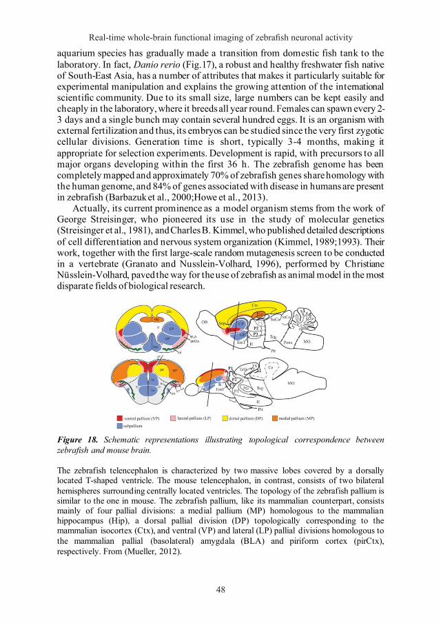
Real-time whole-brain functional imaging of zebrafish neuronal activity
48
aquarium species has gradually made a transition from domestic fish tank to the laboratory. In fact, Danio rerio (Fig.17), a robust and healthy freshwater fish native of South-East Asia, has a number of attributes that makes it particularly suitable for experimental manipulation and explains the growing attention of the international scientific community. Due to its small size, large numbers can be kept easily and cheaply in the laboratory, where it breeds all year round. Females can spawn every 2-3 days and a single bunch may contain several hundred eggs. It is an organism with external fertilization and thus, its embryos can be studied since the very first zygotic cellular divisions. Generation time is short, typically 3-4 months, making it appropriate for selection experiments. Development is rapid, with precursors to all major organs developing within the first 36 h. The zebrafish genome has been completely mapped and approximately 70% of zebrafish genes share homology with the human genome, and 84% of genes associated with disease in humans are present in zebrafish (Barbazuk et al., 2000;Howe et al., 2013).
Actually, its current prominence as a model organism stems from the work of George Streisinger, who pioneered its use in the study of molecular genetics (Streisinger et al., 1981), and Charles B. Kimmel, who published detailed descriptions of cell differentiation and nervous system organization (Kimmel, 1989;1993). Their work, together with the first large-scale random mutagenesis screen to be conducted in a vertebrate (Granato and Nusslein-Volhard, 1996), performed by Christiane Nüsslein-Volhard, paved the way for the use of zebrafish as animal model in the most disparate fields of biological research.
Figure 18. Schematic representations illustrating topological correspondence between zebrafish and mouse brain.
The zebrafish telencephalon is characterized by two massive lobes covered by a dorsally located T-shaped ventricle. The mouse telencephalon, in contrast, consists of two bilateral hemispheres surrounding centrally located ventricles. The topology of the zebrafish pallium is similar to the one in mouse. The zebrafish pallium, like its mammalian counterpart, consists mainly of four pallial divisions: a medial pallium (MP) homologous to the mammalian hippocampus (Hip), a dorsal pallial division (DP) topologically corresponding to the mammalian isocortex (Ctx), and ventral (VP) and lateral (LP) pallial divisions homologous to the mammalian pallial (basolateral) amygdala (BLA) and piriform cortex (pirCtx), respectively. From (Mueller, 2012).
49
In the field of neuroscience, five are the key features that have made zebrafish a particularly interesting and suitable model. First, the CNS of a 3 days post fertilization (dpf) zebrafish larva (Fig. 10) counts approximately 100˙000 neurons (Naumann et al., 2010), which makes it a relatively complex system to be studied if compared to the CNS of invertebrate animal models (e.g. Caernorabditis elegans, Drosophila melanogaster, etc.), but still a simpler and more accessible structure compared to higher vertebrates (e.g. rodents, primates, etc.). Second, zebrafish shares the common neurotransmitters pool with mammals and have similar neuroanatomy in many areas (e.g. retina, hindbrain, spinal cord, etc.). Additionally, due to the different neuro-morphogenesis with respect to mammals13, important nuclei, instead of being in deep and hardly accessible regions as happens in the mammalian brain, become in zebrafish the most superficial, and thus accessible, structures. Indeed, while behaviourally relevant nuclei (e.g. hippocampus, habenula, amygdala, etc.) are difficult regions to reach in mammals due to their deep location beneath the neocortex, in the zebrafish brain these regions (or their functional analogous) are the most dorsal of the telencephalon (Fig.18).
Third, larvae are completely transparent during embryonic development; this means that, in contrast with higher vertebrates, their entire nervous system is optically accessible and can be thus investigated using advanced fluorescence microscopy techniques. State of the art light-sheet microscopy, for example, allows nowadays imaging the entire larval brain (800x600x200 µm3) with single neuron resolution, at a volumetric rate of 12 Hz (Tomer et al., 2015), a more than optimal sampling frequency considering the “slow” kinetics of currently available calcium indicators. Fourth, larval zebrafish, usually within 5 dpf, already exhibit complex behaviours (e.g. food seeking, pray capturing, escape response, etc.) (Kimmel et al., 1995;Kalueff et al., 2013), allowing the study of neuronal activity associated with a specific behaviour. Fifth, but not less important, zebrafish genome can be modified way more easily with respect to other model organisms: the possibility of either producing mutant lines carrying, on orthologue genes, human mutations associated with a pathologic phenotype, or generating transgenic lines expressing fluorescent tags or indicators in a cell-type specific way, dramatically expands the experimental panorama.
Since the early days of using zebrafish as an experimental model, and until relatively recently, nervous system development has been a major focus for research (Hatta and Kimmel, 1993;Blader and Strahle, 2000;Mione et al., 2008;Abraham et al., 2009). Kimmel and colleagues (Kimmel, 1993;Kimmel et al., 1995) performed fine observations of both wild type embryos, having regular neuronal development, and mutant ones, showing aberrant neuro-morphogenesis. With this approach, they provided a detailed and comprehensive description of nervous system organization, unveiling several mechanisms underlying brain morphogenesis. In recent years, the development of tools providing optical readout of neuronal activity and novel imaging techniques moved research focus to the study of neuronal activity and neural circuits function. The genetic targeting of Ca2+ indicators (see Genetically encoded Ca2+
13 Indeed, while the anterior neural tube of mammals undergoes invagination during development (inversion), leading to the deep location of many important nuclei, the zebrafish brain develops by eversion.
48

Lapo Turrini
48
aquarium species has gradually made a transition from domestic fish tank to the laboratory. In fact, Danio rerio (Fig.17), a robust and healthy freshwater fish native of South-East Asia, has a number of attributes that makes it particularly suitable for experimental manipulation and explains the growing attention of the international scientific community. Due to its small size, large numbers can be kept easily and cheaply in the laboratory, where it breeds all year round. Females can spawn every 2-3 days and a single bunch may contain several hundred eggs. It is an organism with external fertilization and thus, its embryos can be studied since the very first zygotic cellular divisions. Generation time is short, typically 3-4 months, making it appropriate for selection experiments. Development is rapid, with precursors to all major organs developing within the first 36 h. The zebrafish genome has been completely mapped and approximately 70% of zebrafish genes share homology with the human genome, and 84% of genes associated with disease in humans are present in zebrafish (Barbazuk et al., 2000;Howe et al., 2013).
Actually, its current prominence as a model organism stems from the work of George Streisinger, who pioneered its use in the study of molecular genetics (Streisinger et al., 1981), and Charles B. Kimmel, who published detailed descriptions of cell differentiation and nervous system organization (Kimmel, 1989;1993). Their work, together with the first large-scale random mutagenesis screen to be conducted in a vertebrate (Granato and Nusslein-Volhard, 1996), performed by Christiane Nüsslein-Volhard, paved the way for the use of zebrafish as animal model in the most disparate fields of biological research.
Figure 18. Schematic representations illustrating topological correspondence between zebrafish and mouse brain.
The zebrafish telencephalon is characterized by two massive lobes covered by a dorsally located T-shaped ventricle. The mouse telencephalon, in contrast, consists of two bilateral hemispheres surrounding centrally located ventricles. The topology of the zebrafish pallium is similar to the one in mouse. The zebrafish pallium, like its mammalian counterpart, consists mainly of four pallial divisions: a medial pallium (MP) homologous to the mammalian hippocampus (Hip), a dorsal pallial division (DP) topologically corresponding to the mammalian isocortex (Ctx), and ventral (VP) and lateral (LP) pallial divisions homologous to the mammalian pallial (basolateral) amygdala (BLA) and piriform cortex (pirCtx), respectively. From (Mueller, 2012).
49
In the field of neuroscience, five are the key features that have made zebrafish a particularly interesting and suitable model. First, the CNS of a 3 days post fertilization (dpf) zebrafish larva (Fig. 10) counts approximately 100˙000 neurons (Naumann et al., 2010), which makes it a relatively complex system to be studied if compared to the CNS of invertebrate animal models (e.g. Caernorabditis elegans, Drosophila melanogaster, etc.), but still a simpler and more accessible structure compared to higher vertebrates (e.g. rodents, primates, etc.). Second, zebrafish shares the common neurotransmitters pool with mammals and have similar neuroanatomy in many areas (e.g. retina, hindbrain, spinal cord, etc.). Additionally, due to the different neuro-morphogenesis with respect to mammals13, important nuclei, instead of being in deep and hardly accessible regions as happens in the mammalian brain, become in zebrafish the most superficial, and thus accessible, structures. Indeed, while behaviourally relevant nuclei (e.g. hippocampus, habenula, amygdala, etc.) are difficult regions to reach in mammals due to their deep location beneath the neocortex, in the zebrafish brain these regions (or their functional analogous) are the most dorsal of the telencephalon (Fig.18).
Third, larvae are completely transparent during embryonic development; this means that, in contrast with higher vertebrates, their entire nervous system is optically accessible and can be thus investigated using advanced fluorescence microscopy techniques. State of the art light-sheet microscopy, for example, allows nowadays imaging the entire larval brain (800x600x200 µm3) with single neuron resolution, at a volumetric rate of 12 Hz (Tomer et al., 2015), a more than optimal sampling frequency considering the “slow” kinetics of currently available calcium indicators. Fourth, larval zebrafish, usually within 5 dpf, already exhibit complex behaviours (e.g. food seeking, pray capturing, escape response, etc.) (Kimmel et al., 1995;Kalueff et al., 2013), allowing the study of neuronal activity associated with a specific behaviour. Fifth, but not less important, zebrafish genome can be modified way more easily with respect to other model organisms: the possibility of either producing mutant lines carrying, on orthologue genes, human mutations associated with a pathologic phenotype, or generating transgenic lines expressing fluorescent tags or indicators in a cell-type specific way, dramatically expands the experimental panorama.
Since the early days of using zebrafish as an experimental model, and until relatively recently, nervous system development has been a major focus for research (Hatta and Kimmel, 1993;Blader and Strahle, 2000;Mione et al., 2008;Abraham et al., 2009). Kimmel and colleagues (Kimmel, 1993;Kimmel et al., 1995) performed fine observations of both wild type embryos, having regular neuronal development, and mutant ones, showing aberrant neuro-morphogenesis. With this approach, they provided a detailed and comprehensive description of nervous system organization, unveiling several mechanisms underlying brain morphogenesis. In recent years, the development of tools providing optical readout of neuronal activity and novel imaging techniques moved research focus to the study of neuronal activity and neural circuits function. The genetic targeting of Ca2+ indicators (see Genetically encoded Ca2+
13 Indeed, while the anterior neural tube of mammals undergoes invagination during development (inversion), leading to the deep location of many important nuclei, the zebrafish brain develops by eversion.
49

Real-time whole-brain functional imaging of zebrafish neuronal activity
50
indicators) in all neurons of the zebrafish larva opened the way to the unprecedented non-invasive in vivo functional investigation of a vertebrate brain in its entirety (Ahrens et al., 2013;Panier et al., 2013) (Fig.19). Ahrens and colleagues (Ahrens et al., 2013) first applied fast light-sheet microscopy to perform real-time brain-wide imaging (800x600x200 µm3) of restrained zebrafish larvae, at a volumetric framerate of 0.8 Hz. Indeed, currently available technology, coupled to last generation GECIs, allowed Tomer et al. (Tomer et al., 2015) to perform functional light-sheet imaging of the entire larval CNS (3000x500x200 µm3) at a sampling rate of more than 6 Hz (Fig.19). Whole-brain imaging has been proficiently applied to the identification of functional circuitry while head-restrained fictively behaving larvae were exposed to virtual environment stimulation (Freeman et al., 2014;Portugues et al., 2014;Vladimirov et al., 2014;Dunn et al., 2016a;Dunn et al., 2016b;Guggiana-Nilo and Engert, 2016;Naumann et al., 2016;Haesemeyer et al., 2018). In particular, Vladimirov and colleagues (Vladimirov et al., 2014) first, using light-sheet microscopy, measured neuronal activity during optomotor response in larvae exposed to a moving grating visual pattern (Fig.20). The same virtual reality experimental paradigm allowed Freeman and colleagues (Freeman et al., 2014) to produce whole brain maps showing the tuning of individual neurons in response to the different moving directions of the visual stimulus presented (Fig.20). Portugues et al. (Portugues et al., 2014), performing whole brain light-sheet imaging in larvae to which a rotating grating visual pattern was presented, identified a broadly distributed stereotyped functional network governing the optokinetic response (Fig.20). Dunn et al. (Dunn et al., 2016b), studying the exploratory behaviour of freely swimming larvae in absence of salient sensory cue, found that their trajectories were characterized by alternating sequences of repeated turns (Fig.20). In parallel, performing brain-wide light-sheet imaging of fictively behaving larvae, they identified specific neural populations whose activity controlled the observed behaviour (Fig.20). Recently, in the effort to measure larval neuronal activity in conditions closer to the physiological ones, two groups (Cong et al., 2017;Kim et al., 2017) have applied the principle of light field microscopy (LFM) to perform whole-brain functional imaging in freely swimming larvae. In particular, Kim and colleagues (Kim et al., 2017), coupling LFM with structured illumination and a newly developed motion-cancellation custom system, were able to image with cellular resolution the entire brain of freely moving larvae exposed to thermal stimuli (heat avoidance behaviour) (Fig.21). The novel concept they have devised dramatically expands the behavioural repertoire amenable to brain-wide cellular-resolution imaging, potentially including spatial navigation, social behaviour, feeding or reward. Owing to technological improvement and development of novel microscopes, built around the specimen and capable of faster volumetric acquisition, the zebrafish, with its unique features, represents an excellent vertebrate model to study the nervous system, in the attempt to disentangle and understand the functional circuitry and neuronal activity patterns at the base of specific behaviours.
51
Figure 19. Whole-brain functional imaging in zebrafish.
Milestone publications about brain-wide functional imaging in restrained zebrafish larvae.
50
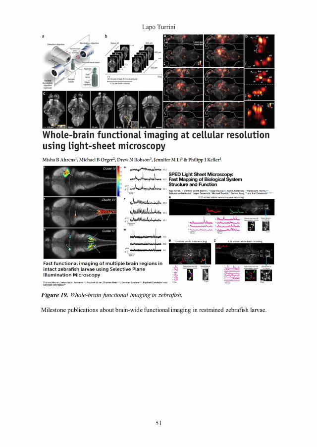
Lapo Turrini
50
indicators) in all neurons of the zebrafish larva opened the way to the unprecedented non-invasive in vivo functional investigation of a vertebrate brain in its entirety (Ahrens et al., 2013;Panier et al., 2013) (Fig.19). Ahrens and colleagues (Ahrens et al., 2013) first applied fast light-sheet microscopy to perform real-time brain-wide imaging (800x600x200 µm3) of restrained zebrafish larvae, at a volumetric framerate of 0.8 Hz. Indeed, currently available technology, coupled to last generation GECIs, allowed Tomer et al. (Tomer et al., 2015) to perform functional light-sheet imaging of the entire larval CNS (3000x500x200 µm3) at a sampling rate of more than 6 Hz (Fig.19). Whole-brain imaging has been proficiently applied to the identification of functional circuitry while head-restrained fictively behaving larvae were exposed to virtual environment stimulation (Freeman et al., 2014;Portugues et al., 2014;Vladimirov et al., 2014;Dunn et al., 2016a;Dunn et al., 2016b;Guggiana-Nilo and Engert, 2016;Naumann et al., 2016;Haesemeyer et al., 2018). In particular, Vladimirov and colleagues (Vladimirov et al., 2014) first, using light-sheet microscopy, measured neuronal activity during optomotor response in larvae exposed to a moving grating visual pattern (Fig.20). The same virtual reality experimental paradigm allowed Freeman and colleagues (Freeman et al., 2014) to produce whole brain maps showing the tuning of individual neurons in response to the different moving directions of the visual stimulus presented (Fig.20). Portugues et al. (Portugues et al., 2014), performing whole brain light-sheet imaging in larvae to which a rotating grating visual pattern was presented, identified a broadly distributed stereotyped functional network governing the optokinetic response (Fig.20). Dunn et al. (Dunn et al., 2016b), studying the exploratory behaviour of freely swimming larvae in absence of salient sensory cue, found that their trajectories were characterized by alternating sequences of repeated turns (Fig.20). In parallel, performing brain-wide light-sheet imaging of fictively behaving larvae, they identified specific neural populations whose activity controlled the observed behaviour (Fig.20). Recently, in the effort to measure larval neuronal activity in conditions closer to the physiological ones, two groups (Cong et al., 2017;Kim et al., 2017) have applied the principle of light field microscopy (LFM) to perform whole-brain functional imaging in freely swimming larvae. In particular, Kim and colleagues (Kim et al., 2017), coupling LFM with structured illumination and a newly developed motion-cancellation custom system, were able to image with cellular resolution the entire brain of freely moving larvae exposed to thermal stimuli (heat avoidance behaviour) (Fig.21). The novel concept they have devised dramatically expands the behavioural repertoire amenable to brain-wide cellular-resolution imaging, potentially including spatial navigation, social behaviour, feeding or reward. Owing to technological improvement and development of novel microscopes, built around the specimen and capable of faster volumetric acquisition, the zebrafish, with its unique features, represents an excellent vertebrate model to study the nervous system, in the attempt to disentangle and understand the functional circuitry and neuronal activity patterns at the base of specific behaviours.
51
Figure 19. Whole-brain functional imaging in zebrafish.
Milestone publications about brain-wide functional imaging in restrained zebrafish larvae.
51

Real-time whole-brain functional imaging of zebrafish neuronal activity
52
Figure 20. Whole-brain functional imaging in fictively behaving zebrafish.
Key publications applying the whole-brain functional imaging to partially restrained zebrafish larvae during virtual reality experiments.
53
Figure 21. Whole-brain functional imaging in freely swimming zebrafish.
Most recent technology breakthroughs allowed the whole-brain measurements in freely behaving zebrafish larvae.
52

Lapo Turrini
52
Figure 20. Whole-brain functional imaging in fictively behaving zebrafish.
Key publications applying the whole-brain functional imaging to partially restrained zebrafish larvae during virtual reality experiments.
53
Figure 21. Whole-brain functional imaging in freely swimming zebrafish.
Most recent technology breakthroughs allowed the whole-brain measurements in freely behaving zebrafish larvae.
53
Real-time whole-brain functional imaging of zebrafish neuronal activity
54
7.1 Zebrafish and epilepsy
Epilepsy14 is the most common and widespread neurological disorder characterized by aberrant cerebral activity in humans. This pathology is characterized by recurrent and unprovoked spontaneous bursts of neuronal activity, known as seizures, which are linked to a loss of balance between excitatory and inhibitory synapses. The aetiology of epilepsy is manifold, ranging from genetic mutations affecting membrane ion channels (Noebels, 2003), altering neuronal migration, or protein degradation in neurons (Olson et al., 2014), to a variety of insults, such as brain tumours, injury, stroke or neurodegeneration. Despite a wide range of anti-epileptic drugs (AEDs) currently available for treatment of epilepsy (Stafstorm, 2010), approximately 35% of patients fail to respond adequately to therapy (Go and Snead, 2008;Ernst and Boudreau, 2016). Typically, most of the research on AEDs is performed using rodent models. These models have significantly contributed to increase our comprehension of epilepsy but suffer from limitations for the identification of new AEDs, regarding, for example, the throughput of drug screening and the time required to generate new transgenic lines to model specific epileptic pathogenic mechanisms. In recent years, zebrafish has rapidly emerged as a valid animal model to study this pathology both in basic research and in drug discovery. Indeed, owing to the features discussed in the previous session, zebrafish represents a key animal model to study epilepsy from a perspective not applicable with mammals. Seizures can be easily induced in zebrafish using pentylenetetrazole15 (PTZ), a molecule that recent studies revealed can be successfully used to model seizure-like behaviour in zebrafish larvae, making this pharmacological approach suitable to study several kinds of human epilepsy in this animal model (Baraban et al., 2005;Stewart et al., 2012). Thus far, epileptic seizures have been detected and characterized in zebrafish either as behavioural alterations or by means of direct electrographic recordings. Behavioural measurements rely on the recording of swimming activity by time-lapse videos and tracking of the larva position in time (Baraban et al., 2005;Winter et al., 2008;Afrikanova et al., 2013). During seizures, larvae exhibit a variety of behaviours classified in different epileptic stages (Baraban et al., 2005). This type of measurements has been used to characterize chemically induced convulsions and to screen potential anti-convulsant drugs, capable of reversing the effects of PTZ (Dinday and Baraban, 2015). However, a detailed study of the mechanisms of epilepsy requires measuring the neuronal activity underlying seizures. The most used method to this end is the electrographic recording of activity in large areas of the larval brain via extracellular field recordings. These studies have proved effective in detecting brain electrical activity and its alterations, which correlate with seizures (Baraban et al., 2005;Afrikanova et al., 2013;Zdebik et
14 This neurological disorder was already known by the ancients. The first recorded report traces back to an Assyrian text (2000 B.C.). Hippocrates (400 B.C.), in his On the Sacred Disease, gives one of the first accurate description of the pathology, making conjectures about its probable aetiology (Magiorkinis et al., 2010). 15 Pentylenetetrazole is a molecule that is thought, based on binding studies, to act as a competitive inhibitor at the picrotoxin site of the γ-aminobutyric acid type A (GABAA) receptor. PTZ inhibits the GABA-activated iperpolarizing Cl- current in a concentration dependent manner, thus reducing the inhibitory effects of GABA signalling (Huang et al., 2001).
55
al., 2013), despite lacking in spatial resolution. Indeed, the use of the novel optical methods discussed previously (see Genetically encoded Ca2+ indicators) applied to the study of epilepsy, could provide new insights regarding the mechanisms underlying the onset of aberrant electrical activity characterizing this pathology.
54

Lapo Turrini
54
7.1 Zebrafish and epilepsy
Epilepsy14 is the most common and widespread neurological disorder characterized by aberrant cerebral activity in humans. This pathology is characterized by recurrent and unprovoked spontaneous bursts of neuronal activity, known as seizures, which are linked to a loss of balance between excitatory and inhibitory synapses. The aetiology of epilepsy is manifold, ranging from genetic mutations affecting membrane ion channels (Noebels, 2003), altering neuronal migration, or protein degradation in neurons (Olson et al., 2014), to a variety of insults, such as brain tumours, injury, stroke or neurodegeneration. Despite a wide range of anti-epileptic drugs (AEDs) currently available for treatment of epilepsy (Stafstorm, 2010), approximately 35% of patients fail to respond adequately to therapy (Go and Snead, 2008;Ernst and Boudreau, 2016). Typically, most of the research on AEDs is performed using rodent models. These models have significantly contributed to increase our comprehension of epilepsy but suffer from limitations for the identification of new AEDs, regarding, for example, the throughput of drug screening and the time required to generate new transgenic lines to model specific epileptic pathogenic mechanisms. In recent years, zebrafish has rapidly emerged as a valid animal model to study this pathology both in basic research and in drug discovery. Indeed, owing to the features discussed in the previous session, zebrafish represents a key animal model to study epilepsy from a perspective not applicable with mammals. Seizures can be easily induced in zebrafish using pentylenetetrazole15 (PTZ), a molecule that recent studies revealed can be successfully used to model seizure-like behaviour in zebrafish larvae, making this pharmacological approach suitable to study several kinds of human epilepsy in this animal model (Baraban et al., 2005;Stewart et al., 2012). Thus far, epileptic seizures have been detected and characterized in zebrafish either as behavioural alterations or by means of direct electrographic recordings. Behavioural measurements rely on the recording of swimming activity by time-lapse videos and tracking of the larva position in time (Baraban et al., 2005;Winter et al., 2008;Afrikanova et al., 2013). During seizures, larvae exhibit a variety of behaviours classified in different epileptic stages (Baraban et al., 2005). This type of measurements has been used to characterize chemically induced convulsions and to screen potential anti-convulsant drugs, capable of reversing the effects of PTZ (Dinday and Baraban, 2015). However, a detailed study of the mechanisms of epilepsy requires measuring the neuronal activity underlying seizures. The most used method to this end is the electrographic recording of activity in large areas of the larval brain via extracellular field recordings. These studies have proved effective in detecting brain electrical activity and its alterations, which correlate with seizures (Baraban et al., 2005;Afrikanova et al., 2013;Zdebik et
14 This neurological disorder was already known by the ancients. The first recorded report traces back to an Assyrian text (2000 B.C.). Hippocrates (400 B.C.), in his On the Sacred Disease, gives one of the first accurate description of the pathology, making conjectures about its probable aetiology (Magiorkinis et al., 2010). 15 Pentylenetetrazole is a molecule that is thought, based on binding studies, to act as a competitive inhibitor at the picrotoxin site of the γ-aminobutyric acid type A (GABAA) receptor. PTZ inhibits the GABA-activated iperpolarizing Cl- current in a concentration dependent manner, thus reducing the inhibitory effects of GABA signalling (Huang et al., 2001).
55
al., 2013), despite lacking in spatial resolution. Indeed, the use of the novel optical methods discussed previously (see Genetically encoded Ca2+ indicators) applied to the study of epilepsy, could provide new insights regarding the mechanisms underlying the onset of aberrant electrical activity characterizing this pathology.
55

57
Part II
Methods
56

57
Part II
Methods

59
Chapter 8 Generation of the GCaMP6s transgenic zebrafish line
Aiming to produce a transgenic zebrafish line expressing in the nucleus of all CNS neurons the fast and sensitive Ca2+ reporter GCaMP6s (Chen et al., 2013), we chose the plasmid tol2-elavl3:H2B-GCaMP6s (Addgene, Cambridge, Massachusetts, USA) (Freeman et al., 2014). The 14288 bp vector (Fig.22) carries the GCaMP6s gene fused with histone H2B gene, under the control of elavl3 promoter.
Figure 22. Map of the tol2-elavl3:H2B-GCaMP6s plasmid.
The transgene GCaMP6s is fused to the histone H2B gene, and this fusion gene is placed downstream to the pan-neuronal promoter elavl3 (here HuC). The expression cassette is flanked by two consensus sequences (brown triangles). The plasmid backbone carries the ampicillin resistance gene AmpR.
58

59
Chapter 8 Generation of the GCaMP6s transgenic zebrafish line
Aiming to produce a transgenic zebrafish line expressing in the nucleus of all CNS neurons the fast and sensitive Ca2+ reporter GCaMP6s (Chen et al., 2013), we chose the plasmid tol2-elavl3:H2B-GCaMP6s (Addgene, Cambridge, Massachusetts, USA) (Freeman et al., 2014). The 14288 bp vector (Fig.22) carries the GCaMP6s gene fused with histone H2B gene, under the control of elavl3 promoter.
Figure 22. Map of the tol2-elavl3:H2B-GCaMP6s plasmid.
The transgene GCaMP6s is fused to the histone H2B gene, and this fusion gene is placed downstream to the pan-neuronal promoter elavl3 (here HuC). The expression cassette is flanked by two consensus sequences (brown triangles). The plasmid backbone carries the ampicillin resistance gene AmpR. Lapo Turrini, Development of optical methods for real-time whole-brain functional imaging of zebrafish neuronal activity, © 2020 Author(s), content CC BY 4.0 International, metadata CC0 1.0 Universal, published by Firenze University Press (www.fupress.com), ISSN 2612-8020 (online), ISBN 978-88-5518-070-2 (PDF), DOI 10.36253/978-88-5518-070-2

Real-time whole-brain functional imaging of zebrafish neuronal activity
60
The insert is flanked by two consensus sequences specifically recognized by the Tol2 transposase. The expression product is a fusion protein H2B-GCaMP6s, which guarantees the nuclear localization of the reporter, present in all differentiated neurons owing to the elavl3 promoter. The most common method to obtain a transgenic zebrafish line, is to microinject the plasmid carrying the insert into fertilized eggs, together with Tol2 transcript (Kawakami, 2007). Once inside the zygote, the translational apparatus of the embryo translates Tol2 mRNA into the active Tol2 transposase. The enzyme binds the tol2 consensus sequences and excises the insert, performing a random recombination with the genomic DNA.
8.1 Amplification of plasmid tol2-elavl3:H2B-GCaMP6s
We first proceeded to amplify tol2-elavl3:H2B-GCaMP6s plasmid (carrying resistance to ampicillin as a marker for selection), performing a heat-shock bacterial transformation followed by growth of transformed cells and plasmid purification.
8.1.1 Bacterial transformation with tol2-elavl3:H2B-GCaMP6s plasmid
To perform bacterial transformation, a 50 µL aliquot of DH5α E. coli competent cells, stored at -80 °C, was thawed on ice. 25 ng of plasmid (1 µL) were added to the tube and the solution was gently mixed with a pipette tip. The competent cells/plasmid mixture was then incubated on ice for 30 minutes. The cells were then heat shocked in a 42 °C water bath for 45 seconds. The tube was put back on ice for 2 minutes; 250 µL of pre-warmed (37 °C) sterile LB16 liquid medium were gently mixed with the bacteria. The transformation tube was placed in a shaking incubator (200 rpm) at 37 °C for 30 minutes. This first growth step allows bacteria to generate the ampicillin resistance proteins encoded in the plasmid backbone, so that they will be able to grow once plated onto agar plates containing the antibiotic. After this incubation, the bacterial solution was plated using a sterile spreader onto 10 cm plates containing LB 1.5 % agar added with 100 ng/mL ampicillin17. The plates were incubated at 37 °C overnight.
8.1.2 tol2-elavl3:H2B-GCaMP6s plasmid extraction
Since only bacteria that incorporated the plasmid produce ampicillin resistance proteins and are thus able to grow onto medium containing the antibiotic, we could select a single colony grown to be sure to recover only clones of a transformed bacterium. The colony was isolated from the medium surface using a sterile loop and
16 The lysogeny broth (LB) was prepared dissolving 10 g tryptone (T7293, Sigma-Aldrich, Saint Louis, Missouri, USA), 5 g yeast extract (70161, Sigma-Aldrich, Saint Louis, Missouri, USA) and 10 g NaCl into 800 mL ddH2O. pH of solution was balanced around 7 and final volume brought to 1000 mL. LB medium was sterilized in autoclave (15 min at 121 °C). 17 LB 1.5 % solid medium was prepared melting bacteriological agar (A5306, Sigma-Aldrich, Saint Louis, Missouri, USA) into liquid LB medium. Once cooled down to 60 °C the still liquid medium was added with 1 µL/mL ampicillin [100 ng/ µL].
61
then inoculated into a 2 mL sterile LB liquid medium starter culture supplemented with 100 ng/mL ampicillin). The vial containing the starter culture was placed in a shaking incubator (300 rpm) at 37 °C for 8 hours. Terminated the incubation, 100 µL of starter culture were diluted into 100 mL of sterile LB liquid medium added with 100 ng/mL ampicillin. The solution was placed in a 500 mL flask on a shaking incubator (300 rpm) at 37 °C overnight. At the end of the incubation, the tol2-elavl3:H2B-GCaMP6s plasmid was purified using the QIAGEN Plasmid Midi kit (12123, QIAGEN, Hilden, Germany).
8.2 In vitro transcription of tol2 plasmid
To obtain the Tol2 transposase mRNA, necessary in the microinjection procedure in order for the insert to be integrated in the zebrafish embryo genome, we set up an in vitro transcription reaction of the pCS2-TP plasmid using the reliable mMESSAGE mMACHINE SP6 Transcription kit (AM1340, Ambion, Life Technologies, Carlsbad, California, USA). All procedures were performed using RNase-free supplies. Indeed, even low concentration of nucleases can degrade the transcript.
The first step, to allow SP6 polymerase to operate the transcription, was to linearize the plasmid through an enzymatic digestion using NotI, as its restriction site is present only once in the plasmid sequence. Restriction reaction was performed adding in a tube the reagents as follow: 19 µL dIH2O, 5 µL 3.1 buffer (B7203S, New England Biolobs, Ipswich, Massachussetts, USA), 6 µg pCS2-TP plasmid (24 µL at 260 ng/µL) and 2 µL NotI enzyme (R0189, New England Biolobs, Ipswich, Massachussetts, USA) to arrive at a final volume of 50 µL. The tube was incubated at 37 °C overnight. The restriction reaction was terminated, and the DNA precipitated by adding 2.5 µL 0.5 M EDTA, 5 µL 5M ammonium acetate and 100 µL absolute ethanol. The solution was mixed and cooled down to -20 °C for 165 minutes. The tube was then centrifuged (benchtop centrifuge 5417R, Eppendorf, Hamburg, Germany) for 15 min at maximum speed. The supernatant was discarded, and the tube centrifuged again for a few seconds to remove the residual fluid. The linearized plasmid pellet was resuspended in 12 µL dIH2O at a final concentration of 455 ng/ µL (as determined by reading absorbance at 260 nm with the spectrophotometer NanoVue Plus, GE Healthcare, Chicago Illinois, USA).
The linearized plasmid solution was then used as a substrate for the in vitro transcription kit. At the end of the transcription reaction, the mRNA was recovered using the RNA Clean & Concentrator-5 (R1015, Zymo Research, Irvine, California, USA). The final yield was ~21.4 µg of mRNA (30 µL at 713 ng/µL) as determined by reading absorbance at 260 nm. The transcript was diluted on ice at 125 ng/µL and stored at -80 °C in 2 µL aliquots in 500 µL reaction tubes.
8.3 Microinjection
As the zebrafish natural behaviour is to mate at dawn, the zebrafish facility is equipped with a temporized illumination system that ramps up lights at 9 am for our
60

Lapo Turrini
60
The insert is flanked by two consensus sequences specifically recognized by the Tol2 transposase. The expression product is a fusion protein H2B-GCaMP6s, which guarantees the nuclear localization of the reporter, present in all differentiated neurons owing to the elavl3 promoter. The most common method to obtain a transgenic zebrafish line, is to microinject the plasmid carrying the insert into fertilized eggs, together with Tol2 transcript (Kawakami, 2007). Once inside the zygote, the translational apparatus of the embryo translates Tol2 mRNA into the active Tol2 transposase. The enzyme binds the tol2 consensus sequences and excises the insert, performing a random recombination with the genomic DNA.
8.1 Amplification of plasmid tol2-elavl3:H2B-GCaMP6s
We first proceeded to amplify tol2-elavl3:H2B-GCaMP6s plasmid (carrying resistance to ampicillin as a marker for selection), performing a heat-shock bacterial transformation followed by growth of transformed cells and plasmid purification.
8.1.1 Bacterial transformation with tol2-elavl3:H2B-GCaMP6s plasmid
To perform bacterial transformation, a 50 µL aliquot of DH5α E. coli competent cells, stored at -80 °C, was thawed on ice. 25 ng of plasmid (1 µL) were added to the tube and the solution was gently mixed with a pipette tip. The competent cells/plasmid mixture was then incubated on ice for 30 minutes. The cells were then heat shocked in a 42 °C water bath for 45 seconds. The tube was put back on ice for 2 minutes; 250 µL of pre-warmed (37 °C) sterile LB16 liquid medium were gently mixed with the bacteria. The transformation tube was placed in a shaking incubator (200 rpm) at 37 °C for 30 minutes. This first growth step allows bacteria to generate the ampicillin resistance proteins encoded in the plasmid backbone, so that they will be able to grow once plated onto agar plates containing the antibiotic. After this incubation, the bacterial solution was plated using a sterile spreader onto 10 cm plates containing LB 1.5 % agar added with 100 ng/mL ampicillin17. The plates were incubated at 37 °C overnight.
8.1.2 tol2-elavl3:H2B-GCaMP6s plasmid extraction
Since only bacteria that incorporated the plasmid produce ampicillin resistance proteins and are thus able to grow onto medium containing the antibiotic, we could select a single colony grown to be sure to recover only clones of a transformed bacterium. The colony was isolated from the medium surface using a sterile loop and
16 The lysogeny broth (LB) was prepared dissolving 10 g tryptone (T7293, Sigma-Aldrich, Saint Louis, Missouri, USA), 5 g yeast extract (70161, Sigma-Aldrich, Saint Louis, Missouri, USA) and 10 g NaCl into 800 mL ddH2O. pH of solution was balanced around 7 and final volume brought to 1000 mL. LB medium was sterilized in autoclave (15 min at 121 °C). 17 LB 1.5 % solid medium was prepared melting bacteriological agar (A5306, Sigma-Aldrich, Saint Louis, Missouri, USA) into liquid LB medium. Once cooled down to 60 °C the still liquid medium was added with 1 µL/mL ampicillin [100 ng/ µL].
61
then inoculated into a 2 mL sterile LB liquid medium starter culture supplemented with 100 ng/mL ampicillin). The vial containing the starter culture was placed in a shaking incubator (300 rpm) at 37 °C for 8 hours. Terminated the incubation, 100 µL of starter culture were diluted into 100 mL of sterile LB liquid medium added with 100 ng/mL ampicillin. The solution was placed in a 500 mL flask on a shaking incubator (300 rpm) at 37 °C overnight. At the end of the incubation, the tol2-elavl3:H2B-GCaMP6s plasmid was purified using the QIAGEN Plasmid Midi kit (12123, QIAGEN, Hilden, Germany).
8.2 In vitro transcription of tol2 plasmid
To obtain the Tol2 transposase mRNA, necessary in the microinjection procedure in order for the insert to be integrated in the zebrafish embryo genome, we set up an in vitro transcription reaction of the pCS2-TP plasmid using the reliable mMESSAGE mMACHINE SP6 Transcription kit (AM1340, Ambion, Life Technologies, Carlsbad, California, USA). All procedures were performed using RNase-free supplies. Indeed, even low concentration of nucleases can degrade the transcript.
The first step, to allow SP6 polymerase to operate the transcription, was to linearize the plasmid through an enzymatic digestion using NotI, as its restriction site is present only once in the plasmid sequence. Restriction reaction was performed adding in a tube the reagents as follow: 19 µL dIH2O, 5 µL 3.1 buffer (B7203S, New England Biolobs, Ipswich, Massachussetts, USA), 6 µg pCS2-TP plasmid (24 µL at 260 ng/µL) and 2 µL NotI enzyme (R0189, New England Biolobs, Ipswich, Massachussetts, USA) to arrive at a final volume of 50 µL. The tube was incubated at 37 °C overnight. The restriction reaction was terminated, and the DNA precipitated by adding 2.5 µL 0.5 M EDTA, 5 µL 5M ammonium acetate and 100 µL absolute ethanol. The solution was mixed and cooled down to -20 °C for 165 minutes. The tube was then centrifuged (benchtop centrifuge 5417R, Eppendorf, Hamburg, Germany) for 15 min at maximum speed. The supernatant was discarded, and the tube centrifuged again for a few seconds to remove the residual fluid. The linearized plasmid pellet was resuspended in 12 µL dIH2O at a final concentration of 455 ng/ µL (as determined by reading absorbance at 260 nm with the spectrophotometer NanoVue Plus, GE Healthcare, Chicago Illinois, USA).
The linearized plasmid solution was then used as a substrate for the in vitro transcription kit. At the end of the transcription reaction, the mRNA was recovered using the RNA Clean & Concentrator-5 (R1015, Zymo Research, Irvine, California, USA). The final yield was ~21.4 µg of mRNA (30 µL at 713 ng/µL) as determined by reading absorbance at 260 nm. The transcript was diluted on ice at 125 ng/µL and stored at -80 °C in 2 µL aliquots in 500 µL reaction tubes.
8.3 Microinjection
As the zebrafish natural behaviour is to mate at dawn, the zebrafish facility is equipped with a temporized illumination system that ramps up lights at 9 am for our
61

Real-time whole-brain functional imaging of zebrafish neuronal activity
62
convenience, producing an artificial dawn. To prepare the in jection mix a 500 µL reaction tube containing 2 µL Tol2 mRNA at 125 ng/µL, kept at -80 °C, was placed on ice. Reagents were then added to the tube as follows: 6 µL ddH2O, 1 µL 1% w/v phenol red18 (P3532, Sigma-Aldrich, Saint Louis, Missouri, USA) and 1 µL tol2-elavl3:H2B-GCaMP6s plasmid at a concentration of 250 ng/µL, with 10 µL final volume. The tube was first vortexed to make the solution homogeneous, then spinned briefly to collect the whole injection mix at its bottom, and finally placed back on ice.
The fine needles used to microinject zebrafish eggs were derived from glass capillaries (O.D. 1.0 mm, I.D. 0.5 mm, length 10 cm; BF100-50-10, Sutter Instrument, Novato, California, USA) through the same pulling process used to produce micropipettes for electrophysiology. In order to obtain superfine-tipped needles, yet with the appropriate stiffness, the micropipette puller (P-1000 Flaming/Brown type, Sutter Instrument, Novato, California, USA) was set with the following parameters: heat, 645; pull, 60; velocity, 80. As the injection needles have a closed tip, due to the pulling process, the very end of the needle tip was broken with fine forceps (Dumont #5, Fine Science Tools, Vancouver, Canada).
Typically, 2-3 µL of mix were loaded into a pulled injection needle using a specific electrode loading pipette tip (cat.5242956.003, Eppendorf, Hamburg, Germany), before plugging the needle to the microinjector (FemtoJet 4i, Eppendorf, Hamburg, Germany) holder.
The microinjector was set up with the appropriate pressure and time of injection parameters19 in order to inject the proper volume inside each embryo. As the needle is manually opened, parameters had to be modified from time to time according to the diameter of the needle tip and based on the observed volume of solution injected.
Microinjection procedure consisted in injecting the mix into the yolk of one cell stage wt AB/Tübingen zebrafish embryos. As the injected mix diffuses into the zygote, the translational apparatus of the cell gives rise to the active tol2 transposase, which operates the recombination.
8.4 Transgenic line selection
In order to select embryos expressing the transgene, we performed a fluorescence-based screening. We equipped a stereomicroscope (Stemi 508, Carl Zeiss, Oberkochen, Germany) with a 470 nm blue LED (M470L3, Thorlabs, Dachau, Germany) opportunely filtered (FF01-469/35, Semrock, Rohnert Park, California, USA). Excitation light was blocked with a couple of filters (FF02-525/40, Semrock, Rohnert Park, California, USA) mounted directly into the microscope oculars. Embryos were selected according to the presence of fluorescent signal coming from the CNS.
As the tol2-mediated recombination is a stochastic event, and typically the transposase, as long as it remains active, can also excise the insert out of the genomic DNA, microinjection rarely gives rise to embryos expressing the transgene in all cells
18 Phenol red is used to colour the otherwise transparent mix, in order to visualize the injection location. 19 Typically: injection pressure, 650 hPa; injection time, 0.5 s; compensation pressure, 20 hPa.
63
in which it is supposed to express. Rather, injected embryos are most often a mosaic of expression. For this reason, once reached adulthood (~3-4 months) we performed an outcross between each of the microinjection positive individuals (F0, Fig.23b) and a wt AB/Tübingen zebrafish. In order to select the founders of our transgenic line, we performed a second fluorescence screening on the offspring of each microinjection positive fish. Only zebrafish which integrated the transgene in the germ line gave rise to fluorescent offspring (F1, Fig.23c).
Figure 23. Transgenic line fluorescence screening.
a, b. Wide-field fluorescence images of microinjected F0 larvae showing no fluorescent signal (a) and some sparse labelling (b) arising from the CNS. c. Wide-field fluorescence image of a F1 Tg(elavl3:H2B-GCaMP6s) larva showing brain-wide expression of the fluorescent reporter. Scale bar: 500 µm. The signal arising from the yolk of each of the three larvae is due to auto fluorescence.
62

Lapo Turrini
62
convenience, producing an artificial dawn. To prepare the in jection mix a 500 µL reaction tube containing 2 µL Tol2 mRNA at 125 ng/µL, kept at -80 °C, was placed on ice. Reagents were then added to the tube as follows: 6 µL ddH2O, 1 µL 1% w/v phenol red18 (P3532, Sigma-Aldrich, Saint Louis, Missouri, USA) and 1 µL tol2-elavl3:H2B-GCaMP6s plasmid at a concentration of 250 ng/µL, with 10 µL final volume. The tube was first vortexed to make the solution homogeneous, then spinned briefly to collect the whole injection mix at its bottom, and finally placed back on ice.
The fine needles used to microinject zebrafish eggs were derived from glass capillaries (O.D. 1.0 mm, I.D. 0.5 mm, length 10 cm; BF100-50-10, Sutter Instrument, Novato, California, USA) through the same pulling process used to produce micropipettes for electrophysiology. In order to obtain superfine-tipped needles, yet with the appropriate stiffness, the micropipette puller (P-1000 Flaming/Brown type, Sutter Instrument, Novato, California, USA) was set with the following parameters: heat, 645; pull, 60; velocity, 80. As the injection needles have a closed tip, due to the pulling process, the very end of the needle tip was broken with fine forceps (Dumont #5, Fine Science Tools, Vancouver, Canada).
Typically, 2-3 µL of mix were loaded into a pulled injection needle using a specific electrode loading pipette tip (cat.5242956.003, Eppendorf, Hamburg, Germany), before plugging the needle to the microinjector (FemtoJet 4i, Eppendorf, Hamburg, Germany) holder.
The microinjector was set up with the appropriate pressure and time of injection parameters19 in order to inject the proper volume inside each embryo. As the needle is manually opened, parameters had to be modified from time to time according to the diameter of the needle tip and based on the observed volume of solution injected.
Microinjection procedure consisted in injecting the mix into the yolk of one cell stage wt AB/Tübingen zebrafish embryos. As the injected mix diffuses into the zygote, the translational apparatus of the cell gives rise to the active tol2 transposase, which operates the recombination.
8.4 Transgenic line selection
In order to select embryos expressing the transgene, we performed a fluorescence-based screening. We equipped a stereomicroscope (Stemi 508, Carl Zeiss, Oberkochen, Germany) with a 470 nm blue LED (M470L3, Thorlabs, Dachau, Germany) opportunely filtered (FF01-469/35, Semrock, Rohnert Park, California, USA). Excitation light was blocked with a couple of filters (FF02-525/40, Semrock, Rohnert Park, California, USA) mounted directly into the microscope oculars. Embryos were selected according to the presence of fluorescent signal coming from the CNS.
As the tol2-mediated recombination is a stochastic event, and typically the transposase, as long as it remains active, can also excise the insert out of the genomic DNA, microinjection rarely gives rise to embryos expressing the transgene in all cells
18 Phenol red is used to colour the otherwise transparent mix, in order to visualize the injection location. 19 Typically: injection pressure, 650 hPa; injection time, 0.5 s; compensation pressure, 20 hPa.
63
in which it is supposed to express. Rather, injected embryos are most often a mosaic of expression. For this reason, once reached adulthood (~3-4 months) we performed an outcross between each of the microinjection positive individuals (F0, Fig.23b) and a wt AB/Tübingen zebrafish. In order to select the founders of our transgenic line, we performed a second fluorescence screening on the offspring of each microinjection positive fish. Only zebrafish which integrated the transgene in the germ line gave rise to fluorescent offspring (F1, Fig.23c).
Figure 23. Transgenic line fluorescence screening.
a, b. Wide-field fluorescence images of microinjected F0 larvae showing no fluorescent signal (a) and some sparse labelling (b) arising from the CNS. c. Wide-field fluorescence image of a F1 Tg(elavl3:H2B-GCaMP6s) larva showing brain-wide expression of the fluorescent reporter. Scale bar: 500 µm. The signal arising from the yolk of each of the three larvae is due to auto fluorescence.
63

64
65
Chapter 9 Microscopes
9.1 Wide-field fluorescence microscope
Fluorescence optical mapping of zebrafish larvae neuronal activity was performed using a custom-made upright epifluorescence microscope (Fig.24).
We imaged either the entire zebrafish larva (EC Plan-NEOFLUAR 2.5x, 0.085 NA, air immersion, Carl Zeiss, Oberkochen, Germany) or only the encephalic portion (EC Plan-NEOFLUAR 5x, 0.085 NA, air immersion, Carl Zeiss, Oberkochen, Germany). Fluorescence was excited in a wide-field configuration using a collimated LED with emission centred at 470 nm (M470L3, Thorlabs, Dachau, Germany), followed by an excitation 469/35 nm band-pass filter (FF01-469/35, Semrock, Rohnert Park, California, USA).
Figure 24. Wide-field fluorescence microscope.
Scheme of the custom-made wide-field fluorescence microscope used for optical mapping measurements of zebrafish neuronal activity. L: lens, TL: tube lens, M: mirror, F1: excitation filter (469/35), F2: emission filter (525/39), DM: dichroic mirror (495 high-pass).
64

64
65
Chapter 9 Microscopes
9.1 Wide-field fluorescence microscope
Fluorescence optical mapping of zebrafish larvae neuronal activity was performed using a custom-made upright epifluorescence microscope (Fig.24).
We imaged either the entire zebrafish larva (EC Plan-NEOFLUAR 2.5x, 0.085 NA, air immersion, Carl Zeiss, Oberkochen, Germany) or only the encephalic portion (EC Plan-NEOFLUAR 5x, 0.085 NA, air immersion, Carl Zeiss, Oberkochen, Germany). Fluorescence was excited in a wide-field configuration using a collimated LED with emission centred at 470 nm (M470L3, Thorlabs, Dachau, Germany), followed by an excitation 469/35 nm band-pass filter (FF01-469/35, Semrock, Rohnert Park, California, USA).
Figure 24. Wide-field fluorescence microscope.
Scheme of the custom-made wide-field fluorescence microscope used for optical mapping measurements of zebrafish neuronal activity. L: lens, TL: tube lens, M: mirror, F1: excitation filter (469/35), F2: emission filter (525/39), DM: dichroic mirror (495 high-pass).
Lapo Turrini, Development of optical methods for real-time whole-brain functional imaging of zebrafish neuronal activity, © 2020 Author(s), content CC BY 4.0 International, metadata CC0 1.0 Universal, published by Firenze University Press (www.fupress.com), ISSN 2612-8020 (online), ISBN 978-88-5518-070-2 (PDF), DOI 10.36253/978-88-5518-070-2
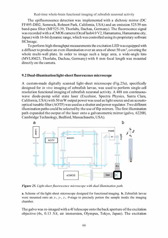
Real-time whole-brain functional imaging of zebrafish neuronal activity
66
The epifluorescence detection was implemented with a dichroic mirror (DC FF495-DI02, Semrock, Rohnert Park, California, USA) and an emission 525/39 nm band-pass filter (MF525-39, Thorlabs, Dachau, Germany). The fluorescence signal was recorded with a sCMOS camera (OrcaFlash4.0 V2, Hamamatsu, Hamamatsu city, Japan) with 16-bit dynamic range, which was controlled using its proprietary software HCImage.
To perform high-throughput measurements the excitation LED was equipped with a diffuser to produce an even illumination over an area of about 50 cm2, covering the whole multi-well plate. In order to image such a large area, a wide-angle lens (MVL8M23, Thorlabs, Dachau, Germany) with 8 mm focal length was mounted directly on the camera.
9.2 Dual-illumination light-sheet fluorescence microscope
A custom-made digitally scanned light-sheet microscope (Fig.25a), specifically designed for in vivo imaging of zebrafish larvae, was used to perform single-cell resolution functional imaging of zebrafish neuronal activity. A 488 nm continuous-wave diode-pump solid state laser (Excelsior, Spectra Physics, Santa Clara, California, USA) with 50 mW output power was used as light source and an acousto-optical tunable filter (AOTF) was used as a shutter and power regulator. Two different illumination paths could be selected by the use of flip mirrors. The first illumination path expanded the output of the laser onto a galvanometric mirror (galvo, 6220H, Cambridge Technology, Bedford, Massachusetts, USA).
Figure 25. Light-sheet fluorescence microscope with dual illumination path.
a. Scheme of the light-sheet microscope designed for functional imaging. b. Zebrafish larvae were mounted onto an x-, y-, z-, θ-stage to precisely potion the sample inside the imaging chamber.
The galvo was re-imaged with a 4f telescope onto the back aperture of the excitation objective (4x, 0.13 NA, air immersion, Olympus, Tokyo, Japan). The excitation
67
objective focused the illumination beam into the sample chamber and, by applying a sawtooth waveform to the galvo, the beam was rapidly scanned to form a virtual light sheet which coincided with the focal plane of a perpendicularly placed detection objective (20x, 1 NA, water immersion, Olympus, Tokyo, Japan). In the second illumination path a telescope adjusted the diameter of the Gaussian beam before the axicon (AX251-A, α = 1, Thorlabs, Dachau, Germany) to minimize the Gaussian contribution produced by the round tip. The self-reconstruction length of the resulting Bessel beam was then re-imaged with 3 additional lenses, each placed at 2f from each other, into the common Gaussian light path. A circular spatial filter was used close to a Fourier plane near the galvo to filter out any residual Gaussian contribution to the Bessel beam.
Figure 26. Dual-illumination light-sheet microscope characterization.
a. Measured point spread functions (PSFs) for the lateral and axial directions for Gaussian (grey) and Bessel illumination (blue) using sub-resolution fluorescent beads (100 nm diameter). Beads were automatically extracted and distilled into a PSF using commercial software (PSF distiller, Huygens Software, Scientific Volume Imaging BV, Hilversum, Netherlands). b. PSFs for Gaussian and Bessel illumination. c. Longitudinal beam profile. d. Transverse profile for the Gaussian (grey) and Bessel beam (blue). e. Table reporting the specifics of the setup in the two alternative illuminations. *theoretically derived values.
The capillary in which the sample was mounted (see below), was fixed on an x-, y-, z-, θ-stage (M-122.2DD and M-116.DG, Physik Instrumente, Karlsruhe, Germany), through a custom-made capillary holder (see Figure 28) and immersed in the sample chamber (Fig.25b). A heating system equipped with a thermocouple kept the sample chamber at the constant temperature of 28.5 °C during the whole measurement. Motorized stages allowed precise sample positioning and acquisition of z-stacks. Fluorescence was detected in a wide-field scheme with a tube lens forming an image onto the chip of a sCMOS camera (OrcaFlash4.0 V2, Hamamatsu, Hamamatsu city, Japan) having 16-bit of dynamic range.
66

Lapo Turrini
66
The epifluorescence detection was implemented with a dichroic mirror (DC FF495-DI02, Semrock, Rohnert Park, California, USA) and an emission 525/39 nm band-pass filter (MF525-39, Thorlabs, Dachau, Germany). The fluorescence signal was recorded with a sCMOS camera (OrcaFlash4.0 V2, Hamamatsu, Hamamatsu city, Japan) with 16-bit dynamic range, which was controlled using its proprietary software HCImage.
To perform high-throughput measurements the excitation LED was equipped with a diffuser to produce an even illumination over an area of about 50 cm2, covering the whole multi-well plate. In order to image such a large area, a wide-angle lens (MVL8M23, Thorlabs, Dachau, Germany) with 8 mm focal length was mounted directly on the camera.
9.2 Dual-illumination light-sheet fluorescence microscope
A custom-made digitally scanned light-sheet microscope (Fig.25a), specifically designed for in vivo imaging of zebrafish larvae, was used to perform single-cell resolution functional imaging of zebrafish neuronal activity. A 488 nm continuous-wave diode-pump solid state laser (Excelsior, Spectra Physics, Santa Clara, California, USA) with 50 mW output power was used as light source and an acousto-optical tunable filter (AOTF) was used as a shutter and power regulator. Two different illumination paths could be selected by the use of flip mirrors. The first illumination path expanded the output of the laser onto a galvanometric mirror (galvo, 6220H, Cambridge Technology, Bedford, Massachusetts, USA).
Figure 25. Light-sheet fluorescence microscope with dual illumination path.
a. Scheme of the light-sheet microscope designed for functional imaging. b. Zebrafish larvae were mounted onto an x-, y-, z-, θ-stage to precisely potion the sample inside the imaging chamber.
The galvo was re-imaged with a 4f telescope onto the back aperture of the excitation objective (4x, 0.13 NA, air immersion, Olympus, Tokyo, Japan). The excitation
67
objective focused the illumination beam into the sample chamber and, by applying a sawtooth waveform to the galvo, the beam was rapidly scanned to form a virtual light sheet which coincided with the focal plane of a perpendicularly placed detection objective (20x, 1 NA, water immersion, Olympus, Tokyo, Japan). In the second illumination path a telescope adjusted the diameter of the Gaussian beam before the axicon (AX251-A, α = 1, Thorlabs, Dachau, Germany) to minimize the Gaussian contribution produced by the round tip. The self-reconstruction length of the resulting Bessel beam was then re-imaged with 3 additional lenses, each placed at 2f from each other, into the common Gaussian light path. A circular spatial filter was used close to a Fourier plane near the galvo to filter out any residual Gaussian contribution to the Bessel beam.
Figure 26. Dual-illumination light-sheet microscope characterization.
a. Measured point spread functions (PSFs) for the lateral and axial directions for Gaussian (grey) and Bessel illumination (blue) using sub-resolution fluorescent beads (100 nm diameter). Beads were automatically extracted and distilled into a PSF using commercial software (PSF distiller, Huygens Software, Scientific Volume Imaging BV, Hilversum, Netherlands). b. PSFs for Gaussian and Bessel illumination. c. Longitudinal beam profile. d. Transverse profile for the Gaussian (grey) and Bessel beam (blue). e. Table reporting the specifics of the setup in the two alternative illuminations. *theoretically derived values.
The capillary in which the sample was mounted (see below), was fixed on an x-, y-, z-, θ-stage (M-122.2DD and M-116.DG, Physik Instrumente, Karlsruhe, Germany), through a custom-made capillary holder (see Figure 28) and immersed in the sample chamber (Fig.25b). A heating system equipped with a thermocouple kept the sample chamber at the constant temperature of 28.5 °C during the whole measurement. Motorized stages allowed precise sample positioning and acquisition of z-stacks. Fluorescence was detected in a wide-field scheme with a tube lens forming an image onto the chip of a sCMOS camera (OrcaFlash4.0 V2, Hamamatsu, Hamamatsu city, Japan) having 16-bit of dynamic range.
67

Real-time whole-brain functional imaging of zebrafish neuronal activity
68
A 525/39 nm filter (MF525-39, Thorlabs, Dachau, Germany) was used to bandpass filter the fluorescence emission and reject exctation light. The camera was operated in rolling shutter mode thereby creating a virtual confocal slit. With this configuration we obtained a system having the specifics showed in Figure 26.
The microscope was controlled via custom software written in LabVIEW 2012 (National Instruments, Austin, Texas, USA) using the Murmex library (Distrio, Amsterdam, Netherlands) in particular to synchronize the galvo movement with the camera rolling shutter pace.
9.3 Two-photon light-sheet microscope
A custom made two-photon light-sheet microscope was specially built to perform fast volumetric functional imaging of zebrafish neuronal activity (de Vito et al., 2020a, b, c). The setup (Fig.27) was equipped with a Chameleon Ultra II two-photon tuneable Ti:Sa laser (Coherent, Santa Clara, California, USA), with 140 fs pulse width and 80 MHz repetition rate, as an excitation source. The IR beam passed through an electro-optical modulator (LM0202, Qioptiq, Rhyl, Wales, UK) that alternately rotated its polarization; in this way a downstream polarizing beam-splitter was used to convey the laser beam into two excitation arms in order to perform double-sided illumination. A couple of galvanometric mirrors (6SD11015, Cambridge Technology, Bedford, Massachusetts, USA), a resonant and a closed loop one, generated the virtual light sheet and rapidly scanned it across the larva brain. Figure 27. Double-sided illumination two-photon light-sheet microscope.
Scheme of the two-photon light-sheet microscope specially designed to perform rapid whole brain imaging of the zebrafish larva neuronal activity. The IR femtosecond pulsed laser is rapidly scanned by a resonant galvanometric mirror, thus producing a virtual light sheet. The position of the sheet of light inside the brain of the larva is progressively moved by a slower closed loop galvo. To perform volumetric acquisition the detection objective is synchronously moved to adapt its focus to the plane that is time-by-time excited by the light sheet.
69
A couple of illumination objectives (4x, 0.4 NA, air immersion; Olympus, Tokyo, Japan), mounted on piezoelectric motors (PIFOC P-725, Physik Instrumente, Karlsruhe, Germany) for fine axial adjustments, focused two coplanar light sheets inside the sample chamber in order to cover the whole FOV. Double-sided illumination was necessary to obtain high photon density over a FOV large enough to image the entire encephalon of a zebrafish larva. The detection objective (20x, NA 1, water immersion; Olympus, Tokyo, Japan), placed at 90° with respect to the illumination axis, collected and projected the excited fluorescence to an sCMOS camera (OrcaFlash4.0 V3, Hamamatsu, Hamamatsu city, Japan). In order to perform fast volumetric imaging over the whole larva encephalon, the detection objective was mounted on a piezoelectric motor (identical to those mounted for the excitation objectives) that allowed fast displacement of the objective lens. To have sharp images of the same plane after each iteration of the objective, the piezo motor was synchronized with the closed loop galvo movement. Then, just before the camera chip a 10x objective (RMS10X, Plan Achromat, 0.25 NA, Olympus, Tokyo, Japan) operated a demagnification of the image to use a sub-array of the chip (512x512 px2) and thus speed up the acquisition. Indeed, directly choosing a lower magnification (lower NA) detection objective would have meant having the same spatial resolution but collecting much less fluorescence photons (as the photon collection efficiency scales like NA2). With the introduction of this demagnification step, we could combine low magnification without renouncing to the high NA of the detection objective. The final magnification of the system was 3x, reaching a pixel size of 2 µm, enough to sample neuronal nuclei (~ 5 µm) according to Nyquist-Shannon sampling theorem.
68

Lapo Turrini
68
A 525/39 nm filter (MF525-39, Thorlabs, Dachau, Germany) was used to bandpass filter the fluorescence emission and reject exctation light. The camera was operated in rolling shutter mode thereby creating a virtual confocal slit. With this configuration we obtained a system having the specifics showed in Figure 26.
The microscope was controlled via custom software written in LabVIEW 2012 (National Instruments, Austin, Texas, USA) using the Murmex library (Distrio, Amsterdam, Netherlands) in particular to synchronize the galvo movement with the camera rolling shutter pace.
9.3 Two-photon light-sheet microscope
A custom made two-photon light-sheet microscope was specially built to perform fast volumetric functional imaging of zebrafish neuronal activity (de Vito et al., 2020a, b, c). The setup (Fig.27) was equipped with a Chameleon Ultra II two-photon tuneable Ti:Sa laser (Coherent, Santa Clara, California, USA), with 140 fs pulse width and 80 MHz repetition rate, as an excitation source. The IR beam passed through an electro-optical modulator (LM0202, Qioptiq, Rhyl, Wales, UK) that alternately rotated its polarization; in this way a downstream polarizing beam-splitter was used to convey the laser beam into two excitation arms in order to perform double-sided illumination. A couple of galvanometric mirrors (6SD11015, Cambridge Technology, Bedford, Massachusetts, USA), a resonant and a closed loop one, generated the virtual light sheet and rapidly scanned it across the larva brain. Figure 27. Double-sided illumination two-photon light-sheet microscope.
Scheme of the two-photon light-sheet microscope specially designed to perform rapid whole brain imaging of the zebrafish larva neuronal activity. The IR femtosecond pulsed laser is rapidly scanned by a resonant galvanometric mirror, thus producing a virtual light sheet. The position of the sheet of light inside the brain of the larva is progressively moved by a slower closed loop galvo. To perform volumetric acquisition the detection objective is synchronously moved to adapt its focus to the plane that is time-by-time excited by the light sheet.
69
A couple of illumination objectives (4x, 0.4 NA, air immersion; Olympus, Tokyo, Japan), mounted on piezoelectric motors (PIFOC P-725, Physik Instrumente, Karlsruhe, Germany) for fine axial adjustments, focused two coplanar light sheets inside the sample chamber in order to cover the whole FOV. Double-sided illumination was necessary to obtain high photon density over a FOV large enough to image the entire encephalon of a zebrafish larva. The detection objective (20x, NA 1, water immersion; Olympus, Tokyo, Japan), placed at 90° with respect to the illumination axis, collected and projected the excited fluorescence to an sCMOS camera (OrcaFlash4.0 V3, Hamamatsu, Hamamatsu city, Japan). In order to perform fast volumetric imaging over the whole larva encephalon, the detection objective was mounted on a piezoelectric motor (identical to those mounted for the excitation objectives) that allowed fast displacement of the objective lens. To have sharp images of the same plane after each iteration of the objective, the piezo motor was synchronized with the closed loop galvo movement. Then, just before the camera chip a 10x objective (RMS10X, Plan Achromat, 0.25 NA, Olympus, Tokyo, Japan) operated a demagnification of the image to use a sub-array of the chip (512x512 px2) and thus speed up the acquisition. Indeed, directly choosing a lower magnification (lower NA) detection objective would have meant having the same spatial resolution but collecting much less fluorescence photons (as the photon collection efficiency scales like NA2). With the introduction of this demagnification step, we could combine low magnification without renouncing to the high NA of the detection objective. The final magnification of the system was 3x, reaching a pixel size of 2 µm, enough to sample neuronal nuclei (~ 5 µm) according to Nyquist-Shannon sampling theorem.
69

71
Chapter 10 Zebrafish husbandry
Zebrafish of the AB/Tübingen, albino, Tg(elavl3:GCaMP6s), and Tg(elavl3:H2B-GCaMP6s) strains were maintained according to standard procedures (Westerfield, 1993), in a 14 hour day - 10 hour night cycle at 28.5 °C, in a standalone aquarium system (Z-Hab Mini, Pentair, Apopka, Florida, USA). Zebrafish larvae of the Tg(elavl3:GCaMP6s) line used in wide-field fluorescence measurements were raised, from 24 hours post fertilization (hpf) onwards, in 0.003% (w/v) N-phenylthiourea (P7629, Sigma-Aldrich, Saint Louis, Missouri, USA) to inhibit melanogenesis and avoid the formation of skin pigments. Tg(elavl3:H2B-GCaMP6s) zebrafish line was brought on a heterozygous albino background; to obtain albino larvae used in the experiments, incross matings were performed between couples of heterozygous albino adults.
70

71
Chapter 10 Zebrafish husbandry
Zebrafish of the AB/Tübingen, albino, Tg(elavl3:GCaMP6s), and Tg(elavl3:H2B-GCaMP6s) strains were maintained according to standard procedures (Westerfield, 1993), in a 14 hour day - 10 hour night cycle at 28.5 °C, in a standalone aquarium system (Z-Hab Mini, Pentair, Apopka, Florida, USA). Zebrafish larvae of the Tg(elavl3:GCaMP6s) line used in wide-field fluorescence measurements were raised, from 24 hours post fertilization (hpf) onwards, in 0.003% (w/v) N-phenylthiourea (P7629, Sigma-Aldrich, Saint Louis, Missouri, USA) to inhibit melanogenesis and avoid the formation of skin pigments. Tg(elavl3:H2B-GCaMP6s) zebrafish line was brought on a heterozygous albino background; to obtain albino larvae used in the experiments, incross matings were performed between couples of heterozygous albino adults.
Lapo Turrini, Development of optical methods for real-time whole-brain functional imaging of zebrafish neuronal activity, © 2020 Author(s), content CC BY 4.0 International, metadata CC0 1.0 Universal, published by Firenze University Press (www.fupress.com), ISSN 2612-8020 (online), ISBN 978-88-5518-070-2 (PDF), DOI 10.36253/978-88-5518-070-2

73
Chapter 11 Sample mounting
Zebrafish larvae were mounted differently depending on the microscopy technique used to perform the measurements. All of the mounting procedures, however, had in common an embedding phase.
Each 3-4-5 dpf Tg(elavl3:GCaMP6s) and Tg(elavl3:H2B-GCaMP6s) larva was transferred into a reaction tube containing 1.5% (w/v) low melting temperature agarose (A9414, Sigma-Aldrich, Saint Louis, Missouri, USA) in fish water (150 mg/L Instant Ocean, 6.9 mg/L NaH2PO4, 12.5 mg/L Na2HPO4, pH 7.2), kept liquid at 38 °C. The larva was then taken up with a micropipette in a glass capillary (O.D. 1.5 mm, I.D. 0.86 mm, length 10 cm; B150-86-10, Sutter Instrument, Novato, California, USA). After gel polymerization, mounting proceeded as follow.
11.1 Wide-field fluorescence microscopy imaging
Mounting was performed under a stereomicroscope (Stemi 508, Carl Zeiss, Oberkochen, Germany). An agarose cylinder containing the larva was gently extruded from the capillary and laid on a microscope slide (1##02E, Menzel-Gläser, Thermo Scientific, Vantaa, Finland). In this phase, care was taken to orient the embedded larva with its dorsal portion facing upwards. A small drop of melted agarose was then placed on the rostral portion of the larva in order to immobilize the head in the precise orientation chosen. Next, the portion of agarose cylinder below the yolk was cut off with a scalpel and removed, thus freeing the tail of the larva. This procedure not only allowed measurements of tail movement but also improved the stability of encephalic imaging by preventing vibrations otherwise transmitted through the agarose cylinder. A flow chamber, allowing for solution exchange, was then assembled by attaching a coverslip to the microscope slide with double-sided tape (1.5 mm thick). In every experiment the chamber was initially filled with fish water. Sample remained in a natural horizontal position during the measurement.
11.2 Dual-illumination light-sheet fluorescence microscopy imaging
The agarose cylinder containing the larva was gently extruded until the head protruded from the glass. The glass capillary was then exposed to 2 mM d-tubocurarine (a paralyzing agent, 93750, Sigma-Aldrich, Saint Louis, Missouri, USA) in fish water
72

73
Chapter 11 Sample mounting
Zebrafish larvae were mounted differently depending on the microscopy technique used to perform the measurements. All of the mounting procedures, however, had in common an embedding phase.
Each 3-4-5 dpf Tg(elavl3:GCaMP6s) and Tg(elavl3:H2B-GCaMP6s) larva was transferred into a reaction tube containing 1.5% (w/v) low melting temperature agarose (A9414, Sigma-Aldrich, Saint Louis, Missouri, USA) in fish water (150 mg/L Instant Ocean, 6.9 mg/L NaH2PO4, 12.5 mg/L Na2HPO4, pH 7.2), kept liquid at 38 °C. The larva was then taken up with a micropipette in a glass capillary (O.D. 1.5 mm, I.D. 0.86 mm, length 10 cm; B150-86-10, Sutter Instrument, Novato, California, USA). After gel polymerization, mounting proceeded as follow.
11.1 Wide-field fluorescence microscopy imaging
Mounting was performed under a stereomicroscope (Stemi 508, Carl Zeiss, Oberkochen, Germany). An agarose cylinder containing the larva was gently extruded from the capillary and laid on a microscope slide (1##02E, Menzel-Gläser, Thermo Scientific, Vantaa, Finland). In this phase, care was taken to orient the embedded larva with its dorsal portion facing upwards. A small drop of melted agarose was then placed on the rostral portion of the larva in order to immobilize the head in the precise orientation chosen. Next, the portion of agarose cylinder below the yolk was cut off with a scalpel and removed, thus freeing the tail of the larva. This procedure not only allowed measurements of tail movement but also improved the stability of encephalic imaging by preventing vibrations otherwise transmitted through the agarose cylinder. A flow chamber, allowing for solution exchange, was then assembled by attaching a coverslip to the microscope slide with double-sided tape (1.5 mm thick). In every experiment the chamber was initially filled with fish water. Sample remained in a natural horizontal position during the measurement.
11.2 Dual-illumination light-sheet fluorescence microscopy imaging
The agarose cylinder containing the larva was gently extruded until the head protruded from the glass. The glass capillary was then exposed to 2 mM d-tubocurarine (a paralyzing agent, 93750, Sigma-Aldrich, Saint Louis, Missouri, USA) in fish water
Lapo Turrini, Development of optical methods for real-time whole-brain functional imaging of zebrafish neuronal activity, © 2020 Author(s), content CC BY 4.0 International, metadata CC0 1.0 Universal, published by Firenze University Press (www.fupress.com), ISSN 2612-8020 (online), ISBN 978-88-5518-070-2 (PDF), DOI 10.36253/978-88-5518-070-2

Real-time whole-brain functional imaging of zebrafish neuronal activity
74
for 10 minutes. Then, it was mounted into a custom-made capillary-holder (Fig.28) and fixed onto an x-, y-, z-, θ-stage (M-122.2DD and M-116.DG, Physik Instrumente, Karlsruhe, Germany) (Fig.25b). The capillary was immediately immersed into the sample chamber containing fish water kept at a constant temperature of 28.5 °C through a heating system. Due to the design of the setup, the sample stood in a head-down vertical orientation.
Figure 28. Capillary holder technical design.
The custom-made capillary holder consisted in a custom brass threaded cylinder having a through hole, screwed on a commercial grip head for universal capillary holder (cat. 5176210.003, Eppendorf, Hamburg, Germany). Capillary grip was ensured by an O-ring gasket system present inside the commercial grip head. The brass cylinder was made integral with the rotation motor through a set of three plastic screws. Dimensions in mm.
11.3 Two-photon light-sheet fluorescence microscopy imaging
Mounting was performed under a stereomicroscope (Stemi 508, Carl Zeiss, Oberkochen, Germany). The capillary containing the larva was first immersed in 2 mM d-tubocurarine in fish water for 10 minutes. Then, the agarose cylinder containing the embedded larva was gently extruded from the glass capillary and laid, with the dorsal portion facing upwards, on a modified microscope slide, consisting of a regular slide (1##02E, Menzel-Gläser, Thermo Scientific, Vantaa, Finland) at whose centre was glued with Canada balsam (C1795, Sigma-Aldrich, Saint Louis, Missouri, USA) a 7x3 mm piece of glass, 2 mm thick. The larva position was secured with a small drop of melted agarose. The peculiar slide used was necessary to position the larva at the appropriate height inside
Figure 29. Custom-made sample holder design.
A custom-made microscope slide was necessary for the light sheets not to be spoiled by the glass surface. Indeed, owing to the glass spacer introduced, the focused light-sheets (in red) could reach the larval zebrafish brain (in green) without intercepting the underlying microscope slide.
75
the sample chamber, without having glass deteriorating light-sheet quality (Fig.29). The modified microscope slide was then placed inside the imaging chamber
(Fig.30), which was immediately filled with fish water kept at 28.5 °C through a heating system. Sample stood in a natural horizontal position during the measurement.
Figure 30. Two-photon LSFM imaging chamber technical design.
The custom imaging chamber was designed to house conventional microscope slides (76x26x1 mm3) onto which immobilizing the zebrafish larva. The chamber, made of inert anticorodal aluminium alloy and anodized in black to minimize reflections, had 4 optical windows sealed with optical quality borosilicate coverslips (two bigger for entering with the light sheets, two smaller to allow visibility during sample positioning), open top to allow access of the water immersion detection objective, and bottom made of transparent polycarbonate to allow future virtual reality experiments. Distance between the two major optical windows was chosen ad hoc in order for the sheets of light to be focused in the centre of the chamber, producing the desired FOV. The imaging chamber was equipped with two cartridge heaters feedback-controlled by a thermocouple to keep temperature constant during measurements. Dimensions in mm.
74

Lapo Turrini
74
for 10 minutes. Then, it was mounted into a custom-made capillary-holder (Fig.28) and fixed onto an x-, y-, z-, θ-stage (M-122.2DD and M-116.DG, Physik Instrumente, Karlsruhe, Germany) (Fig.25b). The capillary was immediately immersed into the sample chamber containing fish water kept at a constant temperature of 28.5 °C through a heating system. Due to the design of the setup, the sample stood in a head-down vertical orientation.
Figure 28. Capillary holder technical design.
The custom-made capillary holder consisted in a custom brass threaded cylinder having a through hole, screwed on a commercial grip head for universal capillary holder (cat. 5176210.003, Eppendorf, Hamburg, Germany). Capillary grip was ensured by an O-ring gasket system present inside the commercial grip head. The brass cylinder was made integral with the rotation motor through a set of three plastic screws. Dimensions in mm.
11.3 Two-photon light-sheet fluorescence microscopy imaging
Mounting was performed under a stereomicroscope (Stemi 508, Carl Zeiss, Oberkochen, Germany). The capillary containing the larva was first immersed in 2 mM d-tubocurarine in fish water for 10 minutes. Then, the agarose cylinder containing the embedded larva was gently extruded from the glass capillary and laid, with the dorsal portion facing upwards, on a modified microscope slide, consisting of a regular slide (1##02E, Menzel-Gläser, Thermo Scientific, Vantaa, Finland) at whose centre was glued with Canada balsam (C1795, Sigma-Aldrich, Saint Louis, Missouri, USA) a 7x3 mm piece of glass, 2 mm thick. The larva position was secured with a small drop of melted agarose. The peculiar slide used was necessary to position the larva at the appropriate height inside
Figure 29. Custom-made sample holder design.
A custom-made microscope slide was necessary for the light sheets not to be spoiled by the glass surface. Indeed, owing to the glass spacer introduced, the focused light-sheets (in red) could reach the larval zebrafish brain (in green) without intercepting the underlying microscope slide.
75
the sample chamber, without having glass deteriorating light-sheet quality (Fig.29). The modified microscope slide was then placed inside the imaging chamber
(Fig.30), which was immediately filled with fish water kept at 28.5 °C through a heating system. Sample stood in a natural horizontal position during the measurement.
Figure 30. Two-photon LSFM imaging chamber technical design.
The custom imaging chamber was designed to house conventional microscope slides (76x26x1 mm3) onto which immobilizing the zebrafish larva. The chamber, made of inert anticorodal aluminium alloy and anodized in black to minimize reflections, had 4 optical windows sealed with optical quality borosilicate coverslips (two bigger for entering with the light sheets, two smaller to allow visibility during sample positioning), open top to allow access of the water immersion detection objective, and bottom made of transparent polycarbonate to allow future virtual reality experiments. Distance between the two major optical windows was chosen ad hoc in order for the sheets of light to be focused in the centre of the chamber, producing the desired FOV. The imaging chamber was equipped with two cartridge heaters feedback-controlled by a thermocouple to keep temperature constant during measurements. Dimensions in mm.
75

77
Chapter 12 Chemicals preparation
All stock solutions were prepared fresh the day of experiments. Stock solutions of pentylentetrazole (PTZ; P6500, Sigma-Aldrich, Saint Louis, Missouri, USA), valproic acid (VPA; P4543, Sigma-Aldrich, Saint Louis, Missouri, USA), tricaine (A5040, Sigma-Aldrich, Saint Louis, Missouri, USA), kynurenic acid (KYN; ab120256, Abcam, Cambridge, UK), tetrodotoxin (TTX; ab120055, Abcam, Cambridge, UK), and baclofen (BAC; ab120149, Abcam, Cambridge, UK) were prepared by dissolving powders in milliQ water (at 100 mM concentration for PTZ, VPA, and KYN; 4g/L for tricaine; 2 mM for TTX; 10 mM for BAC). The final concentrations used in the experiments were obtained by diluting each stock in fish water. D-tubocurarine (D-TC; 93750, Sigma-Aldrich, Saint Louis, Missouri, USA) was dissolved at 2 mM concentration directly in fish water.
76

77
Chapter 12 Chemicals preparation
All stock solutions were prepared fresh the day of experiments. Stock solutions of pentylentetrazole (PTZ; P6500, Sigma-Aldrich, Saint Louis, Missouri, USA), valproic acid (VPA; P4543, Sigma-Aldrich, Saint Louis, Missouri, USA), tricaine (A5040, Sigma-Aldrich, Saint Louis, Missouri, USA), kynurenic acid (KYN; ab120256, Abcam, Cambridge, UK), tetrodotoxin (TTX; ab120055, Abcam, Cambridge, UK), and baclofen (BAC; ab120149, Abcam, Cambridge, UK) were prepared by dissolving powders in milliQ water (at 100 mM concentration for PTZ, VPA, and KYN; 4g/L for tricaine; 2 mM for TTX; 10 mM for BAC). The final concentrations used in the experiments were obtained by diluting each stock in fish water. D-tubocurarine (D-TC; 93750, Sigma-Aldrich, Saint Louis, Missouri, USA) was dissolved at 2 mM concentration directly in fish water.
Lapo Turrini, Development of optical methods for real-time whole-brain functional imaging of zebrafish neuronal activity, © 2020 Author(s), content CC BY 4.0 International, metadata CC0 1.0 Universal, published by Firenze University Press (www.fupress.com), ISSN 2612-8020 (online), ISBN 978-88-5518-070-2 (PDF), DOI 10.36253/978-88-5518-070-2

79
Chapter 13 Optical measurements
13.1 Wide-field optical mapping measurements
Brain activity imaging was performed with the camera operating at 5 Hz (200 ms exposure time). Each measurement was composed of a 10-minute control recording, during which the larva was kept in fish water, followed by the addition of the drug solution at the desired concentration and subsequent recording for 30 to 120 minutes. When performing measurements of the whole larva to obtain data on tail movement along with GCaMP fluorescence, the camera was operated at 33 Hz with 5 ms exposure time (chosen to guarantee sharp images of the tail even during fast movements). Measurements were conducted at room temperature.
13.1.1 Combined electrographic and fluorescence recordings
Extracellular (local field potential, LFP) recordings were performed by inserting a borosilicate electrode, filled with 3 M NaCl, in the optical tectum of the larva. Electrical activity was recorded in current clamp mode with a Multiclamp 700B (Molecular Devices, Sunnyvale, California, USA). Analog signal was digitized at 10 kHz, low pass filtered at 1 kHz with a Digidata 1322A acquisition board, commanded with pClamp10 (Molecular Devices, Sunnyvale, California, USA). Simultaneous measurement of GCaMP6s fluorescence intensity was achieved with a fluorometric set up consisting of a blue LED excitation source and a photomultiplier tube (Cairn Research). Fluorescence collection area was adjusted manually to contain the entire encephalon of the larva. The photomultiplier signal was acquired and processed as described for electrode signal.
13.1.2 High-throughput measurements
To perform high-throughput measurements on freely moving larvae, we designed a black PVC multi-well plate composed of 61 cylindrical wells (diameter: 7 mm, depth: 5 mm, volume: ~200 µL) arranged in an hexagonal geometry to maximize the number of wells within a circular illumination spot (Fig.31). The material chosen to build the multi-well plate had the advantage of both being inert and offering a dark background for fluorescence measurements. Each 4 dpf Tg(elavl3:GCaMP6s) zebrafish larva was transferred into one of the 61 wells with an appropriate volume of fish water. After 20 min of habituation, 10 min of control recording were performed and then drug
78

79
Chapter 13 Optical measurements
13.1 Wide-field optical mapping measurements
Brain activity imaging was performed with the camera operating at 5 Hz (200 ms exposure time). Each measurement was composed of a 10-minute control recording, during which the larva was kept in fish water, followed by the addition of the drug solution at the desired concentration and subsequent recording for 30 to 120 minutes. When performing measurements of the whole larva to obtain data on tail movement along with GCaMP fluorescence, the camera was operated at 33 Hz with 5 ms exposure time (chosen to guarantee sharp images of the tail even during fast movements). Measurements were conducted at room temperature.
13.1.1 Combined electrographic and fluorescence recordings
Extracellular (local field potential, LFP) recordings were performed by inserting a borosilicate electrode, filled with 3 M NaCl, in the optical tectum of the larva. Electrical activity was recorded in current clamp mode with a Multiclamp 700B (Molecular Devices, Sunnyvale, California, USA). Analog signal was digitized at 10 kHz, low pass filtered at 1 kHz with a Digidata 1322A acquisition board, commanded with pClamp10 (Molecular Devices, Sunnyvale, California, USA). Simultaneous measurement of GCaMP6s fluorescence intensity was achieved with a fluorometric set up consisting of a blue LED excitation source and a photomultiplier tube (Cairn Research). Fluorescence collection area was adjusted manually to contain the entire encephalon of the larva. The photomultiplier signal was acquired and processed as described for electrode signal.
13.1.2 High-throughput measurements
To perform high-throughput measurements on freely moving larvae, we designed a black PVC multi-well plate composed of 61 cylindrical wells (diameter: 7 mm, depth: 5 mm, volume: ~200 µL) arranged in an hexagonal geometry to maximize the number of wells within a circular illumination spot (Fig.31). The material chosen to build the multi-well plate had the advantage of both being inert and offering a dark background for fluorescence measurements. Each 4 dpf Tg(elavl3:GCaMP6s) zebrafish larva was transferred into one of the 61 wells with an appropriate volume of fish water. After 20 min of habituation, 10 min of control recording were performed and then drug
Lapo Turrini, Development of optical methods for real-time whole-brain functional imaging of zebrafish neuronal activity, © 2020 Author(s), content CC BY 4.0 International, metadata CC0 1.0 Universal, published by Firenze University Press (www.fupress.com), ISSN 2612-8020 (online), ISBN 978-88-5518-070-2 (PDF), DOI 10.36253/978-88-5518-070-2

Real-time whole-brain functional imaging of zebrafish neuronal activity
80
stock solutions were added to each of the 61 wells to obtain the desired final concentration in 180 µL final total volume. Measurements were then run for 2 hours, a time sufficient for all the tested drugs to exert their action. High -throughput measurements were performed at room temperature, operating the camera at 5 Hz (200 ms exposure time).
Figure 31. High-throughput multi-well plate technical design.
A multi-well (61) plate was specifically designed to perform high-throughput measurements of larval movement and neuronal activity (GCaMP fluorescence). Wells had the same diameter (7 mm) of those in 96-wells plate, typically used for high-throughput behavioural drug screening assays in zebrafish. Dimensions in mm.
13.2 Dual-illumination light-sheet fluorescence microscopy measurements
For light-sheet microscopy functional imaging a line exposure time of 0.3 ms (corresponding to a virtual slit width of 201 µm) was used, resulting in a frame rate of 49 Hz, at a full resolution of 2048 px2. When using Bessel beam illumination, power was increased by a factor of three compared to Gaussian illumination. Typical laser power at the back focal plane of the excitation objective was 0.7 mW for Gaussian illumination and 2 mW for Bessel illumination. These power levels have been already reported in the literature to be safe in terms of photo-toxicity (Panier et al., 2013). Measurements were conducted at the constant temperature of 28.5 °C
In flickering quantification measurements, in order to assure that the evidenced changes in pixel brightness were not due to neuronal activity, 160 mg/L tricaine (A5040, Sigma-Aldrich, Saint Louis, Missouri, USA), a general anaesthetic that blocks voltage sensitive Na+ channels preferentially in neurons, was added to fish water. In measurements aiming at recording spontaneous neuronal activity, larvae were instead kept in fish water.
In measurements of 3D mapping of neuronal activity during the onset of drug-induced seizures, the sample chamber was filled with pentylentetrazole (PTZ) solution at the desired concentration in fish water. The larva was precisely positioned through the motor stages and after 15 minutes incubation in PTZ (an amount of time we saw to be sufficient for PTZ to exert its convulsive action) measurements were run. Starting from the dorsal surface of the larva we imaged sequentially, 4 minutes each, 24 planes of the larval encephalon 7 µm apart from each other, for an overall ~
81
160 µm thickness. Measurement depth was limited by the defined time-window of ~ 2 h during which D-TC exerted its reversible paralysing action.
13.3 Two-photon light-sheet fluorescence microscopy measurements
Before each two-photon light-sheet fluorescence microscopy recording, the laser was first aligned to have two coplanar light sheets covering the whole FOV, without overlap. Coarse alignment inside the imaging chamber was performed using a green fluorescent plastic rod (obtained from a fluorescent slide by Chroma Technology Corp, Bellows Falls, Vermont, USA) cut with approximately the same dimensions of a zebrafish larva (~ 1x1x3 mm3), glued on a custom microscope slide (identical to the one used for sample mounting, Fig.29). Fine alignment was then achieved directly on the larva, with the foresight to use very low power (0.3 W at the exit of the electro-optical modulator), not to expose the specimen to unnecessary electromagnetic radiation. Laser power during measurements was set to values ranging from 0.7 to 1 W (at the exit of the electro-optical modulator), depending on the fluorescence signal available. Imaging chamber was filled with fish water (~ 80 mL) and measurements were conducted at the constant temperature of 28.5 °C. Volumetric time-lapse recordings were performed moving the detection objective through a piezoelectric motor, accordingly to the plane illuminated by the light-sheets, reaching a volumetric framerate of 1 Hz, over 150-200 µm thickness. Typically, measurements in physiological conditions were run for 60 min. When recording aberrant neuronal activity, larvae were first imaged 5 minutes in control conditions before replacing a specific volume of fish water inside the imaging chamber with 100 mM PTZ stock solution, to obtain the final desired PTZ concentration. Seizure onset and propagation was recorded for 60 minutes.
80

Lapo Turrini
80
stock solutions were added to each of the 61 wells to obtain the desired final concentration in 180 µL final total volume. Measurements were then run for 2 hours, a time sufficient for all the tested drugs to exert their action. High -throughput measurements were performed at room temperature, operating the camera at 5 Hz (200 ms exposure time).
Figure 31. High-throughput multi-well plate technical design.
A multi-well (61) plate was specifically designed to perform high-throughput measurements of larval movement and neuronal activity (GCaMP fluorescence). Wells had the same diameter (7 mm) of those in 96-wells plate, typically used for high-throughput behavioural drug screening assays in zebrafish. Dimensions in mm.
13.2 Dual-illumination light-sheet fluorescence microscopy measurements
For light-sheet microscopy functional imaging a line exposure time of 0.3 ms (corresponding to a virtual slit width of 201 µm) was used, resulting in a frame rate of 49 Hz, at a full resolution of 2048 px2. When using Bessel beam illumination, power was increased by a factor of three compared to Gaussian illumination. Typical laser power at the back focal plane of the excitation objective was 0.7 mW for Gaussian illumination and 2 mW for Bessel illumination. These power levels have been already reported in the literature to be safe in terms of photo-toxicity (Panier et al., 2013). Measurements were conducted at the constant temperature of 28.5 °C
In flickering quantification measurements, in order to assure that the evidenced changes in pixel brightness were not due to neuronal activity, 160 mg/L tricaine (A5040, Sigma-Aldrich, Saint Louis, Missouri, USA), a general anaesthetic that blocks voltage sensitive Na+ channels preferentially in neurons, was added to fish water. In measurements aiming at recording spontaneous neuronal activity, larvae were instead kept in fish water.
In measurements of 3D mapping of neuronal activity during the onset of drug-induced seizures, the sample chamber was filled with pentylentetrazole (PTZ) solution at the desired concentration in fish water. The larva was precisely positioned through the motor stages and after 15 minutes incubation in PTZ (an amount of time we saw to be sufficient for PTZ to exert its convulsive action) measurements were run. Starting from the dorsal surface of the larva we imaged sequentially, 4 minutes each, 24 planes of the larval encephalon 7 µm apart from each other, for an overall ~
81
160 µm thickness. Measurement depth was limited by the defined time-window of ~ 2 h during which D-TC exerted its reversible paralysing action.
13.3 Two-photon light-sheet fluorescence microscopy measurements
Before each two-photon light-sheet fluorescence microscopy recording, the laser was first aligned to have two coplanar light sheets covering the whole FOV, without overlap. Coarse alignment inside the imaging chamber was performed using a green fluorescent plastic rod (obtained from a fluorescent slide by Chroma Technology Corp, Bellows Falls, Vermont, USA) cut with approximately the same dimensions of a zebrafish larva (~ 1x1x3 mm3), glued on a custom microscope slide (identical to the one used for sample mounting, Fig.29). Fine alignment was then achieved directly on the larva, with the foresight to use very low power (0.3 W at the exit of the electro-optical modulator), not to expose the specimen to unnecessary electromagnetic radiation. Laser power during measurements was set to values ranging from 0.7 to 1 W (at the exit of the electro-optical modulator), depending on the fluorescence signal available. Imaging chamber was filled with fish water (~ 80 mL) and measurements were conducted at the constant temperature of 28.5 °C. Volumetric time-lapse recordings were performed moving the detection objective through a piezoelectric motor, accordingly to the plane illuminated by the light-sheets, reaching a volumetric framerate of 1 Hz, over 150-200 µm thickness. Typically, measurements in physiological conditions were run for 60 min. When recording aberrant neuronal activity, larvae were first imaged 5 minutes in control conditions before replacing a specific volume of fish water inside the imaging chamber with 100 mM PTZ stock solution, to obtain the final desired PTZ concentration. Seizure onset and propagation was recorded for 60 minutes.
81

83
Chapter 14 Data analysis
14.1 Wide-field optical mapping measurements analysis
In each wide-field experiment, the GCaMP6s fluorescence signal from the whole larval encephalon or from different brain regions (telencephalon, optic tectum, cerebellum, medulla) was measured using ImageJ, by manually selecting the desired region of interest (ROI). The ROI’s mean fluorescence intensity for each time point was then calculated and, after background subtraction, the values obtained were further processed using a custom Matlab script to obtain the ΔF/F (Jia et al., 2011) signal as follows. The baseline for every time point ( ) was calculated (using Matlab function msbackadj with a running window and a step size of 2000 and 13333 points for 5 Hz and 33 Hz recordings, respectively) and subtracted from the fluorescence signal ( ), thus producing ΔF. These values were then normalized by dividing them by the baseline itself, obtaining ΔF/F .
Figure 32. Parabolic line selection for tail movement analysis.
The analysis of tail movement in head-restrained larvae was performed drawing a parabolic line selection, with its focus centred on the tail at rest, at a constant distance from the end of the yolk. Highlighted in colours the four main brain regions (in rostro-caudal direction, blue: telencephalon, orange: optic tectum, yellow: cerebellum, purple: medulla) used for activity analysis.
The traces shown in Figure 35b, c were processed differently, to highlight the dynamics of the basal brain activity in the experimental conditions shown. The mean fluorescence intensity of each 10 min control recording was calculated and used as in the ΔF/F calculation of each trace. In this way, the trace was not flattened by
82

83
Chapter 14 Data analysis
14.1 Wide-field optical mapping measurements analysis
In each wide-field experiment, the GCaMP6s fluorescence signal from the whole larval encephalon or from different brain regions (telencephalon, optic tectum, cerebellum, medulla) was measured using ImageJ, by manually selecting the desired region of interest (ROI). The ROI’s mean fluorescence intensity for each time point was then calculated and, after background subtraction, the values obtained were further processed using a custom Matlab script to obtain the ΔF/F (Jia et al., 2011) signal as follows. The baseline for every time point ( ) was calculated (using Matlab function msbackadj with a running window and a step size of 2000 and 13333 points for 5 Hz and 33 Hz recordings, respectively) and subtracted from the fluorescence signal ( ), thus producing ΔF. These values were then normalized by dividing them by the baseline itself, obtaining ΔF/F .
Figure 32. Parabolic line selection for tail movement analysis.
The analysis of tail movement in head-restrained larvae was performed drawing a parabolic line selection, with its focus centred on the tail at rest, at a constant distance from the end of the yolk. Highlighted in colours the four main brain regions (in rostro-caudal direction, blue: telencephalon, orange: optic tectum, yellow: cerebellum, purple: medulla) used for activity analysis.
The traces shown in Figure 35b, c were processed differently, to highlight the dynamics of the basal brain activity in the experimental conditions shown. The mean fluorescence intensity of each 10 min control recording was calculated and used as in the ΔF/F calculation of each trace. In this way, the trace was not flattened by
Lapo Turrini, Development of optical methods for real-time whole-brain functional imaging of zebrafish neuronal activity, © 2020 Author(s), content CC BY 4.0 International, metadata CC0 1.0 Universal, published by Firenze University Press (www.fupress.com), ISSN 2612-8020 (online), ISBN 978-88-5518-070-2 (PDF), DOI 10.36253/978-88-5518-070-2

Real-time whole-brain functional imaging of zebrafish neuronal activity
84
running baseline subtraction. Automatic peak detection was performed on ΔF/F traces using a custom Matlab script. The software first smoothed the traces by applying Savitzky-Golay filtering (sgolayfilt function, polynomial order: 7; frame length: 31 for 5 Hz acquisitions and 207 for 33 Hz acquisitions) then ran findpeaks function with 0.02 ΔF/F minimum peak prominence as a threshold, to measure the number of peaks in the trace along with their maximum ΔF/F value. Tail movement analysis was first performed with ImageJ using a parabolic line selection with its focus centred on the tail position at rest (Fig. 32). The intensity line profile of the selection was then measured in each frame and the coordinate of the maximum intensity point indicated the tail position at that time. Tail position values were then converted in mm. On tail movement traces peak analysis was also performed, by setting the minimum peak prominence to 0.05 mm and the minimum peak distance to 0.3 s, as a threshold. These parameters were chosen to optimize true motion detection above noise.
Correlation plots shown in Figure 40 were obtained by plotting against each other ΔF/F from two chosen regions. To distinguish fluorescence data occurring simultaneously with tail movement from those during rest, the tail position data were smoothed (running window of 150 points) and a threshold of 0.1 mm displacement of the tail was chosen to indicate significant movement. Cross-correlation analysis shown in Figure 41 was performed on brain recordings of larvae exposed to different PTZ concentrations, considering the four brain regions used for analysis and further dividing the data into the two hemispheres. For each condition considered, analysis was conducted on three progressive timeframes along a one-hour measurement. Correlation coefficients were calculated for any chosen pair of brain regions, averaged over three replicates and plotted in the cross-correlation matrix shown in the figure.
14.1.1 High-throughput measurements analysis
The fluorescence recordings from the high-throughput measurement (Fig.42) were analysed by selecting a region of interest (ROI) around each well and then running a custom ImageJ macro enabling parallel measurement of the maximum grey level detected in each ROI (after subtraction of the background measured in each ROI in a region of 230 px2 away from the larva). For larva tracking, the , coordinates of the centre of mass were extracted from the ROI after thresholding the image so to measure only pixels attributable to the larva. The routine ran these measurements on each frame of the acquired timelapse. Subsequently, intensity data were analysed to obtain ΔF/F traces as described above, while coordinates data were used to plot the larva trajectory and calculate its speed for each pair of frames.
14.2 Dual-illumination light-sheet fluorescence microscopy measurements analysis
14.2.1 Haemodynamic artefacts measurements analysis
The 16-bit depths images constituting each time-lapse were first converted from the proprietary Hamamatsu file format to tiff and simultaneously temporally down
85
sampled by a factor of 10 to save disc space resulting in an effective frame rate of ~5 Hz. In measurements performed to quantify flickering noise, larvae were treated with tricaine and no temporal downsampling was performed. GCaMP6s fluorescence signal was extracted with an ImageJ macro over circular ROIs manually selected around cell nuclei. The ΔF/F traces were obtained with a custom-written Matlab script as described before, after subtracting background measured over a ROI on the background proximal to the laser incoming direction.
The area affected by flickering (strong variations in baseline fluorescence intensity attributable to the upstream passage of blood cells into vessels) for Gaussian and Bessel beams illumination was estimated in a plane-wise manner by using a sequence of custom-made macros (ImageJ) and programs (LabVIEW). Using this automated method, 2D maps of severe flickering areas were obtained which allowed us to calculate the percentage of the entire encephalon prone to a substantial source of multiplicative noise.
Figure 33. Workflow to estimate area severely affected by flickering.
The first row refers to data obtained with Gaussian illumination while the second row was obtained with Bessel illumination. The raw data stack (a, f) was first temporally downsampled by calculating projections of the STD over 5 frames windows. Those STD stacks (b, g) were then treated over the entire image to further enhance the flickering areas, evidenced as bright horizontal stripes, using gamma, band-pass filter (BPF) and variance filter. The resulting time lapses (c, h) are projected along time dimension to create single STD images, which were adjusted to the same brightness scale before a common threshold was applied to binarize them (d, i). The binary images were then evaluated with a custom-written LabVIEW program to automatically localize the “blobs”. The bounding boxes (e, j) were used to calculate the overall area affected by flickering.
84

Lapo Turrini
84
running baseline subtraction. Automatic peak detection was performed on ΔF/F traces using a custom Matlab script. The software first smoothed the traces by applying Savitzky-Golay filtering (sgolayfilt function, polynomial order: 7; frame length: 31 for 5 Hz acquisitions and 207 for 33 Hz acquisitions) then ran findpeaks function with 0.02 ΔF/F minimum peak prominence as a threshold, to measure the number of peaks in the trace along with their maximum ΔF/F value. Tail movement analysis was first performed with ImageJ using a parabolic line selection with its focus centred on the tail position at rest (Fig. 32). The intensity line profile of the selection was then measured in each frame and the coordinate of the maximum intensity point indicated the tail position at that time. Tail position values were then converted in mm. On tail movement traces peak analysis was also performed, by setting the minimum peak prominence to 0.05 mm and the minimum peak distance to 0.3 s, as a threshold. These parameters were chosen to optimize true motion detection above noise.
Correlation plots shown in Figure 40 were obtained by plotting against each other ΔF/F from two chosen regions. To distinguish fluorescence data occurring simultaneously with tail movement from those during rest, the tail position data were smoothed (running window of 150 points) and a threshold of 0.1 mm displacement of the tail was chosen to indicate significant movement. Cross-correlation analysis shown in Figure 41 was performed on brain recordings of larvae exposed to different PTZ concentrations, considering the four brain regions used for analysis and further dividing the data into the two hemispheres. For each condition considered, analysis was conducted on three progressive timeframes along a one-hour measurement. Correlation coefficients were calculated for any chosen pair of brain regions, averaged over three replicates and plotted in the cross-correlation matrix shown in the figure.
14.1.1 High-throughput measurements analysis
The fluorescence recordings from the high-throughput measurement (Fig.42) were analysed by selecting a region of interest (ROI) around each well and then running a custom ImageJ macro enabling parallel measurement of the maximum grey level detected in each ROI (after subtraction of the background measured in each ROI in a region of 230 px2 away from the larva). For larva tracking, the , coordinates of the centre of mass were extracted from the ROI after thresholding the image so to measure only pixels attributable to the larva. The routine ran these measurements on each frame of the acquired timelapse. Subsequently, intensity data were analysed to obtain ΔF/F traces as described above, while coordinates data were used to plot the larva trajectory and calculate its speed for each pair of frames.
14.2 Dual-illumination light-sheet fluorescence microscopy measurements analysis
14.2.1 Haemodynamic artefacts measurements analysis
The 16-bit depths images constituting each time-lapse were first converted from the proprietary Hamamatsu file format to tiff and simultaneously temporally down
85
sampled by a factor of 10 to save disc space resulting in an effective frame rate of ~5 Hz. In measurements performed to quantify flickering noise, larvae were treated with tricaine and no temporal downsampling was performed. GCaMP6s fluorescence signal was extracted with an ImageJ macro over circular ROIs manually selected around cell nuclei. The ΔF/F traces were obtained with a custom-written Matlab script as described before, after subtracting background measured over a ROI on the background proximal to the laser incoming direction.
The area affected by flickering (strong variations in baseline fluorescence intensity attributable to the upstream passage of blood cells into vessels) for Gaussian and Bessel beams illumination was estimated in a plane-wise manner by using a sequence of custom-made macros (ImageJ) and programs (LabVIEW). Using this automated method, 2D maps of severe flickering areas were obtained which allowed us to calculate the percentage of the entire encephalon prone to a substantial source of multiplicative noise.
Figure 33. Workflow to estimate area severely affected by flickering.
The first row refers to data obtained with Gaussian illumination while the second row was obtained with Bessel illumination. The raw data stack (a, f) was first temporally downsampled by calculating projections of the STD over 5 frames windows. Those STD stacks (b, g) were then treated over the entire image to further enhance the flickering areas, evidenced as bright horizontal stripes, using gamma, band-pass filter (BPF) and variance filter. The resulting time lapses (c, h) are projected along time dimension to create single STD images, which were adjusted to the same brightness scale before a common threshold was applied to binarize them (d, i). The binary images were then evaluated with a custom-written LabVIEW program to automatically localize the “blobs”. The bounding boxes (e, j) were used to calculate the overall area affected by flickering.
85

Real-time whole-brain functional imaging of zebrafish neuronal activity
86
In details (Fig.33), both raw time-lapse recordings (Gauss and Bessel) were first processed with a custom-written ImageJ macro that calculated the standard deviation (STD) of 5 consecutive frames (window and step size 5 frames), to highlight the areas affected by the highest changes in fluorescence. The result was a pair of new time-lapse stacks composed by STD images (Fig.33b, g). After adjusting both time-lapses to the same brightness scale, they were processed by an additional ImageJ macro with the aim to enhance, in the images, the visibility of features having the highest STD values. The custom routine applied first a gamma correction of 1.1 (so as to enhance the visibility of brighter parts versus dim ones), second a bandpass filter (in order to filter out objects under a certain dimension) and third a variance filter (to highlight edges in the images) (Fig.33c,h). Each time-lapse was then collapsed to a single image using a z-projection of the STD. The resulting images were thresholded to a common value and converted to 8-bit binary where dark spots indicate the parts of the encephalon that had changed the most, in terms of fluorescence, during high frame rate (49 Hz) acquisition. The binary images (Fig.33d, i) where then analysed in a custom-written LabVIEW program that automatically found the bounding boxes of each identified particle. In the case of Gaussian illumination, the horizontal dimension of the bounding box of each particle was extended up to a mask corresponding to the free-hand selection of the encephalon of the larva. Indeed, due to Gaussian beam physical properties, when an obstacle stands on its path, the shadow produced is casted along the entire propagation length of the beam20.
In the case of the Bessel beam illumination, due to the self-healing properties of this kind of beam (see Bessel beams illumination) the bounding box was extended to a length corresponding to the theoretically calculated reconstruction length of the Bessel beam, which follows from simple trigonometric considerations:
𝑥𝑥 = 𝑡𝑡𝑡𝑡𝑡𝑡𝑡𝑡0.5 ∙ ℎ
where 𝑡𝑡 is the angle of the Bessel cone in the sample chamber, and ℎ is the height
of the bounding box. The LabVIEW program then automatically calculated the sum of all bounding boxes and their percentile of the free-hand selection of the entire encephalon. The characteristic horizontal stripes of the resulting areas confirmed that the method indicated shadowing artefacts and not individual neuronal activity.
For peak counting, the ΔF/F traces were loaded into a custom-written Matlab program and smoothed using the sgolayfilt function (polynomial order: 5; frame length: 7). The findpeaks function was then used to automatically detect peaks above the Gaussian and Bessel noise level, respectively, with a minimum peak prominence of 8.5% of ΔF/F . The correlation matrices were calculated using a custom-written Matlab program using the corr2 function. Noise (see Figure 47) was generated according to the following pseudo Matlab code to produce random noise that oscillates around an average of unity:
20 Only diffraction can mitigate the sharpness of the shadows produced, but the effects due to this phenomenon are visible only after long distances travelled.
87
𝑛𝑛𝑛𝑛𝑛𝑛𝑛𝑛𝑛𝑛 = 𝑆𝑆𝑆𝑆𝑆𝑆 .∗ 𝑟𝑟𝑎𝑎𝑛𝑛𝑎𝑎𝑛𝑛 + 1 The noise vector was than point-wise multiplied to the trace vector, which was
averaged to zero using:
𝑦𝑦 = (𝑡𝑡𝑟𝑟𝑎𝑎𝑡𝑡𝑛𝑛 − 𝜇𝜇) .∗ 𝑛𝑛𝑛𝑛𝑛𝑛𝑛𝑛𝑛𝑛
14.2.2 Bessel beam illumination light-sheet microscopy 3D optical mapping analysis
Measurements of 3D mapping during the onset of epileptic seizures were first converted from the proprietary Hamamatsu file format to tiff and simultaneously temporally down sampled by a factor of 10 (method: average), resulting in an effective frame rate of ~5 Hz, using a custom LabVIEW program. To further save disc space, tiff files were then 2x2 binned, (method: average) passing from 2048 px2 to 1024 px2, and converted in 8-bit depth images21, using ImageJ. This post-processing allowed for an 80x reduction in data weight without loss of information. Indeed, the temporal downsampling performed brought the actual framerate from the redundant 50 to 5 Hz, which represents a good sampling considering GCaMP kinetic. The binning procedure halved the linear lateral resolution without anyway compromising the optimal cellular resolution achieved. Moreover, both temporal downsampling and binning were perfomed using an averaging method, thus without wasting information. After background subtraction, the tiles of each temporal stack were registered using TurboReg function on ImageJ, in order to remove movement artefacts, and adjusted in rotation for display purpose if necessary.
In order to perform an automatic cell detection, from each pre-processed time-lapse stack an average intensity projection was produced (using ImageJ), which underwent a local contrast enhancement using CLAHE function. On each projection image a custom Matlab routine was then run, The_Cell_Detector.m, adapted from Kawashima et al. (Kawashima et al., 2016), which performed an automatic cell segmentation based on local contrast thresholding. The script saved as output a matrix containing the xy coordinates of the nucleus centre of all the detected cells, along with a spatial mask of detected cells distribution and an image showing colour cell tag overlaid to the projection (Fig.34) Then, to calculate ΔF/F traces for detected cells, each pre-processed time-lapse stack was loaded on Matlab using a custom script The_DF_F_Calculator.m, which used data saved by The_Cell_Detector.m routine to identify the pixels belonging to each cell and measure the average the ΔF/F trace for each cell The matrix containing the ΔF/F traces of all detected cells, saved as output of The_DF_F_Calculator.m, was then used in a third custom Matlab script The_Peaks_Finder.m.
This third routine, after applying sgolayfilt function (polynomial order: 3; frame length: 17) to smooth traces, performed an activity peak identification using findpeaks function (minimum peak prominence: 0.02). The script then summed, for each cell,
21 The dynamic range compression did not impair following fluorescence dynamics analysis.
86

Lapo Turrini
86
In details (Fig.33), both raw time-lapse recordings (Gauss and Bessel) were first processed with a custom-written ImageJ macro that calculated the standard deviation (STD) of 5 consecutive frames (window and step size 5 frames), to highlight the areas affected by the highest changes in fluorescence. The result was a pair of new time-lapse stacks composed by STD images (Fig.33b, g). After adjusting both time-lapses to the same brightness scale, they were processed by an additional ImageJ macro with the aim to enhance, in the images, the visibility of features having the highest STD values. The custom routine applied first a gamma correction of 1.1 (so as to enhance the visibility of brighter parts versus dim ones), second a bandpass filter (in order to filter out objects under a certain dimension) and third a variance filter (to highlight edges in the images) (Fig.33c,h). Each time-lapse was then collapsed to a single image using a z-projection of the STD. The resulting images were thresholded to a common value and converted to 8-bit binary where dark spots indicate the parts of the encephalon that had changed the most, in terms of fluorescence, during high frame rate (49 Hz) acquisition. The binary images (Fig.33d, i) where then analysed in a custom-written LabVIEW program that automatically found the bounding boxes of each identified particle. In the case of Gaussian illumination, the horizontal dimension of the bounding box of each particle was extended up to a mask corresponding to the free-hand selection of the encephalon of the larva. Indeed, due to Gaussian beam physical properties, when an obstacle stands on its path, the shadow produced is casted along the entire propagation length of the beam20.
In the case of the Bessel beam illumination, due to the self-healing properties of this kind of beam (see Bessel beams illumination) the bounding box was extended to a length corresponding to the theoretically calculated reconstruction length of the Bessel beam, which follows from simple trigonometric considerations:
𝑥𝑥 = 𝑡𝑡𝑡𝑡𝑡𝑡𝑡𝑡0.5 ∙ ℎ
where 𝑡𝑡 is the angle of the Bessel cone in the sample chamber, and ℎ is the height
of the bounding box. The LabVIEW program then automatically calculated the sum of all bounding boxes and their percentile of the free-hand selection of the entire encephalon. The characteristic horizontal stripes of the resulting areas confirmed that the method indicated shadowing artefacts and not individual neuronal activity.
For peak counting, the ΔF/F traces were loaded into a custom-written Matlab program and smoothed using the sgolayfilt function (polynomial order: 5; frame length: 7). The findpeaks function was then used to automatically detect peaks above the Gaussian and Bessel noise level, respectively, with a minimum peak prominence of 8.5% of ΔF/F . The correlation matrices were calculated using a custom-written Matlab program using the corr2 function. Noise (see Figure 47) was generated according to the following pseudo Matlab code to produce random noise that oscillates around an average of unity:
20 Only diffraction can mitigate the sharpness of the shadows produced, but the effects due to this phenomenon are visible only after long distances travelled.
87
𝑛𝑛𝑛𝑛𝑛𝑛𝑛𝑛𝑛𝑛 = 𝑆𝑆𝑆𝑆𝑆𝑆 .∗ 𝑟𝑟𝑎𝑎𝑛𝑛𝑎𝑎𝑛𝑛 + 1 The noise vector was than point-wise multiplied to the trace vector, which was
averaged to zero using:
𝑦𝑦 = (𝑡𝑡𝑟𝑟𝑎𝑎𝑡𝑡𝑛𝑛 − 𝜇𝜇) .∗ 𝑛𝑛𝑛𝑛𝑛𝑛𝑛𝑛𝑛𝑛
14.2.2 Bessel beam illumination light-sheet microscopy 3D optical mapping analysis
Measurements of 3D mapping during the onset of epileptic seizures were first converted from the proprietary Hamamatsu file format to tiff and simultaneously temporally down sampled by a factor of 10 (method: average), resulting in an effective frame rate of ~5 Hz, using a custom LabVIEW program. To further save disc space, tiff files were then 2x2 binned, (method: average) passing from 2048 px2 to 1024 px2, and converted in 8-bit depth images21, using ImageJ. This post-processing allowed for an 80x reduction in data weight without loss of information. Indeed, the temporal downsampling performed brought the actual framerate from the redundant 50 to 5 Hz, which represents a good sampling considering GCaMP kinetic. The binning procedure halved the linear lateral resolution without anyway compromising the optimal cellular resolution achieved. Moreover, both temporal downsampling and binning were perfomed using an averaging method, thus without wasting information. After background subtraction, the tiles of each temporal stack were registered using TurboReg function on ImageJ, in order to remove movement artefacts, and adjusted in rotation for display purpose if necessary.
In order to perform an automatic cell detection, from each pre-processed time-lapse stack an average intensity projection was produced (using ImageJ), which underwent a local contrast enhancement using CLAHE function. On each projection image a custom Matlab routine was then run, The_Cell_Detector.m, adapted from Kawashima et al. (Kawashima et al., 2016), which performed an automatic cell segmentation based on local contrast thresholding. The script saved as output a matrix containing the xy coordinates of the nucleus centre of all the detected cells, along with a spatial mask of detected cells distribution and an image showing colour cell tag overlaid to the projection (Fig.34) Then, to calculate ΔF/F traces for detected cells, each pre-processed time-lapse stack was loaded on Matlab using a custom script The_DF_F_Calculator.m, which used data saved by The_Cell_Detector.m routine to identify the pixels belonging to each cell and measure the average the ΔF/F trace for each cell The matrix containing the ΔF/F traces of all detected cells, saved as output of The_DF_F_Calculator.m, was then used in a third custom Matlab script The_Peaks_Finder.m.
This third routine, after applying sgolayfilt function (polynomial order: 3; frame length: 17) to smooth traces, performed an activity peak identification using findpeaks function (minimum peak prominence: 0.02). The script then summed, for each cell,
21 The dynamic range compression did not impair following fluorescence dynamics analysis.
87

Real-time whole-brain functional imaging of zebrafish neuronal activity
88
the prominence of all peaks detected above threshold, thus producing an integrated measurement of the overall activity of each cell over the recorded time. Finally, The_Peaks_Finder.m, using the spatial mask produced by The_Cell_Detector.m, attributed to each cell position a colour representing, in a colour-coded fashion, the sum of its peaks prominence, generating a tiff image, which was termed neuronal activity heatmap. All heatmap planes were then combined to reconstruct a stack, which represented the 3D neuronal activity map. See Appendix B for further details about the scripts.
Figure 34. Automatic neuron detection.
Single plane of a 4 dpf Tg(elavl3:H2B-GCaMP6s) zebrafish larva (left) and the result of automatic cell detection (right) operated with the custom Matlab script The_Cell_Detector.m (adapted from (Kawashima et al., 2016)). Based on local contrast thresholding, the script identified great part of neurons present in the imaged plane.
14.3 Two-photon light-sheet fluorescence microscopy whole-brain measurements analysis
Two-photon LSFM time-lapse stacks, composed by sequential volumetric acquisition of the larval brain, were first converted in hyperstacks using ImageJ. Each multidimensional hyperstack could be navigated both in z, choosing the desired depth inside the brain, and in time to see the temporal dynamics of a chosen plane. Five minutes temporal windows of the hyperstacks produced were processed through a
89
custom-made data-analysis pipeline written in Python language that performed the analysis in a pixel-wise fashion. In order to eliminate probable motion artefacts, the script first identified frames in which the larva moved with a displacement greater than one pixel and substituted them with an interpolation of the first flanking frames not affected by movement. After this step, the routine calculated the standard deviation (STD) over time of all the pixels composing the hyperstack. An arbitrary threshold was set on STD values, so as to produce a mask of all the pixels having STD greater than 10. Then, the Python script performed a temporal deconvolution of all the pixels of the hyperstack, using a modified version of the algorithm published by Friedrich et al. (Friedrich et al., 2017). After that, a correlation of all the pixels above threshold was performed. Results obtained were further processed through DBSCAN algorithm (Ester et al., 1996) to identify neuronal clusters based on correlation of activity. A cluster was defined any time a pixel had at least 300 pixels sharing with it a correlation Pearson’s r ≥ 0.9. Considering the final spatial resolution of our system, a single cell nucleus is described by ~ 3x3 pixels thus, the minimum 300 pixels necessary to identify a cluster correspond to ~ 33 cells. The script then calculated the average over time of the grey values of all the pixels composing each cluster. After that, a correlation of all pixels values (above and below threshold) with the average activity calculated for each cluster was performed. 3D maps of correlation were then produced by attributing a colour-code to statistically significant correlating (green) and anti-correlating (red) pixels. Each correlation map (one for each neuronal cluster isolated) represented a functional circuit composed by neurons functionally connected to one particular cluster, during the time-window of measurement.
88
Lapo Turrini
88
the prominence of all peaks detected above threshold, thus producing an integrated measurement of the overall activity of each cell over the recorded time. Finally, The_Peaks_Finder.m, using the spatial mask produced by The_Cell_Detector.m, attributed to each cell position a colour representing, in a colour-coded fashion, the sum of its peaks prominence, generating a tiff image, which was termed neuronal activity heatmap. All heatmap planes were then combined to reconstruct a stack, which represented the 3D neuronal activity map. See Appendix B for further details about the scripts.
Figure 34. Automatic neuron detection.
Single plane of a 4 dpf Tg(elavl3:H2B-GCaMP6s) zebrafish larva (left) and the result of automatic cell detection (right) operated with the custom Matlab script The_Cell_Detector.m (adapted from (Kawashima et al., 2016)). Based on local contrast thresholding, the script identified great part of neurons present in the imaged plane.
14.3 Two-photon light-sheet fluorescence microscopy whole-brain measurements analysis
Two-photon LSFM time-lapse stacks, composed by sequential volumetric acquisition of the larval brain, were first converted in hyperstacks using ImageJ. Each multidimensional hyperstack could be navigated both in z, choosing the desired depth inside the brain, and in time to see the temporal dynamics of a chosen plane. Five minutes temporal windows of the hyperstacks produced were processed through a
89
custom-made data-analysis pipeline written in Python language that performed the analysis in a pixel-wise fashion. In order to eliminate probable motion artefacts, the script first identified frames in which the larva moved with a displacement greater than one pixel and substituted them with an interpolation of the first flanking frames not affected by movement. After this step, the routine calculated the standard deviation (STD) over time of all the pixels composing the hyperstack. An arbitrary threshold was set on STD values, so as to produce a mask of all the pixels having STD greater than 10. Then, the Python script performed a temporal deconvolution of all the pixels of the hyperstack, using a modified version of the algorithm published by Friedrich et al. (Friedrich et al., 2017). After that, a correlation of all the pixels above threshold was performed. Results obtained were further processed through DBSCAN algorithm (Ester et al., 1996) to identify neuronal clusters based on correlation of activity. A cluster was defined any time a pixel had at least 300 pixels sharing with it a correlation Pearson’s r ≥ 0.9. Considering the final spatial resolution of our system, a single cell nucleus is described by ~ 3x3 pixels thus, the minimum 300 pixels necessary to identify a cluster correspond to ~ 33 cells. The script then calculated the average over time of the grey values of all the pixels composing each cluster. After that, a correlation of all pixels values (above and below threshold) with the average activity calculated for each cluster was performed. 3D maps of correlation were then produced by attributing a colour-code to statistically significant correlating (green) and anti-correlating (red) pixels. Each correlation map (one for each neuronal cluster isolated) represented a functional circuit composed by neurons functionally connected to one particular cluster, during the time-window of measurement.
89

91
Part III
Results
90

91
Part III
Results

93
Chapter 15 Optical mapping of zebrafish neuronal activity in a pharmacological model of epilepsy
15.1 GCaMP6s optical measurements show basal and PTZ-altered activity in the zebrafish brain
For this part of the work, we used a transgenic zebrafish line, generated during my Master thesis project, expressing in the cytoplasm of all CNS neurons the fast and sensitive calcium reporter GCaMP6s (Chen et al., 2013). Pan-neuronal expression in the Tg(elavl3:GCaMP6s) zebrafish encephalon provided a strong signal that maps throughout the whole larval brain, allowing us to clearly distinguish different anatomical areas of the encephalon such as the telencephalon, the optic tectum, the cerebellum and the medulla (Fig.35a). During wide-field fluorescence recording of brain activity, the larvae were mounted under the microscope in a setup allowing solution exchanges (see Sample mounting for details), so that each larva could be monitored in control conditions before adding the well-characterized convulsant agent PTZ at the desired concentration. This experimental protocol enabled the direct measurement of the onset of the compound activity as well as its steady effect at prolonged exposures.
Figure 35b shows a typical experiment in which 15 mM PTZ is added after 11 minutes of control recording. The ΔF/F trace (see Data analysis) clearly shows an increase of the baseline developing early after PTZ addition.
Compared to control, where few small peaks of spontaneous activity are visible (with a maximum amplitude of about 0.4), the effect of PTZ developed gradually over about ten minutes and then reached a steady convulsion activity with large and regularly paced calcium spikes. In the trace shown in Figure 35b, during the 50-60 minutes following the onset of PTZ effect, activity was regularly paced, with ΔF/F maximum amplitudes of 2-3. With more prolonged exposure to PTZ even larger bursts became evident (ΔF/F up to 5-6).
The data shown in Figure 35b demonstrate the high sensitivity of our recording method to the convulsant effects of PTZ. Moreover, these experiments demonstrate that different stages of convulsions can be recognized in the calcium trace, depending on both amplitude and frequency of the fluorescence peaks. It is also interesting to consider the signal baseline and its dynamics: due to projection of the fluorescence signal on one plane and the integration over the whole brain performed to obtain data such as those shown in Figure 35b, the measured baseline can indeed be interpreted as a measurement of basal brain activity of the larva. Our measurements are very
92
93
Chapter 15 Optical mapping of zebrafish neuronal activity in a pharmacological model of epilepsy
15.1 GCaMP6s optical measurements show basal and PTZ-altered activity in the zebrafish brain
For this part of the work, we used a transgenic zebrafish line, generated during my Master thesis project, expressing in the cytoplasm of all CNS neurons the fast and sensitive calcium reporter GCaMP6s (Chen et al., 2013). Pan-neuronal expression in the Tg(elavl3:GCaMP6s) zebrafish encephalon provided a strong signal that maps throughout the whole larval brain, allowing us to clearly distinguish different anatomical areas of the encephalon such as the telencephalon, the optic tectum, the cerebellum and the medulla (Fig.35a). During wide-field fluorescence recording of brain activity, the larvae were mounted under the microscope in a setup allowing solution exchanges (see Sample mounting for details), so that each larva could be monitored in control conditions before adding the well-characterized convulsant agent PTZ at the desired concentration. This experimental protocol enabled the direct measurement of the onset of the compound activity as well as its steady effect at prolonged exposures.
Figure 35b shows a typical experiment in which 15 mM PTZ is added after 11 minutes of control recording. The ΔF/F trace (see Data analysis) clearly shows an increase of the baseline developing early after PTZ addition.
Compared to control, where few small peaks of spontaneous activity are visible (with a maximum amplitude of about 0.4), the effect of PTZ developed gradually over about ten minutes and then reached a steady convulsion activity with large and regularly paced calcium spikes. In the trace shown in Figure 35b, during the 50-60 minutes following the onset of PTZ effect, activity was regularly paced, with ΔF/F maximum amplitudes of 2-3. With more prolonged exposure to PTZ even larger bursts became evident (ΔF/F up to 5-6).
The data shown in Figure 35b demonstrate the high sensitivity of our recording method to the convulsant effects of PTZ. Moreover, these experiments demonstrate that different stages of convulsions can be recognized in the calcium trace, depending on both amplitude and frequency of the fluorescence peaks. It is also interesting to consider the signal baseline and its dynamics: due to projection of the fluorescence signal on one plane and the integration over the whole brain performed to obtain data such as those shown in Figure 35b, the measured baseline can indeed be interpreted as a measurement of basal brain activity of the larva. Our measurements are very
Lapo Turrini, Development of optical methods for real-time whole-brain functional imaging of zebrafish neuronal activity, © 2020 Author(s), content CC BY 4.0 International, metadata CC0 1.0 Universal, published by Firenze University Press (www.fupress.com), ISSN 2612-8020 (online), ISBN 978-88-5518-070-2 (PDF), DOI 10.36253/978-88-5518-070-2
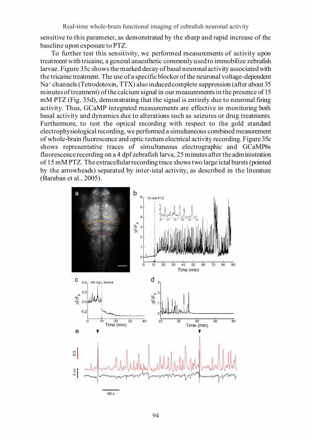
Real-time whole-brain functional imaging of zebrafish neuronal activity
94
sensitive to this parameter, as demonstrated by the sharp and rapid increase of the baseline upon exposure to PTZ.
To further test this sensitivity, we performed measurements of activity upon treatment with tricaine, a general anaesthetic commonly used to immobilize zebrafish larvae. Figure 35c shows the marked decay of basal neuronal activity associated with the tricaine treatment. The use of a specific blocker of the neuronal voltage-dependent Na+ channels (Tetrodotoxin, TTX) also induced complete suppression (after about 35 minutes of treatment) of the calcium signal in our measurements in the presence of 15 mM PTZ (Fig. 35d), demonstrating that the signal is entirely due to neuronal firing activity. Thus, GCaMP integrated measurements are effective in monitoring both basal activity and dynamics due to alterations such as seizures or drug treatments. Furthermore, to test the optical recording with respect to the gold standard electrophysiological recording, we performed a simultaneous combined measurement of whole-brain fluorescence and optic tectum electrical activity recording. Figure 35e shows representative traces of simultaneous electrographic and GCaMP6s fluorescence recording on a 4 dpf zebrafish larva, 25 minutes after the adm inistration of 15 mM PTZ. The extracellular recording trace shows two large ictal bursts (pointed by the arrowheads) separated by inter-ictal activity, as described in the literature (Baraban et al., 2005).
95
Figure 35. Brain activity recording with GCaMP6s.
a. Wide-field fluorescence image of the encephalon of a 4 dpf larva expressing GCaMP6s under elavl3 promoter. The four main zebrafish brain regions used for further analysis are highlighted (in rostro-caudal order: Telencephalon, blue; Optic tectum, orange; Cerebellum, yellow; Medulla, purple). Scale bar: 100 µm. b. Time trace of fluorescence (ΔF/F , see Data analysis for details) in control conditions and after addition of 15 mM PTZ. Fluorescence data are integrated over the whole brain of the larva and sampled at 5 Hz. The inset shows a shorter time interval of the trace to better display Ca2+ peak shape and regularity. c. ΔF/F trace of an experiment in which tricaine (160 mg/L) was added at the time indicated and subsequent decay of neuronal activity was monitored. The ΔF/F values become negative after tricaine administration since reference level was measured in control conditions (see Data analysis for details). d. ΔF/F trace showing sharp brain activity decay in a larva simultaneously treated with 15 mM PTZ and 5 µM TTX. After approximately 35 minutes upon drugs administration, TTX action completely suppressed neuronal seizure activity induced by PTZ. e. Representative trace of simultaneous electrographic (black trace) and GCaMP6s fluorescence (red trace) recording on a 4 dpf zebrafish larva with head restrained in 1.5% low gelling temperature agarose and free tail (as described in Optical measurements). The recording was taken 25 minutes after administration of 15 mM PTZ. Comparison of the two traces demonstrates the excellent correspondence between the two measurement methods.
15.2 GCaMP6s fluorescence measurements are sensitive to different PTZ concentrations
We next characterized the response of zebrafish larvae to different PTZ concentrations. Figure 36a shows GCaMP6s recordings in 0 (control), 1, 2.5, 7.5 and 15 mM PTZ. The figure shows a clear dependence of both peak amplitudes and frequencies on PTZ concentration: at 1 and 2.5 mM PTZ, the peaks amplitudes are only slightly larger than control; on the other hand, at 7.5 and 15 mM PTZ we observed a marked increase in amplitude of the spikes and the appearance of regularly paced patterns of activity.
Particularly at 15 mM PTZ the ΔF/F signal displayed long (about 5 minutes) and very large (ΔF/F up to 4-5) increases consisting of clusters of closely spaced spikes (Fig.36a, inset).
Each burst is followed by a period of low activity before a new burst appears. We observed some variability in the latency for appearance of these characteristic convulsive clusters of seizures (as visible from a comparison between Figure 35b and the trace at 15 mM in Figure 36a), but the periodicity of the convulsive and rest periods was remarkably reproducible across larvae.
Observation of the data in Figure 36a shows that GCaMP measurements are sensitive to a range of activity alterations as induced by different PTZ concentrations. Our recordings enabled quantitative analysis of calcium activity in terms of both amplitude and frequency. Based on automated data analysis (see Data analysis) we identified each peak and measured its amplitude and the frequency of firing in the recordings. Figure 36b, c show the average peak amplitudes and frequencies measured at different PTZ concentrations in the range between 0 and 15 mM. The ΔF/F peak fluorescence (Fig.36b) exhibits a linear dependence on PTZ concentration (R =
94

Lapo Turrini
94
sensitive to this parameter, as demonstrated by the sharp and rapid increase of the baseline upon exposure to PTZ.
To further test this sensitivity, we performed measurements of activity upon treatment with tricaine, a general anaesthetic commonly used to immobilize zebrafish larvae. Figure 35c shows the marked decay of basal neuronal activity associated with the tricaine treatment. The use of a specific blocker of the neuronal voltage-dependent Na+ channels (Tetrodotoxin, TTX) also induced complete suppression (after about 35 minutes of treatment) of the calcium signal in our measurements in the presence of 15 mM PTZ (Fig. 35d), demonstrating that the signal is entirely due to neuronal firing activity. Thus, GCaMP integrated measurements are effective in monitoring both basal activity and dynamics due to alterations such as seizures or drug treatments. Furthermore, to test the optical recording with respect to the gold standard electrophysiological recording, we performed a simultaneous combined measurement of whole-brain fluorescence and optic tectum electrical activity recording. Figure 35e shows representative traces of simultaneous electrographic and GCaMP6s fluorescence recording on a 4 dpf zebrafish larva, 25 minutes after the adm inistration of 15 mM PTZ. The extracellular recording trace shows two large ictal bursts (pointed by the arrowheads) separated by inter-ictal activity, as described in the literature (Baraban et al., 2005).
95
Figure 35. Brain activity recording with GCaMP6s.
a. Wide-field fluorescence image of the encephalon of a 4 dpf larva expressing GCaMP6s under elavl3 promoter. The four main zebrafish brain regions used for further analysis are highlighted (in rostro-caudal order: Telencephalon, blue; Optic tectum, orange; Cerebellum, yellow; Medulla, purple). Scale bar: 100 µm. b. Time trace of fluorescence (ΔF/F , see Data analysis for details) in control conditions and after addition of 15 mM PTZ. Fluorescence data are integrated over the whole brain of the larva and sampled at 5 Hz. The inset shows a shorter time interval of the trace to better display Ca2+ peak shape and regularity. c. ΔF/F trace of an experiment in which tricaine (160 mg/L) was added at the time indicated and subsequent decay of neuronal activity was monitored. The ΔF/F values become negative after tricaine administration since reference level was measured in control conditions (see Data analysis for details). d. ΔF/F trace showing sharp brain activity decay in a larva simultaneously treated with 15 mM PTZ and 5 µM TTX. After approximately 35 minutes upon drugs administration, TTX action completely suppressed neuronal seizure activity induced by PTZ. e. Representative trace of simultaneous electrographic (black trace) and GCaMP6s fluorescence (red trace) recording on a 4 dpf zebrafish larva with head restrained in 1.5% low gelling temperature agarose and free tail (as described in Optical measurements). The recording was taken 25 minutes after administration of 15 mM PTZ. Comparison of the two traces demonstrates the excellent correspondence between the two measurement methods.
15.2 GCaMP6s fluorescence measurements are sensitive to different PTZ concentrations
We next characterized the response of zebrafish larvae to different PTZ concentrations. Figure 36a shows GCaMP6s recordings in 0 (control), 1, 2.5, 7.5 and 15 mM PTZ. The figure shows a clear dependence of both peak amplitudes and frequencies on PTZ concentration: at 1 and 2.5 mM PTZ, the peaks amplitudes are only slightly larger than control; on the other hand, at 7.5 and 15 mM PTZ we observed a marked increase in amplitude of the spikes and the appearance of regularly paced patterns of activity.
Particularly at 15 mM PTZ the ΔF/F signal displayed long (about 5 minutes) and very large (ΔF/F up to 4-5) increases consisting of clusters of closely spaced spikes (Fig.36a, inset).
Each burst is followed by a period of low activity before a new burst appears. We observed some variability in the latency for appearance of these characteristic convulsive clusters of seizures (as visible from a comparison between Figure 35b and the trace at 15 mM in Figure 36a), but the periodicity of the convulsive and rest periods was remarkably reproducible across larvae.
Observation of the data in Figure 36a shows that GCaMP measurements are sensitive to a range of activity alterations as induced by different PTZ concentrations. Our recordings enabled quantitative analysis of calcium activity in terms of both amplitude and frequency. Based on automated data analysis (see Data analysis) we identified each peak and measured its amplitude and the frequency of firing in the recordings. Figure 36b, c show the average peak amplitudes and frequencies measured at different PTZ concentrations in the range between 0 and 15 mM. The ΔF/F peak fluorescence (Fig.36b) exhibits a linear dependence on PTZ concentration (R =
95

Real-time whole-brain functional imaging of zebrafish neuronal activity
96
0.992). Firing rates (Fig.36c), on the other hand, do increase with PTZ concentration but in a nonlinear manner. In the figures, measurements are also reported for larvae that had been pre-incubated with the anti-convulsant agent valproic acid (VPA, 5 mM) for one hour before the treatment with PTZ (at 15 mM). The data clearly show that the anti-epileptic effect of this drug (one of the most commonly used in the treatment of epilepsy in humans) was revealed extremely well by our method, since the ΔF/F peak amplitude and frequencies measured upon treatment with this drug were not distinguishable from the control levels. The linear response observed for the ΔF/F signal over the range of PTZ concentrations explored is interesting in the frame of studying mutations, which have been associated with epilepsy but may not lead by themselves to evident behavioural phenotypes.
Using PTZ as a standard in the field, we assessed the simplest and most robust method to quantify the effects of this compound on larval brain activity. For application of GCaMP6s activity measurements in a high-throughput drug screening assay (see below) we tested whether a simple time-averaged fluorescence over the whole recording in a given condition would be effective in detecting alterations of brain activity in a concentration-dependent manner. The data are shown in Appendix Figure A1 and demonstrate that this simpler method is applicable to an analysis requiring less detail but faster processing such as demanded in high -throughput assays.
97
Figure 36. Effects of different PTZ concentrations on brain activity.
a. ΔF/F is plotted as a function of time for control conditions and increasing PTZ concentrations as indicated. Upper left panels show images acquired at the points indicated during the recording at 15 mM PTZ, demonstrating the large dynamic range of the signal and lack of saturation even at the highest recorded levels. The inset on the upper right shows a single cluster of closely spaced Ca2+ spikes occurring at 15 mM PTZ and displayed on a magnified time scale. ΔF/F scale bar: 100%. b. Average amplitude of peaks detected over one hour registration for each larva recorded (see Data analysis for details about automatic peak detection). The red symbol represents measurements performed on larvae treated with 15 mM PTZ after a pre-incubation of one hour in 5 mM valproic acid (VPA). The linear regression through the PTZ-only measurements (blue dashed line) produces a slope of 0.037/mM, Pearsons’s r = 0.992. N = 6 (0 mM), 7 (1 mM), 5 (2.5 mM), 6 (7.5 mM), 7 (15 mM), 3 (15 mM + 5 mM VPA). Error is SEM and were not visible is smaller than symbol size. c. Average peak frequency as a function of PTZ concentration. N is the same as in panel b.
15.3 Correlation analysis among brain regions and locomotor activity
One of the main advantages of optical imaging with respect to the use of an electrode is the capability of simultaneously monitoring activity in different brain regions. Furthermore, with the very large field of view of our microscope we could image the whole larva, thus conducting simultaneous measurements of brain activity and tail movement in head restrained larvae (the tail was free to move due to the method adopted for mounting the larva on the slide, as described in Sample mounting). Imaging of the tail and its movements was facilitated by the fluorescence signal from GCaMP6s expressed in CNS neurons of the spinal cord. We analysed fluorescence dynamics in four distinct brain regions: telencephalon, optic tectum, cerebellum and medulla (as evidenced by the coloured profiles in Figure 35a). Figure 37 shows typical results obtained for the recording of brain activity and tail movement at 0, 1 and 15 mM PTZ concentration. The general patterns of activity and peak amplitudes reflect the results shown in Figure 36 for the signal averaged over the whole brain. Distinguishing the different brain regions, however, allows some interesting observations. During spontaneous activity (CTRL, Fig.37a) we noticed that the activities in the optic tectum, cerebellum and medulla were well correlated, while the telencephalon exhibits independent patterns. Moreover, while the larger peaks in the three caudal regions of the brain correlated with large movements of the tail, telencephalon activity was not always linked with large movements. Figure 37d shows an enlarged part of the fluorescence and tail movement traces, demonstrating that in this condition most of the tail movements are brief, small amplitude beats consisting of a single small tail swing.
These movements (also shown in Figure 37g) can be classified as “beat and glide” movements (Kalueff et al., 2013), and are not paired with measurable changes of fluorescence (most likely due to the loss of sensitivity caused by integrating the signal over large encephalic areas in wide field imaging). Compared to control, at 1 mM PTZ (Fig.37b) we observed that telencephalon correlation with the caudal regions increased, even though some instances of independent peaks persisted. As shown also by the data in Figure 36, at this PTZ concentration, we observed the appearance of
96

Lapo Turrini
96
0.992). Firing rates (Fig.36c), on the other hand, do increase with PTZ concentration but in a nonlinear manner. In the figures, measurements are also reported for larvae that had been pre-incubated with the anti-convulsant agent valproic acid (VPA, 5 mM) for one hour before the treatment with PTZ (at 15 mM). The data clearly show that the anti-epileptic effect of this drug (one of the most commonly used in the treatment of epilepsy in humans) was revealed extremely well by our method, since the ΔF/F peak amplitude and frequencies measured upon treatment with this drug were not distinguishable from the control levels. The linear response observed for the ΔF/F signal over the range of PTZ concentrations explored is interesting in the frame of studying mutations, which have been associated with epilepsy but may not lead by themselves to evident behavioural phenotypes.
Using PTZ as a standard in the field, we assessed the simplest and most robust method to quantify the effects of this compound on larval brain activity. For application of GCaMP6s activity measurements in a high-throughput drug screening assay (see below) we tested whether a simple time-averaged fluorescence over the whole recording in a given condition would be effective in detecting alterations of brain activity in a concentration-dependent manner. The data are shown in Appendix Figure A1 and demonstrate that this simpler method is applicable to an analysis requiring less detail but faster processing such as demanded in high -throughput assays.
97
Figure 36. Effects of different PTZ concentrations on brain activity.
a. ΔF/F is plotted as a function of time for control conditions and increasing PTZ concentrations as indicated. Upper left panels show images acquired at the points indicated during the recording at 15 mM PTZ, demonstrating the large dynamic range of the signal and lack of saturation even at the highest recorded levels. The inset on the upper right shows a single cluster of closely spaced Ca2+ spikes occurring at 15 mM PTZ and displayed on a magnified time scale. ΔF/F scale bar: 100%. b. Average amplitude of peaks detected over one hour registration for each larva recorded (see Data analysis for details about automatic peak detection). The red symbol represents measurements performed on larvae treated with 15 mM PTZ after a pre-incubation of one hour in 5 mM valproic acid (VPA). The linear regression through the PTZ-only measurements (blue dashed line) produces a slope of 0.037/mM, Pearsons’s r = 0.992. N = 6 (0 mM), 7 (1 mM), 5 (2.5 mM), 6 (7.5 mM), 7 (15 mM), 3 (15 mM + 5 mM VPA). Error is SEM and were not visible is smaller than symbol size. c. Average peak frequency as a function of PTZ concentration. N is the same as in panel b.
15.3 Correlation analysis among brain regions and locomotor activity
One of the main advantages of optical imaging with respect to the use of an electrode is the capability of simultaneously monitoring activity in different brain regions. Furthermore, with the very large field of view of our microscope we could image the whole larva, thus conducting simultaneous measurements of brain activity and tail movement in head restrained larvae (the tail was free to move due to the method adopted for mounting the larva on the slide, as described in Sample mounting). Imaging of the tail and its movements was facilitated by the fluorescence signal from GCaMP6s expressed in CNS neurons of the spinal cord. We analysed fluorescence dynamics in four distinct brain regions: telencephalon, optic tectum, cerebellum and medulla (as evidenced by the coloured profiles in Figure 35a). Figure 37 shows typical results obtained for the recording of brain activity and tail movement at 0, 1 and 15 mM PTZ concentration. The general patterns of activity and peak amplitudes reflect the results shown in Figure 36 for the signal averaged over the whole brain. Distinguishing the different brain regions, however, allows some interesting observations. During spontaneous activity (CTRL, Fig.37a) we noticed that the activities in the optic tectum, cerebellum and medulla were well correlated, while the telencephalon exhibits independent patterns. Moreover, while the larger peaks in the three caudal regions of the brain correlated with large movements of the tail, telencephalon activity was not always linked with large movements. Figure 37d shows an enlarged part of the fluorescence and tail movement traces, demonstrating that in this condition most of the tail movements are brief, small amplitude beats consisting of a single small tail swing.
These movements (also shown in Figure 37g) can be classified as “beat and glide” movements (Kalueff et al., 2013), and are not paired with measurable changes of fluorescence (most likely due to the loss of sensitivity caused by integrating the signal over large encephalic areas in wide field imaging). Compared to control, at 1 mM PTZ (Fig.37b) we observed that telencephalon correlation with the caudal regions increased, even though some instances of independent peaks persisted. As shown also by the data in Figure 36, at this PTZ concentration, we observed the appearance of
97

Real-time whole-brain functional imaging of zebrafish neuronal activity
98
some peaks with a larger amplitude than control peaks (the dotted line indicates the maximum value of ΔF/F typically reached in control recordings). These peaks can, therefore, be attributed to the alterations induced by PTZ. It is interesting to notice that, some of these peaks were associated with large tail movements (that would be conducive to swimming, if the larva were free to swim), but many others (highlighted by arrowheads in the figure) were not associated with any tail movement or, at most, with very small tail deflections that would not produce detectable movements in behavioural assays. Indeed, we noticed that additionally to the infrequent but large tail swings (Fig.37b, h), at 1 mM PTZ concentration, the larva exhibited frequent small tail movements associated with detectable changes in the ΔF/F signal (Fig.37e). We noticed that, compared to control movements, these are more clustered and exhibit a larger number of tail beats per event. These movements can thus be classified as “dart” movements (Kalueff et al., 2013). At 15 mM PTZ (Fig.37c) we observed the complete synchronicity of activity in the four brain regions, the appearance of very large, regularly paced peaks of activity which are associated with larger tail movements, i.e. with the stage III (Baraban et al., 2005) convulsive swimming detected also in behavioural assays. We also noticed a correlation between peak intensity and the amplitude of tail movement, with higher peaks being associated with powerful swimming bouts (Fig.37c, f, i) and lower peaks with smaller tail fluctuations. Despite vigorous tail movements, the agarose-embedded head of the larva remained very stable during the measurements, thus avoiding potential movement artefacts (see Sample mounting for more details). The stability of the sample enabled measurements in the absence of paralyzing agents, with the advantage of allowing combined fluorescence and tail movement measurements such as those shown in Figure 37.
99
Figure 37. Simultaneous measurement of brain activity and tail movement.
a. Time trace of tail movement (black line) and fluorescence (ΔF/F ) analysed in control conditions (0 mM PTZ) for four brain regions colour-coded as in Figure 35a. Traces show correlations between fluorescence peaks and tail movement for optic tectum, cerebellum and medulla, while the telencephalon exhibits some degree of activity not correlated with tail movement. b, c. Tail movement and brain activity analysed as in panel a at 1 and 15 mM PTZ, respectively. The dashed lines show a ΔF/F level of 0.4 corresponding to the highest peaks typically measured in control conditions. Black arrowheads in panel b highlight peaks overcoming the 0.4 level and not corresponding to large tail movements. d, e, f. Expanded time scale traces of the fragment indicated by the asterisk in a, b, and c, respectively. Each panel shows movement and fluorescence traces (colour coded as in panel a-c) corresponding to a typical tail movement observed in the respective condition. g, h, i. Fluorescence images of head-restrained larvae (see Sample mounting for details) in 0, 1 and 15 mM PTZ. Images are maximum intensity projections over a time interval of 10 min, chosen during typical locomotor activity of the tested condition. Panels h and i are displayed with gamma = 0.4 to avoid saturation in the encephalon and still have good contrast on the tail. Scale bar: 500 µm.
Figure 38 shows ΔF/F traces obtained after paralyzing the larva with the neuro-muscular blocker d-tubocurarine (d-TC), demonstrating the same features shown by the data in the absence of paralyzing agent (Fig. 37).
We next analysed the amplitudes and frequencies of both calcium and tail signals. Figure 39a, b show the mean peak amplitude and firing rate, respectively, measured in the different brain regions at 0, 1 and 15 mM PTZ. We can observe that during spontaneous activity cerebellum and medulla exhibited slightly larger peaks, while firing rates were quite similar across the brain, with the optic tectum having a slightly higher rate than cerebellum and medulla. The introduction of PTZ, on the other hand, induced a concentration-dependent imbalance of the caudal regions (optic tectum, cerebellum and medulla) compared to telencephalon. The imbalance was evident both in terms of amplitudes (with a very large increase at 15
Figure 38. Effect of treatment with paralyzing agent on brain activity.
ΔF/F0 traces of the four brain regions highlighted in Figure 35a of larvae paralyzed with 2 mM d-tubocurarine exposed to three different conditions 0 (a), 1 (b) and 15 mM (c) PTZ.
98

Lapo Turrini
98
some peaks with a larger amplitude than control peaks (the dotted line indicates the maximum value of ΔF/F typically reached in control recordings). These peaks can, therefore, be attributed to the alterations induced by PTZ. It is interesting to notice that, some of these peaks were associated with large tail movements (that would be conducive to swimming, if the larva were free to swim), but many others (highlighted by arrowheads in the figure) were not associated with any tail movement or, at most, with very small tail deflections that would not produce detectable movements in behavioural assays. Indeed, we noticed that additionally to the infrequent but large tail swings (Fig.37b, h), at 1 mM PTZ concentration, the larva exhibited frequent small tail movements associated with detectable changes in the ΔF/F signal (Fig.37e). We noticed that, compared to control movements, these are more clustered and exhibit a larger number of tail beats per event. These movements can thus be classified as “dart” movements (Kalueff et al., 2013). At 15 mM PTZ (Fig.37c) we observed the complete synchronicity of activity in the four brain regions, the appearance of very large, regularly paced peaks of activity which are associated with larger tail movements, i.e. with the stage III (Baraban et al., 2005) convulsive swimming detected also in behavioural assays. We also noticed a correlation between peak intensity and the amplitude of tail movement, with higher peaks being associated with powerful swimming bouts (Fig.37c, f, i) and lower peaks with smaller tail fluctuations. Despite vigorous tail movements, the agarose-embedded head of the larva remained very stable during the measurements, thus avoiding potential movement artefacts (see Sample mounting for more details). The stability of the sample enabled measurements in the absence of paralyzing agents, with the advantage of allowing combined fluorescence and tail movement measurements such as those shown in Figure 37.
99
Figure 37. Simultaneous measurement of brain activity and tail movement.
a. Time trace of tail movement (black line) and fluorescence (ΔF/F ) analysed in control conditions (0 mM PTZ) for four brain regions colour-coded as in Figure 35a. Traces show correlations between fluorescence peaks and tail movement for optic tectum, cerebellum and medulla, while the telencephalon exhibits some degree of activity not correlated with tail movement. b, c. Tail movement and brain activity analysed as in panel a at 1 and 15 mM PTZ, respectively. The dashed lines show a ΔF/F level of 0.4 corresponding to the highest peaks typically measured in control conditions. Black arrowheads in panel b highlight peaks overcoming the 0.4 level and not corresponding to large tail movements. d, e, f. Expanded time scale traces of the fragment indicated by the asterisk in a, b, and c, respectively. Each panel shows movement and fluorescence traces (colour coded as in panel a-c) corresponding to a typical tail movement observed in the respective condition. g, h, i. Fluorescence images of head-restrained larvae (see Sample mounting for details) in 0, 1 and 15 mM PTZ. Images are maximum intensity projections over a time interval of 10 min, chosen during typical locomotor activity of the tested condition. Panels h and i are displayed with gamma = 0.4 to avoid saturation in the encephalon and still have good contrast on the tail. Scale bar: 500 µm.
Figure 38 shows ΔF/F traces obtained after paralyzing the larva with the neuro-muscular blocker d-tubocurarine (d-TC), demonstrating the same features shown by the data in the absence of paralyzing agent (Fig. 37).
We next analysed the amplitudes and frequencies of both calcium and tail signals. Figure 39a, b show the mean peak amplitude and firing rate, respectively, measured in the different brain regions at 0, 1 and 15 mM PTZ. We can observe that during spontaneous activity cerebellum and medulla exhibited slightly larger peaks, while firing rates were quite similar across the brain, with the optic tectum having a slightly higher rate than cerebellum and medulla. The introduction of PTZ, on the other hand, induced a concentration-dependent imbalance of the caudal regions (optic tectum, cerebellum and medulla) compared to telencephalon. The imbalance was evident both in terms of amplitudes (with a very large increase at 15
Figure 38. Effect of treatment with paralyzing agent on brain activity.
ΔF/F0 traces of the four brain regions highlighted in Figure 35a of larvae paralyzed with 2 mM d-tubocurarine exposed to three different conditions 0 (a), 1 (b) and 15 mM (c) PTZ.
99

Real-time whole-brain functional imaging of zebrafish neuronal activity
100
mM PTZ) and rates. Figure 39c, d show the effects of PTZ on tail movement. Overall, the distributions of tail movement amplitudes (Fig.39c) demonstrate that PTZ most evidently induced seizures at 15 mM concentration, characterized by large tail swings (with amplitudes larger than 0,4 mm and up to 2.2 mm on our scale, where neither control nor 1 mM PTZ exhibited any event). These convulsive bursts are followed by a static phase, accounting for the lower average tail beat frequency in 15 mM PTZ compared to control and 1 mM (Fig.39d).
Figure 39. Distributions of brain activity and tail movement.
a, b. Bars represent average peak amplitude and average peak frequency, respectively, in the four brain regions highlighted in Figure 35a, for the three different conditions tested (0, 1 and 15 mM PTZ). Error is SEM. N = 3 larvae of 4 dpf for each experimental condition. c, d. Distribution of tail movement amplitude and average frequency for the three experimental condition tested (*, p = 0.0210; **, p = 0.0086, t-test of. N = 3 larvae of 4 dpf per condition. Error is STD.
We then analysed the correlations between neuronal activities in different brain regions with tail movement. We first considered the correlation between telencephalon and medulla, which was observed to be low in control condition and low PTZ concentrations (see Figure 37).
Figure 40a shows correlation in one typical recording performed without PTZ. The data confirmed the presence of a significant fraction of telencephalon activity not correlated with medulla, as quantitatively demonstrated also by the low correlation coefficient (R = 0.35). In order to assess the correlation of any brain activity with tail movement, we identified points in the fluorescence trace occurring during movement and plotted them with green symbols in the figure, while red symbols represent brain activity not associated with movement. We noticed that the independent telencephalon activity was not associated with any tail movement, while neuronal spiking occurring in the telencephalon synchronously with that of medulla was
101
associated with locomotor activity. Figure 40b, c show the same measurement performed at 1 and 15 mM PTZ, respectively. The data show that, with increasing PTZ concentrations, there was a progressive reduction of the fraction of independent telencephalon activity, which was measured by an increasing correlation coefficient (R = 0.61 and R = 0.89 at 1 and 15 mM PTZ, respectively). At 1 mM PTZ, a population of data points corresponding to medium levels of correlation were still visible and maintained the property of spontaneous telencephalon activity, i.e. they were not functionally linked with tail movement. At 15 mM PTZ, on the other hand, the correlation between telencephalon and medulla was high and most of the neuronal activity was associated with tail movement. Figure 40d, f show correlation measurements with tail movement analysis for cerebellum and medulla.
Figure 40. Correlations of brain activity in different regions with locomotor activity.
Correlation plots of ΔF/F for chosen pairs of brain regions in control, 1 and 15 mM PTZ. Correlations are shown between telencephalon and medulla (panels a-c) and between cerebellum and medulla (panels d-f). Red and green symbols represent fluorescence data corresponding to restin and swimming times, respectively (see Data analysis for details). In panels a and b it is evident the presence of a subset of data characterized by telencephalon activity not associated with medulla activity (panel a) or associated with only low levels of medulla activity (panel b); all those data points correspond to time intervals in which no tail movement took place. Measurements shown are from the recording performed on one exemplary larva.
100
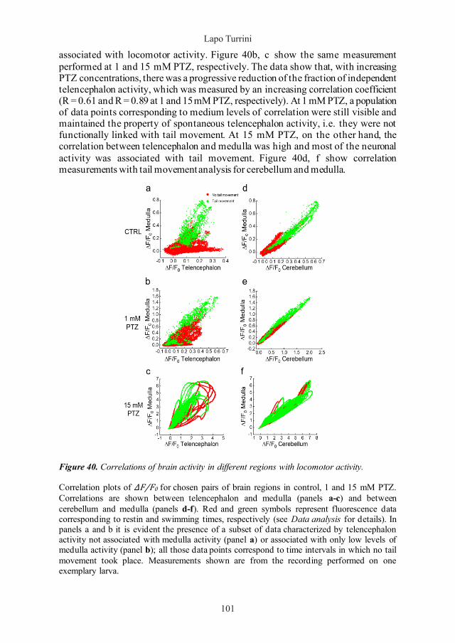
Lapo Turrini
100
mM PTZ) and rates. Figure 39c, d show the effects of PTZ on tail movement. Overall, the distributions of tail movement amplitudes (Fig.39c) demonstrate that PTZ most evidently induced seizures at 15 mM concentration, characterized by large tail swings (with amplitudes larger than 0,4 mm and up to 2.2 mm on our scale, where neither control nor 1 mM PTZ exhibited any event). These convulsive bursts are followed by a static phase, accounting for the lower average tail beat frequency in 15 mM PTZ compared to control and 1 mM (Fig.39d).
Figure 39. Distributions of brain activity and tail movement.
a, b. Bars represent average peak amplitude and average peak frequency, respectively, in the four brain regions highlighted in Figure 35a, for the three different conditions tested (0, 1 and 15 mM PTZ). Error is SEM. N = 3 larvae of 4 dpf for each experimental condition. c, d. Distribution of tail movement amplitude and average frequency for the three experimental condition tested (*, p = 0.0210; **, p = 0.0086, t-test of. N = 3 larvae of 4 dpf per condition. Error is STD.
We then analysed the correlations between neuronal activities in different brain regions with tail movement. We first considered the correlation between telencephalon and medulla, which was observed to be low in control condition and low PTZ concentrations (see Figure 37).
Figure 40a shows correlation in one typical recording performed without PTZ. The data confirmed the presence of a significant fraction of telencephalon activity not correlated with medulla, as quantitatively demonstrated also by the low correlation coefficient (R = 0.35). In order to assess the correlation of any brain activity with tail movement, we identified points in the fluorescence trace occurring during movement and plotted them with green symbols in the figure, while red symbols represent brain activity not associated with movement. We noticed that the independent telencephalon activity was not associated with any tail movement, while neuronal spiking occurring in the telencephalon synchronously with that of medulla was
101
associated with locomotor activity. Figure 40b, c show the same measurement performed at 1 and 15 mM PTZ, respectively. The data show that, with increasing PTZ concentrations, there was a progressive reduction of the fraction of independent telencephalon activity, which was measured by an increasing correlation coefficient (R = 0.61 and R = 0.89 at 1 and 15 mM PTZ, respectively). At 1 mM PTZ, a population of data points corresponding to medium levels of correlation were still visible and maintained the property of spontaneous telencephalon activity, i.e. they were not functionally linked with tail movement. At 15 mM PTZ, on the other hand, the correlation between telencephalon and medulla was high and most of the neuronal activity was associated with tail movement. Figure 40d, f show correlation measurements with tail movement analysis for cerebellum and medulla.
Figure 40. Correlations of brain activity in different regions with locomotor activity.
Correlation plots of ΔF/F for chosen pairs of brain regions in control, 1 and 15 mM PTZ. Correlations are shown between telencephalon and medulla (panels a-c) and between cerebellum and medulla (panels d-f). Red and green symbols represent fluorescence data corresponding to restin and swimming times, respectively (see Data analysis for details). In panels a and b it is evident the presence of a subset of data characterized by telencephalon activity not associated with medulla activity (panel a) or associated with only low levels of medulla activity (panel b); all those data points correspond to time intervals in which no tail movement took place. Measurements shown are from the recording performed on one exemplary larva.
101

Real-time whole-brain functional imaging of zebrafish neuronal activity
102
In this case, we could observe complete correlation of the two areas in all conditions (R = 0.94, 0.98 and 0.98 at 0, 1 and 15 mM PTZ, respectively) and a tight link between activity in these areas and locomotor activity.
A systematic characterization of the correlation of activity across all the four brain areas (for left and right hemisphere, Figure 41) confirmed the observation that increasing PTZ concentrations induce seizures consisting of highly correlated activity across the whole brain. At low (1 mM) PTZ concentration and in control conditions, on the other hand, we could observe the progressive loss of correlation along the rostro-caudal axis, with the telencephalon being the region which less correlates with the others. In all conditions, we observed a high correlation between left and right side of each region. We also observed that after onset of PTZ effect, correlations maintained their characteristic patterns for the whole duration of our measurements. These results are in line with previously observed whole-brain activation induced by PTZ (Fosque et al., 2015;Randlett et al., 2015) and with the common use of PTZ at 10–15 mM concentration to induce generalized seizures in the larva.
Figure 41. Cross-correlations maps of activity in different brain regions.
a. Regions of interest selected for analysis are shown overlaid with the wide-field fluorescence image. Scale bar: 100 µm. b. Cross-correlation matrices (see Data analysis) measured at different time intervals during one-hour recording in different conditions, as indicated. Each matrix shows color-coded averaged cross-correlation coefficients of N = 3 larvae of 4 dpf, exposed to the same condition, during the same timeframe.
15.4 High-throughput combined fluorescence and behavioural recordings
One of the main advantages of zebrafish in pharmacological research is the possibility of performing high-throughput drug screenings. The data shown in Figures 36-37 demonstrate that measurements of neuronal activity can complement behavioural measurements by providing information on activity alterations not always linked to
103
altered swimming behaviour of the larva. To this purpose, we implemented fluorescence measurements in a wide-field configuration at low magnification, enabling imaging over a large area (~50 cm2). With this optical system, we could simultaneously measure GCaMP6s fluorescence and larva position from 61 larvae in parallel, testing ten different experimental conditions with statistics of 5-6 larvae per condition. We chose to reproduce some previously tested conditions (i.e. 0, 1 and 15 mM PTZ treatment, VPA, tricaine and TTX treatments in the presence of 15 mM PTZ), together with a test on the effects of two compounds acting on synaptic transmission and previously shown to alter PTZ-induced seizures as measured with electrical recordings (Baraban et al., 2005): kynurenate (a non-specific blocker of postsynaptic glutamate receptors, which was shown to reduce seizure amplitudes) and Baclofen (a GABAB receptor agonist, which was shown to increase the amplitude of seizures). For an overall view of larva behaviour and fluorescence in each well, we produced a maximum intensity projection (MIP) of 45 minutes (Fig.42a), after one hour of drugs exposure.
102

Lapo Turrini
102
In this case, we could observe complete correlation of the two areas in all conditions (R = 0.94, 0.98 and 0.98 at 0, 1 and 15 mM PTZ, respectively) and a tight link between activity in these areas and locomotor activity.
A systematic characterization of the correlation of activity across all the four brain areas (for left and right hemisphere, Figure 41) confirmed the observation that increasing PTZ concentrations induce seizures consisting of highly correlated activity across the whole brain. At low (1 mM) PTZ concentration and in control conditions, on the other hand, we could observe the progressive loss of correlation along the rostro-caudal axis, with the telencephalon being the region which less correlates with the others. In all conditions, we observed a high correlation between left and right side of each region. We also observed that after onset of PTZ effect, correlations maintained their characteristic patterns for the whole duration of our measurements. These results are in line with previously observed whole-brain activation induced by PTZ (Fosque et al., 2015;Randlett et al., 2015) and with the common use of PTZ at 10–15 mM concentration to induce generalized seizures in the larva.
Figure 41. Cross-correlations maps of activity in different brain regions.
a. Regions of interest selected for analysis are shown overlaid with the wide-field fluorescence image. Scale bar: 100 µm. b. Cross-correlation matrices (see Data analysis) measured at different time intervals during one-hour recording in different conditions, as indicated. Each matrix shows color-coded averaged cross-correlation coefficients of N = 3 larvae of 4 dpf, exposed to the same condition, during the same timeframe.
15.4 High-throughput combined fluorescence and behavioural recordings
One of the main advantages of zebrafish in pharmacological research is the possibility of performing high-throughput drug screenings. The data shown in Figures 36-37 demonstrate that measurements of neuronal activity can complement behavioural measurements by providing information on activity alterations not always linked to
103
altered swimming behaviour of the larva. To this purpose, we implemented fluorescence measurements in a wide-field configuration at low magnification, enabling imaging over a large area (~50 cm2). With this optical system, we could simultaneously measure GCaMP6s fluorescence and larva position from 61 larvae in parallel, testing ten different experimental conditions with statistics of 5-6 larvae per condition. We chose to reproduce some previously tested conditions (i.e. 0, 1 and 15 mM PTZ treatment, VPA, tricaine and TTX treatments in the presence of 15 mM PTZ), together with a test on the effects of two compounds acting on synaptic transmission and previously shown to alter PTZ-induced seizures as measured with electrical recordings (Baraban et al., 2005): kynurenate (a non-specific blocker of postsynaptic glutamate receptors, which was shown to reduce seizure amplitudes) and Baclofen (a GABAB receptor agonist, which was shown to increase the amplitude of seizures). For an overall view of larva behaviour and fluorescence in each well, we produced a maximum intensity projection (MIP) of 45 minutes (Fig.42a), after one hour of drugs exposure.
103

Real-time whole-brain functional imaging of zebrafish neuronal activity
104
Figure 42. High-throughput combined fluorescence and behavioural assay.
a. Maximum intensity projection of a 13 minutes segment of two-hours recording. Well content: 1-6 control, 7-12 1 mM PTZ, 13-18 15 mM PTZ, 19-24 1 mM PTZ + 50 µM baclofen (BAC), 25-30 15 mM PTZ + 50 µM BAC, 31-36 15 mM PTZ + 5 µM tetrodotoxin (TTX), 37 fish water, 38 fish water + 2 mM kynurenate (KYN), 39-43 15 mM PTZ + 2 mM KYN, 44-49 16 mM PTZ + 5 mM valproic acid (VPA), 50-55 15 mM PTZ (after pre-incubation in 2 mM d-tubocurarine – D-TC – for 10 minutes before starting the measurement), 56-61 15 mM PTZ + 160 mg/L tricaine (TRIC). b, c. Average ΔF/F and swimming velocity for the different conditions tested. Error is SEM.
The figure immediately demonstrates the effects of increasing PTZ concentrations, as visible from an increased motility of the larvae at 1 mM PTZ (wells 7-12) compared to control (wells 1-6) and a further increase of motility, associated with a very large increase of fluorescence at 15 mM PTZ (wells 13-18). Introduction of Baclofen potentiated the fluorescence signal both at 1 (wells 19-24) and 15 mM PTZ (25-30). Tetrodotoxin (wells 31-36), on the other hand, completely suppressed neuronal activity, even in the presence of 15 mM PTZ, as show in Figure 35d, with consequent decrease of signal and larva paralysis. The effect of kynurenate (wells 39-43) was not apparent in the MIP analysis but became more evident in a subsequent quantitative analysis of ΔF/F and movement (Fig.42b-c). An important point to note in this type of assay is that some compounds (for example kynurenate) might display significant fluorescence at the wavelengths employed for GCaMP6s excitation and detection, as demonstrated by the background measured in the well containing only kynurenate (well 38) compared to fish water (well 37).
VPA showed its effectiveness in the MIP measurement (wells 44-49) where it decreased both larva motility and fluorescence in the presence of 15 mM PTZ. D-TC (wells 50-55) caused larva paralysis, but unfortunately often caused the death of the larvae at the concentration used. Finally, tricaine (wells 56-61) showed its anaesthetic effect in terms of both reduced fluorescence and motility of the larvae. The results of the high-throughput assay were quantified also by measuring the average ΔF/F (Fig.42b) and larva swimming velocity (Fig.42c) in all conditions tested. Velocities were calculated from trajectories shown in Figure 43.
Figure 43. Movement trajectories of larvae in high-throughput assay.
For each well, the coordinates of the centre of mass of the larva encephalon are plotted for a one-hour measurement. Colours refer to different pharmacological treatments (see legend). Scale bar: 7 mm.
105
Chapter 16 Bessel beam illumination as a means to reduce artefacts in quantitative functional studies using light-sheet microscopy
To improve the spatial resolution of neuronal functional imaging, with respect to the wide-field fluorescence recordings just shown, we decided to perform light -sheet fluorescence microscopy (LSFM) measurements. LSFM, a technique that affords intrinsic optical sectioning, fast acquisition rates and low phototoxicity, represents the method of choice to perform high-speed functional imaging in the zebrafish larva brain. However, its very nature of uncoupled, perpendicular optical pathways for fluorescence excitation and detection entails a set of drawbacks unique to LSFM in the form of dark shadows that appear whenever the fluorescence-exciting light sheet is interrupted by scattering or absorbing obstacles (see LSFM: drawbacks and solutions), especially in the case of one-sided illumination. These refractive index heterogeneities, always present to some extent even in the intrinsically transparent zebrafish larva, have been shown to lead to a loss of spatial resolution and a concomitant degradation in sensitivity and contrast (Chen et al., 2017).
16.1 Streaking artefacts obscure microscopic features of interest
Aiming for an optical solution to streaking artefacts, we have implemented on a custom-made light-sheet microscope (see Microscopes) an alternative illumination path based on Bessel beams (Durnin et al., 1987). Figure 44 shows the effect of streaking artefacts. The image obtained using conventional Gaussian illumination (Fig.44a) shows degraded image homogeneity and dark shadows obscuring microscopic anatomical features of interest that are further illustrated in an inset detailing the hindbrain.
Notably, those same features remain clearly visible when using Bessel beam illumination (Fig. 44b). In order to quantify the extent of the area affected by strong striping, we calculated the normalised line profiles obtained over the entire width (along the illumination direction) of the image for Gauss and Bessel illumination22 respectively (Fig. 44c).
22 In order to perform direct pair-wise comparison between Gaussian and Bessel illumination acquisitions, the Bessel beam was co-aligned to the Gaussian one, thus having two superimposing light sheets. This procedure allowed minimising the eventual need to adjust larvae position in z in order to image exactly the same brain plane. Pairs of identical structures were followed in the larval brain to be sure to acquire the same exact plane with both illuminations.
104

104
Figure 42. High-throughput combined fluorescence and behavioural assay.
a. Maximum intensity projection of a 13 minutes segment of two-hours recording. Well content: 1-6 control, 7-12 1 mM PTZ, 13-18 15 mM PTZ, 19-24 1 mM PTZ + 50 µM baclofen (BAC), 25-30 15 mM PTZ + 50 µM BAC, 31-36 15 mM PTZ + 5 µM tetrodotoxin (TTX), 37 fish water, 38 fish water + 2 mM kynurenate (KYN), 39-43 15 mM PTZ + 2 mM KYN, 44-49 16 mM PTZ + 5 mM valproic acid (VPA), 50-55 15 mM PTZ (after pre-incubation in 2 mM d-tubocurarine – D-TC – for 10 minutes before starting the measurement), 56-61 15 mM PTZ + 160 mg/L tricaine (TRIC). b, c. Average ΔF/F and swimming velocity for the different conditions tested. Error is SEM.
The figure immediately demonstrates the effects of increasing PTZ concentrations, as visible from an increased motility of the larvae at 1 mM PTZ (wells 7-12) compared to control (wells 1-6) and a further increase of motility, associated with a very large increase of fluorescence at 15 mM PTZ (wells 13-18). Introduction of Baclofen potentiated the fluorescence signal both at 1 (wells 19-24) and 15 mM PTZ (25-30). Tetrodotoxin (wells 31-36), on the other hand, completely suppressed neuronal activity, even in the presence of 15 mM PTZ, as show in Figure 35d, with consequent decrease of signal and larva paralysis. The effect of kynurenate (wells 39-43) was not apparent in the MIP analysis but became more evident in a subsequent quantitative analysis of ΔF/F and movement (Fig.42b-c). An important point to note in this type of assay is that some compounds (for example kynurenate) might display significant fluorescence at the wavelengths employed for GCaMP6s excitation and detection, as demonstrated by the background measured in the well containing only kynurenate (well 38) compared to fish water (well 37).
VPA showed its effectiveness in the MIP measurement (wells 44-49) where it decreased both larva motility and fluorescence in the presence of 15 mM PTZ. D-TC (wells 50-55) caused larva paralysis, but unfortunately often caused the death of the larvae at the concentration used. Finally, tricaine (wells 56-61) showed its anaesthetic effect in terms of both reduced fluorescence and motility of the larvae. The results of the high-throughput assay were quantified also by measuring the average ΔF/F (Fig.42b) and larva swimming velocity (Fig.42c) in all conditions tested. Velocities were calculated from trajectories shown in Figure 43.
Figure 43. Movement trajectories of larvae in high-throughput assay.
For each well, the coordinates of the centre of mass of the larva encephalon are plotted for a one-hour measurement. Colours refer to different pharmacological treatments (see legend). Scale bar: 7 mm.
105
Chapter 16 Bessel beam illumination as a means to reduce artefacts in quantitative functional studies using light-sheet microscopy
To improve the spatial resolution of neuronal functional imaging, with respect to the wide-field fluorescence recordings just shown, we decided to perform light -sheet fluorescence microscopy (LSFM) measurements. LSFM, a technique that affords intrinsic optical sectioning, fast acquisition rates and low phototoxicity, represents the method of choice to perform high-speed functional imaging in the zebrafish larva brain. However, its very nature of uncoupled, perpendicular optical pathways for fluorescence excitation and detection entails a set of drawbacks unique to LSFM in the form of dark shadows that appear whenever the fluorescence-exciting light sheet is interrupted by scattering or absorbing obstacles (see LSFM: drawbacks and solutions), especially in the case of one-sided illumination. These refractive index heterogeneities, always present to some extent even in the intrinsically transparent zebrafish larva, have been shown to lead to a loss of spatial resolution and a concomitant degradation in sensitivity and contrast (Chen et al., 2017).
16.1 Streaking artefacts obscure microscopic features of interest
Aiming for an optical solution to streaking artefacts, we have implemented on a custom-made light-sheet microscope (see Microscopes) an alternative illumination path based on Bessel beams (Durnin et al., 1987). Figure 44 shows the effect of streaking artefacts. The image obtained using conventional Gaussian illumination (Fig.44a) shows degraded image homogeneity and dark shadows obscuring microscopic anatomical features of interest that are further illustrated in an inset detailing the hindbrain.
Notably, those same features remain clearly visible when using Bessel beam illumination (Fig. 44b). In order to quantify the extent of the area affected by strong striping, we calculated the normalised line profiles obtained over the entire width (along the illumination direction) of the image for Gauss and Bessel illumination22 respectively (Fig. 44c).
22 In order to perform direct pair-wise comparison between Gaussian and Bessel illumination acquisitions, the Bessel beam was co-aligned to the Gaussian one, thus having two superimposing light sheets. This procedure allowed minimising the eventual need to adjust larvae position in z in order to image exactly the same brain plane. Pairs of identical structures were followed in the larval brain to be sure to acquire the same exact plane with both illuminations. Lapo Turrini, Development of optical methods for real-time whole-brain functional imaging of zebrafish neuronal activity, © 2020 Author(s), content CC BY 4.0 International, metadata CC0 1.0 Universal, published by Firenze University Press (www.fupress.com), ISSN 2612-8020 (online), ISBN 978-88-5518-070-2 (PDF), DOI 10.36253/978-88-5518-070-2

Real-time whole-brain functional imaging of zebrafish neuronal activity
106
Figure 44. Shadow artefacts in zebrafish brain imaging.
a, b. Static shadows in the transverse plane of a 3 dpf Tg(elavl3:GCaMP6s) zebrafish larva imaged with Gaussian and Bessel beam illumination, respectively. Insets showing hindbrain details. Light blue arrow indicates light-sheet propagation. Scale bar: 50 µm. c. Normalised line profile averaged over the entire width of the image for Gaussian (grey) and Bessel beam illumination (blue) evidences the shadows as drops in the grey curve. d. Absolute difference of the line profiles in c and the resulting bar code when applying a threshold of 5%. With this threshold, 72.8% ± 12.5% was affected by streaking artefacts. n = 20 planes throughout the encephalon in N = 11 larvae of 4-5 dpf, error is standard deviation. e. Sensitivity of the affected area on the threshold. Each point is the average of n = 20 planes in N = 11 larvae of 4-5 dpf, error is SEM. f. The difference between the half of the larva proximal and distal to the light-sheet source is not statistically significant. p = 0.6467, paired t-test of n = 20 planes in N = 11 larvae of 4-5 dpf, error is SEM.
107
Drops in the line profile evidenced sharp decrease in fluorescence signal propagating along image width. The absolute difference between Gauss and Bessel line profile was calculated and further binarised (Fig.44d) with respect to a user-selected threshold23. This procedure led us to obtain a pattern similar to a bar code, with dark bands representing image portion whose intensity difference between Gauss and Bessel acquisition dropped below the set threshold. By superimposing this bar pattern to the original image, the percentage of area affected by streaking inhomogeneity was estimated. Using a threshold of 5% (on the difference between the line profiles obtained with the two different illuminations) we estimated that 72.8% ±12.5 % (error is standard deviation, n = 20 planes throughout the encephalon, N = 11 larvae) of the volume was affected by streaking. Clearly, the value calculated is strongly dependent on the threshold. Indeed, the higher the threshold you chose, the higher the difference between Gauss and Bessel line profiles is acceptable, the less area affected by shadows you obtain. The sensitivity of the area percentage on the threshold is reported in Figure 44e (using the same sample size, error is SEM). The percentage area when considering only the proximal or distal half of the zebrafish relative to the illumination direction shows no statistically relevant difference (Fig.44f, p = 0.6467, paired t-test of n = 20 planes in N = 11 larvae aged 4-5 dpf, error is SEM).
23 Basically, the threshold determined how much difference between Gauss and Bessel line profiles was acceptable.
106

Lapo Turrini
106
Figure 44. Shadow artefacts in zebrafish brain imaging.
a, b. Static shadows in the transverse plane of a 3 dpf Tg(elavl3:GCaMP6s) zebrafish larva imaged with Gaussian and Bessel beam illumination, respectively. Insets showing hindbrain details. Light blue arrow indicates light-sheet propagation. Scale bar: 50 µm. c. Normalised line profile averaged over the entire width of the image for Gaussian (grey) and Bessel beam illumination (blue) evidences the shadows as drops in the grey curve. d. Absolute difference of the line profiles in c and the resulting bar code when applying a threshold of 5%. With this threshold, 72.8% ± 12.5% was affected by streaking artefacts. n = 20 planes throughout the encephalon in N = 11 larvae of 4-5 dpf, error is standard deviation. e. Sensitivity of the affected area on the threshold. Each point is the average of n = 20 planes in N = 11 larvae of 4-5 dpf, error is SEM. f. The difference between the half of the larva proximal and distal to the light-sheet source is not statistically significant. p = 0.6467, paired t-test of n = 20 planes in N = 11 larvae of 4-5 dpf, error is SEM.
107
Drops in the line profile evidenced sharp decrease in fluorescence signal propagating along image width. The absolute difference between Gauss and Bessel line profile was calculated and further binarised (Fig.44d) with respect to a user-selected threshold23. This procedure led us to obtain a pattern similar to a bar code, with dark bands representing image portion whose intensity difference between Gauss and Bessel acquisition dropped below the set threshold. By superimposing this bar pattern to the original image, the percentage of area affected by streaking inhomogeneity was estimated. Using a threshold of 5% (on the difference between the line profiles obtained with the two different illuminations) we estimated that 72.8% ±12.5 % (error is standard deviation, n = 20 planes throughout the encephalon, N = 11 larvae) of the volume was affected by streaking. Clearly, the value calculated is strongly dependent on the threshold. Indeed, the higher the threshold you chose, the higher the difference between Gauss and Bessel line profiles is acceptable, the less area affected by shadows you obtain. The sensitivity of the area percentage on the threshold is reported in Figure 44e (using the same sample size, error is SEM). The percentage area when considering only the proximal or distal half of the zebrafish relative to the illumination direction shows no statistically relevant difference (Fig.44f, p = 0.6467, paired t-test of n = 20 planes in N = 11 larvae aged 4-5 dpf, error is SEM).
23 Basically, the threshold determined how much difference between Gauss and Bessel line profiles was acceptable.
107

Real-time whole-brain functional imaging of zebrafish neuronal activity
108
Figure 45. Haemodynamic flickering in zebrafish brain imaging.
a. Transverse plane of a 4 dpf Tg(elavl3:H2B-GCaMP6s) zebrafish larva imaged with Gaussian illumination. Image is the maximum intensity projection, over 0.3 s time-lapse. Inset highlights the presence of a large blood vessel in which, during MIP time window, one single erythrocyte is flowing. Owing to the nature of the projection, the passing red blood cell is visible at different position along the vessel (yellow arrowheads). At any new position taken, the erythrocyte absorbs or scatters the excitation light, casting a tiny shadow along the direction of propagation of the light sheet (light blue arrow). b. Projection of the standard deviation over 1 s of time-lapse recording on a transverse plane of a 4 dpf zebrafish larva imaged with Gaussian illumination. Yellow arrowheads pointing at a large blood vessel. The flow of blood cells inside the vessel produces dynamic shadows that generate a corresponding area of high standard deviation of the fluorescence intensity, downstream along the light-sheet propagation direction. c. Projections of the standard deviation on a transverse plane of a 4 dpf zebrafish larva, sequentially imaged with Gaussian illumination (left) and Bessel beam illumination (right), displayed on the same brightness scale. d. Quantification of the area affected by flickering for Gaussian (23.8% ± 6.5%) and Bessel beam illumination (0.8% ± 0.5%). p < 0.0001, paired t-test of n = 18 planes in N = 10 larvae of 4-5 dpf, error is SEM. All measurements presented in this figure were conducted under tricaine (160 mg/L) treatment in order to evaluate only fluorescence changes due to dynamic streaking artefact. Scale bars: 50 µm. Calibration bar refers to both panels b and c.
Furthermore, when the obstacles that obstruct the light sheet are not static, the shadows produced move accordingly. Among these moving particles, for sure, a key role is played by blood cells. As early as three days post fertilization (dpf), fully formed blood vessels can be easily distinguished by the flow of individual blood cells (Fig.45a, inset yellow arrowheads). Dynamic shadowing caused by the movement of red blood cells leads to a fluctuation of fluorescence intensity independent from neuronal activity, causing an artefact here termed flickering. Haemodynamic absorption (Chen et al., 2014;Ma et al., 2016) of the light sheet can be particularly problematic for in vivo Ca2+ imaging as it represents a multiplicative noise source (Ma et al., 2016) and therefore has the potential to modulate significantly the sensitivity to fluorescence variations related to neuronal activity in adjacent neurons. A projection of the standard deviation over ~1 s of recording (Fig.45b) clearly evidences blood vessels by superimposing the trajectories of blood cells and further highlights the strong variations in grey values in corresponding adjacent regions. Notably, when displayed on the same brightness scale, the corresponding areas are free of strong flickering when using Bessel beam illumination (Fig.45c).
16.2 Flickering quantification
In order to evaluate to which extent flickering potentially masks or even falsifies neuronal activity when using Gaussian illumination, we directly compared each quantification with its Bessel beam counterpart. All measurements aiming to quantify the flickering issue were conducted on larvae treated with tricaine (160 mg/L) to globally lower neuronal activity (Attili and Hughes, 2014) (see also Fig. 35c), ensuring that any changes in baseline fluorescence were exclusively due to dynamic
109
shadowing and not neuronal activity. First, based on an approach employing standard deviation projections (see Data analysis, Fig.33), we quantified the percentage area that on average was affected by flickering in each imaged brain plane. We found it to be 23.8 % ± 6.5 % for Gaussian and 0.8 % ± 0.5 % for Bessel beam illumination (Fig.45d, error is SEM, p < 0.0001, paired t-test, n = 18 planes in N = 10 larvae of 4-5 dpf).
Figure 46. Flickering quantification.
a. ΔF/F baseline traces of three representative neurons chosen in different position in a transverse plane of a 4 dpf Tg(elavl3:H2B-GCaMP6s) zebrafish larva treated with 160 mg/L tricaine. b. Average standard deviation (STD) of baseline traces of neurons showing no activity from larvae treated with 160 mg/L tricaine (p < 0.0001, paired t-test, n = 625 cells in N = 7 larvae of 4-5 dpf, error is SEM). c. Exemplary ΔF/F traces measured with Bessel beam illumination during spontaneous neuronal activity. Straight horizontal lines represent the average noise level measured for Gauss (grey) and Bessel (blue). Triangles show peaks above noise level for Gaussian (grey) and Bessel beam illumination (blue). Peaks with prominence below threshold were discarded (red triangle). d. Average peaks per minute detected above noise level using appropriate thresholding to exclude Gaussian and Bessel baseline noise (p < 0.0001, paired t-test, n = 586 in N = 1 larva of 4 dpf, error is SEM.).Scale bars in a, b are 0.1 ΔF/F and 30 s.
Due to the irregular flow of blood cells, the traversing excitation light sheet is either absorbed or scattered out of its trajectory such that the baseline fluorescence in adjacent neurons is no longer steadily generated, both because of direct shadowing of in-focus fluorophores and of spurious excitation of out-of-focus ones. Subsequently, we compared baseline ΔF/F traces of pairwise identical neurons, imaged with either Gaussian or Bessel beam, located in areas affected by flickering. Figure 46a shows representative ΔF/F traces of three neurons chosen in different positions of a
108

Lapo Turrini
108
Figure 45. Haemodynamic flickering in zebrafish brain imaging.
a. Transverse plane of a 4 dpf Tg(elavl3:H2B-GCaMP6s) zebrafish larva imaged with Gaussian illumination. Image is the maximum intensity projection, over 0.3 s time-lapse. Inset highlights the presence of a large blood vessel in which, during MIP time window, one single erythrocyte is flowing. Owing to the nature of the projection, the passing red blood cell is visible at different position along the vessel (yellow arrowheads). At any new position taken, the erythrocyte absorbs or scatters the excitation light, casting a tiny shadow along the direction of propagation of the light sheet (light blue arrow). b. Projection of the standard deviation over 1 s of time-lapse recording on a transverse plane of a 4 dpf zebrafish larva imaged with Gaussian illumination. Yellow arrowheads pointing at a large blood vessel. The flow of blood cells inside the vessel produces dynamic shadows that generate a corresponding area of high standard deviation of the fluorescence intensity, downstream along the light-sheet propagation direction. c. Projections of the standard deviation on a transverse plane of a 4 dpf zebrafish larva, sequentially imaged with Gaussian illumination (left) and Bessel beam illumination (right), displayed on the same brightness scale. d. Quantification of the area affected by flickering for Gaussian (23.8% ± 6.5%) and Bessel beam illumination (0.8% ± 0.5%). p < 0.0001, paired t-test of n = 18 planes in N = 10 larvae of 4-5 dpf, error is SEM. All measurements presented in this figure were conducted under tricaine (160 mg/L) treatment in order to evaluate only fluorescence changes due to dynamic streaking artefact. Scale bars: 50 µm. Calibration bar refers to both panels b and c.
Furthermore, when the obstacles that obstruct the light sheet are not static, the shadows produced move accordingly. Among these moving particles, for sure, a key role is played by blood cells. As early as three days post fertilization (dpf), fully formed blood vessels can be easily distinguished by the flow of individual blood cells (Fig.45a, inset yellow arrowheads). Dynamic shadowing caused by the movement of red blood cells leads to a fluctuation of fluorescence intensity independent from neuronal activity, causing an artefact here termed flickering. Haemodynamic absorption (Chen et al., 2014;Ma et al., 2016) of the light sheet can be particularly problematic for in vivo Ca2+ imaging as it represents a multiplicative noise source (Ma et al., 2016) and therefore has the potential to modulate significantly the sensitivity to fluorescence variations related to neuronal activity in adjacent neurons. A projection of the standard deviation over ~1 s of recording (Fig.45b) clearly evidences blood vessels by superimposing the trajectories of blood cells and further highlights the strong variations in grey values in corresponding adjacent regions. Notably, when displayed on the same brightness scale, the corresponding areas are free of strong flickering when using Bessel beam illumination (Fig.45c).
16.2 Flickering quantification
In order to evaluate to which extent flickering potentially masks or even falsifies neuronal activity when using Gaussian illumination, we directly compared each quantification with its Bessel beam counterpart. All measurements aiming to quantify the flickering issue were conducted on larvae treated with tricaine (160 mg/L) to globally lower neuronal activity (Attili and Hughes, 2014) (see also Fig. 35c), ensuring that any changes in baseline fluorescence were exclusively due to dynamic
109
shadowing and not neuronal activity. First, based on an approach employing standard deviation projections (see Data analysis, Fig.33), we quantified the percentage area that on average was affected by flickering in each imaged brain plane. We found it to be 23.8 % ± 6.5 % for Gaussian and 0.8 % ± 0.5 % for Bessel beam illumination (Fig.45d, error is SEM, p < 0.0001, paired t-test, n = 18 planes in N = 10 larvae of 4-5 dpf).
Figure 46. Flickering quantification.
a. ΔF/F baseline traces of three representative neurons chosen in different position in a transverse plane of a 4 dpf Tg(elavl3:H2B-GCaMP6s) zebrafish larva treated with 160 mg/L tricaine. b. Average standard deviation (STD) of baseline traces of neurons showing no activity from larvae treated with 160 mg/L tricaine (p < 0.0001, paired t-test, n = 625 cells in N = 7 larvae of 4-5 dpf, error is SEM). c. Exemplary ΔF/F traces measured with Bessel beam illumination during spontaneous neuronal activity. Straight horizontal lines represent the average noise level measured for Gauss (grey) and Bessel (blue). Triangles show peaks above noise level for Gaussian (grey) and Bessel beam illumination (blue). Peaks with prominence below threshold were discarded (red triangle). d. Average peaks per minute detected above noise level using appropriate thresholding to exclude Gaussian and Bessel baseline noise (p < 0.0001, paired t-test, n = 586 in N = 1 larva of 4 dpf, error is SEM.).Scale bars in a, b are 0.1 ΔF/F and 30 s.
Due to the irregular flow of blood cells, the traversing excitation light sheet is either absorbed or scattered out of its trajectory such that the baseline fluorescence in adjacent neurons is no longer steadily generated, both because of direct shadowing of in-focus fluorophores and of spurious excitation of out-of-focus ones. Subsequently, we compared baseline ΔF/F traces of pairwise identical neurons, imaged with either Gaussian or Bessel beam, located in areas affected by flickering. Figure 46a shows representative ΔF/F traces of three neurons chosen in different positions of a
109

Real-time whole-brain functional imaging of zebrafish neuronal activity
110
transverse plane of the encephalon of a 4 dpf tg(elavl3:H2B-GCaMP6s) zebrafish larva. Different positions in the encephalon display different levels of baseline noise; however, in general, the noise obtained in Bessel traces was consistently lower than that in traces obtained with Gaussian illumination. Quantified by their standard deviation, we analysed traces measured with Gaussian and Bessel beam illumination respectively to obtain the level of baseline noise in the absence of neuronal activity (Fig.46b). The baseline noise was 19.65% ± 0.18% of ΔF/F for Gaussian and 3.90% ± 0.07% for Bessel beam illumination (p < 0.0001, paired t-test, n = 625 cells, 15 time-lapses at various depths in N = 7 larvae of 4-5 dpf, error is SEM) constituting a five-fold increase in sensitivity.
16.3 Impact of flickering on neuronal activity measurements
Once quantified the average noise typical of Gaussian and Bessel beam measurements, we wanted to test to which extent the noise level affected neuronal activity identification in both measurement conditions. To this end, we devised a peak counting routine (Fig. 46c, see Data analysis) which counted peaks above Gaussian baseline noise (grey triangles) and again above Bessel beam baseline noise (blue triangles) on identical traces obtained with Bessel beam illumination. Peaks of sub-threshold prominence (red triangle) were discarded. The total number of peaks per minute detected above their respective baseline noise levels are reported in Figure 46d (p < 0.0001, paired t-test, n = 586 cells, in N=1 larva, error is SEM). Cells were located at 12 different depths throughout the encephalon of a 4 dpf larva. Whereas on average 6.6 peaks per minute could be detected above Bessel beam noise levels, only 0.5 peaks per minute were high enough to surpass the Gaussian baseline noise. This means that, statistically, if a given cell were to be located in an area affected by flickering, then less than 1 out of 12 peaks would be detected due to the higher associated baseline noise when using Gaussian compared to Bessel beam illumination. To further illustrate the influence of increased baseline noise on ΔF/F traces, we generated random white noise of an amplitude corresponding to the Gaussian and Bessel baseline noise respectively and multiplied it pairwise to traces obtained with Bessel beam illumination (Fig.47a).
The native data set without synthetic noise was considered as ground truth and allowed an absolute comparison between Gaussian and Bessel beam illumination. The absolute cross correlation coefficients reported in Figure 47b reveal that, while the mean of the Gaussian and native data set differ significantly (0.0978 vs 0.1309), the difference between the mean of the Bessel and the native data set is not statistically significant (0.1308 vs 0.1309) (p < 0.0001, t-test, n = 277885 corresponding to 746 cells in N=1 larva, error is too small to be displayed). Next, the difference in cross correlation coefficients between the native traces and the traces with synthetic noises was calculated. The histograms of these distributions give some important insights; whereas the mean value represents the bias of each modality, the standard deviation gives a measure of its accuracy. For Gaussian illumination, we obtained a mean value of 0.0127 whereas this value is 5.29·10-5 for Bessel beam illumination. This result indicates the introduction of a systematic error by Gaussian illumination that is
111
approximately one tenth of the average absolute correlation coefficient. Furthermore, the standard deviations of the histograms give a direct measure of the random error introduced by each method and therefore a measure of accuracy. The standard deviation was 0.0682 for Gaussian and 0.0033 for Bessel beam illumination (Fig.47c) which constitutes a 20-fold increase in accuracy compared to Gaussian illumination.
Figure 47. Effect of random synthetic noise on neuronal activity cross-correlation.
a. The baseline noise levels calculated in Fig. 46b was used as amplitude to generate a random white noise which was point-wise multiplied to 746 ΔF/F traces obtained with Bessel beam modality. By defining the 746 synthetic noise-free traces as ground truth (native), we obtained three data sets that we compared by respective cross correlation. b. Average absolute cross-correlation coefficient (CCC) (p < 0.0001, t-test, n = 277885 corresponding to 746 cells in N = 1 larva of 4 dpf, error is SEM, too small to be shown, NS: not significant). c. STD of the difference in cross-correlation coefficients between the native traces and the same traces with multiplied noise (p < 0.0001, paired t -test, n = 277885 corresponding to 746 cells in N = 1 larva of 4 dpf).
16.4 Flickering artefacts mask neuronal correlations
After showing that the contamination with both systematic and random errors is significantly higher when using Gaussian beam compared to Bessel beams, we performed measurements of spontaneous neuronal activity in the presence of flickering.
As indicated in Figure 48a, b, several cells have been manually selected in the hindbrain of a 4 dpf larva to generate a scenario in which spurious correlations due to flickering significantly alter the correlation amongst cells in a circuit. The red and blue cells where chosen in an area determined by the methodology described in Figure 45d and corresponded to lines in which nearby flowing blood cells cast alternating
110

Lapo Turrini
110
transverse plane of the encephalon of a 4 dpf tg(elavl3:H2B-GCaMP6s) zebrafish larva. Different positions in the encephalon display different levels of baseline noise; however, in general, the noise obtained in Bessel traces was consistently lower than that in traces obtained with Gaussian illumination. Quantified by their standard deviation, we analysed traces measured with Gaussian and Bessel beam illumination respectively to obtain the level of baseline noise in the absence of neuronal activity (Fig.46b). The baseline noise was 19.65% ± 0.18% of ΔF/F for Gaussian and 3.90% ± 0.07% for Bessel beam illumination (p < 0.0001, paired t-test, n = 625 cells, 15 time-lapses at various depths in N = 7 larvae of 4-5 dpf, error is SEM) constituting a five-fold increase in sensitivity.
16.3 Impact of flickering on neuronal activity measurements
Once quantified the average noise typical of Gaussian and Bessel beam measurements, we wanted to test to which extent the noise level affected neuronal activity identification in both measurement conditions. To this end, we devised a peak counting routine (Fig. 46c, see Data analysis) which counted peaks above Gaussian baseline noise (grey triangles) and again above Bessel beam baseline noise (blue triangles) on identical traces obtained with Bessel beam illumination. Peaks of sub-threshold prominence (red triangle) were discarded. The total number of peaks per minute detected above their respective baseline noise levels are reported in Figure 46d (p < 0.0001, paired t-test, n = 586 cells, in N=1 larva, error is SEM). Cells were located at 12 different depths throughout the encephalon of a 4 dpf larva. Whereas on average 6.6 peaks per minute could be detected above Bessel beam noise levels, only 0.5 peaks per minute were high enough to surpass the Gaussian baseline noise. This means that, statistically, if a given cell were to be located in an area affected by flickering, then less than 1 out of 12 peaks would be detected due to the higher associated baseline noise when using Gaussian compared to Bessel beam illumination. To further illustrate the influence of increased baseline noise on ΔF/F traces, we generated random white noise of an amplitude corresponding to the Gaussian and Bessel baseline noise respectively and multiplied it pairwise to traces obtained with Bessel beam illumination (Fig.47a).
The native data set without synthetic noise was considered as ground truth and allowed an absolute comparison between Gaussian and Bessel beam illumination. The absolute cross correlation coefficients reported in Figure 47b reveal that, while the mean of the Gaussian and native data set differ significantly (0.0978 vs 0.1309), the difference between the mean of the Bessel and the native data set is not statistically significant (0.1308 vs 0.1309) (p < 0.0001, t-test, n = 277885 corresponding to 746 cells in N=1 larva, error is too small to be displayed). Next, the difference in cross correlation coefficients between the native traces and the traces with synthetic noises was calculated. The histograms of these distributions give some important insights; whereas the mean value represents the bias of each modality, the standard deviation gives a measure of its accuracy. For Gaussian illumination, we obtained a mean value of 0.0127 whereas this value is 5.29·10-5 for Bessel beam illumination. This result indicates the introduction of a systematic error by Gaussian illumination that is
111
approximately one tenth of the average absolute correlation coefficient. Furthermore, the standard deviations of the histograms give a direct measure of the random error introduced by each method and therefore a measure of accuracy. The standard deviation was 0.0682 for Gaussian and 0.0033 for Bessel beam illumination (Fig.47c) which constitutes a 20-fold increase in accuracy compared to Gaussian illumination.
Figure 47. Effect of random synthetic noise on neuronal activity cross-correlation.
a. The baseline noise levels calculated in Fig. 46b was used as amplitude to generate a random white noise which was point-wise multiplied to 746 ΔF/F traces obtained with Bessel beam modality. By defining the 746 synthetic noise-free traces as ground truth (native), we obtained three data sets that we compared by respective cross correlation. b. Average absolute cross-correlation coefficient (CCC) (p < 0.0001, t-test, n = 277885 corresponding to 746 cells in N = 1 larva of 4 dpf, error is SEM, too small to be shown, NS: not significant). c. STD of the difference in cross-correlation coefficients between the native traces and the same traces with multiplied noise (p < 0.0001, paired t -test, n = 277885 corresponding to 746 cells in N = 1 larva of 4 dpf).
16.4 Flickering artefacts mask neuronal correlations
After showing that the contamination with both systematic and random errors is significantly higher when using Gaussian beam compared to Bessel beams, we performed measurements of spontaneous neuronal activity in the presence of flickering.
As indicated in Figure 48a, b, several cells have been manually selected in the hindbrain of a 4 dpf larva to generate a scenario in which spurious correlations due to flickering significantly alter the correlation amongst cells in a circuit. The red and blue cells where chosen in an area determined by the methodology described in Figure 45d and corresponded to lines in which nearby flowing blood cells cast alternating
111

Real-time whole-brain functional imaging of zebrafish neuronal activity
112
shadows, whereas the yellow cells have been randomly chosen among a circuit of cells that showed strong spontaneous activity.
Figure 48. Case study of the effect of haemodynamic artefact on neuronal activity cross-correlation.
a. Transverse plane of a 4 dpf Tg(elavl3:H2B-GCaMP6s) zebrafish larva imaged with Gaussian illumination. Indicated are cells located on two adjacent excitation lines (red, blue) and randomly in the hindbrain as part of an active network (yellow, see also zoomed view b, scale bar: 25 µm). c. Exemplary activity traces of cells marked in yellow in a,b measured with Gaussian (grey) and Bessel beam illumination (blue). Scale bar: 0.1 ΔF/F and 30 s. d. Cross-correlation matrix of neuronal activity of cells measured with Gaussian (lower triangular matrix) and Bessel beam illumination (upper triangular matrix). e. Average cross-correlation coefficient (CCC) of yellow/yellow quadrant (p < 0.0001, paired t-test, n = 91 in N = 1 larva of 4 dpf, error is SEM).
113
It is apparent from the correlation matrix (Fig.48d) that, when using Gaussian illumination, a strong correlation between cells on one line (sector marked ◼◼ in the correlation matrix) can be observed, which strongly anti-correlates with cells from the line immediately next to it (◼◼), an obvious haemodynamic artefact. Notably, when using Bessel beam illumination this strong spurious correlation was not observed (average cross correlation -0.571 ± 0.025 for Gauss versus -0.013 ± 0.023 for Bessel beam illumination, n = 55, error is SEM). Exemplary traces of spontaneous activity outside an area strongly affected by flickering (cells marked yellow) are shown in Figure 48c. It is worthwhile pointing out, that when looking at correlations entirely outside flickering areas (◼◼), average correlation obtained with Gaussian beams was 0.576 ± 0.020 and 0.660 ± 0.017 (an increase of 15%, n = 91) for Bessel beams (Fig.48e). This result demonstrates that even when steering clear of problematic areas with evident strong flickering, correlations of neuronal activity can be significantly affected by residual flickering, less evident to the human eye, when using Gaussian illumination. Since Bessel beams have a fivefold increased sensitivity to calcium transients compared to Gaussian beams, they are more likely to detect calcium transients in multiple functionally connected cells and this leads to a higher average correlation as seen in Figure 48e.
112

Lapo Turrini
112
shadows, whereas the yellow cells have been randomly chosen among a circuit of cells that showed strong spontaneous activity.
Figure 48. Case study of the effect of haemodynamic artefact on neuronal activity cross-correlation.
a. Transverse plane of a 4 dpf Tg(elavl3:H2B-GCaMP6s) zebrafish larva imaged with Gaussian illumination. Indicated are cells located on two adjacent excitation lines (red, blue) and randomly in the hindbrain as part of an active network (yellow, see also zoomed view b, scale bar: 25 µm). c. Exemplary activity traces of cells marked in yellow in a,b measured with Gaussian (grey) and Bessel beam illumination (blue). Scale bar: 0.1 ΔF/F and 30 s. d. Cross-correlation matrix of neuronal activity of cells measured with Gaussian (lower triangular matrix) and Bessel beam illumination (upper triangular matrix). e. Average cross-correlation coefficient (CCC) of yellow/yellow quadrant (p < 0.0001, paired t-test, n = 91 in N = 1 larva of 4 dpf, error is SEM).
113
It is apparent from the correlation matrix (Fig.48d) that, when using Gaussian illumination, a strong correlation between cells on one line (sector marked ◼◼ in the correlation matrix) can be observed, which strongly anti-correlates with cells from the line immediately next to it (◼◼), an obvious haemodynamic artefact. Notably, when using Bessel beam illumination this strong spurious correlation was not observed (average cross correlation -0.571 ± 0.025 for Gauss versus -0.013 ± 0.023 for Bessel beam illumination, n = 55, error is SEM). Exemplary traces of spontaneous activity outside an area strongly affected by flickering (cells marked yellow) are shown in Figure 48c. It is worthwhile pointing out, that when looking at correlations entirely outside flickering areas (◼◼), average correlation obtained with Gaussian beams was 0.576 ± 0.020 and 0.660 ± 0.017 (an increase of 15%, n = 91) for Bessel beams (Fig.48e). This result demonstrates that even when steering clear of problematic areas with evident strong flickering, correlations of neuronal activity can be significantly affected by residual flickering, less evident to the human eye, when using Gaussian illumination. Since Bessel beams have a fivefold increased sensitivity to calcium transients compared to Gaussian beams, they are more likely to detect calcium transients in multiple functionally connected cells and this leads to a higher average correlation as seen in Figure 48e.
113

115
Chapter 17 3D optical mapping of zebrafish neuronal activity with single cell resolution by Bessel beam illumination light-sheet microscopy
Once assessed the effectiveness of Bessel beam illumination in reducing artefacts arising from haemodynamic absorption and scattering in zebrafish functional imaging, we used this method to perform faithful measurements of zebrafish spontaneous and convulsive neuronal activity. In details, we performed light -sheet microscopy time-lapse recording on single planes of larval brain, progressively sampling most of the encephalon depth. In these measurements, we used Tg(elavl3:H2B-GCaMP6s) albino zebrafish larvae expressing the Ca2+ reporter in the nucleus of all CNS neurons. The nuclear localization of the indicator allowed us to perform an automatic segmentation of each plane’s cells. Single cell analysis was then
performed, thus obtaining 2D heat maps (see Figure A3) in which the activity of each single neuron detected was represented as a colour-scaled symbol placed in the coordinates belonging to that particular cell (see Data analysis for details). Figure 49. Whole-brain neuron detection.
23 individual brain planes of a 4 dpf Tg(elavl3:H2B-GCaMP6s) zebrafish larva processed with The_Cell_Detector.m (see Data analysis) to detect neurons. Each image report detected neurons as single white dots. Above each plane image is reported the number of cells actually detected by the algorithm. The overall number of neurons detected over 23 planes was 77˙495. On average the script identified 73˙991 ± 3984 neurons (N = 3 larvae of 4 dpf, error is STD).
114

115
Chapter 17 3D optical mapping of zebrafish neuronal activity with single cell resolution by Bessel beam illumination light-sheet microscopy
Once assessed the effectiveness of Bessel beam illumination in reducing artefacts arising from haemodynamic absorption and scattering in zebrafish functional imaging, we used this method to perform faithful measurements of zebrafish spontaneous and convulsive neuronal activity. In details, we performed light -sheet microscopy time-lapse recording on single planes of larval brain, progressively sampling most of the encephalon depth. In these measurements, we used Tg(elavl3:H2B-GCaMP6s) albino zebrafish larvae expressing the Ca2+ reporter in the nucleus of all CNS neurons. The nuclear localization of the indicator allowed us to perform an automatic segmentation of each plane’s cells. Single cell analysis was then
performed, thus obtaining 2D heat maps (see Figure A3) in which the activity of each single neuron detected was represented as a colour-scaled symbol placed in the coordinates belonging to that particular cell (see Data analysis for details). Figure 49. Whole-brain neuron detection.
23 individual brain planes of a 4 dpf Tg(elavl3:H2B-GCaMP6s) zebrafish larva processed with The_Cell_Detector.m (see Data analysis) to detect neurons. Each image report detected neurons as single white dots. Above each plane image is reported the number of cells actually detected by the algorithm. The overall number of neurons detected over 23 planes was 77˙495. On average the script identified 73˙991 ± 3984 neurons (N = 3 larvae of 4 dpf, error is STD).
Lapo Turrini, Development of optical methods for real-time whole-brain functional imaging of zebrafish neuronal activity, © 2020 Author(s), content CC BY 4.0 International, metadata CC0 1.0 Universal, published by Firenze University Press (www.fupress.com), ISSN 2612-8020 (online), ISBN 978-88-5518-070-2 (PDF), DOI 10.36253/978-88-5518-070-2

Real-time whole-brain functional imaging of zebrafish neuronal activity
116
Methods applied allowed us to image and detect great part of the 100˙000 larval brain neurons. Figure 49 shows the result of the segmentation process performed on 23 individual planes of the brain of a 4 dpf zebrafish larva. We were able to detect a total number of 77˙495 neurons over a depth of 160 µm. On average (N = 3) our method allowed identifying 73˙991 ± 3984 individual neurons per brain, a result close to that (80˙000) obtained by recent breakthrough publications (Ahrens et al., 2013;Freeman et al., 2014;Vladimirov et al., 2014).
Figure 50. Bessel beam light-sheet microscopy 3D mapping of zebrafish neuronal activity.
3D maps of zebrafish brain activity with single neuron resolution in 0 mM (a), 1 mM (b) and 7.5 mM (c) PTZ. zy planes show a lateral projection of the encephalon, while xy a dorsal projection. Each dot composing the map represents colour-scaled activity of that particular neuron along the time of measurement (4 min). Images are displayed in the same brightness scale.
Figure 50 shows, on the same brightness scale, the 3D maps of activity of three larvae in 0 mM (a), 1 mM (b), and 7.5 mM PTZ (c), respectively, in a lateral (zy) and a dorsal (xy) view each. A zebrafish larva during spontaneous activity (Fig.50a) showed predominant clustered activation of telencephalic, diencephalic, cerebellar, and hindbrain neurons (see zy lateral view). In particular, most active hindbrain neurons were arranged in two clusters, symmetric with respect to the rostro-caudal y-axis (see xy dorsal view), which were superimposable to the already described hindbrain oscillator (Ahrens et al., 2013) (or anterior rhomboencephalic turning region – ARTR (Dunn et al., 2016b)), a region involved in the control of motor behaviour. Conversely, optic tectum showed very low levels of activations. Neuronal activity appeared mostly confined to the superficial layers of the encephalon (Fig.50a, lateral view). In contrast with control condition, 1 mM PTZ treated larva (Fig.50b) showed a more widespread overall activation, spanning all the hindbrain, from cerebellum to the
117
medulla. Telencephalic neuronal activity appeared increased, whereas diencephalic (habenula) activity showed no significant increase. Neurons of the optic tectum exhibited a slight raise in activity. Globally, with 1 mM PTZ administration, neuronal activity showed an increase along the medio-lateral (x) and rostro-caudal (y) direction, with no significant increase in the depth (z) of the brain (see Figure 50a, b, lateral and dorsal view). The action of 7.5 mM PTZ (Fig.50c) induced robust widespread depolarisations even in the deepest encephalic layers here imaged (see lateral view). In contrast with 0 and 1 mM PTZ conditions, habenula and optic tectum showed large burst of synchronous neuronal activity, revealed by a massive activation in the map. Superficial activation (see Figure 50, lateral view) was quantitatively very similar to that observed in 1 mM PTZ condition, apart for optic tectum activation which even in the most superficial layers appeared more pronounced.
116

Lapo Turrini
116
Methods applied allowed us to image and detect great part of the 100˙000 larval brain neurons. Figure 49 shows the result of the segmentation process performed on 23 individual planes of the brain of a 4 dpf zebrafish larva. We were able to detect a total number of 77˙495 neurons over a depth of 160 µm. On average (N = 3) our method allowed identifying 73˙991 ± 3984 individual neurons per brain, a result close to that (80˙000) obtained by recent breakthrough publications (Ahrens et al., 2013;Freeman et al., 2014;Vladimirov et al., 2014).
Figure 50. Bessel beam light-sheet microscopy 3D mapping of zebrafish neuronal activity.
3D maps of zebrafish brain activity with single neuron resolution in 0 mM (a), 1 mM (b) and 7.5 mM (c) PTZ. zy planes show a lateral projection of the encephalon, while xy a dorsal projection. Each dot composing the map represents colour-scaled activity of that particular neuron along the time of measurement (4 min). Images are displayed in the same brightness scale.
Figure 50 shows, on the same brightness scale, the 3D maps of activity of three larvae in 0 mM (a), 1 mM (b), and 7.5 mM PTZ (c), respectively, in a lateral (zy) and a dorsal (xy) view each. A zebrafish larva during spontaneous activity (Fig.50a) showed predominant clustered activation of telencephalic, diencephalic, cerebellar, and hindbrain neurons (see zy lateral view). In particular, most active hindbrain neurons were arranged in two clusters, symmetric with respect to the rostro-caudal y-axis (see xy dorsal view), which were superimposable to the already described hindbrain oscillator (Ahrens et al., 2013) (or anterior rhomboencephalic turning region – ARTR (Dunn et al., 2016b)), a region involved in the control of motor behaviour. Conversely, optic tectum showed very low levels of activations. Neuronal activity appeared mostly confined to the superficial layers of the encephalon (Fig.50a, lateral view). In contrast with control condition, 1 mM PTZ treated larva (Fig.50b) showed a more widespread overall activation, spanning all the hindbrain, from cerebellum to the
117
medulla. Telencephalic neuronal activity appeared increased, whereas diencephalic (habenula) activity showed no significant increase. Neurons of the optic tectum exhibited a slight raise in activity. Globally, with 1 mM PTZ administration, neuronal activity showed an increase along the medio-lateral (x) and rostro-caudal (y) direction, with no significant increase in the depth (z) of the brain (see Figure 50a, b, lateral and dorsal view). The action of 7.5 mM PTZ (Fig.50c) induced robust widespread depolarisations even in the deepest encephalic layers here imaged (see lateral view). In contrast with 0 and 1 mM PTZ conditions, habenula and optic tectum showed large burst of synchronous neuronal activity, revealed by a massive activation in the map. Superficial activation (see Figure 50, lateral view) was quantitatively very similar to that observed in 1 mM PTZ condition, apart for optic tectum activation which even in the most superficial layers appeared more pronounced.
117

119
Chapter 18 Fast whole-brain functional imaging by two-photon light-sheet fluorescence microscopy
Figure 51. Real-time whole-brain neuronal activity recording by 2P-LSFM.
Three representative planes, out of 30, imaged at different depths (40, 100 and 140 µm) along the brain of a 4 dpf Tg(elavl3:H2B-GCaMP6s) zebrafish larva. Each plane show three highlighted neurons, whose ΔF/F time traces are shown below following the colour-code. Since all planes were recorded simultaneously, the activity of all neurons can be compared and functionally correlated. Scale bar: 100 µm.
118

119
Chapter 18 Fast whole-brain functional imaging by two-photon light-sheet fluorescence microscopy
Figure 51. Real-time whole-brain neuronal activity recording by 2P-LSFM.
Three representative planes, out of 30, imaged at different depths (40, 100 and 140 µm) along the brain of a 4 dpf Tg(elavl3:H2B-GCaMP6s) zebrafish larva. Each plane show three highlighted neurons, whose ΔF/F time traces are shown below following the colour-code. Since all planes were recorded simultaneously, the activity of all neurons can be compared and functionally correlated. Scale bar: 100 µm.
Lapo Turrini, Development of optical methods for real-time whole-brain functional imaging of zebrafish neuronal activity, © 2020 Author(s), content CC BY 4.0 International, metadata CC0 1.0 Universal, published by Firenze University Press (www.fupress.com), ISSN 2612-8020 (online), ISBN 978-88-5518-070-2 (PDF), DOI 10.36253/978-88-5518-070-2

Real-time whole-brain functional imaging of zebrafish neuronal activity
120
We then performed real-time whole-brain functional measurements of physiological and pathological neuronal activity in Tg(elavl3:H2B-GCaMP6s) zebrafish larvae using a novel custom two-photon light-sheet microscope (see Microscopes) capable of imaging the entire larval brain at 1-2 Hz (de Vito et al., 2020a, b, c). The cutting-edge system developed allowed recording neuronal activity with single cell resolution, almost simultaneously in the whole brain. Indeed, due to the serial acquisition of the different planes, each optical brain slice had 0.033 s of delay with respect to the previous one. Figure 51 shows exemplary ΔF/F0 traces of nine neurons highlighted in the three planes imaged at different depths inside the larval brain, during spontaneous activity.
Data acquired were processed with a pixel-wise custom analysis pipeline (see Data analysis) based on correlation of neuronal activity, to first identify neuronal clusters characterized by high grade of correlation (minimum correlation coefficient: 0.9), and then produce 3D correlation maps representing in green and red neurons showing activity correlating and anticorrelating, respectively, to the one of a particular neuronal cluster identified. Applying this analysis to a measurement performed in physiological condition (during which the larva did not receive any kind of stimulus), we identified three different neuronal clusters active during the analysed 5 minutes time-window (Fig.52). Cluster A (orange) was principally localized in the hindbrain and in the deepest layers of the optic tectum (Figure 52, see zy lateral view). Cluster B (blue) was localized in pairs of symmetric groups of neurons spanning the hindbrain and deep layers of the optic tectum (Fig.52). Finally, cluster C (yellow) was principally located in the caudal hindbrain at the beginning of the spinal cord, and in the cerebellum (Figure 52, see lateral view). Then, calculating the correlation of all the pixels activity with the average activity of the identified clusters, we obtained three correlation maps reporting the circuit functionally linked to each identified cluster. Figures 53, 54, and 55 show the 3D correlation maps of circuit A, B and C, respectively. In particular, circuit A (Fig.53) shows a prevalence of correlating neurons (green), arranged in small clusters and distributed in the hindbrain and in the deep layers of the optic tectum.
The few anticorrelating neurons (red) are mainly present in the deepest portion of the hindbrain, at the interface with medulla. In contrast, circuits B and C (Figs.54, 55) show many more anticorrelating neurons, which are principally arranged in symmetric elongated-shape clusters located at the centre of caudal hindbrain (circuit B) and laterally in the hindbrain (circuit C). Circuit B shows one small symmetric cluster of anticorrelating neurons in the cerebellum too. Some sparse anticorrelating neurons are also visible in the optic tectum, for both circuits. Despite a certain grade of overlap between the circuits identified, the substantial difference in anatomical localization is however appreciable.
Repeating the same analysis on the same larva, but after 50 minutes exposure to 15 mM PTZ, we identified only one neuronal cluster (Fig.56), spanning the whole brain and active during the analysed time-window (5 minutes). Figure 57 shows the corresponding 3D correlation map. Notice the widespread correlation of neuronal activity and the almost complete absence of anticorrelating neurons.
121
Figure 52. Map of physiological neuronal functional clusters A, B and C.
3D reconstruction of the neuronal clusters identified through correlation analysis (see Data analysis for details) during physiological activity recording. Clusters A (orange), B (blue) and C (yellow) are shown overlaid to the 30 brain planes imaged at different depths (Δz = 5 µm) along the whole encephalon of a 4 dpf Tg(elavl3:H2B-GCaMP6s) zebrafish larva.
120

Lapo Turrini
120
We then performed real-time whole-brain functional measurements of physiological and pathological neuronal activity in Tg(elavl3:H2B-GCaMP6s) zebrafish larvae using a novel custom two-photon light-sheet microscope (see Microscopes) capable of imaging the entire larval brain at 1-2 Hz (de Vito et al., 2020a, b, c). The cutting-edge system developed allowed recording neuronal activity with single cell resolution, almost simultaneously in the whole brain. Indeed, due to the serial acquisition of the different planes, each optical brain slice had 0.033 s of delay with respect to the previous one. Figure 51 shows exemplary ΔF/F0 traces of nine neurons highlighted in the three planes imaged at different depths inside the larval brain, during spontaneous activity.
Data acquired were processed with a pixel-wise custom analysis pipeline (see Data analysis) based on correlation of neuronal activity, to first identify neuronal clusters characterized by high grade of correlation (minimum correlation coefficient: 0.9), and then produce 3D correlation maps representing in green and red neurons showing activity correlating and anticorrelating, respectively, to the one of a particular neuronal cluster identified. Applying this analysis to a measurement performed in physiological condition (during which the larva did not receive any kind of stimulus), we identified three different neuronal clusters active during the analysed 5 minutes time-window (Fig.52). Cluster A (orange) was principally localized in the hindbrain and in the deepest layers of the optic tectum (Figure 52, see zy lateral view). Cluster B (blue) was localized in pairs of symmetric groups of neurons spanning the hindbrain and deep layers of the optic tectum (Fig.52). Finally, cluster C (yellow) was principally located in the caudal hindbrain at the beginning of the spinal cord, and in the cerebellum (Figure 52, see lateral view). Then, calculating the correlation of all the pixels activity with the average activity of the identified clusters, we obtained three correlation maps reporting the circuit functionally linked to each identified cluster. Figures 53, 54, and 55 show the 3D correlation maps of circuit A, B and C, respectively. In particular, circuit A (Fig.53) shows a prevalence of correlating neurons (green), arranged in small clusters and distributed in the hindbrain and in the deep layers of the optic tectum.
The few anticorrelating neurons (red) are mainly present in the deepest portion of the hindbrain, at the interface with medulla. In contrast, circuits B and C (Figs.54, 55) show many more anticorrelating neurons, which are principally arranged in symmetric elongated-shape clusters located at the centre of caudal hindbrain (circuit B) and laterally in the hindbrain (circuit C). Circuit B shows one small symmetric cluster of anticorrelating neurons in the cerebellum too. Some sparse anticorrelating neurons are also visible in the optic tectum, for both circuits. Despite a certain grade of overlap between the circuits identified, the substantial difference in anatomical localization is however appreciable.
Repeating the same analysis on the same larva, but after 50 minutes exposure to 15 mM PTZ, we identified only one neuronal cluster (Fig.56), spanning the whole brain and active during the analysed time-window (5 minutes). Figure 57 shows the corresponding 3D correlation map. Notice the widespread correlation of neuronal activity and the almost complete absence of anticorrelating neurons.
121
Figure 52. Map of physiological neuronal functional clusters A, B and C.
3D reconstruction of the neuronal clusters identified through correlation analysis (see Data analysis for details) during physiological activity recording. Clusters A (orange), B (blue) and C (yellow) are shown overlaid to the 30 brain planes imaged at different depths (Δz = 5 µm) along the whole encephalon of a 4 dpf Tg(elavl3:H2B-GCaMP6s) zebrafish larva.
121

Real-time whole-brain functional imaging of zebrafish neuronal activity
122
Figure 53. Map of the physiological neuronal circuit A.
Overlay of 30 brain planes imaged at different depths (Δz = 5 µm) along the whole encephalon of a 4 dpf zebrafish larva, during spontaneous activity, and corresponding map of the neuronal circuit A representing correlation in green and anticorrelation in red.
123
Figure 54. Map of the physiological neuronal circuit B.
Images presented were obtained as in Figure 53, for neuronal circuit B.
122

Lapo Turrini
122
Figure 53. Map of the physiological neuronal circuit A.
Overlay of 30 brain planes imaged at different depths (Δz = 5 µm) along the whole encephalon of a 4 dpf zebrafish larva, during spontaneous activity, and corresponding map of the neuronal circuit A representing correlation in green and anticorrelation in red.
123
Figure 54. Map of the physiological neuronal circuit B.
Images presented were obtained as in Figure 53, for neuronal circuit B.
123

Real-time whole-brain functional imaging of zebrafish neuronal activity
124
Figure 55. Map of the physiological neuronal circuit C.
Images presented were obtained as in Figure 53, for neuronal circuit C.
125
Figure 56. Map of the neuronal functional cluster identified during seizures.
3D reconstruction of the neuronal clusters identified through correlation analysis (see Data analysis) during epileptic activity recording. Overlay of 30 fluorescence imaged planes of the same 4 dpf zebrafish larva seen in Figure 52 and the widespread neuronal cluster identified based on strong pixel correlation after 50 minutes exposure to PTZ.
124

Lapo Turrini
124
Figure 55. Map of the physiological neuronal circuit C.
Images presented were obtained as in Figure 53, for neuronal circuit C.
125
Figure 56. Map of the neuronal functional cluster identified during seizures.
3D reconstruction of the neuronal clusters identified through correlation analysis (see Data analysis) during epileptic activity recording. Overlay of 30 fluorescence imaged planes of the same 4 dpf zebrafish larva seen in Figure 52 and the widespread neuronal cluster identified based on strong pixel correlation after 50 minutes exposure to PTZ.
125

Real-time whole-brain functional imaging of zebrafish neuronal activity
126
Figure 57. Map of the neuronal circuit during seizures.
Images presented were obtained as in Figure 53, for the neuronal circuit identified after 50 minutes exposure to 15 mM PTZ (Fig.56).
127
Part IV
Discussion
126

126
Figure 57. Map of the neuronal circuit during seizures.
Images presented were obtained as in Figure 53, for the neuronal circuit identified after 50 minutes exposure to 15 mM PTZ (Fig.56).
127
Part IV
Discussion

128
129
The ultimate challenge of neurosciences is the profound comprehension of the fine and specific mechanisms underlying brain functions, aiming to unveil how those properties, not explainable just considering the sum of the individual elements composing the brain, do emerge. To this aim, the possibility to non-invasively access a working brain in its entirety plays a crucial role. Due to its small size and transparency, larval zebrafish represents the ideal animal model to perform functional studies on a brain-wide scale. Indeed, in recent years, owing to the development of novel genetically encoded fluorescent indicators capable of revealing neuronal activity (Looger and Griesbeck, 2012) and to technological improvements applied to microscopy techniques (Weisenburger and Vaziri, 2018), real-time whole-brain neuronal activity recording has been proficiently applied to zebrafish larvae (Ahrens et al., 2013;Freeman et al., 2014;Vladimirov et al., 2014), first time on a vertebrate model. The opportunity to investigate the brain of a small vertebrate having sufficient similarity in its CNS architecture and neurochemistry to allow comparisons with the human brain (Leung et al., 2013), opens the way to unprecedented perspectives. Furthermore, despite phylogenetic relationship between fish and humans dates back 400-450 million years (Nobrega and Pennacchio, 2004), due to the high grade of homology zebrafish genome shares with ours, this animal model represents a unique chance for translational studies.
In this framework, during my PhD we applied a multi-modal approach to investigate zebrafish neuronal activity at different scales, both in physiological and pathological conditions. In particular, we adopted a pharmacological model of epilepsy to study aberrant neuronal activity during seizures in zebrafish expressing the Ca2+-indicator GCaMP6s. Indeed, epilepsy is one of the most common neurological disorders, affecting more than 65 million people worldwide (Ngugi et al., 2010), and despite the huge efforts made by research in the development of antiepileptic drugs (AEDs), a relevant fraction (about 35%) of patients do not respond adequately to currently available drugs. Actually, in recent years, zebrafish have become a very prominent model for the study of epilepsy and for the screening and development of new AEDs (Hortopan et al., 2010).
128

128
129
The ultimate challenge of neurosciences is the profound comprehension of the fine and specific mechanisms underlying brain functions, aiming to unveil how those properties, not explainable just considering the sum of the individual elements composing the brain, do emerge. To this aim, the possibility to non-invasively access a working brain in its entirety plays a crucial role. Due to its small size and transparency, larval zebrafish represents the ideal animal model to perform functional studies on a brain-wide scale. Indeed, in recent years, owing to the development of novel genetically encoded fluorescent indicators capable of revealing neuronal activity (Looger and Griesbeck, 2012) and to technological improvements applied to microscopy techniques (Weisenburger and Vaziri, 2018), real-time whole-brain neuronal activity recording has been proficiently applied to zebrafish larvae (Ahrens et al., 2013;Freeman et al., 2014;Vladimirov et al., 2014), first time on a vertebrate model. The opportunity to investigate the brain of a small vertebrate having sufficient similarity in its CNS architecture and neurochemistry to allow comparisons with the human brain (Leung et al., 2013), opens the way to unprecedented perspectives. Furthermore, despite phylogenetic relationship between fish and humans dates back 400-450 million years (Nobrega and Pennacchio, 2004), due to the high grade of homology zebrafish genome shares with ours, this animal model represents a unique chance for translational studies.
In this framework, during my PhD we applied a multi-modal approach to investigate zebrafish neuronal activity at different scales, both in physiological and pathological conditions. In particular, we adopted a pharmacological model of epilepsy to study aberrant neuronal activity during seizures in zebrafish expressing the Ca2+-indicator GCaMP6s. Indeed, epilepsy is one of the most common neurological disorders, affecting more than 65 million people worldwide (Ngugi et al., 2010), and despite the huge efforts made by research in the development of antiepileptic drugs (AEDs), a relevant fraction (about 35%) of patients do not respond adequately to currently available drugs. Actually, in recent years, zebrafish have become a very prominent model for the study of epilepsy and for the screening and development of new AEDs (Hortopan et al., 2010).
Lapo Turrini, Development of optical methods for real-time whole-brain functional imaging of zebrafish neuronal activity, © 2020 Author(s), content CC BY 4.0 International, metadata CC0 1.0 Universal, published by Firenze University Press (www.fupress.com), ISSN 2612-8020 (online), ISBN 978-88-5518-070-2 (PDF), DOI 10.36253/978-88-5518-070-2

131
Chapter 19 Optical mapping of neuronal activity during PTZ-induced seizures
Current approaches to investigate seizure-dependent alterations in zebrafish are mainly based on electrophysiological measurements and behavioural assays. The former are very informative on overall brain activity but are rather invasive, usually low-throughput and lack spatial discrimination, thus failing to provide detailed information on the localization of the epileptic foci and the dynamics of propagation of seizures. Recently, in the effort to improve the throughput of electrophysiological measurements, a platform to record local field potentials (LFPs) simultaneously from many zebrafish larvae has been developed (Eimon et al., 2018). In order to reduce the invasiveness of common electrophysiological recordings, yet maintaining a high-throughput configuration, two groups have instead proposed the use of surface electrodes (Hong et al., 2016;Meyer et al., 2016). In particular, the latter developed a non-invasive multi-electrode system, integrated in a microfluidic device, capable of addressing long-term electrical measurements in parallel on several zebrafish larvae and providing independent measurements of electrical activity in up to five regions of the larva encephalon along the rostro-caudal axis (Hong et al., 2016). Besides, a similar multichannel EEG method was devised to measure brain activity in adult zebrafish (Cho et al., 2017). Behavioural assays, on the other hand, are very simple to conduct and easily lend themselves to high-throughput screenings, and have been, indeed, successfully used to identify new potential AEDs (Baxendale et al., 2012;Baraban et al., 2013;Dinday and Baraban, 2015). These assays rely on the detection of large swimming bouts and locomotor alterations in zebrafish larvae induced by either specific mutations (e.g. mind bomb (Itoh et al., 2003)) or chemical treatments (typically PTZ) and screening for compounds capable of rescuing normal locomotor phenotype. Although quite simple and effective, this method may suffer from two limitations. Firstly, it detects only significant locomotor seizures and might miss sub-threshold or pre-epileptic events; secondly, it provides a positive cue for compounds that may have, for example, a strong anaesthetic or paralyzing effect and would, therefore, be undesirable as anti-epileptic therapeutic agents.
To overcome the limitations of current methods, we devised an approach based on employing a transgenic line expressing GCaMP6s in all neurons and directly measuring neuronal activity-dependent fluorescence in larvae treated with PTZ. This compound was chosen since it has been widely proven to be a good way to induce, both in mice and zebrafish, convulsions that are considered a good model for epileptic seizures in humans. Compared to electrophysiological recordings, in which an electrode is typically introduced into the tissue, the use of light has several advantages.
130

131
Chapter 19 Optical mapping of neuronal activity during PTZ-induced seizures
Current approaches to investigate seizure-dependent alterations in zebrafish are mainly based on electrophysiological measurements and behavioural assays. The former are very informative on overall brain activity but are rather invasive, usually low-throughput and lack spatial discrimination, thus failing to provide detailed information on the localization of the epileptic foci and the dynamics of propagation of seizures. Recently, in the effort to improve the throughput of electrophysiological measurements, a platform to record local field potentials (LFPs) simultaneously from many zebrafish larvae has been developed (Eimon et al., 2018). In order to reduce the invasiveness of common electrophysiological recordings, yet maintaining a high-throughput configuration, two groups have instead proposed the use of surface electrodes (Hong et al., 2016;Meyer et al., 2016). In particular, the latter developed a non-invasive multi-electrode system, integrated in a microfluidic device, capable of addressing long-term electrical measurements in parallel on several zebrafish larvae and providing independent measurements of electrical activity in up to five regions of the larva encephalon along the rostro-caudal axis (Hong et al., 2016). Besides, a similar multichannel EEG method was devised to measure brain activity in adult zebrafish (Cho et al., 2017). Behavioural assays, on the other hand, are very simple to conduct and easily lend themselves to high-throughput screenings, and have been, indeed, successfully used to identify new potential AEDs (Baxendale et al., 2012;Baraban et al., 2013;Dinday and Baraban, 2015). These assays rely on the detection of large swimming bouts and locomotor alterations in zebrafish larvae induced by either specific mutations (e.g. mind bomb (Itoh et al., 2003)) or chemical treatments (typically PTZ) and screening for compounds capable of rescuing normal locomotor phenotype. Although quite simple and effective, this method may suffer from two limitations. Firstly, it detects only significant locomotor seizures and might miss sub-threshold or pre-epileptic events; secondly, it provides a positive cue for compounds that may have, for example, a strong anaesthetic or paralyzing effect and would, therefore, be undesirable as anti-epileptic therapeutic agents.
To overcome the limitations of current methods, we devised an approach based on employing a transgenic line expressing GCaMP6s in all neurons and directly measuring neuronal activity-dependent fluorescence in larvae treated with PTZ. This compound was chosen since it has been widely proven to be a good way to induce, both in mice and zebrafish, convulsions that are considered a good model for epileptic seizures in humans. Compared to electrophysiological recordings, in which an electrode is typically introduced into the tissue, the use of light has several advantages.
Lapo Turrini, Development of optical methods for real-time whole-brain functional imaging of zebrafish neuronal activity, © 2020 Author(s), content CC BY 4.0 International, metadata CC0 1.0 Universal, published by Firenze University Press (www.fupress.com), ISSN 2612-8020 (online), ISBN 978-88-5518-070-2 (PDF), DOI 10.36253/978-88-5518-070-2

Real-time whole-brain functional imaging of zebrafish neuronal activity
132
Most prominently, optical measurements are much less invasive and allow the parallel measurement of activity on large populations of neurons (up to the whole brain) with a resolution that can probe single cells. The data in Figures 35 and 36 demonstrate that fluorescence recordings show characteristic changes in ΔF/F0 peaks with increasing amplitudes for increasing PTZ concentrations in the range tested. We also showed that the simple measurement of the average ΔF/F0 signal integrated over time and over the whole larva brain is sufficient to detect alterations induced by PTZ even at very low (1 mM) concentrations (Fig.36a). A full characterization of PTZ effects on zebrafish larvae has demonstrated a concentration-dependent variety of behaviours classified in different stages (Baraban et al., 2005): an increase of swimming activity with respect to control (stage I), whirlpool-like circular swimming (stage II) and clonus-like convulsions with loss of posture (stage III). The PTZ concentrations normally employed to induce generalized seizures in zebrafish larvae are in the range of 10-15 mM. It has been shown (Baraban et al., 2005) that lower concentrations delay the onset of seizures and, below a given threshold, for example at 2.5 mM, full convulsions (stage III) are never reached, while stages I and II can still be observed. Thus, these low PTZ concentrations can be used to induce a mild or pre-epileptic state in the zebrafish larva. This sub-threshold state may also mimic the effects induced by genetic alterations not capable by themselves to induce seizures but contributing to determine a genetic epileptogenic background. It is interesting to notice that, in the presence of 1 mM PTZ, some fluorescence spikes could be observed with amplitudes higher than the typical maximum amplitude of control measurements, as shown by the dotted line in Figure 37. Some of these peaks (highlighted by the arrowheads in Fig.37b) were not conducive to tail movement or only caused very small oscillations that would not lead to a locomotion detectable in behavioural assays.
Thus, it is evident that the direct measurement of brain activity represents a powerful means for characterizing sub-threshold alterations. This sensitivity is essential to dissect contributions of individual mutations and develop specific drugs for each of them and, therefore, to test drugs with much higher effectiveness. Furthermore, the methods developed could open the way to the study of currently understudied specific genetic and/or pharmacological models of epilepsy subtypes, such as absence seizures, that would highly benefit from the simultaneous recording of brain and locomotor activity.Previously, PTZ was investigated with organic calcium indicators and two-photon microscopy in Xenopus laevis tadpoles to measure neuronal activity at single cell level (Hewapathirane et al., 2008). A genetically encoded FRET-based calcium indicator was first applied in zebrafish by Tao and colleagues (Tao et al., 2011) for the study of PTZ-induced seizure propagation in the larval brain. Recently GCaMP-expressing zebrafish larvae were used in a microfluidic system with two-photon excitation to measure neuronal and locomotor response to chemical stimuli (Candelier et al., 2015).
The measurements shown in Figures 35b and 36a lend themselves to a direct comparison between optical and electrophysiological measurements. The regularly-paced large ΔF/F0 peaks seen during seizures at 15 mM PTZ (Fig.36a) were remarkably similar to the results obtained with electrical measurements (Hong et al., 2016) and to the envelope of the data measured with the FRET-based genetically encoded calcium indicator (Tao et al., 2011). Moreover, the data shown in Figure 36c
133
for spiking frequencies compares well with data published at the same PTZ concentration with electrophysiological recordings (Baraban et al., 2005). We also performed a direct comparison between optical and electrophysiological measurements by simultaneously recording GCaMP6s fluorescence and electrical activity with an extracellular electrode placed in the optic tectum. The data shown in Figure 35e demonstrate an excellent sensitivity of the ΔF/F0 signal averaged over the whole larva brain with the tectal field recording. It can be noticed that the fluorescence signal monitors both ictal and inter-ictal activity. The correspondence between our optical measurements and the data obtained with gold standard electrophysiological methods confirms the effectiveness of calcium measurements for monitoring seizures in zebrafish larvae, at least in a time domain compatible with the dynamics of available genetically encoded calcium indicators.
In this study, the choice of wide-field over confocal or two-photon imaging is due to the time resolution we wanted to achieve in calcium imaging, in order to detect the fast dynamics of calcium peaks in the whole brain. Moreover, the large field of view allowed simultaneous measurements of brain activity and tail movement. The simplicity and speed of wide-field imaging comes with loss of the optical sectioning capability of the larva brain, as would be attainable with confocal microscopy. This might especially affect the attribution of fluorescence coming from a given region in the image plane to specific brain structures, which are located at different depths within the brain. Considering the projection of the whole brain of the larva onto a single plane in wide field imaging, we assessed potential bleed-through of spurious fluorescence from adjacent regions (especially for deeper structures) due to photon scattering in the brain volume. Appendix Figure A2 shows this characterization, demonstrating that all features and details of the larva encephalon as observed in the confocal image are well visible also in the wide field image. Moreover, we found that crosstalk caused a deviation of measured fluorescence by less than 10% from ideal measurements. We notice that in any case, based on the data shown in Appendix Figure A2, this small amount of possible cross-talk only regards optic tectum and telencephalon, as expected from their relative positions and 3D structures; however, our data (Fig.37a) demonstrate true uncorrelated activity of telencephalon without significant cross-talk of this signal with the optic tectum.
Another significant advantage of optical measurements is the ease of implementation of high-throughput screening methods (Lin et al., 2015) in which brain activity is measured in an array of larvae undergoing different treatments. We presented a demonstration of high-throughput measurement of fluorescence and motility of 61 larvae undergoing a battery of ten different conditions. Considering the resolution of the optical system (sufficient to image the whole larva and track it adequately for behavioural measurements), the sCMOS detector area and the LED power, it is easy to imagine a scalability of this measurement to a much larger number of wells beyond the proof-of-principle shown. The devising of a novel approach, combining commonly used high-throughput behavioural test performed on zebrafish larvae to the simultaneous recording of larval brain activity, offers the unmatched opportunity to increase the selectivity of drug screening assays, thus reducing the rounds of trials necessary to evaluate the action of a molecule, and consequently the number of animals to be used.
132
Lapo Turrini
132
Most prominently, optical measurements are much less invasive and allow the parallel measurement of activity on large populations of neurons (up to the whole brain) with a resolution that can probe single cells. The data in Figures 35 and 36 demonstrate that fluorescence recordings show characteristic changes in ΔF/F0 peaks with increasing amplitudes for increasing PTZ concentrations in the range tested. We also showed that the simple measurement of the average ΔF/F0 signal integrated over time and over the whole larva brain is sufficient to detect alterations induced by PTZ even at very low (1 mM) concentrations (Fig.36a). A full characterization of PTZ effects on zebrafish larvae has demonstrated a concentration-dependent variety of behaviours classified in different stages (Baraban et al., 2005): an increase of swimming activity with respect to control (stage I), whirlpool-like circular swimming (stage II) and clonus-like convulsions with loss of posture (stage III). The PTZ concentrations normally employed to induce generalized seizures in zebrafish larvae are in the range of 10-15 mM. It has been shown (Baraban et al., 2005) that lower concentrations delay the onset of seizures and, below a given threshold, for example at 2.5 mM, full convulsions (stage III) are never reached, while stages I and II can still be observed. Thus, these low PTZ concentrations can be used to induce a mild or pre-epileptic state in the zebrafish larva. This sub-threshold state may also mimic the effects induced by genetic alterations not capable by themselves to induce seizures but contributing to determine a genetic epileptogenic background. It is interesting to notice that, in the presence of 1 mM PTZ, some fluorescence spikes could be observed with amplitudes higher than the typical maximum amplitude of control measurements, as shown by the dotted line in Figure 37. Some of these peaks (highlighted by the arrowheads in Fig.37b) were not conducive to tail movement or only caused very small oscillations that would not lead to a locomotion detectable in behavioural assays.
Thus, it is evident that the direct measurement of brain activity represents a powerful means for characterizing sub-threshold alterations. This sensitivity is essential to dissect contributions of individual mutations and develop specific drugs for each of them and, therefore, to test drugs with much higher effectiveness. Furthermore, the methods developed could open the way to the study of currently understudied specific genetic and/or pharmacological models of epilepsy subtypes, such as absence seizures, that would highly benefit from the simultaneous recording of brain and locomotor activity.Previously, PTZ was investigated with organic calcium indicators and two-photon microscopy in Xenopus laevis tadpoles to measure neuronal activity at single cell level (Hewapathirane et al., 2008). A genetically encoded FRET-based calcium indicator was first applied in zebrafish by Tao and colleagues (Tao et al., 2011) for the study of PTZ-induced seizure propagation in the larval brain. Recently GCaMP-expressing zebrafish larvae were used in a microfluidic system with two-photon excitation to measure neuronal and locomotor response to chemical stimuli (Candelier et al., 2015).
The measurements shown in Figures 35b and 36a lend themselves to a direct comparison between optical and electrophysiological measurements. The regularly-paced large ΔF/F0 peaks seen during seizures at 15 mM PTZ (Fig.36a) were remarkably similar to the results obtained with electrical measurements (Hong et al., 2016) and to the envelope of the data measured with the FRET-based genetically encoded calcium indicator (Tao et al., 2011). Moreover, the data shown in Figure 36c
133
for spiking frequencies compares well with data published at the same PTZ concentration with electrophysiological recordings (Baraban et al., 2005). We also performed a direct comparison between optical and electrophysiological measurements by simultaneously recording GCaMP6s fluorescence and electrical activity with an extracellular electrode placed in the optic tectum. The data shown in Figure 35e demonstrate an excellent sensitivity of the ΔF/F0 signal averaged over the whole larva brain with the tectal field recording. It can be noticed that the fluorescence signal monitors both ictal and inter-ictal activity. The correspondence between our optical measurements and the data obtained with gold standard electrophysiological methods confirms the effectiveness of calcium measurements for monitoring seizures in zebrafish larvae, at least in a time domain compatible with the dynamics of available genetically encoded calcium indicators.
In this study, the choice of wide-field over confocal or two-photon imaging is due to the time resolution we wanted to achieve in calcium imaging, in order to detect the fast dynamics of calcium peaks in the whole brain. Moreover, the large field of view allowed simultaneous measurements of brain activity and tail movement. The simplicity and speed of wide-field imaging comes with loss of the optical sectioning capability of the larva brain, as would be attainable with confocal microscopy. This might especially affect the attribution of fluorescence coming from a given region in the image plane to specific brain structures, which are located at different depths within the brain. Considering the projection of the whole brain of the larva onto a single plane in wide field imaging, we assessed potential bleed-through of spurious fluorescence from adjacent regions (especially for deeper structures) due to photon scattering in the brain volume. Appendix Figure A2 shows this characterization, demonstrating that all features and details of the larva encephalon as observed in the confocal image are well visible also in the wide field image. Moreover, we found that crosstalk caused a deviation of measured fluorescence by less than 10% from ideal measurements. We notice that in any case, based on the data shown in Appendix Figure A2, this small amount of possible cross-talk only regards optic tectum and telencephalon, as expected from their relative positions and 3D structures; however, our data (Fig.37a) demonstrate true uncorrelated activity of telencephalon without significant cross-talk of this signal with the optic tectum.
Another significant advantage of optical measurements is the ease of implementation of high-throughput screening methods (Lin et al., 2015) in which brain activity is measured in an array of larvae undergoing different treatments. We presented a demonstration of high-throughput measurement of fluorescence and motility of 61 larvae undergoing a battery of ten different conditions. Considering the resolution of the optical system (sufficient to image the whole larva and track it adequately for behavioural measurements), the sCMOS detector area and the LED power, it is easy to imagine a scalability of this measurement to a much larger number of wells beyond the proof-of-principle shown. The devising of a novel approach, combining commonly used high-throughput behavioural test performed on zebrafish larvae to the simultaneous recording of larval brain activity, offers the unmatched opportunity to increase the selectivity of drug screening assays, thus reducing the rounds of trials necessary to evaluate the action of a molecule, and consequently the number of animals to be used.
133

135
Chapter 20 Bessel beam illumination reduces haemodynamic artefacts in functional light-sheet fluorescence microscopy
Aiming to increase the spatial resolution (laterally and axially) in functional measurements of neuronal activity in zebrafish, we decided to perform light -sheet fluorescence microscopy imaging. Indeed, LSFM, owing to its architecture (see Light-sheet fluorescence microscopy), allows fast volumetric fluorescence recordings to be extended down to single-cell resolution, without significant loss in temporal resolution with respect to wide-field fluorescence imaging. However, precisely because of the peculiar nature of its excitation scheme, conventional Gaussian illumination LSFM can suffer from the presence of even low absorbing or scattering particles, partially spoiling the thin sheet of light. Indeed, refractive index inhomogeneity and features of the specimen absorbing incident light may produce uneven illumination, resulting in shadowing artefacts. Even albino zebrafish larvae have skin pigment residues and other absorbing tissues (i.e. blood) that can partially block the illumination, casting shadows along the light propagation direction, which can obscure features of interest in the specimen (Fig.44a). Since a common approach in large-scale functional imaging in zebrafish is to apply automatic segmentation algorithms, which identify ROIs associated with individual neurons (Panier et al., 2013;Kawashima et al., 2016) and extract the ΔF/F0 traces from the contained pixel values, the presence of shadows extensively spanning part of the imaged area makes the task harder. Actually, isolating fluorescent features of interest in a heterogeneous background places higher computational demands on the algorithms used, often with concurrent increase in computation time and complexity of the parameters to be tuned. A recent study showed that very simple algorithms like global thresholding or high pass filtering require uniform background intensity and fail to segment simple fluorescent forms like cell nuclei when a striated background simulating muscle fibres is added to the image (Chitalia et al., 2016). As the complexity of the fluorescent feature increases, so do the demands on the algorithms deployed to isolate them. Another recent study compared automated segmentation of a simple synthetic interrupted tube with progressively added salt and pepper noise by a range of published algorithms and their failure to accurately trace this simulated neurite at low noise levels (Liu et al., 2016). Figure 44d shows how a threshold of 5% leads to more than three quarters of the larva encephalon being affected by a striated background and thus jeopardizing hours of microscope acquisition time, data post-processing and sample preparation if the data cannot be accurately segmented in an automated fashion.
134

135
Chapter 20 Bessel beam illumination reduces haemodynamic artefacts in functional light-sheet fluorescence microscopy
Aiming to increase the spatial resolution (laterally and axially) in functional measurements of neuronal activity in zebrafish, we decided to perform light -sheet fluorescence microscopy imaging. Indeed, LSFM, owing to its architecture (see Light-sheet fluorescence microscopy), allows fast volumetric fluorescence recordings to be extended down to single-cell resolution, without significant loss in temporal resolution with respect to wide-field fluorescence imaging. However, precisely because of the peculiar nature of its excitation scheme, conventional Gaussian illumination LSFM can suffer from the presence of even low absorbing or scattering particles, partially spoiling the thin sheet of light. Indeed, refractive index inhomogeneity and features of the specimen absorbing incident light may produce uneven illumination, resulting in shadowing artefacts. Even albino zebrafish larvae have skin pigment residues and other absorbing tissues (i.e. blood) that can partially block the illumination, casting shadows along the light propagation direction, which can obscure features of interest in the specimen (Fig.44a). Since a common approach in large-scale functional imaging in zebrafish is to apply automatic segmentation algorithms, which identify ROIs associated with individual neurons (Panier et al., 2013;Kawashima et al., 2016) and extract the ΔF/F0 traces from the contained pixel values, the presence of shadows extensively spanning part of the imaged area makes the task harder. Actually, isolating fluorescent features of interest in a heterogeneous background places higher computational demands on the algorithms used, often with concurrent increase in computation time and complexity of the parameters to be tuned. A recent study showed that very simple algorithms like global thresholding or high pass filtering require uniform background intensity and fail to segment simple fluorescent forms like cell nuclei when a striated background simulating muscle fibres is added to the image (Chitalia et al., 2016). As the complexity of the fluorescent feature increases, so do the demands on the algorithms deployed to isolate them. Another recent study compared automated segmentation of a simple synthetic interrupted tube with progressively added salt and pepper noise by a range of published algorithms and their failure to accurately trace this simulated neurite at low noise levels (Liu et al., 2016). Figure 44d shows how a threshold of 5% leads to more than three quarters of the larva encephalon being affected by a striated background and thus jeopardizing hours of microscope acquisition time, data post-processing and sample preparation if the data cannot be accurately segmented in an automated fashion.
Lapo Turrini, Development of optical methods for real-time whole-brain functional imaging of zebrafish neuronal activity, © 2020 Author(s), content CC BY 4.0 International, metadata CC0 1.0 Universal, published by Firenze University Press (www.fupress.com), ISSN 2612-8020 (online), ISBN 978-88-5518-070-2 (PDF), DOI 10.36253/978-88-5518-070-2
Real-time whole-brain functional imaging of zebrafish neuronal activity
136
Moreover, 4-5 dpf larvae typically used in our experiments show an already well-developed circulatory system in which hundreds of blood cells flow. Due to the haemoglobin content of erythrocytes, those cells dramatically absorb the incident blue light and cast shadows moving concurrently with the cells themselves (Fig.45a). Furthermore, the absorption effect is coupled with scattering introduced by moving erythrocytes. Indeed, incident excitation light is both absorbed and refracted (due to change in refractive index) by the passage of red blood cells, thus producing a complex pattern of shadowing artefacts. This overall dynamic shadowing produces an intermittent random fluctuation of the fluorescence (here termed flickering) arising from the GCaMP6s sensor, that can be mistaken for neuronal activity, thus introducing functional artefacts (Fig.45b).
To overcome the artefacts due to striping and flickering in functional imaging of zebrafish neuronal activity, we implemented Bessel beams illumination on a custom-made light-sheet microscope (Mullenbroich et al., 2018). Owing to its non-diffractive and self-healing properties, this type of beams can travel further inside scattering media and when encountering obstacles partially blocking their propagation, they can reconstruct their initial intensity profile beyond the obstacle. Obviously, this come at a cost. Indeed, the use of Bessel beams illumination results in a reduction of image contrast with respect to Gaussian illumination, because of the out -of-focus fluorescence contribution arising from outer rings excitation. Hence, the need to increase excitation light intensity in order to increase image contrast, thus exposing the specimen to additional laser power. However, the typical power used (see Optical measurements) in our experiments have been already reported in the literature to be safe in term of phototoxicity, nor did we observe any sign of sufferance along all measurements. The unique features of Bessel beams allowed for a reduction of the average area of the larval brain affected by flickering by a factor of ≈ 30 when using this illumination scheme with respect to Gaussian one (Fig.45d). Whereas a previous publication (Panier et al., 2013) manually excluded severely affected neurons from further analysis, using Bessel beams allow to include substantially more cells and besides to detect calcium transient with higher sensitivity, in a move from large-scale imaging toward true brain-wide analysis. Indeed, from a statistical analysis to quantify the baseline noise in most adversely flickering-affected neurons emerged a STD of ≈ 20% ΔF/F0 for Gaussian illumination compared to ≈ 4% for Bessel beams (Fig.46b). This represents a 5-fold increase in sensitivity when using Bessel beam illumination to accurately reveal Ca2+ transients that would have otherwise been buried in noise. These STD values represent a worst-case scenario. Indeed, in the best case, at least in 2D studies, the plane of interest contains no or very little vessels and therefore no flickering and consequently the baseline noise in Gaussian and Bessel beam are identical. For true 3D brain-wide acquisitions however, it will be impossible to fully avoid hemodynamic contamination. Notably, this sensitivity gain cannot be achieved simply by using standard double-sided illumination (Ahrens et al., 2013). Indeed, in the hypothesis of Gaussian noise distribution, the process of summing up two independent variables (the two counter-propagating illuminations) increases the signal-to-noise ratio only by a factor √2, about 3.5 times less than what we found with Bessel beams.
137
To illustrate the effect of increased baseline noise, we performed a statistical analysis applying peak counting and cross correlation to identical traces (Fig.46c). By counting peaks due to spontaneous neuronal activity above Gaussian and Bessel baseline noise, we estimated that less than 1 out of 12 peaks would be detected (Fig.46d) with the former with respect to the latter. This is a conservative estimate since usually higher thresholds of signal to noise ratio (SNR), e.g., Rose criterion: SNR=5 (Rose, 1946), are common. Furthermore, using synthetic white noise, we have demonstrated that the randomizing effect of hemodynamic noise leads to a loss of correlation (Fig.47b) which cannot be hoped to be recovered by clever engineering of ever brighter calcium indicators due to its multiplicative nature.
Blood flow in the brain is regulated to match neuronal demand based on activity by restricting and dilating the diameter of vessels, a phenomenon known as neurovascular coupling (Attwell et al., 2010;Chhabria et al., 2018). Assuming Hagen-Poiseuille law of fluidic dynamics, this results in varying volumetric flow rates and therefore speeds of red blood cells. This plus other randomizing effects like vessel orientation and location means that neurons more than just a few cell diameters away from each other experience entirely uncorrelated noise. More strikingly however, the opposite is true as well: neurons which lie in close proximity on a line parallel to the excitation light will experience a baseline noise that is strongly correlated and capable of generating spurious correlations that are not due to activity. Manually selecting chosen neurons on a single plane of a 4 dpf zebrafish larva brain (Fig.48a,b), we generated a scenario in which the positive correlation between cells on one line and their anticorrelation with cells on a neighbouring line were so strong as to mask actual correlation due to activity in an area not severely affected by flickering (Fig.48d). This result is important because it shows that not only do Bessel beams reduce the area affected by evident flickering, yet in those regions they also generate a significantly lower baseline noise. Additionally, even in areas that are not strongly affected by flickering due to immediately close-by vessels, Bessel beams reveal neuronal activity that is lost when using Gaussian illumination (Fig.48e).
Artefacts arising from haemodynamic absorption and scattering of incident light in light-sheet microscopy functional imaging, can be made milder by averaging out the noise contribution over several trials. Clearly, this is feasible only in experiments in which the larva is exposed to a certain stimulus that can be reiterated many times. In contrast, when dealing with untriggered neuronal activity such as the activity patterns spontaneously produced in the brain, which have been demonstrated to influence brain functional connectivity (Romano et al., 2015), or the complex dynamics underlying seizure onset and propagation, it is fundamentally impossible to average responses over trials to clean up the signal. This complete absence of external stimuli has a far-reaching consequence for the imaging setups designed to reveal the underlying mechanism of untriggered activity. Indeed, it is fundamental for untriggered functional traces to be intrinsically clean enough to allow extraction of meaningful data without averaging.
136

Lapo Turrini
136
Moreover, 4-5 dpf larvae typically used in our experiments show an already well-developed circulatory system in which hundreds of blood cells flow. Due to the haemoglobin content of erythrocytes, those cells dramatically absorb the incident blue light and cast shadows moving concurrently with the cells themselves (Fig.45a). Furthermore, the absorption effect is coupled with scattering introduced by moving erythrocytes. Indeed, incident excitation light is both absorbed and refracted (due to change in refractive index) by the passage of red blood cells, thus producing a complex pattern of shadowing artefacts. This overall dynamic shadowing produces an intermittent random fluctuation of the fluorescence (here termed flickering) arising from the GCaMP6s sensor, that can be mistaken for neuronal activity, thus introducing functional artefacts (Fig.45b).
To overcome the artefacts due to striping and flickering in functional imaging of zebrafish neuronal activity, we implemented Bessel beams illumination on a custom-made light-sheet microscope (Mullenbroich et al., 2018). Owing to its non-diffractive and self-healing properties, this type of beams can travel further inside scattering media and when encountering obstacles partially blocking their propagation, they can reconstruct their initial intensity profile beyond the obstacle. Obviously, this come at a cost. Indeed, the use of Bessel beams illumination results in a reduction of image contrast with respect to Gaussian illumination, because of the out -of-focus fluorescence contribution arising from outer rings excitation. Hence, the need to increase excitation light intensity in order to increase image contrast, thus exposing the specimen to additional laser power. However, the typical power used (see Optical measurements) in our experiments have been already reported in the literature to be safe in term of phototoxicity, nor did we observe any sign of sufferance along all measurements. The unique features of Bessel beams allowed for a reduction of the average area of the larval brain affected by flickering by a factor of ≈ 30 when using this illumination scheme with respect to Gaussian one (Fig.45d). Whereas a previous publication (Panier et al., 2013) manually excluded severely affected neurons from further analysis, using Bessel beams allow to include substantially more cells and besides to detect calcium transient with higher sensitivity, in a move from large-scale imaging toward true brain-wide analysis. Indeed, from a statistical analysis to quantify the baseline noise in most adversely flickering-affected neurons emerged a STD of ≈ 20% ΔF/F0 for Gaussian illumination compared to ≈ 4% for Bessel beams (Fig.46b). This represents a 5-fold increase in sensitivity when using Bessel beam illumination to accurately reveal Ca2+ transients that would have otherwise been buried in noise. These STD values represent a worst-case scenario. Indeed, in the best case, at least in 2D studies, the plane of interest contains no or very little vessels and therefore no flickering and consequently the baseline noise in Gaussian and Bessel beam are identical. For true 3D brain-wide acquisitions however, it will be impossible to fully avoid hemodynamic contamination. Notably, this sensitivity gain cannot be achieved simply by using standard double-sided illumination (Ahrens et al., 2013). Indeed, in the hypothesis of Gaussian noise distribution, the process of summing up two independent variables (the two counter-propagating illuminations) increases the signal-to-noise ratio only by a factor √2, about 3.5 times less than what we found with Bessel beams.
137
To illustrate the effect of increased baseline noise, we performed a statistical analysis applying peak counting and cross correlation to identical traces (Fig.46c). By counting peaks due to spontaneous neuronal activity above Gaussian and Bessel baseline noise, we estimated that less than 1 out of 12 peaks would be detected (Fig.46d) with the former with respect to the latter. This is a conservative estimate since usually higher thresholds of signal to noise ratio (SNR), e.g., Rose criterion: SNR=5 (Rose, 1946), are common. Furthermore, using synthetic white noise, we have demonstrated that the randomizing effect of hemodynamic noise leads to a loss of correlation (Fig.47b) which cannot be hoped to be recovered by clever engineering of ever brighter calcium indicators due to its multiplicative nature.
Blood flow in the brain is regulated to match neuronal demand based on activity by restricting and dilating the diameter of vessels, a phenomenon known as neurovascular coupling (Attwell et al., 2010;Chhabria et al., 2018). Assuming Hagen-Poiseuille law of fluidic dynamics, this results in varying volumetric flow rates and therefore speeds of red blood cells. This plus other randomizing effects like vessel orientation and location means that neurons more than just a few cell diameters away from each other experience entirely uncorrelated noise. More strikingly however, the opposite is true as well: neurons which lie in close proximity on a line parallel to the excitation light will experience a baseline noise that is strongly correlated and capable of generating spurious correlations that are not due to activity. Manually selecting chosen neurons on a single plane of a 4 dpf zebrafish larva brain (Fig.48a,b), we generated a scenario in which the positive correlation between cells on one line and their anticorrelation with cells on a neighbouring line were so strong as to mask actual correlation due to activity in an area not severely affected by flickering (Fig.48d). This result is important because it shows that not only do Bessel beams reduce the area affected by evident flickering, yet in those regions they also generate a significantly lower baseline noise. Additionally, even in areas that are not strongly affected by flickering due to immediately close-by vessels, Bessel beams reveal neuronal activity that is lost when using Gaussian illumination (Fig.48e).
Artefacts arising from haemodynamic absorption and scattering of incident light in light-sheet microscopy functional imaging, can be made milder by averaging out the noise contribution over several trials. Clearly, this is feasible only in experiments in which the larva is exposed to a certain stimulus that can be reiterated many times. In contrast, when dealing with untriggered neuronal activity such as the activity patterns spontaneously produced in the brain, which have been demonstrated to influence brain functional connectivity (Romano et al., 2015), or the complex dynamics underlying seizure onset and propagation, it is fundamentally impossible to average responses over trials to clean up the signal. This complete absence of external stimuli has a far-reaching consequence for the imaging setups designed to reveal the underlying mechanism of untriggered activity. Indeed, it is fundamental for untriggered functional traces to be intrinsically clean enough to allow extraction of meaningful data without averaging.
137

139
Chapter 21 3D mapping of zebrafish neuronal activity by Bessel beam illumination light-sheet fluorescence microscopy
A full comprehension of the genesis and propagation of epileptic seizures would ultimately require measuring neuronal activity at whole-organ scale. As already highlighted, light-sheet microscopy represents the ideal technique to access the whole transparent larval brain at high speed, high resolution and minimum phototoxicity. Indeed, in the last years a few research groups oriented their attention on the investigation of the neural dynamics underlying epilepsy using light-sheet microscopy. In particular, Winter and colleagues (Winter et al., 2017), who first applied light-sheet microscopy to the study of seizures, performed imaging with GCaMP6s-expressing larvae exposed to different convulsant agents. With their method, they measured brain-wide neural activity without achieving cellular resolution at a volumetric rate of ~ 0.5 Hz. Rosch and colleagues (Rosch et al., 2018) performed cellular resolution light-sheet fluorescence imaging of Tg(elavl3:GCaMP6f) larvae limited on a single plane at 20 Hz sampling rate. Despite the remarkable improvements achieved by these groups in the study of seizures dynamics in zebrafish, yet their work suffers from some limitations. Indeed, the former mapped good part of the larval encephalon, however not achieving single-cell resolution and reaching a volumetric temporal resolution (0.5 Hz) sufficient to detect slow fluorescence trends but not rapid Ca2+ dynamics. The latter, on the other hand, imaged with cellular resolution a single plane of the larval brain, thus failing to attain a comprehensive overview of the whole-brain neuronal activity. Furthermore, Rosch and colleagues, despite the good cellular resolution achieved, performed a region-wise analysis, thus neglecting information arising from cell-to-cell communication.
Aiming to attain novel insights about functional relations between neurons during epileptic aberrant communication, it would be crucial, not only to completely map the larval brain with cellular resolution, but also to conduct single-neuron analysis. The use of Bessel beams illumination LSFM, in addition to the demonstrated substantial reduction in functional artefacts arising from haemodynamic fluctuations, allowed us to sequentially image single planes of the larval brain, progressively covering great part of it, during spontaneous activity and PTZ-induced seizures. The method applied allowed us to image, detect and analyse on average ~ 74˙000 individual neurons in each 4 dpf larva recorded, which is a result very close to the 80˙000 neurons reported by Ahrens and colleagues (Ahrens et al., 2013). Owing to the custom analysis developed, we produced 3D neuronal activity maps representing, in a colour-coded fashion, the overall activity of each individual cell detected (Fig.49). These activity
138

139
Chapter 21 3D mapping of zebrafish neuronal activity by Bessel beam illumination light-sheet fluorescence microscopy
A full comprehension of the genesis and propagation of epileptic seizures would ultimately require measuring neuronal activity at whole-organ scale. As already highlighted, light-sheet microscopy represents the ideal technique to access the whole transparent larval brain at high speed, high resolution and minimum phototoxicity. Indeed, in the last years a few research groups oriented their attention on the investigation of the neural dynamics underlying epilepsy using light-sheet microscopy. In particular, Winter and colleagues (Winter et al., 2017), who first applied light-sheet microscopy to the study of seizures, performed imaging with GCaMP6s-expressing larvae exposed to different convulsant agents. With their method, they measured brain-wide neural activity without achieving cellular resolution at a volumetric rate of ~ 0.5 Hz. Rosch and colleagues (Rosch et al., 2018) performed cellular resolution light-sheet fluorescence imaging of Tg(elavl3:GCaMP6f) larvae limited on a single plane at 20 Hz sampling rate. Despite the remarkable improvements achieved by these groups in the study of seizures dynamics in zebrafish, yet their work suffers from some limitations. Indeed, the former mapped good part of the larval encephalon, however not achieving single-cell resolution and reaching a volumetric temporal resolution (0.5 Hz) sufficient to detect slow fluorescence trends but not rapid Ca2+ dynamics. The latter, on the other hand, imaged with cellular resolution a single plane of the larval brain, thus failing to attain a comprehensive overview of the whole-brain neuronal activity. Furthermore, Rosch and colleagues, despite the good cellular resolution achieved, performed a region-wise analysis, thus neglecting information arising from cell-to-cell communication.
Aiming to attain novel insights about functional relations between neurons during epileptic aberrant communication, it would be crucial, not only to completely map the larval brain with cellular resolution, but also to conduct single-neuron analysis. The use of Bessel beams illumination LSFM, in addition to the demonstrated substantial reduction in functional artefacts arising from haemodynamic fluctuations, allowed us to sequentially image single planes of the larval brain, progressively covering great part of it, during spontaneous activity and PTZ-induced seizures. The method applied allowed us to image, detect and analyse on average ~ 74˙000 individual neurons in each 4 dpf larva recorded, which is a result very close to the 80˙000 neurons reported by Ahrens and colleagues (Ahrens et al., 2013). Owing to the custom analysis developed, we produced 3D neuronal activity maps representing, in a colour-coded fashion, the overall activity of each individual cell detected (Fig.49). These activity
Lapo Turrini, Development of optical methods for real-time whole-brain functional imaging of zebrafish neuronal activity, © 2020 Author(s), content CC BY 4.0 International, metadata CC0 1.0 Universal, published by Firenze University Press (www.fupress.com), ISSN 2612-8020 (online), ISBN 978-88-5518-070-2 (PDF), DOI 10.36253/978-88-5518-070-2

Real-time whole-brain functional imaging of zebrafish neuronal activity
140
maps allow identifying at a glance those neurons that were more active during the measurement time-window. The sensitivity of our measurements and custom analysis pipeline is confirmed by the possibility to identify in the control measurement activity map (Fig.50a) a bilateral symmetric cluster of active rhombencephalic neurons, anatomically compatible with the hindbrain oscillator (HBO) first described by Ahrens and colleagues (Ahrens et al., 2013), later studied from a functional point of view by Dunn and colleagues (Dunn et al., 2016b), and more recently by Wolf and colleagues (Wolf et al., 2017). Furthermore, the sensitivity of our methods allows following the onset of mild as well as severe seizures, as induced by 1 mM and 7.5 mM PTZ, respectively. On one hand, the 3D activity map at 1 mM PTZ (Fig.50b) shows increased neuronal activity particularly localized in the hindbrain (interestingly, this result confirms what observed in wide-field fluorescence measurements, Fig.39a). Indeed, the hindbrain contains a diverse set of sensory-motor networks that control movements required for vision, respiration, mastication, and locomotion in all vertebrates (Garcia-Campmany et al., 2010). It has been shown that in zebrafish the hindbrain is organized in networks composed by clusters of glutamatergic, glycinergic, and GABAergic neurons (Higashijima et al., 2004). Probably, the decrease of GABA inhibitory action, due to PTZ binding to GABAA receptor, leads to a loss of the equilibrium between inhibitory (glycine and GABA) and excitatory (glutamate) signals. Lack of inhibitory signal in the hindbrain circuits could be responsible for the increased hindbrain neuronal activity, in turn responsible, for example, for the increased locomotor activity observed in combined fluorescence-behavioural measurements (Figs.37, 40, 42). On the other hand, the 3D map obtained at 7.5 mM PTZ (Fig.50c) shows an overall increased neuronal activity spanning throughout the whole larval brain, indicating that the raised PTZ concentration probably acts on multiple target brain areas. To test these hypotheses, however, it will be necessary to identify the specific phenotypes of the neurons involved. In particular, we plan to perform immunostaining on larvae after brain activity recordings. This way, through a correlative approach, we could be able to better understand the mechanisms underlying the functional dynamics observed. The substantial increase in neuronal activity visible in the deeper layers of the larval brain is most likely due to the acquisition protocol. Indeed, performing imaging on sequential planes from the most superficial to the deepest ones, introduces a corresponding dorso-ventral gradient of time exposure to PTZ. Thus, the deepest layers are those which were imaged approximately 1 hour after PTZ administration, probably a time sufficient, at the concentration tested, to pass in a different seizures stage. This could be the main limit of this approach, which however we plan to overcome by increasing the number of larvae tested trying to invert the direction of sequential imaging.
141
Chapter 22 Whole-brain neuronal dynamics by two-photon light-sheet fluorescence microscopy
In order to perform real-time whole-brain functional measurements in both physiological and pathological conditions, we devised a novel custom-made two-photon light-sheet microscope (de Vito et al., 2020a, b, c). Owing to the IR excitation light used, not perceived by zebrafish visual system (Emran et al., 2010;Dekens et al., 2017), neuronal activity recordings were free from probable artefacts arising from visual stimulation. Indeed, when exciting fluorescent Ca2+ reporters with visible light (blue in the case of GCaMP), a strong visual stimulus is delivered to the larva and, despite adaptive mechanisms desensitising photoreceptors, the neuronal recording could somehow be biased. Indeed, recent studies by Ahrens and colleagues (Ahrens et al., 2013) and Panier and colleagues (Panier et al., 2013) performed functional measurements of zebrafish neuronal activity using visible laser excitation light-sheet microscopy. Both groups identified clusters of active neurons in the most superficial layers of the optical tectum (Fig.19). This activity, not detected in our two-photon excitation measurements (Fig.52, 53, 54, 55), could actually be due to the visual stimulation operated by the excitation light itself. Indeed, to overcome this issue Vladimirov and colleagues (Vladimirov et al., 2014) proposed an illumination scheme, based on two perpendicularly placed excitation objectives (a lateral and a frontal one, with respect to the larva position), tailored ad hoc to exclude eye exposure. Although ingenious, this approach requires a further extra step to adjust the laser scanning limits from time to time, thus limiting the time-window useful for imaging, and also unavoidably skipping some relevant brain regions. The system developed allowed recording neuronal activity in conditions more similar to the physiological ones, in real-time in the whole brain and with cellular resolution (Fig.51). In contrast with 3D mapping performed with Bessel illumination LSFM, here the simultaneous24 recording of single neuron activity allows comparing ΔF/Ftraces of cells imaged in different planes. We compared the neuronal activity of the same larva, both in control and PTZ-induced seizure conditions. Volumetric data produced posed a big challenge due to their size and complexity. Thus, a custom analysis pipeline was developed using Python programming language. Data were analysed in a pixel-wise fashion, a non-trivial task when every second of acquisition
24 Indeed, as highlighted in Chapter 18, due to the serial acquisition of the sequentially deeper brain planes, each optical slice is imaged with a temporal delay (0.033 s) with respect to the previous one. Thus, the last plane was imaged approximately one second after the first one. Owing to GCaMP6s kinetic, this is not a time too long to prevent comparison between different planes.
140

140
maps allow identifying at a glance those neurons that were more active during the measurement time-window. The sensitivity of our measurements and custom analysis pipeline is confirmed by the possibility to identify in the control measurement activity map (Fig.50a) a bilateral symmetric cluster of active rhombencephalic neurons, anatomically compatible with the hindbrain oscillator (HBO) first described by Ahrens and colleagues (Ahrens et al., 2013), later studied from a functional point of view by Dunn and colleagues (Dunn et al., 2016b), and more recently by Wolf and colleagues (Wolf et al., 2017). Furthermore, the sensitivity of our methods allows following the onset of mild as well as severe seizures, as induced by 1 mM and 7.5 mM PTZ, respectively. On one hand, the 3D activity map at 1 mM PTZ (Fig.50b) shows increased neuronal activity particularly localized in the hindbrain (interestingly, this result confirms what observed in wide-field fluorescence measurements, Fig.39a). Indeed, the hindbrain contains a diverse set of sensory-motor networks that control movements required for vision, respiration, mastication, and locomotion in all vertebrates (Garcia-Campmany et al., 2010). It has been shown that in zebrafish the hindbrain is organized in networks composed by clusters of glutamatergic, glycinergic, and GABAergic neurons (Higashijima et al., 2004). Probably, the decrease of GABA inhibitory action, due to PTZ binding to GABAA receptor, leads to a loss of the equilibrium between inhibitory (glycine and GABA) and excitatory (glutamate) signals. Lack of inhibitory signal in the hindbrain circuits could be responsible for the increased hindbrain neuronal activity, in turn responsible, for example, for the increased locomotor activity observed in combined fluorescence-behavioural measurements (Figs.37, 40, 42). On the other hand, the 3D map obtained at 7.5 mM PTZ (Fig.50c) shows an overall increased neuronal activity spanning throughout the whole larval brain, indicating that the raised PTZ concentration probably acts on multiple target brain areas. To test these hypotheses, however, it will be necessary to identify the specific phenotypes of the neurons involved. In particular, we plan to perform immunostaining on larvae after brain activity recordings. This way, through a correlative approach, we could be able to better understand the mechanisms underlying the functional dynamics observed. The substantial increase in neuronal activity visible in the deeper layers of the larval brain is most likely due to the acquisition protocol. Indeed, performing imaging on sequential planes from the most superficial to the deepest ones, introduces a corresponding dorso-ventral gradient of time exposure to PTZ. Thus, the deepest layers are those which were imaged approximately 1 hour after PTZ administration, probably a time sufficient, at the concentration tested, to pass in a different seizures stage. This could be the main limit of this approach, which however we plan to overcome by increasing the number of larvae tested trying to invert the direction of sequential imaging.
141
Chapter 22 Whole-brain neuronal dynamics by two-photon light-sheet fluorescence microscopy
In order to perform real-time whole-brain functional measurements in both physiological and pathological conditions, we devised a novel custom-made two-photon light-sheet microscope (de Vito et al., 2020a, b, c). Owing to the IR excitation light used, not perceived by zebrafish visual system (Emran et al., 2010;Dekens et al., 2017), neuronal activity recordings were free from probable artefacts arising from visual stimulation. Indeed, when exciting fluorescent Ca2+ reporters with visible light (blue in the case of GCaMP), a strong visual stimulus is delivered to the larva and, despite adaptive mechanisms desensitising photoreceptors, the neuronal recording could somehow be biased. Indeed, recent studies by Ahrens and colleagues (Ahrens et al., 2013) and Panier and colleagues (Panier et al., 2013) performed functional measurements of zebrafish neuronal activity using visible laser excitation light-sheet microscopy. Both groups identified clusters of active neurons in the most superficial layers of the optical tectum (Fig.19). This activity, not detected in our two-photon excitation measurements (Fig.52, 53, 54, 55), could actually be due to the visual stimulation operated by the excitation light itself. Indeed, to overcome this issue Vladimirov and colleagues (Vladimirov et al., 2014) proposed an illumination scheme, based on two perpendicularly placed excitation objectives (a lateral and a frontal one, with respect to the larva position), tailored ad hoc to exclude eye exposure. Although ingenious, this approach requires a further extra step to adjust the laser scanning limits from time to time, thus limiting the time-window useful for imaging, and also unavoidably skipping some relevant brain regions. The system developed allowed recording neuronal activity in conditions more similar to the physiological ones, in real-time in the whole brain and with cellular resolution (Fig.51). In contrast with 3D mapping performed with Bessel illumination LSFM, here the simultaneous24 recording of single neuron activity allows comparing ΔF/Ftraces of cells imaged in different planes. We compared the neuronal activity of the same larva, both in control and PTZ-induced seizure conditions. Volumetric data produced posed a big challenge due to their size and complexity. Thus, a custom analysis pipeline was developed using Python programming language. Data were analysed in a pixel-wise fashion, a non-trivial task when every second of acquisition
24 Indeed, as highlighted in Chapter 18, due to the serial acquisition of the sequentially deeper brain planes, each optical slice is imaged with a temporal delay (0.033 s) with respect to the previous one. Thus, the last plane was imaged approximately one second after the first one. Owing to GCaMP6s kinetic, this is not a time too long to prevent comparison between different planes. Lapo Turrini, Development of optical methods for real-time whole-brain functional imaging of zebrafish neuronal activity, © 2020 Author(s), content CC BY 4.0 International, metadata CC0 1.0 Universal, published by Firenze University Press (www.fupress.com), ISSN 2612-8020 (online), ISBN 978-88-5518-070-2 (PDF), DOI 10.36253/978-88-5518-070-2

Real-time whole-brain functional imaging of zebrafish neuronal activity
142
produced approximately two million pixels. Due to the complexity of data produced, as a preliminary result we analysed only a short time-window (5 minutes) of the one-hour long measurements performed. Based on strong pixels correlation (correlation coefficient ≥ 0.9) the analysis conducted on the physiological activity evidenced the presence of three main neuronal clusters active during the time-window considered (Fig.52). By correlating the average activity of those clusters with the one of each image pixel, we obtained 3D correlation maps highlighting the presence of three functional circuits (Figs. 53, 54, 55). All circuits showed a prevalence of neurons characterized by correlating (green) activity. In particular, circuit A (Fig.53) showed the almost complete absence of anticorrelating neurons (red), made us believe it a as predominantly excitatory circuit. In circuit B and C (Fig. 54, 55) small clusters of anticorrelating neurons were visible, probably due to the presence of inhibitory synapses silencing those neurons (red) when the rest of the circuit (green) was active (and not silencing them when the rest of the circuit was silent). Both circuits B and C had sparse anticorrelating neurons located in the periventricular region, compatible with GABAergic periventricular neurons (PVNs) identified by Robles and colleagues (Robles et al., 2011).
After 50 minutes of exposure to 15 mM PTZ, none of the clusters listed above was identified. Indeed, based on pixel correlation a single cluster was identified (Fig.56). The 3D correlation map revealed the presence of a widespread circuit spanning almost the whole brain, a result coherent with PTZ mechanism of action suppressing GABAergic transmission. Furthermore, the result confirms that this saturating concentration of PTZ produces a global activation of the brain, as previously demonstrated (Fig.41).
143
Part V
Future directions
142

142
produced approximately two million pixels. Due to the complexity of data produced, as a preliminary result we analysed only a short time-window (5 minutes) of the one-hour long measurements performed. Based on strong pixels correlation (correlation coefficient ≥ 0.9) the analysis conducted on the physiological activity evidenced the presence of three main neuronal clusters active during the time-window considered (Fig.52). By correlating the average activity of those clusters with the one of each image pixel, we obtained 3D correlation maps highlighting the presence of three functional circuits (Figs. 53, 54, 55). All circuits showed a prevalence of neurons characterized by correlating (green) activity. In particular, circuit A (Fig.53) showed the almost complete absence of anticorrelating neurons (red), made us believe it a as predominantly excitatory circuit. In circuit B and C (Fig. 54, 55) small clusters of anticorrelating neurons were visible, probably due to the presence of inhibitory synapses silencing those neurons (red) when the rest of the circuit (green) was active (and not silencing them when the rest of the circuit was silent). Both circuits B and C had sparse anticorrelating neurons located in the periventricular region, compatible with GABAergic periventricular neurons (PVNs) identified by Robles and colleagues (Robles et al., 2011).
After 50 minutes of exposure to 15 mM PTZ, none of the clusters listed above was identified. Indeed, based on pixel correlation a single cluster was identified (Fig.56). The 3D correlation map revealed the presence of a widespread circuit spanning almost the whole brain, a result coherent with PTZ mechanism of action suppressing GABAergic transmission. Furthermore, the result confirms that this saturating concentration of PTZ produces a global activation of the brain, as previously demonstrated (Fig.41).
143
Part V
Future directions

144
145
In this PhD thesis, we developed a zebrafish transgenic line expressing in the nucleus of all CNS neurons the sensitive Ca2+ indicator GCaMP6s and used it to perform whole-brain light-sheet microscopy functional measurements. In particular, we performed two-photon real-time recordings at a volumetric framerate of 1 Hz. This frequency is just sufficient to record calcium dynamics. Indeed, in the near future we will upgrade the setup to improve the volumetric framerate. In particular, we will mount the 10x demagnification objective on a piezoelectric motor in order to perform remote displacement of the detection objective focus. With this improvement, we will keep the detection objective still and move the demagnification one, thus being able
to increase the volumetric sampling frequency up to 5 Hz without the risk to transmit undesired vibrations to the sample. The measurement of activity with high spatio-temporal resolution will improve our understanding of the functional connectivity underlying physiological and aberrant neuronal communication. Furthermore, the identification of specific neuronal clusters involved in seizure propagation would most likely also improve the efficacy of drug screenings for specific compounds, by selecting those molecules acting on desired target brain areas.
Our intention is then to perform simultaneous Ca2+ imaging and optogenetic stimulation. To this aim we have chosen to couple the green-emitting GCaMP6s indicator with the spectrally well-separated, genetically targeted red-shifted opsin ReaChR (Lin et al., 2013;Chaigneau et al., 2016) (Fig.58). Figure 58. Co-expression of GCaMP6s and ReaChR in larval zebrafish CNS neurons.
Confocal image of a portion of a 4 dpf Tg(elval3:H2B-GCaMP6s) zebrafish larva expressing the Ca2+ indicator along with the red shifted opsin ReaChR. GCaMP6s expression is pan-neuronal, while ReaChR shows a mosaic expression due to the fact that the larva was microinjected, when one-cell stage embryo, with a plasmid carrying the opsin gene. It is interesting to note the nuclear localization of GCaMP6s in contrast with the membrane expression of ReaChR. The localization of the opsin is made visible because it expresses as a fusion protein with mCherry. Objective: Nikon Plan Apo 20x, NA 0.75. Scale bar: 10 µm.
144

144
145
In this PhD thesis, we developed a zebrafish transgenic line expressing in the nucleus of all CNS neurons the sensitive Ca2+ indicator GCaMP6s and used it to perform whole-brain light-sheet microscopy functional measurements. In particular, we performed two-photon real-time recordings at a volumetric framerate of 1 Hz. This frequency is just sufficient to record calcium dynamics. Indeed, in the near future we will upgrade the setup to improve the volumetric framerate. In particular, we will mount the 10x demagnification objective on a piezoelectric motor in order to perform remote displacement of the detection objective focus. With this improvement, we will keep the detection objective still and move the demagnification one, thus being able
to increase the volumetric sampling frequency up to 5 Hz without the risk to transmit undesired vibrations to the sample. The measurement of activity with high spatio-temporal resolution will improve our understanding of the functional connectivity underlying physiological and aberrant neuronal communication. Furthermore, the identification of specific neuronal clusters involved in seizure propagation would most likely also improve the efficacy of drug screenings for specific compounds, by selecting those molecules acting on desired target brain areas.
Our intention is then to perform simultaneous Ca2+ imaging and optogenetic stimulation. To this aim we have chosen to couple the green-emitting GCaMP6s indicator with the spectrally well-separated, genetically targeted red-shifted opsin ReaChR (Lin et al., 2013;Chaigneau et al., 2016) (Fig.58). Figure 58. Co-expression of GCaMP6s and ReaChR in larval zebrafish CNS neurons.
Confocal image of a portion of a 4 dpf Tg(elval3:H2B-GCaMP6s) zebrafish larva expressing the Ca2+ indicator along with the red shifted opsin ReaChR. GCaMP6s expression is pan-neuronal, while ReaChR shows a mosaic expression due to the fact that the larva was microinjected, when one-cell stage embryo, with a plasmid carrying the opsin gene. It is interesting to note the nuclear localization of GCaMP6s in contrast with the membrane expression of ReaChR. The localization of the opsin is made visible because it expresses as a fusion protein with mCherry. Objective: Nikon Plan Apo 20x, NA 0.75. Scale bar: 10 µm.
Lapo Turrini, Development of optical methods for real-time whole-brain functional imaging of zebrafish neuronal activity, © 2020 Author(s), content CC BY 4.0 International, metadata CC0 1.0 Universal, published by Firenze University Press (www.fupress.com), ISSN 2612-8020 (online), ISBN 978-88-5518-070-2 (PDF), DOI 10.36253/978-88-5518-070-2

Real-time whole-brain functional imaging of zebrafish neuronal activity
146
This engineered light-gated cation channel can be opened by shining light of the appropriate wavelength, thus eliciting action potentials in the selected neurons. To perform optogenetic control of the activity of desired neurons in three dimensions, we will implement the current setup with a stimulation system composed by a pulsed Ti:Sa laser emitting at 1064 nm and a spatial light modulator (SLM). The SLM will allow to precisely control the position of several two-photon excitation volumes spread in different positions throughout the larval brain. With this method, we plan to study, in a “pump and probe” approach, the neuronal dynamics emerging from the stimulation of single or multiple nodes of a circuit, in order to obtain a deeper comprehension of the functional organization of the zebrafish brain.
147
Part VI
Appendices
146

146
This engineered light-gated cation channel can be opened by shining light of the appropriate wavelength, thus eliciting action potentials in the selected neurons. To perform optogenetic control of the activity of desired neurons in three dimensions, we will implement the current setup with a stimulation system composed by a pulsed Ti:Sa laser emitting at 1064 nm and a spatial light modulator (SLM). The SLM will allow to precisely control the position of several two-photon excitation volumes spread in different positions throughout the larval brain. With this method, we plan to study, in a “pump and probe” approach, the neuronal dynamics emerging from the stimulation of single or multiple nodes of a circuit, in order to obtain a deeper comprehension of the functional organization of the zebrafish brain.
147
Part VI
Appendices

149
Appendix A
Figure A1. Effects of different PTZ concentrations on brain activity.
Each symbol represents the mean change in fluorescence compared to baseline (Δ ) of multiple larvae exposed to the same condition. Red symbol represents mean Δ of larvae treated with 15 mM PTZ after a pre-incubation of one hour in 5 mM VPA. Dashed line is the linear regression through PTZ-only points. Error bars: SEM. Errors of the points at 0 and 1 mM PTZ are smaller than symbols size. Number of larvae measured: 6 (0 mM), 7 (1 mM), 5 (2.5 mM), 6 (7.5 mM), 7 (15 mM), 3 (15mM + VPA).
148

149
Appendix A
Figure A1. Effects of different PTZ concentrations on brain activity.
Each symbol represents the mean change in fluorescence compared to baseline (Δ ) of multiple larvae exposed to the same condition. Red symbol represents mean Δ of larvae treated with 15 mM PTZ after a pre-incubation of one hour in 5 mM VPA. Dashed line is the linear regression through PTZ-only points. Error bars: SEM. Errors of the points at 0 and 1 mM PTZ are smaller than symbols size. Number of larvae measured: 6 (0 mM), 7 (1 mM), 5 (2.5 mM), 6 (7.5 mM), 7 (15 mM), 3 (15mM + VPA).
Lapo Turrini, Development of optical methods for real-time whole-brain functional imaging of zebrafish neuronal activity, © 2020 Author(s), content CC BY 4.0 International, metadata CC0 1.0 Universal, published by Firenze University Press (www.fupress.com), ISSN 2612-8020 (online), ISBN 978-88-5518-070-2 (PDF), DOI 10.36253/978-88-5518-070-2

Real-time whole-brain functional imaging of zebrafi sh neuronal activity
150
Figure A2. Evaluation of crosstalk between brain regions due to wide-field imaging.
Imaging was performed on the same larva in wide field (left, top panel) and confocal (left, middle panel). The confocal image was constructed as the sum of 183 confocal planes (with 2 μm z-steps) encompassing the whole depth of the larva brain. This reconstruction is taken as a good reference for comparison with the wide field image, since each plane does not suffer from contributions of out-of-focus planes from adjacent brain regions at different depths. Comparison of the two images and observation of the overlay (left, bottom panel) demonstrates that the wide field image captures most of the relevant features of the encephalon as imaged with confocal microscope. A quantitative correlation between wide field versus confocal intensities of the four regions analysed in the paper is shown in the right panel. Intensities are reported as percentage over the total intensity integrated on the whole brain.
151
1
0
150

Lapo Turrini
150
Figure A2. Evaluation of crosstalk between brain regions due to wide-field imaging.
Imaging was performed on the same larva in wide field (left, top panel) and confocal (left, middle panel). The confocal image was constructed as the sum of 183 confocal planes (with 2 μm z-steps) encompassing the whole depth of the larva brain. This reconstruction is taken as a good reference for comparison with the wide field image, since each plane does not suffer from contributions of out-of-focus planes from adjacent brain regions at different depths. Comparison of the two images and observation of the overlay (left, bottom panel) demonstrates that the wide field image captures most of the relevant features of the encephalon as imaged with confocal microscope. A quantitative correlation between wide field versus confocal intensities of the four regions analysed in the paper is shown in the right panel. Intensities are reported as percentage over the total intensity integrated on the whole brain.
151
1
0
151

Real-time whole-brain functional imaging of zebrafish neuronal activity
152
153
152

Lapo Turrini
152
153
153

Real-time whole-brain functional imaging of zebrafish neuronal activity
154
155
154

Lapo Turrini
154
155
155

Real-time whole-brain functional imaging of zebrafish neuronal activity
156
157
156

Lapo Turrini
156
157
157

Real-time whole-brain functional imaging of zebrafish neuronal activity
158
159
158

Lapo Turrini
158
159
159

Real-time whole-brain functional imaging of zebrafish neuronal activity
160
161
160

Lapo Turrini
160
161
161
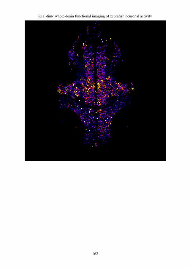
Real-time whole-brain functional imaging of zebrafish neuronal activity
162
163
162

Lapo Turrini
162
163
163

Real-time whole-brain functional imaging of zebrafish neuronal activity
164
165
164

Lapo Turrini
164
165
165

Real-time whole-brain functional imaging of zebrafish neuronal activity
166
167
166
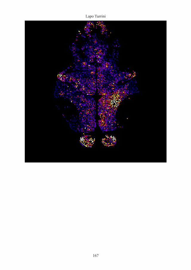
Lapo Turrini
166
167
167

Real-time whole-brain functional imaging of zebrafish neuronal activity
168
169
168

Lapo Turrini
168
169
169

Real-time whole-brain functional imaging of zebrafish neuronal activity
170
171
170

Lapo Turrini
170
171
171

Real-time whole-brain functional imaging of zebrafish neuronal activity
172
173
Figure A3. 2D heat maps used to produce 3D activity maps.
Each of the 23 planes showed were imaged progressively from the dorsal surface of a 4 dpf Tg(elavl3:H2B-GCaMP6s) zebrafish larva. Through a custom Matlab script processing (see Data analysis for details) each neuron identified was expressed with a round symbol having a colour showing its overall activity during the time of measurement (4 minutes) and placed in a virtual image with the original coordinates the neuron had in the original image. Thus, 2D heat maps were produced, expressing the activity of each single neuron present in the imaged plane. Those heat maps were then combined to produce 3D maps of activity showed in Figure 50.
172

Lapo Turrini
172
173
Figure A3. 2D heat maps used to produce 3D activity maps.
Each of the 23 planes showed were imaged progressively from the dorsal surface of a 4 dpf Tg(elavl3:H2B-GCaMP6s) zebrafish larva. Through a custom Matlab script processing (see Data analysis for details) each neuron identified was expressed with a round symbol having a colour showing its overall activity during the time of measurement (4 minutes) and placed in a virtual image with the original coordinates the neuron had in the original image. Thus, 2D heat maps were produced, expressing the activity of each single neuron present in the imaged plane. Those heat maps were then combined to produce 3D maps of activity showed in Figure 50.
173

175
Appendix B Following, the custom Matlab scripts written to perform analysis of 3D mapping of zebrafish neuronal activity by Bessel beam illumination light-sheet fluorescence microscopy.
% The_Cell_Detector.m % % This scripts detect circular-shaped cells or cell nuclei based on local % contrast information. % % Requires Image Processing Toolbox. % % This script only runs on 64-bit Windows because it uses % MEX files build by VS2010. For use in other systems please % re-compile corresponding cpp files. % % % Parameters for cell detection % % outdir -> Output directory of cell recognition result. % fname -> Name of the image file to be analyzed. % br_threshold -> Minimum brightness threshold for the cell to be detected % cont_threshold -> Threshold for local contrast. This sets how the cell % should be brighter than surrounding darkest point. % cell_rad -> Radius of cells to be detected. % % % Output of the script % % cellmask.tif -> Visual result of cell recognition. % cell_info.mat -> Information of detected cells. % [center] y and x coordinate of the detected cell % [area] area of the detected cell % [slice] Z-plane of the detected cell % [inds] one-dimensional indices of the detectec cell % [y_minmax] min and max end of y coordinates % [x_minmax] min and max end of x coordinates % % developed by Francesco Vanzi, European Laboratory for Non-linear % Spectroscopy (LENS), University of Florence, based on a script by Takashi % Kawashima, HHMI Janelia Research Campus (Detailes are described in Kawashima et al., 2016.) % % October 10, 2018 tic clear; MIP=imread('C:\Users\Lapo Turrini\Desktop\Misure
SPIM\zf_12_binned_16bit_registered_ptz_7_5mM\CLAHE(15,256,3)\AVG_Plane24.tif'); MIPmask=imread('C:\Users\Lapo Turrini\Desktop\Misure
SPIM\zf_12_binned_16bit_registered_ptz_7_5mM\CLAHE(15,256,3)mask\AVG_Plane24.tif'); outdir='C:\Users\Lapo Turrini\Desktop\Misure SPIM\zf_12_binned_16bit_registered_ptz_7_5mM\';
%% specify output directory planenumber = 24; % Set the number of the frame you are processing % filename = (['Plane', num2str(planenumber)]); % setting filename with frame number in it % filenamelabel = ([filename,'_celllabel']); br_threshold = 50; % to be set individually for each MIP to be segmented cont_threshold = 8; % to be set accordingly to image contrast (good contrast = 8) cell_rad = 2; % keep it like this, it works just fine %% setting filters and matrices for detecting cells; num_images = 1; dim=[1024 1024 1]; f=[1024 1024]; ave_rad=round(cell_rad/2)+1; [avedisk, ave_se, r1, c1, maskinds]=make_recog_disk(ave_rad,dim); [maxdisk, max_se, r2, c2, maxinds]=make_recog_disk(round(cell_rad*1.5),dim); onedisk=makeDisk(ave_rad,ave_rad*2+1); one_se=strel(onedisk); r=cell_rad*2; dimp=[dim(1)+r*2 dim(2)+r*2]; oop=zeros(dimp);
174

175
Appendix B Following, the custom Matlab scripts written to perform analysis of 3D mapping of zebrafish neuronal activity by Bessel beam illumination light-sheet fluorescence microscopy.
% The_Cell_Detector.m % % This scripts detect circular-shaped cells or cell nuclei based on local % contrast information. % % Requires Image Processing Toolbox. % % This script only runs on 64-bit Windows because it uses % MEX files build by VS2010. For use in other systems please % re-compile corresponding cpp files. % % % Parameters for cell detection % % outdir -> Output directory of cell recognition result. % fname -> Name of the image file to be analyzed. % br_threshold -> Minimum brightness threshold for the cell to be detected % cont_threshold -> Threshold for local contrast. This sets how the cell % should be brighter than surrounding darkest point. % cell_rad -> Radius of cells to be detected. % % % Output of the script % % cellmask.tif -> Visual result of cell recognition. % cell_info.mat -> Information of detected cells. % [center] y and x coordinate of the detected cell % [area] area of the detected cell % [slice] Z-plane of the detected cell % [inds] one-dimensional indices of the detectec cell % [y_minmax] min and max end of y coordinates % [x_minmax] min and max end of x coordinates % % developed by Francesco Vanzi, European Laboratory for Non-linear % Spectroscopy (LENS), University of Florence, based on a script by Takashi % Kawashima, HHMI Janelia Research Campus (Detailes are described in Kawashima et al., 2016.) % % October 10, 2018 tic clear; MIP=imread('C:\Users\Lapo Turrini\Desktop\Misure
SPIM\zf_12_binned_16bit_registered_ptz_7_5mM\CLAHE(15,256,3)\AVG_Plane24.tif'); MIPmask=imread('C:\Users\Lapo Turrini\Desktop\Misure
SPIM\zf_12_binned_16bit_registered_ptz_7_5mM\CLAHE(15,256,3)mask\AVG_Plane24.tif'); outdir='C:\Users\Lapo Turrini\Desktop\Misure SPIM\zf_12_binned_16bit_registered_ptz_7_5mM\';
%% specify output directory planenumber = 24; % Set the number of the frame you are processing % filename = (['Plane', num2str(planenumber)]); % setting filename with frame number in it % filenamelabel = ([filename,'_celllabel']); br_threshold = 50; % to be set individually for each MIP to be segmented cont_threshold = 8; % to be set accordingly to image contrast (good contrast = 8) cell_rad = 2; % keep it like this, it works just fine %% setting filters and matrices for detecting cells; num_images = 1; dim=[1024 1024 1]; f=[1024 1024]; ave_rad=round(cell_rad/2)+1; [avedisk, ave_se, r1, c1, maskinds]=make_recog_disk(ave_rad,dim); [maxdisk, max_se, r2, c2, maxinds]=make_recog_disk(round(cell_rad*1.5),dim); onedisk=makeDisk(ave_rad,ave_rad*2+1); one_se=strel(onedisk); r=cell_rad*2; dimp=[dim(1)+r*2 dim(2)+r*2]; oop=zeros(dimp);
Lapo Turrini, Development of optical methods for real-time whole-brain functional imaging of zebrafish neuronal activity, © 2020 Author(s), content CC BY 4.0 International, metadata CC0 1.0 Universal, published by Firenze University Press (www.fupress.com), ISSN 2612-8020 (online), ISBN 978-88-5518-070-2 (PDF), DOI 10.36253/978-88-5518-070-2

Real-time whole-brain functional imaging of zebrafish neuronal activity
176
oop(r+1:end-r,r+1:end-r)=1; one_inds=find(oop); [mdisk, ~, ~, ~, rankinds]=make_recog_disk(r,dimp); rank_ones=double(maskones2D_mex(int32([dim(1) dim(2)]),int32(mdisk),int32(size(mdisk))))'; %% detecting cells mkdir(outdir); cell_info=struct; cell_color=zeros([dim(1) dim(2)*2+1 dim(3) 3],'uint8'); cellnum=0; allmask=zeros(dim(1),dim(2)); imlen=dim(1)*dim(2); for z=1:dim(3) im=MIPmask; allmask(:)=0; contimage = local_contrast_mex(single(im),int32(32),single(cont_threshold)); figure imagesc(contimage, [0 1]) contimage = imdilate(imerode(contimage,one_se),one_se); contimage = contimage.*uint8((im>br_threshold)); candidates=find(contimage); if ~isempty(candidates) %% recognizing cells in the first round imrank = calc_local_rank(im,rank_ones,cell_rad*2,oop,one_inds,rankinds,candidates); aveimg =
double(local_average_mex(single(imrank),int32(c1),int32(r1),int32(candidates))); maximg = double(local_max_mex(single(aveimg),int32(c2),int32(r2),int32(candidates))); inds=find(maximg(candidates)>0 & aveimg(candidates) >0.4); mask2=zeros(dim(1),dim(2)); for i=1:length(inds) cinds=candidates(inds(i))+maskinds; cinds(cinds > imlen | cinds<1)=[]; mask2(cinds)=1; end allmask=mask2; %% recognizing cells in the second round mask3=ones(size(im),'uint8')-imdilate(uint8(allmask),max_se); mask3 = imdilate(imerode(mask3,one_se),one_se); candidates2=candidates(mask3(candidates)>0); imrank2 = calc_local_rank(im,rank_ones,cell_rad*2,oop,one_inds,rankinds,candidates2); aveimg2 =
double(local_average_mex(single(imrank2),int32(c1),int32(r1),int32(candidates2))); maximg2 =
double(local_max_mex(single(aveimg2),int32(c1),int32(r1),int32(candidates2))); inds=find(maximg2(candidates2)>0 & aveimg2(candidates2) >0.4); mask2=zeros(dim(1),dim(2)); for i=1:length(inds) cinds=candidates2(inds(i))+maskinds; cinds(cinds > imlen | cinds<1)=[]; mask2(cinds)=1; end allmask=allmask+mask2; % fv cellkernel=[0 0 1 0 0;0 1 1 1 0;1 1 1 1 1;0 1 1 1 0;0 0 1 0 0]; % fv FVCell=deconvlucy(allmask,cellkernel); % fv FVCell=ceil(FVCell.*(FVCell>0.8)); % fv %% create each cell ROIs % The following four commands represent the difference between Kawashima et al, 2016. % method
and ours. Use first line and comment second to fourth to use Kawashima. % Comment only first line to use ours. %[celllabel, totcell]=bwlabel(allmask,8); [celllabel, totcell]=bwlabel(FVCell); celllabel=conv2(celllabel,cellkernel); celllabel=celllabel(3:1026,3:1026);
177
if totcell>0 cell_info=create_cell_info(cell_info,celllabel, totcell,z); end else totcell=0; celllabel=zeros(size(im)); end cell_color(:,:,z,:)=reshape(make2DMask(MIP,celllabel,candidates),[dim(1) dim(2)*2+1 1 3]); cellnum=cellnum+totcell; disp(num2str(z)); end %% Saving files write_colortiff_mex(fullfile(outdir, 'Plane24.tif'),cell_color, int32(size(cell_color))); save(fullfile(outdir, 'Plane24.mat'),'cell_info'); save(fullfile(outdir, 'Plane24_celllabel.mat'),'celllabel'); toc
% The_DF_F_calculator.m % % This scripts calculate DF/F0 from large stacks using coordinates data produced by
The_Cell_detector.m % % Requires Image Processing Toolbox. % % % Parameters for cell detection % % % % Output of the script % % % developed by Francesco Vanzi and Lapo Turrini, European Laboratory for Non-linear % Spectroscopy (LENS), University of Florence % % October 10, 2018 %% Loading.tif stack tic clear; % Loading cell info file load('C:\Users\Lapo Turrini\Desktop\Misure
SPIM\zf_12_binned_16bit_registered_ptz_7_5mM\Results\24\Plane24.mat'); load('C:\Users\Lapo Turrini\Desktop\Misure
SPIM\zf_12_binned_16bit_registered_ptz_7_5mM\Results\24\Plane24_celllabel.mat'); outdir = 'C:\Users\Lapo Turrini\Desktop\Misure
SPIM\zf_12_binned_16bit_registered_ptz_7_5mM\Results\24\'; %% specify output directory FileTif = 'C:\Users\Lapo Turrini\Desktop\Misure
SPIM\zf_12_binned_16bit_registered_ptz_7_5mM\Downsampled, Binned, Registered\Plane24.tif'; InfoImage = imfinfo(FileTif); mImage = InfoImage(1).Width; nImage = InfoImage(1).Height; NumberImages = length(InfoImage); FinalImage = zeros(nImage,mImage,NumberImages,'uint16'); % use 'uint8' for 8-bit images or
'uint16' for 16-bit images f=[mImage nImage]; % Number of pixels for each side of the FOV totcell = length(cell_info); % Total number of cells detected TifLink = Tiff(FileTif, 'r'); for i = 1:NumberImages TifLink.setDirectory(i); FinalImage(:,:,i) = TifLink.read(); end TifLink.close(); %% Extracting DF/F from stack using segmentation x,y coordinates
176

Lapo Turrini
176
oop(r+1:end-r,r+1:end-r)=1; one_inds=find(oop); [mdisk, ~, ~, ~, rankinds]=make_recog_disk(r,dimp); rank_ones=double(maskones2D_mex(int32([dim(1) dim(2)]),int32(mdisk),int32(size(mdisk))))'; %% detecting cells mkdir(outdir); cell_info=struct; cell_color=zeros([dim(1) dim(2)*2+1 dim(3) 3],'uint8'); cellnum=0; allmask=zeros(dim(1),dim(2)); imlen=dim(1)*dim(2); for z=1:dim(3) im=MIPmask; allmask(:)=0; contimage = local_contrast_mex(single(im),int32(32),single(cont_threshold)); figure imagesc(contimage, [0 1]) contimage = imdilate(imerode(contimage,one_se),one_se); contimage = contimage.*uint8((im>br_threshold)); candidates=find(contimage); if ~isempty(candidates) %% recognizing cells in the first round imrank = calc_local_rank(im,rank_ones,cell_rad*2,oop,one_inds,rankinds,candidates); aveimg =
double(local_average_mex(single(imrank),int32(c1),int32(r1),int32(candidates))); maximg = double(local_max_mex(single(aveimg),int32(c2),int32(r2),int32(candidates))); inds=find(maximg(candidates)>0 & aveimg(candidates) >0.4); mask2=zeros(dim(1),dim(2)); for i=1:length(inds) cinds=candidates(inds(i))+maskinds; cinds(cinds > imlen | cinds<1)=[]; mask2(cinds)=1; end allmask=mask2; %% recognizing cells in the second round mask3=ones(size(im),'uint8')-imdilate(uint8(allmask),max_se); mask3 = imdilate(imerode(mask3,one_se),one_se); candidates2=candidates(mask3(candidates)>0); imrank2 = calc_local_rank(im,rank_ones,cell_rad*2,oop,one_inds,rankinds,candidates2); aveimg2 =
double(local_average_mex(single(imrank2),int32(c1),int32(r1),int32(candidates2))); maximg2 =
double(local_max_mex(single(aveimg2),int32(c1),int32(r1),int32(candidates2))); inds=find(maximg2(candidates2)>0 & aveimg2(candidates2) >0.4); mask2=zeros(dim(1),dim(2)); for i=1:length(inds) cinds=candidates2(inds(i))+maskinds; cinds(cinds > imlen | cinds<1)=[]; mask2(cinds)=1; end allmask=allmask+mask2; % fv cellkernel=[0 0 1 0 0;0 1 1 1 0;1 1 1 1 1;0 1 1 1 0;0 0 1 0 0]; % fv FVCell=deconvlucy(allmask,cellkernel); % fv FVCell=ceil(FVCell.*(FVCell>0.8)); % fv %% create each cell ROIs % The following four commands represent the difference between Kawashima et al, 2016. % method
and ours. Use first line and comment second to fourth to use Kawashima. % Comment only first line to use ours. %[celllabel, totcell]=bwlabel(allmask,8); [celllabel, totcell]=bwlabel(FVCell); celllabel=conv2(celllabel,cellkernel); celllabel=celllabel(3:1026,3:1026);
177
if totcell>0 cell_info=create_cell_info(cell_info,celllabel, totcell,z); end else totcell=0; celllabel=zeros(size(im)); end cell_color(:,:,z,:)=reshape(make2DMask(MIP,celllabel,candidates),[dim(1) dim(2)*2+1 1 3]); cellnum=cellnum+totcell; disp(num2str(z)); end %% Saving files write_colortiff_mex(fullfile(outdir, 'Plane24.tif'),cell_color, int32(size(cell_color))); save(fullfile(outdir, 'Plane24.mat'),'cell_info'); save(fullfile(outdir, 'Plane24_celllabel.mat'),'celllabel'); toc
% The_DF_F_calculator.m % % This scripts calculate DF/F0 from large stacks using coordinates data produced by
The_Cell_detector.m % % Requires Image Processing Toolbox. % % % Parameters for cell detection % % % % Output of the script % % % developed by Francesco Vanzi and Lapo Turrini, European Laboratory for Non-linear % Spectroscopy (LENS), University of Florence % % October 10, 2018 %% Loading.tif stack tic clear; % Loading cell info file load('C:\Users\Lapo Turrini\Desktop\Misure
SPIM\zf_12_binned_16bit_registered_ptz_7_5mM\Results\24\Plane24.mat'); load('C:\Users\Lapo Turrini\Desktop\Misure
SPIM\zf_12_binned_16bit_registered_ptz_7_5mM\Results\24\Plane24_celllabel.mat'); outdir = 'C:\Users\Lapo Turrini\Desktop\Misure
SPIM\zf_12_binned_16bit_registered_ptz_7_5mM\Results\24\'; %% specify output directory FileTif = 'C:\Users\Lapo Turrini\Desktop\Misure
SPIM\zf_12_binned_16bit_registered_ptz_7_5mM\Downsampled, Binned, Registered\Plane24.tif'; InfoImage = imfinfo(FileTif); mImage = InfoImage(1).Width; nImage = InfoImage(1).Height; NumberImages = length(InfoImage); FinalImage = zeros(nImage,mImage,NumberImages,'uint16'); % use 'uint8' for 8-bit images or
'uint16' for 16-bit images f=[mImage nImage]; % Number of pixels for each side of the FOV totcell = length(cell_info); % Total number of cells detected TifLink = Tiff(FileTif, 'r'); for i = 1:NumberImages TifLink.setDirectory(i); FinalImage(:,:,i) = TifLink.read(); end TifLink.close(); %% Extracting DF/F from stack using segmentation x,y coordinates
177

Real-time whole-brain functional imaging of zebrafish neuronal activity
178
FrameRate = 5; % Actual frame-rate of the loaded stack expressed in Hz fr = (1:NumberImages)'; tr = zeros(NumberImages,totcell); DF_F = zeros(NumberImages,totcell); for cn = 1:totcell [x,y] = ind2sub(f,find(celllabel==cn)); SInt = double(0); for coordpair = 1:length(x) SInt = double(double(SInt)+double(FinalImage(x(coordpair),y(coordpair),:)));
%FinalImage is the image stack: x,y,t matrix end trt = squeeze(SInt); if cn == 1 tr = double(trt); else tr = [tr double(trt)]; end DF = msbackadj(fr,trt,'WindowSize',50,'StepSize',10,'SmoothMethod','lowess'); F0 = trt-DF; MF0 = min(F0); if MF0>15 DF_F_temp = DF./F0; else DF_F_temp(fr) = 0; end DF_F(fr,cn) = DF_F_temp(fr); end save(fullfile(outdir, 'DF_F24.mat'),'DF_F'); toc
% The_Peaks_Finder.m % % This scripts identifies peaks of fluorescence activity in DF/F0 traces produced by % The_DF_F_Calculator.m and produces a heat-map attributing activity to each single cell
detected by The_Cell_Detector.m % % Requires Image Processing Toolbox. % % % Parameters for cell detection % % % % Output of the script % % % developed by Lapo Turrini, European Laboratory for Non-linear Spectroscopy (LENS),
University of Florence % % October 10, 2018 tic clear; %% Loading DF/F file load('C:\Users\Lapo Turrini\Desktop\Misure
SPIM\zf_12_binned_16bit_registered_ptz_7_5mM\Results\24\DF_F24.mat') %% Loading cell info file load('C:\Users\Lapo Turrini\Desktop\Misure
SPIM\zf_12_binned_16bit_registered_ptz_7_5mM\Results\24\Plane24.mat') %% Loading MIP file MIP = imread('C:\Users\Lapo Turrini\Desktop\Misure
SPIM\zf_12_binned_16bit_registered_ptz_7_5mM\CLAHE(15,256,3)\AVG_Plane24.tif'); % Setting output directory outdir='C:\Users\Lapo Turrini\Desktop\Misure
SPIM\zf_12_binned_16bit_registered_ptz_7_5mM\Results\activity map\'; %% specify output directory planenumber = 24; % Set the number of the frame you are processing
179
filename_sum_pks = (['SUMpeak_', num2str(planenumber)]); filename_sum_p = (['SUMprominence_', num2str(planenumber)]); % setting filename with frame
number dim = [1024 1024 1]; % Image size in pixel F = length(DF_F(:,1)); % number of frames C = length(DF_F(1,:)); % total number of cells order = 3; framelen = 17; FR = 5; % Actual framerate considering downsample iftbr = 50; % Initial frames to be removed %% Removing initial frames for k = 1:C DF_Fclean(:,k) = DF_F(iftbr:end,k); end Fclean = length(DF_Fclean(:,1)); % number of clean frames %% Allocating memory smoothedDF_F = zeros(Fclean,C); P{C} = []; sum_pks = zeros(1,C); sum_p = zeros(1,C); sum_p_mask = zeros(dim(1),dim(2)); sum_pks_mask = zeros(dim(1),dim(2)); %% Converting number of frames in time n_frames = (1:Fclean)'; % all frames time = n_frames*(1/FR); % number of frames converted in time [s] meas_length = time(end); % time of measurement %% Applying Savitzky-Golay smoothing to each DF/F trace for i = 1 : C smoothedDF_F(:,i) = sgolayfilt(DF_Fclean(:,i),order, framelen); end %% Performing findpeaks on each smoothed DF/F trace for j = 1 : C [pks,locs,w,p] =
findpeaks(smoothedDF_F(:,j),'MinPeakProminence',0.02,'Annotate','extents'); P{j} = [pks,locs,w,p]; end %% Calculating sum of both peak maximum and peak amplitude for k = 1 : C sum_pks(:,k) = sum(P{1,k}(:,1)); % calculating sum of the first column (pks) for each
trace sum_p(:,k) = std(P{1,k}(:,4)); % calculating sum of the fourth column (p) for each trace end %% Extracting cell coordinates center = {cell_info.center}.'; center_coordinates = cell2mat(center); x_center = center_coordinates(:,2); y_center = center_coordinates(:,1); % cellkernel = [0 0 1 0 0;0 1 1 1 0;1 1 1 1 1;0 1 1 1 0;0 0 1 0 0]; % squarish cells cellkernel = [0 0 0 1 0 0 0;0 1 1 1 1 1 0;0 1 1 1 1 1 0;1 1 1 1 1 1 1;0 1 1 1 1 1 0;0 1 1 1 1
1 0;0 0 0 1 0 0 0]; % round cells %% Creating a mask with each cell showing the sum of its peak's amplitude (prominence) for i = 1:C sum_p_mask(x_center(i),y_center(i)) = sum_p(:,i); end % sum_p_mask = sum_p_mask./meas_length; sum_p_mask = (sum_p_mask)';
178

Lapo Turrini
178
FrameRate = 5; % Actual frame-rate of the loaded stack expressed in Hz fr = (1:NumberImages)'; tr = zeros(NumberImages,totcell); DF_F = zeros(NumberImages,totcell); for cn = 1:totcell [x,y] = ind2sub(f,find(celllabel==cn)); SInt = double(0); for coordpair = 1:length(x) SInt = double(double(SInt)+double(FinalImage(x(coordpair),y(coordpair),:)));
%FinalImage is the image stack: x,y,t matrix end trt = squeeze(SInt); if cn == 1 tr = double(trt); else tr = [tr double(trt)]; end DF = msbackadj(fr,trt,'WindowSize',50,'StepSize',10,'SmoothMethod','lowess'); F0 = trt-DF; MF0 = min(F0); if MF0>15 DF_F_temp = DF./F0; else DF_F_temp(fr) = 0; end DF_F(fr,cn) = DF_F_temp(fr); end save(fullfile(outdir, 'DF_F24.mat'),'DF_F'); toc
% The_Peaks_Finder.m % % This scripts identifies peaks of fluorescence activity in DF/F0 traces produced by % The_DF_F_Calculator.m and produces a heat-map attributing activity to each single cell
detected by The_Cell_Detector.m % % Requires Image Processing Toolbox. % % % Parameters for cell detection % % % % Output of the script % % % developed by Lapo Turrini, European Laboratory for Non-linear Spectroscopy (LENS),
University of Florence % % October 10, 2018 tic clear; %% Loading DF/F file load('C:\Users\Lapo Turrini\Desktop\Misure
SPIM\zf_12_binned_16bit_registered_ptz_7_5mM\Results\24\DF_F24.mat') %% Loading cell info file load('C:\Users\Lapo Turrini\Desktop\Misure
SPIM\zf_12_binned_16bit_registered_ptz_7_5mM\Results\24\Plane24.mat') %% Loading MIP file MIP = imread('C:\Users\Lapo Turrini\Desktop\Misure
SPIM\zf_12_binned_16bit_registered_ptz_7_5mM\CLAHE(15,256,3)\AVG_Plane24.tif'); % Setting output directory outdir='C:\Users\Lapo Turrini\Desktop\Misure
SPIM\zf_12_binned_16bit_registered_ptz_7_5mM\Results\activity map\'; %% specify output directory planenumber = 24; % Set the number of the frame you are processing
179
filename_sum_pks = (['SUMpeak_', num2str(planenumber)]); filename_sum_p = (['SUMprominence_', num2str(planenumber)]); % setting filename with frame
number dim = [1024 1024 1]; % Image size in pixel F = length(DF_F(:,1)); % number of frames C = length(DF_F(1,:)); % total number of cells order = 3; framelen = 17; FR = 5; % Actual framerate considering downsample iftbr = 50; % Initial frames to be removed %% Removing initial frames for k = 1:C DF_Fclean(:,k) = DF_F(iftbr:end,k); end Fclean = length(DF_Fclean(:,1)); % number of clean frames %% Allocating memory smoothedDF_F = zeros(Fclean,C); P{C} = []; sum_pks = zeros(1,C); sum_p = zeros(1,C); sum_p_mask = zeros(dim(1),dim(2)); sum_pks_mask = zeros(dim(1),dim(2)); %% Converting number of frames in time n_frames = (1:Fclean)'; % all frames time = n_frames*(1/FR); % number of frames converted in time [s] meas_length = time(end); % time of measurement %% Applying Savitzky-Golay smoothing to each DF/F trace for i = 1 : C smoothedDF_F(:,i) = sgolayfilt(DF_Fclean(:,i),order, framelen); end %% Performing findpeaks on each smoothed DF/F trace for j = 1 : C [pks,locs,w,p] =
findpeaks(smoothedDF_F(:,j),'MinPeakProminence',0.02,'Annotate','extents'); P{j} = [pks,locs,w,p]; end %% Calculating sum of both peak maximum and peak amplitude for k = 1 : C sum_pks(:,k) = sum(P{1,k}(:,1)); % calculating sum of the first column (pks) for each
trace sum_p(:,k) = std(P{1,k}(:,4)); % calculating sum of the fourth column (p) for each trace end %% Extracting cell coordinates center = {cell_info.center}.'; center_coordinates = cell2mat(center); x_center = center_coordinates(:,2); y_center = center_coordinates(:,1); % cellkernel = [0 0 1 0 0;0 1 1 1 0;1 1 1 1 1;0 1 1 1 0;0 0 1 0 0]; % squarish cells cellkernel = [0 0 0 1 0 0 0;0 1 1 1 1 1 0;0 1 1 1 1 1 0;1 1 1 1 1 1 1;0 1 1 1 1 1 0;0 1 1 1 1
1 0;0 0 0 1 0 0 0]; % round cells %% Creating a mask with each cell showing the sum of its peak's amplitude (prominence) for i = 1:C sum_p_mask(x_center(i),y_center(i)) = sum_p(:,i); end % sum_p_mask = sum_p_mask./meas_length; sum_p_mask = (sum_p_mask)';
179

Real-time whole-brain functional imaging of zebrafish neuronal activity
180
fnan_p = find(isnan(sum_p_mask)); % find NaN in sum_prominence mask sum_p_mask(fnan_p) = 0; % setting at 0 all found NaN sum_p_map = imdilate (sum_p_mask,cellkernel); imwrite(sum_p_map,fullfile(outdir, filename_sum_p), 'tif'); dlmwrite(filename_sum_p,sum_p_map); %% Generating a mask with each cell showing the sum of its peak's maxima for i = 1:C sum_pks_mask(x_center(i),y_center(i)) = sum_pks(:,i); end sum_pks_mask = sum_pks_mask./meas_length; sum_pks_mask = (sum_pks_mask)'; fnan_pks = find(isnan(sum_pks_mask)); % find NaN in sum_pks mask sum_pks_mask(fnan_pks) = 0; % setting at 0 all found NaN sum_pks_map = imdilate(sum_pks_mask,cellkernel); imwrite(sum_pks_map,fullfile(outdir, filename_sum_pks),'tif'); dlmwrite(filename_sum_pks,sum_pks_map); toc
181
Bibliography
Abraham, E., Palevitch, O., Gothilf, Y., and Zohar, Y. (2009). The zebrafish as a model system for forebrain GnRH neuronal development. Gen Comp Endocrinol 164, 151-160.
Afrikanova, T., Serruys, A.S., Buenafe, O.E., Clinckers, R., Smolders, I., De Witte, P.A., Crawford, A.D., and Esguerra, C.V. (2013). Validation of the zebrafish pentylenetetrazol seizure model: locomotor versus electrographic responses to antiepileptic drugs. PLoS One 8, e54166.
Ahrens, M.B., Orger, M.B., Robson, D.N., Li, J.M., and Keller, P.J. (2013). Whole-brain functional imaging at cellular resolution using light-sheet microscopy. Nat Methods 10, 413-420.
Akerboom, J., Chen, T.W., Wardill, T.J., Tian, L., Marvin, J.S., Mutlu, S., Calderon, N.C., Esposti, F., Borghuis, B.G., Sun, X.R., Gordus, A., Orger, M.B., Portugues, R., Engert, F., Macklin, J.J., Filosa, A., Aggarwal, A., Kerr, R.A., Takagi, R., Kracun, S., Shigetomi, E., Khakh, B.S., Baier, H., Lagnado, L., Wang, S.S., Bargmann, C.I., Kimmel, B.E., Jayaraman, V., Svoboda, K., Kim, D.S., Schreiter, E.R., and Looger, L.L. (2012). Optimization of a GCaMP calcium indicator for neural activity imaging. J Neurosci 32, 13819-13840.
Akerboom, J., Rivera, J.D., Guilbe, M.M., Malave, E.C., Hernandez, H.H., Tian, L., Hires, S.A., Marvin, J.S., Looger, L.L., and Schreiter, E.R. (2009). Crystal structures of the GCaMP calcium sensor reveal the mechanism of fluorescence signal change and aid rational design. J Biol Chem 284, 6455-6464.
Allegra Mascaro, A.L., Conti, E., Lai, S., Di Giovanna, A.P., Spalletti, C., Alia, C., Panarese, A., Scaglione, A., Sacconi, L., Micera, S., Caleo, M., and Pavone, F.S. (2019). Combined Rehabilitation Promotes the Recovery of Structural and Functional Features of Healthy Neuronal Networks after Stroke. Cell Rep 28, 3474-3485 e3476.
Attili, S., and Hughes, S.M. (2014). Anaesthetic tricaine acts preferentially on neural voltage-gated sodium channels and fails to block directly evoked muscle contraction. PLoS One 9, e103751.
Attwell, D., Buchan, A.M., Charpak, S., Lauritzen, M., Macvicar, B.A., and Newman, E.A. (2010). Glial and neuronal control of brain blood flow. Nature 468, 232-243.
Azevedo, F.A., Carvalho, L.R., Grinberg, L.T., Farfel, J.M., Ferretti, R.E., Leite, R.E., Jacob Filho, W., Lent, R., and Herculano-Houzel, S. (2009). Equal numbers of neuronal and nonneuronal cells make the human brain an isometrically scaled-up primate brain. J Comp Neurol 513, 532-541.
Baird, G.S., Zacharias, D.A., and Tsien, R.Y. (1999). Circular permutation and receptor insertion within green fluorescent proteins. Proc Natl Acad Sci U S A 96, 11241-11246.
Baker, P.F., Hodgkin, A.L., and Ridgway, E.B. (1971). Depolarization and calcium entry in squid giant axons. J Physiol 218, 709-755.
Baraban, S.C., Dinday, M.T., and Hortopan, G.A. (2013). Drug screening in Scn1a zebrafish mutant identifies clemizole as a potential Dravet syndrome treatment. Nat Commun 4, 2410.
180

180
fnan_p = find(isnan(sum_p_mask)); % find NaN in sum_prominence mask sum_p_mask(fnan_p) = 0; % setting at 0 all found NaN sum_p_map = imdilate (sum_p_mask,cellkernel); imwrite(sum_p_map,fullfile(outdir, filename_sum_p), 'tif'); dlmwrite(filename_sum_p,sum_p_map); %% Generating a mask with each cell showing the sum of its peak's maxima for i = 1:C sum_pks_mask(x_center(i),y_center(i)) = sum_pks(:,i); end sum_pks_mask = sum_pks_mask./meas_length; sum_pks_mask = (sum_pks_mask)'; fnan_pks = find(isnan(sum_pks_mask)); % find NaN in sum_pks mask sum_pks_mask(fnan_pks) = 0; % setting at 0 all found NaN sum_pks_map = imdilate(sum_pks_mask,cellkernel); imwrite(sum_pks_map,fullfile(outdir, filename_sum_pks),'tif'); dlmwrite(filename_sum_pks,sum_pks_map); toc
181
Bibliography
Abraham, E., Palevitch, O., Gothilf, Y., and Zohar, Y. (2009). The zebrafish as a model system for forebrain GnRH neuronal development. Gen Comp Endocrinol 164, 151-160.
Afrikanova, T., Serruys, A.S., Buenafe, O.E., Clinckers, R., Smolders, I., De Witte, P.A., Crawford, A.D., and Esguerra, C.V. (2013). Validation of the zebrafish pentylenetetrazol seizure model: locomotor versus electrographic responses to antiepileptic drugs. PLoS One 8, e54166.
Ahrens, M.B., Orger, M.B., Robson, D.N., Li, J.M., and Keller, P.J. (2013). Whole-brain functional imaging at cellular resolution using light-sheet microscopy. Nat Methods 10, 413-420.
Akerboom, J., Chen, T.W., Wardill, T.J., Tian, L., Marvin, J.S., Mutlu, S., Calderon, N.C., Esposti, F., Borghuis, B.G., Sun, X.R., Gordus, A., Orger, M.B., Portugues, R., Engert, F., Macklin, J.J., Filosa, A., Aggarwal, A., Kerr, R.A., Takagi, R., Kracun, S., Shigetomi, E., Khakh, B.S., Baier, H., Lagnado, L., Wang, S.S., Bargmann, C.I., Kimmel, B.E., Jayaraman, V., Svoboda, K., Kim, D.S., Schreiter, E.R., and Looger, L.L. (2012). Optimization of a GCaMP calcium indicator for neural activity imaging. J Neurosci 32, 13819-13840.
Akerboom, J., Rivera, J.D., Guilbe, M.M., Malave, E.C., Hernandez, H.H., Tian, L., Hires, S.A., Marvin, J.S., Looger, L.L., and Schreiter, E.R. (2009). Crystal structures of the GCaMP calcium sensor reveal the mechanism of fluorescence signal change and aid rational design. J Biol Chem 284, 6455-6464.
Allegra Mascaro, A.L., Conti, E., Lai, S., Di Giovanna, A.P., Spalletti, C., Alia, C., Panarese, A., Scaglione, A., Sacconi, L., Micera, S., Caleo, M., and Pavone, F.S. (2019). Combined Rehabilitation Promotes the Recovery of Structural and Functional Features of Healthy Neuronal Networks after Stroke. Cell Rep 28, 3474-3485 e3476.
Attili, S., and Hughes, S.M. (2014). Anaesthetic tricaine acts preferentially on neural voltage-gated sodium channels and fails to block directly evoked muscle contraction. PLoS One 9, e103751.
Attwell, D., Buchan, A.M., Charpak, S., Lauritzen, M., Macvicar, B.A., and Newman, E.A. (2010). Glial and neuronal control of brain blood flow. Nature 468, 232-243.
Azevedo, F.A., Carvalho, L.R., Grinberg, L.T., Farfel, J.M., Ferretti, R.E., Leite, R.E., Jacob Filho, W., Lent, R., and Herculano-Houzel, S. (2009). Equal numbers of neuronal and nonneuronal cells make the human brain an isometrically scaled-up primate brain. J Comp Neurol 513, 532-541.
Baird, G.S., Zacharias, D.A., and Tsien, R.Y. (1999). Circular permutation and receptor insertion within green fluorescent proteins. Proc Natl Acad Sci U S A 96, 11241-11246.
Baker, P.F., Hodgkin, A.L., and Ridgway, E.B. (1971). Depolarization and calcium entry in squid giant axons. J Physiol 218, 709-755.
Baraban, S.C., Dinday, M.T., and Hortopan, G.A. (2013). Drug screening in Scn1a zebrafish mutant identifies clemizole as a potential Dravet syndrome treatment. Nat Commun 4, 2410.
Lapo Turrini, Development of optical methods for real-time whole-brain functional imaging of zebrafish neuronal activity, © 2020 Author(s), content CC BY 4.0 International, metadata CC0 1.0 Universal, published by Firenze University Press (www.fupress.com), ISSN 2612-8020 (online), ISBN 978-88-5518-070-2 (PDF), DOI 10.36253/978-88-5518-070-2

Real-time whole-brain functional imaging of zebrafish neuronal activity
182
Baraban, S.C., Taylor, M.R., Castro, P.A., and Baier, H. (2005). Pentylenetetrazole induced changes in zebrafish behavior, neural activity and c-fos expression. Neuroscience 131, 759-768.
Barbazuk, W.B., Korf, I., Kadavi, C., Heyen, J., Tate, S., Wun, E., Bedell, J.A., Mcpherson, J.D., and Johnson, S.L. (2000). The syntenic relationship of the zebrafish and human genomes. Genome Res 10, 1351-1358.
Bargmann, C.I. (1998). Neurobiology of the Caenorhabditis elegans genome. Science 282, 2028-2033.
Baumgart, E., and Kubitscheck, U. (2012). Scanned light sheet microscopy with confocal slit detection. Opt Express 20, 21805-21814.
Baxendale, S., Holdsworth, C.J., Meza Santoscoy, P.L., Harrison, M.R., Fox, J., Parkin, C.A., Ingham, P.W., and Cunliffe, V.T. (2012). Identification of compounds with anti-convulsant properties in a zebrafish model of epileptic seizures. Dis Model Mech 5, 773-784.
Blader, P., and Strahle, U. (2000). Zebrafish developmental genetics and central nervous system development. Hum Mol Genet 9, 945-951.
Burgess, N., and O'keefe, J. (2003). Neural representations in human spatial memory. Trends Cogn Sci 7, 517-519.
Candelier, R., Murmu, M.S., Romano, S.A., Jouary, A., Debregeas, G., and Sumbre, G. (2015). A microfluidic device to study neuronal and motor responses to acute chemical stimuli in zebrafish. Sci Rep 5, 12196.
Chaigneau, E., Ronzitti, E., Gajowa, M.A., Soler-Llavina, G.J., Tanese, D., Brureau, A.Y., Papagiakoumou, E., Zeng, H., and Emiliani, V. (2016). Two-Photon Holographic Stimulation of ReaChR. Front Cell Neurosci 10, 234.
Chalfie, M., Tu, Y., Euskirchen, G., Ward, W.W., and Prasher, D.C. (1994). Green fluorescent protein as a marker for gene expression. Science 263, 802-805.
Chattoraj, M., King, B.A., Bublitz, G.U., and Boxer, S.G. (1996). Ultra-fast excited state dynamics in green fluorescent protein: multiple states and proton transfer. Proc Natl Acad Sci U S A 93, 8362-8367.
Chen, B.R., Kozberg, M.G., Bouchard, M.B., Shaik, M.A., and Hillman, E.M. (2014). A critical role for the vascular endothelium in functional neurovascular coupling in the brain. J Am Heart Assoc 3, e000787.
Chen, T.W., Wardill, T.J., Sun, Y., Pulver, S.R., Renninger, S.L., Baohan, A., Schreiter, E.R., Kerr, R.A., Orger, M.B., Jayaraman, V., Looger, L.L., Svoboda, K., and Kim, D.S. (2013). Ultrasensitive fluorescent proteins for imaging neuronal activity. Nature 499, 295-300.
Chen, Y., Glaser, A., and Liu, J.T. (2017). Bessel-beam illumination in dual-axis confocal microscopy mitigates resolution degradation caused by refractive heterogeneities. J Biophotonics 10, 68-74.
Chhabria, K., Plant, K., Bandmann, O., Wilkinson, R., Martin, C., Kugler, E., Armitage, P., Santoscoy, P., Cunliffe, V.T., Huisken, J., Mcgown, A., Ramesh, R., Chico, T., and Howarth, C. (2018). The effect of Hyperglycemia on neurovascular coupling and cerebrovascular patterning in zebrafish. Journal of Cerebral Blood Flow and Metabolism.
Chitalia, R., Mueller, J., Fu, H.L., Whitley, M.J., Kirsch, D.G., Brown, J.Q., Willett, R., and Ramanujam, N. (2016). Algorithms for differentiating between images of heterogeneous tissue across fluorescence microscopes. Biomed Opt Express 7, 3412-3424.
Cho, S.J., Byun, D., Nam, T.S., Choi, S.Y., Lee, B.G., Kim, M.K., and Kim, S. (2017). Zebrafish as an animal model in epilepsy studies with multichannel EEG recordings. Sci Rep 7, 3099.
Cong, L., Wang, Z., Chai, Y., Hang, W., Shang, C., Yang, W., Bai, L., Du, J., Wang, K., and Wen, Q. (2017). Rapid whole brain imaging of neural activity in freely behaving larval zebrafish (Danio rerio). Elife 6.
183
Conti, E., Allegra Mascaro, A.L., and Pavone, F.S. (2019). Large Scale Double-Path Illumination System with Split Field of View for the All-Optical Study of Inter-and Intra-Hemispheric Functional Connectivity on Mice. Methods Protoc 2.
Craggs, T.D. (2009). Green fluorescent protein: structure, folding and chromophore maturation. Chem Soc Rev 38, 2865-2875.
Creaser C.W. (1934). The technique of handling the zebrafish (Brachydanio rerio) for the production of eggs which are favourable for embryological research and are available at any specified time throughout the year. Copeia, 159-161.
Crocini, C., Ferrantini, C., Coppini, R., Scardigli, M., Yan, P., Loew, L.M., Smith, G., Cerbai, E., Poggesi, C., Pavone, F.S., and Sacconi, L. (2016). Optogenetics design of mechanistically-based stimulation patterns for cardiac defibrillation. Sci Rep 6, 35628.
Cubitt, A.B., Heim, R., Adams, S.R., Boyd, A.E., Gross, L.A., and Tsien, R.Y. (1995). Understanding, improving and using green fluorescent proteins. Trends Biochem Sci 20, 448-455.
Dekens, M.P., Foulkes, N.S., and Tessmar-Raible, K. (2017). Instrument design and protocol for the study of light controlled processes in aquatic organisms, and its application to examine the effect of infrared light on zebrafish. PLoS One 12, e0172038.
Denk, W., Strickler, J.H., and Webb, W.W. (1990). Two-photon laser scanning fluorescence microscopy. Science 248, 73-76.
de Vito, G., Turrini, L., Fornetto, C., Ricci, P., Müllenbroich, M.C., Sancataldo, G., Trabalzini, E., Mazzamuto, G., Tiso, N., Fanelli, D., Silvestri, L., Vanzi, F., Pavone, F.S. (2020). Application of two-photon light-sheet microscopy to high-speed whole-brain functional imaging of zebrafish neuronal physiology and pathology. Photonics Europe 2020 SPIE. SPIE Photonics Europe, doi: doi.org/10.1117/12.2560341.
de Vito, G., Ricci, P., Turrini, L., Tiso, N., Vanzi, F., Silvestri, L., Pavone, F.S. (2020). Effects of excitation light polarization on fluorescence emission in two-photon light-sheet microscopy. arXiv:2003.09496 pre-print.
de Vito, G., Fornetto, C., Ricci, P., Müllenbroich, M.C., Sancataldo, G., Turrini, L., Mazzamuto, G., Tiso, N., Sacconi, L., Fanelli, D., Silvestri, L., Vanzi, F., Pavone, F.S. (2020). Two-photon high-speed light-sheet volumetric imaging of brain activity during sleep in zebrafish larvae, Photonics West 2020 BiOS. SPIE BiOS, doi: doi.org/10.1117/12.2542285.
Dinday, M.T., and Baraban, S.C. (2015). Large-Scale Phenotype-Based Antiepileptic Drug Screening in a Zebrafish Model of Dravet Syndrome. eNeuro 2.
Dombeck, D.A., Harvey, C.D., Tian, L., Looger, L.L., and Tank, D.W. (2010). Functional imaging of hippocampal place cells at cellular resolution during virtual navigation. Nat Neurosci 13, 1433-1440.
Duchen, M.R. (1999). Contributions of mitochondria to animal physiology: from homeostatic sensor to calcium signalling and cell death. J Physiol 516 (Pt 1), 1-17.
Dunn, T.W., Gebhardt, C., Naumann, E.A., Riegler, C., Ahrens, M.B., Engert, F., and Del Bene, F. (2016a). Neural Circuits Underlying Visually Evoked Escapes in Larval Zebrafish. Neuron 89, 613-628.
Dunn, T.W., Mu, Y., Narayan, S., Randlett, O., Naumann, E.A., Yang, C.T., Schier, A.F., Freeman, J., Engert, F., and Ahrens, M.B. (2016b). Brain-wide mapping of neural activity controlling zebrafish exploratory locomotion. Elife 5, e12741.
Dunsby, C. (2008). Optically sectioned imaging by oblique plane microscopy. Opt Express 16, 20306-20316.
Durnin, J. (1987). Exact solution for nondiffracting beams. Journal of the Optical Society of America A 4, 651-654.
Durnin, J., Miceli, J., Jr., and Eberly, J.H. (1987). Diffraction-free beams. Phys Rev Lett 58, 1499-1501.
182

Lapo Turrini
182
Baraban, S.C., Taylor, M.R., Castro, P.A., and Baier, H. (2005). Pentylenetetrazole induced changes in zebrafish behavior, neural activity and c-fos expression. Neuroscience 131, 759-768.
Barbazuk, W.B., Korf, I., Kadavi, C., Heyen, J., Tate, S., Wun, E., Bedell, J.A., Mcpherson, J.D., and Johnson, S.L. (2000). The syntenic relationship of the zebrafish and human genomes. Genome Res 10, 1351-1358.
Bargmann, C.I. (1998). Neurobiology of the Caenorhabditis elegans genome. Science 282, 2028-2033.
Baumgart, E., and Kubitscheck, U. (2012). Scanned light sheet microscopy with confocal slit detection. Opt Express 20, 21805-21814.
Baxendale, S., Holdsworth, C.J., Meza Santoscoy, P.L., Harrison, M.R., Fox, J., Parkin, C.A., Ingham, P.W., and Cunliffe, V.T. (2012). Identification of compounds with anti-convulsant properties in a zebrafish model of epileptic seizures. Dis Model Mech 5, 773-784.
Blader, P., and Strahle, U. (2000). Zebrafish developmental genetics and central nervous system development. Hum Mol Genet 9, 945-951.
Burgess, N., and O'keefe, J. (2003). Neural representations in human spatial memory. Trends Cogn Sci 7, 517-519.
Candelier, R., Murmu, M.S., Romano, S.A., Jouary, A., Debregeas, G., and Sumbre, G. (2015). A microfluidic device to study neuronal and motor responses to acute chemical stimuli in zebrafish. Sci Rep 5, 12196.
Chaigneau, E., Ronzitti, E., Gajowa, M.A., Soler-Llavina, G.J., Tanese, D., Brureau, A.Y., Papagiakoumou, E., Zeng, H., and Emiliani, V. (2016). Two-Photon Holographic Stimulation of ReaChR. Front Cell Neurosci 10, 234.
Chalfie, M., Tu, Y., Euskirchen, G., Ward, W.W., and Prasher, D.C. (1994). Green fluorescent protein as a marker for gene expression. Science 263, 802-805.
Chattoraj, M., King, B.A., Bublitz, G.U., and Boxer, S.G. (1996). Ultra-fast excited state dynamics in green fluorescent protein: multiple states and proton transfer. Proc Natl Acad Sci U S A 93, 8362-8367.
Chen, B.R., Kozberg, M.G., Bouchard, M.B., Shaik, M.A., and Hillman, E.M. (2014). A critical role for the vascular endothelium in functional neurovascular coupling in the brain. J Am Heart Assoc 3, e000787.
Chen, T.W., Wardill, T.J., Sun, Y., Pulver, S.R., Renninger, S.L., Baohan, A., Schreiter, E.R., Kerr, R.A., Orger, M.B., Jayaraman, V., Looger, L.L., Svoboda, K., and Kim, D.S. (2013). Ultrasensitive fluorescent proteins for imaging neuronal activity. Nature 499, 295-300.
Chen, Y., Glaser, A., and Liu, J.T. (2017). Bessel-beam illumination in dual-axis confocal microscopy mitigates resolution degradation caused by refractive heterogeneities. J Biophotonics 10, 68-74.
Chhabria, K., Plant, K., Bandmann, O., Wilkinson, R., Martin, C., Kugler, E., Armitage, P., Santoscoy, P., Cunliffe, V.T., Huisken, J., Mcgown, A., Ramesh, R., Chico, T., and Howarth, C. (2018). The effect of Hyperglycemia on neurovascular coupling and cerebrovascular patterning in zebrafish. Journal of Cerebral Blood Flow and Metabolism.
Chitalia, R., Mueller, J., Fu, H.L., Whitley, M.J., Kirsch, D.G., Brown, J.Q., Willett, R., and Ramanujam, N. (2016). Algorithms for differentiating between images of heterogeneous tissue across fluorescence microscopes. Biomed Opt Express 7, 3412-3424.
Cho, S.J., Byun, D., Nam, T.S., Choi, S.Y., Lee, B.G., Kim, M.K., and Kim, S. (2017). Zebrafish as an animal model in epilepsy studies with multichannel EEG recordings. Sci Rep 7, 3099.
Cong, L., Wang, Z., Chai, Y., Hang, W., Shang, C., Yang, W., Bai, L., Du, J., Wang, K., and Wen, Q. (2017). Rapid whole brain imaging of neural activity in freely behaving larval zebrafish (Danio rerio). Elife 6.
183
Conti, E., Allegra Mascaro, A.L., and Pavone, F.S. (2019). Large Scale Double-Path Illumination System with Split Field of View for the All-Optical Study of Inter-and Intra-Hemispheric Functional Connectivity on Mice. Methods Protoc 2.
Craggs, T.D. (2009). Green fluorescent protein: structure, folding and chromophore maturation. Chem Soc Rev 38, 2865-2875.
Creaser C.W. (1934). The technique of handling the zebrafish (Brachydanio rerio) for the production of eggs which are favourable for embryological research and are available at any specified time throughout the year. Copeia, 159-161.
Crocini, C., Ferrantini, C., Coppini, R., Scardigli, M., Yan, P., Loew, L.M., Smith, G., Cerbai, E., Poggesi, C., Pavone, F.S., and Sacconi, L. (2016). Optogenetics design of mechanistically-based stimulation patterns for cardiac defibrillation. Sci Rep 6, 35628.
Cubitt, A.B., Heim, R., Adams, S.R., Boyd, A.E., Gross, L.A., and Tsien, R.Y. (1995). Understanding, improving and using green fluorescent proteins. Trends Biochem Sci 20, 448-455.
Dekens, M.P., Foulkes, N.S., and Tessmar-Raible, K. (2017). Instrument design and protocol for the study of light controlled processes in aquatic organisms, and its application to examine the effect of infrared light on zebrafish. PLoS One 12, e0172038.
Denk, W., Strickler, J.H., and Webb, W.W. (1990). Two-photon laser scanning fluorescence microscopy. Science 248, 73-76.
de Vito, G., Turrini, L., Fornetto, C., Ricci, P., Müllenbroich, M.C., Sancataldo, G., Trabalzini, E., Mazzamuto, G., Tiso, N., Fanelli, D., Silvestri, L., Vanzi, F., Pavone, F.S. (2020). Application of two-photon light-sheet microscopy to high-speed whole-brain functional imaging of zebrafish neuronal physiology and pathology. Photonics Europe 2020 SPIE. SPIE Photonics Europe, doi: doi.org/10.1117/12.2560341.
de Vito, G., Ricci, P., Turrini, L., Tiso, N., Vanzi, F., Silvestri, L., Pavone, F.S. (2020). Effects of excitation light polarization on fluorescence emission in two-photon light-sheet microscopy. arXiv:2003.09496 pre-print.
de Vito, G., Fornetto, C., Ricci, P., Müllenbroich, M.C., Sancataldo, G., Turrini, L., Mazzamuto, G., Tiso, N., Sacconi, L., Fanelli, D., Silvestri, L., Vanzi, F., Pavone, F.S. (2020). Two-photon high-speed light-sheet volumetric imaging of brain activity during sleep in zebrafish larvae, Photonics West 2020 BiOS. SPIE BiOS, doi: doi.org/10.1117/12.2542285.
Dinday, M.T., and Baraban, S.C. (2015). Large-Scale Phenotype-Based Antiepileptic Drug Screening in a Zebrafish Model of Dravet Syndrome. eNeuro 2.
Dombeck, D.A., Harvey, C.D., Tian, L., Looger, L.L., and Tank, D.W. (2010). Functional imaging of hippocampal place cells at cellular resolution during virtual navigation. Nat Neurosci 13, 1433-1440.
Duchen, M.R. (1999). Contributions of mitochondria to animal physiology: from homeostatic sensor to calcium signalling and cell death. J Physiol 516 (Pt 1), 1-17.
Dunn, T.W., Gebhardt, C., Naumann, E.A., Riegler, C., Ahrens, M.B., Engert, F., and Del Bene, F. (2016a). Neural Circuits Underlying Visually Evoked Escapes in Larval Zebrafish. Neuron 89, 613-628.
Dunn, T.W., Mu, Y., Narayan, S., Randlett, O., Naumann, E.A., Yang, C.T., Schier, A.F., Freeman, J., Engert, F., and Ahrens, M.B. (2016b). Brain-wide mapping of neural activity controlling zebrafish exploratory locomotion. Elife 5, e12741.
Dunsby, C. (2008). Optically sectioned imaging by oblique plane microscopy. Opt Express 16, 20306-20316.
Durnin, J. (1987). Exact solution for nondiffracting beams. Journal of the Optical Society of America A 4, 651-654.
Durnin, J., Miceli, J., Jr., and Eberly, J.H. (1987). Diffraction-free beams. Phys Rev Lett 58, 1499-1501.
183

Real-time whole-brain functional imaging of zebrafish neuronal activity
184
Eimon, P.M., Ghannad-Rezaie, M., De Rienzo, G., Allalou, A., Wu, Y., Gao, M., Roy, A., Skolnick, J., and Yanik, M.F. (2018). Brain activity patterns in high-throughput electrophysiology screen predict both drug efficacies and side effects. Nat Commun 9, 219.
Emran, F., Rihel, J., Adolph, A.R., and Dowling, J.E. (2010). Zebrafish larvae lose vision at night. Proc Natl Acad Sci U S A 107, 6034-6039.
Ernst, L.D., and Boudreau, E.A. (2016). Recent advances in epilepsy management. Curr Opin Anaesthesiol 29, 558-562.
Ester, M., Kriegel, H., Sander, J., and Xu, X. (1996). A density-based algorithm for discovering clusters in large spatial databases with noise. Proceeding of the Second International Conference on Knowledge Discovery and Data Mining KDD-96, 226-231.
Ferrer, I., Soriano, E., Del Rio, J.A., Alcantara, S., and Auladell, C. (1992). Cell death and removal in the cerebral cortex during development. Prog Neurobiol 39, 1-43.
Finlay, B.L., and Slattery, M. (1983). Local differences in the amount of early cell death in neocortex predict adult local specializations. Science 219, 1349-1351.
Fosque, B.F., Sun, Y., Dana, H., Yang, C.T., Ohyama, T., Tadross, M.R., Patel, R., Zlatic, M., Kim, D.S., Ahrens, M.B., Jayaraman, V., Looger, L.L., and Schreiter, E.R. (2015). Neural circuits. Labeling of active neural circuits in vivo with designed calcium integrators. Science 347, 755-760.
Freeman, J., Vladimirov, N., Kawashima, T., Mu, Y., Sofroniew, N.J., Bennett, D.V., Rosen, J., Yang, C.T., Looger, L.L., and Ahrens, M.B. (2014). Mapping brain activity at scale with cluster computing. Nat Methods 11, 941-950.
Friedrich, J., Zhou, P., and Paninski, L. (2017). Fast online deconvolution of calcium imaging data. PLoS Comput Biol 13, e1005423.
Galland, R., Grenci, G., Aravind, A., Viasnoff, V., Studer, V., and Sibarita, J.B. (2015). 3D high- and super-resolution imaging using single-objective SPIM. Nat Methods 12, 641-644.
Garcia-Campmany, L., Stam, F.J., and Goulding, M. (2010). From circuits to behaviour: motor networks in vertebrates. Curr Opin Neurobiol 20, 116-125.
Gebhardt, J.C., Suter, D.M., Roy, R., Zhao, Z.W., Chapman, A.R., Basu, S., Maniatis, T., and Xie, X.S. (2013). Single-molecule imaging of transcription factor binding to DNA in live mammalian cells. Nat Methods 10, 421-426.
Gee, K.R., Brown, K.A., Chen, W.N., Bishop-Stewart, J., Gray, D., and Johnson, I. (2000). Chemical and physiological characterization of fluo-4 Ca(2+)-indicator dyes. Cell Calcium 27, 97-106.
Go, C., and Snead, O.C., 3rd (2008). Pharmacologically intractable epilepsy in children: diagnosis and preoperative evaluation. Neurosurg Focus 25, E2.
Goldman D.E. (1943). Potential, Impedance, and Rectification in Membranes. J Gen Physiol 27, 37-60.
Golgi, C. (1885). Sulla fina anatomia degli organi centrali del sistema nervoso. Göppert-Mayer, M. (1931). Uber elementarakte mit zwei quantensprüngen. Ann Phys 9, 273-
294. Granato, M., and Nusslein-Volhard, C. (1996). Fishing for genes controlling development.
Curr Opin Genet Dev 6, 461-468. Greenberg, D.S., Houweling, A.R., and Kerr, J.N. (2008). Population imaging of ongoing
neuronal activity in the visual cortex of awake rats. Nat Neurosci 11, 749-751. Grynkiewicz, G., Poenie, M., and Tsien, R.Y. (1985). A new generation of Ca2+ indicators
with greatly improved fluorescence properties. J Biol Chem 260, 3440-3450. Guggiana-Nilo, D.A., and Engert, F. (2016). Properties of the Visible Light Phototaxis and UV
Avoidance Behaviors in the Larval Zebrafish. Front Behav Neurosci 10, 160. Ha, T., and Tinnefeld, P. (2012). Photophysics of fluorescent probes for single-molecule
biophysics and super-resolution imaging. Annu Rev Phys Chem 63, 595-617.
185
Haesemeyer, M., Robson, D.N., Li, J.M., Schier, A.F., and Engert, F. (2018). A Brain-wide Circuit Model of Heat-Evoked Swimming Behavior in Larval Zebrafish. Neuron 98, 817-831 e816.
Hallett, M., and Carbone, E. (1972). Studies of calcium influx into squid giant axons with aequorin. J Cell Physiol 80, 219-226.
Hastings J.W., and Morin J.G. (1969). Comparative biochemestry of calcium-activated photoproteins from the ctenophore, Mnemiopsis and the coelenterates Aequorea, Obelia, Pelagia and Renilla. Biology Bulletin 137, 402.
Hatta, K., and Kimmel, C.B. (1993). Midline structures and central nervous system coordinates in zebrafish. Perspect Dev Neurobiol 1, 257-268.
Hayashi, Y., Yawata, S., Funabiki, K., and Hikida, T. (2017). In vivo calcium imaging from dentate granule cells with wide-field fluorescence microscopy. PLoS One 12, e0180452.
Heim, R., Cubitt, A.B., and Tsien, R.Y. (1995). Improved green fluorescent. Nature 373, 663-664.
Heim, R., Prasher, D.C., and Tsien, R.Y. (1994). Wavelength mutations and posttranslational autoxidation of green fluorescent protein. Proc Natl Acad Sci U S A 91, 12501-12504.
Heim, R., and Tsien, R.Y. (1996). Engineering green fluorescent protein for improved brightness, longer wavelengths and fluorescence resonance energy transfer. Curr Biol 6, 178-182.
Hewapathirane, D.S., Dunfield, D., Yen, W., Chen, S., and Haas, K. (2008). In vivo imaging of seizure activity in a novel developmental seizure model. Exp Neurol 211, 480-488.
Higashijima, S., Mandel, G., and Fetcho, J.R. (2004). Distribution of prospective glutamatergic, glycinergic, and GABAergic neurons in embryonic and larval zebrafish. J Comp Neurol 480, 1-18.
Hodgkin, A.L., and Huxley, A.F. (1952). A quantitative description of membrane current and its application to conduction and excitation in nerve. J Physiol 117, 500-544.
Hodgkin, A.L., and Katz, B. (1949). The effect of sodium ions on the electrical activity of the giant axon of the squid. Journal of Physiology 108, 37-77.
Holtmaat, A., Bonhoeffer, T., Chow, D.K., Chuckowree, J., De Paola, V., Hofer, S.B., Hubener, M., Keck, T., Knott, G., Lee, W.C., Mostany, R., Mrsic-Flogel, T.D., Nedivi, E., Portera-Cailliau, C., Svoboda, K., Trachtenberg, J.T., and Wilbrecht, L. (2009). Long-term, high-resolution imaging in the mouse neocortex through a chronic cranial window. Nat Protoc 4, 1128-1144.
Hong, S., Lee, P., Baraban, S.C., and Lee, L.P. (2016). A Novel Long-term, Multi-Channel and Non-invasive Electrophysiology Platform for Zebrafish. Sci Rep 6, 28248.
Hortopan, G.A., Dinday, M.T., and Baraban, S.C. (2010). Zebrafish as a model for studying genetic aspects of epilepsy. Dis Model Mech 3, 144-148.
Howe, K., Clark, M.D., Torroja, C.F., Torrance, J., Berthelot, C., Muffato, M., Collins, J.E., Humphray, S., Mclaren, K., Matthews, L., Mclaren, S., Sealy, I., Caccamo, M., Churcher, C., Scott, C., Barrett, J.C., Koch, R., Rauch, G.J., White, S., Chow, W., Kilian, B., Quintais, L.T., Guerra-Assuncao, J.A., Zhou, Y., Gu, Y., Yen, J., Vogel, J.H., Eyre, T., Redmond, S., Banerjee, R., Chi, J., Fu, B., Langley, E., Maguire, S.F., Laird, G.K., Lloyd, D., Kenyon, E., Donaldson, S., Sehra, H., Almeida-King, J., Loveland, J., Trevanion, S., Jones, M., Quail, M., Willey, D., Hunt, A., Burton, J., Sims, S., Mclay, K., Plumb, B., Davis, J., Clee, C., Oliver, K., Clark, R., Riddle, C., Elliot, D., Threadgold, G., Harden, G., Ware, D., Begum, S., Mortimore, B., Kerry, G., Heath, P., Phillimore, B., Tracey, A., Corby, N., Dunn, M., Johnson, C., Wood, J., Clark, S., Pelan, S., Griffiths, G., Smith, M., Glithero, R., Howden, P., Barker, N., Lloyd, C., Stevens, C., Harley, J., Holt, K., Panagiotidis, G., Lovell, J., Beasley, H., Henderson, C., Gordon, D., Auger, K., Wright, D., Collins, J., Raisen, C., Dyer, L., Leung, K., Robertson, L., Ambridge, K., Leongamornlert, D., Mcguire, S., Gilderthorp, R., Griffiths, C., Manthravadi, D., Nichol,
184

Lapo Turrini
184
Eimon, P.M., Ghannad-Rezaie, M., De Rienzo, G., Allalou, A., Wu, Y., Gao, M., Roy, A., Skolnick, J., and Yanik, M.F. (2018). Brain activity patterns in high-throughput electrophysiology screen predict both drug efficacies and side effects. Nat Commun 9, 219.
Emran, F., Rihel, J., Adolph, A.R., and Dowling, J.E. (2010). Zebrafish larvae lose vision at night. Proc Natl Acad Sci U S A 107, 6034-6039.
Ernst, L.D., and Boudreau, E.A. (2016). Recent advances in epilepsy management. Curr Opin Anaesthesiol 29, 558-562.
Ester, M., Kriegel, H., Sander, J., and Xu, X. (1996). A density-based algorithm for discovering clusters in large spatial databases with noise. Proceeding of the Second International Conference on Knowledge Discovery and Data Mining KDD-96, 226-231.
Ferrer, I., Soriano, E., Del Rio, J.A., Alcantara, S., and Auladell, C. (1992). Cell death and removal in the cerebral cortex during development. Prog Neurobiol 39, 1-43.
Finlay, B.L., and Slattery, M. (1983). Local differences in the amount of early cell death in neocortex predict adult local specializations. Science 219, 1349-1351.
Fosque, B.F., Sun, Y., Dana, H., Yang, C.T., Ohyama, T., Tadross, M.R., Patel, R., Zlatic, M., Kim, D.S., Ahrens, M.B., Jayaraman, V., Looger, L.L., and Schreiter, E.R. (2015). Neural circuits. Labeling of active neural circuits in vivo with designed calcium integrators. Science 347, 755-760.
Freeman, J., Vladimirov, N., Kawashima, T., Mu, Y., Sofroniew, N.J., Bennett, D.V., Rosen, J., Yang, C.T., Looger, L.L., and Ahrens, M.B. (2014). Mapping brain activity at scale with cluster computing. Nat Methods 11, 941-950.
Friedrich, J., Zhou, P., and Paninski, L. (2017). Fast online deconvolution of calcium imaging data. PLoS Comput Biol 13, e1005423.
Galland, R., Grenci, G., Aravind, A., Viasnoff, V., Studer, V., and Sibarita, J.B. (2015). 3D high- and super-resolution imaging using single-objective SPIM. Nat Methods 12, 641-644.
Garcia-Campmany, L., Stam, F.J., and Goulding, M. (2010). From circuits to behaviour: motor networks in vertebrates. Curr Opin Neurobiol 20, 116-125.
Gebhardt, J.C., Suter, D.M., Roy, R., Zhao, Z.W., Chapman, A.R., Basu, S., Maniatis, T., and Xie, X.S. (2013). Single-molecule imaging of transcription factor binding to DNA in live mammalian cells. Nat Methods 10, 421-426.
Gee, K.R., Brown, K.A., Chen, W.N., Bishop-Stewart, J., Gray, D., and Johnson, I. (2000). Chemical and physiological characterization of fluo-4 Ca(2+)-indicator dyes. Cell Calcium 27, 97-106.
Go, C., and Snead, O.C., 3rd (2008). Pharmacologically intractable epilepsy in children: diagnosis and preoperative evaluation. Neurosurg Focus 25, E2.
Goldman D.E. (1943). Potential, Impedance, and Rectification in Membranes. J Gen Physiol 27, 37-60.
Golgi, C. (1885). Sulla fina anatomia degli organi centrali del sistema nervoso. Göppert-Mayer, M. (1931). Uber elementarakte mit zwei quantensprüngen. Ann Phys 9, 273-
294. Granato, M., and Nusslein-Volhard, C. (1996). Fishing for genes controlling development.
Curr Opin Genet Dev 6, 461-468. Greenberg, D.S., Houweling, A.R., and Kerr, J.N. (2008). Population imaging of ongoing
neuronal activity in the visual cortex of awake rats. Nat Neurosci 11, 749-751. Grynkiewicz, G., Poenie, M., and Tsien, R.Y. (1985). A new generation of Ca2+ indicators
with greatly improved fluorescence properties. J Biol Chem 260, 3440-3450. Guggiana-Nilo, D.A., and Engert, F. (2016). Properties of the Visible Light Phototaxis and UV
Avoidance Behaviors in the Larval Zebrafish. Front Behav Neurosci 10, 160. Ha, T., and Tinnefeld, P. (2012). Photophysics of fluorescent probes for single-molecule
biophysics and super-resolution imaging. Annu Rev Phys Chem 63, 595-617.
185
Haesemeyer, M., Robson, D.N., Li, J.M., Schier, A.F., and Engert, F. (2018). A Brain-wide Circuit Model of Heat-Evoked Swimming Behavior in Larval Zebrafish. Neuron 98, 817-831 e816.
Hallett, M., and Carbone, E. (1972). Studies of calcium influx into squid giant axons with aequorin. J Cell Physiol 80, 219-226.
Hastings J.W., and Morin J.G. (1969). Comparative biochemestry of calcium-activated photoproteins from the ctenophore, Mnemiopsis and the coelenterates Aequorea, Obelia, Pelagia and Renilla. Biology Bulletin 137, 402.
Hatta, K., and Kimmel, C.B. (1993). Midline structures and central nervous system coordinates in zebrafish. Perspect Dev Neurobiol 1, 257-268.
Hayashi, Y., Yawata, S., Funabiki, K., and Hikida, T. (2017). In vivo calcium imaging from dentate granule cells with wide-field fluorescence microscopy. PLoS One 12, e0180452.
Heim, R., Cubitt, A.B., and Tsien, R.Y. (1995). Improved green fluorescent. Nature 373, 663-664.
Heim, R., Prasher, D.C., and Tsien, R.Y. (1994). Wavelength mutations and posttranslational autoxidation of green fluorescent protein. Proc Natl Acad Sci U S A 91, 12501-12504.
Heim, R., and Tsien, R.Y. (1996). Engineering green fluorescent protein for improved brightness, longer wavelengths and fluorescence resonance energy transfer. Curr Biol 6, 178-182.
Hewapathirane, D.S., Dunfield, D., Yen, W., Chen, S., and Haas, K. (2008). In vivo imaging of seizure activity in a novel developmental seizure model. Exp Neurol 211, 480-488.
Higashijima, S., Mandel, G., and Fetcho, J.R. (2004). Distribution of prospective glutamatergic, glycinergic, and GABAergic neurons in embryonic and larval zebrafish. J Comp Neurol 480, 1-18.
Hodgkin, A.L., and Huxley, A.F. (1952). A quantitative description of membrane current and its application to conduction and excitation in nerve. J Physiol 117, 500-544.
Hodgkin, A.L., and Katz, B. (1949). The effect of sodium ions on the electrical activity of the giant axon of the squid. Journal of Physiology 108, 37-77.
Holtmaat, A., Bonhoeffer, T., Chow, D.K., Chuckowree, J., De Paola, V., Hofer, S.B., Hubener, M., Keck, T., Knott, G., Lee, W.C., Mostany, R., Mrsic-Flogel, T.D., Nedivi, E., Portera-Cailliau, C., Svoboda, K., Trachtenberg, J.T., and Wilbrecht, L. (2009). Long-term, high-resolution imaging in the mouse neocortex through a chronic cranial window. Nat Protoc 4, 1128-1144.
Hong, S., Lee, P., Baraban, S.C., and Lee, L.P. (2016). A Novel Long-term, Multi-Channel and Non-invasive Electrophysiology Platform for Zebrafish. Sci Rep 6, 28248.
Hortopan, G.A., Dinday, M.T., and Baraban, S.C. (2010). Zebrafish as a model for studying genetic aspects of epilepsy. Dis Model Mech 3, 144-148.
Howe, K., Clark, M.D., Torroja, C.F., Torrance, J., Berthelot, C., Muffato, M., Collins, J.E., Humphray, S., Mclaren, K., Matthews, L., Mclaren, S., Sealy, I., Caccamo, M., Churcher, C., Scott, C., Barrett, J.C., Koch, R., Rauch, G.J., White, S., Chow, W., Kilian, B., Quintais, L.T., Guerra-Assuncao, J.A., Zhou, Y., Gu, Y., Yen, J., Vogel, J.H., Eyre, T., Redmond, S., Banerjee, R., Chi, J., Fu, B., Langley, E., Maguire, S.F., Laird, G.K., Lloyd, D., Kenyon, E., Donaldson, S., Sehra, H., Almeida-King, J., Loveland, J., Trevanion, S., Jones, M., Quail, M., Willey, D., Hunt, A., Burton, J., Sims, S., Mclay, K., Plumb, B., Davis, J., Clee, C., Oliver, K., Clark, R., Riddle, C., Elliot, D., Threadgold, G., Harden, G., Ware, D., Begum, S., Mortimore, B., Kerry, G., Heath, P., Phillimore, B., Tracey, A., Corby, N., Dunn, M., Johnson, C., Wood, J., Clark, S., Pelan, S., Griffiths, G., Smith, M., Glithero, R., Howden, P., Barker, N., Lloyd, C., Stevens, C., Harley, J., Holt, K., Panagiotidis, G., Lovell, J., Beasley, H., Henderson, C., Gordon, D., Auger, K., Wright, D., Collins, J., Raisen, C., Dyer, L., Leung, K., Robertson, L., Ambridge, K., Leongamornlert, D., Mcguire, S., Gilderthorp, R., Griffiths, C., Manthravadi, D., Nichol,
185

Real-time whole-brain functional imaging of zebrafish neuronal activity
186
S., Barker, G., et al. (2013). The zebrafish reference genome sequence and its relationship to the human genome. Nature 496, 498-503.
Huang, R.Q., Bell-Horner, C.L., Dibas, M.I., Covey, D.F., Drewe, J.A., and Dillon, G.H. (2001). Pentylenetetrazole-induced inhibition of recombinant gamma-aminobutyric acid type A (GABA(A)) receptors: mechanism and site of action. J Pharmacol Exp Ther 298, 986-995.
Huisken, J., and Stainier, D.Y. (2007). Even fluorescence excitation by multidirectional selective plane illumination microscopy (mSPIM). Opt Lett 32, 2608-2610.
Huisken, J., and Stainier, D.Y. (2009). Selective plane illumination microscopy techniques in developmental biology. Development 136, 1963-1975.
Huisken, J., Swoger, J., Del Bene, F., Wittbrodt, J., and Stelzer, E.H. (2004). Optical sectioning deep inside live embryos by selective plane illumination microscopy. Science 305, 1007-1009.
Inouye S., and Sasaki S. (2006). Blue fluorescent protein from the calcium-sensitive photoprotein aequorin: catalytic properties for the oxidation of coelenterazine as an oxygenase. FEBS Letters 580, 1977-1982.
Itoh, M., Kim, C.H., Palardy, G., Oda, T., Jiang, Y.J., Maust, D., Yeo, S.Y., Lorick, K., Wright, G.J., Ariza-Mcnaughton, L., Weissman, A.M., Lewis, J., Chandrasekharappa, S.C., and Chitnis, A.B. (2003). Mind bomb is a ubiquitin ligase that is essential for efficient activation of Notch signaling by Delta. Dev Cell 4, 67-82.
Jia, H., Rochefort, N.L., Chen, X., and Konnerth, A. (2011). In vivo two-photon imaging of sensory-evoked dendritic calcium signals in cortical neurons. Nat Protoc 6, 28-35.
Johnson F.H., Shimomura O., Saiga Y., Gershman L.C., Reynolds G.T., and Waters J.R. (1962). Quantum efficiency of Cypridina luminescence, with a note on that of Aequorea. Journal of Cellular and Comparative Physiology 60, 85-103.
Jones, J.M., and Gellert, M. (2004). The taming of a transposon: V(D)J recombination and the immune system. Immunol Rev 200, 233-248.
Jorgensen P.L., Hakansson K.O., and Karlish S.J. (2003). Structure and mechanism of Na,K-ATPase: functional sites and their interactions. Annu Rev Physiol 65, 817-849.
Kalueff, A.V., Gebhardt, M., Stewart, A.M., Cachat, J.M., Brimmer, M., Chawla, J.S., Craddock, C., Kyzar, E.J., Roth, A., Landsman, S., Gaikwad, S., Robinson, K., Baatrup, E., Tierney, K., Shamchuk, A., Norton, W., Miller, N., Nicolson, T., Braubach, O., Gilman, C.P., Pittman, J., Rosemberg, D.B., Gerlai, R., Echevarria, D., Lamb, E., Neuhauss, S.C., Weng, W., Bally-Cuif, L., Schneider, H., and Consortium, Z.N.R. (2013). Towards a comprehensive catalog of zebrafish behavior 1.0 and beyond. Zebrafish 10, 70-86.
Kandel, E.R. (2013). Principles of neural science. New York: McGraw-Hill. Kasha, M. (1950). Characterization of electronic transitions in complex molecules. Discussion
of the Faraday Society 9, 14-19. Kawakami, K. (2007). Tol2: a versatile gene transfer vector in vertebrates. Genome Biol 8
Suppl 1, S7. Kawashima, T., Zwart, M.F., Yang, C.T., Mensh, B.D., and Ahrens, M.B. (2016). The
Serotonergic System Tracks the Outcomes of Actions to Mediate Short-Term Motor Learning. Cell 167, 933-946 e920.
Keller, P.J., Schmidt, A.D., Wittbrodt, J., and Stelzer, E.H. (2008). Reconstruction of zebrafish early embryonic development by scanned light sheet microscopy. Science 322, 1065-1069.
Kim, D.H., Kim, J., Marques, J.C., Grama, A., Hildebrand, D.G.C., Gu, W., Li, J.M., and Robson, D.N. (2017). Pan-neuronal calcium imaging with cellular resolution in freely swimming zebrafish. Nat Methods 14, 1107-1114.
Kimmel, C.B. (1989). Genetics and early development of zebrafish. Trends Genet 5, 283-288.
187
Kimmel, C.B. (1993). Patterning the brain of the zebrafish embryo. Annu Rev Neurosci 16, 707-732.
Kimmel, C.B., Ballard, W.W., Kimmel, S.R., Ullmann, B., and Schilling, T.F. (1995). Stages of embryonic development of the zebrafish. Dev Dyn 203, 253-310.
Krzic, U., Gunther, S., Saunders, T.E., Streichan, S.J., and Hufnagel, L. (2012). Multiview light-sheet microscope for rapid in toto imaging. Nat Methods 9, 730-733.
Lakowicz, J.R. (2006). Principles of Fluorescence Spectroscopy. Springer. Leung, L.C., Wang, G.X., and Mourrain, P. (2013). Imaging zebrafish neural circuitry from
whole brain to synapse. Front Neural Circuits 7, 76. Li B., Shahid R., Peshkepija P., and Zimmer M. (2012). Water diffusion in and out of the β-
barrel of GFP and the fast maturing fluorescent protein, TurboGFP. Chemical Physiology 392, 143-148.
Li, Y., Van Hooser, S.D., Mazurek, M., White, L.E., and Fitzpatrick, D. (2008). Experience with moving visual stimuli drives the early development of cortical direction selectivity. Nature 456, 952-956.
Lin, J.Y., Knutsen, P.M., Muller, A., Kleinfeld, D., and Tsien, R.Y. (2013). ReaChR: a red -shifted variant of channelrhodopsin enables deep transcranial optogenetic excitation. Nat Neurosci 16, 1499-1508.
Lin, X., Wang, S., Yu, X., Liu, Z., Wang, F., Li, W.T., Cheng, S.H., Dai, Q., and Shi, P. (2015). High-throughput mapping of brain-wide activity in awake and drug-responsive vertebrates. Lab Chip 15, 680-689.
Liu, S., Zhang, D., Liu, S., Feng, D., Peng, H., and Cai, W. (2016). Rivulet: 3D Neuron Morphology Tracing with Iterative Back-Tracking. Neuroinformatics 14, 387-401.
Llinas, R., and Nicholson, C. (1975). Calcium role in depolarization-secretion coupling: an aequorin study in squid giant synapse. Proc Natl Acad Sci U S A 72, 187-190.
Looger, L.L., and Griesbeck, O. (2012). Genetically encoded neural activity indicators. Curr Opin Neurobiol 22, 18-23.
Ma, H., Harris, S., Rahmani, R., Lacefield, C.O., Zhao, M., Daniel, A.G., Zhou, Z., Bruno, R.M., Berwick, J., and Schwartz, T.H. (2014). Wide-field in vivo neocortical calcium dye imaging using a convection-enhanced loading technique combined with simultaneous multiwavelength imaging of voltage-sensitive dyes and hemodynamic signals. Neurophotonics 1, 015003.
Ma, Y., Shaik, M.A., Kim, S.H., Kozberg, M.G., Thibodeaux, D.N., Zhao, H.T., Yu, H., and Hillman, E.M. (2016). Wide-field optical mapping of neural activity and brain haemodynamics: considerations and novel approaches. Philos Trans R Soc Lond B Biol Sci 371.
Magiorkinis, E., Sidiropoulou, K., and Diamantis, A. (2010). Hallmarks in the history of epilepsy: epilepsy in antiquity. Epilepsy and Behavior 17, 103-108.
Makino, H., Ren, C., Liu, H., Kim, A.N., Kondapaneni, N., Liu, X., Kuzum, D., and Komiyama, T. (2017). Transformation of Cortex-wide Emergent Properties during Motor Learning. Neuron 94, 880-890 e888.
Meyer, M., Dhamne, S.C., Lacoursiere, C.M., Tambunan, D., Poduri, A., and Rotenberg, A. (2016). Microarray Noninvasive Neuronal Seizure Recordings from Intact Larval Zebrafish. PLoS One 11, e0156498.
Minta, A., Kao, J.P., and Tsien, R.Y. (1989). Fluorescent indicators for cytosolic calcium based on rhodamine and fluorescein chromophores. J Biol Chem 264, 8171-8178.
Mione, M., Baldessari, D., Deflorian, G., Nappo, G., and Santoriello, C. (2008). How neuronal migration contributes to the morphogenesis of the CNS: insights from the zebrafish. Dev Neurosci 30, 66-81.
186

Lapo Turrini
186
S., Barker, G., et al. (2013). The zebrafish reference genome sequence and its relationship to the human genome. Nature 496, 498-503.
Huang, R.Q., Bell-Horner, C.L., Dibas, M.I., Covey, D.F., Drewe, J.A., and Dillon, G.H. (2001). Pentylenetetrazole-induced inhibition of recombinant gamma-aminobutyric acid type A (GABA(A)) receptors: mechanism and site of action. J Pharmacol Exp Ther 298, 986-995.
Huisken, J., and Stainier, D.Y. (2007). Even fluorescence excitation by multidirectional selective plane illumination microscopy (mSPIM). Opt Lett 32, 2608-2610.
Huisken, J., and Stainier, D.Y. (2009). Selective plane illumination microscopy techniques in developmental biology. Development 136, 1963-1975.
Huisken, J., Swoger, J., Del Bene, F., Wittbrodt, J., and Stelzer, E.H. (2004). Optical sectioning deep inside live embryos by selective plane illumination microscopy. Science 305, 1007-1009.
Inouye S., and Sasaki S. (2006). Blue fluorescent protein from the calcium-sensitive photoprotein aequorin: catalytic properties for the oxidation of coelenterazine as an oxygenase. FEBS Letters 580, 1977-1982.
Itoh, M., Kim, C.H., Palardy, G., Oda, T., Jiang, Y.J., Maust, D., Yeo, S.Y., Lorick, K., Wright, G.J., Ariza-Mcnaughton, L., Weissman, A.M., Lewis, J., Chandrasekharappa, S.C., and Chitnis, A.B. (2003). Mind bomb is a ubiquitin ligase that is essential for efficient activation of Notch signaling by Delta. Dev Cell 4, 67-82.
Jia, H., Rochefort, N.L., Chen, X., and Konnerth, A. (2011). In vivo two-photon imaging of sensory-evoked dendritic calcium signals in cortical neurons. Nat Protoc 6, 28-35.
Johnson F.H., Shimomura O., Saiga Y., Gershman L.C., Reynolds G.T., and Waters J.R. (1962). Quantum efficiency of Cypridina luminescence, with a note on that of Aequorea. Journal of Cellular and Comparative Physiology 60, 85-103.
Jones, J.M., and Gellert, M. (2004). The taming of a transposon: V(D)J recombination and the immune system. Immunol Rev 200, 233-248.
Jorgensen P.L., Hakansson K.O., and Karlish S.J. (2003). Structure and mechanism of Na,K-ATPase: functional sites and their interactions. Annu Rev Physiol 65, 817-849.
Kalueff, A.V., Gebhardt, M., Stewart, A.M., Cachat, J.M., Brimmer, M., Chawla, J.S., Craddock, C., Kyzar, E.J., Roth, A., Landsman, S., Gaikwad, S., Robinson, K., Baatrup, E., Tierney, K., Shamchuk, A., Norton, W., Miller, N., Nicolson, T., Braubach, O., Gilman, C.P., Pittman, J., Rosemberg, D.B., Gerlai, R., Echevarria, D., Lamb, E., Neuhauss, S.C., Weng, W., Bally-Cuif, L., Schneider, H., and Consortium, Z.N.R. (2013). Towards a comprehensive catalog of zebrafish behavior 1.0 and beyond. Zebrafish 10, 70-86.
Kandel, E.R. (2013). Principles of neural science. New York: McGraw-Hill. Kasha, M. (1950). Characterization of electronic transitions in complex molecules. Discussion
of the Faraday Society 9, 14-19. Kawakami, K. (2007). Tol2: a versatile gene transfer vector in vertebrates. Genome Biol 8
Suppl 1, S7. Kawashima, T., Zwart, M.F., Yang, C.T., Mensh, B.D., and Ahrens, M.B. (2016). The
Serotonergic System Tracks the Outcomes of Actions to Mediate Short-Term Motor Learning. Cell 167, 933-946 e920.
Keller, P.J., Schmidt, A.D., Wittbrodt, J., and Stelzer, E.H. (2008). Reconstruction of zebrafish early embryonic development by scanned light sheet microscopy. Science 322, 1065-1069.
Kim, D.H., Kim, J., Marques, J.C., Grama, A., Hildebrand, D.G.C., Gu, W., Li, J.M., and Robson, D.N. (2017). Pan-neuronal calcium imaging with cellular resolution in freely swimming zebrafish. Nat Methods 14, 1107-1114.
Kimmel, C.B. (1989). Genetics and early development of zebrafish. Trends Genet 5, 283-288.
187
Kimmel, C.B. (1993). Patterning the brain of the zebrafish embryo. Annu Rev Neurosci 16, 707-732.
Kimmel, C.B., Ballard, W.W., Kimmel, S.R., Ullmann, B., and Schilling, T.F. (1995). Stages of embryonic development of the zebrafish. Dev Dyn 203, 253-310.
Krzic, U., Gunther, S., Saunders, T.E., Streichan, S.J., and Hufnagel, L. (2012). Multiview light-sheet microscope for rapid in toto imaging. Nat Methods 9, 730-733.
Lakowicz, J.R. (2006). Principles of Fluorescence Spectroscopy. Springer. Leung, L.C., Wang, G.X., and Mourrain, P. (2013). Imaging zebrafish neural circuitry from
whole brain to synapse. Front Neural Circuits 7, 76. Li B., Shahid R., Peshkepija P., and Zimmer M. (2012). Water diffusion in and out of the β-
barrel of GFP and the fast maturing fluorescent protein, TurboGFP. Chemical Physiology 392, 143-148.
Li, Y., Van Hooser, S.D., Mazurek, M., White, L.E., and Fitzpatrick, D. (2008). Experience with moving visual stimuli drives the early development of cortical direction selectivity. Nature 456, 952-956.
Lin, J.Y., Knutsen, P.M., Muller, A., Kleinfeld, D., and Tsien, R.Y. (2013). ReaChR: a red -shifted variant of channelrhodopsin enables deep transcranial optogenetic excitation. Nat Neurosci 16, 1499-1508.
Lin, X., Wang, S., Yu, X., Liu, Z., Wang, F., Li, W.T., Cheng, S.H., Dai, Q., and Shi, P. (2015). High-throughput mapping of brain-wide activity in awake and drug-responsive vertebrates. Lab Chip 15, 680-689.
Liu, S., Zhang, D., Liu, S., Feng, D., Peng, H., and Cai, W. (2016). Rivulet: 3D Neuron Morphology Tracing with Iterative Back-Tracking. Neuroinformatics 14, 387-401.
Llinas, R., and Nicholson, C. (1975). Calcium role in depolarization-secretion coupling: an aequorin study in squid giant synapse. Proc Natl Acad Sci U S A 72, 187-190.
Looger, L.L., and Griesbeck, O. (2012). Genetically encoded neural activity indicators. Curr Opin Neurobiol 22, 18-23.
Ma, H., Harris, S., Rahmani, R., Lacefield, C.O., Zhao, M., Daniel, A.G., Zhou, Z., Bruno, R.M., Berwick, J., and Schwartz, T.H. (2014). Wide-field in vivo neocortical calcium dye imaging using a convection-enhanced loading technique combined with simultaneous multiwavelength imaging of voltage-sensitive dyes and hemodynamic signals. Neurophotonics 1, 015003.
Ma, Y., Shaik, M.A., Kim, S.H., Kozberg, M.G., Thibodeaux, D.N., Zhao, H.T., Yu, H., and Hillman, E.M. (2016). Wide-field optical mapping of neural activity and brain haemodynamics: considerations and novel approaches. Philos Trans R Soc Lond B Biol Sci 371.
Magiorkinis, E., Sidiropoulou, K., and Diamantis, A. (2010). Hallmarks in the history of epilepsy: epilepsy in antiquity. Epilepsy and Behavior 17, 103-108.
Makino, H., Ren, C., Liu, H., Kim, A.N., Kondapaneni, N., Liu, X., Kuzum, D., and Komiyama, T. (2017). Transformation of Cortex-wide Emergent Properties during Motor Learning. Neuron 94, 880-890 e888.
Meyer, M., Dhamne, S.C., Lacoursiere, C.M., Tambunan, D., Poduri, A., and Rotenberg, A. (2016). Microarray Noninvasive Neuronal Seizure Recordings from Intact Larval Zebrafish. PLoS One 11, e0156498.
Minta, A., Kao, J.P., and Tsien, R.Y. (1989). Fluorescent indicators for cytosolic calcium based on rhodamine and fluorescein chromophores. J Biol Chem 264, 8171-8178.
Mione, M., Baldessari, D., Deflorian, G., Nappo, G., and Santoriello, C. (2008). How neuronal migration contributes to the morphogenesis of the CNS: insights from the zebrafish. Dev Neurosci 30, 66-81.
187

Real-time whole-brain functional imaging of zebrafish neuronal activity
188
Miyawaki, A., Llopis, J., Heim, R., Mccaffery, J.M., Adams, J.A., Ikura, M., and Tsien, R.Y. (1997). Fluorescent indicators for Ca2+ based on green fluorescent proteins and calmodulin. Nature 388, 882-887.
Morin J.G., and Hastings J.W. (1971). Energy transfer in a bioluminescent system. Journal of Cellular Physiology 77, 313-318.
Morise, H., Shimomura, O., Johnson, F.H., and Winant, J. (1974). Intermolecular energy transfer in the bioluminescent system of Aequorea. Biochemistry 13, 2656-2662.
Mueller, T. (2012). What is the Thalamus in Zebrafish? Front Neurosci 6, 64. Mullenbroich, M.C., Turrini, L., Silvestri, L., Alterini, T., Gheisari, A., Tiso, N., Vanzi, F.,
Sacconi, L., and Pavone, F.S. (2018). Bessel Beam Illumination Reduces Random and Systematic Errors in Quantitative Functional Studies Using Light-Sheet Microscopy. Front Cell Neurosci 12, 315.
Muotri, A.R., and Gage, F.H. (2006). Generation of neuronal variability and complexity. Nature 441, 1087-1093.
Nagai, T., Sawano, A., Park, E.S., and Miyawaki, A. (2001). Circularly permuted green fluorescent proteins engineered to sense Ca2+. Proc Natl Acad Sci U S A 98, 3197-3202.
Nakai, J., Ohkura, M., and Imoto, K. (2001). A high signal-to-noise Ca(2+) probe composed of a single green fluorescent protein. Nat Biotechnol 19, 137-141.
Naumann, E.A., Fitzgerald, J.E., Dunn, T.W., Rihel, J., Sompolinsky, H., and Engert, F. (2016). From Whole-Brain Data to Functional Circuit Models: The Zebrafish Optomotor Response. Cell 167, 947-960 e920.
Naumann, E.A., Kampff, A.R., Prober, D.A., Schier, A.F., and Engert, F. (2010). Monitoring neural activity with bioluminescence during natural behavior. Nat Neurosci 13, 513-520.
Nernst, W. (1888). On the kinetics of substances in solution. Zeitschrift für Physikalische Chemie 2, 613-622, 634-637.
Ngugi, A.K., Bottomley, C., Kleinschmidt, I., Sander, J.W., and Newton, C.R. (2010). Estimation of the burden of active and life-time epilepsy: a meta-analytic approach. Epilepsia 51, 883-890.
Nobrega, M.A., and Pennacchio, L.A. (2004). Comparative genomic analysis as a tool for biological discovery. J Physiol 554, 31-39.
Noebels, J.L. (2003). The biology of epilepsy genes. Annu Rev Neurosci 26, 599-625. Ohki, K., Chung, S., Ch'ng, Y.H., Kara, P., and Reid, R.C. (2005). Functional imaging with
cellular resolution reveals precise micro-architecture in visual cortex. Nature 433, 597-603.
Ohkura, M., Matsuzaki, M., Kasai, H., Imoto, K., and Nakai, J. (2005). Genetically encoded bright Ca2+ probe applicable for dynamic Ca2+ imaging of dendritic spines. Anal Chem 77, 5861-5869.
Olson, H.E., Poduri, A., and Pearl, P.L. (2014). Genetic forms of epilepsies and other paroxysmal disorders. Seminars in neurology 34, 266-279.
Oppenheim, R.W. (1991). Cell death during development of the nervous system. Annu Rev Neurosci 14, 453-501.
Ormo, M., Cubitt, A.B., Kallio, K., Gross, L.A., Tsien, R.Y., and Remington, S.J. (1996). Crystal structure of the Aequorea victoria green fluorescent protein. Science 273, 1392-1395.
Pakkenberg, B., Pelvig, D., Marner, L., Bundgaard, M.J., Gundersen, H.J., Nyengaard, J.R., and Regeur, L. (2003). Aging and the human neocortex. Exp Gerontol 38, 95-99.
Panier, T., Romano, S.A., Olive, R., Pietri, T., Sumbre, G., Candelier, R., and Debregeas, G. (2013). Fast functional imaging of multiple brain regions in intact zebrafish larvae using selective plane illumination microscopy. Front Neural Circuits 7, 65.
Pedersen, P.L., and Carofoli, E. (1987). Ion motive ATPases. Ubiquity, properties, and significance to cell function. Trends in Biochemical Science 12, 146-150.
189
Pisanello, F., Mandelbaum, G., Pisanello, M., Oldenburg, I.A., Sileo, L., Markowitz, J.E., Peterson, R.E., Della Patria, A., Haynes, T.M., Emara, M.S., Spagnolo, B., Datta, S.R., De Vittorio, M., and Sabatini, B.L. (2017). Dynamic illumination of spatially restricted or large brain volumes via a single tapered optical fiber. Nat Neurosci 20, 1180-1188.
Portugues, R., Feierstein, C.E., Engert, F., and Orger, M.B. (2014). Whole-brain activity maps reveal stereotyped, distributed networks for visuomotor behavior. Neuron 81, 1328-1343.
Porumb, T., Yau, P., Harvey, T.S., and Ikura, M. (1996). A calmodulin-target peptide hybrid molecule with unique calcium-binding properties. Protein Engineering 7, 109-115.
Power, R.M., and Huisken, J. (2017). A guide to light-sheet fluorescence microscopy for multiscale imaging. Nat Methods 14, 360-373.
Pozzan, T., Arslan, P., Tsien, R.Y., and Rink, T.J. (1982). Anti-immunoglobulin, cytoplasmic free calcium, and capping in B lymphocytes. J Cell Biol 94, 335-340.
Prasher, D.C., Eckenrode, V.K., Ward, W.W., Prendergast, F.G., and Cormier, M.J. (1992). Primary structure of the Aequorea victoria green-fluorescent protein. Gene 111, 229-233.
Ramòn Y Cajal, S. (1917). Recuerdos de mi vida. Imprenta y libreria de Nicolas Moya. Randlett, O., Wee, C.L., Naumann, E.A., Nnaemeka, O., Schoppik, D., Fitzgerald, J.E.,
Portugues, R., Lacoste, A.M., Riegler, C., Engert, F., and Schier, A.F. (2015). Whole-brain activity mapping onto a zebrafish brain atlas. Nat Methods 12, 1039-1046.
Ridgway, E.B., and Ashley, C.C. (1967). Calcium transients in single muscle fibers. Biochem Biophys Res Commun 29, 229-234.
Ringer, S. (1883). A further contribution regarding the influence of the different constituents of the blood on the contraction of the heart. Journal of Physiology, 29-43.
Robles, E., Smith, S.J., and Baier, H. (2011). Characterization of genetically targeted neuron types in the zebrafish optic tectum. Front Neural Circuits 5, 1.
Romano, S.A., Pietri, T., Perez-Schuster, V., Jouary, A., Haudrechy, M., and Sumbre, G. (2015). Spontaneous neuronal network dynamics reveal circuit's functional adaptations for behavior. Neuron 85, 1070-1085.
Rosch, R.E., Hunter, P.R., Baldeweg, T., Friston, K.J., and Meyer, M.P. (2018). Calcium imaging and dynamic causal modelling reveal brain-wide changes in effective connectivity and synaptic dynamics during epileptic seizures. PLoS Comput Biol 14, e1006375.
Rose, A. (1946). A unified approach to the performance of photographic film, television pickup tubes and the human eye. J Soc Motion Pict Eng 47, 273-294.
Sabatini, B., Oertner, T.G., and Svoboda, K. (2002). The life cycle of Ca2+ ions in dendritic spines. Neuron 33, 439-452.
Safford, W.E. (1915). Annual Report of the Board of Reagents of the Smithsonin Institution. 271-298.
Shimomura, O. (2005). The discovery of aequorin and green fluorescent protein. J Microsc 217, 1-15.
Shimomura O. (1979). Structure of the chromophore of Aequorea green fluorescent protein. FEBS Letters 104, 220-222.
Shimomura O., and Johnson F.H. (1970). Calcium binding, quantum yield, and emitting molecule in aequorin biolumnescence. Nature 227, 1356-1357.
Shimomura O., Johnson F.H., and Saiga Y. (1962). Extraction, purification and properties of aequorin, a bioluminescent protein from the luminous hydromedusan, Aequorea. J Cell Comp Physiol 59, 223-239.
Siedentopf, H., and Zsigmondy, R. (1902). Über sichtbarmachung und größenbestimmung ultramikoskopischer teilchen, mit besonderer anwendung auf goldrubingläser. Annualen der Physik 315, 1-39.
188

Lapo Turrini
188
Miyawaki, A., Llopis, J., Heim, R., Mccaffery, J.M., Adams, J.A., Ikura, M., and Tsien, R.Y. (1997). Fluorescent indicators for Ca2+ based on green fluorescent proteins and calmodulin. Nature 388, 882-887.
Morin J.G., and Hastings J.W. (1971). Energy transfer in a bioluminescent system. Journal of Cellular Physiology 77, 313-318.
Morise, H., Shimomura, O., Johnson, F.H., and Winant, J. (1974). Intermolecular energy transfer in the bioluminescent system of Aequorea. Biochemistry 13, 2656-2662.
Mueller, T. (2012). What is the Thalamus in Zebrafish? Front Neurosci 6, 64. Mullenbroich, M.C., Turrini, L., Silvestri, L., Alterini, T., Gheisari, A., Tiso, N., Vanzi, F.,
Sacconi, L., and Pavone, F.S. (2018). Bessel Beam Illumination Reduces Random and Systematic Errors in Quantitative Functional Studies Using Light-Sheet Microscopy. Front Cell Neurosci 12, 315.
Muotri, A.R., and Gage, F.H. (2006). Generation of neuronal variability and complexity. Nature 441, 1087-1093.
Nagai, T., Sawano, A., Park, E.S., and Miyawaki, A. (2001). Circularly permuted green fluorescent proteins engineered to sense Ca2+. Proc Natl Acad Sci U S A 98, 3197-3202.
Nakai, J., Ohkura, M., and Imoto, K. (2001). A high signal-to-noise Ca(2+) probe composed of a single green fluorescent protein. Nat Biotechnol 19, 137-141.
Naumann, E.A., Fitzgerald, J.E., Dunn, T.W., Rihel, J., Sompolinsky, H., and Engert, F. (2016). From Whole-Brain Data to Functional Circuit Models: The Zebrafish Optomotor Response. Cell 167, 947-960 e920.
Naumann, E.A., Kampff, A.R., Prober, D.A., Schier, A.F., and Engert, F. (2010). Monitoring neural activity with bioluminescence during natural behavior. Nat Neurosci 13, 513-520.
Nernst, W. (1888). On the kinetics of substances in solution. Zeitschrift für Physikalische Chemie 2, 613-622, 634-637.
Ngugi, A.K., Bottomley, C., Kleinschmidt, I., Sander, J.W., and Newton, C.R. (2010). Estimation of the burden of active and life-time epilepsy: a meta-analytic approach. Epilepsia 51, 883-890.
Nobrega, M.A., and Pennacchio, L.A. (2004). Comparative genomic analysis as a tool for biological discovery. J Physiol 554, 31-39.
Noebels, J.L. (2003). The biology of epilepsy genes. Annu Rev Neurosci 26, 599-625. Ohki, K., Chung, S., Ch'ng, Y.H., Kara, P., and Reid, R.C. (2005). Functional imaging with
cellular resolution reveals precise micro-architecture in visual cortex. Nature 433, 597-603.
Ohkura, M., Matsuzaki, M., Kasai, H., Imoto, K., and Nakai, J. (2005). Genetically encoded bright Ca2+ probe applicable for dynamic Ca2+ imaging of dendritic spines. Anal Chem 77, 5861-5869.
Olson, H.E., Poduri, A., and Pearl, P.L. (2014). Genetic forms of epilepsies and other paroxysmal disorders. Seminars in neurology 34, 266-279.
Oppenheim, R.W. (1991). Cell death during development of the nervous system. Annu Rev Neurosci 14, 453-501.
Ormo, M., Cubitt, A.B., Kallio, K., Gross, L.A., Tsien, R.Y., and Remington, S.J. (1996). Crystal structure of the Aequorea victoria green fluorescent protein. Science 273, 1392-1395.
Pakkenberg, B., Pelvig, D., Marner, L., Bundgaard, M.J., Gundersen, H.J., Nyengaard, J.R., and Regeur, L. (2003). Aging and the human neocortex. Exp Gerontol 38, 95-99.
Panier, T., Romano, S.A., Olive, R., Pietri, T., Sumbre, G., Candelier, R., and Debregeas, G. (2013). Fast functional imaging of multiple brain regions in intact zebrafish larvae using selective plane illumination microscopy. Front Neural Circuits 7, 65.
Pedersen, P.L., and Carofoli, E. (1987). Ion motive ATPases. Ubiquity, properties, and significance to cell function. Trends in Biochemical Science 12, 146-150.
189
Pisanello, F., Mandelbaum, G., Pisanello, M., Oldenburg, I.A., Sileo, L., Markowitz, J.E., Peterson, R.E., Della Patria, A., Haynes, T.M., Emara, M.S., Spagnolo, B., Datta, S.R., De Vittorio, M., and Sabatini, B.L. (2017). Dynamic illumination of spatially restricted or large brain volumes via a single tapered optical fiber. Nat Neurosci 20, 1180-1188.
Portugues, R., Feierstein, C.E., Engert, F., and Orger, M.B. (2014). Whole-brain activity maps reveal stereotyped, distributed networks for visuomotor behavior. Neuron 81, 1328-1343.
Porumb, T., Yau, P., Harvey, T.S., and Ikura, M. (1996). A calmodulin-target peptide hybrid molecule with unique calcium-binding properties. Protein Engineering 7, 109-115.
Power, R.M., and Huisken, J. (2017). A guide to light-sheet fluorescence microscopy for multiscale imaging. Nat Methods 14, 360-373.
Pozzan, T., Arslan, P., Tsien, R.Y., and Rink, T.J. (1982). Anti-immunoglobulin, cytoplasmic free calcium, and capping in B lymphocytes. J Cell Biol 94, 335-340.
Prasher, D.C., Eckenrode, V.K., Ward, W.W., Prendergast, F.G., and Cormier, M.J. (1992). Primary structure of the Aequorea victoria green-fluorescent protein. Gene 111, 229-233.
Ramòn Y Cajal, S. (1917). Recuerdos de mi vida. Imprenta y libreria de Nicolas Moya. Randlett, O., Wee, C.L., Naumann, E.A., Nnaemeka, O., Schoppik, D., Fitzgerald, J.E.,
Portugues, R., Lacoste, A.M., Riegler, C., Engert, F., and Schier, A.F. (2015). Whole-brain activity mapping onto a zebrafish brain atlas. Nat Methods 12, 1039-1046.
Ridgway, E.B., and Ashley, C.C. (1967). Calcium transients in single muscle fibers. Biochem Biophys Res Commun 29, 229-234.
Ringer, S. (1883). A further contribution regarding the influence of the different constituents of the blood on the contraction of the heart. Journal of Physiology, 29-43.
Robles, E., Smith, S.J., and Baier, H. (2011). Characterization of genetically targeted neuron types in the zebrafish optic tectum. Front Neural Circuits 5, 1.
Romano, S.A., Pietri, T., Perez-Schuster, V., Jouary, A., Haudrechy, M., and Sumbre, G. (2015). Spontaneous neuronal network dynamics reveal circuit's functional adaptations for behavior. Neuron 85, 1070-1085.
Rosch, R.E., Hunter, P.R., Baldeweg, T., Friston, K.J., and Meyer, M.P. (2018). Calcium imaging and dynamic causal modelling reveal brain-wide changes in effective connectivity and synaptic dynamics during epileptic seizures. PLoS Comput Biol 14, e1006375.
Rose, A. (1946). A unified approach to the performance of photographic film, television pickup tubes and the human eye. J Soc Motion Pict Eng 47, 273-294.
Sabatini, B., Oertner, T.G., and Svoboda, K. (2002). The life cycle of Ca2+ ions in dendritic spines. Neuron 33, 439-452.
Safford, W.E. (1915). Annual Report of the Board of Reagents of the Smithsonin Institution. 271-298.
Shimomura, O. (2005). The discovery of aequorin and green fluorescent protein. J Microsc 217, 1-15.
Shimomura O. (1979). Structure of the chromophore of Aequorea green fluorescent protein. FEBS Letters 104, 220-222.
Shimomura O., and Johnson F.H. (1970). Calcium binding, quantum yield, and emitting molecule in aequorin biolumnescence. Nature 227, 1356-1357.
Shimomura O., Johnson F.H., and Saiga Y. (1962). Extraction, purification and properties of aequorin, a bioluminescent protein from the luminous hydromedusan, Aequorea. J Cell Comp Physiol 59, 223-239.
Siedentopf, H., and Zsigmondy, R. (1902). Über sichtbarmachung und größenbestimmung ultramikoskopischer teilchen, mit besonderer anwendung auf goldrubingläser. Annualen der Physik 315, 1-39.
189

Real-time whole-brain functional imaging of zebrafish neuronal activity
190
Silasi, G., Xiao, D., Vanni, M.P., Chen, A.C., and Murphy, T.H. (2016). Intact skull chronic windows for mesoscopic wide-field imaging in awake mice. J Neurosci Methods 267, 141-149.
Silvestri, L. (2012). Confocal ultramicroscopy: micron-scale neuroanatomy of the entire mouse brain. Doctoral dissertation, Università degli Studi di Firenze.
Silvestri, L., Bria, A., Sacconi, L., Iannello, G., and Pavone, F.S. (2012). Confocal light sheet microscopy: micron-scale neuroanatomy of the entire mouse brain. Opt Express 20, 20582-20598.
Stafstorm, C.E. (2010). Mechanisms of action of antiepileptic drugs: the search for synergy. Curr Opin Neurol 23, 157-163.
Stewart, A.M., Desmond, D., Kyzar, E., Gaikwad, S., Roth, A., Riehl, R., Collins, C., Monnig, L., Green, J., and Kalueff, A.V. (2012). Perspectives of zebrafish models of epilepsy: what, how and where next? Brain Res Bull 87, 135-143.
Stinnakre, J., and Tauc, L. (1973). Calcium influx in active Aplysia neurons detected by injected aequorin. Nature New Biology 242.
Streisinger, G., Walker, C., Dower, N., Knauber, D., and Singer, F. (1981). Production of clones of homozygous diploid zebra fish (Brachydanio rerio). Nature 291, 293-296.
Sullivan, M.R., Nimmerjahn, A., Sarkisov, D.V., Helmchen, F., and Wang, S.S. (2005). In vivo calcium imaging of circuit activity in cerebellar cortex. J Neurophysiol 94, 1636-1644.
Sumbre, G., Muto, A., Baier, H., and Poo, M.M. (2008). Entrained rhythmic activities of neuronal ensembles as perceptual memory of time interval. Nature 456, 102-106.
Tallini, Y.N., Ohkura, M., Choi, B.R., Ji, G., Imoto, K., Doran, R., Lee, J., Plan, P., Wilson, J., Xin, H.B., Sanbe, A., Gulick, J., Mathai, J., Robbins, J., Salama, G., Nakai, J., and Kotlikoff, M.I. (2006). Imaging cellular signals in the heart in vivo: Cardiac expression of the high-signal Ca2+ indicator GCaMP2. Proc Natl Acad Sci U S A 103, 4753-4758.
Tao, L., Lauderdale, J.D., and Sornborger, A.T. (2011). Mapping Functional Connectivity between Neuronal Ensembles with Larval Zebrafish Transgenic for a Ratiometric Calcium Indicator. Front Neural Circuits 5, 2.
Tian, L., Hires, S.A., Mao, T., Huber, D., Chiappe, M.E., Chalasani, S.H., Petreanu, L., Akerboom, J., Mckinney, S.A., Schreiter, E.R., Bargmann, C.I., Jayaraman, V., Svoboda, K., and Looger, L.L. (2009). Imaging neural activity in worms, flies and mice with improved GCaMP calcium indicators. Nat Methods 6, 875-881.
Tokunaga, M., Imamoto, N., and Sakata-Sogawa, K. (2008). Highly inclined thin illumination enables clear single-molecule imaging in cells. Nature Methods 5, 159-161.
Tomer, R., Khairy, K., Amat, F., and Keller, P.J. (2012). Quantitative high-speed imaging of entire developing embryos with simultaneous multiview light-sheet microscopy. Nat Methods 9, 755-763.
Tomer, R., Lovett-Barron, M., Kauvar, I., Andalman, A., Burns, V.M., Sankaran, S., Grosenick, L., Broxton, M., Yang, S., and Deisseroth, K. (2015). SPED Light Sheet Microscopy: Fast Mapping of Biological System Structure and Function. Cell 163, 1796-1806.
Tsien, R.Y. (1980). New calcium indicators and buffers with high selectivity against magnesium and protons: design, synthesis, and properties of prototype structures. Biochemistry 19, 2396-2404.
Tsien, R.Y. (1981). A non-disruptive technique for loading calcium buffers and indicators into cells. Nature 290, 527-528.
Tsien, R.Y., Pozzan, T., and Rink, T.J. (1982). Calcium homeostasis in intact lymphocytes: cytoplasmic free calcium monitored with a new, intracellularly trapped fluorescent indicator. J Cell Biol 94, 325-334.
191
Turrini, L., Fornetto, C., Marchetto, G., Mullenbroich, M.C., Tiso, N., Vettori, A., Resta, F., Masi, A., Mannaioni, G., Pavone, F.S., and Vanzi, F. (2017). Optical mapping of neuronal activity during seizures in zebrafish. Sci Rep 7, 3025.
Valeur, B., and Berberan-Santos M.N. (2011). A Brief History of Fluorescence and Phosphorescence before the Emergence of Quantum Theory. Journal of Chemical Education 88, 731-738.
Vanni, M.P., and Murphy, T.H. (2014). Mesoscale transcranial spontaneous activity mapping in GCaMP3 transgenic mice reveals extensive reciprocal connections between areas of somatomotor cortex. J Neurosci 34, 15931-15946.
Verveer, P.J., Swoger, J., Pampaloni, F., Greger, K., Marcello, M., and Stelzer, E.H. (2007). High-resolution three-dimensional imaging of large specimens with light sheet-based microscopy. Nat Methods 4, 311-313.
Vladimirov, N., Mu, Y., Kawashima, T., Bennett, D.V., Yang, C.T., Looger, L.L., Keller, P.J., Freeman, J., and Ahrens, M.B. (2014). Light-sheet functional imaging in fictively behaving zebrafish. Nat Methods 11, 883-884.
Voie, A.H., Burns, D.H., and Spelman, F.A. (1993). Orthogonal-plane fluorescence optical sectioning: three-dimensional imaging of macroscopic biological specimens. J Microsc 170, 229-236.
Wang, Q., Shui, B., Kotlikoff, M.I., and Sondermann, H. (2008). Structural basis for calcium sensing by GCaMP2. Structure 16, 1817-1827.
Ward, W.W., Prentice, H.J., Roth, A.F., Cody, C.W., and Reeves, C.S. (1982). Spectral perturbations of the aequorea green-fluorescent protein. Photochem Photobiol 35, 803-808.
Weisenburger, S., and Vaziri, A. (2018). A Guide to Emerging Technologies for Large-Scale and Whole-Brain Optical Imaging of Neuronal Activity. Annu Rev Neurosci 41, 431-452.
Werley, C.A., Chien, M.P., and Cohen, A.E. (2017). Ultrawidefield microscope for high-speed fluorescence imaging and targeted optogenetic stimulation. Biomed Opt Express 8, 5794-5813.
Westerfield, M. (1993). The zebrafish book: a guide for the laboratory use of zebrafish (Brachydanio rerio). Eugene, OR: M. Westerfield.
Williams, D.A., Fogarty, K.E., Tsien, R.Y., and Fay, F.S. (1985). Calcium gradients in single smooth muscle cells revealed by the digital imaging microscope using Fura-2. Nature 318, 558-561.
Williams, R.P.J. (1999). Calcium: the developing role of its chemestry in biological evolution. In Calcium as a Cellular Regulator (Carofoli E. & Klee C., eds). 3-27.
Winter, M.J., Redfern, W.S., Hayfield, A.J., Owen, S.F., Valentin, J.P., and Hutchinson, T.H. (2008). Validation of a larval zebrafish locomotor assay for assessing the seizure liability of early-stage development drugs. J Pharmacol Toxicol Methods 57, 176-187.
Winter, M.J., Windell, D., Metz, J., Matthews, P., Pinion, J., Brown, J.T., Hetheridge, M.J., Ball, J.S., Owen, S.F., Redfern, W.S., Moger, J., Randall, A.D., and Tyler, C.R. (2017). 4-dimensional functional profiling in the convulsant-treated larval zebrafish brain. Sci Rep 7, 6581.
Wolf, S., Dubreuil, A.M., Bertoni, T., Bohm, U.L., Bormuth, V., Candelier, R., Karpenko, S., Hildebrand, D.G.C., Bianco, I.H., Monasson, R., and Debregeas, G. (2017). Sensorimotor computation underlying phototaxis in zebrafish. Nat Commun 8, 651.
Wu, P., Sui, C., and Huang, W. (2014). Theoretical analysis of a quasi-Bessel beam for laser ablation. Photonics Research 2, 82-86.
Xiao, D., Vanni, M.P., Mitelut, C.C., Chan, A.W., Ledue, J.M., Xie, Y., Chen, A.C., Swindale, N.V., and Murphy, T.H. (2017). Mapping cortical mesoscopic networks of single spiking cortical or sub-cortical neurons. Elife 6.
190

Lapo Turrini
190
Silasi, G., Xiao, D., Vanni, M.P., Chen, A.C., and Murphy, T.H. (2016). Intact skull chronic windows for mesoscopic wide-field imaging in awake mice. J Neurosci Methods 267, 141-149.
Silvestri, L. (2012). Confocal ultramicroscopy: micron-scale neuroanatomy of the entire mouse brain. Doctoral dissertation, Università degli Studi di Firenze.
Silvestri, L., Bria, A., Sacconi, L., Iannello, G., and Pavone, F.S. (2012). Confocal light sheet microscopy: micron-scale neuroanatomy of the entire mouse brain. Opt Express 20, 20582-20598.
Stafstorm, C.E. (2010). Mechanisms of action of antiepileptic drugs: the search for synergy. Curr Opin Neurol 23, 157-163.
Stewart, A.M., Desmond, D., Kyzar, E., Gaikwad, S., Roth, A., Riehl, R., Collins, C., Monnig, L., Green, J., and Kalueff, A.V. (2012). Perspectives of zebrafish models of epilepsy: what, how and where next? Brain Res Bull 87, 135-143.
Stinnakre, J., and Tauc, L. (1973). Calcium influx in active Aplysia neurons detected by injected aequorin. Nature New Biology 242.
Streisinger, G., Walker, C., Dower, N., Knauber, D., and Singer, F. (1981). Production of clones of homozygous diploid zebra fish (Brachydanio rerio). Nature 291, 293-296.
Sullivan, M.R., Nimmerjahn, A., Sarkisov, D.V., Helmchen, F., and Wang, S.S. (2005). In vivo calcium imaging of circuit activity in cerebellar cortex. J Neurophysiol 94, 1636-1644.
Sumbre, G., Muto, A., Baier, H., and Poo, M.M. (2008). Entrained rhythmic activities of neuronal ensembles as perceptual memory of time interval. Nature 456, 102-106.
Tallini, Y.N., Ohkura, M., Choi, B.R., Ji, G., Imoto, K., Doran, R., Lee, J., Plan, P., Wilson, J., Xin, H.B., Sanbe, A., Gulick, J., Mathai, J., Robbins, J., Salama, G., Nakai, J., and Kotlikoff, M.I. (2006). Imaging cellular signals in the heart in vivo: Cardiac expression of the high-signal Ca2+ indicator GCaMP2. Proc Natl Acad Sci U S A 103, 4753-4758.
Tao, L., Lauderdale, J.D., and Sornborger, A.T. (2011). Mapping Functional Connectivity between Neuronal Ensembles with Larval Zebrafish Transgenic for a Ratiometric Calcium Indicator. Front Neural Circuits 5, 2.
Tian, L., Hires, S.A., Mao, T., Huber, D., Chiappe, M.E., Chalasani, S.H., Petreanu, L., Akerboom, J., Mckinney, S.A., Schreiter, E.R., Bargmann, C.I., Jayaraman, V., Svoboda, K., and Looger, L.L. (2009). Imaging neural activity in worms, flies and mice with improved GCaMP calcium indicators. Nat Methods 6, 875-881.
Tokunaga, M., Imamoto, N., and Sakata-Sogawa, K. (2008). Highly inclined thin illumination enables clear single-molecule imaging in cells. Nature Methods 5, 159-161.
Tomer, R., Khairy, K., Amat, F., and Keller, P.J. (2012). Quantitative high-speed imaging of entire developing embryos with simultaneous multiview light-sheet microscopy. Nat Methods 9, 755-763.
Tomer, R., Lovett-Barron, M., Kauvar, I., Andalman, A., Burns, V.M., Sankaran, S., Grosenick, L., Broxton, M., Yang, S., and Deisseroth, K. (2015). SPED Light Sheet Microscopy: Fast Mapping of Biological System Structure and Function. Cell 163, 1796-1806.
Tsien, R.Y. (1980). New calcium indicators and buffers with high selectivity against magnesium and protons: design, synthesis, and properties of prototype structures. Biochemistry 19, 2396-2404.
Tsien, R.Y. (1981). A non-disruptive technique for loading calcium buffers and indicators into cells. Nature 290, 527-528.
Tsien, R.Y., Pozzan, T., and Rink, T.J. (1982). Calcium homeostasis in intact lymphocytes: cytoplasmic free calcium monitored with a new, intracellularly trapped fluorescent indicator. J Cell Biol 94, 325-334.
191
Turrini, L., Fornetto, C., Marchetto, G., Mullenbroich, M.C., Tiso, N., Vettori, A., Resta, F., Masi, A., Mannaioni, G., Pavone, F.S., and Vanzi, F. (2017). Optical mapping of neuronal activity during seizures in zebrafish. Sci Rep 7, 3025.
Valeur, B., and Berberan-Santos M.N. (2011). A Brief History of Fluorescence and Phosphorescence before the Emergence of Quantum Theory. Journal of Chemical Education 88, 731-738.
Vanni, M.P., and Murphy, T.H. (2014). Mesoscale transcranial spontaneous activity mapping in GCaMP3 transgenic mice reveals extensive reciprocal connections between areas of somatomotor cortex. J Neurosci 34, 15931-15946.
Verveer, P.J., Swoger, J., Pampaloni, F., Greger, K., Marcello, M., and Stelzer, E.H. (2007). High-resolution three-dimensional imaging of large specimens with light sheet-based microscopy. Nat Methods 4, 311-313.
Vladimirov, N., Mu, Y., Kawashima, T., Bennett, D.V., Yang, C.T., Looger, L.L., Keller, P.J., Freeman, J., and Ahrens, M.B. (2014). Light-sheet functional imaging in fictively behaving zebrafish. Nat Methods 11, 883-884.
Voie, A.H., Burns, D.H., and Spelman, F.A. (1993). Orthogonal-plane fluorescence optical sectioning: three-dimensional imaging of macroscopic biological specimens. J Microsc 170, 229-236.
Wang, Q., Shui, B., Kotlikoff, M.I., and Sondermann, H. (2008). Structural basis for calcium sensing by GCaMP2. Structure 16, 1817-1827.
Ward, W.W., Prentice, H.J., Roth, A.F., Cody, C.W., and Reeves, C.S. (1982). Spectral perturbations of the aequorea green-fluorescent protein. Photochem Photobiol 35, 803-808.
Weisenburger, S., and Vaziri, A. (2018). A Guide to Emerging Technologies for Large-Scale and Whole-Brain Optical Imaging of Neuronal Activity. Annu Rev Neurosci 41, 431-452.
Werley, C.A., Chien, M.P., and Cohen, A.E. (2017). Ultrawidefield microscope for high-speed fluorescence imaging and targeted optogenetic stimulation. Biomed Opt Express 8, 5794-5813.
Westerfield, M. (1993). The zebrafish book: a guide for the laboratory use of zebrafish (Brachydanio rerio). Eugene, OR: M. Westerfield.
Williams, D.A., Fogarty, K.E., Tsien, R.Y., and Fay, F.S. (1985). Calcium gradients in single smooth muscle cells revealed by the digital imaging microscope using Fura-2. Nature 318, 558-561.
Williams, R.P.J. (1999). Calcium: the developing role of its chemestry in biological evolution. In Calcium as a Cellular Regulator (Carofoli E. & Klee C., eds). 3-27.
Winter, M.J., Redfern, W.S., Hayfield, A.J., Owen, S.F., Valentin, J.P., and Hutchinson, T.H. (2008). Validation of a larval zebrafish locomotor assay for assessing the seizure liability of early-stage development drugs. J Pharmacol Toxicol Methods 57, 176-187.
Winter, M.J., Windell, D., Metz, J., Matthews, P., Pinion, J., Brown, J.T., Hetheridge, M.J., Ball, J.S., Owen, S.F., Redfern, W.S., Moger, J., Randall, A.D., and Tyler, C.R. (2017). 4-dimensional functional profiling in the convulsant-treated larval zebrafish brain. Sci Rep 7, 6581.
Wolf, S., Dubreuil, A.M., Bertoni, T., Bohm, U.L., Bormuth, V., Candelier, R., Karpenko, S., Hildebrand, D.G.C., Bianco, I.H., Monasson, R., and Debregeas, G. (2017). Sensorimotor computation underlying phototaxis in zebrafish. Nat Commun 8, 651.
Wu, P., Sui, C., and Huang, W. (2014). Theoretical analysis of a quasi-Bessel beam for laser ablation. Photonics Research 2, 82-86.
Xiao, D., Vanni, M.P., Mitelut, C.C., Chan, A.W., Ledue, J.M., Xie, Y., Chen, A.C., Swindale, N.V., and Murphy, T.H. (2017). Mapping cortical mesoscopic networks of single spiking cortical or sub-cortical neurons. Elife 6.
191

Real-time whole-brain functional imaging of zebrafish neuronal activity
192
Yokoe, H., and Meyer, T. (1996). Spatial dynamics of GFP-tagged proteins investigated by local fluorescence enhancement. Nat Biotechnol 14, 1252-1256.
Zdebik, A.A., Mahmood, F., Stanescu, H.C., Kleta, R., Bockenhauer, D., and Russell, C. (2013). Epilepsy in kcnj10 morphant zebrafish assessed with a novel method for long-term EEG recordings. PLoS One 8, e79765.
Zheng, Q., Jockusch, S., Zhou, Z., and Blanchard, S.C. (2014). The contribution of reactive oxygen species to the photobleaching of organic fluorophores. Photochem Photobiol 90, 448-454.
193
List of publications
Publications related to this work
• Turrini, L., Fornetto, C., Marchetto, G., Müllenbroich, M.C., Tiso, N., Vettori, A., Resta, F., Masi, A., Mannaioni, G., Pavone, F.S., and Vanzi, F. (2017). Optical mapping of neuronal activity during seizures in zebrafish. Sci Rep 7, 3025.
• Müllenbroich, M.C., Turrini, L., Silvestri, L., Alterini, T., Gheisari, A., Tiso, N., Vanzi, F., Sacconi, L., and Pavone, F.S. (2018). Bessel beam illumination reduces random and systematic errors in quantitative functional studies using light-sheet microscopy. Front Cell Neurosci 12, 315.
Other publications
• Sancataldo G, Gavryusev V, de Vito G, Turrini L, Locatelli M, Fornetto C, Tiso N, Vanzi F, Silvestri L and Pavone FS (2019). Flexible multi-beam light-sheet fluorescence microscope for live imaging without striping artifacts. Front. Neuroanat. 13:7.
• Gavryusev, V., Sancataldo, G., Ricci, P., Montalbano, A., Fornetto, C, Turrini, L., Laurino, A., Pesce, L., de Vito, G., Tiso, N., Vanzi, F., Silvestri, L., and Pavone, F.S. (2019). Dual-beam confocal light-sheet microscopy via flexible acousto-optic deflector, J Biomed Opt 24(10), 106504.
192

192
Yokoe, H., and Meyer, T. (1996). Spatial dynamics of GFP-tagged proteins investigated by local fluorescence enhancement. Nat Biotechnol 14, 1252-1256.
Zdebik, A.A., Mahmood, F., Stanescu, H.C., Kleta, R., Bockenhauer, D., and Russell, C. (2013). Epilepsy in kcnj10 morphant zebrafish assessed with a novel method for long-term EEG recordings. PLoS One 8, e79765.
Zheng, Q., Jockusch, S., Zhou, Z., and Blanchard, S.C. (2014). The contribution of reactive oxygen species to the photobleaching of organic fluorophores. Photochem Photobiol 90, 448-454.
193
List of publications
Publications related to this work
• Turrini, L., Fornetto, C., Marchetto, G., Müllenbroich, M.C., Tiso, N., Vettori, A., Resta, F., Masi, A., Mannaioni, G., Pavone, F.S., and Vanzi, F. (2017). Optical mapping of neuronal activity during seizures in zebrafish. Sci Rep 7, 3025.
• Müllenbroich, M.C., Turrini, L., Silvestri, L., Alterini, T., Gheisari, A., Tiso, N., Vanzi, F., Sacconi, L., and Pavone, F.S. (2018). Bessel beam illumination reduces random and systematic errors in quantitative functional studies using light-sheet microscopy. Front Cell Neurosci 12, 315.
Other publications
• Sancataldo G, Gavryusev V, de Vito G, Turrini L, Locatelli M, Fornetto C, Tiso N, Vanzi F, Silvestri L and Pavone FS (2019). Flexible multi-beam light-sheet fluorescence microscope for live imaging without striping artifacts. Front. Neuroanat. 13:7.
• Gavryusev, V., Sancataldo, G., Ricci, P., Montalbano, A., Fornetto, C, Turrini, L., Laurino, A., Pesce, L., de Vito, G., Tiso, N., Vanzi, F., Silvestri, L., and Pavone, F.S. (2019). Dual-beam confocal light-sheet microscopy via flexible acousto-optic deflector, J Biomed Opt 24(10), 106504.
Lapo Turrini, Development of optical methods for real-time whole-brain functional imaging of zebrafish neuronal activity, © 2020 Author(s), content CC BY 4.0 International, metadata CC0 1.0 Universal, published by Firenze University Press (www.fupress.com), ISSN 2612-8020 (online), ISBN 978-88-5518-070-2 (PDF), DOI 10.36253/978-88-5518-070-2

195
Acknowledgements
This work of thesis would have never seen the light without the precious help of a few people whom I take this opportunity to acknowledge. A first grateful thank you goes to Francesco S. Pavone for giving me the unique opportunity to join the Biophotonics group at LENS. Thanks to Francesco Vanzi, my supervisor, for conveying me the rigour of the scientific method and for giving me the support, trust and autonomy necessary for my professional growth. I would like to thank Caroline Müllenbroich for all the work she has done on the two light-sheet setup and for making shorter the endless days of measurements in the dark and icy Lab. 31. Thanks to Giuseppe de Vito for the programming work, with which he made possible the handling and analysis of terabytes of volumetric imaging data. Thanks to Leonardo Sacconi for discussions and advices, but most of all for sharing with me the unhealthy passion for gummy candies. Thanks also to Ludovico Silvestri for Fourier optics lessons and dancing performances during team building events at LENS. A big thank you goes to Riccardo Ballerini, from the mechanical workshop at LENS, whose design assistance and technical abilities made it possible to build most of the custom pieces used in the work. Thanks to Natascia Tiso from the Department of Biology of the University of Padua for her helpfulness and for introducing me into the world of zebrafish transgenesis. I would like to thank also Prof. Emre Yaksi form Kavli Insitute for System Neuroscience and Prof. Camila V. Esguerra from the Centre of Molecular Medicine of the University of Oslo for carefully reviewing this thesis. The European Research Council (ERC) is gratefully acknowledged for financial support under the European Union’s Horizon 2020 research and innovation programme (grant agreement No 692943).
Besides aforementioned people, I would like to thank people who were not directly involved in this work but accompanied me during these years of study. Thanks to all the travelling companions of Office 95, aka il Pollaio, at LENS who contributed in making light-hearted these PhD years. Thanks to the Giglio Boys for offshore donuts. Thanks to Tommaso, my best friend and best man, for all the things we have shared, directly and remotely. Thanks to my nephew Arturo, for which I am simply zio Papu. Thanks to my parents for the endless support and for granting me the best conditions to do whatever I cared for. Finally, thanks to Emilia, my life companion, for sharing with me each one of her days.
194

195
Acknowledgements
This work of thesis would have never seen the light without the precious help of a few people whom I take this opportunity to acknowledge. A first grateful thank you goes to Francesco S. Pavone for giving me the unique opportunity to join the Biophotonics group at LENS. Thanks to Francesco Vanzi, my supervisor, for conveying me the rigour of the scientific method and for giving me the support, trust and autonomy necessary for my professional growth. I would like to thank Caroline Müllenbroich for all the work she has done on the two light-sheet setup and for making shorter the endless days of measurements in the dark and icy Lab. 31. Thanks to Giuseppe de Vito for the programming work, with which he made possible the handling and analysis of terabytes of volumetric imaging data. Thanks to Leonardo Sacconi for discussions and advices, but most of all for sharing with me the unhealthy passion for gummy candies. Thanks also to Ludovico Silvestri for Fourier optics lessons and dancing performances during team building events at LENS. A big thank you goes to Riccardo Ballerini, from the mechanical workshop at LENS, whose design assistance and technical abilities made it possible to build most of the custom pieces used in the work. Thanks to Natascia Tiso from the Department of Biology of the University of Padua for her helpfulness and for introducing me into the world of zebrafish transgenesis. I would like to thank also Prof. Emre Yaksi form Kavli Insitute for System Neuroscience and Prof. Camila V. Esguerra from the Centre of Molecular Medicine of the University of Oslo for carefully reviewing this thesis. The European Research Council (ERC) is gratefully acknowledged for financial support under the European Union’s Horizon 2020 research and innovation programme (grant agreement No 692943).
Besides aforementioned people, I would like to thank people who were not directly involved in this work but accompanied me during these years of study. Thanks to all the travelling companions of Office 95, aka il Pollaio, at LENS who contributed in making light-hearted these PhD years. Thanks to the Giglio Boys for offshore donuts. Thanks to Tommaso, my best friend and best man, for all the things we have shared, directly and remotely. Thanks to my nephew Arturo, for which I am simply zio Papu. Thanks to my parents for the endless support and for granting me the best conditions to do whatever I cared for. Finally, thanks to Emilia, my life companion, for sharing with me each one of her days.
Lapo Turrini, Development of optical methods for real-time whole-brain functional imaging of zebrafish neuronal activity, © 2020 Author(s), content CC BY 4.0 International, metadata CC0 1.0 Universal, published by Firenze University Press (www.fupress.com), ISSN 2612-8020 (online), ISBN 978-88-5518-070-2 (PDF), DOI 10.36253/978-88-5518-070-2

196

premio tesi di dottorato
anno 2007Bracardi M., La Materia e lo Spirito. Mario Ridolfi nel paesaggio umbro Coppi E., Purines as Transmitter Molecules. Electrophysiological Studies on Purinergic Signalling in
Different Cell Systems Mannini M., Molecular Magnetic Materials on Solid Surfaces Natali I., The Ur-Portrait. Stephen Hero ed il processo di creazione artistica in A Portrait of the Artist as
a Young Man Petretto L., Imprenditore ed Università nello start-up di impresa. Ruoli e relazioni critiche
anno 2008Bemporad F., Folding and Aggregation Studies in the Acylphosphatase-Like Family Buono A., Esercito, istituzioni, territorio. Alloggiamenti militari e «case Herme» nello Stato di Milano
(secoli XVI e XVII) Castenasi S., La finanza di progetto tra interesse pubblico e interessi privati Colica G., Use of Microorganisms in the Removal of Pollutants from the Wastewater Gabbiani C., Proteins as Possible Targets for Antitumor Metal Complexes: Biophysical Studies of their
Interactions
anno 2009Decorosi F., Studio di ceppi batterici per il biorisanamento di suoli contaminati da Cr(VI) Di Carlo P., I Kalasha del Hindu Kush: ricerche linguistiche e antropologiche Di Patti F., Finite-Size Effects in Stochastic Models of Population Dynamics: Applications to Biomedicine
and BiologyInzitari M., Determinants of Mobility Disability in Older Adults: Evidence from Population-Based
Epidemiologic Studies Macrì F., Verso un nuovo diritto penale sessuale. Diritto vivente, diritto comparato e prospettive di riforma
della disciplina dei reati sessuali in Italia Pace R., Identità e diritti delle donne. Per una cittadinanza di genere nella formazione Vignolini S., Sub-Wavelength Probing and Modification of Complex Photonic Structures
anno 2010Fedi M., «Tuo lumine». L’accademia dei Risvegliati e lo spettacolo a Pistoia tra Sei e Settecento Fondi M., Bioinformatics of genome evolution: from ancestral to modern metabolism. Phylogenomics and
comparative genomics to understand microbial evolution Marino E., An Integrated Nonlinear Wind-Waves Model for Offshore Wind Turbines Orsi V., Crisi e Rigenerazione nella valle dell’Alto Khabur (Siria). La produzione ceramica nel passaggio
dal Bronzo Antico al Bronzo Medio Polito C., Molecular imaging in Parkinson’s disease Romano R., Smart Skin Envelope. Integrazione architettonica di tecnologie dinamiche e innovative per
il risparmio energetico
anno 2011Acciaioli S., Il trompe-l’œil letterario, ovvero il sorriso ironico nell’opera di Wilhelm HauffBernacchioni C., Sfingolipidi bioattivi e loro ruolo nell’azione biologica di fattori di crescita e citochineFabbri N., Bragg spectroscopy of quantum gases: Exploring physics in one dimensionGordillo Hervás R., La construcción religiosa de la Hélade imperial: El PanhelenionMugelli C., Indipendenza e professionalità del giudice in CinaPollastri S., Il ruolo di TAF12B e UVR3 nel ciclo circadiano dei vegetaliSalizzoni E., Paesaggi Protetti. Laboratori di sperimentazione per il paesaggio costiero euro-mediterraneo

anno 2012Evangelisti E., Structural and functional aspects of membranes: the involvement of lipid rafts in
Alzheimer’s disease pathogenesis. The interplay between protein oligomers and plasma membrane physicochemical features in determining cytotoxicity
Bondì D., Filosofia e storiografia nel dibattito anglo-americano sulla svolta linguistica Petrucci F., Petri Candidi Decembrii Epistolarum iuvenilium libri octo. A cura di Federico Petrucci Alberti M., La ‘scoperta’ dei disoccupati. Alle origini dell’indagine statistica sulla disoccupazione
nell’Italia liberale (1893-1915) Gualdani R., Using the Patch-Clamp technique to shed light on ion channels structure, function and
pharmacology Adessi A., Hydrogen production using Purple Non-Sulfur Bacteria (PNSB) cultivated under natural or
artificial light conditions with synthetic or fermentation derived substrates Ramalli A., Development of novel ultrasound techniques for imaging and elastography. From simulation
to real-time implementation
anno 2013Lunghi C., Early cross-modal interactions and adult human visual cortical plasticity revealed by binocular
rivalryBrancasi I., Architettura e illuminismo: filosofia e progetti di città nel tardo Settecento franceseCucinotta E., Produzione poetica e storia nella prassi e nella teoria greca di età classicaPellegrini L., Circostanze del reato: trasformazioni in atto e prospettive di riformaLocatelli M., Mid infrared digital holography and terahertz imagingMuniz Miranda F., Modelling of spectroscipic and structural properties using molecular dynamicsBacci M., Dinamica molecolare e modelli al continuo per il trasporto di molecole proteiche - Coarse-
grained molecular dynamics and continuum models for the transport of protein molecoleMartelli R., Characteristics of raw and cooked fillets in species of actual and potential interest for italian
aquaculture: rainbow trout (oncorhynchus mykiss) and meagre (argyrosomus regius)
anno 2014Lana D., A study on cholinergic signal transduction pathways involved in short term and long term
memory formation in the rat hippocampus. Molecular and cellular alterations underlying memory impairments in animal models of neurodegeneration
Lopez Garcia A., Los Auditoria de Roma y el Athenaeum de AdrianoPastorelli G., L’immagine del cane in Franz KafkaBussoletti A., L’età berlusconiana. Il centro-destra dai poli alla Casa della Libertà 1994-2001Malavolti L., Single molecule magnets sublimated on conducting and magnetic substratesBelingardi C., Comunanze urbane. Autogestione e cura dei luoghiGuzzo E., Il tempio nel tempio. Il tombeau di Rousseau al Panthéon di Parigi
anno 2015Lombardi N., MEREAFaPS: uno Studio di Farmacovigilanza Attiva e Farmacoepidemiologia in Pronto
SoccorsoBaratta L., «A Marvellous and Strange Event». Racconti di nascite mostruose nell’Inghilterra della prima
età modernaRichichi I.A., La teocrazia: crisi e trasformazione di un modello politico nell’Europa del XVIII secoloPalandri L., I giudici e l’arte. Stati Uniti ed Europa a confrontoCaselli N., Imaging and engineering optical localized modes at the nano scaleCalabrese G., Study and design of topologies and components for high power density dc-dc convertersPorzilli S., Rilevare l’architettura in legno. Protocolli metodologici per la documentazione delle
architetture tradizionali lignee: i casi studio dei villaggi careliani in Russia
198

anno 2016Martinelli S., Study of intracellular signaling pathways in Chronic Myeloproliferative NeoplasmsAbbado E.,“La celeste guida”. L’oratorio musicale a Firenze: 1632-1799Focarile P., I Mannelli di Firenze. Storia mecenatismo e identità di una famiglia fra cultura mercantile e
cultura cortigianaNucciotti A., La dimensione normativa dell’imprenditorialità accademica. Tre casi di studio sugli
investigatori principali, i loro gruppi di ricerca e i fattori di innesco dell’imprenditorialità accademica Peruzzi P., La inutilizzabilità della prestazione Lottini E., Magnetic Nanostructures: a promising approach towards RE-free permanent magnets Uricchio T., Image Understanding by Socializing the Semantic Gap
anno 2017Valenti R., Cerebral Small Vessel Disease and Cerebral Amyloid Angiopathy: neuroimaging markers,
cognitive features and rehabilitative issuesStarnini M., L’uomo tutto intero. Biografia di Carlo Livi, psichiatra dell’OttocentoVerardi D., La scienza e i segreti della natura a Napoli nel Rinascimento: la magia naturale di Giovan
Battista Della PortaMinicucci G., Il dolo nella bancarotta. Alla ricerca della tipicità soggettiva della fattispecie patrimonialePattelli L., Imaging light transport at the femtosecond scale: a walk on the wild side of diffusionEgea Molines M.T., Etnobotánica en el Alto Valle del Reno (Toscana y Emilia-Romaña, Italia).
Etnobotanica nell’Alta Valle del Reno (Toscana ed Emilia-Romagna, Italia)Romano I.M., Pressione turistica sul Centro Storico di Firenze - sito UNESCO. Un modello per la
valutazione dell’impatto percettivo
anno 2018Costa A., Histaminergic neurotransmission as a gateway for the effects of the fat sensing molecule
Oleoylethanolamide. Focus on cognition and stress-reactivitySolera D., «Sotto l’ombra della patente del Santo Officio». I familiares dell’Inquisizione romana tra XVI
e XVII secoloLandi G., Secession and Referendum. A new Dimension of International Law on Territorial Changes?Sacchetti A., La costituente libertaria di Camillo Berneri. Un disegno politico tra federalismo e anarchismoLivi L.F., New quantum simulations with ultracold Ytterbium gasesBellini E., Ambienti sensoriali “terapeutici” che rendano Abili. Un progetto integrato di vita per persone
con Disturbi dello Spettro AutisticoPiscitelli L.R., Serviceability and post-failure behaviour of laminated glass structural elements
anno 2019Molinaro A., New insights into creatine transporter deficiency. Identification of neuropathological and
metabolic targets for treatmentRomano M., Soldati e neuropsichiatria nell’Italia della Grande Guerra. Controllo militare e pratiche
assistenziali a confronto (1915-1918)Venturi M.T., «Io vivo fra le cose e invento, come posso, il modo di nominarle». Pier Paolo Pasolini e la
lingua della modernitàRossi F., Apparenza del diritto e rapporti di fatto nell’esperienza giuridica di Roma anticaTurrini L., Development of optical methods for real-time whole-brain functional imaging of zebrafish
neuronal activityMoschetti V., Camere Azzurre. Costruzione di un’antologia mediterranea. Da Palladio a Peter MärkliTalluri L., Micro turbo expander design for small scale ORC. Tesla turbine

200

LAPO
TU
RR
INI
Premio Tesi Dot torato Firenze University Press - Università degli Studi di Firenze
20192019
Developm
ent of optical methods for real-tim
e whole-brain functional im
aging of zebrafish neuronal activity
FUP
Development of optical methods for real-time whole-brain functional imaging of zebrafish neuronal activity
Each one of us in his life has, at least once, smelled the scent of roses, read one canto of Dante’s Commedia or listened to the sound of the sea from a shell. All of this is possible thanks to the astonishing capabilities of an organ, such as the brain, that allows us to collect and organize perceptions coming from sensory organs and to produce behavioural responses accordingly. Studying an operating brain in a non-invasive way is extremely difficult in mammals, and particularly in humans. In the last decade, a small teleost fish, zebrafish (Danio rerio), has been making its way into the field of neurosciences. The brain of a larval zebrafish is made up of “only” 100000 neurons and it’s completely transparent, making it possible to optically access it. Here, taking advantage of the best of currently available technology, we devised optical solutions to investigate the dynamics of neuronal activity throughout the entire brain of zebrafish larvae.
Lapo Turrini graduated in 2015 with a Master’s degree in Biology at the Univer-sity of Florence and received his PhD with highest grades in 2019 for his work in the Biophotonics group at the European Laboratory for Non-Linear Spectros-copy. His main research interests are in the field of neuroscience. In particular, he makes use of cutting-edge custom-made fluorescence microscopes to in-vestigate the neuronal activity of zebrafish larvae during virtual-reality-evoked motor behaviour.
ISSN 2612-8039 (print) ISSN 2612-8020 (online) ISBN 978-88-5518-069-6 (print) ISBN 978-88-5518-070-2 (PDF) ISBN 978-88-5518-071-9 (XML) DOI 10.36253/978-88-5518-070-2