Laplace Transform - University of Utahgustafso/2250LaplaceTheory.pdfChapter 7 Laplace Transform The Laplace transform can be used to solve diﬀerential equations. Be-sides being a

Chapter 7

Laplace Transform

The Laplace transform can be used to solve differential equations. Be-sides being a different and efficient alternative to variation of parame-ters and undetermined coefficients, the Laplace method is particularlyadvantageous for input terms that are piecewise-defined, periodic or im-pulsive.

The direct Laplace transform or the Laplace integral of a functionf(t) defined for 0 ≤ t < ∞ is the ordinary calculus integration problem

∫ ∞

0f(t)e−stdt,

succinctly denoted L(f(t)) in science and engineering literature. TheL–notation recognizes that integration always proceeds over t = 0 tot = ∞ and that the integral involves an integrator e−stdt instead of theusual dt. These minor differences distinguish Laplace integrals fromthe ordinary integrals found on the inside covers of calculus texts.

7.1 Introduction to the Laplace Method

The foundation of Laplace theory is Lerch’s cancellation law∫∞0 y(t)e−stdt =

∫∞0 f(t)e−stdt implies y(t) = f(t),

orL(y(t) = L(f(t)) implies y(t) = f(t).

(1)

In differential equation applications, y(t) is the sought-after unknownwhile f(t) is an explicit expression taken from integral tables.

Below, we illustrate Laplace’s method by solving the initial value prob-lem

y′ = −1, y(0) = 0.

The method obtains a relation L(y(t)) = L(−t), whence Lerch’s cancel-lation law implies the solution is y(t) = −t.

The Laplace method is advertised as a table lookup method, in whichthe solution y(t) to a differential equation is found by looking up theanswer in a special integral table.

7.1 Introduction to the Laplace Method 249

Laplace Integral. The integral∫∞0 g(t)e−stdt is called the Laplace

integral of the function g(t). It is defined by limN→∞∫ N0 g(t)e−stdt and

depends on variable s. The ideas will be illustrated for g(t) = 1, g(t) = tand g(t) = t2, producing the integral formulas in Table 1.

∫∞0 (1)e−stdt = −(1/s)e−st

∣∣t=∞t=0 Laplace integral of g(t) = 1.

= 1/s Assumed s > 0.∫∞0 (t)e−stdt =

∫∞0 − d

ds(e−st)dt Laplace integral of g(t) = t.

= − dds

∫∞0 (1)e−stdt Use

∫ ddsF (t, s)dt = d

ds

∫F (t, s)dt.

= − dds(1/s) Use L(1) = 1/s.

= 1/s2 Differentiate.∫∞0 (t2)e−stdt =

∫∞0 − d

ds(te−st)dt Laplace integral of g(t) = t2.

= − dds

∫∞0 (t)e−stdt

= − dds(1/s2) Use L(t) = 1/s2.

= 2/s3

Table 1. The Laplace integral∫∞0

g(t)e−stdt for g(t) = 1, t and t2.

∫∞0 (1)e−st dt =

1s

∫∞0 (t)e−st dt =

1s2

∫∞0 (t2)e−st dt =

2s3

In summary, L(tn) =n!

s1+n

An Illustration. The ideas of the Laplace method will be illus-trated for the solution y(t) = −t of the problem y′ = −1, y(0) = 0. Themethod, entirely different from variation of parameters or undeterminedcoefficients, uses basic calculus and college algebra; see Table 2.

Table 2. Laplace method details for the illustration y′ = −1, y(0) = 0.

y′(t)e−st = −e−st Multiply y′ = −1 by e−st.∫∞0 y′(t)e−stdt =

∫∞0 −e−stdt Integrate t = 0 to t = ∞.

∫∞0 y′(t)e−stdt = −1/s Use Table 1.

s∫∞0 y(t)e−stdt− y(0) = −1/s Integrate by parts on the left.

∫∞0 y(t)e−stdt = −1/s2 Use y(0) = 0 and divide.

∫∞0 y(t)e−stdt =

∫∞0 (−t)e−stdt Use Table 1.

y(t) = −t Apply Lerch’s cancellation law.

250 Laplace Transform

In Lerch’s law, the formal rule of erasing the integral signs is valid pro-vided the integrals are equal for large s and certain conditions hold on yand f – see Theorem 2. The illustration in Table 2 shows that Laplacetheory requires an in-depth study of a special integral table, a tablewhich is a true extension of the usual table found on the inside coversof calculus books. Some entries for the special integral table appear inTable 1 and also in section 7.2, Table 4.

The L-notation for the direct Laplace transform produces briefer details,as witnessed by the translation of Table 2 into Table 3 below. The readeris advised to move from Laplace integral notation to the L–notation assoon as possible, in order to clarify the ideas of the transform method.

Table 3. Laplace method L-notation details for y′ = −1, y(0) = 0translated from Table 2.

L(y′(t)) = L(−1) Apply L across y′ = −1, or multiply y′ =−1 by e−st, integrate t = 0 to t = ∞.

L(y′(t)) = −1/s Use Table 1.

sL(y(t))− y(0) = −1/s Integrate by parts on the left.

L(y(t)) = −1/s2 Use y(0) = 0 and divide.

L(y(t)) = L(−t) Apply Table 1.

y(t) = −t Invoke Lerch’s cancellation law.

Some Transform Rules. The formal properties of calculus integralsplus the integration by parts formula used in Tables 2 and 3 leads to theserules for the Laplace transform:

L(f(t) + g(t)) = L(f(t)) + L(g(t)) The integral of a sum is thesum of the integrals.

L(cf(t)) = cL(f(t)) Constants c pass through theintegral sign.

L(y′(t)) = sL(y(t))− y(0) The t-derivative rule, or inte-gration by parts. See Theo-rem 3.

L(y(t)) = L(f(t)) implies y(t) = f(t) Lerch’s cancellation law. SeeTheorem 2.

1 Example (Laplace method) Solve by Laplace’s method the initial valueproblem y′ = 5− 2t, y(0) = 1.

Solution: Laplace’s method is outlined in Tables 2 and 3. The L-notation ofTable 3 will be used to find the solution y(t) = 1 + 5t− t2.


L(y′(t)) = L(5− 2t) Apply L across y′ = 5− 2t.

L(y′(t)) =5s− 2

s2Use Table 1.

sL(y(t))− y(0) =5s− 2

s2Apply the t-derivative rule, page 250.

L(y(t)) =1s

+5s2− 2

s3Use y(0) = 1 and divide.

L(y(t)) = L(1) + 5L(t)− L(t2) Apply Table 1, backwards.

= L(1 + 5t− t2) Linearity, page 250.

y(t) = 1 + 5t− t2 Invoke Lerch’s cancellation law.

2 Example (Laplace method) Solve by Laplace’s method the initial valueproblem y′′ = 10, y(0) = y′(0) = 0.

Solution: The L-notation of Table 3 will be used to find the solution y(t) = 5t2.

L(y′′(t)) = L(10) Apply L across y′′ = 10.

sL(y′(t))− y′(0) = L(10) Apply the t-derivative rule to y′, that is,replace y by y′ on page 250.

s[sL(y(t))− y(0)]− y′(0) = L(10) Repeat the t-derivative rule, on y.

s2L(y(t)) = L(10) Use y(0) = y′(0) = 0.

L(y(t)) =10s3

Use Table 1. Then divide.

L(y(t)) = L(5t2) Apply Table 1, backwards.

y(t) = 5t2 Invoke Lerch’s cancellation law.

Existence of the Transform. The Laplace integral∫∞0 e−stf(t) dt

is known to exist in the sense of the improper integral definition1

∫ ∞

0g(t)dt = lim

N→∞

∫ N

0g(t)dt

provided f(t) belongs to a class of functions known in the literature asfunctions of exponential order. For this class of functions the relation

limt→∞

f(t)eat

= 0(2)

is required to hold for some real number a, or equivalently, for someconstants M and α,

|f(t)| ≤ Meαt.(3)

In addition, f(t) is required to be piecewise continuous on each finitesubinterval of 0 ≤ t < ∞, a term defined as follows.

1An advanced calculus background is assumed for the Laplace transform existenceproof. Applications of Laplace theory require only a calculus background.


Definition 1 (piecewise continuous)A function f(t) is piecewise continuous on a finite interval [a, b] pro-vided there exists a partition a = t0 < · · · < tn = b of the interval [a, b]and functions f1, f2, . . . , fn continuous on (−∞,∞) such that for t nota partition point

f(t) =

f1(t) t0 < t < t1,...

...fn(t) tn−1 < t < tn.

(4)

The values of f at partition points are undecided by equation (4). Inparticular, equation (4) implies that f(t) has one-sided limits at eachpoint of a < t < b and appropriate one-sided limits at the endpoints.Therefore, f has at worst a jump discontinuity at each partition point.

3 Example (Exponential order) Show that f(t) = et cos t + t is of expo-nential order, that is, show that f(t) is piecewise continuous and find α > 0such that limt→∞ f(t)/eαt = 0.

Solution: Already, f(t) is continuous, hence piecewise continuous. FromL’Hospital’s rule in calculus, limt→∞ p(t)/eαt = 0 for any polynomial p andany α > 0. Choose α = 2, then

limt→∞

f(t)e2t

= limt→∞

cos t

et+ lim

t→∞t

e2t= 0.

Theorem 1 (Existence of L(f))Let f(t) be piecewise continuous on every finite interval in t ≥ 0 and satisfy|f(t)| ≤ Meαt for some constants M and α. Then L(f(t)) exists for s > αand lims→∞ L(f(t)) = 0.

Proof: It has to be shown that the Laplace integral of f is finite for s > α.Advanced calculus implies that it is sufficient to show that the integrand is ab-solutely bounded above by an integrable function g(t). Take g(t) = Me−(s−α)t.Then g(t) ≥ 0. Furthermore, g is integrable, because

∫ ∞

0

g(t)dt =M

s− α.

Inequality |f(t)| ≤ Meαt implies the absolute value of the Laplace transformintegrand f(t)e−st is estimated by

∣∣f(t)e−st∣∣ ≤ Meαte−st = g(t).

The limit statement follows from |L(f(t))| ≤ ∫∞0

g(t)dt =M

s− α, because the

right side of this inequality has limit zero at s = ∞. The proof is complete.


Theorem 2 (Lerch)If f1(t) and f2(t) are continuous, of exponential order and

∫∞0 f1(t)e−stdt =∫∞

0 f2(t)e−stdt for all s > s0, then f1(t) = f2(t) for t ≥ 0.

Proof: See Widder [?].

Theorem 3 (t-Derivative Rule)If f(t) is continuous, lim

t→∞f(t)e−st = 0 for all large values of s and f ′(t)is piecewise continuous, then L(f ′(t)) exists for all large s and L(f ′(t)) =sL(f(t))− f(0).

Proof: See page 278.

Exercises 7.1

Laplace method. Solve the giveninitial value problem using Laplace’smethod.

1. y′ = −2, y(0) = 0.

2. y′ = 1, y(0) = 0.

3. y′ = −t, y(0) = 0.

4. y′ = t, y(0) = 0.

5. y′ = 1− t, y(0) = 0.

6. y′ = 1 + t, y(0) = 0.

7. y′ = 3− 2t, y(0) = 0.

8. y′ = 3 + 2t, y(0) = 0.

9. y′′ = −2, y(0) = y′(0) = 0.

10. y′′ = 1, y(0) = y′(0) = 0.

11. y′′ = 1− t, y(0) = y′(0) = 0.

12. y′′ = 1 + t, y(0) = y′(0) = 0.

13. y′′ = 3− 2t, y(0) = y′(0) = 0.

14. y′′ = 3 + 2t, y(0) = y′(0) = 0.

Exponential order. Show that f(t)is of exponential order, by finding aconstant α ≥ 0 in each case such that

limt→∞

f(t)eαt

= 0.

15. f(t) = 1 + t

16. f(t) = et sin(t)

17. f(t) =∑N

n=0 cnxn, for any choiceof the constants c0, . . . , cN .

18. f(t) =∑N

n=1 cn sin(nt), for anychoice of the constants c1, . . . , cN .

Existence of transforms. Let f(t) =tet2 sin(et2). Establish these results.

19. The function f(t) is not of expo-nential order.

20. The Laplace integral of f(t),∫∞0

f(t)e−stdt, converges for alls > 0.

Jump Magnitude. For f piecewisecontinuous, define the jump at t by

J(t) = limh→0+

f(t + h)− limh→0+

f(t− h).

Compute J(t) for the following f .

21. f(t) = 1 for t ≥ 0, else f(t) = 0

22. f(t) = 1 for t ≥ 1/2, else f(t) = 0

23. f(t) = t/|t| for t 6= 0, f(0) = 0

24. f(t) = sin t/| sin t| for t 6= nπ,f(nπ) = (−1)n

Taylor series. The series relationL(

∑∞n=0 cntn) =

∑∞n=0 cnL(tn) often

holds, in which case the result L(tn) =n!s−1−n can be employed to find aseries representation of the Laplacetransform. Use this idea on the fol-lowing to find a series formula forL(f(t)).

25. f(t) = e2t =∑∞

n=0(2t)n/n!

26. f(t) = e−t =∑∞

n=0(−t)n/n!


7.2 Laplace Integral Table

The objective in developing a table of Laplace integrals, e.g., Tables 4and 5, is to keep the table size small. Table manipulation rules appear-ing in Table 6, page 259, effectively increase the table size manyfold,making it possible to solve typical differential equations from electricaland mechanical problems. The combination of Laplace tables plus thetable manipulation rules is called the Laplace transform calculus.

Table 4 is considered to be a table of minimum size to be memorized.Table 5 adds a number of special-use entries. For instance, the Heavisideentry in Table 5 is memorized, but usually not the others.

Derivations are postponed to page 272. The theory of the gamma func-tion Γ(x) appears below on page 257.

Table 4. A minimal Laplace integral table with L-notation

∫∞0

(tn)e−st dt =n!

s1+nL(tn) =

n!s1+n

∫∞0

(eat)e−st dt =1

s− aL(eat) =

1s− a

∫∞0

(cos bt)e−st dt =s

s2 + b2L(cos bt) =

s

s2 + b2

∫∞0

(sin bt)e−st dt =b

s2 + b2L(sin bt) =

b

s2 + b2

Table 5. Laplace integral table extension

L(H(t− a)) =e−as

s(a ≥ 0) Heaviside unit step, defined by

H(t) ={

1 for t ≥ 0,0 otherwise.

L(δ(t− a)) = e−as Dirac delta, δ(t) = dH(t).Special usage rules apply.

L(floor(t/a)) =e−as

s(1− e−as)Staircase function,floor(x) = greatest integer ≤ x.

L(sqw(t/a)) =1s

tanh(as/2) Square wave,

sqw(x) = (−1)floor(x).

L(a trw(t/a)) =1s2

tanh(as/2) Triangular wave,trw(x) =

∫ x

0sqw(r)dr.

L(tα) =Γ(1 + α)

s1+αGeneralized power function,Γ(1 + α) =

∫∞0

e−xxαdx.

L(t−1/2) =√

π

sBecause Γ(1/2) =

√π.

7.2 Laplace Integral Table 255

4 Example (Laplace transform) Let f(t) = t(t−1)−sin 2t+e3t. ComputeL(f(t)) using the basic Laplace table and transform linearity properties.

Solution:

L(f(t)) = L(t2 − 5t− sin 2t + e3t) Expand t(t− 5).

= L(t2)− 5L(t)− L(sin 2t) + L(e3t) Linearity applied.

=2s3− 5

s2− 2

s2 + 4+

1s− 3

Table lookup.

5 Example (Inverse Laplace transform) Use the basic Laplace table back-wards plus transform linearity properties to solve for f(t) in the equation

L(f(t)) =s

s2 + 16+

2s− 3

+s + 1s3

.

Solution:

L(f(t)) =s

s2 + 16+ 2

1s− 3

+1s2

+12

2s3

Convert to table entries.

= L(cos 4t) + 2L(e3t) + L(t) + 12L(t2) Laplace table (backwards).

= L(cos 4t + 2e3t + t + 12 t2) Linearity applied.

f(t) = cos 4t + 2e3t + t + 12 t2 Lerch’s cancellation law.

6 Example (Heaviside) Find the Laplace transform of f(t) in Figure 1.

1

31 5

5

Figure 1. A piecewise definedfunction f(t) on 0 ≤ t < ∞: f(t) = 0except for 1 ≤ t < 2 and 3 ≤ t < 4.

Solution: The details require the use of the Heaviside function formula

H(t− a)−H(t− b) ={

1 a ≤ t < b,0 otherwise.

The formula for f(t):

f(t) =

1 1 ≤ t < 2,5 3 ≤ t < 4,0 otherwise

={

1 1 ≤ t < 2,0 otherwise + 5

{1 3 ≤ t < 4,0 otherwise

Then f(t) = f1(t) + 5f2(t) where f1(t) = H(t − 1) − H(t − 2) and f2(t) =H(t− 3)−H(t− 4). The extended table gives

L(f(t)) = L(f1(t)) + 5L(f2(t)) Linearity.

= L(H(t− 1))− L(H(t− 2)) + 5L(f2(t)) Substitute for f1.


=e−s − e−2s

s+ 5L(f2(t)) Extended table used.

=e−s − e−2s + 5e−3s − 5e−4s

sSimilarly for f2.

7 Example (Dirac delta) A machine shop tool that repeatedly hammers adie is modeled by the Dirac impulse model f(t) =

∑Nn=1 δ(t − n). Show

that L(f(t)) =∑N

n=1 e−ns.

Solution:

L(f(t)) = L(∑N

n=1 δ(t− n))

=∑N

n=1 L(δ(t− n)) Linearity.

=∑N

n=1 e−ns Extended Laplace table.

8 Example (Square wave) A periodic camshaft force f(t) applied to a me-chanical system has the idealized graph shown in Figure 2. Show thatf(t) = 1 + sqw(t) and L(f(t)) = 1

s (1 + tanh(s/2)).

0

2

1 3Figure 2. A periodic force f(t) appliedto a mechanical system.

Solution:

1 + sqw(t) ={

1 + 1 2n ≤ t < 2n + 1, n = 0, 1, . . .,1− 1 2n + 1 ≤ t < 2n + 2, n = 0, 1, . . .,

={

2 2n ≤ t < 2n + 1, n = 0, 1, . . .,0 otherwise,

= f(t).

By the extended Laplace table, L(f(t)) = L(1) + L(sqw(t)) =1s

+tanh(s/2)

s.

9 Example (Sawtooth wave) Express the P -periodic sawtooth wave repre-sented in Figure 3 as f(t) = ct/P − cfloor(t/P ) and obtain the formula

L(f(t)) =c

Ps2− ce−Ps

s− se−Ps.

0

c

P 4P

Figure 3. A P -periodic sawtoothwave f(t) of height c > 0.

7.2 Laplace Integral Table 257

Solution: The representation originates from geometry, because the periodicfunction f can be viewed as derived from ct/P by subtracting the correct con-stant from each of intervals [P, 2P ], [2P, 3P ], etc.

The technique used to verify the identity is to define g(t) = ct/P − cfloor(t/P )and then show that g is P -periodic and f(t) = g(t) on 0 ≤ t < P . Two P -periodic functions equal on the base interval 0 ≤ t < P have to be identical,hence the representation follows.

The fine details: for 0 ≤ t < P , floor(t/P ) = 0 and floor(t/P + k) = k. Henceg(t + kP ) = ct/P + ck − cfloor(k) = ct/P = g(t), which implies that g isP -periodic and g(t) = f(t) for 0 ≤ t < P .

L(f(t)) =c

PL(t)− cL(floor(t/P )) Linearity.

=c

Ps2− ce−Ps

s− se−PsBasic and extended table applied.

10 Example (Triangular wave) Express the triangular wave f of Figure 4 in

terms of the square wave sqw and obtain L(f(t)) =5

πs2tanh(πs/2).

0

5

2πFigure 4. A 2π-periodic triangularwave f(t) of height 5.

Solution: The representation of f in terms of sqw is f(t) = 5∫ t/π

0sqw(x)dx.

Details: A 2-periodic triangular wave of height 1 is obtained by integratingthe square wave of period 2. A wave of height c and period 2 is given byc trw(t) = c

∫ t

0sqw(x)dx. Then f(t) = c trw(2t/P ) = c

∫ 2t/P

0sqw(x)dx where

c = 5 and P = 2π.

Laplace transform details: Use the extended Laplace table as follows.

L(f(t)) =5πL(π trw(t/π)) =

5πs2

tanh(πs/2).

Gamma Function. In mathematical physics, the Gamma func-tion or the generalized factorial function is given by the identity

Γ(x) =∫ ∞

0e−ttx−1 dt, x > 0.(1)

This function is tabulated and available in computer languages like For-tran, C and C++. It is also available in computer algebra systems andnumerical laboratories. Some useful properties of Γ(x):

Γ(1 + x) = xΓ(x)(2)Γ(1 + n) = n! for integers n ≥ 1.(3)


Details for relations (2) and (3): Start with∫∞0

e−tdt = 1, which givesΓ(1) = 1. Use this identity and successively relation (2) to obtain relation (3).To prove identity (2), integration by parts is applied, as follows:

Γ(1 + x) =∫∞0

e−ttxdt Definition.

= −txe−t|t=∞t=0 +∫∞0

e−txtx−1dt Use u = tx, dv = e−tdt.

= x∫∞0

e−ttx−1dt Boundary terms are zerofor x > 0.

= xΓ(x).

Exercises 7.2

Laplace transform. ComputeL(f(t)) using the basic Laplace tableand the linearity properties of thetransform. Do not use the directLaplace transform!

1. L(2t)

2. L(4t)

3. L(1 + 2t + t2)

4. L(t2 − 3t + 10)

5. L(sin 2t)

6. L(cos 2t)

7. L(e2t)

8. L(e−2t)

9. L(t + sin 2t)

10. L(t− cos 2t)

11. L(t + e2t)

12. L(t− 3e−2t)

13. L((t + 1)2)

14. L((t + 2)2)

15. L(t(t + 1))

16. L((t + 1)(t + 2))

17. L(∑10

n=0 tn/n!)

18. L(∑10

n=0 tn+1/n!)

19. L(∑10

n=1 sin nt)

20. L(∑10

n=0 cos nt)

Inverse Laplace transform. Solvethe given equation for the functionf(t). Use the basic table and linearityproperties of the Laplace transform.

21. L(f(t)) = s−2

22. L(f(t)) = 4s−2

23. L(f(t)) = 1/s + 2/s2 + 3/s3

24. L(f(t)) = 1/s3 + 1/s

25. L(f(t)) = 2/(s2 + 4)

26. L(f(t)) = s/(s2 + 4)

27. L(f(t)) = 1/(s− 3)

28. L(f(t)) = 1/(s + 3)

29. L(f(t)) = 1/s + s/(s2 + 4)

30. L(f(t)) = 2/s− 2/(s2 + 4)

31. L(f(t)) = 1/s + 1/(s− 3)

32. L(f(t)) = 1/s− 3/(s− 2)

33. L(f(t)) = (2 + s)2/s3

34. L(f(t)) = (s + 1)/s2

35. L(f(t)) = s(1/s2 + 2/s3)

36. L(f(t)) = (s + 1)(s− 1)/s3

37. L(f(t)) =∑10

n=0 n!/s1+n

38. L(f(t)) =∑10

n=0 n!/s2+n

39. L(f(t)) =∑10

n=1

n

s2 + n2

40. L(f(t)) =∑10

n=0

s

s2 + n2

7.3 Laplace Transform Rules 259

7.3 Laplace Transform Rules

In Table 6, the basic table manipulation rules are summarized. Fullstatements and proofs of the rules appear in section 7.7, page 277.

The rules are applied here to several key examples. Partial fractionexpansions do not appear here, but in section 7.4, in connection withHeaviside’s coverup method.

Table 6. Laplace transform rules

L(f(t) + g(t)) = L(f(t)) + L(g(t)) Linearity.The Laplace of a sum is the sum of the Laplaces.

L(cf(t)) = cL(f(t)) Linearity.Constants move through the L-symbol.

L(y′(t)) = sL(y(t))− y(0) The t-derivative rule.Derivatives L(y′) are replaced in transformed equations.

L(∫ t

0g(x)dx

)=

1sL(g(t)) The t-integral rule.

L(tf(t)) = − d

dsL(f(t)) The s-differentiation rule.

Multiplying f by t applies −d/ds to the transform of f .

L(eatf(t)) = L(f(t))|s→(s−a) First shifting rule.Multiplying f by eat replaces s by s− a.

L(f(t− a)H(t− a)) = e−asL(f(t)),L(g(t)H(t− a)) = e−asL(g(t + a))

Second shifting rule.First and second forms.

L(f(t)) =

∫ P

0f(t)e−stdt

1− e−PsRule for P -periodic functions.Assumed here is f(t + P ) = f(t).

L(f(t))L(g(t)) = L((f ∗ g)(t)) Convolution rule.Define (f ∗ g)(t) =

∫ t

0f(x)g(t− x)dx.

11 Example (Harmonic oscillator) Solve by Laplace’s method the initial valueproblem x′′ + x = 0, x(0) = 0, x′(0) = 1.

Solution: The solution is x(t) = sin t. The details:

L(x′′) + L(x) = L(0) Apply L across the equation.

sL(x′)− x′(0) + L(x) = 0 Use the t-derivative rule.

s[sL(x)− x(0)]− x′(0) + L(x) = 0 Use again the t-derivative rule.

(s2 + 1)L(x) = 1 Use x(0) = 0, x′(0) = 1.

L(x) =1

s2 + 1Divide.

= L(sin t) Basic Laplace table.

x(t) = sin t Invoke Lerch’s cancellation law.


12 Example (s-differentiation rule) Show the steps for L(t2 e5t) =2

(s− 5)3.

Solution:

L(t2e5t) =(− d

ds

)(− d

ds

)L(e5t) Apply s-differentiation.

= (−1)2d

ds

d

ds

(1

s− 5

)Basic Laplace table.

=d

ds

( −1(s− 5)2

)Calculus power rule.

=2

(s− 5)3Identity verified.

13 Example (First shifting rule) Show the steps for L(t2 e−3t) =2

(s + 3)3.

Solution:

L(t2e−3t) = L(t2)∣∣s→s−(−3)

First shifting rule.

=(

2s2+1

)∣∣∣∣s→s−(−3)

Basic Laplace table.

=2

(s + 3)3Identity verified.

14 Example (Second shifting rule) Show the steps for

L(sin tH(t− π)) =e−πs

s2 + 1.

Solution: The second shifting rule is applied as follows.

L(sin tH(t− π)) = L(g(t)H(t− a) Choose g(t) = sin t, a = π.

= e−asL(g(t + a) Second form, second shifting theorem.

= e−πsL(sin(t + π)) Substitute a = π.

= e−πsL(− sin t) Sum rule sin(a + b) = sin a cos b +sin b cos a plus sin π = 0, cos π = −1.

= e−πs −1s2 + 1

Basic Laplace table. Identity verified.

15 Example (Trigonometric formulas) Show the steps used to obtain theseLaplace identities:

(a) L(t cos at) =s2 − a2

(s2 + a2)2(c) L(t2 cos at) =

2(s3 − 3sa2)(s2 + a2)3

(b) L(t sin at) =2sa

(s2 + a2)2(d) L(t2 sin at) =

6s2a− a3

(s2 + a2)3


Solution: The details for (a):

L(t cos at) = −(d/ds)L(cos at) Use s-differentiation.

= − d

ds

(s

s2 + a2


=s2 − a2

(s2 + a2)2Calculus quotient rule.

The details for (c):

L(t2 cos at) = −(d/ds)L((−t) cos at) Use s-differentiation.

=d

ds

(− s2 − a2

(s2 + a2)2

)Result of (a).

=2s3 − 6sa2)(s2 + a2)3

Calculus quotient rule.

The similar details for (b) and (d) are left as exercises.

16 Example (Exponentials) Show the steps used to obtain these Laplaceidentities:

(a) L(eat cos bt) =s− a

(s− a)2 + b2(c) L(teat cos bt) =

(s− a)2 − b2

((s− a)2 + b2)2

(b) L(eat sin bt) =b

(s− a)2 + b2(d) L(teat sin bt) =

2b(s− a)((s− a)2 + b2)2

Solution: Details for (a):

L(eat cos bt) = L(cos bt)|s→s−a First shifting rule.

=(

s

s2 + b2

)∣∣∣∣s→s−a


=s− a

(s− a)2 + b2Verified (a).

Details for (c):

L(teat cos bt) = L(t cos bt)|s→s−a First shifting rule.

=(− d

dsL(cos bt)

)∣∣∣∣s→s−a

Apply s-differentiation.

=(− d

ds

(s

s2 + b2

))∣∣∣∣s→s−a


=(

s2 − b2

(s2 + b2)2

)∣∣∣∣s→s−a

Calculus quotient rule.

=(s− a)2 − b2

((s− a)2 + b2)2Verified (c).

Left as exercises are (b) and (d).


17 Example (Hyperbolic functions) Establish these Laplace transform factsabout coshu = (eu + e−u)/2 and sinhu = (eu − e−u)/2.

(a) L(cosh at) =s

s2 − a2(c) L(t cosh at) =

s2 + a2

(s2 − a2)2

(b) L(sinh at) =a

s2 − a2(d) L(t sinh at) =

2as

(s2 − a2)2

Solution: The details for (a):

L(cosh at) = 12 (L(eat) + L(e−at)) Definition plus linearity of L.

=12

(1

s− a+

1s + a


=s

s2 − a2Identity (a) verified.

The details for (d):

L(t sinh at) = − d

ds

(a

s2 − a2

)Apply the s-differentiation rule.

=a(2s)

(s2 − a2)2Calculus power rule; (d) verified.

Left as exercises are (b) and (c).

18 Example (s-differentiation) Solve L(f(t)) =2s

(s2 + 1)2for f(t).

Solution: The solution is f(t) = t sin t. The details:

L(f(t)) =2s

(s2 + 1)2

= − d

ds

(1

s2 + 1

)Calculus power rule (un)′ = nun−1u′.

= − d

ds(L(sin t)) Basic Laplace table.

= L(t sin t) Apply the s-differentiation rule.

f(t) = t sin t Lerch’s cancellation law.

19 Example (First shift rule) Solve L(f(t)) =s + 2

22 + 2s + 2for f(t).

Solution: The answer is f(t) = e−t cos t + e−t sin t. The details:

L(f(t)) =s + 2

s2 + 2s + 2Signal for this method: the denom-inator has complex roots.

=s + 2

(s + 1)2 + 1Complete the square, denominator.


=S + 1S2 + 1

Substitute S for s + 1.

=S

S2 + 1+

1S2 + 1

Split into Laplace table entries.

= L(cos t) + L(sin t)|s→S=s+1 Basic Laplace table.

= L(e−t cos t) + L(e−t sin t) First shift rule.

f(t) = e−t cos t + e−t sin t Invoke Lerch’s cancellation law.

20 Example (Damped oscillator) Solve by Laplace’s method the initial valueproblem x′′ + 2x′ + 2x = 0, x(0) = 1, x′(0) = −1.

Solution: The solution is x(t) = e−t cos t. The details:

L(x′′) + 2L(x′) + 2L(x) = L(0) Apply L across the equation.

sL(x′)− x′(0) + 2L(x′) + 2L(x) = 0 The t-derivative rule on x′.

s[sL(x)− x(0)]− x′(0)+2[L(x)− x(0)] + 2L(x) = 0

The t-derivative rule on x.

(s2 + 2s + 2)L(x) = 1 + s Use x(0) = 1, x′(0) = −1.

L(x) =s + 1

s2 + 2s + 2Divide.

=s + 1

(s + 1)2 + 1Complete the square in the de-nominator.

= L(cos t)|s→s+1 Basic Laplace table.

= L(e−t cos t) First shifting rule.

x(t) = e−t cos t Invoke Lerch’s cancellation law.

21 Example (Rectified sine wave) Compute the Laplace transform of therectified sine wave f(t) = | sinωt| and show it can be expressed in theform

L(| sinωt|) =ω coth

(πs2ω

)

s2 + ω2.

Solution: The periodic function formula will be applied with period P =2π/ω. The calculation reduces to the evaluation of J =

∫ P

0f(t)e−stdt. Because

sin ωt ≤ 0 on π/ω ≤ t ≤ 2π/ω, integral J can be written as J = J1 + J2, where

J1 =∫ π/ω

0

sin ωt e−stdt, J2 =∫ 2π/ω

π/ω

− sin ωt e−stdt.

Integral tables give the result∫

sin ωt e−st dt = −ωe−st cos(ωt)s2 + ω2

− se−st sin(ωt)s2 + ω2

.

Then

J1 =ω(e−π∗s/ω + 1)

s2 + ω2, J2 =

ω(e−2πs/ω + e−πs/ω)s2 + ω2

,


J =ω(e−πs/ω + 1)2

s2 + ω2.

The remaining challenge is to write the answer for L(f(t)) in terms of coth.The details:

L(f(t)) =J

1− e−PsPeriodic function formula.

=J

(1− e−Ps/2)(1 + e−Ps/2)Apply 1− x2 = (1− x)(1 + x),x = e−Ps/2.

=ω(1 + e−Ps/2)

(1− e−Ps/2)(s2 + ω2)Cancel factor 1 + e−Ps/2.

=ePs/4 + e−Ps/4

ePs/4 − e−Ps/4

ω

s2 + ω2Factor out e−Ps/4, then cancel.

=2 cosh(Ps/4)2 sinh(Ps/4)

ω

s2 + ω2Apply cosh, sinh identities.

=ω coth(Ps/4)

s2 + ω2Use coth u = coshu/ sinhu.

=ω coth

(πs2ω

)

s2 + ω2Identity verified.

22 Example (Half–wave rectification) Compute the Laplace transform of thehalf–wave rectification of sinωt, denoted g(t), in which the negative cyclesof sinωt have been canceled to create g(t). Show in particular that

L(g(t)) =12

ω

s2 + ω2

(1 + coth

(πs

2ω

))

Solution: The half–wave rectification of sin ωt is g(t) = (sinωt + | sinωt|)/2.Therefore, the basic Laplace table plus the result of Example 21 give

L(2g(t)) = L(sinωt) + L(| sin ωt|)=

ω

s2 + ω2+

ω cosh(πs/(2ω))s2 + ω2

=ω

s2 + ω2(1 + cosh(πs/(2ω))

Dividing by 2 produces the identity.

23 Example (Shifting rules) Solve L(f(t)) = e−3s s + 1s2 + 2s + 2

for f(t).

Solution: The answer is f(t) = e3−t cos(t− 3)H(t− 3). The details:

L(f(t)) = e−3s s + 1(s + 1)2 + 1

Complete the square.

= e−3s S

S2 + 1Replace s + 1 by S.

= e−3S+3 (L(cos t))|s→S=s+1 Basic Laplace table.


= e3(e−3sL(cos t)

)∣∣s→S=s+1

Regroup factor e−3S .

= e3 (L(cos(t− 3)H(t− 3)))|s→S=s+1 Second shifting rule.

= e3L(e−t cos(t− 3)H(t− 3)) First shifting rule.

f(t) = e3−t cos(t− 3)H(t− 3) Lerch’s cancellation law.

24 Example () Solve L(f(t) =s + 7

s2 + 4s + 8for f(t).

Solution: The answer is f(t) = e−2t(cos 2t + 52 sin 2t). The details:

L(f(t)) =s + 7

(s + 2)2 + 4Complete the square.

=S + 5S2 + 4

Replace s + 2 by S.

=S

S2 + 4+

52

2S2 + 4

Split into table entries.

=s

s2 + 4+

52

2s2 + 4

∣∣∣∣s→S=s+2

Prepare for shifting rule.

= L(cos 2t) + 52L(sin 2t)

∣∣s→S=s+2


= L(e−2t(cos 2t + 52 sin 2t)) First shifting rule.

f(t) = e−2t(cos 2t + 52 sin 2t) Lerch’s cancellation law.


7.4 Heaviside’s Method

This practical method was popularized by the English electrical engineerOliver Heaviside (1850–1925). A typical application of the method is tosolve

2s

(s + 1)(s2 + 1)= L(f(t))

for the t-expression f(t) = −e−t +cos t+sin t. The details in Heaviside’smethod involve a sequence of easy-to-learn college algebra steps.

More precisely, Heaviside’s method systematically converts a polyno-mial quotient

a0 + a1s + · · ·+ ansn

b0 + b1s + · · ·+ bmsm(1)

into the form L(f(t)) for some expression f(t). It is assumed thata0, .., an, b0, . . . , bm are constants and the polynomial quotient (1) haslimit zero at s = ∞.

Partial Fraction Theory

In college algebra, it is shown that a rational function (1) can be ex-pressed as the sum of terms of the form

A

(s− s0)k(2)

where A is a real or complex constant and (s− s0)k divides the denomi-nator in (1). In particular, s0 is a root of the denominator in (1).

Assume fraction (1) has real coefficients. If s0 in (2) is real, then A isreal. If s0 = α + iβ in (2) is complex, then (s− s0)k also appears, wheres0 = α − iβ is the complex conjugate of s0. The corresponding termsin (2) turn out to be complex conjugates of one another, which can becombined in terms of real numbers B and C as

A

(s− s0)k+

A

(s− s0)k=

B + C s

((s− α)2 + β2)k.(3)

Simple Roots. Assume that (1) has real coefficients and the denomi-nator of the fraction (1) has distinct real roots s1, . . . , sN and distinctcomplex roots α1 + iβ1, . . . , αM + iβM . The partial fraction expansionof (1) is a sum given in terms of real constants Ap, Bq, Cq by

a0 + a1s + · · ·+ ansn

b0 + b1s + · · ·+ bmsm=

N∑

p=1

Ap

s− sp+

M∑

q=1

Bq + Cq(s− αq)(s− αq)2 + β2

q

.(4)

7.4 Heaviside’s Method 267

Multiple Roots. Assume (1) has real coefficients and the denomi-nator of the fraction (1) has possibly multiple roots. Let Np be themultiplicity of real root sp and let Mq be the multiplicity of complex rootαq + iβq, 1 ≤ p ≤ N , 1 ≤ q ≤ M . The partial fraction expansion of (1)is given in terms of real constants Ap,k, Bq,k, Cq,k by

N∑

p=1

∑

1≤k≤Np

Ap,k

(s− sp)k+

M∑

q=1

∑

1≤k≤Mq

Bq,k + Cq,k(s− αq)((s− αq)2 + β2

q )k.(5)

Heaviside’s Coverup Method

The method applies only to the case of distinct roots of the denominatorin (1). Extensions to multiple-root cases can be made; see page 268.

To illustrate Oliver Heaviside’s ideas, consider the problem details

2s + 1s(s− 1)(s + 1)

=A

s+

B

s− 1+

C

s + 1(6)

= L(A) + L(Bet) + L(Ce−t)

= L(A + Bet + Ce−t)

The first line (6) uses college algebra partial fractions. The second andthird lines use the Laplace integral table and properties of L.

Heaviside’s mysterious method. Oliver Heaviside proposed tofind in (6) the constant C = 1

2 by a cover–up method:

2s + 1s(s− 1)

∣∣∣∣∣s+1 =0

=C

.

The instructions are to cover–up the matching factors (s+1) on the leftand right with box , then evaluate on the left at the root s whichmakes the contents of the box zero. The other terms on the right arereplaced by zero.

To justify Heaviside’s cover–up method, multiply (6) by the denominators + 1 of partial fraction C/(s + 1):

(2s + 1) (s + 1)

s(s− 1) (s + 1)=

A (s + 1)

s+

B (s + 1)

s− 1+

C (s + 1)

(s + 1).

Set (s + 1) = 0 in the display. Cancellations left and right plus annihi-lation of two terms on the right gives Heaviside’s prescription

2s + 1s(s− 1)

∣∣∣∣s+1=0

= C.


The factor (s + 1) in (6) is by no means special: the same procedureapplies to find A and B. The method works for denominators withsimple roots, that is, no repeated roots are allowed.

Extension to Multiple Roots. An extension of Heaviside’s methodis possible for the case of repeated roots. The basic idea is to factor–outthe repeats. To illustrate, consider the partial fraction expansion details

R =1

(s + 1)2(s + 2)A sample rational function havingrepeated roots.

=1

s + 1

(1

(s + 1)(s + 2)

)Factor–out the repeats.

=1

s + 1

(1

s + 1+

−1s + 2

)Apply the cover–up method to thesimple root fraction.

=1

(s + 1)2+

−1(s + 1)(s + 2)

Multiply.

=1

(s + 1)2+

−1s + 1

+1

s + 2Apply the cover–up method to thelast fraction on the right.

Terms with only one root in the denominator are already partial frac-tions. Thus the work centers on expansion of quotients in which thedenominator has two or more roots.

Special Methods. Heaviside’s method has a useful extension for thecase of roots of multiplicity two. To illustrate, consider these details:

R =1

(s + 1)2(s + 2)A fraction with multiple roots.

=A

s + 1+

B

(s + 1)2+

C

s + 2See equation (5).

=A

s + 1+

1(s + 1)2

+1

s + 2Find B and C by Heaviside’s cover–up method.

=−1

s + 1+

1(s + 1)2

+1

s + 2Multiply by s+1. Set s = ∞. Then0 = A + 1.

The illustration works for one root of multiplicity two, because s = ∞will resolve the coefficient not found by the cover–up method.

In general, if the denominator in (1) has a root s0 of multiplicity k, thenthe partial fraction expansion contains terms

A1

s− s0+

A2

(s− s0)2+ · · ·+ Ak

(s− s0)k.

Heaviside’s cover–up method directly finds Ak, but not A1 to Ak−1.

7.5 Heaviside Step and Dirac Delta 269

7.5 Heaviside Step and Dirac Delta

Heaviside Function. The unit step function or Heaviside func-tion is defined by

H(x) =

{1 for x ≥ 0,0 for x < 0.

The most often–used formula involving the Heaviside function is thecharacteristic function of the interval a ≤ t < b, given by

H(t− a)−H(t− b) =

{1 a ≤ t < b,0 t < a, t ≥ b.

(1)

To illustrate, a square wave sqw(t) = (−1)floor(t) can be written in theseries form ∞∑

n=0

(−1)n(H(t− n)−H(t− n− 1)).

Dirac Delta. A precise mathematical definition of the Dirac delta,denoted δ, is not possible to give here. Following its inventor P. Dirac,the definition should be

δ(t) = dH(t).

The latter is nonsensical, because the unit step does not have a cal-culus derivative at t = 0. However, dH(t) could have the meaning ofa Riemann-Stieltjes integrator, which restrains dH(t) to have meaningonly under an integral sign. It is in this sense that the Dirac delta δ isdefined.

What do we mean by the differential equation

x′′ + 16x = 5δ(t− t0)?

The equation x′′ + 16x = f(t) represents a spring-mass system withoutdamping having Hooke’s constant 16, subject to external force f(t). Ina mechanical context, the Dirac delta term 5δ(t − t0) is an idealizationof a hammer-hit at time t = t0 > 0 with impulse 5.

More precisely, the forcing term f(t) can be formally written as a Riemann-Stieltjes integrator 5dH(t−t0) where H is Heaviside’s unit step function.The Dirac delta or “derivative of the Heaviside unit step,” nonsensicalas it may appear, is realized in applications via the two-sided or centraldifference quotient

H(t + h)−H(t− h)2h

≈ dH(t).


Therefore, the force f(t) in the idealization 5δ(t− t0) is given for h > 0very small by the approximation

f(t) ≈ 5H(t− t0 + h)−H(t− t0 − h)

2h.

The impulse2 of the approximated force over a large interval [a, b] iscomputed from

∫ b

af(t)dt ≈ 5

∫ h

−h

H(t− t0 + h)−H(t− t0 − h)2h

dt = 5,

due to the integrand being 1/(2h) on |t− t0| < h and otherwise 0.

Modeling Impulses. One argument for the Dirac delta idealizationis that an infinity of choices exist for modeling an impulse. There are inaddition to the central difference quotient two other popular differencequotients, the forward quotient (H(t + h) −H(t))/h and the backwardquotient (H(t)−H(t− h))/h (h > 0 assumed). In reality, h is unknownin any application, and the impulsive force of a hammer hit is hardlyconstant, as is supposed by this naive modeling.

The modeling logic often applied for the Dirac delta is that the externalforce f(t) is used in the model in a limited manner, in which only themomentum p = mv is important. More precisely, only the change inmomentum or impulse is important,

∫ ba f(t)dt = ∆p = mv(b)−mv(a).

The precise force f(t) is replaced during the modeling by a simplisticpiecewise-defined force that has exactly the same impulse ∆p. The re-placement is justified by arguing that if only the impulse is important,and not the actual details of the force, then both models should givesimilar results.

Function or Operator? The work of physics Nobel prize winner P.Dirac (1902–1984) proceeded for about 20 years before the mathematicalcommunity developed a sound mathematical theory for his impulsiveforce representations. A systematic theory was developed in 1936 bythe soviet mathematician S. Sobolev. The French mathematician L.Schwartz further developed the theory in 1945. He observed that theidealization is not a function but an operator or linear functional, inparticular, δ maps or associates to each function φ(t) its value at t = 0, inshort, δ(φ) = φ(0). This fact was observed early on by Dirac and others,during the replacement of simplistic forces by δ. In Laplace theory, thereis a natural encounter with the ideas, because L(f(t)) routinely appearson the right of the equation after transformation. This term, in the case

2Momentum is defined to be mass times velocity. If the force f is given by Newton’s

law as f(t) = ddt

(mv(t)) and v(t) is velocity, then∫ b

af(t)dt = mv(b) −mv(a) is the

net momentum or impulse.

7.5 Heaviside Step and Dirac Delta 271

of an impulsive force f(t) = c(H(t−t0−h)−H(t−t0+h))/(2h), evaluatesfor t0 > 0 and t0 − h > 0 as follows:

L(f(t)) =∫ ∞

0

c

2h(H(t− t0 − h)−H(t− t0 + h))e−stdt

=∫ t0+h

t0−h

c

2he−stdt

= ce−st0

(esh − e−sh

2sh

)

The factoresh − e−sh

2shis approximately 1 for h > 0 small, because of

L’Hospital’s rule. The immediate conclusion is that we should replacethe impulsive force f by an equivalent one f∗ such that

L(f∗(t)) = ce−st0 .

Well, there is no such function f∗!

The apparent mathematical flaw in this idea was resolved by the workof L. Schwartz on distributions. In short, there is a solid foundationfor introducing f∗, but unfortunately the mathematics involved is notelementary nor especially accessible to those readers whose backgroundis just calculus.

Practising engineers and scientists might be able to ignore the vast lit-erature on distributions, citing the example of physicist P. Dirac, whosucceeded in applying impulsive force ideas without the distribution the-ory developed by S. Sobolev and L. Schwartz. This will not be the casefor those who wish to read current literature on partial differential equa-tions, because the work on distributions has forever changed the requiredbackground for that topic.


7.6 Laplace Table Derivations

Verified here are two Laplace tables, the minimal Laplace Table 7.2-4and its extension Table 7.2-5. Largely, this section is for reading, as it isdesigned to enrich lectures and to aid readers who study alone.Derivation of Laplace integral formulas in Table 7.2-4, page 254.

• Proof of L(tn) = n!/s1+n:

The first step is to evaluate L(tn) for n = 0.

L(1) =∫∞0

(1)e−stdt Laplace integral of f(t) = 1.

= −(1/s)e−st|t=∞t=0 Evaluate the integral.

= 1/s Assumed s > 0 to evaluate limt→∞ e−st.

The value of L(tn) for n = 1 can be obtained by s-differentiation of the relationL(1) = 1/s, as follows.

ddsL(1) = d

ds

∫∞0

(1)e−stdt Laplace integral for f(t) = 1.

=∫∞0

dds (e−st) dt Used d

ds

∫ b

aFdt =

∫ b

adFds dt.

=∫∞0

(−t)e−stdt Calculus rule (eu)′ = u′eu.

= −L(t) Definition of L(t).

Then

L(t) = − ddsL(1) Rewrite last display.

= − dds (1/s) Use L(1) = 1/s.

= 1/s2 Differentiate.

This idea can be repeated to give L(t2) = − ddsL(t) and hence L(t2) = 2/s3.

The pattern is L(tn) = − ddsL(tn−1) which gives L(tn) = n!/s1+n.

• Proof of L(eat) = 1/(s− a):

The result follows from L(1) = 1/s, as follows.

L(eat) =∫∞0

eate−stdt Direct Laplace transform.

=∫∞0

e−(s−a)tdt Use eAeB = eA+B .

=∫∞0

e−Stdt Substitute S = s− a.

= 1/S Apply L(1) = 1/s.

= 1/(s− a) Back-substitute S = s− a.

• Proof of L(cos bt) = s/(ss + b2) and L(sin bt) = b/(ss + b2):

Use will be made of Euler’s formula eiθ = cos θ+ i sin θ, usually first introducedin trigonometry. In this formula, θ is a real number (in radians) and i =

√−1is the complex unit.

7.6 Laplace Table Derivations 273

eibte−st = (cos bt)e−st + i(sin bt)e−st Substitute θ = bt into Euler’sformula and multiply by e−st.∫∞

0e−ibte−stdt =

∫∞0

(cos bt)e−stdt

+ i∫∞0

(sin bt)e−stdt

Integrate t = 0 to t = ∞. Useproperties of integrals.

1s− ib

=∫∞0

(cos bt)e−stdt

+ i∫∞0

(sin bt)e−stdt

Evaluate the left side usingL(eat) = 1/(s− a), a = ib.

1s− ib

= L(cos bt) + iL(sin bt) Direct Laplace transform defini-tion.

s + ib

s2 + b2= L(cos bt) + iL(sin bt) Use complex rule 1/z = z/|z|2,

z = A + iB, z = A − iB, |z| =√A2 + B2.

s

s2 + b2= L(cos bt) Extract the real part.

b

s2 + b2= L(sin bt) Extract the imaginary part.

Derivation of Laplace integral formulas in Table 7.2-5, page 254.

• Proof of the Heaviside formula L(H(t− a)) = e−as/s.

L(H(t− a)) =∫∞0

H(t− a)e−stdt Direct Laplace transform. Assume a ≥ 0.

=∫∞

a(1)e−stdt Because H(t− a) = 0 for 0 ≤ t < a.

=∫∞0

(1)e−s(x+a)dx Change variables t = x + a.

= e−as∫∞0

(1)e−sxdx Constant e−as moves outside integral.

= e−as(1/s) Apply L(1) = 1/s.

• Proof of the Dirac delta formula L(δ(t− a)) = e−as.

The definition of the delta function is a formal one, in which every occurrence ofδ(t− a)dt under an integrand is replaced by dH(t− a). The differential symboldH(t− a) is taken in the sense of the Riemann-Stieltjes integral. This integralis defined in [?] for monotonic integrators α(x) as the limit

∫ b

a

f(x)dα(x) = limN→∞

N∑n=1

f(xn)(α(xn)− α(xn−1))

where x0 = a, xN = b and x0 < x1 < · · · < xN forms a partition of [a, b] whosemesh approaches zero as N →∞.

The steps in computing the Laplace integral of the delta function appear below.Admittedly, the proof requires advanced calculus skills and a certain level ofmathematical maturity. The reward is a fuller understanding of the Diracsymbol δ(x).

L(δ(t− a)) =∫∞0

e−stδ(t− a)dt Laplace integral, a > 0 assumed.

=∫∞0

e−stdH(t− a) Replace δ(t− a)dt by dH(t− a).

= limM→∞∫ M

0e−stdH(t− a) Definition of improper integral.


= e−sa Explained below.

To explain the last step, apply the definition of the Riemann-Stieltjes integral:

∫ M

0

e−stdH(t− a) = limN→∞

N−1∑n=0

e−stn(H(tn − a)−H(tn−1 − a))

where 0 = t0 < t1 < · · · < tN = M is a partition of [0,M ] whose meshmax1≤n≤N (tn− tn−1) approaches zero as N →∞. Given a partition, if tn−1 <a ≤ tn, then H(tn−a)−H(tn−1−a) = 1, otherwise this factor is zero. Therefore,the sum reduces to a single term e−stn . This term approaches e−sa as N →∞,because tn must approach a.

• Proof of L(floor(t/a)) =e−as

s(1− e−as):

The library function floor present in computer languages C and Fortran isdefined by floor(x) = greatest whole integer ≤ x, e.g., floor(5.2) = 5 andfloor(−1.9) = −2. The computation of the Laplace integral of floor(t) requiresideas from infinite series, as follows.

F (s) =∫∞0

floor(t)e−stdt Laplace integral definition.

=∑∞

n=0

∫ n+1

n(n)e−stdt On n ≤ t < n + 1, floor(t) = n.

=∑∞

n=0

n

s(e−ns − e−ns−s) Evaluate each integral.

=1− e−s

s

∑∞n=0 ne−sn Common factor removed.

=x(1− x)

s

∑∞n=0 nxn−1 Define x = e−s.

=x(1− x)

s

d

dx

∑∞n=0 xn Term-by-term differentiation.

=x(1− x)

s

d

dx

11− x

Geometric series sum.

=x

s(1− x)Compute the derivative, simplify.

=e−s

s(1− e−s)Substitute x = e−s.

To evaluate the Laplace integral of floor(t/a), a change of variables is made.

L(floor(t/a)) =∫∞0

floor(t/a)e−stdt Laplace integral definition.

= a∫∞0

floor(r)e−asrdr Change variables t = ar.

= aF (as) Apply the formula for F (s).

=e−as

s(1− e−as)Simplify.

• Proof of L(sqw(t/a)) =1s

tanh(as/2):

The square wave defined by sqw(x) = (−1)floor(x) is periodic of period 2 andpiecewise-defined. Let P =

∫ 2

0sqw(t)e−stdt.

7.6 Laplace Table Derivations 275

P =∫ 1

0sqw(t)e−stdt +

∫ 2

1sqw(t)e−stdt Apply

∫ b

a=

∫ c

a+

∫ b

c.

=∫ 1

0e−stdt− ∫ 2

1e−stdt Use sqw(x) = 1 on 0 ≤ x < 1 and

sqw(x) = −1 on 1 ≤ x < 2.

=1s(1− e−s) +

1s(e−2s − e−s) Evaluate each integral.

=1s(1− e−s)2 Collect terms.

An intermediate step is to compute the Laplace integral of sqw(t):

L(sqw(t)) =

∫ 2

0sqw(t)e−stdt

1− e−2sPeriodic function formula, page 277.

=1s(1− e−s)2

11− e−2s

. Use the computation of P above.

=1s

1− e−s

1 + e−s. Factor 1− e−2s = (1− e−s)(1 + e−s).

=1s

es/2 − e−s/2

es/2 + e−s/2. Multiply the fraction by es/2/es/2.

=1s

sinh(s/2)cosh(s/2)

. Use sinh u = (eu − e−u)/2,cosh u = (eu + e−u)/2.

=1s

tanh(s/2). Use tanh u = sinh u/ cosh u.

To complete the computation of L(sqw(t/a)), a change of variables is made:

L(sqw(t/a)) =∫∞0

sqw(t/a)e−stdt Direct transform.

=∫∞0

sqw(r)e−asr(a)dr Change variables r = t/a.

=a

astanh(as/2) See L(sqw(t)) above.

=1s

tanh(as/2)

• Proof of L(a trw(t/a)) =1s2

tanh(as/2):

The triangular wave is defined by trw(t) =∫ t

0sqw(x)dx.

L(a trw(t/a)) =1s(f(0) + L(f ′(t)) Let f(t) = a trw(t/a). Use L(f ′(t)) =

sL(f(t))− f(0), page 253.

=1sL(sqw(t/a)) Use f(0) = 0, (a

∫ t/a

0sqw(x)dx)′ =

sqw(t/a).

=1s2

tanh(as/2) Table entry for sqw.

• Proof of L(tα) =Γ(1 + α)

s1+α:

L(tα) =∫∞0

tαe−stdt Direct Laplace transform.

=∫∞0

(u/s)αe−udu/s Change variables u = st, du = sdt.


=1

s1+α

∫∞0

uαe−udu

=1

s1+αΓ(1 + α). Where Γ(x) =

∫∞0

ux−1e−udu, bydefinition.

The generalized factorial function Γ(x) is defined for x > 0 and it agrees withthe classical factorial n! = (1)(2) · · · (n) in case x = n + 1 is an integer. Inliterature, α! means Γ(1+α). For more details about the Gamma function, seeAbramowitz and Stegun [?], or maple documentation.

• Proof of L(t−1/2) =√

π

s:

L(t−1/2) =Γ(1 + (−1/2))

s1−1/2Apply the previous formula.

=√

π√s

Use Γ(1/2) =√

π.

7.7 Transform Properties 277

7.7 Transform Properties

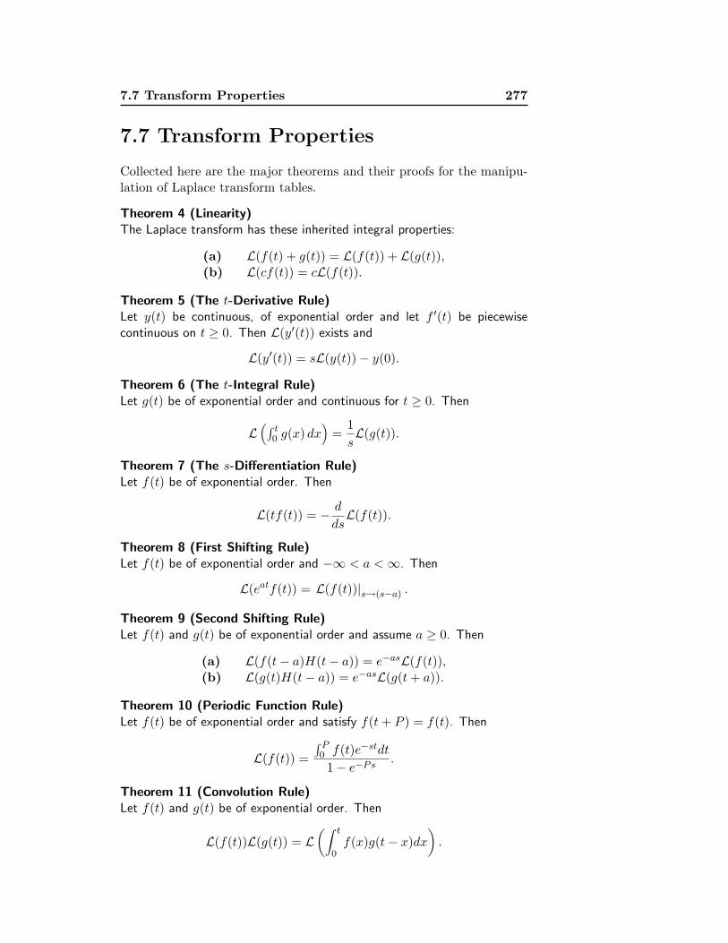
Collected here are the major theorems and their proofs for the manipu-lation of Laplace transform tables.

Theorem 4 (Linearity)The Laplace transform has these inherited integral properties:

(a) L(f(t) + g(t)) = L(f(t)) + L(g(t)),(b) L(cf(t)) = cL(f(t)).

Theorem 5 (The t-Derivative Rule)Let y(t) be continuous, of exponential order and let f ′(t) be piecewisecontinuous on t ≥ 0. Then L(y′(t)) exists and

L(y′(t)) = sL(y(t))− y(0).

Theorem 6 (The t-Integral Rule)Let g(t) be of exponential order and continuous for t ≥ 0. Then

L(∫ t

0 g(x) dx)

=1sL(g(t)).

Theorem 7 (The s-Differentiation Rule)Let f(t) be of exponential order. Then

L(tf(t)) = − d

dsL(f(t)).

Theorem 8 (First Shifting Rule)Let f(t) be of exponential order and −∞ < a < ∞. Then

L(eatf(t)) = L(f(t))|s→(s−a) .

Theorem 9 (Second Shifting Rule)Let f(t) and g(t) be of exponential order and assume a ≥ 0. Then

(a) L(f(t− a)H(t− a)) = e−asL(f(t)),(b) L(g(t)H(t− a)) = e−asL(g(t + a)).

Theorem 10 (Periodic Function Rule)Let f(t) be of exponential order and satisfy f(t + P ) = f(t). Then

L(f(t)) =∫ P0 f(t)e−stdt

1− e−Ps.

Theorem 11 (Convolution Rule)Let f(t) and g(t) be of exponential order. Then

L(f(t))L(g(t)) = L(∫ t

0f(x)g(t− x)dx

).


Proof of Theorem 4 (linearity):

LHS = L(f(t) + g(t)) Left side of the identity in (a).

=∫∞0

(f(t) + g(t))e−stdt Direct transform.

=∫∞0

f(t)e−stdt +∫∞0

g(t)e−stdt Calculus integral rule.

= L(f(t)) + L(g(t)) Equals RHS; identity (a) verified.

LHS = L(cf(t)) Left side of the identity in (b).

=∫∞0

cf(t)e−stdt Direct transform.

= c∫∞0

f(t)e−stdt Calculus integral rule.

= cL(f(t)) Equals RHS; identity (b) verified.

Proof of Theorem 5 (t-derivative rule): Already L(f(t)) exists, becausef is of exponential order and continuous. On an interval [a, b] where f ′ iscontinuous, integration by parts using u = e−st, dv = f ′(t)dt gives

∫ b

af ′(t)e−stdt = f(t)e−st|t=b

t=a −∫ b

af(t)(−s)e−stdt

= −f(a)e−sa + f(b)e−sb + s∫ b

af(t)e−stdt.

On any interval [0, N ], there are finitely many intervals [a, b] on each of whichf ′ is continuous. Add the above equality across these finitely many intervals[a, b]. The boundary values on adjacent intervals match and the integrals addto give

∫ N

0

f ′(t)e−stdt = −f(0)e0 + f(N)e−sN + s

∫ N

0

f(t)e−stdt.

Take the limit across this equality as N → ∞. Then the right side has limit−f(0) + sL(f(t)), because of the existence of L(f(t)) and limt→∞ f(t)e−st = 0for large s. Therefore, the left side has a limit, and by definition L(f ′(t)) existsand L(f ′(t)) = −f(0) + sL(f(t)).

Proof of Theorem 6 (t-Integral rule): Let f(t) =∫ t

0g(x)dx. Then f is of

exponential order and continuous. The details:

L(∫ t

0g(x)dx) = L(f(t)) By definition.

=1sL(f ′(t)) Because f(0) = 0 implies L(f ′(t)) = sL(f(t)).

=1sL(g(t)) Because f ′ = g by the Fundamental theorem of

calculus.

Proof of Theorem 7 (s-differentiation): We prove the equivalent relationL((−t)f(t)) = (d/ds)L(f(t)). If f is of exponential order, then so is (−t)f(t),therefore L((−t)f(t)) exists. It remains to show the s-derivative exists andsatisfies the given equality.

The proof below is based in part upon the calculus inequality∣∣e−x + x− 1

∣∣ ≤ x2, x ≥ 0.(1)


The inequality is obtained from two applications of the mean value theoremg(b)−g(a) = g′(x)(b−a), which gives e−x+x−1 = xxe−x1 with 0 ≤ x1 ≤ x ≤ x.

In addition, the existence of L(t2|f(t)|) is used to define s0 > 0 such thatL(t2|f(t)|) ≤ 1 for s > s0. This follows from the transform existence theoremfor functions of exponential order, where it is shown that the transform haslimit zero at s = ∞.

Consider h 6= 0 and the Newton quotient Q(s, h) = (F (s+h)−F (s))/h for thes-derivative of the Laplace integral. We have to show that

limh→0

|Q(s, h)− L((−t)f(t))| = 0.

This will be accomplished by proving for s > s0 and s + h > s0 the inequality

|Q(s, h)− L((−t)f(t))| ≤ |h|.

For h 6= 0,

Q(s, h)− L((−t)f(t)) =∫ ∞

0

f(t)e−st−ht − e−st + the−st

hdt.

Assume h > 0. Due to the exponential rule eA+B = eAeB , the quotient in theintegrand simplifies to give

Q(s, h)− L((−t)f(t)) =∫ ∞

0

f(t)e−st

(e−ht + th− 1

h

)dt.

Inequality (1) applies with x = ht ≥ 0, giving

|Q(s, h)− L((−t)f(t))| ≤ |h|∫ ∞

0

t2|f(t)|e−stdt.

The right side is |h|L(t2|f(t)|), which for s > s0 is bounded by |h|, completingthe proof for h > 0. If h < 0, then a similar calculation is made to obtain

|Q(s, h)− L((−t)f(t))| ≤ |h|∫ ∞

0

t2|f(t)e−st−htdt.

The right side is |h|L(t2|f(t)|) evaluated at s + h instead of s. If s + h > s0,then the right side is bounded by |h|, completing the proof for h < 0.

Proof of Theorem 8 (first shifting rule): The left side LHS of the equalitycan be written because of the exponential rule eAeB = eA+B as

LHS =∫ ∞

0

f(t)e−(s−a)tdt.

This integral is L(f(t)) with s replaced by s−a, which is precisely the meaningof the right side RHS of the equality. Therefore, LHS = RHS.

Proof of Theorem 9 (second shifting rule): The details for (a) are

LHS = L(H(t− a)f(t− a))

=∫∞0

H(t− a)f(t− a)e−stdt Direct transform.


=∫∞

aH(t− a)f(t− a)e−stdt Because a ≥ 0 and H(x) = 0 for x < 0.

=∫∞0

H(x)f(x)e−s(x+a)dx Change variables x = t− a, dx = dt.

= e−sa∫∞0

f(x)e−sxdx Use H(x) = 1 for x ≥ 0.

= e−saL(f(t)) Direct transform.

= RHS Identity (a) verified.

In the details for (b), let f(t) = g(t + a), then

LHS = L(H(t− a)g(t))

= L(H(t− a)f(t− a)) Use f(t− a) = g(t− a + a) = g(t).

= e−saL(f(t)) Apply (a).

= e−saL(g(t + a)) Because f(t) = g(t + a).

= RHS Identity (b) verified.

Proof of Theorem 10 (periodic function rule):

LHS = L(f(t))

=∫∞0

f(t)e−stdt Direct transform.

=∑∞

n=0

∫ nP+P

nPf(t)e−stdt Additivity of the integral.

=∑∞

n=0

∫ P

0f(x + nP )e−sx−nPsdx Change variables t = x + nP .

=∑∞

n=0 e−nPs∫ P

0f(x)e−sxdx Because f is P -periodic and

eAeB = eA+B .

=∫ P

0f(x)e−sxdx

∑∞n=0 rn Common factor in summation.

Define r = e−Ps.

=∫ P

0f(x)e−sxdx

11− r

Sum the geometric series.

=

∫ P

0f(x)e−sxdx

1− e−PsSubstitute r = e−Ps.

= RHS Periodic function identity verified.

Left unmentioned here is the convergence of the infinite series on line 3 of theproof, which follows from f of exponential order.

Proof of Theorem 11 (convolution rule): The details use Fubini’s in-tegration interchange theorem for a planar unbounded region, and thereforethis proof involves advanced calculus methods that may be outside the back-ground of the reader. Modern calculus texts contain a less general version ofFubini’s theorem for finite regions, usually referenced as iterated integrals. Theunbounded planar region is written in two ways:

D = {(r, t) : t ≤ r < ∞, 0 ≤ t < ∞},D = {(r, t) : 0 ≤ r < ∞, 0 ≤ r ≤ t}.

Readers should pause here and verify that D = D.


The change of variable r = x + t, dr = dx is applied for fixed t ≥ 0 to obtainthe identity

e−st∫∞0

g(x)e−sxdx =∫∞0

g(x)e−sx−stdx

=∫∞

tg(r − t)e−rsdr.

(2)

The left side of the convolution identity is expanded as follows:

LHS = L(f(t))L(g(t))

=∫∞0

f(t)e−stdt∫∞0

g(x)e−sxdx Direct transform.

=∫∞0

f(t)∫∞

tg(r − t)e−rsdrdt Apply identity (2).

=∫

Df(t)g(r − t)e−rsdrdt Fubini’s theorem applied.

=∫D f(t)g(r − t)e−rsdrdt Descriptions D and D are the same.

=∫∞0

∫ r

0f(t)g(r − t)dte−rsdr Fubini’s theorem applied.

Then

RHS = L(∫ t

0f(u)g(t− u)du

)

=∫∞0

∫ t

0f(u)g(t− u)due−stdt Direct transform.

=∫∞0

∫ r

0f(u)g(r − u)due−srdr Change variable names r ↔ t.

=∫∞0

∫ r

0f(t)g(r − t)dt e−srdr Change variable names u ↔ t.

= LHS Convolution identity verified.

Documents

Laplace Transform - University of Utahgustafso/2250LaplaceTheory.pdfChapter 7 Laplace Transform The Laplace transform can be used to solve diﬀerential equations. Be-sides being a