Embed Size (px)
Citation preview
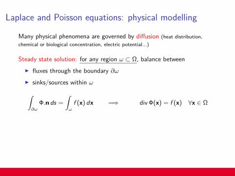
Laplace and Poisson equations: physical modelling
Many physical phenomena are governed by diffusion (heat distribution,chemical or biological concentration, electric potential...)
Steady state solution: for any region ω ⊂ Ω, balance betweenI fluxes through the boundary ∂ωI sinks/sources within ω∫∂ω
Φ.n ds =
∫ω
f (x) dx
=⇒ div Φ(x) = f (x) ∀x ∈ Ω
A common law: (Fourier’s law, Fick’s law) Φ = −k∇u where u is thedensity (temperature, concentration...) and k is the diffusivity coefficient
−div (k(x)∇u(x)) = f (x)
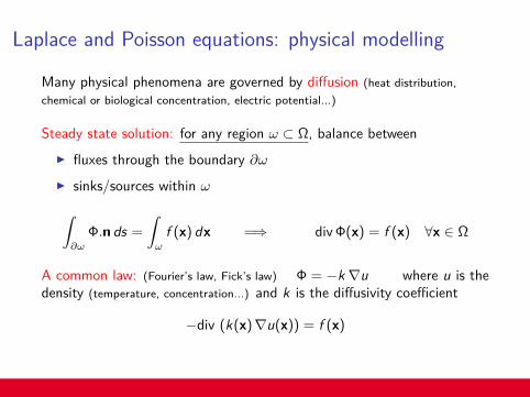
Laplace and Poisson equations: physical modelling
Many physical phenomena are governed by diffusion (heat distribution,chemical or biological concentration, electric potential...)
Steady state solution: for any region ω ⊂ Ω, balance betweenI fluxes through the boundary ∂ωI sinks/sources within ω∫∂ω
Φ.n ds =
∫ω
f (x) dx =⇒ div Φ(x) = f (x) ∀x ∈ Ω
A common law: (Fourier’s law, Fick’s law) Φ = −k∇u where u is thedensity (temperature, concentration...) and k is the diffusivity coefficient
−div (k(x)∇u(x)) = f (x)
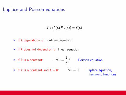
Laplace and Poisson equations
−div (k(x)∇u(x)) = f (x)
I If k depends on u: nonlinear equation
I If k does not depend on u: linear equation
I If k is a constant: −∆u =1k f Poisson equation
I If k is a constant and f = 0: ∆u = 0 Laplace equation,harmonic functions
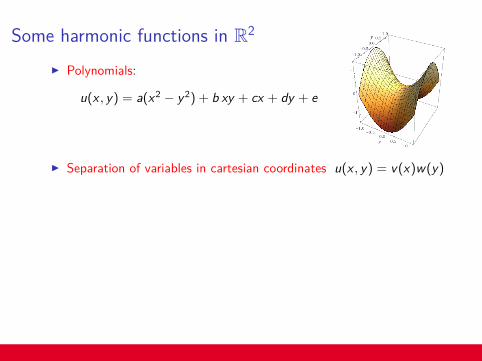
Some harmonic functions in R2
I Polynomials:
u(x , y) = a(x2 − y2) + b xy + cx + dy + e
I Separation of variables in cartesian coordinates u(x , y) = v(x)w(y)
elementary solutions:
u1λ(x , y) = (a cosλx + b sinλx)(ceλy + deλy )
u2λ(x , y) = (aeλx + beλx )(c cosλy + d sinλy)
∀λ 6= 0
hence any convergent sum of these functions
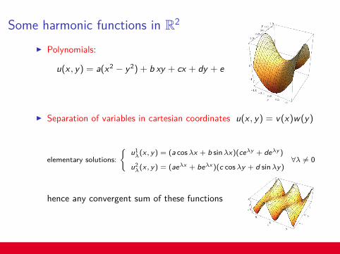
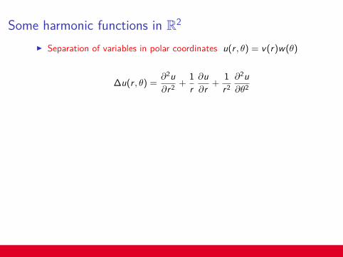
Some harmonic functions in R2
I Separation of variables in polar coordinates u(r , θ) = v(r)w(θ)
∆u(r , θ) =∂2u∂r2 +
1r∂u∂r +
1r2∂2u∂θ2
elementary solutionson R2 r (0, 0)
u0(r , θ) = c0 ln r + d0
un(r , θ) = (an cos nθ + bn sin nθ)
(cnrn +
dn
rn
)∀n ∈ N∗
hence any convergent sum of these functions
u0 u2 u4 u5
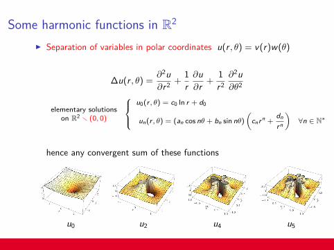
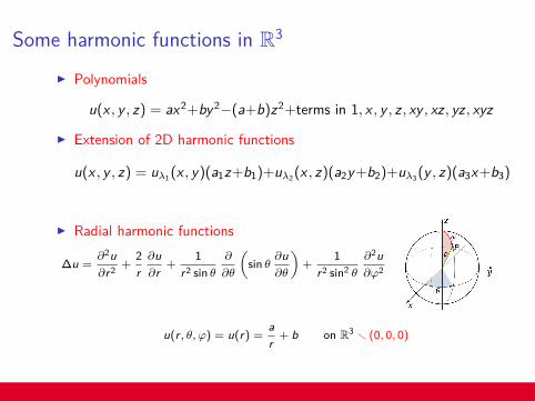
Some harmonic functions in R3
I Polynomials
u(x , y , z) = ax2+by2−(a+b)z2+terms in 1, x , y , z , xy , xz , yz , xyz
I Extension of 2D harmonic functions
u(x , y , z) = uλ1 (x , y)(a1z+b1)+uλ2 (x , z)(a2y+b2)+uλ3 (y , z)(a3x+b3)
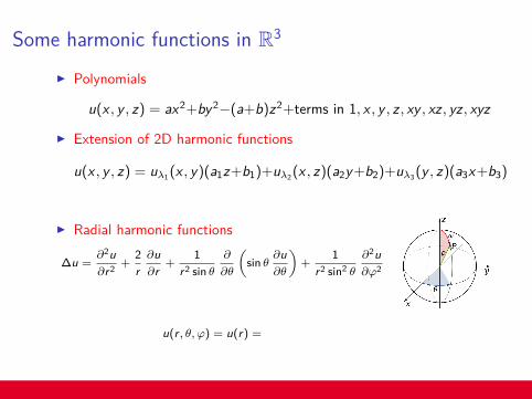
I Radial harmonic functions
∆u =∂2u∂r2 +
2r∂u∂r
+1
r2 sin θ∂
∂θ
(sin θ
∂u∂θ
)+
1r2 sin2 θ
∂2u∂ϕ2
u(r , θ, ϕ) = u(r) =ar
+ b on R3 r (0, 0, 0)
Some harmonic functions in R3
I Polynomials
u(x , y , z) = ax2+by2−(a+b)z2+terms in 1, x , y , z , xy , xz , yz , xyz
I Extension of 2D harmonic functions
u(x , y , z) = uλ1 (x , y)(a1z+b1)+uλ2 (x , z)(a2y+b2)+uλ3 (y , z)(a3x+b3)
I Radial harmonic functions
∆u =∂2u∂r2 +
2r∂u∂r
+1
r2 sin θ∂
∂θ
(sin θ
∂u∂θ
)+
1r2 sin2 θ
∂2u∂ϕ2
u(r , θ, ϕ) = u(r) =
ar
+ b on R3 r (0, 0, 0)
Some harmonic functions in R3
I Polynomials
u(x , y , z) = ax2+by2−(a+b)z2+terms in 1, x , y , z , xy , xz , yz , xyz
I Extension of 2D harmonic functions
u(x , y , z) = uλ1 (x , y)(a1z+b1)+uλ2 (x , z)(a2y+b2)+uλ3 (y , z)(a3x+b3)
I Radial harmonic functions
∆u =∂2u∂r2 +
2r∂u∂r
+1
r2 sin θ∂
∂θ
(sin θ
∂u∂θ
)+
1r2 sin2 θ
∂2u∂ϕ2
u(r , θ, ϕ) = u(r) =ar
+ b on R3 r (0, 0, 0)
Mean value property and maximum principle
I Mean value property:
u(x) =1
|B(x, r)|
∫B(x,r)
u(y) dy =1
|∂B(x, r)|
∫∂B(x,r)
u(σ) dσ ∀B(x, r) ⊂ Ω
An harmonic function is the average of its values over everysurrounding ball and sphere.
I Maximum principle: Let u an harmonic function. If u ∈ C2(Ω) andu ∈ C0(Ω), then u has no extreme values in Ω.
Harmonic functions in bounded domainsReminder: uniqueness of the solution of Laplace or Poisson problems inΩ ⊂ Rn: cf exercise session
div (k(x)∇u(x)) = f (x) in Ω
+ one of the following boundary conditions on ∂Ω
I Dirichlet: u = g on ∂Ω
I Neumann:∂u∂n
= h on ∂Ω
I Mixed: u = g on Γ0
∂u∂n
= h on Γ1where Γ0 ∪ Γ1 = ∂Ω and Γ0 ∩ Γ1 = ∅
−→ Uniqueness for Dirichlet and mixed BCs−→ No solution for Neumann BCs if
∫∂Ω
h(s)ds 6=∫
Ω
f (x)dx.No unique solution otherwise.
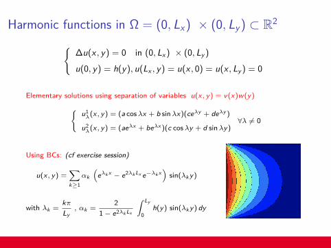
Harmonic functions in Ω = (0, Lx ) × (0, Ly ) ⊂ R2
∆u(x , y) = 0 in (0, Lx ) × (0, Ly )
u(0, y) = h(y), u(Lx , y) = u(x , 0) = u(x , Ly ) = 0
Elementary solutions using separation of variables u(x , y) = v(x)w(y)u1λ(x , y) = (a cosλx + b sinλx)(ceλy + deλy )
u2λ(x , y) = (aeλx + beλx )(c cosλy + d sinλy)
∀λ 6= 0
Using BCs: (cf exercise session)
u(x , y) =∑k≥1
αk(
eλk x − e2λk Lx e−λk x)
sin(λky)
with λk =kπLy
, αk =2
1− e2λk Lx
∫ Ly
0h(y) sin(λky) dy
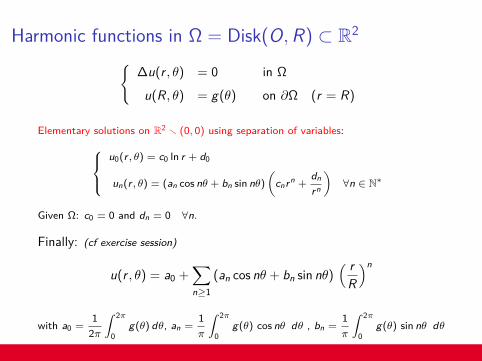
Harmonic functions in Ω = Disk(O,R) ⊂ R2
∆u(r , θ) = 0 in Ω
u(R, θ) = g(θ) on ∂Ω (r = R)
Elementary solutions on R2 r (0, 0) using separation of variables:u0(r , θ) = c0 ln r + d0
un(r , θ) = (an cos nθ + bn sin nθ)
(cnrn +
dn
rn
)∀n ∈ N∗
Given Ω: c0 = 0 and dn = 0 ∀n.
Finally: (cf exercise session)
u(r , θ) = a0 +∑n≥1
(an cos nθ + bn sin nθ)( r
R
)n
with a0 =1
2π
∫ 2π
0g(θ) dθ, an =
1π
∫ 2π
0g(θ) cos nθ dθ , bn =
1π
∫ 2π
0g(θ) sin nθ dθ
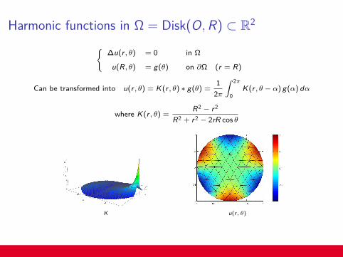
Harmonic functions in Ω = Disk(O,R) ⊂ R2
∆u(r , θ) = 0 in Ω
u(R, θ) = g(θ) on ∂Ω (r = R)
Can be transformed into u(r , θ) = K(r , θ) ∗ g(θ) =1
2π
∫ 2π
0K(r , θ − α) g(α) dα
where K(r , θ) =R2 − r2
R2 + r2 − 2rR cos θ
K u(r, θ)
−→ Illustration of the mean value property and of the maximum principle
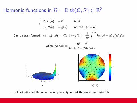
Harmonic functions in Ω = Disk(O,R) ⊂ R2
∆u(r , θ) = 0 in Ω
u(R, θ) = g(θ) on ∂Ω (r = R)
Can be transformed into u(r , θ) = K(r , θ) ∗ g(θ) =1
2π
∫ 2π
0K(r , θ − α) g(α) dα
where K(r , θ) =R2 − r2
R2 + r2 − 2rR cos θ
K u(r, θ)
−→ Illustration of the mean value property and of the maximum principle
Some properties of harmonic functions
I already seen: mean value property and maximum principle
I regularity In the 2-D case Ω = Disk(O,R):
u(r , θ) = K(r , θ) ∗ g(θ) with K(r , θ) =R2 − r2
R2 + r2 − 2rR cos θ
g ∈ C1(∂Ω) =⇒ u ∈ C∞(Ω)
(because (a ∗ b)′ = a ∗ b′ = a′ ∗ b for a, b ∈ C1 and K ∈ C∞)
I global influence of boundary values In the 2-D case Ω = Disk(O,R):
u(r , θ) = K(r , θ) ∗ g(θ) =1
2π
∫ 2π
0K(r , θ − α) g(α) dα
Any change, even very local, in the boundary data gwill modify the solution everywhere in Ω.
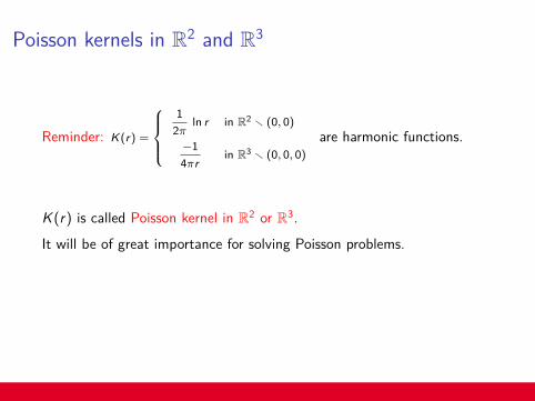
Poisson kernels in R2 and R3
Reminder: K(r) =
1
2πln r in R2 r (0, 0)
−14πr
in R3 r (0, 0, 0)
are harmonic functions.
K (r) is called Poisson kernel in R2 or R3.
It will be of great importance for solving Poisson problems.

Distributions for dummies
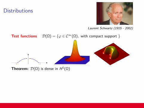
Distributions
Laurent Schwartz (1915 - 2002)
Test functions D(Ω) = ϕ ∈ C∞(Ω), with compact support
Theorem: D(Ω) is dense in H1(Ω)
Distributions Dual space D′(Ω), i.e. linear forms on D(Ω).T : D(Ω) −→ R
ϕ −→ T (ϕ), also denoted < T , ϕ >
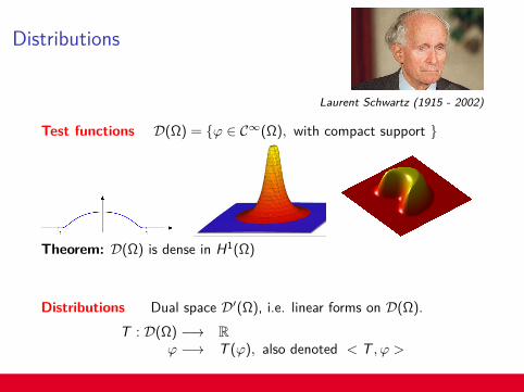
Distributions
Laurent Schwartz (1915 - 2002)
Test functions D(Ω) = ϕ ∈ C∞(Ω), with compact support
Theorem: D(Ω) is dense in H1(Ω)
Distributions Dual space D′(Ω), i.e. linear forms on D(Ω).T : D(Ω) −→ R
ϕ −→ T (ϕ), also denoted < T , ϕ >
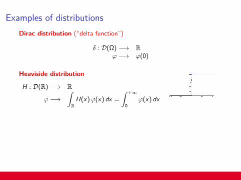
Examples of distributionsDirac distribution (“delta function”)
δ : D(Ω) −→ Rϕ −→ ϕ(0)
Heaviside distribution
H : D(R) −→ R
ϕ −→∫R
H(x)ϕ(x) dx =
∫ +∞
0ϕ(x) dx
Usual functions can be identified to distributions (f ⇐⇒ Tf )
∀f ∈ L1loc , < Tf , ϕ >=
∫Ω
f (x)ϕ(x) dx
−→ generalization of the notion of function.
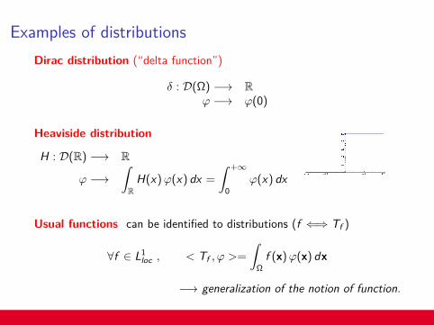
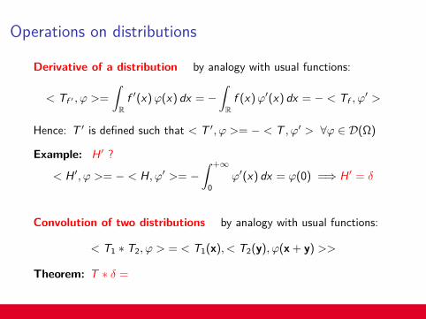
Operations on distributions
Derivative of a distribution by analogy with usual functions:
< Tf ′ , ϕ >=
∫R
f ′(x)ϕ(x) dx = −∫R
f (x)ϕ′(x) dx = − < Tf , ϕ′ >
Hence: T ′ is defined such that < T ′, ϕ >= − < T , ϕ′ > ∀ϕ ∈ D(Ω)
Example: H ′ ?
< H ′, ϕ >= − < H, ϕ′ >= −∫ +∞
0ϕ′(x) dx = ϕ(0) =⇒ H ′ = δ
Convolution of two distributions by analogy with usual functions:
< T1 ∗ T2, ϕ > = < T1(x), < T2(y), ϕ(x + y) >>
Theorem: T ∗ δ = T
Operations on distributions
Derivative of a distribution by analogy with usual functions:
< Tf ′ , ϕ >=
∫R
f ′(x)ϕ(x) dx = −∫R
f (x)ϕ′(x) dx = − < Tf , ϕ′ >
Hence: T ′ is defined such that < T ′, ϕ >= − < T , ϕ′ > ∀ϕ ∈ D(Ω)
Example: H ′ ?
< H ′, ϕ >= − < H, ϕ′ >= −∫ +∞
0ϕ′(x) dx = ϕ(0) =⇒ H ′ = δ
Convolution of two distributions by analogy with usual functions:
< T1 ∗ T2, ϕ > = < T1(x), < T2(y), ϕ(x + y) >>
Theorem: T ∗ δ =
T

Operations on distributions
Derivative of a distribution by analogy with usual functions:
< Tf ′ , ϕ >=
∫R
f ′(x)ϕ(x) dx = −∫R
f (x)ϕ′(x) dx = − < Tf , ϕ′ >
Hence: T ′ is defined such that < T ′, ϕ >= − < T , ϕ′ > ∀ϕ ∈ D(Ω)
Example: H ′ ?
< H ′, ϕ >= − < H, ϕ′ >= −∫ +∞
0ϕ′(x) dx = ϕ(0) =⇒ H ′ = δ
Convolution of two distributions by analogy with usual functions:
< T1 ∗ T2, ϕ > = < T1(x), < T2(y), ϕ(x + y) >>
Theorem: T ∗ δ = T
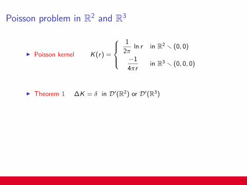
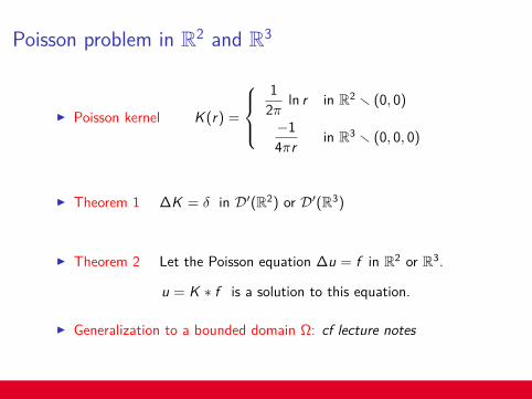
Poisson problem in R2 and R3
I Poisson kernel K (r) =
1
2π ln r in R2 r (0, 0)
−14πr in R3 r (0, 0, 0)
I Theorem 1 ∆K = δ in D′(R2) or D′(R3)
I Theorem 2 Let the Poisson equation ∆u = f in R2 or R3.
u = K ∗ f is a solution to this equation.
I Generalization to a bounded domain Ω: cf lecture notes
Poisson problem in R2 and R3
I Poisson kernel K (r) =
1
2π ln r in R2 r (0, 0)
−14πr in R3 r (0, 0, 0)
I Theorem 1 ∆K = δ in D′(R2) or D′(R3)
I Theorem 2 Let the Poisson equation ∆u = f in R2 or R3.
u = K ∗ f is a solution to this equation.
I Generalization to a bounded domain Ω: cf lecture notes


![of Laplace and Poisson equations [11]. In particular, we consider the case of four layer materials of different thermal conductivities. then useWe d finite difference](https://img.pdfslide.us/doc/110x75/5aebd7727f8b9a585f8e1bd2/of-laplace-and-poisson-equations-11-in-particular-we-consider-the-case-of-four.jpg)