This is a preprint of an article accepted for publication in Journal of the American Society for

Information Science and Technology copyright © 2010 (American Society for Information Science

and Technology)

Visualizing polysemy using LSA and the predication algorithm

Guillermo Jorge-Botana, José A. León, Ricardo Olmos

Universidad Autónoma de Madrid

Yusef Hassan-Montero

SCImago Research Group (CSIC)

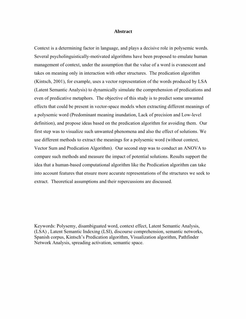
Abstract

Context is a determining factor in language, and plays a decisive role in polysemic words.

Several psycholinguistically-motivated algorithms have been proposed to emulate human

management of context, under the assumption that the value of a word is evanescent and

takes on meaning only in interaction with other structures. The predication algorithm

(Kintsch, 2001), for example, uses a vector representation of the words produced by LSA

(Latent Semantic Analysis) to dynamically simulate the comprehension of predications and

even of predicative metaphors. The objective of this study is to predict some unwanted

effects that could be present in vector-space models when extracting different meanings of

a polysemic word (Predominant meaning inundation, Lack of precision and Low-level

definition), and propose ideas based on the predication algorithm for avoiding them. Our

first step was to visualize such unwanted phenomena and also the effect of solutions. We

use different methods to extract the meanings for a polysemic word (without context,

Vector Sum and Predication Algorithm). Our second step was to conduct an ANOVA to

compare such methods and measure the impact of potential solutions. Results support the

idea that a human-based computational algorithm like the Predication algorithm can take

into account features that ensure more accurate representations of the structures we seek to

extract. Theoretical assumptions and their repercussions are discussed.

Keywords: Polysemy, disambiguated word, context effect, Latent Semantic Analysis, (LSA) , Latent Semantic Indexing (LSI), discourse comprehension, semantic networks, Spanish corpus, Kintsch’s Predication algorithm, Visualization algorithm, Pathfinder Network Analysis, spreading activation, semantic space.

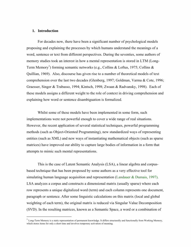
1. Introduction

For decades now, there have been a significant number of psychological models

proposing and explaining the processes by which humans understand the meanings of a

word, sentence or text from different perspectives. During the seventies, some authors of

memory studies took an interest in how a mental representation is stored in LTM (Long-

Term Memory1) forming semantic networks (e.g., Collins & Loftus, 1975; Collins &

Quillian, 1969). Also, discourse has given rise to a number of theoretical models of text

comprehension over the last two decades (Glenberg, 1997; Goldman, Varma & Cote, 1996;

Graesser, Singer & Trabasso, 1994; Kintsch, 1998; Zwaan & Radvansky, 1998). Each of

these models assigns a different weight to the role of context in driving comprehension and

explaining how word or sentence disambiguation is formalized.

Whilst some of these models have been implemented in some form, such

implementations were not powerful enough to cover a wide range of real situations.

However, the recent application of several statistical techniques, powerful programming

methods (such as Object-Oriented Programming), new standardized ways of representing

entities (such as XML) and new ways of instantiating mathematical objects (such as sparse

matrices) have improved our ability to capture large bodies of information in a form that

attempts to mimic such mental representations.

This is the case of Latent Semantic Analysis (LSA), a linear algebra and corpus-

based technique that has been proposed by some authors as a very effective tool for

simulating human language acquisition and representation (Landauer & Dumais, 1997).

LSA analyzes a corpus and constructs a dimensional matrix (usually sparse) where each

row represents a unique digitalized word (term) and each column represents one document,

paragraph or sentence. After some linguistic calculations on this matrix (local and global

weighting of each term), the original matrix is reduced via Singular Value Decomposition

(SVD). In the resulting matrices, known as a Semantic Space, a word or a combination of

1 Long-Term Memory is a static representation of permanent knowledge. It differs structurally and functionally from Working Memory, which stores items for only a short time and involves temporary activation of meaning.

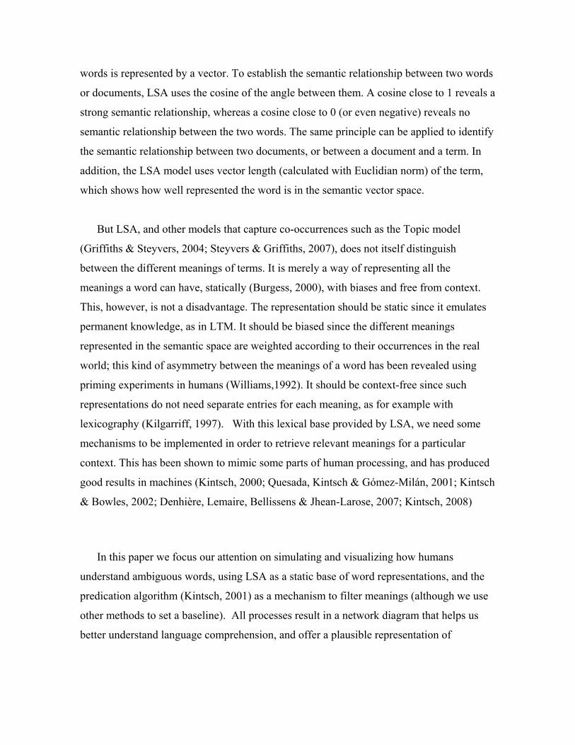
words is represented by a vector. To establish the semantic relationship between two words

or documents, LSA uses the cosine of the angle between them. A cosine close to 1 reveals a

strong semantic relationship, whereas a cosine close to 0 (or even negative) reveals no

semantic relationship between the two words. The same principle can be applied to identify

the semantic relationship between two documents, or between a document and a term. In

addition, the LSA model uses vector length (calculated with Euclidian norm) of the term,

which shows how well represented the word is in the semantic vector space.

But LSA, and other models that capture co-occurrences such as the Topic model

(Griffiths & Steyvers, 2004; Steyvers & Griffiths, 2007), does not itself distinguish

between the different meanings of terms. It is merely a way of representing all the

meanings a word can have, statically (Burgess, 2000), with biases and free from context.

This, however, is not a disadvantage. The representation should be static since it emulates

permanent knowledge, as in LTM. It should be biased since the different meanings

represented in the semantic space are weighted according to their occurrences in the real

world; this kind of asymmetry between the meanings of a word has been revealed using

priming experiments in humans (Williams,1992). It should be context-free since such

representations do not need separate entries for each meaning, as for example with

lexicography (Kilgarriff, 1997). With this lexical base provided by LSA, we need some

mechanisms to be implemented in order to retrieve relevant meanings for a particular

context. This has been shown to mimic some parts of human processing, and has produced

good results in machines (Kintsch, 2000; Quesada, Kintsch & Gómez-Milán, 2001; Kintsch

& Bowles, 2002; Denhière, Lemaire, Bellissens & Jhean-Larose, 2007; Kintsch, 2008)

In this paper we focus our attention on simulating and visualizing how humans

understand ambiguous words, using LSA as a static base of word representations, and the

predication algorithm (Kintsch, 2001) as a mechanism to filter meanings (although we use

other methods to set a baseline). All processes result in a network diagram that helps us

better understand language comprehension, and offer a plausible representation of

polysemy in the mind which is also helpful to NPL (Natural Language processing)

application designers.

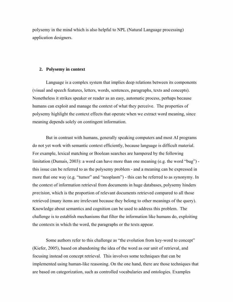
2. Polysemy in context

Language is a complex system that implies deep relations between its components

(visual and speech features, letters, words, sentences, paragraphs, texts and concepts).

Nonetheless it strikes speaker or reader as an easy, automatic process, perhaps because

humans can exploit and manage the context of what they perceive. The properties of

polysemy highlight the context effects that operate when we extract word meaning, since

meaning depends solely on contingent information.

But in contrast with humans, generally speaking computers and most AI programs

do not yet work with semantic context efficiently, because language is difficult material.

For example, lexical matching or Boolean searches are hampered by the following

limitation (Dumais, 2003): a word can have more than one meaning (e.g. the word “bug”) -

this issue can be referred to as the polysemy problem - and a meaning can be expressed in

more that one way (e.g. “tumor” and “neoplasm”) - this can be referred to as synonymy. In

the context of information retrieval from documents in huge databases, polysemy hinders

precision, which is the proportion of relevant documents retrieved compared to all those

retrieved (many items are irrelevant because they belong to other meanings of the query).

Knowledge about semantics and cognition can be used to address this problem. The

challenge is to establish mechanisms that filter the information like humans do, exploiting

the contexts in which the word, the paragraphs or the texts appear.

Some authors refer to this challenge as “the evolution from key-word to concept”

(Kiefer, 2005), based on abandoning the idea of the word as our unit of retrieval, and

focusing instead on concept retrieval. This involves some techniques that can be

implemented using human-like reasoning. On the one hand, there are those techniques that

are based on categorization, such as controlled vocabularies and ontologies. Examples

might be the word-net project, a human-based lexical database, or standards for

constructing domain-specific ontologies and knowledge-based applications with OWL or

XML-like editors such as PROTÉGÉ. And on the other hand there are statistical techniques

using patterns of word co-occurrence. Here we will focus our work on some techniques that

use statistical methods, such as LSA, and manage its representation in order to determine

which meaning of a word is intended using context. This is often referred as

disambiguation.

3. LSA as a basis for semantic processing.

LSA was first described as an information retrieval method (Deerwester et al.,

1990) but Landauer et al (1997) suggested that LSA could be a step towards resolving the

kind of human advantages that concern the capturing of deep relationships between words.

For instance, the problem called “poverty of the stimulus” or “Plato’s problem” asks how

people have more knowledge that they could reasonably extract from the information they

are exposed to. The solution is that a functional architecture such as LSA allows us to

make inductions from the environment – i.e. the reduced vectorial space representation of

LSA (explained in the introduction) allows us to infer that some words are connected with

one another even if they have not been found together in any sentence, paragraph,

conversation, etc. Furthermore, Landauer & Dumais use a simulation to show that for the

acquisition of knowledge about a word, the texts in which that word does not appear are

also important. In other words, we will acquire knowledge about lions by reading texts

about tigers and even about cars; the higher the frequency of a word, the more benefit

obtained from texts where it does not appear. These observations are in line with studies

that measures the capacity of nth order relations (second order and above) to induce

knowledge (Kontostathis & Pottenger, 2006; Lemaire & Denhière, 2006). 1st order relations

indicate a type of relationship where the two words occur in the same document of a

corpus. With 2nd order relations the two words do not occur together in a single document,

but both occur together with a common word. Higher relations indicate that words don’t

occur together or linked by a common term. The links lie at deeper levels. These studies

conclude that while first order relations can overestimate the eventual similarity between

terms, high-order co-occurrences - especially second order relations - play a significant

role.

Given such a “human-like” representation, it is not surprising perhaps that spaces

formed with LSA have proven adept at simulating human synonymy tasks - managing even

to capture the features of humans errors (Landauer & Dumais, 1997; Turney, 2001), and

also at simulating human graders’ assessments of a summary (Foltz, 1996; Landauer, 1998;

Landauer & Dumais, 1997, Landauer, Foltz & Laham, 1998; León, Olmos, Escudero,

Cañas & Salmerón, 2006).

The way in which LSA represents terms and texts is functionally quite similar to

others stochastic word representation methods. Each term is represented using a single

vector that contains all information pertaining to the contexts where it appears. Each vector

can be thought of as a box containing meanings. The most salient meaning is the most

frequent in the reference corpus (the corpus used to train LSA) followed by other less

frequent meanings. Supporting the idea that LSA vectors make massive use of context

information, some authors forced LSA to process material that had been tagged, marking

explicit differences in usage of the term in each context. The word “plane”, for example,

was given as many tags as meanings found (plane_noun, plane_verb). Such manipulation

results in worse performance (Serafín & DiEugenio, 2003; Wiemer-Hastings, 2000;

Wiemer-Hastings & Zipitria, 2001).

Nevertheless, Deerwester et al. (1990) draw attention to some limitations in

representing the phenomena of homonymy and polysemy. As explained above, a term is

represented in a single vector. This vector has certain coordinates. Since it has several

meanings, these are represented as an average of its meanings, weighted according to the

frequency of the contexts where it is found. If none of its actual meanings is close to that

mean, this could create a definition problem. This recalls the criticisms leveled at older

prototype-based models, which proposed the existence of a prototypical form - the sum of

the typical features of the members of that category. The criticism argues that if the

prototype is a cluster of features of a category, and bearing in mind the variability of the

typical elements, paradoxically the resulting prototype used to establish similarity is in fact

a very atypical member, perhaps even aberrant (Rosch & Mervis, 1975).

Theoretically the observations of Deerwester et al. (1990) are true, but less so if we

enhance LSA’s static representation by introducing some kind of mechanism that activates

meaning according to the active context at the moment of retrieval. As Burgess (2000)

claims in response to a criticism by Glenberg & Robertson (2000), LSA is not a process

theory, but rather a static representation of one kind of knowledge (the knowledge drawn

from the training corpus). To simulate the retrieval process we have to manage the net of

information supplied by LSA and exploit the representations of terms as well as those of

context. Using this mechanism, LSA has been attempted to simulate working memory

(Kintsch, 1998), paragraph reading (Denhière et al., 2007), processing whole sentences

(Kintsch, 2008) and even approaches to reasoning (Quesada et al., 2001) and understanding

predicative metaphors (Kintsch, 2000; Kintsch & Bowles, 2002).

All this simulations have to do with word disambiguation within a language

comprehension framework, with the assumption that the value of a word is evanescent and

takes on meaning only in interaction with other structures (Kintsch, 1998). There is no way

to disambiguate the word planta2 (plant) if we have no further data. Perhaps some general

meanings are automatically triggered in people’s minds, such as the plant kingdom, but we

can draw no definite conclusion in this respect. If someone asks us “¿Qué planta?” in an

elevator, an evanescent representation is generated which responds to a task demand, in a

context that had previously activated both linguistic and non-linguistic content. According

to Kintsch (2008), an ideal implementation of a mechanism that generates such an

evanescent representation requires only two components: flexible representation of words,

and a mechanism that can choose the correct form in a given context, taking into account 2 Planta in Spanish has several meanings in common with the word “plant” in English – for example it can be used to refer to the plant kingdom of living things, and to industrial or power installations. However, other senses are not shared: in Spanish planta also refers to the floors of an apartment block, for example.

representation biases. LSA can provide a good basis for representing words and texts in

terms of discrete values. It is a statistical data-driven technique offering flexible vector

representation, thus claiming some advantages over ontologies, for instance (Dumais,

2003). Its clear metric (operations with vectors) allows us to implement efficient algorithms

such as the predication algorithm (Kintsch, 2001).

In summary, storage and retrieval are not independent processes. The form in which

a term is stored, even if this seems very atypical or even aberrant, is not critical. What is

important is that, as in real life, linguistic structures take on the correct form, in line with

the context, at the time of retrieval. The goal is to manage the flexible representation well.

As Kintsch (1998) stated, knowledge is relatively permanent (the representation that

supplies LSA) but the meaning - the portion of the network that is activated - is flexible,

changeable and temporary.

4. The Predication Algorithm operating on LSA.

As we saw above, resolving polysemy involves retrieving the right meaning for a

word in its context, and ignoring irrelevant meaning. In order to do this, we need to

implement a mechanism that activates only that meaning of the word pertinent to the

retrieval context.

Suppose this structure (the word “planta” in the context of the word rosal):

“El rosal es una planta” (The rosebush is a plant)

One way to show the meaning of such a structure is by listing the semantic

neighbors closest to that structure (the vector that represents it). To extract these semantic

neighbors we need a procedure that calculates the cosine between this vector and all vector-

terms contained in the semantic space, and keeps a record of the n greatest values in a list -

the n most similar terms to the selected structure. Using this procedure we should obtain

neighbors related to the plant kingdom.

But the word “planta” has more meanings:

“La electricidad proviene de la planta” (The electricity comes from the plant)

“El ascensor viene de la planta 3” (The elevator came from the 3rd floor)

All these structures have the term “planta” as a common denominator, while this

same word takes on different meanings. We all know that in “El rosal es una planta” the

word “planta” does not have the same meaning as in “la electricidad proviene de la

planta”. The same term acquires one or other set of properties according to the contexts

that accompany it. In other words, the properties that give meaning to this term are

dependent on the context formed by the other words.

Let us take the proposition TERM [CONTEXT], assuming that the TERM takes on

some set of values depending on the CONTEXT. Both TERM and CONTEXT would be

represented by their own vectors in an LSA space.

To calculate the vector that represents the whole proposition, the common form of

LSA and other vector space techniques would simply calculate a new vector as the sum or

the “centroid” of the TERM vector and the CONTEXT vector.

Thus if the representation of the vectors according to their coordinates in the LSA space

were:

TERM vector= {t1,t2,t3,t4,t5,…,tn}

CONTEXT vector= {c1,c2,c3,c4,c5,…,cn}

Then the representation of the whole proposition would be:

PROPOSITION vector = {t1+c1, t2+c2, t3+c3, t4+c4, t5+c5,…, tn+cn}

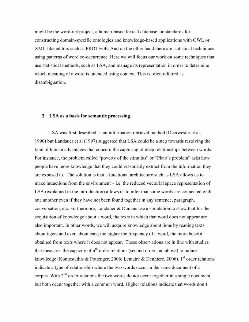
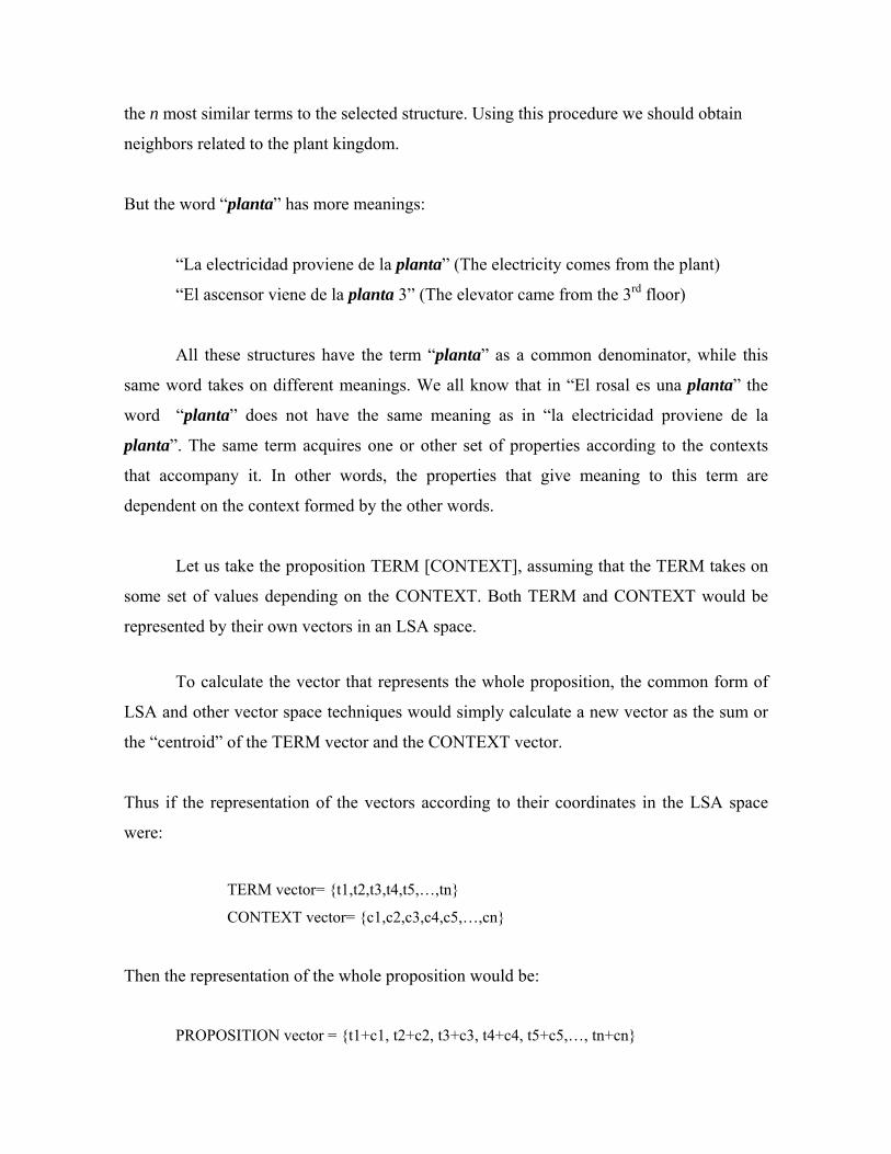
Due to the limitations of representation of meanings in LSA (Deerwester et al,

1990) explained earlier, this is not the best way to represent propositions, as it does not take

into account the term's dependence on the context. In other words, to compute the vector of

the entire proposition we do not need all the properties of the TERM (“planta”), only those

that relate to the meaning of the subject area (plant kingdom). What the centroid or Vector

sum does using the LSA method is to take all the properties - without discriminating

according to CONTEXT - and add them to those of the TERM.

Figure 1. Bias of the Centroid method between the words “Planta” and “Rosal”. Due to the vector length of the terms, the vector of Planta(Rosal) is close to the vector of Planta.

All the properties of the term “planta” are taken into account when calculating

the new vector. If, as in the above example (figure 1), the CONTEXT has a much lower

vector length than the TERM, and other meanings are better represented in the TERM,

the vector that represents the predication will not capture the actual intended meaning.

The meaning will be closer to the meaning of the context most represented in the LSA

space. With this simple vector sum method, the length of the term-vectors involved

dictates which semantic properties the vector representing the predication will take on.

We can therefore assume that the Vector Sum method fails to account for the true

meaning of certain structures, and tends to extract definitions of a given structure that

are subordinate to the predominant meaning.

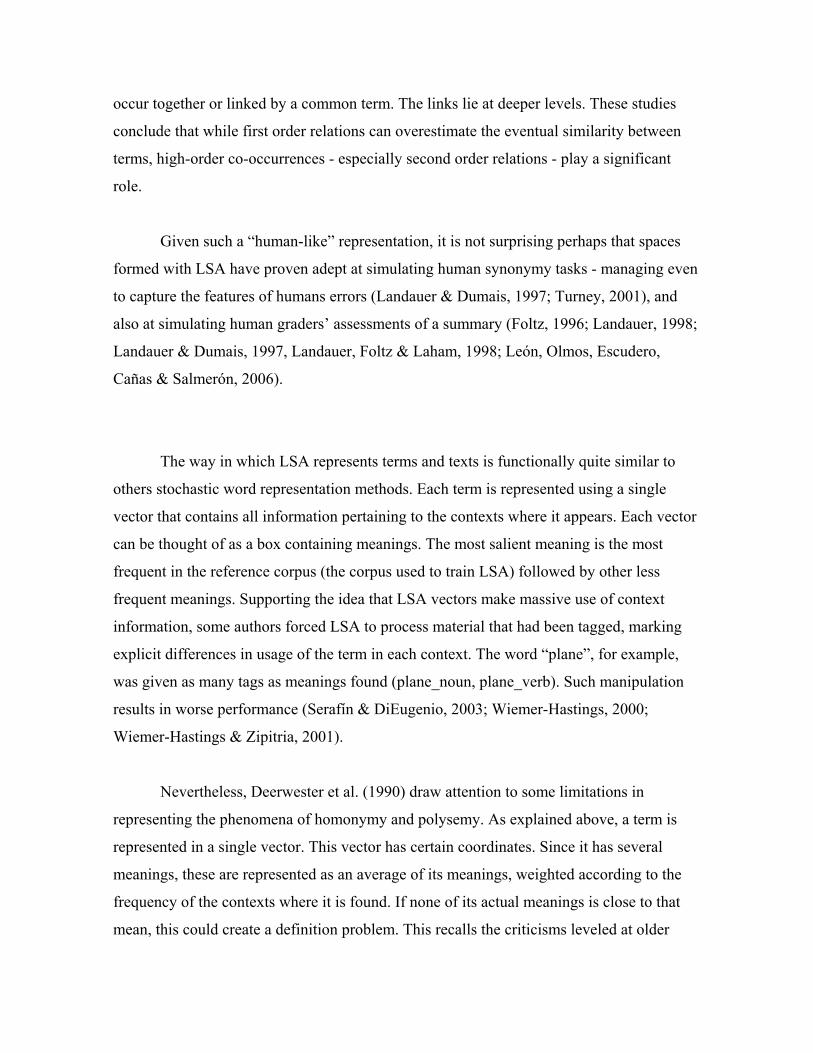
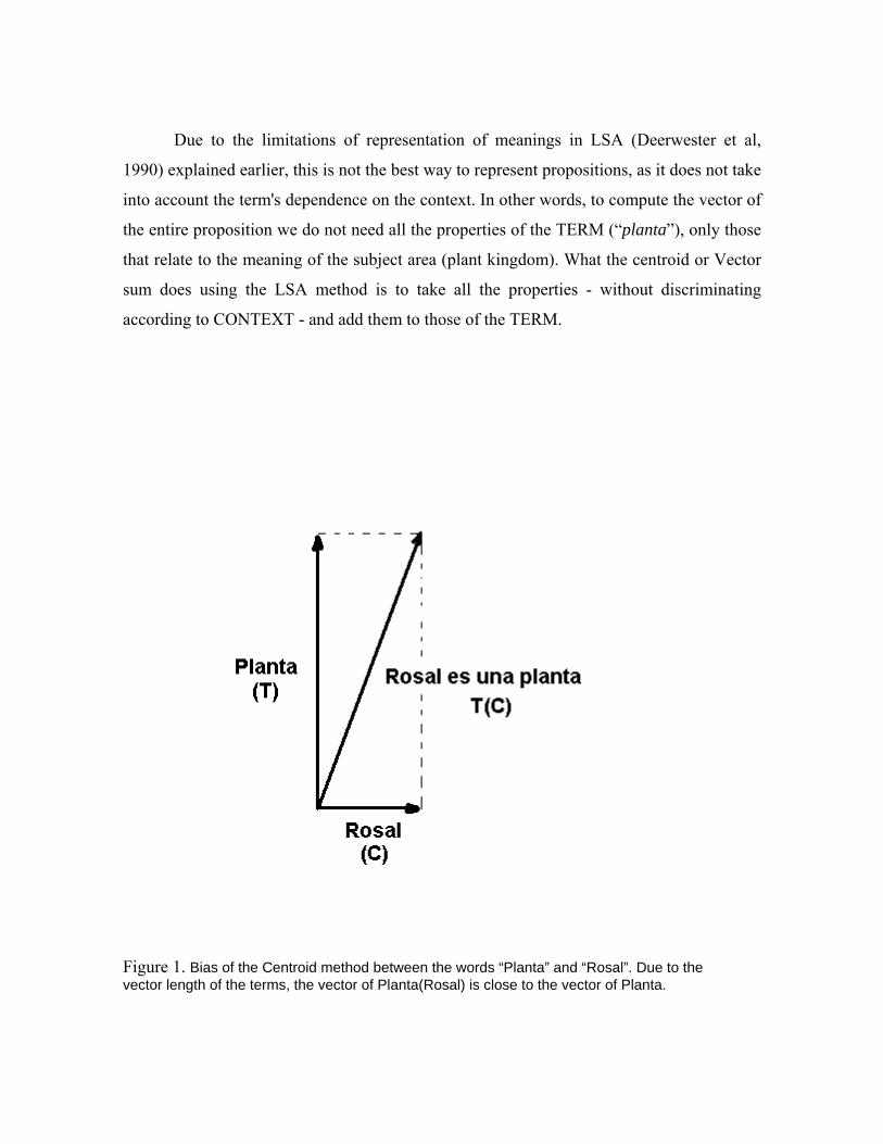
The Predication Algorithm (Kintsch, 2001), as its name suggests, was first used

on Predicate (Argument) propositions such as “The bridge collapsed”, “The plan

collapsed”, “The runner collapsed”. Nonetheless it may be used for general

Term(Context) structures. It aims to avoid this unwanted effect by following some

simple principles based on previous models of discourse comprehension such as

Construction-Integration nets (Kintsch, 1998). These principles are founded on node

activation rules that show how the final vector representing Term(Context) must be

formed with the vectors of the most highly activated words in the net. This activation

originates from the two terms (Term and Context-term), spreading to all words in the

semantic space (see figure 2). It is assumed that the more activated nodes, the more

words are pertinent to both Term (T) and Context (C) where T is constrained by C.

igure 2. Predication net between the words “Planta” (Plant) and “Rosal” (Rosebush).

To apply this algorithm it is necessary to have an LSA semantic space or some

FOnly neighbors of the Predicate relevant to the Argument will receive high activation: “vegetal” (vegetable) and “hoja” (leaf).

other vector space model as a starting point (see Kintsch, 2001 for an in-depth

presentation of the procedure). The steps are as follows: 1) find the n first terms with

greatest similarity to the Term (T), n being an empirical parameter. 2) Construct a net

with excitatory connections between each of those n terms and the Term (T), and

between each of those n terms and the Context (C). In each case the cosine is used as

the connection weighting value, i.e. a measure of similarity between the words. 3)

Some inhibitory connection between terms in the same layer can be implemented (terms

in the n first terms layer compete with one another for activation while they are

activated by Term (T) and Context (C) ) 4) Run the net until all nodes are recalculated

using a function that uses excitatory and inhibitory connections and promotes bilateral

excitation of each node (the net does not need a practice trial because the definitive

weights are those imposed by the LSA matrix). 5) The final vector for the predication is

calculated using the sum of the Term-vector (T), Context-Vector (C) and the p most

activated vector-nodes (again, p is an empirical value and p < n). The idea is that these

p terms are semantically related to both predicate and argument. The Context filters out

13

the n terms most closely related to the Term, and of these retain only the p terms most

pertinent to both predicate and argument.

Once the vector T(C) is established it can be compared with the terms in the

semantic space (using cosine or another similarity measure) to extract a list of semantic

neighbors - the meaning that is most closely related to the structure, and which would

contain a definition of it. This is the way that we use the predication algorithm to

resolve polysemy issues, where meaning is constrained by a particular context.

5. Objectives

The main aim of this article is to analyze the disambiguation of a polysemic

word in a retrieval context and reveal the biases that affect it.

Whilst several studies have used larger contextual units such as sentences or

paragraphs (Lemaire, Denhière, Bellisens & Jhean-Larose, 2006; Olmos, León, Jorge-

Botana & Escudero, 2009), we have used a single context word to modulate the

meaning of a polysemic word. Such a small window of context has been referred to in

other studies as a micro-context (Ide & Veronis, 1998). The word “plant” takes on one

meaning or another depending on the context word (“rosebush” or “energy”). Our

feeling is that combinations such as Word/Context-word3 are a more parsimonious way

to visualize the concepts, whilst preserving sensitivity to minor changes in context

word, and this is therefore the framework we use to investigate the behavior of vectorial

space models such as LSA.

We consider three problems concerning the system’s approach to processing

polysemic words (see Jorge-Botana, Olmos, León, 2009, for a previous study with a

specific domain corpus and different meanings of diagnostic terms). Problems emerge

during the extraction of a polysemic word’s meaning (as defined by its neighbors), both

with and without an explicit context.

3 Following the notation adopted in section 4, we refer to Word/Context-Word structures as [T(C)].

14

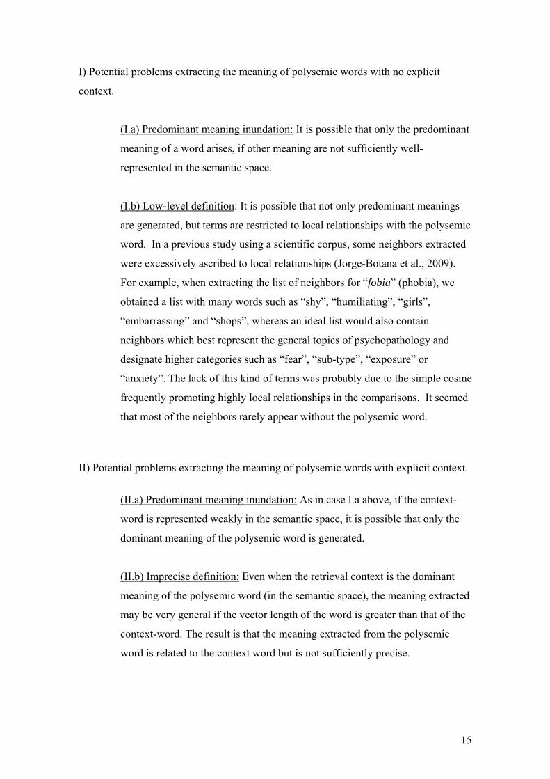
I) Potential problems extracting the meaning of polysemic words with no explicit

context.

(I.a) Predominant meaning inundation: It is possible that only the predominant

meaning of a word arises, if other meaning are not sufficiently well-

represented in the semantic space.

(I.b) Low-level definition: It is possible that not only predominant meanings

are generated, but terms are restricted to local relationships with the polysemic

word. In a previous study using a scientific corpus, some neighbors extracted

were excessively ascribed to local relationships (Jorge-Botana et al., 2009).

For example, when extracting the list of neighbors for “fobia” (phobia), we

obtained a list with many words such as “shy”, “humiliating”, “girls”,

“embarrassing” and “shops”, whereas an ideal list would also contain

neighbors which best represent the general topics of psychopathology and

designate higher categories such as “fear”, “sub-type”, “exposure” or

“anxiety”. The lack of this kind of terms was probably due to the simple cosine

frequently promoting highly local relationships in the comparisons. It seemed

that most of the neighbors rarely appear without the polysemic word.

II) Potential problems extracting the meaning of polysemic words with explicit context.

(II.a) Predominant meaning inundation: As in case I.a above, if the context-

word is represented weakly in the semantic space, it is possible that only the

dominant meaning of the polysemic word is generated.

(II.b) Imprecise definition: Even when the retrieval context is the dominant

meaning of the polysemic word (in the semantic space), the meaning extracted

may be very general if the vector length of the word is greater than that of the

context-word. The result is that the meaning extracted from the polysemic

word is related to the context word but is not sufficiently precise.

15

(II.c) Low-level definition: As in case I.b, the meaning facilitated by the

context-word may be generated, but the terms that represent this meaning are

related in a very local way with the polysemic word. These terms usually co-

occur in documents containing the polysemic word but never without it.

Problem I.a cannot be solved by computational systems (nor by humans), since

there is no explicit context to guide the correct meaning of a polysemic word. The

meaning extracted depends on the representation of each context in the semantic space.

When context is present, problems II.a and II.b, we propose, can be resolved by

applying Kintsch’s algorithm, as explained in section 4. In the case of problems I.b and

II.c, we propose to extract the neighbors that represent each meaning, adjusting the

simple cosine with the vector length of each term in the semantic space. This should

produce a more “high-level” neighbor list, with words from local relationships as well

as words that are less constrained by this kind of relationship. The function simply

weights the cosine measure according to the vector length of the terms (see section 7

below), thus ensuring a semantic network with some well-represented terms. This

method showed good results in a previous study using a domain-specific corpus (Jorge-

Botana et al., 2009), and our aim now is to apply it to a general domain corpus like

LEXESP.

We will use the following protocol:

In the first step, visualization, we visualize two meanings of two words in a

semantic network as an example. We will extract semantic neighbors using the two

methods outlined in section 4: Vector Sum and the Predication Algorithm. A base line

condition is also used extracting the neighbors for each word without context. This

procedure will allow us to visualize the probable main biases in the disambiguation of a

word using LSA or another vector-space method, (explained as problems II.a and II.b).

In the second step, to test the efficiency of the predication algorithm, we

examine a sample of polysemous items conjoined to their contexts. To compare its

efficiency, we conduct an ANOVA comparing the three conditions from the

visualization step, and numerically demonstrate the biases of these steps.

16

6. Visualizing the networks

6.1 Procedure

Following on from the work of authors who extracted and ordered all meanings of

some polysemic terms – for instance “apple” as a software company or a fruit

(Widdows & Dorow, 2002) – we represent polysemic meanings using a term-by-term

matrix (N×N) in which each cell represents the similarity of two terms from the list of

the n most similar terms (n first semantic neighbors) to the selected structure. For example, in

the case of “planta”, the term-by-term matrix would comprise the first n semantic

neighbors extracted. The resulting matrix was the input to Pathfinder4.

Our aim was to calculate the vector that represents the structure, its neighbors and

the similarity between them, using LSA as our static basis for word representation,

combined with some derived methods to solve the problems outlined in section 5.

The main procedure is as follows:

First, we drew the net of the polysemic word alone without any context word (e.g.

“plant”), in order to see the natural predominant meaning. This method involves

extracting a list of the term’s semantic neighbors5 and compiling a graph with them

(Pathfinder input). This diagram will highlight the problems that arise from (I.a

Predominant meaning inundation). The examples that we use are planta and partido6,

polysemic words without any context.

Second, we drew the net for the polysemic word T accompanied by two context

words (C1 and C2), (e.g. [plant (energy)] joined to [plant (rosebush)]). We calculate the

values of each structure, T(C1) and T(C2), with the simple vector sum of their

component vectors (Vplant + Venergy) and (Vplant + Vrosebush), and again extract the

semantically related neighbors for each structure. Finally, we compile a graph with all

4 We explain Pathfinder Network Analysis in section 7 (method) 5 Semantic neighbors of a term (or of a structure) are extracted comparing the vector of the term with each of the terms in the LSA semantic space. 6 Partido in Spanish has several meanings, the commonest being “political party” and “game/match” (only in the sense of playing competitively).

17

such neighbors. This will reveal problems II.a (Predominant meaning inundation) and

II.b (Imprecise definition). The actual examples we use are partido (fútbol,

nacionalista) [match/party (football, nationalist)] and planta (rosal, piso) [plant/floor

(rosebush, apartment)].

Third, we also drew the net for the polysemic word T accompanied by each of two

contexts C1 and C2, but this time calculating the values of the two structures, T(C1) and

T(C2), using Kintsch's predication algorithm (Kintsch, 2001). Again, we extract the

neighbors of each structure (both vectors calculated with Kintsch's predication

algorithm) and join them to make a graph. This will show the proposed solution to the

problems (II.a Predominant meaning inundation) and (II.b Imprecise). In other words,

we sought to verify whether Kintsch's predication algorithm is an effective method to

visualize the meanings of the two meanings together (compared to the first and second

conditions). The examples we use are again partido (fútbol, nacionalista) [match/party

(football, nationalist)] and planta (rosal, piso) [plant/floor (rosebush, apartment)].

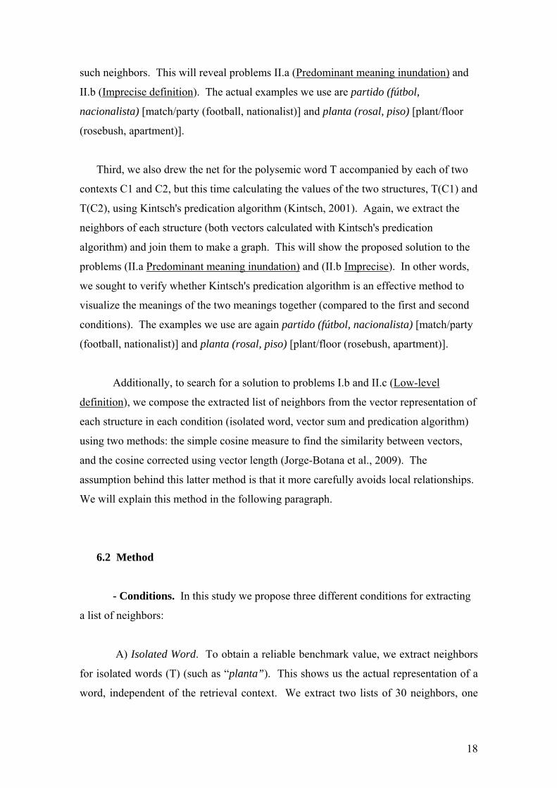
Additionally, to search for a solution to problems I.b and II.c (Low-level

definition), we compose the extracted list of neighbors from the vector representation of

each structure in each condition (isolated word, vector sum and predication algorithm)

using two methods: the simple cosine measure to find the similarity between vectors,

and the cosine corrected using vector length (Jorge-Botana et al., 2009). The

assumption behind this latter method is that it more carefully avoids local relationships.

We will explain this method in the following paragraph.

6.2 Method

- Conditions. In this study we propose three different conditions for extracting

a list of neighbors:

A) Isolated Word. To obtain a reliable benchmark value, we extract neighbors

for isolated words (T) (such as “planta”). This shows us the actual representation of a

word, independent of the retrieval context. We extract two lists of 30 neighbors, one

18

obtained using the simple cosine method, and the other with simple cosine adjusted for

vector length (explained below).

B) Word/Context-word vector sum. We need to contrast the predication

algorithm results with a baseline value, so we extracted neighbors of the vector of each

Word/Context-word, T(C1) and T(C2), using the classical method to represent complex

structures – the simple vector sum. We extracted 30 neighbors for each of the two

vectors and using each of the two methods (30 with simple cosine, 30 adjusting the

cosine according to vector length) and so obtained four lists with a total of 120 terms.

Repeated terms were deleted and reduced to a single representation, and the four lists

were then merged.

C) Word/Context-word with predication algorithm. In this condition we extract

semantic neighbors of each Word/Context-word, T(C1) and T(C2), using the predication

algorithm (Kintsch, 2001). We extract 30 neighbors of each of two predication vectors

with each of the two methods (30 with simple cosine, 30 adjusting the cosine according

to vector length), again obtaining four lists with a total of 120 terms. As before,

repeated terms were deleted and reduced to a single representation, and the four lists

were merged to produce the input to Pathfinder (the square matrix of terms).

- LSA, corpus and pre-processing. LSA was trained7 with the Spanish corpus

LEXESP8 (Sebastián, Cuetos, Carreiras & Martí, 2000) in a “by hand” lemmatized

version (plurals are transformed into their singular form and feminines are transformed

into their masculine form; all verbs are standardized into their infinitive form). The

LEXESP corpus contains texts of different styles and about different topics (newspaper

articles about politics, sports, narratives about specific topics, fragments from novels,

etc.). We chose sentences as units of processing: each sentence constituted a document

in the analysis. We deleted words that appear in less than seven documents to ensure

sufficiently reliable representations of the terms analyzed. The result was a term-

document matrix with 18,174 terms in 107,622 documents, to which we applied a 7 For calculations we used Gallito ®, an LSA tool implemented in our research group and developed in Microsoft® .Net (languages: VB.net and C#) integrated with Matlab ®. We also use this tool to implement the predication algorithm with net activation calculations (available at www.elsemantico.com). 8 In a study of Duñabeitia, J.A., Avilés, A., Afonso, O., Scheepers, C. & Carreiras, M.(2009), semantic pair similarities of the vector-words from this space have displayed good correlation with their analogous translations to English using spaces from an LSA model by http://lsa.colorado.edu/ and from HAL (Hyperespace Analogue to Lenguage) hosted at http://hal.ucr.edu/ , and also with judgment of Spanish natives speakers.

19

weighting function. This function attempts to estimate the importance of a term in

predicting the topic of documents in which it appears. The weighting functions

transform each raw frequency cell of the term-document matrix, using the product of a

local term weight and a global term weight. We applied the logarithm of raw frequency

as local weight and the formula of entropy as global term weight. We applied the SVD

algorithm to the final matrix, and reduced the three resulting matrices to 270

dimensions. The mean of the cosines between each term in the resultant semantic space

is 0.044, and the standard deviation is 0.07.

- Parameters for the predication algorithm. We have set n (n first terms with

greatest similarity to the Term T) at 5% of the total number of terms in our space, and k

(number of activated term nodes whose vector is taken to form the final representation

of the structure T(C)) equal to 5.

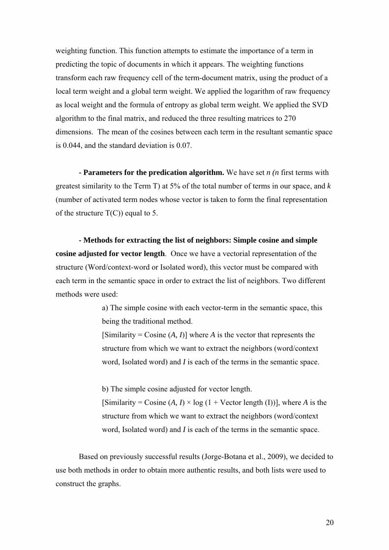
- Methods for extracting the list of neighbors: Simple cosine and simple

cosine adjusted for vector length. Once we have a vectorial representation of the

structure (Word/context-word or Isolated word), this vector must be compared with

each term in the semantic space in order to extract the list of neighbors. Two different

methods were used:

a) The simple cosine with each vector-term in the semantic space, this

being the traditional method.

[Similarity = Cosine (A, I)] where A is the vector that represents the

structure from which we want to extract the neighbors (word/context

word, Isolated word) and I is each of the terms in the semantic space.

b) The simple cosine adjusted for vector length.

[Similarity = Cosine (A, I) × log (1 + Vector length (I))], where A is the

structure from which we want to extract the neighbors (word/context

word, Isolated word) and I is each of the terms in the semantic space.

Based on previously successful results (Jorge-Botana et al., 2009), we decided to

use both methods in order to obtain more authentic results, and both lists were used to

construct the graphs.

20

Method for extracting neighbors

Structure and concrete examples used Cosine Cosine adjusted w/ vector length

Isolated word W Planta (Plant/Floor) 30 30 W(WC1) Planta (Rosal) [Plant/Floor (Rosebush)] 30 30 Word/Context word

Vector Sum W(WC2) Planta (Piso) [Plant/Floor (Apartment)] 30 30

W(WC1) Planta (Rosal) [Plant/Floor (Rosebush)] 30 30 Word/Context word with

predication algorithm W(WC2) Planta (Piso) [Plant/Floor (Apartment)] 30 30

Table 1. First, two lists of 30 neighbors were obtained for the isolated condition (W) - one with cosines and the other applying the correction to the cosine. Second, four lists are extracted from the Word/Context word structures formed with the Vector Sum condition - two for the first predication W (WC1) and two for the second predication W (WC2), one for each approach to extracting neighbors, cosines and corrected cosine. Thirdly, lists of the Word/Context word structures formed with the predication algorithm were extracted in the same way.

- Similarity Matrix. In order to understand and visually compare the semantic

structure of the networks, visualization techniques were applied. As input data, we used

a symmetrical N×N matrix that uses cosines to represent the semantic similarity of each

term with all others. These terms are all the words merged in the list of neighbors from

conditions in the previous steps (Isolated Word, Word/Context-word vector sum,

Word/Context-word with predication algorithm) . In other words, N is the total number

of terms in these three lists. For instance, in the case of Word/Context-word with

predication algorithm N counts the two lists for the first structure T(C1) plus the two

lists for the second structure T(C2) (Repeated terms of the merged list were deleted)

Following the methodology proposed by Börner, Chen and Boyack (2003), we

first need to reduce this n-dimensional space as an effective way to summarize the most

meaningful information represented in the network matrix. Analyzing scientific

literature on visualization reveals that the most useful dimensionality reduction

techniques are multidimensional scaling (MDS), Factor Analysis (FA), Self-Organizing

Maps (SOM), and Pathfinder Network Analysis (PFNets).

21

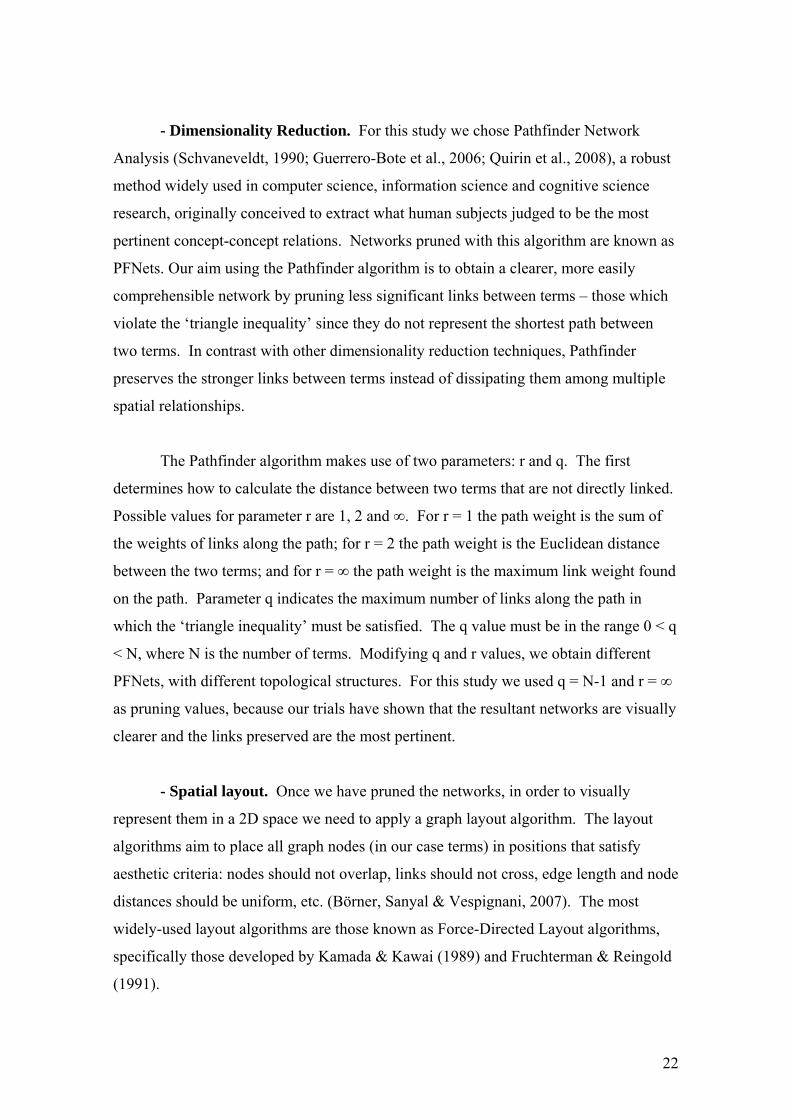
- Dimensionality Reduction. For this study we chose Pathfinder Network

Analysis (Schvaneveldt, 1990; Guerrero-Bote et al., 2006; Quirin et al., 2008), a robust

method widely used in computer science, information science and cognitive science

research, originally conceived to extract what human subjects judged to be the most

pertinent concept-concept relations. Networks pruned with this algorithm are known as

PFNets. Our aim using the Pathfinder algorithm is to obtain a clearer, more easily

comprehensible network by pruning less significant links between terms – those which

violate the ‘triangle inequality’ since they do not represent the shortest path between

two terms. In contrast with other dimensionality reduction techniques, Pathfinder

preserves the stronger links between terms instead of dissipating them among multiple

spatial relationships.

The Pathfinder algorithm makes use of two parameters: r and q. The first

determines how to calculate the distance between two terms that are not directly linked.

Possible values for parameter r are 1, 2 and ∞. For r = 1 the path weight is the sum of

the weights of links along the path; for r = 2 the path weight is the Euclidean distance

between the two terms; and for r = ∞ the path weight is the maximum link weight found

on the path. Parameter q indicates the maximum number of links along the path in

which the ‘triangle inequality’ must be satisfied. The q value must be in the range 0 < q

< N, where N is the number of terms. Modifying q and r values, we obtain different

PFNets, with different topological structures. For this study we used q = N-1 and r = ∞

as pruning values, because our trials have shown that the resultant networks are visually

clearer and the links preserved are the most pertinent.

- Spatial layout. Once we have pruned the networks, in order to visually

represent them in a 2D space we need to apply a graph layout algorithm. The layout

algorithms aim to place all graph nodes (in our case terms) in positions that satisfy

aesthetic criteria: nodes should not overlap, links should not cross, edge length and node

distances should be uniform, etc. (Börner, Sanyal & Vespignani, 2007). The most

widely-used layout algorithms are those known as Force-Directed Layout algorithms,

specifically those developed by Kamada & Kawai (1989) and Fruchterman & Reingold

(1991).

22

Whilst Fruchterman and Reingold’s algorithm is more suitable for representing

fragmented networks (i.e. a network comprising many components or sub graphs with

no connections between them), Kamada and Kawai’s algorithm has proved more

suitable for drawing non-fragmented PFNets (r=∞; q=N-1) (Moya-Anegón, Vargas,

Chinchilla, Corera, Gonzalez, Munoz et al., 2007). For our study Kamada and Kawai’s

algorithm might constitute a good option, but instead we chose a novel combination of

techniques to spatially distribute PFNets (r=∞; q=N-1) that demonstrate even better

results. We use Fruchterman and Reingold’s algorithm, but with a previous radial

layout. Radial layout is a well-known low-cost layout technique, where a focus node

was positioned in the centre of the visual space, and all other nodes were arranged in

concentric rings around it. Once radial layout is applied, then Fruchterman and

Reingold’s algorithm optimizes the spatial position of the nodes. These algorithms have

been implemented in a network viewer application, developed by the SCImago research

group, which is also being used for visual representation of scientific co-citation

networks (SCImago; 2007).

- Visual Attributes. In addition to the information represented by the term’s

spatial position and its connection with other terms, the graph contains other useful

information, encoded using two visual attributes: a) the node’s ellipse size indicates the

term’s vector length; b) the width of the link indicates the weight of the semantic

relationship.

- Related visualization studies for LSA with Pathfinder. It is difficult to

locate previous research that combined LSA with Pathfinder Network Analysis and

spatial layout algorithms. One pioneering example is a 1997 study by Chen (Chen &

Czerwinski, 1998), in which document-to-document semantic relationships (but not

term-to-term networks) are visually represented using PFNets and LSA. Kiekel, Cooke,

Foltz & Shope, (2001) applied PFNets and LSA to a log of verbal communication

among members of a work team – very different source data to the type used in this

study. Recently, Zhu and Chen (2007) have represented the terms of a collection of

documents using graphs, using LSA to represent the semantics of the corpus, but

without the Pathfinder pruning method.

6.3 Results and discussion

23

6.3.1 Results and discussion regarding PARTIDO (FÚTBOL,

NACIONALISTA) [match/party (football, nationalist)]

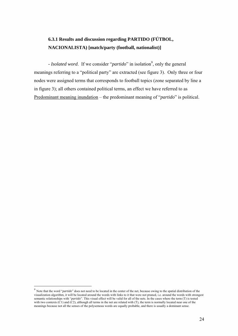
- Isolated word. If we consider “partido” in isolation9, only the general

meanings referring to a “political party” are extracted (see figure 3). Only three or four

nodes were assigned terms that corresponds to football topics (zone separated by line a

in figure 3); all others contained political terms, an effect we have referred to as

Predominant meaning inundation – the predominant meaning of “partido” is political.

9 Note that the word “partido” does not need to be located in the center of the net, because owing to the spatial distribution of the visualization algorithm, it will be located around the words with links to it that were not pruned, i.e. around the words with strongest semantic relationships with “partido”. This visual effect will be valid for all of the nets. In the cases where the term (T) is tested with two contexts (C1) and (C2), although all terms in the net are related with (T), the term is normally located near one of the meanings because not all the senses of the polysemous words are equally probable, and there is usually a dominant sense.

24

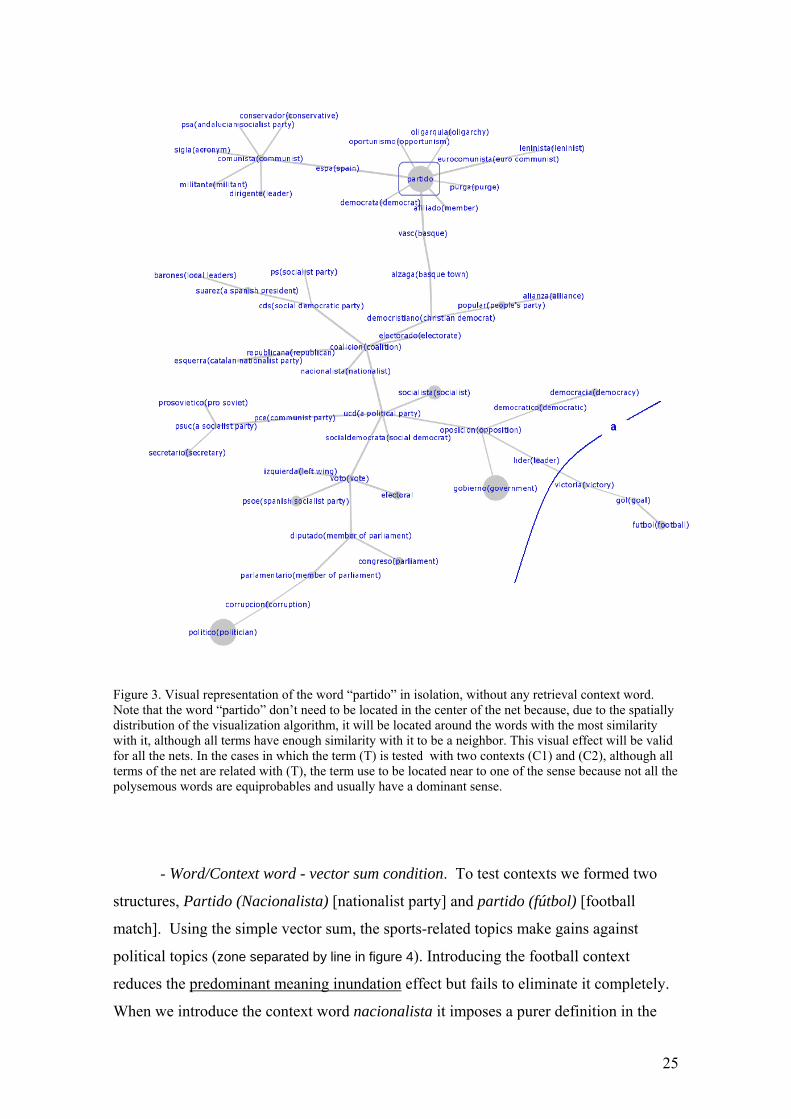
Figure 3. Visual representation of the word “partido” in isolation, without any retrieval context word. Note that the word “partido” don’t need to be located in the center of the net because, due to the spatially distribution of the visualization algorithm, it will be located around the words with the most similarity with it, although all terms have enough similarity with it to be a neighbor. This visual effect will be valid for all the nets. In the cases in which the term (T) is tested with two contexts (C1) and (C2), although all terms of the net are related with (T), the term use to be located near to one of the sense because not all the polysemous words are equiprobables and usually have a dominant sense.

- Word/Context word - vector sum condition. To test contexts we formed two

structures, Partido (Nacionalista) [nationalist party] and partido (fútbol) [football

match]. Using the simple vector sum, the sports-related topics make gains against

political topics (zone separated by line in figure 4). Introducing the football context

reduces the predominant meaning inundation effect but fails to eliminate it completely.

When we introduce the context word nacionalista it imposes a purer definition in the

25

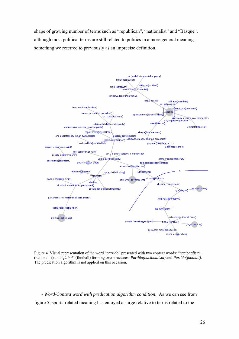
shape of growing number of terms such as “republican”, “nationalist” and “Basque”,

although most political terms are still related to politics in a more general meaning –

something we referred to previously as an imprecise definition.

Figure 4. Visual representation of the word “partido” presented with two context words: “nacionalista” (nationalist) and “fútbol” (football) forming two structures: Partido(nacionalista) and Partido(football). The predication algorithm is not applied on this occasion.

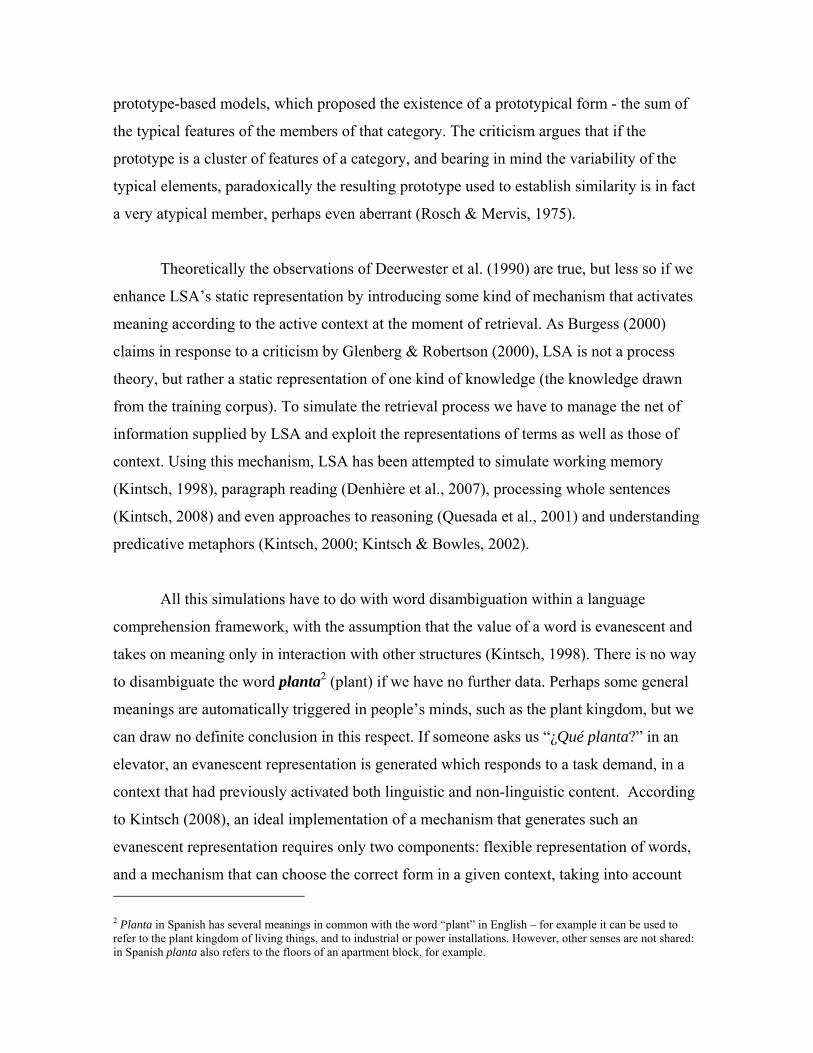
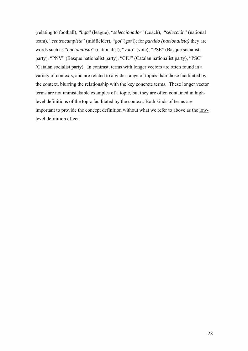
- Word/Context word with predication algorithm condition. As we can see from

figure 5, sports-related meaning has enjoyed a surge relative to terms related to the

26

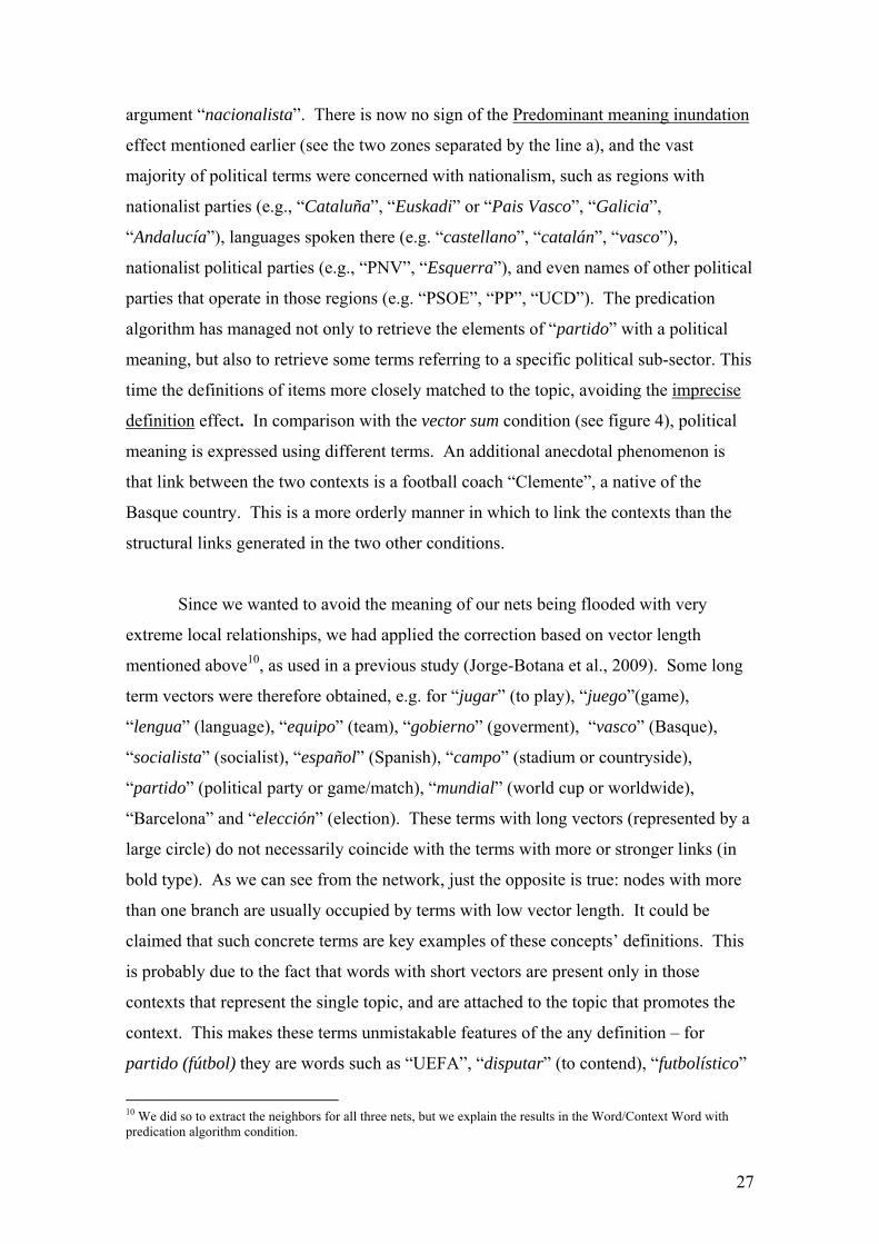
argument “nacionalista”. There is now no sign of the Predominant meaning inundation

effect mentioned earlier (see the two zones separated by the line a), and the vast

majority of political terms were concerned with nationalism, such as regions with

nationalist parties (e.g., “Cataluña”, “Euskadi” or “Pais Vasco”, “Galicia”,

“Andalucía”), languages spoken there (e.g. “castellano”, “catalán”, “vasco”),

nationalist political parties (e.g., “PNV”, “Esquerra”), and even names of other political

parties that operate in those regions (e.g. “PSOE”, “PP”, “UCD”). The predication

algorithm has managed not only to retrieve the elements of “partido” with a political

meaning, but also to retrieve some terms referring to a specific political sub-sector. This

time the definitions of items more closely matched to the topic, avoiding the imprecise

definition effect. In comparison with the vector sum condition (see figure 4), political

meaning is expressed using different terms. An additional anecdotal phenomenon is

that link between the two contexts is a football coach “Clemente”, a native of the

Basque country. This is a more orderly manner in which to link the contexts than the

structural links generated in the two other conditions.

Since we wanted to avoid the meaning of our nets being flooded with very

extreme local relationships, we had applied the correction based on vector length

mentioned above10, as used in a previous study (Jorge-Botana et al., 2009). Some long

term vectors were therefore obtained, e.g. for “jugar” (to play), “juego”(game),

“lengua” (language), “equipo” (team), “gobierno” (goverment), “vasco” (Basque),

“socialista” (socialist), “español” (Spanish), “campo” (stadium or countryside),

“partido” (political party or game/match), “mundial” (world cup or worldwide),

“Barcelona” and “elección” (election). These terms with long vectors (represented by a

large circle) do not necessarily coincide with the terms with more or stronger links (in

bold type). As we can see from the network, just the opposite is true: nodes with more

than one branch are usually occupied by terms with low vector length. It could be

claimed that such concrete terms are key examples of these concepts’ definitions. This

is probably due to the fact that words with short vectors are present only in those

contexts that represent the single topic, and are attached to the topic that promotes the

context. This makes these terms unmistakable features of the any definition – for

partido (fútbol) they are words such as “UEFA”, “disputar” (to contend), “futbolístico”

10 We did so to extract the neighbors for all three nets, but we explain the results in the Word/Context Word with predication algorithm condition.

27

(relating to football), “liga” (league), “seleccionador” (coach), “selección” (national

team), “centrocampista” (midfielder), “gol”(goal); for partido (nacionalista) they are

words such as “nacionalista” (nationalist), “voto” (vote), “PSE” (Basque socialist

party), “PNV” (Basque nationalist party), “CIU” (Catalan nationalist party), “PSC”

(Catalan socialist party). In contrast, terms with longer vectors are often found in a

variety of contexts, and are related to a wider range of topics than those facilitated by

the context, blurring the relationship with the key concrete terms. These longer vector

terms are not unmistakable examples of a topic, but they are often contained in high-

level definitions of the topic facilitated by the context. Both kinds of terms are

important to provide the concept definition without what we refer to above as the low-

level definition effect.

28

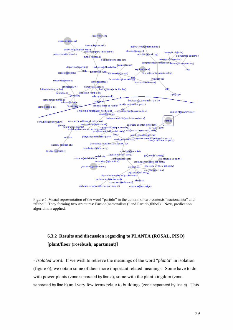
Figure 5. Visual representation of the word “partido” in the domain of two contexts “nacionalista” and “fútbol”. They forming two structures: Partido(nacionalista)” and Partido(fútbol)”. Now, predication algorithm is applied.

6.3.2 Results and discussion regarding to PLANTA (ROSAL, PISO)

[plant/floor (rosebush, apartment)]

- Isolated word. If we wish to retrieve the meanings of the word “planta” in isolation

(figure 6), we obtain some of their more important related meanings. Some have to do

with power plants (zone separated by line a), some with the plant kingdom (zone

separated by line b) and very few terms relate to buildings (zone separated by line c). This

29

time there is no single predominant meaning inundation effect as there is more balance

between meanings.

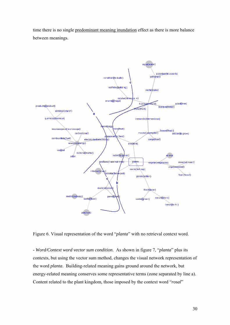
Figure 6. Visual representation of the word “planta” with no retrieval context word. - Word/Context word vector sum condition. As shown in figure 7, “planta” plus its

contexts, but using the vector sum method, changes the visual network representation of

the word planta. Building-related meaning gains ground around the network, but

energy-related meaning conserves some representative terms (zone separated by line a).

Content related to the plant kingdom, those imposed by the context word “rosal”

30

(rosebush) still occupy a strong position, albeit in a very general meaning – again we

see an imprecise definition effect.

Figure 7. Visual representation of the word “planta” for two contexts, “rosal” and “piso” forming two structures: Planta(rosal) and Planta(piso)”. The predication algorithm is not applied in this case.

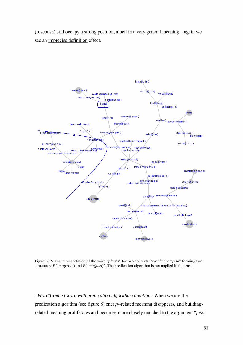
- Word/Context word with predication algorithm condition. When we use the

predication algorithm (see figure 8) energy-related meaning disappears, and building-

related meaning proliferates and becomes more closely matched to the argument “piso”

31

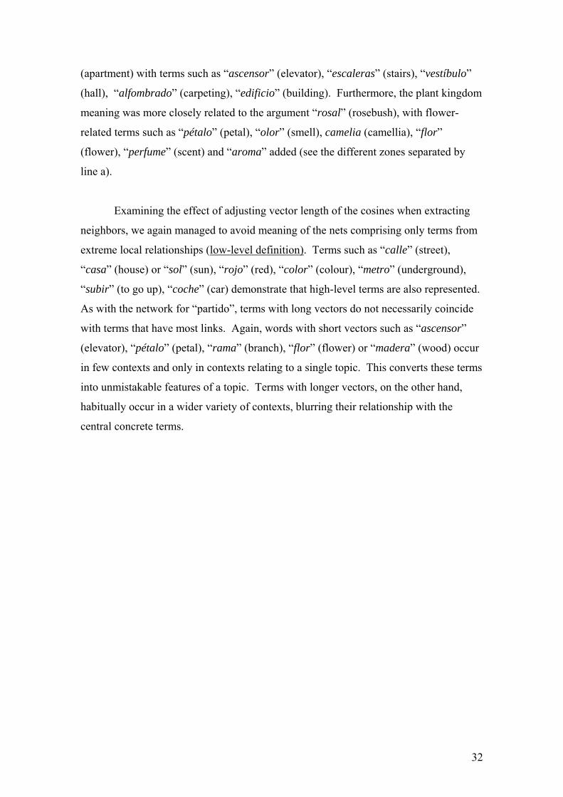
(apartment) with terms such as “ascensor” (elevator), “escaleras” (stairs), “vestíbulo”

(hall), “alfombrado” (carpeting), “edificio” (building). Furthermore, the plant kingdom

meaning was more closely related to the argument “rosal” (rosebush), with flower-

related terms such as “pétalo” (petal), “olor” (smell), camelia (camellia), “flor”

(flower), “perfume” (scent) and “aroma” added (see the different zones separated by

line a).

Examining the effect of adjusting vector length of the cosines when extracting

neighbors, we again managed to avoid meaning of the nets comprising only terms from

extreme local relationships (low-level definition). Terms such as “calle” (street),

“casa” (house) or “sol” (sun), “rojo” (red), “color” (colour), “metro” (underground),

“subir” (to go up), “coche” (car) demonstrate that high-level terms are also represented.

As with the network for “partido”, terms with long vectors do not necessarily coincide

with terms that have most links. Again, words with short vectors such as “ascensor”

(elevator), “pétalo” (petal), “rama” (branch), “flor” (flower) or “madera” (wood) occur

in few contexts and only in contexts relating to a single topic. This converts these terms

into unmistakable features of a topic. Terms with longer vectors, on the other hand,

habitually occur in a wider variety of contexts, blurring their relationship with the

central concrete terms.

32

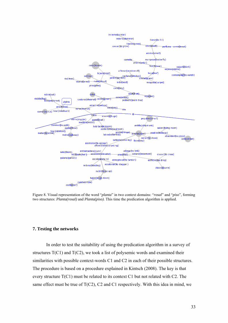
Figure 8. Visual representation of the word “planta” in two context domains: “rosal” and “piso”, forming two structures: Planta(rosal) and Planta(piso). This time the predication algorithm is applied.

7. Testing the networks

In order to test the suitability of using the predication algorithm in a survey of

structures T(C1) and T(C2), we took a list of polysemic words and examined their

similarities with possible context-words C1 and C2 in each of their possible structures.

The procedure is based on a procedure explained in Kintsch (2008). The key is that

every structure T(C1) must be related to its context C1 but not related with C2. The

same effect must be true of T(C2), C2 and C1 respectively. With this idea in mind, we

33

test the three conditions that correspond with the diagrams above, taking the isolated

condition as a base line.

7.1 Procedure

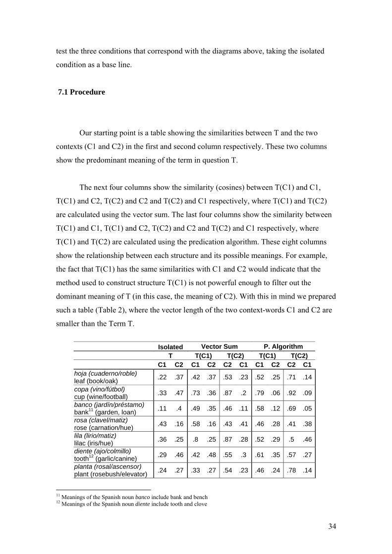
Our starting point is a table showing the similarities between T and the two

contexts (C1 and C2) in the first and second column respectively. These two columns

show the predominant meaning of the term in question T.

The next four columns show the similarity (cosines) between T(C1) and C1,

T(C1) and C2, T(C2) and C2 and T(C2) and C1 respectively, where T(C1) and T(C2)

are calculated using the vector sum. The last four columns show the similarity between

T(C1) and C1, T(C1) and C2, T(C2) and C2 and T(C2) and C1 respectively, where

T(C1) and T(C2) are calculated using the predication algorithm. These eight columns

show the relationship between each structure and its possible meanings. For example,

the fact that T(C1) has the same similarities with C1 and C2 would indicate that the

method used to construct structure T(C1) is not powerful enough to filter out the

dominant meaning of T (in this case, the meaning of C2). With this in mind we prepared

such a table (Table 2), where the vector length of the two context-words C1 and C2 are

smaller than the Term T.

Isolated Vector Sum P. Algorithm T T(C1) T(C2) T(C1) T(C2) C1 C2 C1 C2 C2 C1 C1 C2 C2 C1 hoja (cuaderno/roble) leaf (book/oak) .22 .37 .42 .37 .53 .23 .52 .25 .71 .14

copa (vino/fútbol) cup (wine/football) .33 .47 .73 .36 .87 .2 .79 .06 .92 .09

banco (jardín/préstamo) bank11 (garden, loan) .11 .4 .49 .35 .46 .11 .58 .12 .69 .05

rosa (clavel/matiz) rose (carnation/hue) .43 .16 .58 .16 .43 .41 .46 .28 .41 .38

lila (lirio/matiz) lilac (iris/hue) .36 .25 .8 .25 .87 .28 .52 .29 .5 .46

diente (ajo/colmillo) tooth12 (garlic/canine) .29 .46 .42 .48 .55 .3 .61 .35 .57 .27

planta (rosal/ascensor) plant (rosebush/elevator) .24 .27 .33 .27 .54 .23 .46 .24 .78 .14

11 Meanings of the Spanish noun banco include bank and bench 12 Meanings of the Spanish noun diente include tooth and clove

34

programa (software/tv) program (software/TV) .31 .36 .35 .36 .47 .31 .68 .3 .91 .1

caja (préstamo/envoltorio) box13 (loan, packaging) .15 .24 .28 .23 .33 .14 .63 .06 .63 .05

papel (actriz/cuaderno) paper14 (actress/notebook) .28 .26 .33 .26 .29 .28 .81 .05 .75 .22

cadena (tienda/tv) chain15 (shop/TV) .11 .81 .44 .75 .87 .11 .61 .18 .91 .08

partido (fútbol/nacionalista)party (football/Nationalist) .33 .43 .5 .39 .49 .32 .96 .06 .91 .07

bomba (misil/vapor) bomb16 (missile/steam) .37 .35 .82 .31 .74 .35 .85 .31 .77 .32

Table 2. Similarities between structures and each context

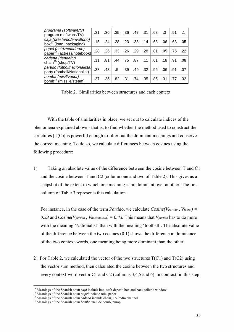
With the table of similarities in place, we set out to calculate indices of the

phenomena explained above - that is, to find whether the method used to construct the

structures [T(C)] is powerful enough to filter out the dominant meanings and conserve

the correct meaning. To do so, we calculate differences between cosines using the

following procedure:

1) Taking an absolute value of the difference between the cosine between T and C1

and the cosine between T and C2 (column one and two of Table 2). This gives us a

snapshot of the extent to which one meaning is predominant over another. The first

column of Table 3 represents this calculation.

For instance, in the case of the term Partido, we calculate Cosine(Vpartido , Vfútbol) =

0.33 and Cosine(Vpartido , Vnacionalista) = 0.43. This means that Vpartido has to do more

with the meaning ‘Nationalist’ than with the meaning ‘football’. The absolute value

of the difference between the two cosines (0.1) shows the difference in dominance

of the two context-words, one meaning being more dominant than the other.

2) For Table 2, we calculated the vector of the two structures T(C1) and T(C2) using

the vector sum method, then calculated the cosine between the two structures and

every context-word vector C1 and C2 (columns 3,4,5 and 6). In contrast, in this step

13 Meanings of the Spanish noun caja include box, safe-deposit box and bank teller’s window 14 Meanings of the Spanish noun papel include role, paper 15 Meanings of the Spanish noun cadena include chain, TV/radio channel 16 Meanings of the Spanish noun bomba include bomb, pump

35

we subtract the first cosine from the second in every structure to indicate the

strength of every structure’s correct meaning and filter out other meanings. In other

words, Cosine(T(C1), C1) minus Cosine(T(C1), C2) and Cosine(T(C2), C2) minus

Cosine(T(C2), C1). A negative value means that not only is the correct meaning not

represented strongly enough but also that other meanings are better represented. The

resulting values are in the second and third columns of Table 3.

For instance, the result of subtracting Cosine(Vpartido fútbol, Vfútbol) from Cosine(Vpartido

fútbol, Vnacionalista) is 0.11. This value will indicate the extent to which Vpartido fútbol has

the correct meaning and is not affected by the other meaning. On the other hand,

subtracting the first cosine (Vpartido nacionalista, Vnacionalista) from the second (Vpartido

nacionalista, Vfútbol) gives 0.17. This value will indicate the extent to which Vpartido

nacionalista has the correct meaning and is not affected by the other meaning.

3) The same procedure as 2) but this time with the columns where T(C1) and T(C2) has

been calculated the predication algorithm was used – that is, Cosine(T(C1), C1) minus

Cosine(T(C1), C2) and Cosine(T(C2), C2) minus Cosine(T(C2), C1) in columns 7,8,9

and 10 of Table 2. Again, a negative value means that not only is the correct meaning

not represented strongly enough but also that other meanings are better represented. The

resulting values are in the last two columns of Table 3.

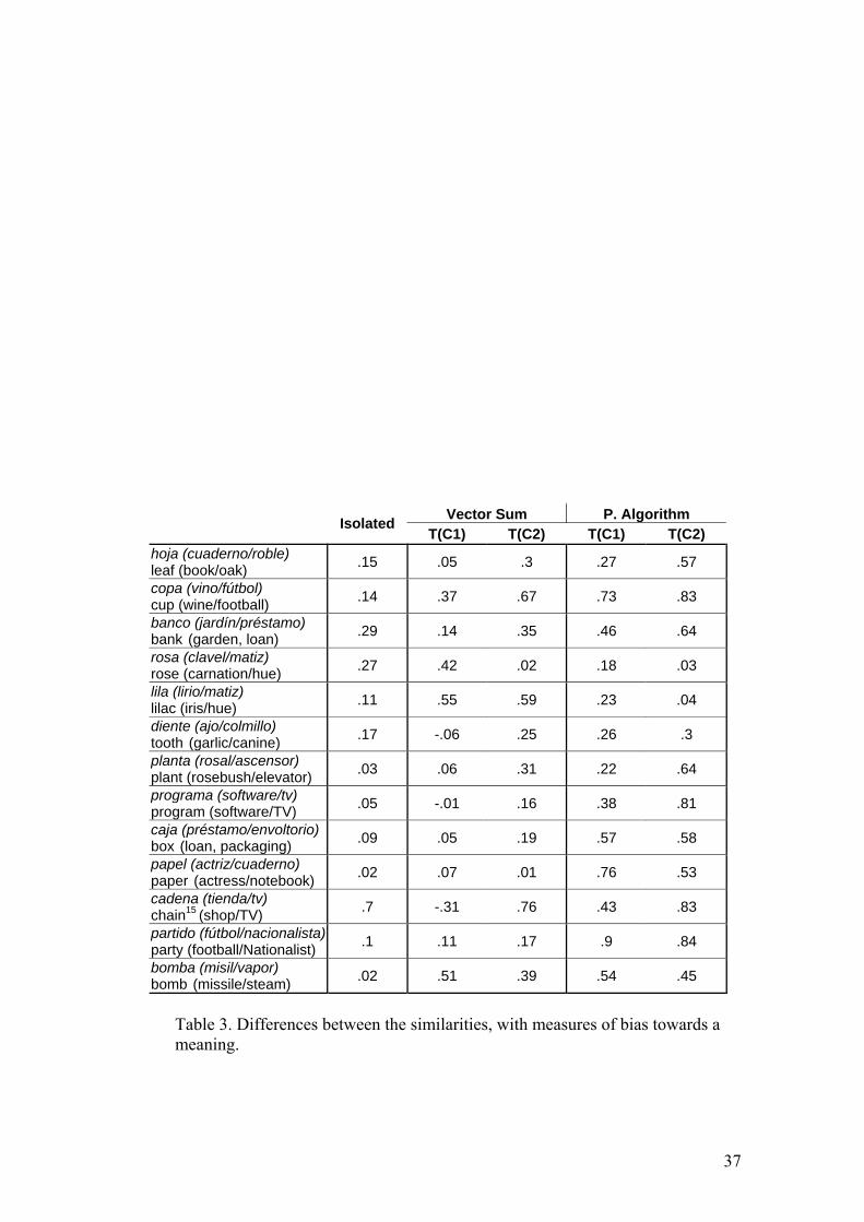
To summarise, the last four columns in Table 3 indicate the bias toward the

correct meaning represented by the vector of each structure. For example, .37 in the

T(C1) column indicates that the vector of T(C1) is biased toward the meaning of C1. On

the other hand, a value of .05 indicates that the vector of T(C1) is not biased toward the

meaning of C1 (because similarity with the other meaning is still strong). The Isolated

condition (the base line) is usually dramatically affected by the predominant meaning

effect, and for this reason the differences are irregular. If any of the other conditions

were affected by the predominant meaning effect, the differences will be also variable,

so the mean will be similar to the base line condition.

36

Vector Sum P. Algorithm

Isolated T(C1) T(C2) T(C1) T(C2)

hoja (cuaderno/roble) leaf (book/oak) .15 .05 .3 .27 .57

copa (vino/fútbol) cup (wine/football) .14 .37 .67 .73 .83

banco (jardín/préstamo) bank (garden, loan) .29 .14 .35 .46 .64

rosa (clavel/matiz) rose (carnation/hue) .27 .42 .02 .18 .03

lila (lirio/matiz) lilac (iris/hue) .11 .55 .59 .23 .04

diente (ajo/colmillo) tooth (garlic/canine) .17 -.06 .25 .26 .3

planta (rosal/ascensor) plant (rosebush/elevator) .03 .06 .31 .22 .64

programa (software/tv) program (software/TV) .05 -.01 .16 .38 .81

caja (préstamo/envoltorio) box (loan, packaging) .09 .05 .19 .57 .58

papel (actriz/cuaderno) paper (actress/notebook) .02 .07 .01 .76 .53

cadena (tienda/tv) chain15 (shop/TV) .7 -.31 .76 .43 .83

partido (fútbol/nacionalista) party (football/Nationalist) .1 .11 .17 .9 .84

bomba (misil/vapor) bomb (missile/steam) .02 .51 .39 .54 .45

Table 3. Differences between the similarities, with measures of bias towards a meaning.

37

With the table of the differences (Table 3), we conducted an ANOVA to see if

the two methods are significantly different in efficiency. Using the Isolated column as

our base line, the ANOVA had only one independent variable with three conditions:

Isolated, Vector Sum and Predication Algorithm. The dependent variable is the

difference represented in each cell of Table 3. We found homoscedasticity (FLevene(2,61)

= 2.45, p = .097), but we did not found normality in one of the conditions (Isolate). The

F-test is generally robust against violations of normality.

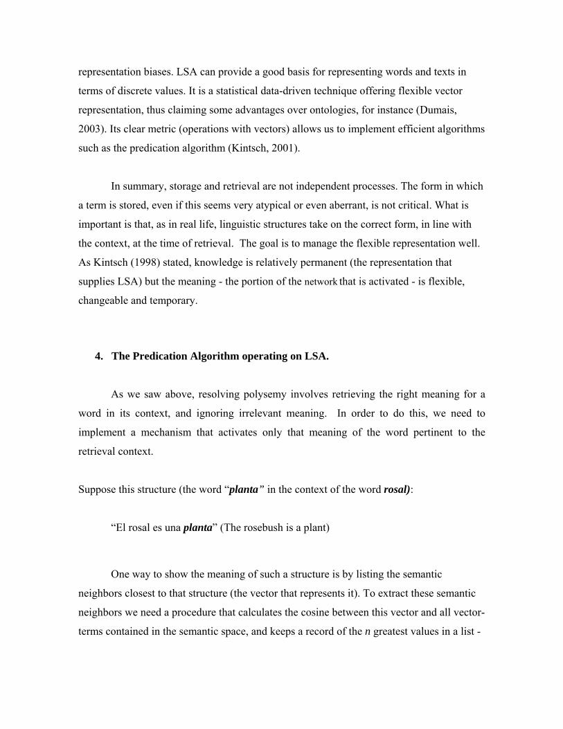
7.2 Results and discussion

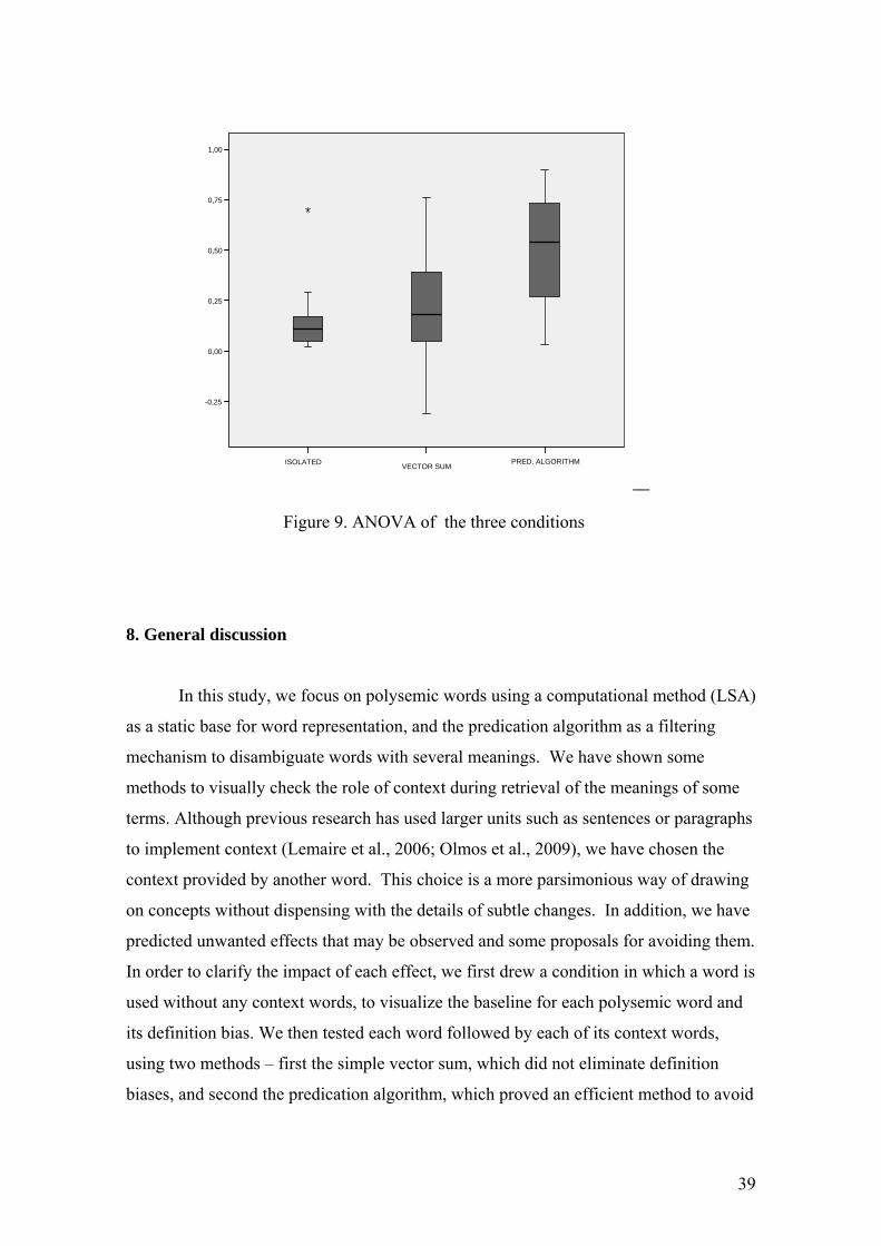
The ANOVA shows a main effect between the three conditions [F(2,61) =11.31,

MSE= .059, p < .05]. The means of Isolated, Vector Sum and Predication algorithm are

.16, .23 and .50 respectively. The Bonferroni correction shows that there are no

significant differences between Isolated and Vector Sum, while there is a significant

difference between Isolated and Predication Algorithm (P<.05) and between Vector

Sum and Predication Algorithm (P<.05). Although it displays more variability, the fact

that the Vector Sum condition shows no significant differences from the Isolated

condition indicates that the Vector Sum method is not usually powerful enough to cope

with the predominant meaning effect of T. In other words, when we calculate the

structures T(C1) and T(C2) with Vector Sum, it may be that one of them is still

dependent on the dominant meaning of T - the alternative meaning. The Predication

Algorithm appears to be less biased by the dominant meaning of the terms, and the

structures T(C1) and T(C2) are better represented.

38

__

PRED. ALGORITHM VECTOR SUMISOLATED

1,00

,2

0,75

0,50

0,25

0,00

-0 5

Figure 9. ANOVA of the three conditions

8. General discussion

In this study, we focus on polysemic words using a computational method (LSA)

as a static base for word representation, and the predication algorithm as a filtering

mechanism to disambiguate words with several meanings. We have shown some

methods to visually check the role of context during retrieval of the meanings of some

terms. Although previous research has used larger units such as sentences or paragraphs

to implement context (Lemaire et al., 2006; Olmos et al., 2009), we have chosen the

context provided by another word. This choice is a more parsimonious way of drawing

on concepts without dispensing with the details of subtle changes. In addition, we have

predicted unwanted effects that may be observed and some proposals for avoiding them.

In order to clarify the impact of each effect, we first drew a condition in which a word is

used without any context words, to visualize the baseline for each polysemic word and

its definition bias. We then tested each word followed by each of its context words,

using two methods – first the simple vector sum, which did not eliminate definition

biases, and second the predication algorithm, which proved an efficient method to avoid

39

some biases and to simulate comprehension of some predicative structures and term-

context structures (Kintsch, 2008).

Some interesting conclusions can be drawn from this study. One is related to the

representation of words independent of context (isolated condition) which may vary in

terms of how closely it matches reality. It is occasionally biased by how representative

the different meanings are within the semantic space. Sometimes, we find that only the

most representative meaning for this corpus are present (predominant meaning

inundation). Sometimes there are several meanings surrounding the word but lacking

detail (imprecise definition) – we see no more than general meanings of words, never

sub-domains. In other cases, the retrieved list of terms actually contains terms

unconnected with any of the meanings e.g. “mocito” (youngster) in figure 5, perhaps

due to the features of the vector in isolation from context. As explained in the

introduction, the dimensions of an LSA vector-term (especially the vectors of polysemic

words) are context-free and biased by the frequency with which a term occurs in the

document, resulting in a vector-prototype that is a cluster of features of all meanings.

This resulting vector-prototype used to establish similarity is in fact a very atypical

member and can sometimes promote spurious relations.

Another conclusion is related to the representation of words dependent of

context. In the case of Word/Context word, when we compound the vector with the

simple sum of the word and the context word, we find that sometimes the dominant

context has accounted for all the nodes (predominant meaning inundation). This was

probably caused by insufficient representation of one of the context words in the

semantic space. For instance, if the predominant meaning of a word is X and we add

another context Y which does not have sufficient vector length to compete with the

predominant meaning, then meaning Y will only result in a few terms and the

representation of X will be strengthened. This is why the meaning for the isolated word

condition and the meaning for a word followed by two context words might not vary –

as we observed for the word “partido”. If we use the simple sum of vectors, we can see

that the context “fútbol” (football) does not have sufficient vector length to retrieve

more than a few examples. In others cases (again with simple sum of vectors), the

visual representation of two predications conserves other meaning that does not

correspond to these contexts. For example when we extract the graph for Planta(rosal)

40

and Planta(piso), using simple sum of vectors the energy-related meaning of “planta” is

conserved in the shape of terms such as “químico” (chemical), “energía” (energy),

“central” (power plant) and “electricidad” (electricity). We can briefly summarize the

results of simple vector sum by saying that with this method we are exposed to the

influence of words’ vector lengths. We can sometimes obtain reasonable representations

but run the risk of obtaining only predominant or generic meanings. The fact that the

ANOVA detected no significant differences between the Isolated and Vector Sum

conditions in the second part of the article indicates that this affirmation may well be

true. It also confirms what we had seen visually: those structures calculated using the

Vector Sum method are still dependent on the dominant meaning of the terms.

When we draw the Word/Context word structures with the predication algorithm,

it seems we are able to correct these two problems. Content that does not match the

arguments was eliminated, and all pertinent meaning was well represented. This

advantageous method for drawing contexts relies on the way in which the algorithm

works. It primes terms extracted using the word which are more relevant to the context

words. This method aims to ensure that the final product contains vectors representing

the dimensions relevant to the word and to each retrieval context. This provides a very

detailed list of neighbors, representing ample examples of each argument which are well

distributed around the network. The fact that the ANOVA detected significant

differences between the Predication Algorithm and Vector Sum conditions in the second

part of the article indicates that the Predication Algorithm is less biased by the dominant

meanings, and operates more satisfactorily, as we had seen visually.

Concerning results of the vector length correction applied in previous studies

with a specific domain corpus (Jorge-Botana et al., 2009), we found that using a more

general corpus such as LEXESP, this technique also helps to ensure that some frequent

and important words are represented in the network. This is due to the actual correction

mechanism used to extract part of the list of neighbors. This mechanism gives the most

representative terms from the semantic space priority as neighbors (although this

priority is not mandatory). This means that representative nodes as well as local

relationships were represented visually, introducing some psychologically plausible

representation. Such frequent and important terms, however, do not necessarily form

more links. In fact the opposite is usually true: these frequent and important terms with

41

larger vectors do not usually occupy nodes with many links from other words. We have

concluded that this may be due to terms with larger vectors generally being more

general terms and occurring in a variety of contexts. For this reason they do not have

such a strong relationship with all the topic-related terms. On the other hand, terms

with shorter vectors often appear in a single context, making them unmistakable

features of that topic.

Conclusion

In general, what is remarkable about the LSA model is that the structural

similarity of the resulting vectors appears to parallel semantic similarities discerned by

human subjects between words in the corpus – sometimes with surprising accuracy.

Semantic spaces formed using LSA have offered pleasing results in synonym

recognition tasks (Landauer & Dumais, 1997; Turney, 2001), even simulating the

pattern of errors found in these tests (Landauer & Dumais, 1997). Using LSA it has

even been possible to study the rate of knowledge acquisition relating to a term, via

exposure to documents in which it does not appear (Landauer & Dumais, 1997). Such

correspondences would seem to suggest some non-arbitrary relationship between the

representations computed by LSA-type methods and our own cognitive representations

of word meaning. This ensures that LSA is a good basis for applying objective rules

from some models of cognitive processes and extracting reliable results

Since Kintsch (2001) proposed a psychologically plausible way to simulate

comprehension of predication – using LSA as a lexical base and applying objective

cognitive rules to it – we have a very intuitive means for formal understanding of what

the system does during comprehension of some linguistic structures, and the role of the

context of word retrieval. The predication algorithm applied to word pairs (Kintsch,

2001) and the predication algorithm applied to dependency relations within sentences

(Kintsch, 2008) are effective methods for differentially retrieving the meaning of words

according to the context imposed by arguments in propositions, and has proved better

than the traditional method of using simple sum of the vectors representing argument

and predicate.

42

In this study, we have presented a protocol for visualizing the contexts that a

word can take on, and have outlined the procedure to show the meanings of a word in

isolation, the meanings of a word with arguments but without using the predication

algorithm, and the meanings of a word with arguments using the predication algorithm.

A well-managed context ensures good representation of the meanings we wish to

retrieve, as shown intuitively by the visual nets, and rather more explicitly in the results

of the ANOVA.

This kind of human-based method could be used in retrieval applications or in

indexing or tagging machines, or even in the application of top-down processing rules –

for instance for improving confidence measures in speech recognition machines,

constraining the likelihood of a recognized term using the context. In addition, the nets

produced by these methods could be used as a visual information retrieval interface

(VIRI), allowing users to visually recognize the information that is needed, instead of

writing a query in the search boxes or providing an overview of a semantic domain, and

helping the user to know what information can be retrieved using the interface.

ACKNOWLEDGEMENTS

This work was supported by Grant SEJ2006-09916 from the Spanish Ministry of

Science and Technology and PSI 2009-31932 from the Spanish Ministry of Education

43

References

Börner, K., Chen, C., & Boyack, K. (2003). Visualizing knowledge domains. Annual Review of

Information Science & Technology, 37, 179–255.

Börner, K., Sanyal, S., & Vespignani, A. (2007). Network Science. Annual Review of

Information Science & Technology, 41, 537-607.

Burgess, C. (2000). Theory an operational definition in computational memory models: A

response to Glenberg and Robertson. Journal of Memory and Language, 43, 402-408.

Cederberg, S. & Widdows D. (2003). Using LSA and noun coordination information to improve

the precision and recall of automatic hyponymy extraction. Human Language Technology

Conference archive. In proceedings of the seventh conference on Natural language learning,

Edmonton, Canada, 111-118.

Chen, C. (1997). Tracking latent domain structures: An integration of Pathfinder and Latent

Semantic Analysis. Artificial Intelligence & Society, 11 (1-2), 48-62.

Chen, C. & Czerwinski, M. (1998). From latent semantics to spatial hypertext: An integrated

approach. In proceedings of the 9th ACM Conference on Hypertext and Hypermedia

(Hypertext '98), Pittsburgh, PA, 77-86.

Collins, A. & Loftus, J. (1975). A spreading activation theory of semantic memory.

Psychological Review, 82, 407-428.

Collins, A. & Quillian, M. R. (1969). Retrieval time from semantic memory. Journal of verbal

learning and verbal behavior 8 (2), 240-248.

Deerwester, S., Dumais, S. T., Furnas, G. W., Landauer, T. K., & Harshman, R. (1990).

Indexing By Latent Semantic Analysis. Journal of the American Society for Information

Science, 41, 391-407.

Denhière, G., Lemaire, B, Bellissens, C., & Jhean-Larose, S. (2007). A Semantic Space

Modeling Children’s Semantic Memory. In T. K. Landauer, D. McNamara, S. Dennis & W.

Kintsch (Eds.), The Handbook of Latent Semantic Analysis (pp. 143-167). Mahwah, NJ:

Erlbaum.

44

Duñabeitia, J.A., Avilés, A., Afonso, O., Scheepers, C. & Carreiras, M. (2009). Qualitative

differences in the representation of abstract versus concrete words: Evidence from the visual-

world paradigm. Cognition, 110, 284-292.

Dumais, S. T. (2003). Data-Driven approaches to information access. Cognitive Science, 2, 491-

524.

Fruchterman, T. M. & Reingold, E. M. (1991). Graph drawing by force-directed placement.

Software-Practice & Experience, 21, 1129–1164.

Foltz, P. W. (1996). Latent Semantic Analysis for text-based research. Behavior

Research Methods, Instruments and Computers, 28, 197-202.

Graesser, A., Singer, M. & Trabasso, T. (1994). Constructing inferences during narrative text

comprehension. Psychological Review, 101, 371-395.

Glenberg, A. M. (1997). What memory is for. Behavioral and Brain Sciences, 20, (1), 1-55.

Glenberg, A. M., & Robertson, D. A. (2000). Symbol grounding and meaning: A comparison of

high-dimensional and embodied theories of meaning. Journal of Memory and Language, 43,(3),

379–401.

Goldman, S., Varma, S., & Coté, N. (1996). Extending capacity-constrained construction

integration: Toward “smarter” and flexible models of text comprehension. In B. Britton & A.C.

Graesser (Eds.), Models of understanding text (pp. 73-113). Hillsdale, N.J.: Erlbaum.

Graesser, A., Singer, M., & Trabasso, T. (1994). Constructing inferences during narrative text

comprehension. Psychological Review, 101, 371-395.

Griffiths, T. L., & Steyvers, M. (2004). Finding scientific topics. Proceedings of the National Academy of Sciences, 101, 5228-5235.

Guerrero-Bote, V. et al. (2006). Binary Pathfinder: An improvement to the Pathfinder

algorithm. Information Processing & Management, 42 (6), December 2006, 1484-1490.

45

Ide, N., & Véronis, J. (1998). Word sense Disambiguation: The state of the Art. Computational

Linguistics, 24 (1), 1-41.

Jorge-Botana, G., Olmos, R., León J.A. (2009). Using LSA and the predication algorithm to

improve extraction of meanings from a diagnostic corpus. Spanish Journal of Psychology, 12,

(2), 414-440.

Kamada, T. & Kawai, S. (1989). An algorithm for drawing general undirected graphs.

Information Processing Letters, 31, 7–15.

Kiefer, B. (2005). Information Retrieval: Perspectives on Next Generation Search.

http://www.caseshare.com/articles-and-white-papers/72-catalyst-concept-search-perspectives-

on-next-generation-information-retrieval.html

Kiekel, P. A., Cooke, N. J., Foltz, P. W., & Shope, S. M. (2001). Automating measurement of

team cognition through analysis of communication data. In M. J. Smith, G. Salvendy, D. Harris,

and R. J. Koubek (Eds.), Usability Evaluation and Interface Design, pp. 1382-1386, Mahwah,

NJ: Lawrence Erlbaum Associates.

Kilgarriff, A. (1997). I don’t believe in word senses. Computers and the Humanities 31 (2), 91-113.

Kintsch, W. (1998). Comprehension: A paradigm for cognition. New York: Cambridge

University Press.

Kintsch, W. (2000). Metaphor comprehension: A computational theory. Psychonomic Bulletin

& Review, 7, 257-266.

Kintsch, W. (2001). Predication. Cognitive Science, 25, 173-202.

Kintsch, W. (2008). Symbol systems and perceptual representations. In M. de Vega, A. M. Glenberg, & A. C. Graesser (Eds.), Symbols and embodiment: Debates on meaning and cognition (pp. 145-164). Oxford: Oxford University Press.

Kintsch, W., & Bowles, A. (2002). Metaphor comprehension: What makes a metaphor difficult

to understand? Metaphor and Symbol, 17, 249-262.

46

Kontostathis, A., & Pottenger, W. M. (2006). A framework for understanding LSI performance.

Information Processing and Management, 42 (1), 56-73.

Landauer, T. K. (1998). Learning and representing verbal meaning: The Latent Semantic

Analysis Theory. Psychological Science, 7, 161-164.

Landauer, T. K., & Dumais, S. T. (1997). A solution to Plato's problem: the Latent Semantic

Analysis theory of the acquisition, induction, and representation of knowledge. Psychological

Review, 104, 211-240.

Landauer, T. K., Foltz, P. W., & Laham, D. (1998). An introduction to Latent

Semantic Analysis. Discourse Processes, 25, 259-284.

Lemaire, B., & Denhière, G. (2006). Effects of High-Order Co-occurrences on Word Semantic

Similarity. Current Psychology Letters, 18, 1.Web site: http://cpl.revues.org/document471.html.

Lemaire, B., Denhière, G., Bellissens, C., Jhean-Larose, S. (2006) A Computational Model for

Simulating Text Comprehension. Behavior Research Methods 38,(4), 628-637

León, J.A., Olmos, R., Escudero, I., Cañas, J.J. & Salmeron, L. (2006). Assessing short

summaries with human judgments procedure and latent semantic analysis in narrative and

expository texts. Behavior Research Methods, Instruments, and Computers, 38,(4), 616-627.

Moya-Anegón, F., Vargas, B., Chinchilla, Z., Corera, E., Gonzalez, A., Munoz, F., et al.

(2007). Visualizing the Marrow of Science. Journal of The American Society for Information

Science and Technology, 58, 2167-2179.

Olmos, R., León, J.A., Jorge-Botana, G. & Escudero, I. (2009). New algorithms assessing short

summaries in expository texts using Latent Semantic Analysis. Behavior Research Methods. 41,

(3), 944-950

Quesada, J., Kintsch, W., & Gómez-Milán, E. (2001). Theory of complex problem solving

using the vector space model. Latent Semantic Analysis applied to empirical results from

adaptation experiments. Cognitive Research with Microworlds, 147-158.

Quirin, A. et al. (2008). A new variant of the Pathfinder algorithm to generate large visual

science maps in cubic time. Information Processing and Management, 44, (4), 1611-1623.

47

Rosch, E., & Mervis, C., B. (1975). Family resemblances: Studies in the internal structures of

categories. Cognitive Psychology, 7, 573-605.

Salton, G. & McGill, M. J. (1983). Introduction to Modern Information Retrieval. McGraw-

Hill, New York, NY.

Sebastián-Gallés, N., Martí, M.A., Carreiras, M., & Cuetos, F. (2000). LEXESP: Una base de

datos informatizada del español. Barcelona. Universitat de Barcelona.

Serafin, R. & Di Eugenio. B. (2004). FLSA: Extending Latent Semantic Analysis with features

for dialogue act classification. Annual Meeting of the Association for Computational

Linguistics, Barcelona, Spain, July.

Schvaneveldt, R. W. (1990). Pathfinder associative networks: Studies in knowledge

organization. Norwood. NJ: Ablex.

SCImago. (2007). SJR — SCImago Journal & Country Rank. Retrieved September 10, 2008,

from http://www.scimagojr.com.

Steyvers, M., & Griffiths, T. (2007). Probabilistic topic models. In T. K. Landauer, D.

McNamara, S. Dennis & W. Kintsch (Eds.), Latent Semantic Analysis (pp. 427-448). Mahwah,

N.J.: Erlbaum.

Widdows, D., & Dorow, D. (2002). A Graph Model for Unsupervised Lexical Acquisition. In

Proceedings of the 19th International Conference on Computational Linguistics, Taipei, 1093-

1099.

Wiemer-Hastings, P. (2000). Adding syntactic information to LSA. In Proceedings of the 22nd

Annual Conference of the Cognitive Science Society, Erlbaum, Mahwah, NJ, 989–993.

Wiemer-Hastings, P., & Zipitria, I. (2001). Rules for syntax, vectors for semantics. In

Proceedings of the 23rd Cognitive Science Conference. Erlbaum, Mahwah, NJ.

Williams, J. N. (1992). Processing polysemous words in context: Evidence for interrelated meanings. Journal of Psycholinguistic Research, 21, 193–218.

48

Zhu, W., & Chen, C. (2007). Storylines: Visual exploration and analysis in latent semantic

spaces. Computers & Graphics, 31(3), 338-349.

Zwaan, R.A. & Radvansky G.A. (1998). Situation Models in Language Comprehension and

Memory. Psychological Bulletin, 123 (2), 162-185.

49