Embed Size (px)
Citation preview

Language as a Driver of Migration and
Trade using the Gravity Model:
A Comparative Analysis
Farhat Fasih
Master of Philosophy in Economics
Department of Economics
University of Oslo
May, 2018
(ii)
LANGUAGE AS A DRIVER OF MIGRATION AND TRADE USING THE GRAVITY MODEL:
A COMPARATIVE ANALYSIS
________________________________________________________________________________
FARHAT FASIH

(iii)
© Farhat Fasih, 2018
Language as a Driver of Migration and Trade using the Gravity Model:
A Comparative Analysis
Farhat Fasih
http://www.duo.uio.no/
Publisher: Reprosentralen, Universitetet i Oslo, Oslo – Norway

(iv)
Acknowledgments
This thesis marks the completion of my master’s degree and my tremendous journey at
the University of Oslo. Working on the thesis was both challenging and exciting for me.
Nevertheless, it has been a period of intense and progressive learning. I would not be
writing this preface today, had it not been for the support and encouragement of several
people who remained instrumental throughout the process. I would like to reflect on
the people who contributed to my writing, either directly or indirectly:
First and foremost, thank you to my advisor, Professor Andreas Moxnes, for
sharing his insightful knowledge, invaluable input, learning sessions, and
constant availability. I know you have been really patient and kind, thank you for
bearing with me!
I am indebted to this university for providing a platform of learning, for its
inspiring teachers, for all the facilities, and most importantly for the conducive
study environment.
I am particularly indebted to my parents for giving me a life full of opportunities,
and above all for their belief in me, as well as to my siblings for their never-ending
affection.
I am also thankful for my classmates and friends, for their study sessions, informal
discussions, and for simply being stress-busters. To Markus for his valuable
comments and Corina for her exhaustive proofreading.
Special thanks to my husband, for his zealous support, patience, and sharing my
responsibilities. Thanks, Fasih!
Finally, apart from all the gratitude and token of thanks, there is one beautiful
soul, my son Aiden, to whom I am really sorry. By this tender age of 18 months,
he has already learned my problems and taught me time management.
All the remaining mistakes and misprints are my sole responsibility.
Farhat Fasih
May 4, 2018

(v)
Abstract
Bilateral flows of both people (via migration) and goods (via trade) between countries
are imperative in the field of international economics and share many common
characteristics. This thesis attempts to examine the relative significance of language
proximity in terms of international migration and trade simultaneously, using the
standard gravity model. For this purpose, we use a dataset on migration and trade flows
from 223 host countries to 30 OECD destination countries in the period 1980-2006. We
find that language plays an important role in shaping migration patterns and boosting
trade volumes. In addition, the effect of gravity variables (i.e., GDP and geographical
distance) on migration and trade are in line with economic theory with small variations.
The estimation results successfully show that countries that are farther apart trade less
and have less migration between them, while economically larger countries are more
engaged in bilateral trade and attract more immigrants.

(vi)
TABLE OF CONTENTS
ACKNOWLEDGMENTS IV
ABSTRACT V LIST OF FIGURES AND TABLES VII
INTRODUCTION 1 1
THEORETICAL FRAMEWORK AND LITERATURE 2 4
ECONOMICS OF MIGRATION 2.1 4
MIGRATION AND CULTURAL PROXIMITY TO LANGUAGE 2.2 6
ECONOMICS OF INTERNATIONAL TRADE 2.3 8
INTERNATIONAL TRADE AND CULTURAL PROXIMITY TO LANGUAGE 2.4 10
GRAVITY MODELS OF INTERNATIONAL TRADE AND MIGRATION 2.5 11
EMPIRICAL MODEL 3 15
ESTIMATING EQUATIONS 3.1 15
ESTIMATION METHODOLOGY FOR GRAVITY EQUATIONS 3.2 20
DATA DESCRIPTION AND STRUCTURE 4 23
DATA SOURCES 4.1 23
DATA MERGING 4.2 28
DEPENDENT VARIABLE(S) 4.3 29
SUMMARY STATISTICS 4.4 29
EMPIRICAL RESULTS 5 32
MAIN RESULTS 5.1 32
ROBUSTNESS 5.2 40
ECONOMETRIC ISSUES 5.3 46
COMPARATIVE ANALYSIS 6 50
CONCLUSIONS 7 53
BIBLIOGRAPHY 56 APPENDIX 60

(vii)
LIST OF FIGURES AND TABLES
Figure 1 Multi-stage Economic Model of Migration ........................................................... 5
Figure 2 Multi-dimensional Explanation to Migration-Decision ........................................... 5
Figure 3 Determinants of Bilateral Trade Flows ................................................................ 9
Figure 4 Migration Flows to selected OECD Countries from all world, 1980-2006 .............. 24
Figure 5 Trade Flows to selected OECD Countries from all world, 1980-2006 ................... 25
Figure 6 Migration Flows by Linguistic Proximity Index OECD, 1980-2006 ........................ 27
Figure 7 Trade Flows by Linguistic Proximity Index OECD, 1980-2006 ............................. 28
Figure 8 Development in Migration and Trade Flows for OECD countries 1980-2006 ......... 31
Table 1 Summary Statistics for the variables subject to analysis…………………………………….30
Table 2 Effect of Language Proximity and Gravity Variables on Migration Flows……………….33
Table 3 Effect of Linguistic Proximity and Gravity Variables on Trade Flows……………………..37
Table 4 Robustness Checks: Controlling with additional dummies and variables………………..42
Fixed Effect Regression and Poisson Estimation with fixed effect
Table 5 Robustness Checks: Alternative Measures of Linguistic Proximity…………………………46
(Dyen and Levenshtein) for First Official Languages with Controls
Table 6 Multicollinearity Diagnostic: The VIF Method……………………………………………………..47
Table 7 Seemingly Unrelated Regression (SURE) - Migration and Trade Equations……………51
Table A.1 Summary Statistics – Additional Variables from Full Sample……………………………60
Table A.2 List of Variables and Definition – Full Sample………………………………………………..61
Table A.3 List of OECD Destination and Source Countries……………………………………………..62
Table A.4 Definitions and Technical Notes…………………………………………………………………..63

(viii)

1
1. Introduction
Human migration and bilateral trade are two broad subjects in international
economics and their origin can be traced back to the earliest periods of history. Rapid
technological development coupled with advancements in transportation and
communication have significantly increased human mobility and international trade. In
this thesis, we want to analyze the determinants of migration and trade simultaneously,
using the gravity model.
Migration and trade have always been of particular interest to economists. Recent
debates on the determinants of migration and trade have gone beyond the scope of
traditional economic and social variables by categorically separating cultural
characteristics from socio-economic aspects. In evaluating how culture impacts trade
and migration, language has emerged as the most accessible parameter that can serve as
a proxy for culture. For this reason, analysts have been using linguistic distance as a
proxy for cultural distance in recent empirical studies. This is not to say that economists
were previously oblivious to the importance of linguistic diversity. On the contrary,
trade economists (Tinbergen, 1962) realized very early on that sharing a common
language was conducive to trade expansion between countries. Labor economists
Chiswick and Miller (1992) examined whether migration flows were influenced by
common languages and estimated immigrants’ returns to learning the language of their
destination country.1 Despite these studies and their findings, the use of language as an
economic variable remains rather constrained. Previous studies have been limited to
controlling for whether agents share a common language using a ‘binary variable’.
However, a binary variable may fail to capture the broader influence of common
languages on migration and trade. There are only a couple of studies that employ more
sophisticated linguistic measures. For example, Belot and Hatton (2012) use the number
of nodes on the linguistic tree between two languages to construct a linguistic proximity
measure. Belot and Ederveen (2012) use the Linguistic Proximity Index proposed by
Dyen et al. (1992) to show that cultural barriers explain patterns of migration flows
1 The Palgrave Handbook of Economics and Language (2016), Ginsburgh and Weber

2
better than traditional economic variables, such as income and unemployment
differentials. More recently, Adserà and Pytlikovà (2015) developed a refined Linguistic
Proximity Index with an additional feature of quantifiability that allows for better
interpretation. For this reason, our study uses the newer Linguistic Proximity Index from
Adserà and Pytlikovà (2015).
Although there is an extensive list of academic papers that estimate a gravity model
for either trade or migration, hardly any research has considered the two models
simultaneously. This has motivated us to explore the importance of linguistic proximity
within the framework of gravity models for migration and trade concurrently rather than
independently. We believe that there are many common factors that can determine
migration and trade simultaneously. In doing so, we can establish a direct comparative
analysis for two apparently different models.
In this context, this thesis contributes to the ongoing discussion on how language
drives migration. What is the relationship between immigrants’ language skills, their
integration in the host country, and the returns to human capital from their source
country? Likewise, how does linguistic diversity shape bilateral trade between importing
and exporting countries? Are the costs of language acquisition an adequate proxy for
trade costs? In our study, we employ a traditional gravity model, as we believe it is the
most straightforward way to produce statistically comparable results. Gravity models
allow us to derive important economic relationships within our framework. We are also
interested in examining how the geographic distance and the economic size of both
source and destination countries impact migration and trade, and how they interact
with linguistic proximity to control its impact on bilateral flows. This fascinates us
further to determine whether linguistic distance and geographical distance have a
similar impact on migration and trade.
Our empirical approach uses a series of panel regressions on a dataset of 223
countries, including 30 OECD “destination countries”, over a span of 27 years. We use
the software program Stata 15 to estimate our empirical models.
Our results are mostly aligned with economic theory, with few exceptions. We find
that countries that are linguistically closer have both larger trade flows and larger

3
migration flows between them. However, language proximity has a slightly larger effect
on migration, compared to trade. Moreover, we find that geographic distance enters
negatively and has almost same impact on both migration and trade. Finally, we find
that economically larger and richer countries are more involved in trade.
The structure of the thesis is as follows. Section 2 provides a theoretical background
on the subject, followed by a literature review. Section 3 builds our econometric model,
including a discussion on methodology and econometric issues. Section 4 introduces
the data, its construction, and sources. Section 5 presents the empirical results and
provides a discussion. Section 6 presents comparative analyses of our migration and
trade models. Finally, we conclude our thesis in Section 7.

4
2. Theoretical Framework and Literature
This section presents a theoretical background and summarizes previous
economic literature for understanding the underlying drivers of migration and bilateral
trade. The section ends with a note on the gravity model to highlight its relevance for
the topic at hand.
2.1 Economics of Migration
In the current era of globalization in an increasingly interconnected world, labor
markets are more integrated than ever before. Economic globalization, with its rapid
improvements in transportation and communication, has increased human mobility at
a remarkable speed. In 2015, there were an estimated 244 million international migrants
globally, representing 3.3% of the world population2. In comparison, in 2000 that figure
was at an estimated 155 million people, or 2.8% of the world population 3 . Such
developments have made migration economics a fast-growing and exciting research area,
for both policy makers and economists across the globe.
Though the vast majority of people worldwide live in their country of birth, more
and more people are migrating to other countries or regions. The predominant motive
for migrating internationally is employment, as migrant workers represent a large
majority of the world’s international migrant stock, most of whom live in high-income
countries. However, not all migration occurs under positive circumstances. In addition,
migration decisions are rarely made on short-notice, but rather through a gradual
process over time. Structural factors interact with individual characteristics, embedded
in social and cultural factors. Friberg (2012) and Kley (2011) conceptualized the stages
in the migration process. Inspired by their work, and other theories of migration, we can
describe the migration process as a sequence of stages, visualized in Figure (1) below:
2 UN DESA, 2015a. 3 UN DESA, 2015a.

5
Figure 1 Multi-stage Economic Model of Migration
Author’s adaptation based on economic theory
Migration is a process of cultural and economic adjustment and adaptation that
takes place after migrants move from one environment to another. In attempting to
understand why people migrate, some scholars emphasize individual decision-making,
while others stress broader structural forces. Numerous studies on migration have
emphasized the importance of “push” and “pull” factors. Push factors are those that repel
migrants from their country of origin, such as economic dislocation, population pressure,
religious persecution, or denial of political rights. Meanwhile, pull factors attract
migrants to a destination country for example through the prospect of higher wages,
greater job opportunities, and increased social safety. More broadly, both push and pull
factors exist at the individual, family, and structural/institutional levels, as illustrated in
Figure (2).
Figure 2 Multi-dimensional Explanation to Migration-Decision
Author’s adaptation based on economic theory
Pre-decisional Phase
• Structural factors
• Considering migration
Planning Migration
• Choice of destination
• Socio-economic & cultural factors
Settlement
• Integrating
• Labor market
•Focuses on individual or psychological perceptions.
•What advantages individuals expecting to obtain
•Prospects of increased economic opportunity, higher standard of living
Individual
•Focuses on family needs
•Desire of family security and improving wellbeing
•Remittances, cash payments received by family, relatives from migrant member
Familial
•Focuses on broad social, political, cultural and economic contexts that encourage/discourage population movement
•Factors that stimulate migration including better social expenditure infrastructure at destination countries, income differentials between countries.
•Migration induced due to war, political instability
•Other factors: immimigration laws and immigrants' network at destination.
Structural and Institutional

6
Thus, both cultural and economic factors are drivers of migration. While
individual and familial factors can also shape migration decisions, they do not occur in
isolation and are closely related to broader social-economic variables, either directly or
indirectly.
2.2 Migration and Cultural Proximity to Language
Researchers and analysts have explored the field of human migration from as
early as the 1850s and since then, the research in this field has been extensive. Economic
theory historically placed great emphasis on migration as ‘factor mobility’ and on
migrants as ‘factors of production’. Most literature on the determinants of migration is
limited to social and economic aspects with push and pull factors, as summarized in
Section 2.1 above. However, recent research specifically separates cultural characteristics
from economic indicators to better analyze global migration trends. For instance, Belot
and Ederveen (2012) found a strong negative effect of cultural differences on
international migration flows. Another study by Gidwani & Sivaramakrishan (2004)
conceptualizes the cultural dynamics of migration by examining the linkages between
culture, politics, space, and labor mobility. Manning and Roy (2010), in a theoretical and
empirical framework, discuss the cultural assimilation of immigrants in the UK, British
identity, and the views on rights and responsibilities in societies4. They find that almost
all UK-born immigrants5 see themselves as British and others feel more British the
longer they stay in the UK. However, not all the white UK-born population thinks of
these immigrants as British, because they are more concerned about values than
national identity. In yet another study, Mayda (2009) investigated the determinants of
migration inflows in 14 OECD countries and examined the impact of geographical,
cultural, and demographic factors, as well as migration policy. She found her results to
be consistent with international migration models. Having established the importance
of cultural variables in shaping migration behavior, we identify language as the most
prominent and measurable one. The role of language in migration is a relatively new
field of research. Previous literature has shown that immigrants’ fluency in the language
4 International Handbook on the Economics of Migration, Constant and Zimmermann (2013) 5 UK-born children of immigrant parents

7
of the destination country or their ability to learn it quickly play a vital role in
transferring existing human capital from the country of origin to the destination country,
and generally boost immigrants’ success in the destination countries’ labor markets.
These findings are supported by the works of Kossoudji (1988), Dustmann (1994),
Dustmann and van Soest (2001, 2002), Chiswick and Miller (2002, 2007, 2010), and
Dustmann and Fabbri (2003). Furthermore, Bleakley and Chin (2004, 2010) find that
linguistic competence is a key variable in explaining disparities between immigrants in
terms of their educational attainment, earnings, and social outcomes. Studies by
Chiswick and Miller (2005) show that it is easier for a foreigner to acquire a language if
his or her native language is linguistically closer to the target language. In addition, a
widely-spoken native language in the destination country can act as a pull factor in
international migration, as the costs associated with skills transferability are lower.
While the above-mentioned studies establish the important role of language in
international migration, the contributions of Adserà and Pytlikovà (2015) stand out as
the first to disentangle the multidimensional roles of language by taking into account
linguistic proximity, widely-spoken languages, linguistic communities, and language-
based immigration policies at the destination country. Their study examined the
determinants of migration by collecting a unique and large dataset on annual migration
stocks and flows for 30 OECD destination countries. They constructed a new set of
refined indicators for the linguistic proximity between two languages based on
Ethnologue (an encyclopedia of languages). Their main findings conclude that migration
rates are 20% higher among countries with a common first official language. The same
result also holds when considering the linguistic proximity between any other official,
main, or major language. Few economic studies employ such a multidimensional
linguistic measure.
2.3 Economics of International Trade
From a historical perspective, international trade has changed the world
drastically over the last few centuries. Technological advancements have intensified
world trade. Recent decades have been marked by decreased transportation and

8
communication costs alongside a rise in preferential trade agreements, particularly
among developing countries. Free international trade is generally considered to be
desirable because it allows countries to specialize. This is basically the essence of
comparative advantage, the foundational argument supporting gains from trade in
economic theory. It is therefore not surprising that most countries that export goods to
another country, also import goods from the same country.
Globally, international trade has reached remarkable levels. Total world exports
(merchandise and services combined) in 2015 were valued at 21 trillion US dollars
(World Trade Statistical Review, 2016 WTO). As of today, the sum of exports and imports
across nations accounts for more than 50% of global production. The volume of world
trade grew at a rate of 2.7% in 2015, which was roughly in line with the growth rate of
world GDP at 2.4% in the same year (WTO, 2016).
Beyond economic trade theory, practically there are also other factors as well that
determine trade patterns. Significant contributions have been made to the study of both
traditional and new determinants of bilateral trade flows, notably in the works of Julian
Gourdon (2009, 2011) and Nicita and Tumurchudur-Klok (UNCTAD, 2011) 6 . One
important determinant of trade is the geographic distance between two countries. Both
economic theory and empirical studies have shown that trade diminishes dramatically
with distance. The impact of geographical distance on trade has long been studied in the
empirical economics literature, typically through gravity models of trade. The main
finding has been a strong negative relationship between geographic distance and trade
(Eaton and Kortum, 2002). Another important factor is a country’s economic size.
Bilateral trade has been found to be directly proportional to the respective GDP of the
trading partners. Furthermore, Ventura (2006) reported a strong positive correlation
between per capita income growth and trade growth. Meanwhile, in other academic
research, researchers have also used geography as a proxy for trade (Frankel and Romer,
1999). Following this logic, the authors suggest that trade affects economic growth as
well. In addition, some patterns of trade seem to be rather arbitrary, in that countries
do not always export labor-intensive goods to capital-intensive countries and vice versa.
6 Alessandro Nicita and Bolormaa Tumurchudur-Klok Report UNCTAD (2011), Geneva

9
Linder (1961) explains the emergence of zero trade flows with differing demand patterns.
The demand for certain goods depends heavily on income level, which explains why
some goods are not demanded in certain parts of the world. However, this proposal has
its limits, because even if we control for proximity and gravity factors like size, distance,
and Regional Trade Agreements (RTAs), every country has a potential outlier trade
partner that cannot be entirely explained by similarity in income levels alone, for
example due to neighboring countries, or countries in origin’s area of influence, or
countries with historical ties (such as colonialism). The U.S. trades inexplicably high
amounts of goods with Mexico and Canada, while the same holds for China, Japan, and
Korea. Similarly, looking at India, we can consider Sri Lanka, Pakistan, Bangladesh, and
Nepal as outliers. In contrast, Germany seems to be completely in line with economic
predictions, mainly because Germany has a similar income level as the EU member
states. In sum, the determinants of bilateral trade can be visualized in Figure (3) below:
Figure 3 Determinants of Bilateral Trade Flows
Author’s adaptation based on economic theory
•Gravity variables have been primary focus for empirical studies of international trade
•Distance
•Common border
•Cultural distance
•Colonial ties
•Economic Scale, measured through GDP
•Population, which is indirectly taken into account if GDP per capita is used
Gravity Variables
•A country's factor endowments are an important determinants of country's pattern of trade. This is widespread acceptance of H-O model of international trade.
•Human Capital, measured by labor inputs
•Physical Capital
•Land
Factor Endowements
•There are other factors that may dampen or stimulate trade.
•Trade barriers like quota
•Technology
•Regional trade agreements, trade treaties, free trade agreements
Other factors

10
2.4 International Trade and Cultural Proximity to Language
The theory of international trade is one of the oldest branches of academic
literature. The significant research and empirical work undertaken to date has explored
the determinants of international trade through multiple dimensions. Among them,
cultural distance has been identified as an important determinant of bilateral trade.
However, empirically quantifying and testing “cultural distance” is difficult due the
elusiveness of the concept and its lack of observability. Cultural proximity has received
less attention, although empirical trade flow models typically include it in some way or
another (Boisso and Ferrantino, 1997). Cultural proximity may influence bilateral trade
through two channels: A preference channel and a trade cost channel. In other words,
two culturally close countries tend to have a higher propensity to trade because they
have strong tastes for each other’s products and because trade costs between them are
relatively low. Felbermayr and Toubal (2010) attempted to disentangle the trade cost
channel from the preference channel of cultural proximity in an empirical bilateral trade
flow model.
Social scientists and economists often define culture through trust, language, and
information. In particular, cultural and language differences result in communication
barriers, which reduce the level of trust between economic agents and make exchanging
information costlier. Economic theory and empirical evidence suggest that sharing a
similar official language or speaking a common language provide an important stimulus
in international economic exchange. Gokmen (2017) studied the clash of civilizations
hypothesis using trade data and measures of cultural differences. He evaluated how the
impact of cultural differences on trade evolved over time during and after the Cold War.
He found that the negative influence of cultural differences on trade has become more
prominent in the post-Cold War era. For instance, ethnic differences reduced trade by
24% during the Cold War, whereas this reduction is 52% in the post-Cold War period.
This suggests that the differential impact of cultural differences may vary over time.
Recently, there has been widespread agreement that cultural proximity plays an
important role in determining trade flows between countries. The literature has used

11
different variables to proxy cultural ties, such as the existence of a common language,
religion, or ethnicity (Boisso and Feeantino, 1997; Frankel, 1997; Melitz, 2008). While
these variables clearly capture cultural proximity, they also reflect other trade-creating
factors, such as communication costs. There is progressive work in the literature
analyzing the relationship between common language and international trade. As
predicted by the gravity model and shown empirically in Melitz (2008), Egger and
Lassmann (2011), Melitz and Toubal (2014) and Egger and Lassmann (2015), common
native and spoken linguistic traits affect different margins of bilateral trade to a
considerable extent. Egger and Lassmann (2012) found that having a common language
increases trade flows by about 40%.
The interesting works of Melitz and Toubal (2014) construct a new series for
common native languages for 195 countries, used together with series for common
official language and linguistic proximity to draw inferences about the aggregate impact
of all linguistic factors on bilateral trade and to isolate the role of facilitated
communication from those of ethnicity and trust. Their results imply that the impact of
linguistic factors, taken together, is at least twice as large as the binary variable for
common language typically used in other studies.
Language barriers are now considered more important to international trade than
previously thought. Lohmann (2011) used a language barrier index that quantifies more
detailed linguistic data to show that language barriers are significantly and negatively
correlated with bilateral trade, using a gravity model of trade. Further, there is also
prominent research on the role of English as a second language in overcoming language
barriers, like in Ku and Zussman (2010). As of today, English is the leading candidate to
play the role of lingua franca. Their study demonstrated that the ability to communicate
in English has a strong effect in promoting trade across the globe.
2.5 Gravity Models of International Trade and Migration
Gravity models have been one of the most successful empirical tools, especially
in the international trade literature. Researchers from various fields have used gravity
models to predict population movement, cargo shipping volume, inter-city
12
telecommunication, as well as bilateral trade flows between countries (Simini et. al.
2012). While the first contemporary form of a gravity model in social sciences can be
traced back to 1946 (George Kingsley), it was not until 1962 that the first empirical
application of the gravity model was made, by Nobel Laureate Jan Tinbergen, to examine
international trade flows. Since then, international trade researchers have widely used
the model to provide more accurate predictions about trade flows between countries for
various goods and services. Its recent applications have estimated and interpreted
spatial relations in both trade and factor movement (James E. Anderson, 2011).
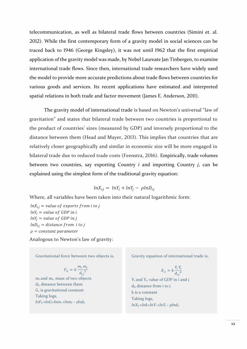
The gravity model of international trade is based on Newton’s universal “law of
gravitation” and states that bilateral trade between two countries is proportional to
the product of countries’ sizes (measured by GDP) and inversely proportional to the
distance between them (Head and Mayer, 2013). This implies that countries that are
relatively closer geographically and similar in economic size will be more engaged in
bilateral trade due to reduced trade costs (Feenstra, 2016). Empirically, trade volumes
between two countries, say exporting Country i and importing Country j, can be
explained using the simplest form of the traditional gravity equation:
𝑙𝑛𝑋𝑖𝑗 = 𝑙𝑛𝑌𝑖 + 𝑙𝑛𝑌𝑗 − 𝜌𝑙𝑛𝐷𝑖𝑗
Where, all variables have been taken into their natural logarithmic form:
𝑙𝑛𝑋𝑖𝑗 = 𝑣𝑎𝑙𝑢𝑒 𝑜𝑓 𝑒𝑥𝑝𝑜𝑟𝑡𝑠 𝑓𝑟𝑜𝑚 𝑖 𝑡𝑜 𝑗
𝑙𝑛𝑌𝑖 = 𝑣𝑎𝑙𝑢𝑒 𝑜𝑓 𝐺𝐷𝑃 𝑖𝑛 𝑖
𝑙𝑛𝑌𝑗 = 𝑣𝑎𝑙𝑢𝑒 𝑜𝑓 𝐺𝐷𝑃 𝑖𝑛 𝑗
𝑙𝑛𝐷𝑖𝑗 = 𝑑𝑖𝑠𝑡𝑎𝑛𝑐𝑒 𝑓𝑟𝑜𝑚 𝑖 𝑡𝑜 𝑗
𝜌 = 𝑐𝑜𝑛𝑠𝑡𝑎𝑛𝑡 𝑝𝑎𝑟𝑎𝑚𝑒𝑡𝑒𝑟
Analogous to Newton’s law of gravity:
Gravity equation of international trade is,
𝑋𝑖𝑗 = 𝑘𝑌𝑖 𝑌𝑗
𝑑𝑖𝑗𝜌
Yi and Yj, value of GDP in i and j
dij, distance from i to j
k is a constant
Taking logs,
lnXij =lnk+lnYi +lnYj – plndij
Gravitational force between two objects is,
𝐹𝑖𝑗 = 𝐺𝑚𝑖 𝑚𝑗
𝑑𝑖𝑗2
mi and mj, mass of two objects
dij, distance between them
G, is gravitational constant
Taking logs,
lnFij =lnG+lnmi +lnmj – 2lndij

13
The term “gravity equation” refers to the specification of the determinants of
bilateral trade flows. Theoretically, several studies have modelled the gravity equation,
including Krugman (1980), Eaton and Kortum (2002), and Melitz (2003). Generally,
across many applications, the estimated coefficients on “mass” variables (represented
by GDP) cluster around value 1, while the distance coefficients cluster close to –1. Most
observations are close to the fitted line, capturing about 80-90% of the variation in
trade flows. The fit of the traditional gravity model improves when other proxies for
trade frictions are incorporated, such as geographical borders and common language
effects. An interesting study by McCallum (1995) called Border Puzzle found intra-
national trade is much higher than inter-national trade. He compared trade flows
between Canadian provinces and across the U.S. and Canadian border and,
surprisingly, trade between Canadian provinces was 22% higher.
As gravity models continued to be tested empirically, the traditional model
received considerable criticism. The main critique was its lack of theoretical
foundation. However, numerous studies have attempted to bridge this theoretical gap
and present more functional forms of the gravity model, notably Anderson (1979),
Bergstrand (1985, 1990), and, more recently, Head and Mayer (2013). By 2004, gravity
models’ connection to economic theory became well-established (James E. Anderson,
2011) and they began appearing in economics textbooks (Feenstra, 2004).
The 1990s witnessed an ongoing debate about reshaping the specification of
gravity models into a better functional form. A more elaborated theoretical framework
was presented by Anderson and Van Wincoop (2003), which has been well
appreciated in the applied literature. Their gravity methodology was also presented
as a solution to McCallum’s border puzzle. However, despite its popularity, this new
model also had its assumptions and limitations. Nevertheless, recent debates on
gravity are about estimation techniques. Traditional literature employed ordinary
least squares (OLS) methods to estimate the gravity equation. However, recent
literature, for example Redding and Venables (2004), has suggested including
importer and exporter fixed effects to capture multilateral resistance terms and to
control for omitted variables. Silva and Tenryro (2006) contributed further by

14
suggesting using the Poisson method to treat zeroes in the trade data. Economic
literature shows that gravity models has also been successfully applied to estimate the
impact of a common (official or spoken) language on bilateral trade. Egger and
Lassmann (2012) found that, on average, a common or spoken language between
countries directly increases trade flows by 40%.
More recently, using gravity equations to estimate migration flows has become
quite popular among researchers and economists. We now turn to the gravity model
of international migration, founded in the groundbreaking work of Ravenstein (1889)
who used the gravity model to study migration patterns in the UK. Years later,
Steward (1941) specified aggregate models of migration, which may be considered as
modified versions of gravity models. These models are “gravity-like” because they
hypothesize that migration is directly related to population size in the origin and
destination regions and inversely related to distance. The same modeling techniques
used in the trade literature can also be applied to migration flows (Anderson, 2011)
and other interactions. Again, adapting from Newton’s law of gravity, the functional
form of gravity equation for migration can be presented as:
𝑇𝑖𝑗 = 𝐺𝑚𝑖
𝛼 𝑛𝑗
𝛽
𝑓(𝑑𝑖𝑗)
Where, Tij is the number of individuals (or immigrant rate) that move from location i
to location j per source population, per unit of time, and is expressed as being
proportional to some characteristics of the source (mi) and destination (nj) locations,
like population size, while at the same time declining with the distance dij between
them. 𝛼 , 𝛽 are two adjustable exponential coefficients.
Overall, we find that academic literature provides a significant evidence to
nominate language as the best candidate for representation of cultural characteristics
in a gravity model setting, either for trade or migration.

15
3. Empirical Model
This section describes the empirical strategy used to model how linguistic
proximity affects international migration flows to a particular destination, as well as how
linguistic proximity may influence bilateral trade. This section also presents the
econometric methodology adopted to estimate our empirical gravity-based models.
3.1 Estimating Equations
Previous empirical findings and theoretical background, as discussed in Section
2, have shown that we cannot fully understand global trade and migration by relying on
economic variables alone, without explicitly accounting for cultural factors as well. In
terms of statistical interpretation, the most realistic proxy for culture is language. In the
context of migration, language skills are a key variable in explaining immigrants’
disparities in educational attainment, earnings, and social outcomes. Likewise, language
(and cultural) barriers create trade costs that can stifle international trade. However, the
way in which previous studies accounted for language has been limited to controlling
for sharing a common language through a binary variable. A binary variable may not
capture the full impact of language on bilateral trade and migration. Therefore, in this
thesis, we employ the elaborated index of linguistic proximity developed by Adserà and
Pytliková (2015), which has gained significant popularity in academic world since it was
first introduced.
Our objective is to estimate the impact of linguistic proximity as a driver of
migration and trade simultaneously, using the same independent variables. Our
approach is to study these models in parallel. To the best of our knowledge, no previous
academic work has taken our specific approach to answering this question. Our
approach enables us to conduct a parallel comparative analysis of two apparently
different models. Furthermore, we are interested in examining how gravity variables
(such as countries’ geographical distance and economic size) interact with linguistic
proximity to control its impact on bilateral flows of goods and people. We would also

16
like to examine whether linguistic distance and geographical distance impact migration
and trade with the same magnitude.
a. Migration Model
For simplicity, we employ a basic gravity model, which allows for straightforward
interpretation of the coefficients. In addition, we use panel regressions with fixed effects
to control for omitted variables and unobserved characteristics. We opted for a log-
linear model using the count method to fit the non-negative dependent variable. In this
way, estimation results will not be biased. A common problem in estimating gravity
models is that the data often contains many observations with value zero, which we
resolve by adding 1 to each observation of immigration flows. Thus, when taking the
logarithm, we do not discard zero observations. Our migration model based on gravity
methodology using fixed effects reads as:
𝐥 𝐧(𝑴𝒊𝒈𝒓𝒂𝒕𝒊𝒐𝒏𝒊𝒋𝒕) = 𝜷𝟎 + 𝜷𝟏𝐥 𝐧(𝑮𝑫𝑷𝒊𝒕−𝟏𝒑𝒄) + 𝜷𝟐𝐥 𝐧(𝑮𝑫𝑷𝒋𝒕−𝟏𝒑𝒄) +
𝜷𝟑𝐥 𝐧(𝑮𝑫𝑷𝒊𝒕−𝟏) + 𝜷𝟒𝐥 𝐧(𝑮𝑫𝑷𝒋𝒕−𝟏) + 𝜷𝟓𝐥 𝐧(𝑫𝒊𝒋) + 𝜷𝟔 𝑳𝒊𝒋 + 𝜹𝒊 + 𝜹𝒋 + 𝜽𝒕 + 𝜺𝒊𝒋𝒕 (1)
The key variables in equation (1) are:
Migrationijt, denotes the gross flow of migrants from source country i to destination
country j (in other words, the number of emigrants from country i who immigrate to
country j) at time t, where i = 1, 2 …. 223; j = 1,2 …. 30; and t = 27 years;
GDPit-1pc, denotes GDP per capita (in current US $) in source country i, t-1 is the
economic indicator to capture development effects (lagged);
GDPjt-1pc, denotes GDP per capita (in current US $) in destination country j, t-1 is the
economic indicator to capture development effects (lagged);
GDPit-1, denotes GDP (in current US $) of source country i at time t-1 to capture
economic size and provide country-specific characteristics;
GDPjt-1, denotes GDP (in current US $) of destination country j at time t-1 to capture
economic size and provide country-specific characteristics;
Dij, denotes the geographic distance between the capital cities of source country i
and destination country j in kilometers;

17
Lij, denotes the Linguistic Proximity Index, which measures the linguistic closeness
between country pairs;
Ꝋt, denotes year dummies to control for common idiosyncratic shocks over the time
period and robust errors, clustered at each source-destination country pair;
δi δj, denotes country of origin and country of destination fixed effects separately to
capture unobserved characteristics;
Ꞓijt, denotes the idiosyncratic error term.
All variables used in the estimations, except for dummy variables and the
Linguistic Proximity Index, are expressed in their natural logarithm form. This
specification has the added advantage of easy interpretation of the estimated parameters
as being relative elasticities – in other words, by how much do migration flows between
a given source-destination country pair increase when GDP of either country increases
by 10%, while holding all other variables constant.
The relative differences in economic development and size between origin and
destination countries are lagged by one period to account for the information available
to a potential migrant at the time of deciding whether or not to migrate. Lagging the
economic explanatory variables and treating them as predetermined with respect to
current migration flows reduces the risk of reverse causality in our model.
The specification in equation (1) assumes that migration inflows to a particular
destination are driven by differences in economic development, economic size between
source and destination countries, and the costs of migration in the form of language
barriers and geographical distance. We expect economic theory to hold true that
migration decisions involve a comparison of country- or region- specific variables. High
wages or income levels in the source country and high migration costs discourage
emigration. GDP per capita is normally used as a proxy for wages or income, while the
physical and cultural distance between two countries acts as a proxy for migration costs.
The existing literature confirms that the propensity to migrate decreases with higher
levels of GDP per capita in the source country and larger distances between the source
country and destination country, as the economic incentives to migrate to other
countries decline. A potential emigrant takes these variables into account when

18
choosing to reside in the country where his utility is maximized among the possible
destinations. To control for the economic size of countries and to provide their specific
characteristics, we also include GDP at both source and destination countries. We
assume that the propensity to migrate between a specific country pair depends in part
on economic size, as countries with relatively higher GDP or that are more developed
tend to attract more immigrants.
Beyond the economic dimension, we also expect costs associated with migration
to increase with the geographical, cultural, and linguistic distance between countries.
Variable Lij, includes measures of linguistic proximity between countries (details in
subsequent Section 4 on data construction) and tests our hypothesis: Whether larger
language barriers increase migration costs for a potential migrant by posing barriers to
skills transfer and integration in the receiving country. We use log-distance in
kilometers between the capital cities of sending and receiving countries to control for
the effect of geographical distance. Finally, our model includes year dummies to control
for common idiosyncratic shocks over the time period. Our model also contains country
of destination and country of origin fixed effects separately to capture unobserved
characteristics, for example immigration policy in destination country, credit market
constraints at origin as well as climate, openness towards foreigners or culture in each
country, networks of family and friends, and the population from the same origin
already living the destination country, among other things. Meanwhile, the country
fixed effects terms mitigate the risk of omitted variable bias by controlling for any
unobserved permanent differences between countries.
b. Trade Model
In parallel to the migration model described above, we estimate trade flows using
a modified gravity model with fixed effects on panel data. Our basic model takes the
form of:
𝐥𝐧(𝑻𝒓𝒂𝒅𝒆𝒊𝒋𝒕) = 𝜷𝟎 + 𝜷𝟏 𝐥𝐧(𝑮𝑫𝑷𝒊𝒕−𝟏𝒑𝒄) + 𝜷𝟐 𝐥𝐧(𝑮𝑫𝑷𝒋𝒕−𝟏𝒑𝒄) + 𝜷𝟑 𝐥𝐧(𝑮𝑫𝑷𝒊𝒕−𝟏) +
𝜷𝟒 𝐥𝐧(𝑮𝑫𝑷𝒋𝒕−𝟏) + 𝜷𝟓 𝐥𝐧(𝑫𝒊𝒋) + 𝜷𝟔 𝑳𝒊𝒋 + 𝜹𝒊 + 𝜹𝒋 + 𝜽𝒕 + 𝜺𝒊𝒋𝒕 (2)
The dependent variable in equation (2) is Tradeijt,, which denotes gross trade flows from

19
exporting country i (akin to “source country” in the migration model) to importing
country j (akin to “destination country”) at time t. It is worth noting that the trade data,
collected from the Direction of Trade Statistics (DOTS), often reports two different
values for the same flow from Country A to B, due to differences in how Country A
reports its imports from Country B versus how Country B reports its exports to Country
A. Some studies suggest taking the average of these two values. This is to say that a trade
flow could be either an export or an import, depending on which country is reporting
the exchange. In addition, trade data is recorded in millions of dollars with 1 or 2 decimal
places, which can give rise to erroneous zero values, while actual trade is not zero. Many
missing observations are substituted with zeroes. Structured zeros are better treated as
missing observations rather than true zeroes.
The independent variables in equation (2) are same as those in equation (1), but
they work in a different fashion. As before, all variables used in the estimation, except
dummy variables and the Linguistic Proximity Index, are expressed in natural logarithms.
The zeroes issues in the data is treated by adding one to each observation of trade flows
so that taking the logarithm does not discard zero observations. We predict trade flows
using fixed effect regressions to account for unobserved variables within the data. We
also include the GDP of both exporting and importing country since these variables are
assumed to be correlated with the unobservable effects. We also use year dummies and
country-fixed effects in our estimation to control for heterogeneity within the model.
Using fixed effects mitigates omitted variable bias in the panel data arising from
unobserved differences across entities (countries i and j) that do not change over time.
Alternatively, omitted variable bias could be due to differences that affect all countries
in the same way, but that vary over time. We address this by lagging economic
explanatory variables and treat them as predetermined with respect to current trade
flows to reduce the risks of reverse causality in our model.
Our empirical gravity model in equation (2) estimates the determinants of
bilateral trade. These are driven by differences in the economic size of trading countries
and trade costs. We expect exports to rise proportionally with the economic size of the
destination country and imports to rise in proportion to the size of source economy.

20
Empirically, bilateral trade patterns between two countries are proportional to their
GDPs and inversely proportional to the distance between them. As previously discussed,
cultural proximity may influence bilateral trade through both preferences and trade
costs. Two culturally close countries may trade a lot because they have strong tastes for
each other’s products and/or because trade costs are relatively low. Sharing a common
language is an important symmetric component of cultural proximity, as are religion
and ethnicity. In this empirical bilateral trade flow model, we may attempt to
disentangle the trade cost channel (i.e. physical distance) from the preference channel
of cultural proximity (i.e. linguistic distance) to estimate whether linguistic distance and
geographical distance have a similar impact on trade.
3.2 Estimation Methodology for Gravity Equations
We now turn to the econometric methods used to estimate the standard gravity
model of migration and trade.
a. The Ordinary Least Squares (OLS) Estimators
Ordinary Least Squares (OLS) is the most widely-practiced method to analyze
data. It has become the starting point for regression analysis, particularly in social
sciences. The OLS estimation follows the assumptions of the classical linear regression
model. The regression coefficients predict the estimated regression line as closely as
possible to the observed data. OLS is the best application to study the econometric
relation of bilateral flows with respect to GDP and distance. Furthermore, OLS has been
the most practical tool to estimate traditional gravity models. Using OLS for gravity
model estimates requires the following conditions to hold:
The other factors contained in gravity error term (𝜺𝒊𝒋𝒕) have conditional mean zero
and are uncorrelated with each of the explanatory variables.
The errors are independently drawn from a normal distribution with a constant
variance (homoscedasticity assumption).
None of the explanatory variable is a linear combination of another explanatory
variable (no multicollinearity).

21
If all three are conditions met, the OLS estimates are consistent, unbiased, and
efficient. In our estimation, there are unobserved characteristics that might affect
migrant flows and trade volumes, which means that the homoscedastic error terms
assumption is very strong and may not necessarily hold, thus making OLS estimates
inefficient. The OLS presumes that error terms in trade data are independent for each
country-pair such that country i exports to country j are independent of imports to i
from j. This assumption would be violated in practice, if a country is producing and
exporting a product that is being used as an input in the production process of another
country. Thus, gravity error terms are correlated with each other and its OLS estimates
are inefficient, but this does not affect consistency and unbiasedness. As we are using a
log-linear model, there is a risk to efficiency due to missing information in the presence
of zero valued observations. However, we resolve this problem by adding 1 to each
observation of trade flows and migration flows. We use year dummies (a time factor t)
which control for common idiosyncratic shocks over time and to capture the influence
of aggregate trends which might affect the explanatory variable(s). This is important, as
time-variant variables are falsely related to aggregate trend variables like economic
development, inflation, and population growth. This is more probable in the case of
panel data. Conventional OLS regression serves as a baseline reference point in our
results, which is then compared to alternative specifications with country-fixed effects.
b. The Fixed Effects Regression
Estimates from OLS have a tendency to produce biased results due to their
inability to take unobserved variables into account, which are instead captured by the
error term. In contrast, fixed effects regressions on panel data control for omitted
variables if the omitted variables vary across entities but are constant over time.
In panel data, the regression error can be correlated over time within an entity.
As with heteroscedasticity, this correlation does not introduce bias into the fixed effect
estimator, but it does affect the variance of the fixed effects estimator. By using fixed
effects regressions, we control for omitted variables in the traditional gravity model. This
does not require the assumption of symmetrical trade costs. We take country-specific
fixed effects into account by creating dummies for exporting and importing countries.

22
This way, we assume an unobserved heterogeneous component as being constant over
time within each specific country. Potential unobserved sources of heterogeneity in the
trade model are, for example, trade policies, regional trade agreements (RTAs), or
treaties signed between countries affect trade volumes, while in the migration model,
these sources could be the stock of immigrants already at destination, migration policy,
or cultural proximity affect bilateral migration flows. Likewise, fixed effects in migration
models means that dummy variables equal to unity each time a particular country
appears in the dataset. The standard errors in fixed effect regressions are called clustered
standard errors and are robust to both heteroscedasticity and correlation over time
within an entity.
Fixed effects also come with some issues. Variables that only vary in the same
dimensions as the fixed effects will become perfectly collinear and the regression will
drop them. At the same time, fixed effects regressions do not solve endogeneity bias
because unobserved variables might vary in another dimension than the fixed effects.
Hence, absence of omitted variable bias is not fully guaranteed. Endogeneity occurs
when an explanatory variable is correlated with the error term.
Another inadequacy of using fixed effects estimation is that it cannot handle zeroes
in the dependent variable, and instead treats them as missing. This is similar to the case
with trade flows, which consists of structured zeros due to missing observation or ‘false’
zero values. However, as discussed earlier, migration and trade data sets are partially
treated for zero issues by adding 1 to each observation of migration flows and trade flows.
Thus, the log-linear migration model is developed using the count method to fit the
non-negative dependent variable. This way, estimation results are not biased.
c. The Poisson Fixed Effect Regression
An alternative way to address zeroes in the data is to use a Poisson regression, which
also accounts for heteroscedasticity. As a robustness check and alternative method to
estimate gravity models, I also employ a Poisson regression, which is consistent with
fixed effects. These results are discussed separately in the robustness section.

23
4. Data Description and Structure
This section describes the data and variables that used in the empirical analysis.
It also presents summary statistics for the population under study. Variables are defined
in the Appendix.
4.1 Data Sources
To analyze and estimate the two empirical models specified in Section 3, we
require information on bilateral flows (for both migration and trade) and a measure of
linguistic proximity that, along with gravity variables, can establish a meaningful and
correlative relationship. This data was obtained through two different sources to fit both
bilateral flow gravity models.
a. International Migration Data
We use a dataset adapted from Adserà and Pytliková (2015) containing
information on migration flows from 223 source countries to 30 OECD destination
countries over the period 1980-2010. This data was primarily collected through national
statistical offices in OECD countries, and supplemented with data from the OECD
International Migration Database. This is a comprehensive dataset with respect to
destination countries, origin countries, and time. The dataset is quite extensive with
over 100 variables. In addition to the variables available directly, a number of other
variables related to gravity and that impact migration patterns were generated from
existing variables. OECD countries are the most reliable source of migration data. The
list of variables used in the analysis and their definitions is found in Table A.2 in the
Appendix section.
Figure 4 below illustrates the migration inflow at OECD countries from various
host countries around the world during the period of almost 30 years. We have selected
8 countries from our data of 30 OECD countries to roughly cover each region, also the
information on each of these countries is mostly available, thus making our panel
somewhat balanced. From the visualization of stacked countries, we find that the USA

24
is receiving bulk of immigrants with fluctuations over some periods. The USA is getting
steadily increasing number of migrants over years until they reaches at peak during
1990s. Australia and Canada have relatively stable flow, with growing number of
migrants at an increasing rate as compared to rest of the countries. Meanwhile, Germany
is also receiving a significant surge of migrants.
Figure 4 Migration Flows to selected OECD Countries from all world, 1980-2006
Source: Author’s tabulation based on data on migration flows
b. Trade Data
In addition to migration data, we also used a gravity dataset from a geographical
database owned by CEPII, a French research center in international economics that
produces research, analyses, and databases on the world economy. This dataset includes
the variables and economic indicators commonly used in gravity models. For my analysis
of trade flows, I am interested in data on the GDP of both destination and source
countries. This dataset contains complete information for all pairs of countries (in total
224) from the period 1948–2006. Data on GDP and population size were obtained from
the World Bank Development Indicators (WDI). CEPII is considered as the most
accurate data on trade flows. The data is collected from the Direction of Trade Statistics
(DOTS), which often reports two different values for the same trade flow between two

25
countries, as discussed in Section 3. Some of the new variables were generated from the
data to better control the results. Variable details and definitions are listed in the
Appendix.
Figure 5 below illustrates the trade flows at OECD countries from various host
countries around the world during the period of almost 30 years. We have selected 8
countries from our data of countries as sample to broadly cover each geographical region
for OECD, also the available information on each of these countries is complete with no
missing information, so our panel for trade data is balanced. From the visualization of
overlaid countries, we can see that all countries have an increasing trend in trade. The
USA is the biggest market in terms of trade volumes. Japan and Germany follow the
almost same pattern, while Canada is relatively stable in its trade business with
increasing rate.
Figure 5 Trade Flows to selected OECD Countries from all world, 1980-2006
Source: Author’s tabulation based on data on trade flows
c. Linguistic Distance Measure
We primarily used three different indices of linguistic distance, namely:
i. The Linguistic Proximity Index (newly constructed), based on information
from Ethnologue;

26
ii. The Levenshtein Distance, developed by the Max Planck Institute for
Evolutionary Anthropology; and
iii. The Dyen Linguistic Proximity Measure proposed by Dyen et al. (1992).
Most previous studies include a simple dummy for whether two countries chare
a common language, which may not capture the true impact of language. We instead
use the Linguistic Proximity Index (LPI), used only in a couple of other studies to date.
Compared to a dummy variable, this index is more inclusive, provides a better-adjusted
and smoother indicator of proximity, and is quantifiable. The index ranges from 0 to 1
depending on how many levels of linguistic family tree the languages of the destination
and source countries share. Prior to constructing the index, a set of increasing weights
are defined as explained by Adserà and Pytliková (2015) as follows:
The first [weight] equal to 0.1 if the two languages are related at the most
aggregated linguistic level; the second equal to 0.15 if two languages belong to the
same second linguistic tree level; the third equal to 0.20 if two languages belong to
the same third linguistic tree level; and the fourth equal to 0.25 if both languages
belong to the same fourth level of linguistic tree family.
If two languages are identical, then the Linguistic Proximity Index takes value 1.
Otherwise, for languages that are different, the Linguistic Proximity Index is constructed
as the sum of the above four weights to capture the maximum number of shared
linguistic family tree’s branches.
Index = 0} if two languages do not belong to any common language family
Index = 1} if two countries have a common language
Thus, the Linguistic Proximity Index equals 0.1 if two languages are only related at
the most aggregated level of the linguistic; 0.25 if two languages belong to the same first
and second linguistic tree level; 0.45 if two languages share up to the third linguistic tree
level; and 0.7 if both languages share the first four levels. A good example of the latter
case are Scandinavian languages (Danish, Norwegian, and Swedish). My analysis
includes only first official language in each country pair, which is strong enough to
capture the effects of linguistic proximity in our hypotheses under study.

27
However, the visualization below presents a detailed information about the
distribution of migration flows by the linguistic tree level the source and destination
country share. It covers all country-pairs, over the period 1980-2006 with individual
representation of first official, all official & main and major languages.
Figure 6 Migration Flows by Linguistic Proximity Index OECD, 1980-2006
Source: Author’s adaptation7 based on Data on Migration Flows
During the period of 1980-2006, there were almost 110 million people migrating
to another OECD country: among them about 14.6 million people migrated to countries
that share the same first official language and about 40 million people migrated to
countries whose first official languages did not have any level in common with that of
their country of origin. The largest proportion of migrants almost 44 million, migrated
to countries whose languages share only the most aggregate linguistic tree family and
about 1.6, 6.9 and 2.1 million to countries sharing the second, third and fourth level of
linguistic tree respectively. The overall pattern is not different in terms of migration by
major language spoken, though more migrants are moving to countries with major
languages very distant. When all official and main languages are considered, the flows
to destinations with a common language are strikingly higher. This is of course partially
due to the fact that countries shared a common colonial past.
7 Adserà and Pytliková (2015)

28
By adopting the same functionality as above, we used trade data and derived the
distribution of trade flows by the linguistic tree level the exporting and importing
country share. From figure 7 below, we find that the overall pattern of distribution is
interestingly quite comparable to that of migration flows’. Based on our data, there is
total trade of about 100 trillion US dollars between OECD and all world countries during
1980-2006. Out of this, about 10.6 trillion US dollars trade was carried out between
those trading partners that share the same first official language and about 30.3 trillion
US dollars’ worth of business was conducted between countries whose first official
languages did not have any level in common.
Figure 7 Trade Flows by Linguistic Proximity Index OECD, 1980-2006
Source: Author’s tabulation based on data on trade flows
When all official and main languages are considered, the trade flows to OECD
countries with a common language are strikingly higher, similar to migration patterns.
4.2 Data Merging
To produce a single dataset for estimation purposes, we have merged the trade
and migration data, then extracted the variables of interest. Both datasets include
information about source and destination countries and the corresponding observation
year. This information served as the basis for merging. Countries were listed by their
standard ISO 3-letter codes. In addition, a specific numeric code for each country was

29
combined to produce a unique ID for each country-pair (i.e. destination country
numeric code ×1000 + source country numeric code). These IDs enabled us to deal with
the string nature of the variable country name or its 3-letter ISO code. We discovered
that the CEPII data incorporated a longer observation period than did the migration
dataset. The migration data covered the period 1980–2010 with 215,040 observations,
while CEPII covered the period 1948–2006 with 1,204,671 observations. Almost 65% of
migration data was merged with CEPII data, while the remaining data was dropped.
However, most of the observation recorded for recent years overlapped. Following the
merge, our final dataset contained 137,472 observations over a span of 27 years, which is
a considerably good number.
4.3 Dependent Variable(s)
We want to study two relationships: (1) The effect of language proximity on
migration decisions in parallel to (2) the effect of language proximity on trade volumes
between any two pairs of countries. Therefore, Migration Flows and Trade Flows are our
two dependent variables in their respective gravity models.
4.4 Summary Statistics
Key characteristics of the dependent and control variables for our population
under study are summarized in Table 1 below. The table shows the data for the period
1948-2010 comprising of 1,282,239 observations for a 62-year period.
Turning first to our migration data, gross migration flows from source country i
to destination country j (where i = 1,2,…223 source countries and j = 1,2,… 30 destination
countries) is our main dependent variable for one of the models, in which we want to
study the relevance of linguistic proximity between origin and destination countries in
the decision to migrate.
Turning next to our trade data, gross trade flows from exporting country i to
importing country j is the dependent variable to study the significance of language
proximity in defining international trade patterns. Country-pairs are same for both
models.
30
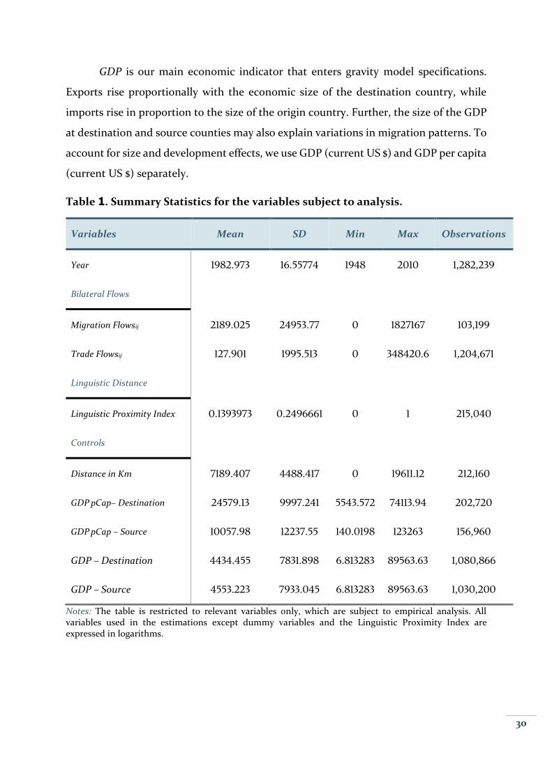
GDP is our main economic indicator that enters gravity model specifications.
Exports rise proportionally with the economic size of the destination country, while
imports rise in proportion to the size of the origin country. Further, the size of the GDP
at destination and source counties may also explain variations in migration patterns. To
account for size and development effects, we use GDP (current US $) and GDP per capita
(current US $) separately.
Table 1. Summary Statistics for the variables subject to analysis.
Variables Mean SD Min Max Observations
Year 1982.973 16.55774 1948 2010 1,282,239
Bilateral Flows
Migration Flowsij 2189.025 24953.77 0 1827167 103,199
Trade Flowsij 127.901 1995.513 0 348420.6 1,204,671
Linguistic Distance
Linguistic Proximity Index 0.1393973 0.2496661 0 1 215,040
Controls
Distance in Km 7189.407 4488.417 0 19611.12 212,160
GDP pCap– Destination 24579.13 9997.241 5543.572 74113.94 202,720
GDP pCap – Source 10057.98 12237.55 140.0198 123263 156,960
GDP – Destination 4434.455 7831.898 6.813283 89563.63 1,080,866
GDP – Source 4553.223 7933.045 6.813283 89563.63 1,030,200
Notes: The table is restricted to relevant variables only, which are subject to empirical analysis. All variables used in the estimations except dummy variables and the Linguistic Proximity Index are expressed in logarithms.

31
Distance (in kilometers) represents the distance between the capital cities of
sending and receiving countries. We expect both migration and trade to decrease with
as the physical distance between countries increases.
The Linguistic Proximity Index ranges from 0 to 1 depending on the number of
linguistic family tree levels shared by the first official languages of the destination and
source countries. Additional summary statistics for the full set of variables and their
description employed in empirical analyses and for robustness may found in Appendix
table A.1.
Based on our gravity dataset, we can also demonstrate the overall trend in
migration and trade patterns for OECD countries during the span of 27 years, from
2006-1980 through figure 8, below:
Figure 8 Development in Migration and Trade Flows for OECD countries 1980-2006
As visualized, we find that trade is growing smoothly at an increasing rate, with
not very sharp spikes during the period, while migration flows though increasing but
experiencing much fluctuations during the same period.

32
5. Empirical Results
This section presents the main findings of our econometric models by employing
a series of regression analyses, followed by a discussion. We also investigate the
usefulness of the gravity model for trade and migration, as well as discuss the robustness
of our models and the implications of our results.
5.1 Main Results
Based on the econometric model developed and discussed in Section 3, we begin
by using a conventional ordinary least squares (OLS) approach. Afterwards, we run OLS
regressions with country- and time-fixed effects. This is a common approach when
working with panel data, as it controls for unobserved individual heterogeneity, or
unobserved characteristics that vary by country or by year. In addition, we use robust
standard errors to control for heterogeneity in the error term, which also means that our
standard errors are heteroscedastically consistent.
In what follows, we first present individual results for each model separately, and
later present a comparison of the models.
a. Migration Model Estimation Results
Beginning with the migration model, three different estimation results of the log-
linear model introduced in Section 3 through equation (1) are tabulated below in Table
2. The dependent variable is the log of migration flows. All three regressions include
year dummies to control for time-fixed effects. However, only one of the regressions
controls for country-fixed effects by incorporating country-specific fixed effects for each
source and destination country over time.
From Table 2 below, we can determine the effect of linguistic proximity and basic
gravity variables on migration flows. The first regression in Column (1) provides
coefficient estimates for a simple OLS regression where the only regressor is the

33
Linguistic Proximity Index. It gives statistically significant results for a sample
encompassing over 103,000 observations.
Table 2. Effect of Language Proximity and Gravity Variables on Migration Flows
(1) (2) (3)
Regressors OLS OLS Fixed Effects
Linguistic Proximity Index 1.592*** 1.673*** 1.112***
(0.174) (0.116) (0.136)
Ln GDP pCap _Dest_t-1 0.265*** -2.345***
(0.0328) (0.327)
Ln GDP pCap _Orig_t-1 -0.353*** -0.129
(0.0199) (0.158)
Ln Distance in km -0.650*** -1.082***
(0.0301) (0.0501)
Ln GDP_Dest_t-1 0.898*** 2.714***
(0.0178) (0.330)
Ln GDP_Orig_t-1 0.696*** -0.158
(0.0141) (0.187)
Constant 3.101*** -7.449*** 9.423***
(0.0839) (0.459) (1.480)
Observations 103,199 73,359 73,359
R-squared 0.024 0.641 0.778
Country FE NO NO YES
Dependent Variable: Natural logarithm of migration flows between country i and j at time t. Robust standard errors are reported in parentheses. All models include year dummies. Regressions are controlled for country-specific FE for source and destination in the model of Fixed Effects. *** Statistically significant at the 1 % level p<0.01 ** Statistically significant at the 5 % level p<0.05 * Statistically significant at the 10 % level p<0.1
34
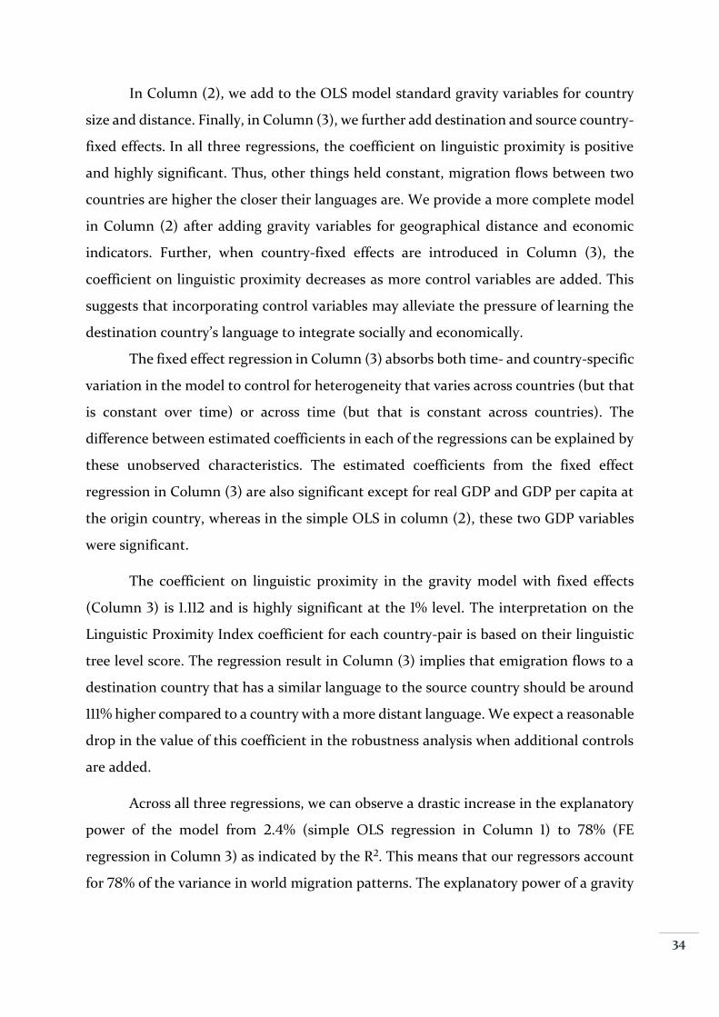
In Column (2), we add to the OLS model standard gravity variables for country
size and distance. Finally, in Column (3), we further add destination and source country-
fixed effects. In all three regressions, the coefficient on linguistic proximity is positive
and highly significant. Thus, other things held constant, migration flows between two
countries are higher the closer their languages are. We provide a more complete model
in Column (2) after adding gravity variables for geographical distance and economic
indicators. Further, when country-fixed effects are introduced in Column (3), the
coefficient on linguistic proximity decreases as more control variables are added. This
suggests that incorporating control variables may alleviate the pressure of learning the
destination country’s language to integrate socially and economically.
The fixed effect regression in Column (3) absorbs both time- and country-specific
variation in the model to control for heterogeneity that varies across countries (but that
is constant over time) or across time (but that is constant across countries). The
difference between estimated coefficients in each of the regressions can be explained by
these unobserved characteristics. The estimated coefficients from the fixed effect
regression in Column (3) are also significant except for real GDP and GDP per capita at
the origin country, whereas in the simple OLS in column (2), these two GDP variables
were significant.
The coefficient on linguistic proximity in the gravity model with fixed effects
(Column 3) is 1.112 and is highly significant at the 1% level. The interpretation on the
Linguistic Proximity Index coefficient for each country-pair is based on their linguistic
tree level score. The regression result in Column (3) implies that emigration flows to a
destination country that has a similar language to the source country should be around
111% higher compared to a country with a more distant language. We expect a reasonable
drop in the value of this coefficient in the robustness analysis when additional controls
are added.
Across all three regressions, we can observe a drastic increase in the explanatory
power of the model from 2.4% (simple OLS regression in Column 1) to 78% (FE
regression in Column 3) as indicated by the R2. This means that our regressors account
for 78% of the variance in world migration patterns. The explanatory power of a gravity

35
model generally ranges from 60 to 80% (Feenstra, 2016). This increase in R2 can also be
explained by the addition of country- and year-fixed effects to absorb much of the
heterogeneity. In contrast, the R2 value of 2.4% from the simple OLS regression in
Column 1 indicates that there remains much unobserved heterogeneity not accounted
for by the model.
The estimated coefficient on GDP per capita in Column (2) is significant and
positive for the destination country, but significant and negative for the source country.
These signs correspond to our expectation that migration flows tend to go from
relatively poorer to relatively richer countries. A 10% increase in a destination country’s
GDP per capita results in a 2.6% increase in immigration. The negative sign of GDP per
capita in source country indicates that potential emigrants have less incentive to migrate
as economic opportunities in their own country of origin grow. In contrast to Column
(2), the fixed effects model in Column (3) predicts that migration flows are inversely
related to GDP per capita of the destination country. This is an unexpected result that
goes against economic theory and may be an indication that GDP per capita in the
destination country is not only correlated to the response variable but also to other
predictors in the model. Real GDP at destination has a positive and significant impact
on migration flows in Column (3), where a 10% increase in the GDP of the destination
country is associated with a 27% increase in immigration flow to that country. This is
also in line with economic theory that relatively larger and economically stronger
countries attract more immigrants, ceteris paribus, as prospective immigrants tend to
migrate looking for better standards of living and job opportunities. Meanwhile, both
real GDP and GDP per capita in the origin country both in Column (2) and Column (3),
entering negatively and insignificantly in both regressions, albeit with small magnitudes.
This implies that GDP and GDP per capita at source is associated with an economically
and statistically insignificant decrease in migration flows.
Geographical distance is also an important determinant of migration. We expect
that shorter distances between countries are significantly associated with larger
migration flows. Therefore, to control for the effect of geographic distance, we include
a regressor for the logarithmic distance (in kilometers) between the capital cities of the

36
sending and receiving countries. The estimated coefficients in Columns (2) and (3) show
that distance has a statistically significant and negative impact on migration flows.
Specifically, in the Column (3) model, a 10% increase in the physical distance between
capital cities is associated with an almost 11% decrease in migration flows. Migration
costs increase when countries are further apart as transportation costs increase with
distance. It is also interesting to note that, in Column (3), linguistic distance and physical
distance have a similar impact (in terms of magnitude) on migration flows.
There are other factors that may affect migration flows but not included in our
model, such as the stock of migrants from the same country of origin already residing in
the destination country, unemployment constraints, social security systems, public
social expenditures, political stability, and employment rates. In the absence of such
variables, the coefficient on GDP may be biased. This raises the possibility of omitted
variable bias, which is addressed in the robustness analysis in the next section. However,
for our purposes, using standard gravity variables is sufficient to establish a causal
relationship with respect to migration. Furthermore, the interaction between the gravity
variables and linguistic proximity does not undermine the importance language as a
determinant of migration.
To summarize, we find that language proximity is an important determinant of
migration between two countries, even after controlling for gravity variables for
economic size and geographic distance. In our model, whether or not countries share a
common language affects immigration flows to a larger extent than does GDP, while
linguistic distance and geographical distance have almost the same impact on migration.
In short, the more similar the languages and the shorter the distance between two
countries, the greater the migration between them.
b. Trade Model Estimation Results
Turning now to the trade model, the same methodology used in the migration
analysis was applied to our augmented gravity model of trade to determine how
language proximity affects levels of trade between trading partners. From the log-linear
form of our trade model in equation (2), estimation results are tabulated in Table 3

37
below. As before, year dummies are included in all three regressions to control for time-
fixed effects.
Table 3. Effect of Linguistic Proximity and Gravity Variables on Trade Flows
(1) (2) (2)
Regressors OLS OLS Fixed Effects
Linguistic Proximity Index 0.924*** 0.619*** 0.418***
(0.155) (0.0662) (0.0686)
Ln GDP pCap _Dest_t-1 0.111*** -1.851***
(0.0225) (0.203)
Ln GDP pCap _Orig_t-1 0.147*** 1.097***
(0.0132) (0.0858)
Ln Distance in km -0.709*** -0.959***
(0.0200) (0.0299)
Ln GDP_Dest_t-1 0.698*** 2.225***
(0.0130) (0.212)
Ln GDP_Orig_t-1 0.743*** -0.617***
(0.00862) (0.0953)
Constant 2.322*** -7.861*** 1.857*
(0.0413) (0.293) (0.956)
Observations 137,472 123,880 123,880
R-squared 0.014 0.742 0.829
Country FE NO NO YES
Dependent Variable: Natural logarithm of trade flows between country i and j at time t. Robust standard errors are reported in parentheses. All models include year dummies. Regressions are controlled for country specific FE for each exporting & importing countries in the model of Fixed Effects. *** Statistically significant at the 1 % level p<0.01 ** Statistically significant at the 5 % level p<0.05 * Statistically significant at the 10 % level p<0.1

38
Table 3 presents a set of regression results for the effect of linguistic distance and
basic gravity variables on trade flows. Column (1) shows coefficient estimates for the
standard OLS regression where Linguistic Proximity Index is the only regressor. It gives
statistically significant results for the full sample under study, encompassing around
137,000 observations.
Column (2) adds standard gravity variables for economic size and geographic
distance, while Column (3), our model of interest, further incorporates country-fixed
effects to control country-specific characteristics for each exporting and importing
country that are constant over time
The coefficient on linguistic proximity is positive and highly significant in all
three specifications. Thus, other things being equal, we find that the volume of trade
between two countries is higher if their official languages are closer. These results hold
for aggregate exports and imports.
As expected, the coefficient on linguistic proximity decreases in magnitude as
more controls are added, from Column (1) to Column (2) to Column (3). The inclusion
of country-fixed effects regression in Column (3) shows that differences between
estimated coefficients across the three regressions is due in part to unobserved
characteristics. The coefficient on linguistic proximity in the gravity model setting with
fixed effects in Column (3) is 0.418, which is highly significant at 1% level. This implies
that trade flows between country pair i and j are around 42% higher when the countries
share a similar first official language, compared to if their languages are more distant.
The estimated coefficients on all the economic variables (i.e. GDP and GDP per
capita) in the OLS regression in Column (2) are statistically significant and positive, and
appear to substantiate economic theory. Trade between exporting and importing
countries increases with increases in their respective GDP level or GDP per capita levels.
For example, a 10% increase in the GDP of an exporting country (i.e. source country)
will boost its trade volumes by 7.4%. In the estimation results with fixed effects in
Column (3), we find that GDP and GDP per capita are significant both for destination
and source, but with opposing signs. The estimated coefficient on GDP per capita of the
importing country j has a statistically significant and negative effect on aggregate trade

39
values, suggesting that a 10% higher GDP per capita in importing country will decrease
trade volumes by 18.51%. This contrasts with macroeconomic theory, which suggests
that a country’s imports are positively affected by the country’s national income. We
also expect our results to be consistent with the economic theory that exports rise
proportionally with the economic size of the destination country and imports rise in
proportion to the size of the source economy. In our estimates, the GDP per capita of
the exporting country has a positive and significant effect: A 10% increase in the GDP
per capita of the exporting country (source) is associated with an increase in their
exports by around 11%, in other words we can say that imports at destination are
increasing. We also expect less developed countries tend to import more than they
export due to their lower capacities and underutilization of resources. To account for
the economic size of countries, we used real GDP (at current US $) for both exporting
and importing countries. The estimated coefficient shows that GDP for importing
country j is highly significant at the 1% level with a positive impact on trade flows. These
results strongly support the economic theory that trade increases proportionally with
the relative economic size of the countries, ceteris paribus. However, the GDP of the
exporting country i is significant and negative. Thus, a 10% increase in the GDP of the
exporting country is associated with an almost 6% decline in trade volume, while a 10%
increase in the GDP of the importing country implies an approximately 22% increase in
bilateral trade. The importing country’s GDP is relatable to trade theory whereby GDP
has a positive effect on trade, simply because economically larger countries tend to trade
more. This, in turn, means increased globalization and economic development.
Geographical distance is an integral part of gravity models and an important
determinant of trade patterns. We expect our empirical model to shows that bilateral
trade flows are inversely proportional to the distance between trading countries. Indeed,
the estimated coefficient on distance has a statistically significant and negative impact
on trade. Specifically, from Column (3), a 10% increase in the physical distance between
capital cities is associated with a decrease in aggregate trade volumes of almost 10%.
Additionally, we find that R2 equals 0.829 in the country-fixed effects regression
model of Column (3), indicating that our model explains 83% of the variance in world

40
trade flows. The increased absolute value of R2 as compared to the conventional OLS
regressions in Columns (1) and (2) demonstrates that controlling for country-fixed
effects captures much of the unobserved heterogeneity in the model.
Certainly, there are other economic and non-economic factors that contribute to
increased bilateral trade flows, such as trade policies, regional trade agreements (RTAs),
treaties signed by the member countries of multinational organizations like the WTO,
the EU or by a country’s neighbors. A common ethnic background or historical ties could
also favor trade between countries. The absence of these variables in our model could
induce omitted variable bias, whereby the coefficient on GDP is potentially biased. This
issue is discussed separately in the robustness analysis section. However, for our
objective of assessing the explicit role of language, using a standard gravity model is
sufficient to establish a causal relationship with respect to trade.
To summarize, we find that linguistic distance is an important determinant of
trade. Trade will be negatively impacted when two countries speak entirely distinct
languages. Linguistic distance and geographical distance both effect trade flows, but
with different magnitudes. Our model shows that trade between two countries in higher
they share a similar language, have higher levels of GDP, and have a shorter distance
between them.
5.2 Robustness
To test the robustness of our results, we include a set of additional controls. In
addition, we also estimate a Poisson regression with fixed effects. The results are
presented in Table 4 below. As an additional check, we also use alternative measures of
linguistic proximity, presented in Table 5.
To ensure comparability with our previous econometric results for migration and
trade, we include the same control variables as in our default econometric models while
running robustness checks. In addition to these control variables, we also include new
dummy variables. The coefficients on the dummy variables are interpreted as the mean
change in the dependent variable (i.e. either migration or trade flows) when the dummy
changes values from 0 to 1, holding all other variables constant.

41
First, we include a dummy variable for common colonial past, which controls for
whether countries share a common historical path or are tied to a common ethnic
background. The dummy assumes value 1 if there is common colonial past between
countries i and j, and 0 otherwise. A common history might decrease the cultural
distance between countries and increase the information available about the potential
destination country (Venturini, 2018 Discussion Paper). We also add a dummy to
control for whether a present colonial relationship still exists between countries. This
dummy takes the value 1 if country pairs are still in colonial relationship. As an
additional control for the effect of distance, we add neighboring country dummies,
which take the value of 1 if two countries are neighbors (i.e. they share a common border).
We may relate this to the Border Puzzle theory by McCallum (1995) stating that “intra-
national trade is much higher than inter-national trade”. We are interested in
identifying how sharing a common border can affect the patterns of trade, and do
people prefer to migrate in neighboring country.
Furthermore, we include a dummy taking value 1 if either the destination or
origin country is a member of the GATT or the WTO.
Finally, we also include a dummy which takes on 1 if there is a regional trade
agreement in force between countries i and j.
Empirically, the presence of migration networks – that is, a network of family
members, friends, or other people of the same origin already living in the host country
– is also expected to reduce migration costs (Massey et al., 1993; Munshi, 2003).
However, we do not include it in our robustness checks to avoid any possible
collinearity with GDP per capita through population from the source country. At the
same time, we also believe that country-fixed effects would capture the unobserved
characteristics of migration networks.
We ran a fixed effect regression and a Poisson regression, with year- and
country-specific fixed effects, with two different specifications (one for migration, the
other for trade), as displayed in Table 4. Columns (1) and (2) show the fixed effect
regression results for migration and trade, while Columns (3) and (4) show the
Poisson fixed effect regression results for migration and trade, respectively.

42
Table 4. Robustness Checks: Controlling with additional dummies and variables. Fixed Effect Regression and Poisson Estimation with fixed effect
(1) (2) (3) (4)
Regressors Fixed Effect Poisson
Dep. Var: Ln
(Migration
Flowsij)
Dep. Var: Ln
(Trade Flowsij)
Dep. Var: Ln
(Migration
Flowsij)
Dep. Var: Ln
(Trade Flowsij)
Linguistic Proximity
Index
0.822*** 0.212*** 0.286*** 0.140***
(0.124) (0.0675) (0.0367) (0.0326)
Ln GDP pCap _Dest_t-1 -2.102*** -1.781*** -0.175** -0.823***
(0.341) (0.205) (0.0868) (0.0806)
Ln GDP pCap _Orig_t-1 0.0116 0.985*** -0.0514 0.130***
(0.160) (0.0860) (0.0426) (0.0303)
Ln Distance in km -1.106*** -0.855*** -0.280*** -0.238***
(0.0528) (0.0330) (0.0142) (0.0157)
GATT/WTO Dummy_Dest 0 0.133 0 0.0860*
Omitted (0.0901) Omitted (0.0482)
GATT/WTO Dummy_Orig 0.171*** 0.0227 -0.0467** 0.00690
(0.0407) (0.0251) (0.0184) (0.0166)
RTAij Dummy -0.250*** 0.339*** 0.306*** 0.277***
(0.0688) (0.0458) (0.0388) (0.0384)
Colonialij Past Dummy 1.603*** 0.901*** -1.195*** 0.102
(0.150) (0.0808) (0.419) (0.164)
Colonialij Curr Dummy -4.074*** -0.213 -0.204*** -0.157***
(0.808) (0.448) (0.0502) (0.0420)
Neighboringij Dummy 0.0367 0.529*** 0.251*** 1.003***
(0.181) (0.105) (0.0865) (0.0822)
Ln GDP_Dest_t-1 2.400*** 2.156*** -0.0356 0.0224
(0.343) (0.212) (0.0497) (0.0327)
Ln GDP_Orig_t-1 -0.327* -0.516*** -0.0467** 0.00690
(0.189) (0.0946) (0.0184) (0.0166)
Constant 11.86*** 0.133 -2.271*** -2.271***
(1.503) (0.0901) (0.355) (0.355)
Observations 69,524 123,880 69,524 123,880
R-squared 0.789 0.742 - -
Country FE YES YES YES YES
Robust standard errors are reported in parentheses. All models include year dummies. Regressions are controlled for country specific FE for each i & j in all of the specifications. *** Statistically significant at the 1 % level p<0.01 ** Statistically significant at the 5 % level p<0.05 * Statistically significant at the 10 % level p<0.1

43
The results from the robustness analyses predict that language is still an
important factor in regulating migration and trade flows, even after other factors are
taken into account. The coefficient on the Linguistic Proximity Index is positive and
highly significant in all specifications. However, its magnitude has decreased in size,
as more controls are included. The decreased effect of linguistic proximity is more
prominent in the trade model than in the migration model. This explains that other
factors alleviate the pressure of needing to learn the language of the destination
country to integrate in the new society and labor market.
Language differences are less of a barrier to trade when other trade-favoring
factors are present between two countries, for example due to the presence of regional
trade agreements (RTAs). The coefficient on RTA with respect to trade flows is
positive and highly significant: The value 0.339 implies that presence of RTA increases
trade by 40% (i.e., exp0.339 – 1 ≈ 0.40) and with Poisson by 32% (i.e., exp0.277 – 1 ≈ 0.32).
We find that the coefficient on the GATT/WTO dummy for both exporting and
importing countries in is statistically insignificant in Column (2) for trade regressions.
This implies that membership in the GATT/WTO does not have a substantial effect
on trade, in line with Andrew K. Rose’s (2004) claim that there is little empirical
evidence that member countries of the GATT/WTO have improved trade patterns
than pairs of countries outside the GATT/WTO. We also find that the coefficient for
GATT/WTO for the importing country becomes significant under the Poisson
regression for trade, as shown in Column (4). Pairs of countries that are both
GATT/WTO members trade only 9% (exp0.086 – 1 ≈ 0.09) more than pairs of non-
member countries, though this is less statistically significant than other effects (e.g.
RTA).
The coefficient on the GATT/WTO dummy for the importing country is
omitted in the migration model due to collinearity, simply because destination
countries are all OECD members and members of the GATT/WTO. Including
dummies for GATT/WTO and RTA for migration model might appear to be
meaningless, but they were nevertheless included to maintain symmetry between the
44
trade and migration models. Interestingly, the RTA dummy is significant and negative
in migration model.
Dummies for common historical past and neighboring country are statistically
significant and enter positively in the trade model, as seen in Column (2). Accordingly,
having a past colonial tie increases trade by more than 100%, while sharing a common
border increases trade volumes by 69%. These results are consistent with economic
theory. In the migration model, our main findings are robust to the inclusion of
common historical past. As we can see in Column (1), that coefficient on the colonial
past dummy is positive and significant. However, if the countries are still in a colonial
relationship with each other, then this will have a negative impact on migration flows.
Meanwhile, the coefficient on sharing a common border is not statistically
significant in defining migration patterns, implying that countries neighboring each
other does not affect migration decisions between them – rather, a prospective
migrant puts more weight on other factors in deciding whether and where to relocate.
The magnitude and interaction of the gravity variables in the robustness
regressions, namely GDP and distance, is similar to their values in our main
econometric models of both migration and trade. In the robustness checks, GDP per
capita at destination is still significant and negative in all specifications from Columns
(1) through (4), while GDP per capita at origin is insignificant with respect to
migration flows but highly significant and positive in relation to trade flows. Real GDP
at destination has a significant and a positive impact on both migration patterns and
trade flows in Columns (1) and (2), but real GDP at source impacts trade and migration
negatively. Lastly, the coefficient on geographic distance is negative and highly
significant in all specifications in Columns (1) through (4), implying that regardless of
other factors, migration and trade are inversely proportional to the physical distance
between countries.
Including alternate measures of linguistic distance
To further test the robustness of our results, we also use a set of alternative
measures of linguistic distance, as displayed in Table 5. First, we run the regression using

45
our standard Linguistic Proximity Index (based on Ethnologue). Next, we use the
Levenshtein distance developed by the Max Planck Institute for Evolutionary
Anthropology. Finally, we use the Dyen linguistic proximity measure proposed by Dyen
et al. These indices were explained in the data description in Section 4.2.
Table 5 below displays three different regression estimations each for the
migration and trade models separately. Column (1) in each set is the baseline model
using the same Linguistic Proximity Index as in our original empirical models. Column
(2) instead uses the Levenshtein Index (divided by 100) and Column (3) uses the Dyen
Index (divided by 1,000). These divisions simply normalize alternate indices to be in line
with our standard Linguistic Proximity Index. As before, each specification compared
the first official language in each country pair. Lastly, the control variables included in
each specification are economic size variables, a distance variable, additional dummies
as included with robustness checks above, and country-fixed effects.
It is worth highlighting that the Levenshtein index is defined in terms of distance
(not proximity) between languages, so we would expect its coefficient to have a negative
sign. From Table 5, as shown in Column (2) of each set, the coefficient on the
Levenshtein index is indeed negative. The Levenshtein index is highly significant in both
the migration and trade models.
As for the Dyen index, it is worth noting that it covers only Indo-European
languages, resulting in about 50% of observations in the sample being dropped from the
regression. Nevertheless, Table 5, Column (3) of each set shows that the coefficient on
the Dyen index is significantly positive: In the trade model, countries with the same first
official language (i.e. a Dyen index of 1000) trade around 43% more than do countries
with rather dissimilar languages.
Overall, these results show that language proximity continues to have a
significant effect on both trade and migration, regardless of how “language proximity”
is defined and measured.
Estimation results are tabulated below, as Table 5.
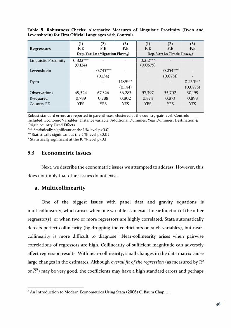
46
Table 5. Robustness Checks: Alternative Measures of Linguistic Proximity (Dyen and Levenshtein) for First Official Languages with Controls
(1) (2) (3) (1) (2) (3) Regressors F.E F.E F.E F.E F.E F.E
Dep. Var: Ln (Migration Flowsij) Dep. Var: Ln (Trade Flowsij)
Linguistic Proximity 0.822*** - - 0.212*** - - (0.124) (0.0675)
Levenshtein - -0.745*** - - -0.254*** -
(0.134) (0.0751) -
Dyen - - 1.189*** - - 0.430***
(0.144) (0.0775)
Observations 69,524 67,326 36,283 57,397 55,702 30,199
R-squared 0.789 0.788 0.802 0.874 0.873 0.898
Country FE YES YES YES YES YES YES
Robust standard errors are reported in parentheses, clustered at the country-pair level. Controls included: Economic Variables, Distance variable, Additional Dummies, Year Dummies, Destination & Origin country Fixed Effects. *** Statistically significant at the 1 % level p<0.01 ** Statistically significant at the 5 % level p<0.05 * Statistically significant at the 10 % level p<0.1
5.3 Econometric Issues
Next, we describe the econometric issues we attempted to address. However, this
does not imply that other issues do not exist.
a. Multicollinearity
One of the biggest issues with panel data and gravity equations is
multicollinearity, which arises when one variable is an exact linear function of the other
regressor(s), or when two or more regressors are highly correlated. Stata automatically
detects perfect collinearity (by dropping the coefficients on such variables), but near-
collinearity is more difficult to diagnose 8 .Near-collinearity arises when pairwise
correlations of regressors are high. Collinearity of sufficient magnitude can adversely
affect regression results. With near-collinearity, small changes in the data matrix cause
large changes in the estimates. Although overall fit of the regression (as measured by R2
or 𝑅2̅̅̅̅ ) may be very good, the coefficients may have a high standard errors and perhaps
8 An Introduction to Modern Econometrics Using Stata (2006) C. Baum Chap. 4.

47
even incorrect signs or implausibly high magnitudes. Another possible source of perfect
multicollinearity arises when using multiple binary or dummy variables as regressors,
known as the dummy variable trap. Generally, we avoid the multicollinearity problem
by excluding one of the binary variables as a standard practice. To test for
multicollinearity, we use the “Variance Inflation Factor (VIF)” defined as:
𝑉𝐼𝐹 = 1
(1 − 𝑅2)
VIF measures the degree to which variance has been inflated because one of the
regressor is not statistically independent. Also, 1 − 𝑅2 = 𝑡𝑜𝑙𝑒𝑟𝑎𝑛𝑐𝑒 𝑜𝑟 1/𝑉𝐼𝐹 is the
percentage of variance in the independent variable that is not accounted for by other
variables. VIF can be tested after fitting a regression model. As a rule of thumb, if the
mean VIF is greater than unity or if the largest VIF is greater than 10 then there is
evidence of collinearity. Table 6 below provides VIF values, maximum VIF is less than 2
collectively for both the migration and trade models that shows there is no perfect
correlation. However, mean VIF for both (migration flows and trade flows) is greater
than 1.00, which indicates that there might be some degree of correlation between
independent variables.
Table 6. Multicollinearity Diagnostic: The VIF Method
Ln (Migration Flowsij) Ln (Trade Flowsij) Variables VIF 1/VIF VIF 1/VIF
Linguistic Proximity Index
1.09 0.921344 1.05 0.953790
Ln GDP pCap _Dest_t-1 1.29 0.776016 1.45 0.691135 Ln GDP pCap _Orig_t-1 1.67 0.597229 1.49 0.670328 Ln Distance in km 1.12 0.895169 1.10 0.909665 Ln GDP_Dest_t-1 1.20 0.833396 1.23 0.815320 Ln GDP_Orig_t-1 1.60 0.623118 1.50 0.665550
Mean VIF 3.22 1.97

48
b. Heteroscedasticity and Serial Correlation
Serial correlation (or autocorrelation) occurs when one observation’s error term
is correlated with another observation’s error term. As error terms consists of time-
varying factors that affect the dependent variable but are not included as regressors,
some of these omitted factors may be autocorrelated and cause the standard errors of
the coefficients to be smaller and R2 to be larger than they would otherwise be. Because
our gravity model uses panel data on consecutive years for country pairs and with lagged
observation on some of the variables, autocorrelation is highly likely.
Heteroscedasticity states that the variance of the regression error terms
conditional on the regressors is not constant (the opposite as in the case of
homoscedasticity). To control for both heteroscedasticity and correlation over time, all
our estimates are based on robust standard errors. We have used the vce, (cluster id)
command in our regression estimations to yield standard errors that are robust to
heteroscedasticity and autocorrelation (using country-pair as id). This is a widely-used
command by researchers.
vce(robust-) uses the robust or sandwich estimator of variance. This estimator is
robust to some types of misspecification so long as the observations are
independent.
vce(cluster-) specifies that the standard errors allow for intragroup correlation,
relaxing the usual requirement that the observations be independent.
Observations are independent across groups (clusters) but not necessarily within
groups.
c. Endogeneity
The problem of endogeneity occurs when an explanatory variable is correlated
with the error term. As highlighted in the section above, we cannot completely
overcome this problem. However, it is partly addressed by using country-specific fixed
effects for both destination and source countries. Nevertheless, the complete absence of
omitted variable bias is not guaranteed.

49
d. Year-Fixed Effects and Country-Fixed Effects
It is important to include year-fixed effects in panel data regressions to control
for economic shocks such as booms and recessions that are common to all countries,
but that vary over time. Controlling for source-country, destination-country, and time-
fixed effects was done through dummy variables that assume the value 1 if a given
source/destination or year appears in the data in a particular observation, and 0
otherwise. By using these fixed effects, we find that our model has higher explanatory
power as compared to the conventional OLS model without fixed effects.
e. Other Econometric Concerns
We have tried to achieve the best possible unbiased coefficients in our regressions.
Still, some issue may remain. We attempted to control for some of these pitfalls through
robustness checks and by adding additional variables. The results in our robustness
checks are largely consistent with our main findings in the original empirical models,
though less so when it comes to the robustness of the variables GDP and GDP per capita
due to variation in their results.
There is also the possibility that using linguistic proximity as the only proxy for
culture may bias the results. There are other factors beyond language that reflect cultural
closeness, such as genetic distance, common traditions, and ethnicity, which we did not
take into account. Finally, we cannot rule out the importance of trade liberties and
preferential trade policies in enhancing business ties.
50
6. Comparative Analysis
An important objective of our research was to conduct a comparative analysis of
our augmented gravity models to estimate the impact of language on trade and
migration. To keep the comparison simple and straightforward, we used the same set of
variables in both the trade and migration models. The OLS regression with year- and
country-fixed effects and robust standard errors is the preferred method to accurately
predict our covariates. The gravity model appears to have been successful in explaining
most of the reasons why bilateral trade and migration varies across the full sample of
observations. Overall, we find that countries that are economically larger and relatively
closer in geographic distance are more engaged in bilateral trade and attract more
immigrants towards them. In addition, the Linguistic Proximity Index is found to be
highly significant in all specifications and behaves as expected with the gravity variables.
Our estimates are not only statistically significant but are also in line with the economic
literature. Taken together, gravity variables and cultural variables do a decent job at
explaining the causal relationship for both international migration and bilateral trade.
Using the same set of countries and similar econometric methods, and holding
other variables constant, we find that linguistic distance is highly significant in
determining trade flows and migration patterns between source/exporting and
destination/importing countries. As shown in the results section, the Linguistic
Proximity Index is positive and significant in all specifications (i.e. OLS and FE
regressions) in both models. However, the coefficient on linguistic proximity is much
larger for migration. This may imply that language is relatively more important in
migration decisions than it is in trade.
In terms of other independent variables, GDP, and GDP per capita in the
destination country was found to be statistically significant in both the trade and
migration models, but with opposing signs. In particular, GDP per capita had a negative
coefficient, while GDP had a positive coefficient for destination, in both models. While
this result may not be in line with economic theory, both GDP variables do behave

51
similarly in both models. For its part, geographic distance has almost the same impact
on both trade and migration models. Our results validate the economic theory that
countries that are relatively closer in geographical distance tend to attract more
immigrants and favor bilateral trade. Numerically, a 10% decrease in the physical
distance between the capital cities of two countries is associated with an increase in
aggregate trade volumes of almost 10% and an increase in migration flows of almost 11%.
We also find that linguistic distance and geographical distance have almost the same
impact on migration. For a potential migrant, language and distance are equally
important factors to consider in migration decisions.
We also use a statistical tool, fitting a seemingly unrelated regression SURE
model (Zellner, 1962) in its most basic form, to test whether our econometric equations
are related through the correlation in their error terms. This model takes into account
the fact that subtle interactions may be present between individual statistical
relationships when each of these relationships is being used to model some aspect of
behavior. The Stata output, is tabulated in Table 7 below:
Table 7. Seemingly Unrelated Regression (SURE)-Migration and Trade Equations
Variables SUREG (Migration) SUREG (Trade)
Linguistic Proximity Index 1.098*** 0.352***
(0.0280) (0.0232)
Ln GDP pCap _Dest_t-1 -2.334*** -2.248***
(0.177) (0.147)
Ln GDP pCap _Orig_t-1 -0.177*** 1.000***
(0.0610) (0.0507)
Ln Distance in km -1.076*** -0.951***
(0.00986) (0.00820)
Ln GDP_Dest_t-1 2.618*** 2.668***
(0.186) (0.155)
Ln GDP_Orig_t-1 -0.138** -0.599***
(0.0639) (0.0531)
Observations 69,524 69,524
R-squared 0.779 0.863
Country F.E YES YES

52
Correlation matrix of residuals:
Ln Migration Flowsijt Ln Trade Flowsijt
Ln Migration Flowsijt 1.0000
Ln Trade Flowsijt 0.2476 1.0000
Breusch-Pagan test of independence:
Chi2 (1)= 4260.892, Pr. = 0.0000
The summary output indicates that each equation explains almost all the
variation in the observation on migration and trade flows. The correlation matrix
displays the estimated VCE of residuals and test for independence of the residual vectors
(error terms). Sizeable correlations, all positive appears, and the Breusch-Pagan test
rejects its null of independence of these residual series at 1% level. We can also notice
that regression coefficients, standard errors, and R2 change their values with SURE
indicating eq. (1) and (2) from migration and trade models are related through residuals.
However, this does not change our interpretations on the original econometric models
under study.

53
7. Conclusions
In this thesis, we have tried to investigate the role of cultural differences on
migration and trade patterns using a refined indicator, the Language Proximity Index. A
gravity model approach is adopted for this purpose to capture and segregate economic
characteristics, geographical distribution, and cultural barriers for migration and trade.
Previous empirical research into the determinants of migration and trade had rarely
gone beyond using simple dummy for sharing a common language. In our research, we
instead adopt a sophisticated and more accurate measure of linguistic proximity.
Furthermore, few studies in the existing literature consider trade and migration patterns
in a parallel fashion as we have done. In fact, trade and migration determinants have
been studied through gravity equations either separately or with one as an explanatory
variable for the other. Instead, we believe there are many dynamics that are actually
common in both migration and trade patterns. Under our joint approach, we are able to
conduct a comparative analysis for migration and trade models to gain a better
understanding on our coefficients of interest. In this way, we have attempted to
contribute something new to the existing literature on the subject.
To address our research question, we use a panel dataset on migration flows and
trade flows from 223 source countries to 30 OECD destination countries around the
world, for the period 1980-2006. We initially employed conventional OLS on the full
sample of countries, then extended the analysis using fixed effect regressions, and finally
we check the robustness of our findings with the Poisson fixed effect method. Starting
with simple gravity variables, we take the analysis a step further by including additional
controls through dummies. For the most part, the results remain consistent across all
specifications with little variation. Based on our empirical model(s), we conclude that:
Language proximity is highly significant across all model specifications and all
the econometric approaches used. We find that migration rates and trade
volumes are higher between countries whose first official languages are closer.
The results are robust to the use of two alternate measures of linguistic distance

54
(i.e. Levenshtein distance and Dyen linguistic proximity). Furthermore, linguistic
distance poses a relatively greater barrier for migration than for bilateral trade.
Traditional economic push and pull factors, like GDP per capita and real GDP,
interact differently for migration and trade. This contradicts economic theory
that levels of GDP should positively affect bilateral trade and migration flows
both for sending and receiving countries. However, these results do not sharply
contrast previous literature. We can say that linguistic proximity does a better
job of explaining the determinants of the direction of migration flows and trade
patterns due to consistency of their results, compared to differentials in economic
variables.
Geographical distance has a statistically and economically significant impact on
trade and migration flows in all sets of models. Countries that are geographically
farther apart trade less, and countries that are geographically closed have greater
migration inflows at a particular destination. In addition, linguistic distance and
physical distance are found to have almost same impact on migration and on
trade. Although the magnitude of the physical distance effect and linguistic
distance effect on migration and on trade has been different through various
econometric methods, their sign and significance endure the hardship of
scientific scrutiny.
The extension of models using robustness dummies finds that countries
belonging to the same regional trade associations trade more. Furthermore, a
shared colonial history encourages trade and is also conducive to an increased
influx of immigrants. Meanwhile, a dummy for whether the countries are
neighbors has a significantly positive impact for trade, but insignificant for
migration. Finally, we find that membership in the GATT/WTO is associated with
a surprisingly insignificant impact on trade. This also challenges the general
perception that multilateral trade organizations like the WTO promote trade.
Although we control for observations with value zero, endogeneity, and
heteroscedasticity, there remains a risk of measurement error or bias in our results.
However, overall our empirical strategy based on the gravity model works well in
explaining most of the factors contributing to variations in trade flows and migration

55
patterns. Furthermore, language similarity has a substantial effect on trade and
migration above and beyond gravitational effects. This finding opens the door to
potential future discussions on the topic. As patterns of trade and migration are
influenced by an interplay of several other determinants, choosing an instrumental
variable may be an interesting approach to infer a causal relationship within migration
and trade. Cultural barriers (as we find) dampen migration flows and bilateral trade, but
immigrants can counter the effects of this cultural distance on trade and vice versa, as
product diversity requires ethnic diversity. We have studied trade flows and migration
patterns exclusively to OECD destinations, which are developed countries. However,
there is reason to believe that the mechanism driving migration and trade between
developed countries will be different than those driving migration and trade between
developing and developed countries.

56
Bibliography
Anderson, J. E. (1979). A Theoretical Foundation for the Gravity Equation. The American Economic
Review, 69(1), 106-116 .
Anderson, J. E. (2011). The Gravity Model. Annual Review of Economics, 3(1), 133-160.
Barry R.Chiswick, P. W. (2015). Handbokk of the Economics of International Migration. Elsevier.
Baum, C. F. (2006). An Introduction to Modern Econometrics Using Stata. Texas: StataCorp LP.
Belot , M., & Ederveen , S. (2012). Cultural Barriers in Migration Between OECD Countries. Journal
of Population Economics.
Bergstrand, J. H. (1985). The Gravity Equation in International Trade: Some Microeconomic
Foundations and Empirical Evidence. The Review of Economics and Statistics, 67(3), 474-
481.
Brakman, P. A. (2010). The Gravity Model in International Trade. Cambridge: Cambridge University
Press.
CEPII Gravity Database. (2018). Hentet fra
http://www.cepii.fr/cepii/en/bdd_modele/presentation.asp?id=8
Christian Thiemann. (2010). The Structure of Borders in a Small World. PLoS ONE, 5(11).
Cohen, K. K. (2010). Determinants of International Migration Flows to and from Industrialized
Countries: A Panel Data Approach Beyond Gravity. The International Migration Review,
44(4), 899-932.
David Karemera, V. I. (2010). A gravity model analysis of international migration to North America.
Applied Economics , Volume 32, 2000 (13), 1745-1755.
De, P. (2013). Assessing Barriers to Trade in Services in India: An Empirical Investigation. Journal of
Economic Integration, 28(1), 108-143.
Ederveen, M. B. (2012). Cultural barriers in migration between OECD countries. Journal of
Population Economics, 25(3), 1077-1105.
Egger, P. (2000). A note on the proper econometric specification of the gravity equation. Economic
Letters, 66(1), 25-31.
Feenstra, R. C. (2016). Advanced International Trade: Theory and Evidence. New Jersey: Princeton
University Press.
Filippo Simini, M. C.-L. (2012). A universal model for mobility and migration patterns. Nature, 484,
ss. 96-100.

57
Friberg, J. H. (2012). 13. The stages of migration from going abroad to settling down : Post
Accession Polish migrant workers in Norway. Journal of Ethnic and Migration Studies,
38(10), 1589-1605.
Gabriel & Toubal, 2. (2010). Cultural Proximity and Trade. European Economic Review, 54(2), 279-
293.
Gautier Krings, F. C. (2009). Urban gravity: a model for inter-city telecommunication flows. Journal
of Statistical Mechanics: Theory and Experiment, 2009.
Gidwani, V., & Sivaranakrishan, k. (2004). Circular Migration and the Spaces of Cultural Assertion.
Wiley Online Library.
Giuliano, A. A. (2015). Culture and Institutions. Journal of Economic Literature, 53(4), 898-944.
Gokmenn, G. (2017). Clash of Civilization and the Impact of Cultural Differences on Trade. Journal
of Development Economics.
Gourdon, J. (2009). Journal of Economic Integration, 24(1).
Head, K. a. (2015). Gravity Equations: Toolkit, Cookbook, Workhorse. 4, 131-195. (H. o. Economics.,
Red., & K. R. Elhanan Helpman, Kompilator) Elsevier. Hentet fra
https://sites.google.com/site/hiegravity/
Head, K. M. (2010). The erosion of colonial trade linkages after independence. Journal of
International Economics, 81(1), 1-14.
International Migration Report. (2017). The United Nations, Department of Economic and Social
Affairs Population Division . New York: The United Nations.
Isaac, J. (1947). Economics of Migration. (D. K. Mannheim, Red.) London: hunt, Barnard and Co.
Ltd.
J.Felbermayrt, G., & Toubal, F. (2007). Cultural Proximity and Trade.
J.Lewera, J., & Bergb, H. d. (2008). A gravity model of immigration. Economic Letters, 99(1), 164-
167.
Jacques Melitz, F. T. (2014). Native language, spoken language, translation and trade. Journal of
International Economics, 93(2), 351 to 363.
JAIN, S. M. (2015). Determinants of OFDI: An Empirical Analysis of OECD Source Countries using
Gravity Model. Indian Economic Review, New Series, 50(2), 243-271 .
James E. Anderson, E. v. (2003). Gravity with Gravitas: A Solution to the Border Puzzle. American
Economic Review, 93(1), 170-192.
Kingsley, G. (1946). The P1 P2/D Hypothesis: On the Intercity Movement of Persons. American
Sociological Review, , 11(6), 677-686.

58
Klay, S. (2011). Explaining the stages of migration within a life course framework. European
Sociological Review, 27(4), 469-486.
Kónya, I. (2006). Modeling Cultural Barriers in International Trade. Review of International
Economics, 14(3), 494-507.
Ku, H., & Zussman, A. (2010). Lingua Franca: The Role of English in International Trade. Journal of
Economic Behavior and Organization.
Lassmann, P. E. (2011). The Language Effect in International Trade: A Meta-Analysis. CESifo
Working Paper Series 3682, CESifo Group Munich.
Liu, C. W. (2010). Determinants of Bilateral Trade Flows in OECD Countries: Evidence from
Gravity Panel Data Models. The World Economy, 33(7), 894-915.
Lohmann, J. (2011). Do Language Barriers affect Trade. Economic Letters.
MarcBarthélemy. (2011). Spatial Networks. Physics Reports, 499(1-3), 1-101.
Mauro Lanati, A. V. (2018). Cultural Change and the Migration Choice. IZA Discussion Paper No.
11415.
Mayda, A. M. (2010). International Migration: A Panel Data Analysis of the Determinants of
Bilateral Flows. Journal of Population Economics, 23(4), 1249-1274.
Melitz, J., & Toubal, F. (2014). Native Language, Spoken Language, Translation and Trade. Journal
of International Economics.
Migration and Migrants: A Global Overview , World Migration Report (2018). Geneva: International
Organization for Migration.
Millimet, D. J. (2008). Is Gravity Linear? Journal of Applied Econometrics, 23(2), 137-172.
Nicita, A., & Tumurchudur-Klok, B. (u.d.). Geneva: UNCTAD.
Organisation for Economic Co-operation and Development. (2017). Hentet fra National Accounts -
OECD: http://www.oecd.org/sdd/na/
Pablo Kaluza, A. K. (2010). The complex network of global cargo ship movements. J. R. Soc.
Interface, 7(48), 1093-1103.
Peter H.Egger, A. (2012). The language effect in international trade: A meta-analysis. Economics
Letters, 116(2), 221-224.
Peter Egger. (2000). A note on the proper econometric specification of the gravity equation.
Economics Letters, 66(1), 25-31.
Pytliková, A. A. (2015). The Role of Language in Shaping International Migration. The Economic
Journal, 125(586), F49-F81 (Feature Issue).
Pöyhönen, P. (1963). A Tentative Model for the Volume of Trade between Countries. (w. JSTOR,
Red.) Weltwirtschaftliches Archiv, 90(1963), 93-100.

59
ROSE, A. K. (2004). Do We Really Know That the WTO Increases Trade? The American Economic
Review, 94(1), 98-114.
The World Bank. (2017). Hentet fra World Bank National Accounts Data :
https://data.worldbank.org/
Thomlinson, R. (1961). A Model for Migration Analysis. Journal of the American Statistical
Association, 56(295), 675-686.
Tiiu Paas, E. T. (2008). Gravity Equation Analysis in the Context of International Trade: Model
Specification Implications in the Case of the European Union. Eastern European Economics,
46(5), 92-113.
UN-DESA. (2015). World Population Prospects. Hentet fra The United Nations Department of
Economic and Social Affairs:
https://esa.un.org/unpd/wpp/publications/files/key_findings_wpp_2015.pdf
UNDP. (2009). United Nations Development Program. Hentet fra
http://www.undp.org/content/undp/en/home/librarypage/corporate/undp_in_action_200
9.html
VANDERKAMP, J. (1977). THE GRAVITY MODEL AND MIGRATION BEHAVIOUR: AN
ECONOMIC INTERPRETATION. Journal of Economic Studies, 4(2), 89-102.
VK Srivastava, D. G. (1987). Seemingly Unrelated Regression Equations: Estimation and Inference.
New York: Marcel Dekker Inc.
Watson, J. H. (2015). Introduction to Econometrics. London: Pearson.
Weber, V. G. (Red.). (2016). The Palgrave Handbook of Economics and Language. London: Palgrave
Macmillan.
White, R. (2016). Cultural Differences and Economic Globalization: Effects on Trade, Foreign Direct
Investment, and Migration. Oxon and New York: Routledge.
Wincoop, J. E. (2003). Gravity with Gravitas: A Solution to the Border Puzzle. The American
Economic Review, 93(1), 170-192.
Woo-Sung Jung, F. W. (2008). Gravity Model in the Korean Highway. Europhysics Letters
Association, 81(4).
Zellner, A. (1962). Journal of the American Statistical Association.
Zimmermann, A. F. (Red.). (2013). International Handbook on the Economics of Migration.
Cheltenham , UK: Edward Elgar.
Zimmermann, K. F., & Bauer, T. (Red.). (2002). The Economics of Migration (Vol. 1). Cheltenham:
Edward lgar Publishing Inc.
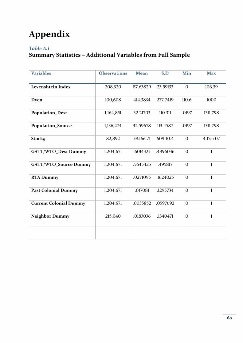
60
Appendix
Table A.1
Summary Statistics – Additional Variables from Full Sample
Variables Observations Mean S.D Min Max
Levenshtein Index 208,320 87.63829 23.59133 0 106.39
Dyen 100,608 414.3834 277.7419 110.6 1000
Population_Dest 1,164,851 32.21703 110.311 .0197 1311.798
Population_Source 1,136,274 32.59678 113.4587 .0197 1311.798
Stockij 82,892 38266.71 609110.4 0 4.17e+07
GATT/WTO_Dest Dummy 1,204,671 .6014323 .4896036 0 1
GATT/WTO_Source Dummy 1,204,671 .5645425 .495817 0 1
RTA Dummy 1,204,671 .0271095 .1624025 0 1
Past Colonial Dummy 1,204,671 .017081 .1295734 0 1
Current Colonial Dummy 1,204,671 .0035852 .0597692 0 1
Neighbor Dummy 215,040 .0183036 .1340471 0 1

61
Table A.2
List of Variables and Definition – Full Sample
Variable Definition
Year Observation year
ID Pair of country ID (Destination + Source)
Destination Name of destination country j
Source Name of source country i
Migration Flowij Immigration inflow from country i to j
Trade Flowij Trade volume, Export or import
Linguistic Proximity Index Measure of language closeness or distance - official language
Levenshtein Max P distance between official languages
Dyen Dyen linguistic proximity between first official languages
Distance Capitals Distance between capital cities in kilometers
GDP pCap_Destination GDP per Capita in US $ in destination
GDP pCap_Source GDP per Capita in US $ in source
GDP_Destination GDP in US $ in destination
GDP_Source GDP in US $ in source
Stockij Foreign population from country i residing in j
GATT/WTO_ Dest Dummy variable = 1 if destination is GATT/WTO member
GATT/WTO_ Source Dummy variable = 1 if source is GATT/WTO member
RTA Dummy variable = 1 if Regional Trade Agreement in force
Colonial History Dummy Variable = 1 for pair ever in colonial relationship
Colonial Current Dummy Variable = 1 for pair currently in colonial relationship
Neighbor Dummy Variable= 1 for neighbor country, destination and source share a common border

62
Table A.3
List of OECD Destination Countries
Name of the countries
1. Australia 16. Korea
2. Austria 17. Luxembourg
3. Belgium 18. Mexico
4. Canada 19. Netherlands
5. Czech Republic 20. New Zealand
6. Denmark 21. Norway
7. Finland 22. Poland
8. France 23. Portugal
9. Germany 24. Slovak republic
10. Greece 25. Spain
11. Hungary 26. Sweden
12. Iceland 27. Switzerland
13. Ireland 28. Turkey
14. Italy 29. United Kingdom
15. Japan 30. United States
Source Countries All world countries, total 223 in number.

63
Table A.4
Definitions and Technical Notes Migration Flow: Migration flow is the inflow of immigrants to a destination from a given origin in
a given year. The definition usually covers immigrants coming for a period of half year or longer.
Flow refers to the number of migrants entering or leaving a country during a given period.
International Migrant: any person who changes his or her country of usual residence.
Foreign Population Stock: It is the total number of foreigners or international migrants from a
given source country living in a particular destination in a given year.
Citizenship and Country of Birth: The main criteria used for categorizing migrant stock and flows
are country of birth and citizenship. Citizenship indicates the particular legal bond between an
individual and his/her country, acquired by birth or naturalization, whether by declaration, choice,
marriage, or other. Country of Birth refers to the country of residence of the mother at the time of
the birth or, in default, the country in which the birth took place.
Trade Flow: Total Trade values either imports or exports for all country-pairs. One country’s exports
are other country’s import, in a way flow from exporting country to importing country.
Destination and Source countries: In migration context, destination is the country that receives
immigrants from various source countries which are sending these immigrants. In respect to trading
partners, exporting country is the source country, and destination is the importing country.
Linguistic Proximity: Language similarity or closeness. The Linguistic Proximity Index ranges from
0 to 1, depending on how many levels of linguistic family tree the languages of both countries share.
Bilateral Trade: It is the exchange of goods between two countries.
Gravity Model: Gravity model is a model used to estimate the amount of interaction between two
entities. It is based on Newton’s universal law of gravitation.
GDP and GDP per Capita: Gross domestic product defines size of a country and GDP per capita
(GDP divided by population) captures development effects. So together they describe how strong
and rich an economy is.
Multicollinearity: Generally, occurs when there is high correlation between two or more predictor
variables. In a way one predictor can be used to predict the other.
Endogeneity: This problem occurs when an explanatory variable is correlated with the error term.
Endogeneity arises as a result of measurement error, serial correlation, simultaneous causality,
selection bias and omitted variables.
Autocorrelation: Serial correlation or autocorrelation occurs when one observation’s error term is
correlated with another observation’s error term. In a way, error terms in a time series or cross section
data transfers from one period to another. Serial correlation is problematic, as it causes standard
errors of the coefficients to be smaller and R-squared higher than otherwise.