Embed Size (px)
Citation preview
THE UNIVERSITY OF ADELAIDE
Landscape scale measurement and monitoring of
biodiversity in the Australian rangelands
Thesis presented for the degree of
Doctorate of Philosophy
Kenneth Clarke
B. Env. Mgt. (Hons), University of Adelaide
November 2008
Faculty of Sciences, Discipline of Soil and Land Systems

Abstract
i
Abstract
It is becoming increasingly important to monitor biodiversity in the extensive Australian
rangelands; currently however, there is no method capable of achieving this goal. There
are two potential sources of relevant data that cover the Australian rangelands, and from
which measures of biodiversity might be extracted: traditional field-based methods such as
quadrat surveys have collected flora and fauna species data throughout the rangelands, but
at fine scale; satellite remote sensing collects biologically relevant, spatially
comprehensive data. The goal of this thesis was to provide the spatially comprehensive
measure of biodiversity required for informed management of the Australian rangelands.
The study specifically focused on the Stony Plains in the South Australian rangelands. To
that end the thesis aimed to develop indices capable of measuring and/or monitoring
biodiversity from vegetation quadrat survey data and remotely sensed data.
The term biodiversity is so all-encompassing that direct measurement is not possible;
therefore it is necessary to measure surrogates instead. Total perennial vegetation species
richness (γ-diversity) is a sound surrogate of biodiversity: the category of species is well
defined, species richness is measurable, and there is evidence that vegetation species
richness co-varies with the species richness of other taxonomic groups in relation to the
same environmental variables.
At least two broad scale conventional vegetation surveys are conducted in the study region;
the Biological Survey of South Australia; and the South Australian Pastoral Lease
Assessment. Prior to the extraction of biodiversity data the quality of the BSSA, the best
biodiversity survey, was evaluated. Analysis revealed that false-negative errors were
common, and that even highly detectable vegetation species had detection probabilities
significantly less than one. Without some form of correction for detectability, the species-
diversity recorded by either vegetation survey must be treated with caution.
Informed by the identification of false-negative errors, a method was developed to extract
γ-diversity of woody perennials from the survey data, and to remove the influence of
sampling effort. Data were aggregated by biogeographic region, rarefaction was used to
remove most of the influence of sampling effort, and additional correction removed the
residual influence of sampling effort. Finally, additive partitioning of species diversity
Abstract
ii
allowed extraction of indices of α-, β- and γ-diversity free from the influence of sampling
effort. However, this woody perennial vegetation γ-diversity did not address the need for a
spatially extensive, fine scale measure of biodiversity at the extent of the study region.
The aggregation of point data to large regions, a necessary part of this index, produces
spatially coarse results.
To formulate and test remotely sensed surrogates of biodiversity, it is necessary to
understand the determinants of and pressures on biodiversity in the Australian rangelands.
The most compelling explanation for the distribution of biodiversity at the extensive scales
of the Australian rangelands is the Productivity Theory, which reasons that the greater the
amount and duration of primary productivity the greater the capacity to generate and
support high biodiversity. The most significant pressure on biodiversity in the study area
is grazing-induced degradation, or overgrazing.
Two potential spatially comprehensive surrogates of pressure on biodiversity were
identified. The first surrogate was based on the differential effect of overgrazing on water-
energy balance and net primary productivity: water-energy balance is a function of climatic
variables, and therefore a measure of potential or expected primary productivity; net
primary productivity is reduced by high grazing pressure. The second surrogate was based
on the effect of grazing-induced degradation on the temporal variability of net primary
productivity: overgrazing reduces mean net primary productivity and rainfall use
efficiency, and increases variation in net primary productivity and rainfall use efficiency.
The two surrogates of biodiversity stress were derived from the best available remotely
sensed and climate data for the study area: actual evapotranspiration recorded by climate
stations was considered an index of water-energy balance; net primary productivity was
measured from NOAA AVHRR integrated NDVI; rainfall use efficiency (biomass per unit
rainfall) was calculated from rainfall data collected at climate stations and the net primary
productivity measure. Finally, the surrogates were evaluated against the index of woody
perennial α-, β- and γ-diversity, on the assumption that prolonged biodiversity stress would
reduce vegetation species diversity.
No link was found between Surrogate 1 and woody perennial α-, β- or γ-diversity. The
relationship of Surrogate 2 to woody perennial diversity was more complex. Only some of
Abstract
iii
the results supported the hypothesis that overgrazing decreases α-diversity and average
NPP and RUE. Importantly, none of the results supported the most important part of the
hypothesis that the proposed indices of biodiversity pressure would co-vary with woody
perennial γ-diversity. Thus, the analysis did not reveal a convincing link between either
surrogate and vegetation species diversity. However, the analysis was hampered to a large
degree by the climate data, which is interpolated from a very sparse network of climate
stations.
This thesis has contributed significantly to the measurement and monitoring of biodiversity
in the Australian rangelands. The identification of false-negative errors as a cause for
concern will allow future analyses of the vegetation survey data to adopt methods to
counteract these errors, and hence extract more robust information. The method for
extracting sampling effort corrected indices of α-, β- and γ-diversity allow for the
examination and comparison of species diversity across regions, regardless of differences
in sampling effort. These indices are not limited to rangelands, and can be extracted from
any vegetation quadrat survey data obtained within a prescribed methodology. Therefore,
these tools contribute to global biodiversity measurement and monitoring. Finally, the
remotely sensed surrogates of biodiversity are theoretically sound and applicable in any
rangeland where over-grazing is a significant source of degradation. However, because the
evaluation of these surrogates in this thesis was hampered by available data, further testing
is necessary.

Acknowledgements
iv
Acknowledgements
I would like to say that my parents, David and Denece Clarke, are to blame for this thesis.
They are ultimately, through my creation, responsible for the work herein. However, there
are more proximate reasons to point the finger at Mum and Dad: it was they who instilled
in me an appreciation of the wonder of the natural world; who encouraged my questions;
who discouraged assumptions and mental laziness in general; who showed me that there is
no shame in testing with evidence and admitting error; who taught me that hard work is
important, but needs to be balanced with play; and most importantly, in each of these they
led by example. My most heartfelt thanks to Mum and Dad.
I would also like to thank my fiancée, Claire Davill, for supporting me throughout this
endeavour, for reading drafts, offering advice, cooking muffins and just generally being
there for me. You are much appreciated.
This research was conducted under the supervision of Associate Professor Megan Lewis
and Dr Bertram Ostendorf of the University of Adelaide, and David Hart, South Australian
Department of Environment and Heritage. I’d like to thank Megan for her amazingly
prompt responses, her intelligent dissections of my attempts at writing and her very
welcome ability to see both the small and big pictures. I’ve learned more about writing
under Megan’s tutelage than I did in three years of undergrad and five years of high
school. I’d like to thank Bertram for his conception of the rarefaction approach, advice on
drafts, and for organising an incredibly interesting conference in China. Sweet. Dave Hart
is thanked for agreeing at the 11th (possibly the 14
th or 15 hour) to be an external supervisor
(like a dermatologist?), for advice on some of my writing, and for being a kindred spirit.
I would like to thank the Desert Knowledge Cooperative Research Centre (DK CRC) for
their financial support, both scholarship and operating funds, without which this may not
have been possible. The student forums run by the DK CRC were also of great value in
providing networking opportunities, and for the specific workshops and presenters.
Special thanks to Alicia Boyle for making communication with the CRC not just easy, but
also pleasant. Additionally, I would like to thank the University of Adelaide for the
Divisional Scholarship which provided the bulk of my income and thus allowed me to eat

Acknowledgements
v
and put a roof over my head, both of which were probably essential to the completion of
the PhD.
For the provision of the climate data at a reasonable price I owe thanks to Dr Greg
Kociuba, Queensland Climate Change Centre of Excellence.
I’d like to thank many of the post grads who make up the wonderful spatial information
group (SIG), and some ring-ins: Dave Summers, Greg Lyle, Anna Dutkiewicz, Sean
Mahoney, Dorothy Turner, Rowena Morris, Paul Bierman, Ramesh Raja Segaran, Ben
Conoley, Tonja Wright, Sjaan Davey, Adam Kilpatrick and Troy Willats. Special thanks
to those who joined me for morning tea, almost every day, who in addition to those already
mentioned included Dr’s Neville Crossman and Patrick O’Connor.
Almost there dear reader. I’d like to thank our various ladies at reception, Therese Dean,
Marie Norris, Susan Saunders and those who’s names I’ve forgotten (also, my apologies
for the forgetting). Also, thanks to Deb Miller, who’s not a receptionist but does dwell
near reception and is very helpful, good value and is quite appreciated.
For permission to reproduce her excellent photo of rain coming in over the Simpson
Desert, Australia, I owe thanks to Patricia Mc, and to Flikr for helping me to locate
Patricia’s photo.
Finally, to you dear reader: if you’re reading this you are one of the few people who will
ever read this acknowledgements section, and are to be commended for your persistence. I
hope you will find the rest of the thesis an engaging, or at least informative read. As the
ancient Assyrians used to say, “May your reading be swift and fruitful.”

Declaration
vi
Declaration
This work contains no material which has been accepted for the award of any other degree
or diploma in any university or other tertiary institution and, to the best of my knowledge
and belief, contains no material previously published or written by another person, except
where due reference has been made in the text.
I give consent to this copy of my thesis when deposited in the University Library, being
made available for loan and photocopying, subject to the provisions of the Copyright Act
1968.
The author acknowledges that copyright of published works contained within this thesis (as
listed below) resides with the copyright holder(s) of those works.
Signed: ___________________ Date: _______________
Kenneth David Clarke
Publications arising from this thesis
vii
Publications arising from this thesis
Refereed publications
Clarke, K.D., Lewis, M.M., and Ostendorf, B. ‘False negative errors in a survey of
persistent, highly-detectable vegetation species.’ Applied Vegetation Science (submitted).
Clarke, K.D., Lewis, M.M., and Ostendorf, B. ‘Additive partitioning of rarefaction curves:
removing the influence of sampling on species-diversity in vegetation surveys.’
Ecological Indicators (submitted).
Conference poster
Clarke, K.D., Lewis, M.M., and Ostendorf, B. (2006) Limitations of vegetation surveys:
characterising plant species richness. The 14th
Biennial Conference of the Australian
Rangeland Society: Renmark, South Australia.
Award
Best student paper at conference (2006) 14th Biennial Conference of the Australian
Rangeland Society: Renmark, South Australia.
Publications arising from this thesis
viii
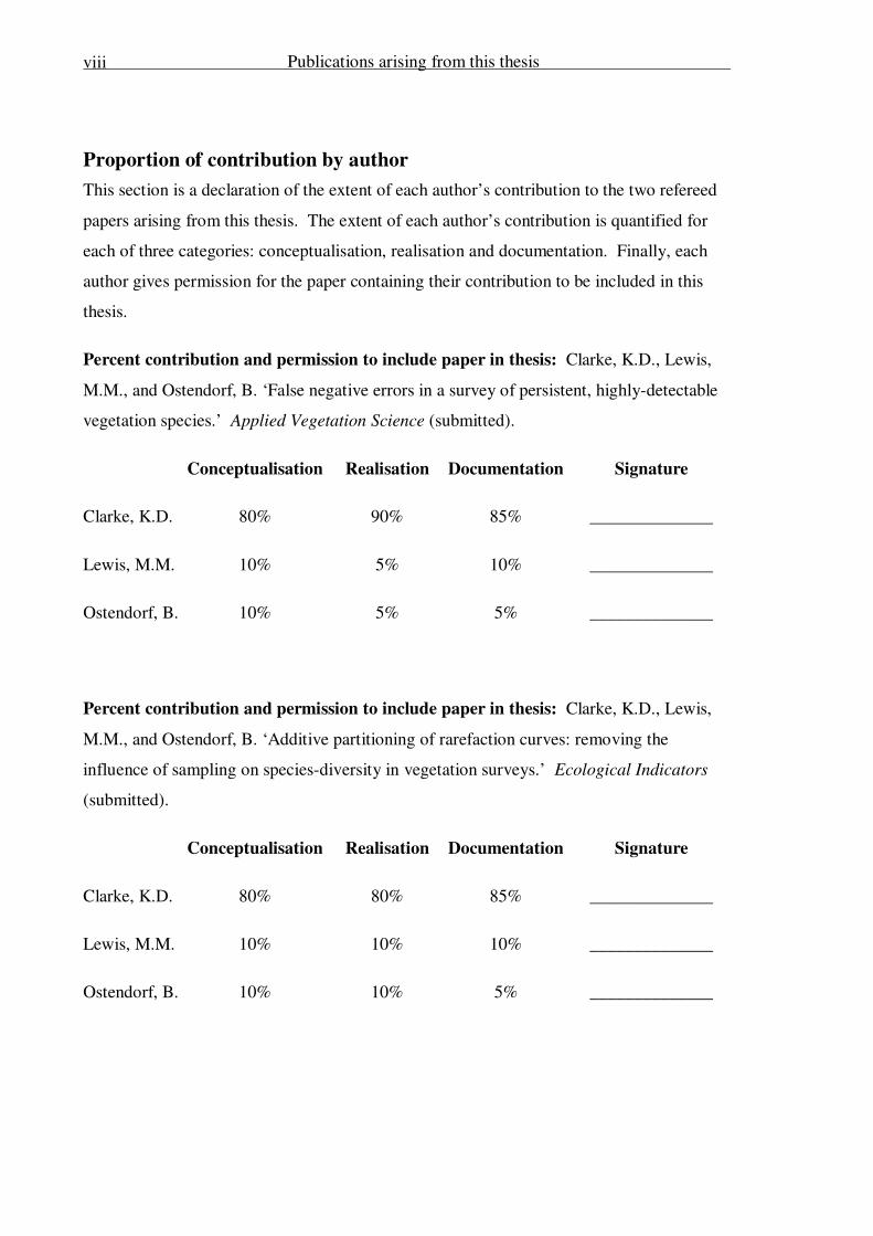
Proportion of contribution by author
This section is a declaration of the extent of each author’s contribution to the two refereed
papers arising from this thesis. The extent of each author’s contribution is quantified for
each of three categories: conceptualisation, realisation and documentation. Finally, each
author gives permission for the paper containing their contribution to be included in this
thesis.
Percent contribution and permission to include paper in thesis: Clarke, K.D., Lewis,
M.M., and Ostendorf, B. ‘False negative errors in a survey of persistent, highly-detectable
vegetation species.’ Applied Vegetation Science (submitted).
Conceptualisation Realisation Documentation Signature
Clarke, K.D. 80% 90% 85% ______________
Lewis, M.M. 10% 5% 10% ______________
Ostendorf, B. 10% 5% 5% ______________
Percent contribution and permission to include paper in thesis: Clarke, K.D., Lewis,
M.M., and Ostendorf, B. ‘Additive partitioning of rarefaction curves: removing the
influence of sampling on species-diversity in vegetation surveys.’ Ecological Indicators
(submitted).
Conceptualisation Realisation Documentation Signature
Clarke, K.D. 80% 80% 85% ______________
Lewis, M.M. 10% 10% 10% ______________
Ostendorf, B. 10% 10% 5% ______________
Table of contents
ix
Table of contents
Abstract ............................................................................................................................ i
Acknowledgements ......................................................................................................... iv
Declaration ..................................................................................................................... vi
Publications arising from this thesis ............................................................................. vii
Table of contents ............................................................................................................ ix
List of Figures ............................................................................................................... xiv
List of Tables ............................................................................................................... xvii
Chapter 1: Introduction .................................................................................................. 1
1.1 Motivation for the research ..................................................................................... 1
1.2 Thesis topic and structure ....................................................................................... 3
1.3 Study area .............................................................................................................. 4
1.3.1 Location and infrastructure ............................................................................. 4
1.3.2 Physical geography and climate ..................................................................... 5
1.3.3 Ecology and land use ..................................................................................... 8
1.3.4 Conservation objectives ............................................................................... 12
1.4 References ............................................................................................................ 17
Chapter 2: Literature review ........................................................................................ 18
2.1 Introduction .......................................................................................................... 18
2.1.1 Biodiversity phenomena: α-, β- and γ-diversity ............................................ 18
2.1.2 Scale in biodiversity studies ......................................................................... 18
2.1.3 Determinants of biodiversity ........................................................................ 20
Climate and productivity .............................................................................. 20
Topography .................................................................................................. 23
Topographic redistribution of rainfall ........................................................... 24
Area and heterogeneity ................................................................................. 25
Soil type ....................................................................................................... 27
The influence of environmental variability on speciation .............................. 28
Fire .............................................................................................................. 29
2.1.4 Pressures on biodiversity .............................................................................. 30
Grazing induced degradation ........................................................................ 30
Exotic species invasion ................................................................................ 33
2.2 Surrogates for monitoring biodiversity ................................................................. 34
Table of contents
x
2.2.1 Generalised dissimilarity modelling ..............................................................34
2.2.2 Vegetation community classification.............................................................35
2.2.3 Indicators of landscape condition: rainfall use efficiency (RUE) and net
primary productivity (NPP) ........................................................................................36
2.2.4 Measures of landscape heterogeneity ............................................................37
Spectral variation ..........................................................................................37
Landscape leakiness ......................................................................................39
2.2.5 Airborne gamma-ray spectrometry ................................................................40
2.3 Summary and potential biodiversity surrogates .....................................................42
2.3.1 Surrogate 1 ...................................................................................................42
2.3.2 Surrogate 2 ...................................................................................................43
References .......................................................................................................................44
Chapter 3: False-negative errors in a survey of persistent, highly-detectable
vegetation species ...........................................................................................................49
3.1 Introduction ..........................................................................................................49
3.2 Methodology .........................................................................................................50
3.2.1 Study Area ....................................................................................................50
3.2.2 Survey data ...................................................................................................52
3.2.3 False-negative analysis .................................................................................53
Biological Survey of South Australia ............................................................53
3.3 Results ..................................................................................................................54
3.3.1 Biological Survey of South Australia ............................................................54
Site 9599.......................................................................................................55
Site 11031 .....................................................................................................55
Site 10478 .....................................................................................................56
Site 10294 .....................................................................................................57
Detection Probability ....................................................................................57
3.4 Discussion .............................................................................................................58
3.4.1 Ramifications for similar vegetation surveys .................................................60
3.4.2 Wider implications........................................................................................61
3.5 Acknowledgements ...............................................................................................62
3.6 References ............................................................................................................63
Chapter 4: Additive partitioning of rarefaction curves: removing the influence of
sampling on species-diversity in vegetation surveys .....................................................64
Table of contents
xi
4.1 Introduction .......................................................................................................... 64
4.1.1 The influence of sample-grain and sampling effort ....................................... 66
4.1.2 Research aims .............................................................................................. 67
4.2 Methods ............................................................................................................... 68
4.2.1 Study area .................................................................................................... 68
4.2.2 Survey data .................................................................................................. 68
Consistency of sample-grain ........................................................................ 70
Units of aggregation and sampling effort ...................................................... 71
4.2.3 Rarefaction................................................................................................... 71
Additive partitioning of rarefaction curves ................................................... 72
Rarefaction as a control for differences in sampling effort ............................ 73
Removal of sampling effort-influence .......................................................... 74
4.3 Results ................................................................................................................. 75
4.3.1 Rarefied diversity ......................................................................................... 75
4.3.2 Common sampling effort rarefaction ............................................................ 77
4.3.3 Removal of sampling effort influence ........................................................... 79
4.4 Discussion ............................................................................................................ 79
4.5 Acknowledgements .............................................................................................. 82
4.6 References ............................................................................................................ 83
Chapter 5: Remotely sensed surrogates of biodiversity stress ..................................... 85
5.1 Introduction .......................................................................................................... 85
5.2 Methods ............................................................................................................... 86
5.2.1 Study area .................................................................................................... 86
5.2.2 Common components ................................................................................... 87
Net primary production (NPP)...................................................................... 87
Topographic index: valley bottom flatness (VBF) ........................................ 89
5.2.3 Surrogate 1 ................................................................................................... 90
Expected primary production (EPP) ............................................................. 90
Topographically scaled EPP (TEPP) ............................................................ 91
Calculation of Surrogate 1 ............................................................................ 91
5.2.4 Surrogate 2 ................................................................................................... 92
Rainfall ........................................................................................................ 92
Climatically distributed rainfall use efficiency (CRUE) ................................ 92
Table of contents
xii
Topographically redistributed rainfall use efficiency (TRUE) .......................93
Calculation of Surrogate 2 ............................................................................93
5.2.5 Evaluation method ........................................................................................93
5.3 Results ..................................................................................................................94
5.3.1 Common component: index of valley bottom flatness (VBF) ........................94
5.3.2 Surrogate 1 ...................................................................................................96
Total net primary production (TNPP) ............................................................96
Expected primary production (EPP) ..............................................................96
Topographically scaled EPP (TEPP) .............................................................98
Surrogate 1: final index .................................................................................99
Evaluation of Surrogate 1............................................................................ 101
5.3.3 Surrogate 2 ................................................................................................. 102
Average annual NPP (mean-NPP) ............................................................... 102
Variation in annual NPP (std-NPP) ............................................................. 103
Average annual climatically distributed RUE (mean-CRUE) ...................... 104
Variation in annual climatically distributed RUE (std-CRUE) ..................... 106
Average annual topographically scaled RUE (mean-TRUE) ....................... 106
Variation in annual topographically scaled RUE (std-TRUE) ...................... 107
Evaluation of Surrogate 2............................................................................ 109
5.4 Discussion ........................................................................................................... 111
5.4.1 Summary .................................................................................................... 115
5.5 References .......................................................................................................... 116
Chapter 6: Discussion and conclusions ....................................................................... 120
6.1 Introduction ........................................................................................................ 120
6.2 Summary of specific contributions to knowledge ................................................ 121
6.2.1 False-negative errors in a survey of vegetation species ................................ 121
6.2.2 Additive partitioning of rarefaction curves species diversity surrogate ........ 122
6.2.3 Remotely sensed biodiversity stress surrogates ........................................... 123
6.3 Limitations to generalisation ............................................................................... 124
6.3.1 False-negative errors in a survey of vegetation species ................................ 125
6.3.2 Diversity indices ......................................................................................... 125
6.3.3 Remotely sensed surrogates of biodiversity stress ....................................... 126
6.4 Broader implications ........................................................................................... 127

Table of contents
xiii
6.4.1 False-negative errors in a survey of vegetation species ............................... 127
6.4.2 Diversity indices ........................................................................................ 127
6.4.3 Remotely sensed surrogates of biodiversity stress....................................... 128
6.5 Recommendations and future research ................................................................ 128
6.6 Conclusions ........................................................................................................ 130
6.7 References .......................................................................................................... 130
Appendix 1: IBRA sub-region descriptions ................................................................ 132

List of Figures
xiv
List of Figures
Figure 1. Study area location and built infrastructure. ....................................................... 6
Figure 2. Physical geography of the study area. ................................................................. 7
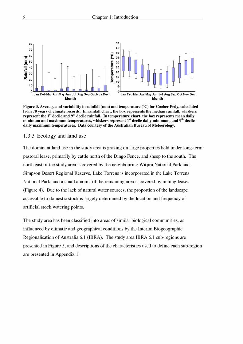
Figure 3. Average and variability in rainfall (mm) and temperature (oC) for Coober Pedy,
calculated from 70 years of climate records. In rainfall chart, the box represents the
median rainfall, whiskers represent the 1st decile and 9
th decile rainfall. In temperature
chart, the box represents mean daily minimum and maximum temperatures, whiskers
represent 1st decile daily minimum, and 9
th decile daily maximum temperatures. Data
courtesy of the Australian Bureau of Meteorology............................................................. 8
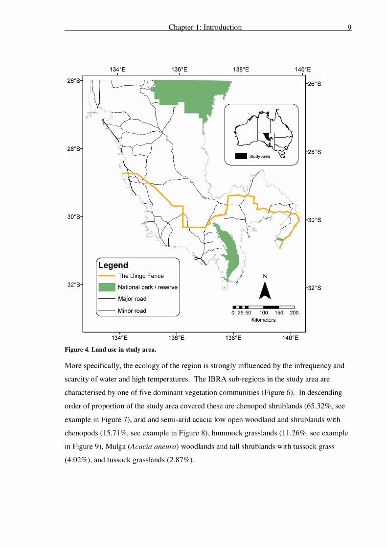
Figure 4. Land use in study area. ....................................................................................... 9
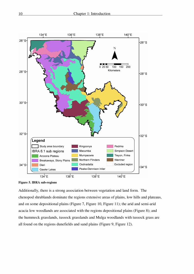
Figure 5. IBRA sub-regions .............................................................................................10
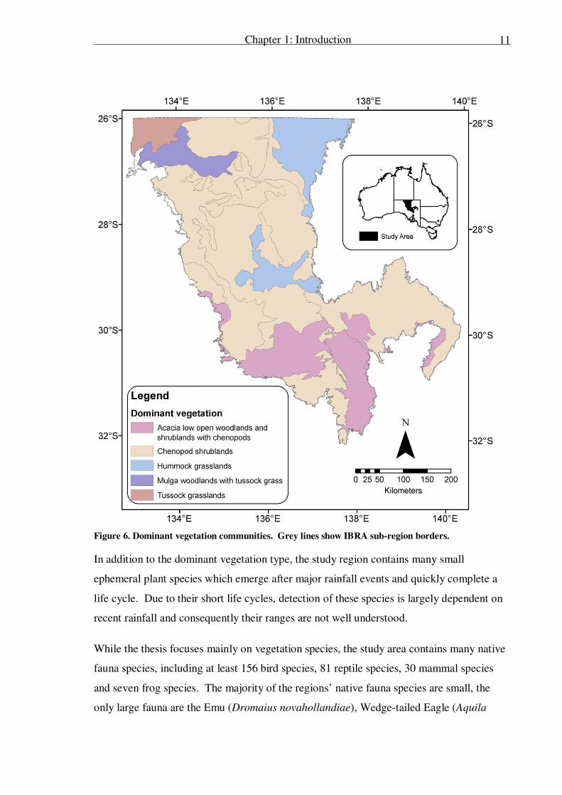
Figure 6. Dominant vegetation communities. Grey lines show IBRA sub-region borders.11
Figure 7. Chenopod shrubland. .........................................................................................14
Figure 8. Acacia low open woodland. ...............................................................................14
Figure 9. Simpson Desert. Photo courtesy of Patricia Mc. ...............................................14
Figure 10. Stony gibber, typical of Arcoona Plateau IBRA 6.1 sub-region and some parts
of other sub-regions. Photo courtesy of Patricia Mc. ........................................................14
Figure 11. Stony plains.....................................................................................................14
Figure 12. Open woodland and tussock grass along an ephemeral creek. ..........................14
Figure 13. Biological Survey of South Australia (BSSA) site locations. ...........................15
Figure 14. South Australian Pastoral Lease Assessment (SAPLA) site locations. .............16
Figure 15. Fire history in the Stony Plains IBRA, courtesy of the Department of Land
Information, Western Australia. Fires mapped from National Oceanic and Atmospheric
Administration (NOAA) Advanced Very High Resolution Radiometer (AVHRR) data. ...31
Figure 16. Study area; Interim Biogeographic Regionalisation of Australia (IBRA) sub-
regions displayed within study area. .................................................................................51
Figure 17. Study area; Interim Biogeographic Regionalisation of Australia (IBRA) sub-
regions displayed within study area. .................................................................................69
Figure 18. The relationship between rarefaction and additive partitioning. The first point
on the rarefaction curve equates to the regional average α-diversity, the final point is the γ-
diversity and the difference between the two is the β-diversity. ........................................73

List of Figures
xv
Figure 19. Sample-based rarefaction curves derived from BSSA and SAPLA data for the
Macumba IBRA 6.1 sub-region, and typical of rarefaction curves for all sub-regions. ..... 75
Figure 20. Relationship between αmax and sampling effort (BSSA R2 = 0.18; SAPLA R
2
= 0.05)............................................................................................................................. 76
Figure 21. Relationship between γmax and sampling effort (BSSA R2 = 0.91; SAPLA R
2 =
0.89) ............................................................................................................................. 77
Figure 22. Relationship between γ50 and sampling effort (BSSA R2 = 0.62; SAPLA R
2 =
0.44) ............................................................................................................................. 78
Figure 23. Alpha (α), beta (β) and gamma (γ) diversity derived by additive partitioning of
rarefaction curves from data collected by the Biological Survey of South Australia. ........ 87
Figure 24. Elevation in the study area as recorded by the AUSLIG 9 second (~310 m)
digital elevation model (DEM). IBRA 6.1 sub-region boundaries are overlain for
interpretation; see Figure 25 for IBRA sub-region detail. ................................................. 90
Figure 25. IBRA 6.1 sub-region name, location and extent. ............................................. 94
Figure 26. Multiple resolution valley bottom flatness (VBF) index, calculated from the
AUSLIG 9 second digital elevation model (DEM). Resolution is 325 m. ........................ 95
Figure 27. Index of total net primary production (TNPP) for the period 1990 – 2003,
derived from accumulated NDVI (ΣNDVI). Resolution is 8 km. ..................................... 97
Figure 28. Accumulated Morton’s actual evapotranspiration (AAET), interpolated from 18
climate stations surrounding the study area. Resolution is approximately 5 km. AAET is a
theoretically sound surrogate for expected primary production (EPP). ............................. 98
Figure 29. Morton’s AAET scaled with VBF to account of topographic redistribution of
rainfall and create a topographically scaled index of expected primary production (TEPP).
Resolution is 8 km. .......................................................................................................... 99
Figure 30. Surrogate 1: Index of biodiversity-stress, based on the difference between net
and expected primary production. .................................................................................. 100
Figure 31. Index of average annual net primary production (mean-NPP), 1990 – 2003,
derived from 14 annual ΣNDVI images. Resolution is 8 km. ........................................ 103
Figure 32. Index of variation in annual net primary production (std-NPP), 1990 – 2003,
derived from 14 annual ΣNDVI images. Resolution is 8 km. ........................................ 104
Figure 33. Index of average annual climatically distributed rainfall use efficiency (mean-
CRUE), 1990 – 2003, derived from 14 annual CRUE images. Resolution is 8 km. ....... 105
Figure 34. Index of variation in annual climatically distributed rainfall use efficiency (std-
CRUE), 1990 – 2003, derived from 14 annual CRUE images. Resolution is 8 km. ....... 107

List of Figures
xvi
Figure 35. Index of average annual topographically scaled rainfall use efficiency (mean-
TRUE), 1990 – 2003, derived from 14 annual TRUE images. Resolution is 8 km. ........ 108
Figure 36. Index of variation in annual topographically scaled rainfall use efficiency (std-
TRUE), 1990 – 2003, derived from 14 annual TRUE images. Resolution is 8 km. ........ 110
List of Tables
xvii
List of Tables
Table 1. Population centres in study area. .......................................................................... 5
Table 2. Approximate guide to scale, sample grain and corresponding biodiversity
phenomena ...................................................................................................................... 20
Table 3. False-negative errors at BSSA site 9599............................................................. 55
Table 4. False-negative errors at BSSA site 11031 ........................................................... 56
Table 5. False-negative errors at BSSA site 10478 ........................................................... 56
Table 6. False-negative errors at BSSA site 10294 ........................................................... 57
Table 7. Species detection probabilities across all BSSA sites ......................................... 58
Table 8. Rarefaction derived α-, β- and γ-diversity at maximum sampling effort in each
IBRA 6.1 sub-region. ...................................................................................................... 76
Table 9. Rarefaction derived α-, β- and γ-diversity at maximum sampling effort in each
IBRA sub-region. ............................................................................................................ 78
Table 10. α-diversity independent of sampling effort, αmax. β- and γ-diversity corrected
for the influence of sampling effort, βsec and γsec. .......................................................... 79
Table 11. Sampling effort, woody perennial α-, β- and γ-diversity and average
biodiversity-stress index values in each IBRA 6.1 sub-region ........................................ 101
Table 12. Coefficient of determination (R2): woody perennial α-, β- and γ-diversity and
potential biodiversity stress indices................................................................................ 109

Chapter 1: Introduction
1
Chapter 1: Introduction
1.1 Motivation for the research
As we become more environmentally aware, and as economic values are placed on natural
ecosystems (Costanza et al. 1997), managers have begun to appreciate the potential cost of
allowing further degradation of our natural systems. In the Australian rangelands this has
resulted in an increased desire to monitor and manage biodiversity (Smyth et al. 2004).
Currently however, there is no suitable method for monitoring biodiversity in the extensive
Australian rangelands. Hence, there is a clear need for a tool or tools to fill this gap, to
allow monitoring of temporal and spatial change in biodiversity and therefore inform the
prioritisation of conservation goals and assist in sustainable pastoral management. But
how to best measure biodiversity?
The term biodiversity is so all-encompassing that direct measurement is not possible, and it
is necessary to measure other features which vary with biodiversity: surrogates. In the
language of Sarkar (2002), a true-surrogate represents biodiversity directly, while an
estimator-surrogate represents a true-surrogate, which in turn represents biodiversity.
Sarkar (2002) argued that species richness was one of the few suitable true-surrogates for
biodiversity because firstly, species are a well defined and understood biological category,
and secondly, species richness is measurable. However, measuring total species richness
over the entire rangelands is impractical and we therefore desire a surrogate of total species
richness, or an estimator-surrogate for biodiversity.
Thus the estimator-surrogate we seek must co-vary with total species-richness, and while
the evidence for cross-taxon surrogates is equivocal, there is significant supporting
evidence. At broad scales the species-richness of many phylogenetic groups is determined
by climatic variables: trees (Currie and Paquin 1987; O'Brien 1993; O'Brien 1998; O'Brien
et al. 2000); vascular plants (Venevsky and Venevskaia 2005); mammals (Badgley and
Fox 2000); butterflies (Hawkins and Porter 2003; Hawkins and Porter 2003); and bird
species (Hawkins et al. 2003). The species-richness of each of these groups varies in
response to similar environmental variables, and we hypothesise that the species-richness
Chapter 1: Introduction
2
of one of these groups, woody plants, is an estimator-surrogate for biodiversity. This use
of cross-taxon biodiversity surrogates is supported by the meta-analysis of 27 biodiversity
studies by Rodrigues and Brooks (2007).
While currently there are no methods of measuring or monitoring biodiversity in extensive
areas such as the Australian rangelands, historically traditional field-based methods such as
quadrat surveys have collected flora and fauna species data. However, it would be
prohibitively expensive and time consuming to use field-based surveys to map the majority
of variation in species across the Australian rangelands once, let alone regularly as required
by a monitoring program.
Therefore, field surveys are unsuitable for measuring and/or monitoring biodiversity in the
Australian rangelands for several reasons. Field surveys are not capable of collecting data
at a similar scale to the broad extent of the rangelands, the consistency of their data may
vary over time, they are relatively costly, and consequently are repeated irregularly. An
alternative to these ground based measures is the use of satellite remote sensing, which
collects data that is spatially comprehensive, calibrated and therefore consistent, relatively
inexpensive, has a high temporal frequency, and is biologically relevant.
Remotely sensed data which covers the Australian rangelands is collected on a regular
basis by sensors onboard several satellites, and can be obtained for no or minimal cost.
Some individual sensors have been collecting data for years, while some series of sensors
have been collecting data for over three decades. Consequently there are now substantial
archives of remotely sensed data covering the Australian rangelands.
There is a need for a method of measuring and monitoring biodiversity in the Australian
rangelands which is not addressed by current field-based methods. Remotely sensed data
are biologically relevant, spatially-extensive, calibrated and therefore temporally
consistent. Furthermore, extensive archives of low-cost remotely sensed data exist over
the Australian rangelands. Therefore, there is a clear need to examine the potential for
remote sensing to improve biodiversity measurement and monitoring in the Australian
rangelands.
Chapter 1: Introduction
3
1.2 Thesis topic and structure
This research has the overarching goal of developing better tools for the monitoring of
biodiversity in the rangelands of Australia. Existing vegetation quadrat survey data and
remotely sensed imagery were recognised as rich sources of biologically relevant data.
The first specific aim of the thesis was to review the potential and limitations of the
vegetation quadrat survey data. This review informed the methods developed to address
the second specific aim: to derive an ecologically and mathematically sound biodiversity
index from the vegetation quadrat survey data. The final aim of the thesis was to derive
indices of biodiversity stress from the remotely sensed data. The remotely sensed indices
of biodiversity stress were evaluated against the vegetation quadrat survey data index of
biodiversity.
This thesis is structured with six chapters, some of which were written for publication as
peer-reviewed journal articles. The chapters written as articles are included as submitted,
which necessitates some repetition of material presented in the introduction and review
chapters (Chapters 1 and 2 respectively). Additionally, these articles necessarily use the
plural ‘we’, due to the contribution of co-authors. To ensure consistency this convention
has been followed in the remainder of the thesis.
The thesis begins with a general introduction and brief overview of the need for and
motivation behind this research, an outline of the structure of the thesis, and finally an
introduction to the study area (Chapter 1). Next, Chapter 2 begins with a brief explanation
of key terms and concepts which will be used throughout the rest of the thesis. This is
followed by a review of the causes of and pressures on biodiversity at broad scales, and of
current remote sensing methods of measuring and monitoring biodiversity. Finally,
Chapter 2 ends with an outline of two potential surrogates of biodiversity stress which
could conceivably be generated at little cost from a combination of satellite and climate
data.
Prior to attempting to develop a surrogate of biodiversity from the vegetation quadrat
survey data, the assumption that these data could record species richness was tested.
Chapter 3 presents the results of this analysis, submitted to Applied Vegetation Science as
Clarke, K., Lewis, M., and Ostendorf, B., ‘False negative errors in vegetation surveys’, and
Chapter 1: Introduction
4
identifies an intrinsic limitation of the vegetation quadrat survey data: false-negative errors
render it impossible to estimate species richness at the quadrat scale.
With the limitations identified, Chapter 4 develops a method for extracting an index of
biodiversity from the vegetation quadrat survey data. This article, submitted to Ecological
Indicators, as Clarke, K., Lewis, M., and Ostendorf, B, ‘Additive partitioning of
rarefaction curves: removing the influence of sampling on species-diversity in vegetation
surveys’, combines rarefaction and additive partitioning methods to allow the extraction of
an index of vegetation species diversity from the vegetation quadrat surveys, free from the
influence of sampling effort.
In Chapter 5, two theoretical surrogates of biodiversity stress are developed from a
combination of remotely sensed and climate data, and these surrogates are validated
against the index of vegetation species diversity developed in Chapter 4. Surrogate 1 is
based on the hypothesis that the difference between net primary production (NPP) and
expected primary productivity (EPP) is indicative of biodiversity stress; Surrogate 2 is
based on the hypothesis that overgrazing decreases average NPP and rainfall use efficiency
(RUE), and increases variation in NPP and RUE.
Chapter 6 reviews the findings of the research and the extent to which the aims have been
met. Key contributions to knowledge are identified, the limitations to generalisation are
clarified, and the wider implications are discussed. The thesis ends with a summary of
important areas for future research.
1.3 Study area
1.3.1 Location and infrastructure
The study was conducted in central Australia in a region stretching from the top of Spencer
Gulf in South Australia to the Northern Territory border (Figure 1). The region contains
several small towns, ranging in population from ~80 to 4000 (Table 1), and is otherwise
sparsely populated by pastoralists. The smallest towns, Lyndhurst, Marla, Marree and
Oodnadatta are resource points on some of the more travelled tracks of the region. The
town of Woomera services a defence rocket range, Coober Pedy is a centre for opal mining
and arid tourism, and Roxby Downs services the Olympic Dam copper, uranium, gold and
Chapter 1: Introduction
5
silver mine. Apart from these towns and associated mines the region contains very little
additional built infrastructure. A major sealed road runs along the western margin of the
study area, and a sparse network of minor roads spreads throughout the rest of the study
area, some sealed and some unsealed. Finally, the Dingo Fence, a pest-exclusion fence,
bisects the study area, stretching east-west just north of Coober Pedy.
Table 1. Population centres in study area. ___________________________________
Town Population (approx) Coober Pedy 1916 Lyndhurst <100
Marla 243 Marree 80 Oodnadatta 277 Roxby Downs 4000 Woomera 300 ___________________________________
1.3.2 Physical geography and climate
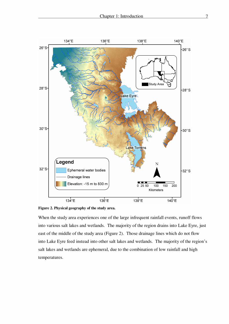
The study area is large, approximately 210,000 km2, but contains little geographic
variation. The majority of the area comprises flat or gently sloping plains, with some
notable exceptions: a line of breakaways, or mesas, stretches along the western margin of
the study area; the Simpson Desert, an area of extensive dune-fields covers the north east
of the study; and the crescent shape of Lake Torrens, a large ephemeral salt lake dominates
the south of the study area (Figure 2).
Several small wetlands and mound-springs occur around the middle north of the study
area. The mound springs are fed by an artesian aquifer, and are probably the only
permanent natural water sources in the study area. Due to their permanency these springs
support a diverse range of vegetation, invertebrates, and small mammals.
The climate of the study area is uniformly dry and hot. Average annual rainfall across the
area ranges from approximately 300 mm per annum in the south to 100 mm per annum in
the north. However, this rainfall is highly variable, and no rain or many times the average
may be received in a given month or year. The average and variation in monthly rainfall
for Coober Pedy, near the middle of the study area, is presented in Figure 3. This temporal
pattern of rainfall is typical of the entire study area.

Chapter 1: Introduction
6
Figure 1. Study area location and built infrastructure.
The average daily temperature for Coober Pedy is presented in Figure 3. The graph depicts
the mean daily minimum and maximum temperatures (box) and the 1st decile minimum
and 9th
decile maximum temperatures (oC). The average maximum temperature in January
and February is near 36 oC (96.8
oF), and daily maxima as high as 43
oC (109.4
oF) are
reasonably common.
Chapter 1: Introduction
7
Figure 2. Physical geography of the study area.
When the study area experiences one of the large infrequent rainfall events, runoff flows
into various salt lakes and wetlands. The majority of the region drains into Lake Eyre, just
east of the middle of the study area (Figure 2). Those drainage lines which do not flow
into Lake Eyre feed instead into other salt lakes and wetlands. The majority of the region’s
salt lakes and wetlands are ephemeral, due to the combination of low rainfall and high
temperatures.
Chapter 1: Introduction
8
Figure 3. Average and variability in rainfall (mm) and temperature (oC) for Coober Pedy, calculated
from 70 years of climate records. In rainfall chart, the box represents the median rainfall, whiskers
represent the 1st decile and 9
th decile rainfall. In temperature chart, the box represents mean daily
minimum and maximum temperatures, whiskers represent 1st decile daily minimum, and 9
th decile
daily maximum temperatures. Data courtesy of the Australian Bureau of Meteorology.
1.3.3 Ecology and land use
The dominant land use in the study area is grazing on large properties held under long-term
pastoral lease, primarily by cattle north of the Dingo Fence, and sheep to the south. The
north east of the study area is covered by the neighbouring Witjira National Park and
Simpson Desert Regional Reserve, Lake Torrens is incorporated in the Lake Torrens
National Park, and a small amount of the remaining area is covered by mining leases
(Figure 4). Due to the lack of natural water sources, the proportion of the landscape
accessible to domestic stock is largely determined by the location and frequency of
artificial stock watering points.
The study area has been classified into areas of similar biological communities, as
influenced by climatic and geographical conditions by the Interim Biogeographic
Regionalisation of Australia 6.1 (IBRA). The study area IBRA 6.1 sub-regions are
presented in Figure 5, and descriptions of the characteristics used to define each sub-region
are presented in Appendix 1.
Chapter 1: Introduction
9
Figure 4. Land use in study area.
More specifically, the ecology of the region is strongly influenced by the infrequency and
scarcity of water and high temperatures. The IBRA sub-regions in the study area are
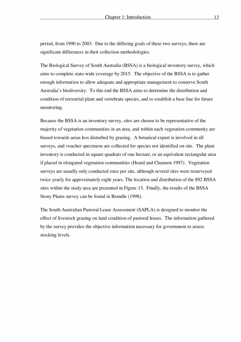
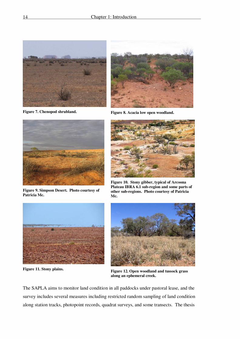
characterised by one of five dominant vegetation communities (Figure 6). In descending
order of proportion of the study area covered these are chenopod shrublands (65.32%, see
example in Figure 7), arid and semi-arid acacia low open woodland and shrublands with
chenopods (15.71%, see example in Figure 8), hummock grasslands (11.26%, see example
in Figure 9), Mulga (Acacia aneura) woodlands and tall shrublands with tussock grass
(4.02%), and tussock grasslands (2.87%).
Chapter 1: Introduction
10
Figure 5. IBRA sub-regions
Additionally, there is a strong association between vegetation and land form. The
chenopod shrublands dominate the regions extensive areas of plains, low hills and plateaus,
and on some depositional plains (Figure 7, Figure 10, Figure 11); the arid and semi-arid
acacia low woodlands are associated with the regions depositional plains (Figure 8); and
the hummock grasslands, tussock grasslands and Mulga woodlands with tussock grass are
all found on the regions dunefields and sand plains (Figure 9, Figure 12).
Chapter 1: Introduction
11
Figure 6. Dominant vegetation communities. Grey lines show IBRA sub-region borders.
In addition to the dominant vegetation type, the study region contains many small
ephemeral plant species which emerge after major rainfall events and quickly complete a
life cycle. Due to their short life cycles, detection of these species is largely dependent on
recent rainfall and consequently their ranges are not well understood.
While the thesis focuses mainly on vegetation species, the study area contains many native
fauna species, including at least 156 bird species, 81 reptile species, 30 mammal species
and seven frog species. The majority of the regions’ native fauna species are small, the
only large fauna are the Emu (Dromaius novahollandiae), Wedge-tailed Eagle (Aquila

Chapter 1: Introduction
12
audax audax), Parentie (Varanus giganteus), Red Kangaroo (Macropus rufus), and the
Dingo (Canis familiaris dingo) (Brandle 1998).
Finally, the presence of other introduced plants and animals, in addition to domestic stock,
is worth noting. Invasive introduced plant species compete with native species, and
account for 6% of all recorded plant species in the region (Brandle 1998). This
competition is strongest in wet or disturbed environments, such as along drainage lines and
close to stock watering points. Introduced camel (Camelus dromedarius) and rabbit
(Oryctolagus cuniculus) populations compete with native herbivores and domestic stock,
and put additional pressure on native vegetation. Finally, introduced fox (Vulpes vulpes)
and cat (Felis catus) populations put undue pressure on small native marsupials and
reptiles through predation.
1.3.4 Conservation objectives
The conservation objectives of the Stony Plains region are influenced by two somewhat
aligned goals: the outright desire to conserve the natural environment, and the desire to
maintain the capacity of natural systems to support livestock production. The South
Australian state government Strategic Plan set a ‘no species loss’ target (Government of
South Australia 2007), which acknowledges the importance of conservation of natural
systems, and particularly species. In the detailed strategy document (Department for
Environment and Heritage 2007) it is acknowledged that there is currently inadequate
understanding of the distribution and status of many South Australian species, and a need
for inventory and monitoring of native species for conservation. Concurrently, the
Pastoral Land Management and Conservation Act (1989) requires that the pastoral leases
which make up the majority of northern South Australia are managed sustainably, and
provides a mandate to monitor the pastoral leases to ensure this requirement is met.
The monitoring required to meet these two targets is currently performed by two
vegetation quadrat surveys, which collect vegetation species information in the study area:
the Biological Survey of South Australia (BSSA), and the South Australian Pastoral Lease
Assessment (SAPLA). These surveys provide the best quality field data for the study area,
and the analyses in this thesis examine data collected by these surveys over a 14 year
Chapter 1: Introduction
13
period, from 1990 to 2003. Due to the differing goals of these two surveys, there are
significant differences in their collection methodologies.
The Biological Survey of South Australia (BSSA) is a biological inventory survey, which
aims to complete state-wide coverage by 2015. The objective of the BSSA is to gather
enough information to allow adequate and appropriate management to conserve South
Australia’s biodiversity. To this end the BSSA aims to determine the distribution and
condition of terrestrial plant and vertebrate species, and to establish a base line for future
monitoring.
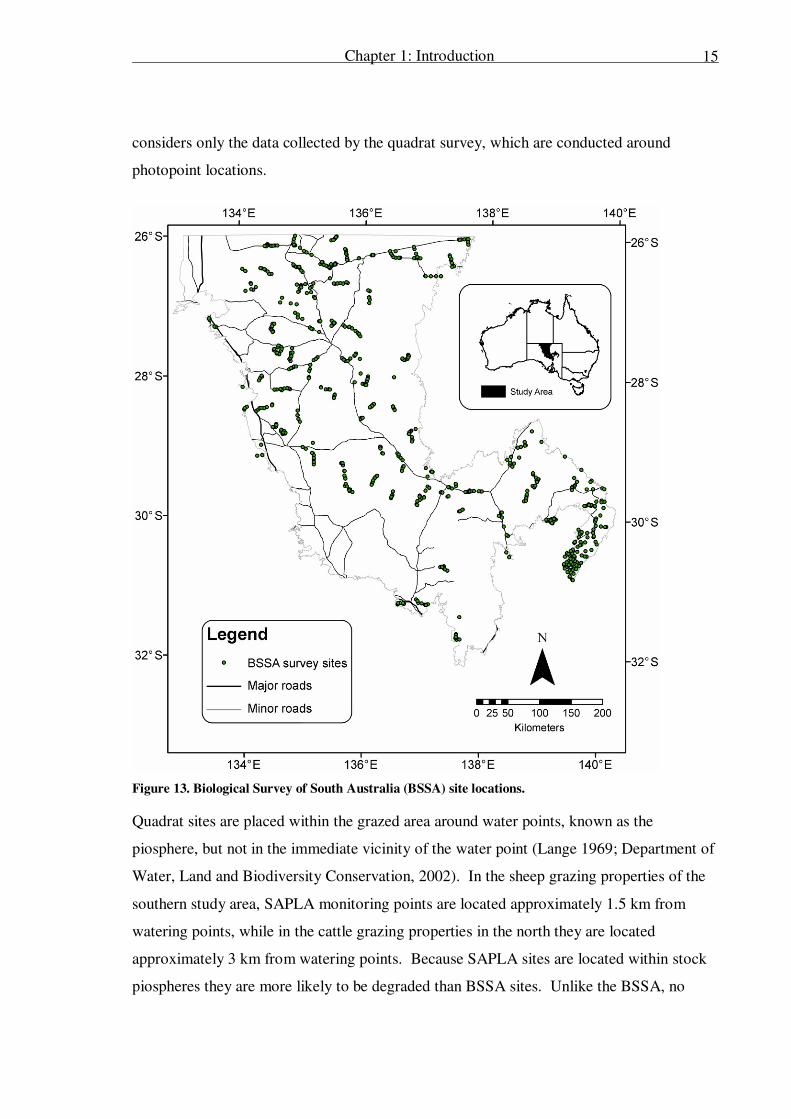
Because the BSSA is an inventory survey, sites are chosen to be representative of the
majority of vegetation communities in an area, and within each vegetation community are
biased towards areas less disturbed by grazing. A botanical expert is involved in all
surveys, and voucher specimens are collected for species not identified on site. The plant
inventory is conducted in square quadrats of one hectare, or an equivalent rectangular area
if placed in elongated vegetation communities (Heard and Channon 1997). Vegetation
surveys are usually only conducted once per site, although several sites were resurveyed
twice yearly for approximately eight years. The location and distribution of the 892 BSSA
sites within the study area are presented in Figure 13. Finally, the results of the BSSA
Stony Plains survey can be found in Brandle (1998).
The South Australian Pastoral Lease Assessment (SAPLA) is designed to monitor the
effect of livestock grazing on land condition of pastoral leases. The information gathered
by the survey provides the objective information necessary for government to assess
stocking levels.
Chapter 1: Introduction
14
Figure 7. Chenopod shrubland.
Figure 8. Acacia low open woodland.
Figure 9. Simpson Desert. Photo courtesy of
Patricia Mc.
Figure 10. Stony gibber, typical of Arcoona
Plateau IBRA 6.1 sub-region and some parts of
other sub-regions. Photo courtesy of Patricia Mc.
Figure 11. Stony plains.
Figure 12. Open woodland and tussock grass along an ephemeral creek.
The SAPLA aims to monitor land condition in all paddocks under pastoral lease, and the
survey includes several measures including restricted random sampling of land condition
along station tracks, photopoint records, quadrat surveys, and some transects. The thesis
Chapter 1: Introduction
15
considers only the data collected by the quadrat survey, which are conducted around
photopoint locations.
Figure 13. Biological Survey of South Australia (BSSA) site locations.
Quadrat sites are placed within the grazed area around water points, known as the
piosphere, but not in the immediate vicinity of the water point (Lange 1969; Department of
Water, Land and Biodiversity Conservation, 2002). In the sheep grazing properties of the
southern study area, SAPLA monitoring points are located approximately 1.5 km from
watering points, while in the cattle grazing properties in the north they are located
approximately 3 km from watering points. Because SAPLA sites are located within stock
piospheres they are more likely to be degraded than BSSA sites. Unlike the BSSA, no

Chapter 1: Introduction
16
botanical expert is involved with SAPLA surveys in the field. SAPLA staff conduct the
surveys and attempt to identify all vegetation species, while voucher specimens of any
unknown species are collected for later identification. An area of 100 to 200 metres radius
is surveyed at each site. Because the SAPLA is designed to monitor change in range
condition, sites are revisited at regular intervals. The location and distribution of the 1185
SAPLA sites within the study area are presented in Figure 14. The higher density of sites
in the south is noteworthy, and corresponds to the smaller paddocks associated with sheep
grazing.
Figure 14. South Australian Pastoral Lease Assessment (SAPLA) site locations.
Chapter 1: Introduction
17
1.4 References
Badgley, C. and D. L. Fox (2000) Ecological biogeography of North America mammals: species density and ecological structure in relation to environmental gradients. Journal of Biogeography 27: 1437-1467. Brandle, R., Ed. (1998) A biological survey of the Stony Deserts, South Australia, 1994 - 1997, Biological Survey and Research Section, Department of Environment, Heritage and Aboriginal Affairs & National Parks Foundation of South Australia Inc.
Costanza, R., R. d'Arge, R. de Groot, S. Farber, M. Grasso, B. Hannon, K. Limburg, S. Naeem, R. O'Neill, J. Paruelo, R. Raskin, P. C. Sutton and M. van den Belt (1997) The value of the world's ecosystem services and natural capital. Nature 387: 253-260. Currie, D. J. and V. Paquin (1987) Large-scale biogeographical patterns of species richness of trees. Nature 329: 326-331.
Department for Environment and Heritage (2007) No species loss: a nature conservation strategy for South Australia 2007 - 2017. Adelaide, Australia. DWLBC (2002) Pastoral lease assessment, technical manual for assessing land condition on pastoral leases in South Australia, 1990–2000. Adelaide, Department of Water, Land and Biodiversity Conservation, Pastoral Program, Sustainable Resources. Government of South Australia (2007) South Australia's strategic plan 2007. Adelaide.
Hawkins, B. A. and E. E. Porter (2003) Does herbivore diversity depend on plant diversity? The case of California butterflies. American Naturalist 161(1): 40-49. Hawkins, B. A. and E. E. Porter (2003) Water-energy balance and the geographic pattern of species richness of western Palearctic butterflies. Ecological Entomology 28: 678-686. Hawkins, B. A., E. E. Porter and J. A. F. Diniz-Filho (2003) Productivity and history as predictors of the latitudinal diversity gradient of terrestrial birds. Ecology 84(6): 1608-1623.
Heard, L. and B. Channon (1997) Guide to a native vegetation survey: Using the Biological Survey of South Australia. Adelaide, SA, Department of Environment and Natural Resources. Lange, R. T. (1969) The piosphere: sheep track and dung patterns. Journal of Range Management 22: 396-400. O'Brien, E. M. (1993) Climatic gradients in woody plant species richness: towards an explanation based on an analysis of Southern Africa's woody flora. Journal of Biogeography 20: 181-198.
O'Brien, E. M. (1998) Water-energy dynamics, climate, and prediction of woody plants species richness: an interim general model. Journal of Biogeography 25: 379-398. O'Brien, E. M., R. Field and R. J. Whittaker (2000) Climatic gradients in woody plant (tree and shrub) diversity: water-energy dynamics, residual variation, and topography. Oikos 89(3): 588-600. Rodrigues, A. S. L. and T. M. Brooks (2007) Shortcuts for biodiversity conservation planning: the effectiveness of
surrogates. Annual Review of Ecology, Evolution, and Systematics 38(1): 713-737. Sarkar, S. (2002) Defining "Biodiversity"; Assessing Biodiversity. The Monist 85(1): 131-155. Smyth, A. K., V. H. Chewings, G. N. Bastin, S. Ferrier, G. Manion and B. Clifford (2004) Integrating historical datasets to prioritise areas for biodiversity monitoring? Australian Rangelands Society 13th Biennial Conference: "Living in the outback", Alice Springs, Northern Territory. Venevsky, S. and I. Venevskaia (2005) Heirarchical systematic conservation planning at the national level: Identifying
national biodiversity hotspots using abiotic factors in Russia. Biological Conservation 124: 235-251.

Chapter 2: Literature review
18
Chapter 2: Literature review
2.1 Introduction
This review covers several important topics which develop the logic behind the work
conducted in this thesis. Firstly the literature on the ecological determinants of and
pressures on biodiversity is reviewed with a view to identifying potential surrogates of
biodiversity which are relevant to the study environment and measurable with remotely
sensed data. Next, current remote sensing methods of measuring or monitoring
biodiversity are reviewed. Finally, the potential biodiversity surrogates identified through
this review process are outlined.
However, specific biodiversity and scale terminology is used in the review and throughout
the thesis, and therefore this terminology will be clarified before proceeding any further.
2.1.1 Biodiversity phenomena: α-, β- and γ-diversity
Throughout this thesis the terminology of Whittaker (1972) is used to describe different
biodiversity, or more correctly species-diversity phenomena. In this terminology α-
diversity is the species richness at a site of standard size; β-diversity is the difference in
species composition between these sites; and γ-diversity is the species diversity of a region.
Thus α- and γ-diversity are absolute measures, while β-diversity is a comparative measure.
2.1.2 Scale in biodiversity studies
In studies on determinants of biodiversity in the past there seems to have been some
confusion as to whether “scale” refers to the extent of a study or the size of the samples it
uses. Because many ecological phenomena are scale dependant (Lyons and Willig 2002),
and because α-, β- and γ-diversity are often discussed in relation to scale, it is important
that the use of the term is clarified.
Whittaker et al. (2003) argue that the scale of a study is determined by the size of its
samples. The reason for this is twofold: it is not possible to examine the spatial fluctuation
of variables that change over distances smaller than the sample size; and, the effect of
Chapter 2: Literature review
19
variables that have a subtle effect over larger distances will be masked by small scale
variance if sample size is too small to capture an average of community structure at the
appropriate scale. However, many studies into biodiversity pattern have not used sampling
scales appropriate to the scale at which the variables of interest change, and this confusion
of extent and scale has needlessly confounded our understanding of broad scale patterns of
biodiversity (Whittaker et al. 2003). For the sake of clarity, this document accepts the
definition of scale given by Whittaker et al. (2003): the scale of a study is determined by
the size of it’s samples, not the extent of the study. This definition of scale is often
referred to as grain.
The general terms, micro, meso and macro scale are used frequently in the biodiversity
literature to describe the spatial scale of studies, but are almost never adequately defined.
Although there seems to be general agreement in the use of these scales at their extremes,
there is room for confusion at their boundaries. In the context of this discussion of
biodiversity we believe a rational classification of these scales can be arrived at by relating
them to the scale of variation of diversity phenomena (α-, β- and γ-diversity). Hence, we
consider studies of micro-scale variation in biodiversity to correspond to α-diversity;
studies of macro-scale variation in biodiversity correspond to γ-diversity; and the poorly-
defined middle ground of meso-scale studies of biodiversity may, depending on the
specifics of the given study, correspond to either α-, β- or γ-diversity.
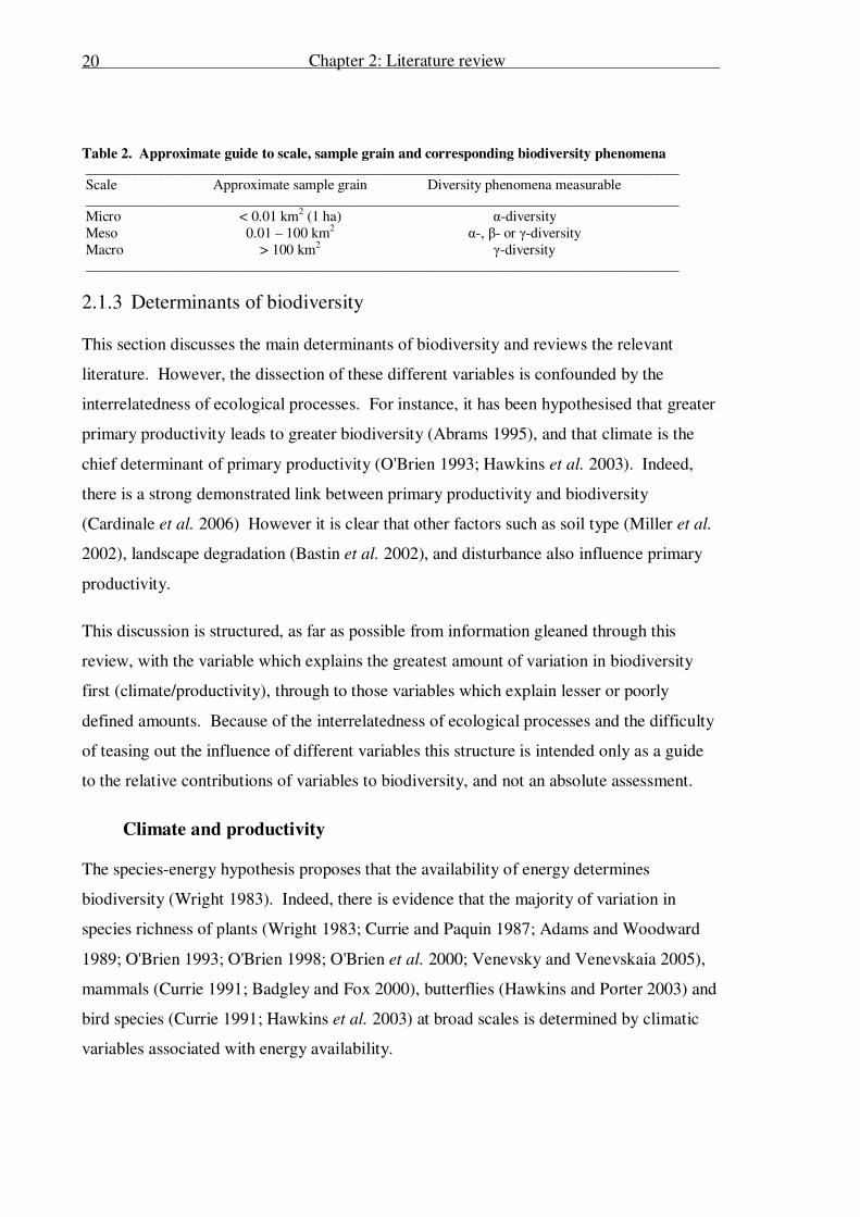
An approximate guide to the scale, sample grain appropriate to that scale, and the diversity
phenomena measurable at that scale is presented in Table 2. This table is only intended as
a guide to aid clarity and consistency in the discussion to follow, and is not intended as a
statement that the given form of biodiversity only and always varies at the defined scale. It
is acknowledged that the scale at which different types of biodiversity vary probably
changes to some extent depending on climatic and other variables. Indeed there is some
evidence that this is the case, Ohmann and Spies (1998) found that community structure
varied at finer scale in the dryer than in the wetter regions of Oregon.
Chapter 2: Literature review
20
Table 2. Approximate guide to scale, sample grain and corresponding biodiversity phenomena __________________________________________________________________________________________
Scale Approximate sample grain Diversity phenomena measurable __________________________________________________________________________________________
Micro < 0.01 km2 (1 ha) α-diversity
Meso 0.01 – 100 km2 α-, β- or γ-diversity
Macro > 100 km2 γ-diversity __________________________________________________________________________________________
2.1.3 Determinants of biodiversity
This section discusses the main determinants of biodiversity and reviews the relevant
literature. However, the dissection of these different variables is confounded by the
interrelatedness of ecological processes. For instance, it has been hypothesised that greater
primary productivity leads to greater biodiversity (Abrams 1995), and that climate is the
chief determinant of primary productivity (O'Brien 1993; Hawkins et al. 2003). Indeed,
there is a strong demonstrated link between primary productivity and biodiversity
(Cardinale et al. 2006) However it is clear that other factors such as soil type (Miller et al.
2002), landscape degradation (Bastin et al. 2002), and disturbance also influence primary
productivity.
This discussion is structured, as far as possible from information gleaned through this
review, with the variable which explains the greatest amount of variation in biodiversity
first (climate/productivity), through to those variables which explain lesser or poorly
defined amounts. Because of the interrelatedness of ecological processes and the difficulty
of teasing out the influence of different variables this structure is intended only as a guide
to the relative contributions of variables to biodiversity, and not an absolute assessment.
Climate and productivity
The species-energy hypothesis proposes that the availability of energy determines
biodiversity (Wright 1983). Indeed, there is evidence that the majority of variation in
species richness of plants (Wright 1983; Currie and Paquin 1987; Adams and Woodward
1989; O'Brien 1993; O'Brien 1998; O'Brien et al. 2000; Venevsky and Venevskaia 2005),
mammals (Currie 1991; Badgley and Fox 2000), butterflies (Hawkins and Porter 2003) and
bird species (Currie 1991; Hawkins et al. 2003) at broad scales is determined by climatic
variables associated with energy availability.

Chapter 2: Literature review
21
One of the best supported explanations for the relationship between climatic variables and
biodiversity is the Productivity Theory. This theory reasons that the greater the amount
and duration of primary productivity the greater the capacity to generate and support high
biodiversity (O'Brien 1993; Whittaker et al. 2003). However, some have questioned why
greater productivity should not simply lead to larger populations without increasing species
richness (Willig et al. 2003). Some theoretical explanations were advanced by Abrams
(1995):
1. Increased productivity increases the abundance of rare species, reducing their
extinction rates;
2. Increased productivity increases the abundance of rare resources or combinations of
resources and conditions that are required by specialists;
3. Increased productivity increases intraspecific density dependence, allowing
coexistence of species, some of which would be excluded at lower productivity;
and a fourth theoretical explanation was provided by Whittaker et al. (2003), that
4. Over large geographical areas, cells of generally high productivity will contain
scattered low productivity sites, and their species will contribute to the diversity
measured across high productivity regions.
Abrams (1995) cited evidence for each of these possible explanations, while the strong and
consistent correlations found in many studies suggest that the relationship between climate
and species richness is relatively direct (Turner 2004). Indeed, the Productivity Theory is
further supported by a recent meta-analysis of 111 biodiversity experiments which found
that, in general, the most diverse systems were also the most productive (Cardinale et al.
2006).
Thus, climatic variables determine primary productivity, which in turn determines
biodiversity. But which climatic variables are important, and specifically how do they
determine primary productivity? Primary productivity is a function of maximised water
and optimised energy, or “water-energy balance,” (O'Brien 1993; Hawkins et al. 2003).
Furthermore, measures of water-energy balance have been demonstrated to explain the
Chapter 2: Literature review
22
majority of variation in tree species richness in Africa, South America, the United States
and China (O'Brien 1998); of vascular plant species richness globally (Venevsky and
Venevskaia 2003); of butterfly species richness in western/central Europe, northern Africa
and California (Hawkins and Porter 2003; Hawkins and Porter 2003); of mammal species
richness in North America (Badgley and Fox 2000); and of bird species richness globally
(Hawkins et al. 2003).
This idea, that at the macro-scale water-energy dynamics are the primary determining
factor for species richness, was formalised by O'Brien (1998) with the Interim General
Model (IGM) of water-energy dynamics for the prediction of woody plant richness.
O'Brien (1998) found that for Africa, woody plant species richness was best described as a
function of maximised water and optimum energy, or:
Species richness = water + (energy – energy2)
Thus for a given energy level species richness increases as available water increases. The
relationship of energy to species richness is more complex. At very low and at high energy
levels species richness is zero and approaches a maximum for energy levels in between the
two extremes. This is because the availability of water for biotic processes is dependent on
energy: too little energy and water is solid, too much energy and water becomes a gas.
Finally, recent refinement of the IGM has lead to its generalisation to the theory of
‘biological relativity to water-energy dynamics’ (O'Brien 2006). This theory states that the
capacity for life to exist is determined by the capacity for liquid water to exist, and that
water-energy dynamics are a fundamental mechanism of evolution, through natural
selection. However, O'Brien (2006) make the point that at global scales water-energy
dynamics should be the primary determinant of biotic dynamics, but that the relationship
will necessarily dissolve into apparent chaos locally.
Thus, at broad scales the relationship between water-energy dynamics and species richness
has been demonstrated by significant macro-scale studies, and is relatively consistent
across the globe. The extent of the study area for the current research is large enough that
water-energy dynamics are expected to play a major role in determining regional species
richness (γ-diversity).
Chapter 2: Literature review
23
Topography
It is well established that areas of increased topographic relief are associated with
increased species richness, as compared to flatter areas (Simpson 1964; Richerson and
Lum 1980; Badgley and Fox 2000; O'Brien et al. 2000). For instance Richerson and Lum
(1980) found that topographic heterogeneity had a strong effect on patterns of flora and
fauna species richness. Diversity of flora was highest in the mountainous regions of
California and lowest in the flatter regions.
It appears that topography affects species richness in four primary ways:
1. By supporting a wider range of climatic zones and hence habitats than an
equivalent “flat” area at the same latitude. For instance a mountainous tropical
region could contain habitats ranging from tropical rainforest in the lowest regions,
through temperate and alpine forests to tundra above the snow line. Normally these
habitats would be separated by many degrees of latitude (or hundreds of
kilometres) but the high relief of the region allows communities that favour these
habitats to coexist within a relatively small spatial area (Turner 2004). This effect
is at a maximum at the equator and decreases towards the poles, i.e. mountains
from middle latitudes support temperate to tundra/snow habitats while arctic
mountainous regions only sport snow.
2. The difference in solar illumination angle between north and south facing slopes
create microclimates that would normally be found several degrees of latitude apart
(Turner 2004). This effect increases with distance from the equator.
3. According to Hewitt (1996), during climatic warming populations would move
upward in elevation toward peaks, splitting into allopatric populations. In periods
of cooling populations would then retreat down the mountains and become
sympatric again. While this process may generate species in periods of cooling it
would potentially result in extinctions in periods of warming. It is therefore not
clear that this process would necessarily lead greater species richness in areas of
high relief.
Chapter 2: Literature review
24
4. A quadrat projected onto an area of high relief will have a greater real area than one
placed over a flat area. For instance, an quadrat containing an area with an average
slope of 45o will contain approximately 40% more real area than an equivalent flat
area (Turner 2004). Thus some of the apparently greater richness in areas of high
relief is an artefact of viewing the world from a simplistic mapping perspective
which portrays the globe as a sphere (O'Brien et al. 2000; Whittaker et al. 2003;
Turner 2004).
But how significant is the effect of topography on species richness and at what scale is it
measurable? Several studies at the macro scale have found that after climate, topography
was the next strongest explanatory variable for species richness (Richerson and Lum 1980;
Currie and Paquin 1987; O'Brien et al. 2000). While some other studies have not separated
out the relative significance of the different factors, models based on topography and
climate have been demonstrated to be capable of explaining the majority of variation in the
spatial distribution of species richness (Simpson 1964; Badgley and Fox 2000; Guégan et
al. 2001; Venevsky and Venevskaia 2003).
The scale at which topography influences variation in species richness is likely to be the
scale at which the topography varies, which will depend on the particular topographic
feature. It is fair to say however that topography has been found to influence species
richness on a range of scales. Some authors have demonstrated the significant role of
topography in determining species richness at continental, or macro-scale (Simpson 1964;
O'Brien et al. 2000), while others have stated that not only does topography have an
influence on species richness at smaller scales, but also that it might be a more important
determinant of species richness than climate at these scales (Ohmann and Spies 1998).
Thus, the potential impact of topography should be considered during the development of
any biodiversity index. Specifically, it is possible that topographic variation within the
study area will play a role in determining the distribution of biodiversity.
Topographic redistribution of rainfall
Much of the precipitation in the study area occurs as infrequent high volume events. In
these events precipitation which falls on ridges and slopes, or runoff areas, is redistributed
Chapter 2: Literature review
25
by overland or sub-surface flow to areas of shallower relief, or run-on areas
(HilleRisLambers et al. 2001). Run-on areas are observed to have high primary
productivity and biodiversity (Ludwig et al. 2004), a result predicted by the previously
discussed theory of ‘biological relativity to water-energy dynamics’ (O'Brien 2006) due to
the locally increased availability of water. However, the increase in productivity and
biodiversity is the result of more than the simple topographic redistribution of
precipitation.
A positive feedback between vegetation density and water infiltration in semi-arid areas
allows greater water infiltration in more vegetated areas (HilleRisLambers et al. 2001).
Vegetation reduces raindrop impact and compaction and increases soil organic matter
content which improve water infiltration rates (Cross and Schlesinger 1999; Schlesinger et
al. 1999; Wainwright et al. 1999; Sparrow et al. 2003; Tongway et al. 2003), which in turn
allow greater vegetation growth and so on.
The combination of topographic redistribution of water, and the positive feedback between
plant density and water infiltration create regions of locally increased water availability
(above that predicted by regional precipitation records). In combination with the theory of
‘biological relativity to water-energy dynamics’ these factors explain the observed increase
in productivity and biodiversity in run-on areas.
Area and heterogeneity
The respective influences of area and heterogeneity on biodiversity are somewhat
intertwined and difficult to separate. This section provides a brief overview of the
literature relating to area and biodiversity, and habitat heterogeneity and biodiversity, and
finally a summary of the probable link between area and habitat heterogeneity.
In 1973 Terborgh suggested that the tropics support more species than other latitudinal
belts because they cover a larger area, and the two tropical belts are neighbours whereas
other latitudinal belts are separated by the tropics. Hence any species with environmental
tolerances that allow it to exist in the tropics has the potential to populate any area within
the tropics without having to cross through unfavourable latitudes, while species from
Chapter 2: Literature review
26
other latitudes are unlikely to be able to populate their corresponding latitudinal belt in the
opposite hemisphere.
Of course species cannot freely move within the global extent of an entire latitudinal belt
due to geographic obstacles. However this theory suggests, as does the Theory of Island
Biogeography (MacArthur and Wilson 1967) that diversity of species should increase as
the size of a landmass in a latitudinal band increases. This has been demonstrated to be the
case for islands (i.e. larger islands support more species than smaller comparable islands)
and there is some evidence for this effect on larger landmasses, but this theory is still
controversial and far from proven (Turner 2004). For instance Rahbek and Graves (2001)
found a trough in avian γ-diversity in central Amazonia, instead of the peak predicted by
this theory.
Alternatively, it has been suggested that areas of a given size that contain more diverse
habitats will support a greater biodiversity; this theory is sometimes referred to as a the
habitat heterogeneity hypothesis (Hawkins et al. 2003). Research in this area is strongly
related to the research into the effect of topography on species richness, since the
mechanism proposed by that work is topographic heterogeneity, rather than absolute
elevation.
Rahbek and Graves (2001) found a strong relationship between topographic heterogeneity
and species richness of birds, and O'Brien et al. (2000) found a similar relationship
between topographic heterogeneity and woody plant species richness. In the case of
riverine fish Guégan et al. (2001) demonstrated that at the macro scale the majority of
variation in species richness was determined by net primary productivity (NPP) and habitat
heterogeneity. Lastly Miller et al. (2002) found habitat heterogeneity was important at the
micro-scale for determining plant species diversity in old growth hardwood forests in the
northern USA.
The link between topographic heterogeneity and increased species richness as found in the
studies by Rahbek and Graves (2001) and O'Brien et al. (2000) has already been discussed
in the preceding section. The findings by Guégan et al. (2001) and Miller et al. (2002) do
suggest that habitat heterogeneity plays a strong role in determining the species richness of
Chapter 2: Literature review
27
riverine fish and plant species respectively. However, it is unclear how universal this
relationship is, and whether it is likely to apply within the study area.
In summary, it seems probable that the habitat heterogeneity hypothesis goes a long way to
explaining the association between area and biodiversity: larger areas will often contain
more diverse habitat, and therefore more species. Regardless, this discussion is academic
since the data available for this thesis does not cover a large enough area to test this theory.
Soil type
Since productivity plays a significant role in determining the spatial variation of
biodiversity it seems reasonable to conclude that any factor which influences productivity
might also have influence the distribution of biodiversity. Soil type is such a factor, and is
examined in this section.
In old-growth hardwood forests of northern USA Miller et al. (2002) found that species
presence and absence was strongly determined by soil type, to the point where most
species only occurred on one soil type. Additionally, many South Australian soils are
strongly associated with distinctive vegetation communities (Specht and Specht 1999).
Importantly Miller et al. (2002) found that some soil types supported communities with
greater species richness (α-diversity) than others, although this finding was not quantified.
However a study in an Amazonian rainforest (Tuomisto et al. 2003) found no relationship
between species richness and variation in soil type.
Thus, it is possible to synthesise the probable influence of soils on biodiversity from the
literature, and the influence may be different for α- and γ-diversity. The relationship of
soils and α-diversity appears relatively clear: particular vegetation communities are
strongly associated with certain soils, and some soils happen to support vegetation
communities with a higher α-diversity than other soils. However, there does not appear to
be any evidence that particular soil types consistently support greater α-diversity than
others.
The relationship of soils and γ-diversity is less clear. The literature suggests that the strong
association of particular vegetation communities with certain soils is common. This
association may have ramifications for the influence of soil heterogeneity on γ-diversity,
Chapter 2: Literature review
28
although this is open to interpretation: if different soils support different vegetation
communities with similar α-diversity, then the γ-diversity of a region would be strongly
influenced by the number of different soil types present. However, this is predicated on
the assumption that there is little overlap in the vegetation communities supported on
different soils.
To summarise, it seems probable that soil heterogeneity would influence vegetation γ-
diversity in the study area. However, due to the extent of the study area and the relatively
coarse scale of available soil maps, it may not be possible to examine the influence of soil-
heterogeneity on biodiversity.
The influence of environmental variability on speciation
Environmental variability has sometimes been postulated to have the potential to generate
the global gradient of biodiversity, and is therefore a potential determinant of biodiversity
distribution worth examining. Turner (2004) states that the balance between the rates of
speciation and extinction must determine to some extent the biodiversity of a given
community. If speciation rate is determined by generation time (and is therefore higher in
the tropics because of higher temperatures) and extinction rate is determined by
environmental fluctuations that occur in absolute time then the change in temperature from
the equator to the poles could potentially generate the latitudinal gradient of species
richness (Turner 2004).
However, there is significant evidence against the hypothesis that environmental variability
decreases biodiversity. Richerson and Lum (1980) found mean values of temperature and
precipitation to be more important for explaining biodiversity distribution than seasonality
and irregularity. This could suggest that longer-term trends in climatic variables and their
effect on the water-energy balance is a more important determinant of biodiversity than
climatic variability.
In a study of bird species Bromham and Cardillo (2003) found no evidence to support the
idea that rates of molecular evolution increase towards the tropics, one of the key
mechanisms of this theory. Willig et al. (2003) argued that the environmental variability
Chapter 2: Literature review
29
hypotheses should be discarded if studies of other taxa fail to find evidence for greater
evolutionary rates at the tropics.
Due to the relatively uniform environment of the study area (see Chapter 1, Study area),
the environmental variability hypothesis would be expected to play a minor role in
determining the distribution of biodiversity. For this reason, and due to the evidence
against the environmental variability hypothesis, this hypothesis will not be investigated
further in this thesis.
Fire
The effects of fire on biodiversity differ depending on the landscape. Vegetation cover in
the study area is so sparse that the region experiences almost no fires. This observation is
backed by the satellite fire mapping conducted by the Department of Land Information,
Western Australia which recorded few fire hotspots or scars within the study region from
1998 to 2004 (Figure 15).
However a small part of the region is covered by Acacia wooded landscapes which are
fire-prone (Hodgkinson 2002). These woodlands are characterised by dense groves of
vegetation with sparse interpatch areas; fuel loads in the interpatch areas can reach 800-
1800 kg ha-1 and up to 7000 kg ha-1 in groves. This patchy distribution of fuel results in a
high spatial variability in fire intensity; althought the low fuel load in interpatch areas can
prevent fires from spreading. Thus while these woodlands can burn, fire frequency is
typically low (Hodgkinson 2002).
Fires have different effects on different species within a landscape type, for instance, in
one case a summer fire in central Australia greatly reduced grass biomass and increased
forb biomass (Griffin and Friedel 1984). While fires cause the death of perennial plants
the new spaces within the landscape allow the germination of a new generation of
perennials. Indeed the pattern of shrub recruitment within Australian rangelands is
strongly influenced by fire (Hodgkinson 2002). Thus the small portion of the study area
which is prone to burning has evolved to cope with, and to some extent depend on fire.
Fire is likely to have neither a net positive or negative influence on biodiversity within the
study area.
Chapter 2: Literature review
30
2.1.4 Pressures on biodiversity
While there is no doubt that environmental variables play a large role in determining the
potential biodiversity of a given location, human disturbance in the form of land-use
change has been identified as the most critical driver of biodiversity loss over the next 100
years (Sala et al. 2000). Specific causes of this habitat loss include urban expansion, and
overgrazing which leads to erosion, although the former is not likely to be a significant
pressure in the South Australian rangelands. This section examines two pressures on
biodiversity, grazing induced landscape degradation, and invasion by exotic species.
Grazing induced degradation
The main pressure on biodiversity in the study area is landscape degradation, caused
primarily by the grazing of introduced stock. In healthy perennially-vegetated landscapes
vegetation occurs in patches with relatively bare inter-patch areas, with nutrients
concentrated in vegetated patches (Reynolds et al. 1997). Grazing-induced landscape
degradation, or overgrazing, causes loss of vegetation from patches, and through wind and
water erosion the loss of nutrient-rich soil and plant litter from the landscape (Shaver et al.
1991; Northrup and Brown 1999; Meadows and Hoffman 2002). Additionally, this
degradation has been demonstrated to reduce soil physical and nutrient cycling, and hence
soil fertility, and to reduce water infiltration (Schlesinger and Pilmanis 1998; Cross and
Schlesinger 1999; Tongway et al. 2003; Lechmere-Oertel et al. 2005), reducing potential
primary production.
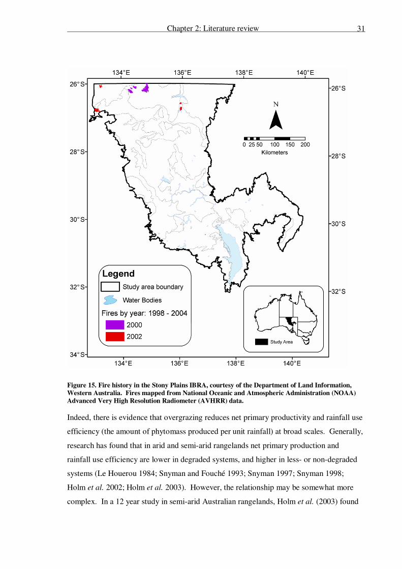
Chapter 2: Literature review
31
Figure 15. Fire history in the Stony Plains IBRA, courtesy of the Department of Land Information,
Western Australia. Fires mapped from National Oceanic and Atmospheric Administration (NOAA)
Advanced Very High Resolution Radiometer (AVHRR) data.
Indeed, there is evidence that overgrazing reduces net primary productivity and rainfall use
efficiency (the amount of phytomass produced per unit rainfall) at broad scales. Generally,
research has found that in arid and semi-arid rangelands net primary production and
rainfall use efficiency are lower in degraded systems, and higher in less- or non-degraded
systems (Le Houerou 1984; Snyman and Fouché 1993; Snyman 1997; Snyman 1998;
Holm et al. 2002; Holm et al. 2003). However, the relationship may be somewhat more
complex. In a 12 year study in semi-arid Australian rangelands, Holm et al. (2003) found

Chapter 2: Literature review
32
that net primary productivity and rainfall use efficiency were lower on average, and more
temporally variable in a degraded landscape, as compared to a non-degraded landscape. In
infrequent years of unusually high rainfall, increased primary production from ephemeral
growth resulted in net primary production on the degraded landscape similar to, or higher
than on the non-degraded landscape. This concurrent increase in temporal variability of
net primary production and rainfall use efficiency with increased degradation was also
found by Kelly and Walker (1976) in a semi-arid Zimbabwean rangeland.
Thus, there is a strong link between overgrazing and decreases in the measurable landscape
function variable, rainfall use efficiency. There is also a corresponding link between
grazing induced degradation and reduced woody perennial vegetation γ-diversity.
However, the relationship between degradation and species-diversity is not simple, and
may vary throughout the world’s rangeland systems.
In Australia, James et al. (1999) found that grazing selectively removed palatable plants
from within the piosphere, the zone of grazing influence around stock water points, locally
reducing native plant species diversity. In southern Australia, Landsberg et al. (2002)
found a grazing induced increase in plant species abundance at the local scale, and a
decrease at the regional scale. However, of the species found to increase in abundance
with proximity to water, most only exhibited this tendency on one transect in the study. Of
the plant species which exhibited trends of abundance in relation to water on two or more
transects, only two species increased with proximity to water, while four species
decreased. Thus, an alternative interpretation is that the results of Landsberg et al. (2002)
show a consistent grazing induced decline in species abundance at regional scales, a
consistent decrease in species abundance at local scales, and an inconsistent increase in
species abundance at local scales. Subsequent work by Landsberg et al. (2003) in
Australia found that ground layer (< 50 cm height) plant species which decreased in
abundance with proximity to water were significantly outnumbered by those which
increased. Importantly, Landsberg et al. (2003) also found significantly more ‘singletons’,
plants which were recorded only once out of all sites, at the sample points most remote
from water. This suggests a grazing induced loss of rare and uncommon species close to
stock water points. Landsberg et al. (2003) found no relationship between upper layer
plant species (> 50 cm height) and proximity to water. In a final Australian study,
Chapter 2: Literature review
33
McIntyre et al. (2003) found that increased grazing pressure lead to an increase in the α-
diversity of introduced or invasive species, and a decrease in native plant α-diversity.
In a hyper-arid system in northern Africa, Ali et al. (2000) demonstrated an increase in
plant α-diversity at moderate grazing pressure, and a decrease in plant α-diversity at higher
grazing pressure. In South Africa, Todd (2006) found that sustained heavy grazing in a
semi-arid system negatively impacted the plant α-diversity and structural diversity of the
landscape. Conversely, another study in South Africa found no consistent relationship
between plant species-diversity and distance from watering points (Thrash et al. 1993).
Finally, in the Mojave Desert of North America, Brooks et al. (2006) found that both
annual and perennial plant cover, and α-diversity decreased with proximity to stock
watering sites. Conversely, introduced plant abundance increased with proximity to
watering sites.
While the effects of grazing on plant species diversity across the globe may be somewhat
variable, the results within Australia appear consistent. Grazing leads to an overall
decrease in native plant α- and γ-diversity, and to an increase in invasive plant α-diversity.
Exotic species invasion
Invasion of exotic species has been identified as a serious potential threat to biodiversity in
regions with Mediterranean climates outside Europe, such as South Australia, due to their
long isolation and extensive convergent evolution (Sala et al. 2000). Exotic plant and
animal species threaten native species through competition, predation and herbivory.
Predation by the introduced fox Vulpes vulpes and cat Felis cattus is a serious pressure
native mammal populations, and has caused the decline and extinction of many Australian
mammals (Smith and Quin 1996; McKenzie et al. 2007). Additional pressure has been
placed on small Australian mammals by competition from the introduced rabbit
Oryctolagus cuniculus.
Finally, herbivory by the introduced rabit and domestic and feral stock cause grazing
induced degradation, covered in the previous section. It should also be noted that there
Chapter 2: Literature review
34
appears to be a synergy between grazing pressure and invasion of exotic vegetation
species, which is enhanced by increased grazing (McIntyre et al. 2003).
2.2 Surrogates for monitoring biodiversity
This section reviews recent approaches to measuring biodiversity, or factors which were
identified as likely to be related to biodiversity by the preceding review of the determinants
of biodiversity. Five broad categories of approach are reviewed: generalised dissimilarity
modelling; vegetation community classification; indicators of landscape condition;
measures of landscape heterogeneity; and gamma-ray spectrometry.
2.2.1 Generalised dissimilarity modelling
Smyth et al. (2007) took a risk-based approach to identifying potential biodiversity
surrogates in some of the Stony Plains of South Australia, a subset of the same area
examined in the thesis. Primary threats to biodiversity in the Stony Plains were identified,
and from these a range of relevant potential biodiversity surrogates were identified. These
included a range of topographic indices derived from a digital elevation model, as well as
the digital elevation model itself; climatic information including temperature, radiation and
moisture; Landsat TM bands 2, 3 & 4; a remotely-sensed perennial vegetation index, its
variance and contrast; gamma radiometric data; distance to water; grazing gradients, and
grazing pressure.
Generalised dissimilarity modelling (GDM) (Ferrier 2002) was employed to examine the
β-diversity of persistent native vegetation species (as a surrogate for biodiversity) in
relation to the potential biodiversity surrogates. Contrary to expectations, no relationship
was found between any of the potential biodiversity surrogates and persistent native
vegetation β-diversity.
Smyth et al. (2007) listed several potential reasons for the failure of their model, the most
significant of which were the low resolution of the climate information, and the temporal
difference between collection of the native vegetation data, and the satellite imagery
acquisition. The climate information was collected from very few stations and then
extrapolated to the whole region, and consequently varied little over the study region. The
Chapter 2: Literature review
35
vegetation data were collected primarily between 1990 and 2003, while the two satellite
images were collected in 2000 and 2002.
2.2.2 Vegetation community classification
The classification of remotely sensed imagery to map distinct vegetation communities may
be indirectly useful in the mapping and monitoring of biodiversity. For biodiversity
mapping or monitoring to be assisted by the classification of remotely sensed imagery
several factors must be demonstrated. Firstly, vegetation species must be organised into
communities, with little variation in species composition within community, and
significant differences in species composition between communities. Secondly, there must
be significant spectral differences between vegetation communities. Finally and
optionally, natural or anthropogenic disturbances which alter vegetation communities and
concurrently alter biodiversity must cause significant spectral changes. While the first
point is a widely assumed by community ecologists, the second and third points bear
illustration.
The classification of vegetation communities in arid lands is a well researched area. For
instance, Lewis (1998) used supervised classification of Landsat TM imagery to map
vegetation communities in an arid Australian chenopod shrubland similar to the study area.
The remotely sensed classes agreed strongly with community classes generated from field
sample sites. In a similar climate in a different country, Tanzania, Tobler et al. (2003)
identified 15 distinct vegetation communities through field work, and then successfully
mapped these communities through supervised classification of Landsat TM imagery.
The mapping of disturbance phenomena relevant to arid areas through remotely sensed
imagery classification is a similarly well researched area. Image classification can be used
to map fire (Verlinden and Laamanen 2005; Alo and Pontius Jr 2008), anthropogenic
vegetation clearance (Cameron and Hart 1998; Cameron et al. 2004; Alo and Pontius Jr
2008), and domestic stock grazing impact (Tobler et al. 2003). While these disturbance
phenomena operate at different scales, all have some impact on vegetation communities
and hence biodiversity.
Chapter 2: Literature review
36
Therefore the theoretical requirements are met, and the use of vegetation community
classification to assist in biodiversity mapping and monitoring is valid. However this
potential is tempered by the volume of field data required. Classification techniques
typically require extensive field data input to training procedures, and/or for validation of
classes.
2.2.3 Indicators of landscape condition: rainfall use efficiency (RUE) and net
primary productivity (NPP)
The approach of measuring landscape function or degradation does not allow us to directly
determine the biodiversity of an area, although landscape degradation leads to a loss of
resources from the system and a reduction in primary productivity. Given that primary
productivity appears to play a pivotal role in determining the biodiversity of a given
landscape or region it is logical to conclude that landscape degradation leads to a reduction
in biodiversity. Hence measures of landscape degradation allow us to monitor one of the
most significant pressures on biodiversity in the arid rangelands.
Rainfall use efficiency (RUE) and net primary productivity (NPP) have been found to
decrease as the landscape becomes more degraded (Holm et al. 2002; Holm et al. 2003),
though the relationship may not be a simple one. While one study found that degraded
landscapes always produced less phytomass and had poorer RUE (Holm et al. 2002)
another study found that degraded landscapes had lower average RUE and NPP but were
overall more variable and in fact produced higher maximum NPP in response to better than
average rainfall (Holm et al. 2003). In the case of the second study it was suggested that
the greater NPP in degraded sites was due to a freeing of resources formerly tied up in
perennial vegetation patches for use by fast growing annual species, and a lack of
competition by perennial vegetation. Interestingly Holm et al. (2002) found no difference
in the response of low-shrubland and low-woodland in terms of RUE.
The knowledge gained from these studies has been applied in the examination of the
potential for remote sensing to measure RUE and NPP as surrogates for landscape
condition (Holm et al. 2003). A model based on rainfall, landscape and NPP data collected
on-ground was used to estimate NPP and RUE from 1992 to 1999 for a large area of
Western Australia. These data were compared to estimates of NPP and RUE generated
Chapter 2: Literature review
37
from NDVI indices of the National Oceanic and Atmospheric Administration’s (NOAA)
Advanced Very High Resolution Radiometer (AVHRR) satellite imagery. There was good
agreement between ground-based and remotely sensed estimates of NPP but less
agreement between estimates of RUE (Holm et al. 2003).
In a similar study (Wessels et al. 2004) evaluated a time series of AVHRR NDVI imagery
in comparison to a ground based assessment of degradation in South Africa. Wessels et al.
(2003) found that the remotely sensed and ground-measured productivity were consistently
lower in degraded than non-degraded areas, even in times of greater than average rainfall.
The field based research to date suggests that RUE or NPP are good indicators of
landscape degradation (Holm et al. 2002). It seems probable that a measure of NPP or
RUE, or perhaps a measure of change in NPP or RUE over time could be a useful method
for measuring changes in landscape degradation and hence pressure on biodiversity in the
arid and semi-arid rangelands of Australia.
2.2.4 Measures of landscape heterogeneity
The potential for measures of landscape heterogeneity in measuring or monitoring
biodiversity has a sound grounding in ecological theory. Strong relationships have been
found between landscape heterogeneity and plant (O'Brien et al. 2000), bird (Rahbek and
Graves 2001) and riverine fish (Guégan et al. 2001) species richness. Indeed Tongway et
al. (2003) found that grazing in the Australian rangelands caused landscape degradation
which lead to homogenous landscapes close to livestock watering points while sites remote
from watering points remained more heterogeneous. This section examines two methods
of measuring landscape heterogeneity, spectral variation and landscape leakiness.
Spectral variation
The spectral variation hypothesis (SVH) (Palmer et al. 2002) takes the form: greater spatial
variation within the environment correlates with greater species richness, which in turn
correlates with greater spectral variation.
Studies examining the SVH have met with varying degrees of success ranging from no
relationship to quite strong relationships between spectral variation and species richness.

Chapter 2: Literature review
38
Two studies at the micro-scale, one in Amazonian rainforest (Tuomisto et al. 2003) and the
other in Oklahoma in the USA (Palmer et al. 2002), found no relationship between spectral
heterogeneity and species richness. Palmer et al. (2002) hypothesised that spectral
variation would be better able to predict species richness at meso- to macro-scales. In a
later test of this hypothesis Rocchini et al. (2004) examined spectral variation at two larger
scales 100m2 (still within our definition of micro-scale but larger than the sample size used
by Palmer et al. (2002)) and 1 ha (meso-scale). This study found that spectral
heterogeneity explained some variation in species richness at the micro-scale
(approximately 20%) and significantly more variation at the meso-scale (approximately
50%).
In the arid lands of Australia watering points, which are degraded by heavy stock use, were
found to have a significantly higher moving standard deviation index (MSDI) value than
non degraded areas (Jafari et al. 2008). However, the relation of MSDI to species diversity
was not examined.
The most promising study of this type found that variation in NDVI generated from
Landsat TM imagery was positively correlated with measured species richness and
explained 65% of the variation. When the variation in NDVI was combined with a
weighted abundance of vegetation types map, generated from a supervised classification, a
multiple regression indicated that these two variables significantly explained 79% of
variation in species richness of plants (Gould 2000).
Some authors have had reasonable success in mapping biodiversity with these methods.
Since this method relies on variation in measured pixel values it may be suitable for
mapping and monitoring of biodiversity. However, none of these studies have been
conducted in arid environments, and variation in biodiversity is scale dependent, as
illustrated by the findings of Rocchini et al. (2004).
However, thorough assessment of this approach to mapping biodiversity would require the
acquisition and analysis of several scales of remotely sensed imagery. The financial and
temporal cost of this analysis is beyond the scope of this thesis.

Chapter 2: Literature review
39
Landscape leakiness
Landscape leakiness is a measure of how likely a landscape is to loose resources through
wind and water erosion. While measures of landscape leakiness are similar to other
measures of landscape heterogeneity, they differ in a key respect. Unlike other landscape
heterogeneity measures, landscape leakiness is concerned with how heterogeneous the
landscape is as well as how that heterogeneity is distributed.
The measurement of landscape leakiness as a method of evaluating landscape degradation
stems from the concept that non-degraded semi-arid landscapes are characterised by a
spatial patterning of vegetation patches interspersed by almost bare soil (Aguiar and Sala
1999). Research has shown that soil attributes are better, and key resources are more
available in these vegetation patches as compared to the bare inter-patch areas (Cross and
Schlesinger 1999; Sparrow et al. 2003; Tongway et al. 2003; Ludwig et al. 2005), and it
has been demonstrated that this is a result of retention and capture of water and windborne
resources by these vegetation patches (Sparrow et al. 2003). Conversely degraded
landscapes have fewer vegetation patches (Friedel et al. 2003; Ludwig et al. 2005) and
lose, or ‘leak’ resources through wind and water erosion (Sparrow et al. 2003; Ludwig et
al. 2005). Grazing has been demonstrated to cause landscapes to become more
homogeneous, degraded and leaky, especially closer to stock watering points (Tongway et
al. 2003). It is this change from a heterogeneous landscape with many flow-obstructing
patches to a more homogenous landscape, which leaks resources, that researchers have
sought to measure.
A directional leakiness index (DLI) and a multi-directional leakiness index (MDLI) were
developed for use with high resolution airborne videography (Bastin et al. 2002; Ludwig et
al. 2002). These indices predict landscape leakiness by modelling resource flow once an
image is classified into vegetation patches (flow obstructing patches) and inter-patch area
(which promotes resource flow). However these indices do not incorporate topographic
information and are therefore limited to modelling uni-directional flow (in the case of the
DLI) or flow in a landscape with distinct vegetation bands (in the case of the MDLI).
Despite this limitation both indices were able to correctly rank several sample sites from
most to least degraded (Bastin et al. 2002; Ludwig et al. 2002).

Chapter 2: Literature review
40
While both of these indices are promising, there are a few key factors that limit their
usefulness:
1. Both indices require a user to classify the image into “patch” and “inter-patch”
areas,
2. They were developed for very high resolution imagery at the micro-scale,
3. Neither index actually models down slope flow, and
4. Neither index is comparable between images or sites due to the lack of a suitable
calibration method.
To address the first two limitations Bastin et al. (2004) developed a cover based DLI
(CDLI). The CDLI uses a measure of cover within pixels from an appropriate vegetation
index. This index is suitable for lower resolution imagery such as Landsat TM but still
does not model down slope flow and hence assumes uni-directional flow.
The remaining two limitations are critical, and prevent useful application of leakiness
indices in biodiversity monitoring. Firstly, broad scale application of leakiness models
throughout the study region would require the incorporation of a sophisticated flow model,
predicated on a suitably fine resolution digital elevation model, neither of which currently
exists. Secondly, the inability to compare leakiness values spatially and temporally renders
this method currently inappropriate for monitoring purposes.
2.2.5 Airborne gamma-ray spectrometry
Some soils and parent rocks contain radio-elements that emit characteristic gamma-rays as
they decay. Many studies have examined the possibility of recording this information with
airborne gamma-ray spectrometry (AGS) as a method of mapping soil type and
characteristics, possibly under vegetation cover (Cook et al. 1995; Bierwirth et al. 1996;
Wilford et al. 1997; Thwaites 2002)
It appears that AGS can potentially provide significant information about the variation in
lithology within an area (Wilford et al. 1997; Thwaites 2002). AGS has even been
Chapter 2: Literature review
41
demonstrated to allow mapping of some soil properties such as pH, composition and
texture (Bierwirth et al. 1996).
However, interpretation of AGS is site specific and requires detailed a priori knowledge of
the geology and/or geomorphology of a region (Bierwirth et al. 1996), or a
pedogeomorphic model (Thwaites 2002). Even with extensive ground data, interpretation
can be confounded by several factors:
• different elements have different environmental mobilities (Bierwirth et al. 1996);
• the relationship between regolith material and gamma-ray response differs from
region to region (Wilford et al. 1997);
• in some cases different regoliths have similar gamma-ray responses (Wilford et al.
1997);
• some regoliths are free of radio isotopes and hence produce no gamma-ray response
at all (Wilford et al. 1997);
• soil moisture levels can cause variation in the gamma-ray response
indistinguishable from that due to variation in the regolith (Wilford et al. 1997);
and
• the extent to which vegetation impedes measurement of gamma-ray emissions from
soil is as yet unclear.
Lastly the costs of data collection limit the use of AGS to micro and meso-scale studies.
AGS appears to show little promise in mapping or monitoring biodiversity. As previously
discussed, the ecological literature is inconclusive as to whether soil plays an important
role in determining biodiversity, interpretation of AGS requires extensive a priori
knowledge of the geomorphology of the region, and is only useful in the mapping of some
soils. Finally, Smyth et al. (2007) found no relationship between AGS and biodiversity in
the study region. Considering this, and the uncertainty surrounding whether vegetation
might impede the measurement of gamma-ray emissions, and AGS would seem to
confound any prediction of biodiversity more than it helped.
Chapter 2: Literature review
42
2.3 Summary and potential biodiversity surrogates
There are no current comprehensive methods for measuring and/or monitoring biodiversity
at the extensive scales of the Australian rangelands, remote sensing or ground based.
Through this review the determinants of and pressures on biodiversity in the study area and
at extensive scales were identified. The primary determinant of biodiversity was identified
as total primary productivity, and the balance between water and energy availability for life
was identified as the main determinant of primary productivity. The largest pressure on
biodiversity in the study area was identified as grazing induced degradation.
From the understanding of primary determinants of and pressures on biodiversity gained
through this review, and knowledge of the capabilities of remote sensing two potential
surrogates were identified. These surrogates are briefly outlined below, and developed
more thoroughly in Chapter 5.
2.3.1 Surrogate 1
The first surrogate is based on the differential effect grazing induced degradation on a
measure of expected primary productivity and a measure of actual primary productivity.
The measure of expected primary productivity is water-energy balance, and the measure of
actual primary productivity is derived from remotely sensed data.
Water-energy balance is a determinant of primary productivity, and therefore of possible
biodiversity. Because water-energy balance is a function of climatic variables it is
independent of grazing disturbance, and is therefore a measure of expected primary
productivity in the absence of disturbance.
Actual primary productivity is measured from satellite imagery through the use of
integrated normalised difference vegetation index (NDVI). This is a measure of primary
productivity after, or including the effect of grazing pressure.
It is hypothesised that the difference between expected and net primary production would
provide a measure of biodiversity-reducing disturbance in the study area.

Chapter 2: Literature review
43
2.3.2 Surrogate 2
The second surrogate is inspired by and based on the convincing link between grazing
induced degradation and the temporal variability of net primary productivity and rainfall
use efficiency. Grazing induced degradation leads to an overall decrease in native plant α-
and γ-diversity, and to an increase in invasive plant α-diversity. Additionally, over grazing
decreases average decreases mean net primary production and rainfall use efficiency, and
increases variation in primary production and rainfall use efficiency.
It is hypothesised that the average and variation in net primary productivity and rainfall use
efficiency, as measured from satellite imagery and climatic data can provide a measure of
grazing induced landscape degradation, and hence pressure on biodiversity.
Chapter 2: Literature review
44
References
Abrams, P. A. (1995) Monotonic or unimodal diversity-productivity gradients: What does competition theory predict? Ecology 76(7): 2019-2027. Adams, J. M. and F. I. Woodward (1989) Patterns in tree species richness as a test of the glacial extinction hypothesis. Nature 339: 699-701.
Aguiar, M. R. and O. E. Sala (1999) Patch structure, dynamics and implications for the functioning of arid ecosystems. Trends in Ecology and Evolution 14: 273-277. Ali, M. M., G. Dickinson and K. J. Murphy (2000) Predictors of plant diversity in a hyperarid desert wadi ecosystem. Journal of Arid Environments 45: 215-230. Alo, C. A. and R. G. Pontius Jr (2008) Identifying systematic land-cover transitions using remote sensing and GIS: the fate of forests inside and outside protected areas of Southwestern Ghana. Environment and Planning B: Planning and
Design 35: 280-295. Badgley, C. and D. L. Fox (2000) Ecological biogeography of North America mammals: species density and ecological structure in relation to environmental gradients. Journal of Biogeography 27: 1437-1467. Bastin, G. N., J. A. Ludwig, R. W. Eager, V. H. Chewings and A. C. Liedloff (2002) Indicators of landscape function: comparing patchiness metrics using remotely-sensed data from rangelands. Ecological Indicators 1: 247-260. Bastin, G. N., J. A. Ludwig, R. W. Eager, A. C. Liedloff and V. H. Chewings (2004) Indices for assessing landscape
leakiness at multiple scales. Alice Springs, CSIRO Sustainable Ecosystems. Bierwirth, P., P. Gessler and D. McKane (1996) Empirical investigation of airborne gamma-ray images as an indicator of soil properties - Wagga Wagga, NSW. 8th Australian Remote Sensing Conference. Bromham, L. and M. Cardillo (2003) Testing the link between the latitudinal gradient in species richness and rates of molecular evolution. Journal of Evolutionary Biology 16: 200-207.
Brooks, M. L., J. R. Matchett and K. H. Berry (2006) Effects of livestock watering sites on alien and native plants in the Mojave Desert, USA. Journal of Arid Environments Special Issue: Deserts of the World Part I: The changing Mojave Desert Guest Editors: K.H. Berry, R. Murphy 67(Supplement 1): 125-147. Cameron, J., S. Childs and L. Pittard-Robb (2004) "Illegal clearers busted from a great height": the use of remote sensing and GIS to manage South Australia's native vegetation. The 12th Australasian Remote Sensing and Photogrammetry Conference, Fremantle, Australia.
Cameron, J. and D. Hart (1998) Remote sensing of agricultural land cover change 1990-1995: a South Australian perspective. The 9th Australasian Sydney, Australia. Cardinale, B. J., D. S. Srivastava, J. E. Duffy, J. P. Wright, A. L. Downing, M. Sankaran and C. Jouseau (2006) Effects of biodiverstiy on the functioning of trophic groups and ecosystems. Nature 443: 989-992. Cook, S. E., R. J. Corner, P. R. Groves and G. J. Greali (1995) Use of airborne gamma radiometric data for soil mapping.
Australian Journal of Soil Research 34(1): 183-194. Cross, A. F. and W. H. Schlesinger (1999) Plant regulation of soil nutrient distribution in the northern Chihuahuan Desert. Plant Ecology 145: 11-25. Currie, D. J. (1991) Energy and large-scale patterns of animal-species and plant-species richness. American Naturalist 137(1): 27-49. Currie, D. J. and V. Paquin (1987) Large-scale biogeographical patterns of species richness of trees. Nature 329: 326-
331. Ferrier, S. (2002) Mapping spatial pattern in biodiversity for regional conservation planning: where to from here? Systematic Biology 51(2): 331-363.
Chapter 2: Literature review
45
Friedel, M. H., A. D. Sparrow, J. E. Kinloch and D. J. Tongway (2003) Degradation and recovery processes in arid grazing lands of central Australia. Part 2: vegetation. Journal of Arid Environments 55: 327-348.
Gould, W. (2000) Remote sensing of vegetation, plant species richness, and regional biodiversity hotspots. Ecological Applications 10(6): 1861-1870. Griffin, G. F. and M. H. Friedel (1984) Effects of fire on central Australian rangelands 1: fire and fuel characteristics and changes in herbage and nutrients. Australian Journal of Ecology 9(4): 381-393. Guégan, J. F., S. Lek and T. Oberdorff (2001) Energy availability and habitat heterogeneity predict global riverine fish diversity. Nature 391: 382-384.
Hawkins, B. A. and E. E. Porter (2003) Does herbivore diversity depend on plant diversity? The case of California butterflies. American Naturalist 161(1): 40-49. Hawkins, B. A. and E. E. Porter (2003) Water-energy balance and the geographic pattern of species richness of western Palearctic butterflies. Ecological Entomology 28: 678-686. Hawkins, B. A., E. E. Porter and J. A. F. Diniz-Filho (2003) Productivity and history as predictors of the latitudinal diversity gradient of terrestrial birds. Ecology 84(6): 1608-1623.
HilleRisLambers, R., M. Rietkerk, F. v. d. Bosch, H. H. T. Prins and H. d. Kroon (2001) Vegetation Pattern Formation in Semi-Arid Grazing Systems. Ecology 82(1): 50-61. Hodgkinson, K. C. (2002) Fire regimes in Acacia wooded landscapes: effects on functional processes and biological diversity. Flammable Australia: The Fire Regimes and Biodiversity of a Continent. R. A. Bradstock, J. E. Williams and A. M. Gill. Cambridge, Cambridge University Press.
Holm, A. M., S. W. Cridland and M. L. Roderick (2003) The use of time-integrated NOAA NDVI data and rainfall to assess landscape degradation in the arid shrubland of Western Australia. Remote Sensing of Environment 85: 145-158. Holm, A. M., W. A. Loneragan and M. A. Adams (2002) Do variations on a model of landscape function assist in interpreting the growth response of vegetation to rainfall in arid environments? Journal of Arid Environments 50: 23-52. Holm, A. M., I. W. Watson, W. A. Loneragan and M. A. Adams (2003) Loss of patch-scale heterogeneity on primary productivity and rainfall-use efficiency in Western Australia. Basic and Applied Ecology 4: 569-578.
Jafari, R., M. M. Lewis and B. Ostendorf (2008) An image-based diversity index for assessing land degradation in an arid environment in South Australia. Journal of Arid Environment 72: 1282-1283. James, C. D., J. Landsberg and S. R. Morton (1999) Provision of watering points in the Australian arid zone: a review of effects on biota. Journal of Arid Environments 41(1): 87-121. Kelly, R. D. and B. H. Walker (1976) The effects of different forms of land use on the ecology of a semi-arid region in
south-eastern Rhodesia. The Journal of Ecology 64(2): 553-576. Landsberg, J., C. D. James, J. Maconochie, A. O. Nicholls, J. Stol and R. Tynan (2002) Scale-related effects of grazing on native plant communities in an arid rangeland region of South Australia doi:10.1046/j.1365-2664.2002.00719.x. Journal of Applied Ecology 39(3): 427-444. Landsberg, J., C. D. James, S. R. Morton, W. J. Muller and J. Stol (2003) Abundance and composition of plant species along grazing gradients in Australian rangelands
doi:10.1111/j.1365-2664.2003.00862.x. Journal of Applied Ecology 40(6): 1008-1024. Le Houerou, H. N. (1984) Rain use efficiency: a unifying concept in arid-land ecology. Journal of Arid Environments 7: 213-247. Lechmere-Oertel, R., G., R. Cowling, M. and G. I. H. Kerley (2005) Landscape dysfunction and reduced spatial heterogeneity in soil resources and fertility in semi-arid succulent thicket, South Africa doi:10.1111/j.1442-9993.2005.01495.x. Austral Ecology 30(6): 615-624.
Lewis, M. M. (1998) Numeric classification as an aid to spectral mapping of vegetation communities. Plant Ecology 136: 133-149.
Chapter 2: Literature review
46
Ludwig, J. A., R. W. Eager, G. N. Bastin, V. H. Chewings and A. C. Liedloff (2002) A leakiness index for assessing landscape function using remote sensing. Landscape Ecology 17: 157-171.
Ludwig, J. A., D. J. Tongway, G. N. Bastin and C. D. James (2004) Monitoring ecological indicators of rangeland functional integrity and their relation to biodiversity at local to regional scales. Austral Ecology 29: 108-120. Ludwig, J. A., B. P. Wilcox, D. D. Breshears, D. J. Tongway and A. C. Imeson (2005) Vegetation patches and runoff-erosion as interacting ecohydrological processes in semiarid landscapes. Ecology 86(2): 288-297. Lyons, S. K. and M. R. Willig (2002) Species richness, latitude, and scale-sensitivity. Ecology 83(1): 47-58.
MacArthur, R. H. and E. O. Wilson (1967) The Theory of Island Biogeography. Princeton, NJ, Princeton University Press. McIntyre, S., K. M. Heard and T. G. Martin (2003) The relative importance of cattle grazing in subtropical grasslands: does it reduce or enhance plant biodiversity? Journal of Applied Ecology 40: 445-457. McKenzie, N. L., A. A. Burbidge, A. Baynes, R. N. Brereton, C. R. Dickman, G. Gordon, L. A. Gibson, P. W. Menkhorst, A. C. Robinson, M. R. Williams and J. Woinarski (2007) Analysis of factors implicated in the recent decline of Australia's mammal fauna. Journal of Biogeography 34: 597-611.
Meadows, M. E. and M. T. Hoffman (2002) The nature, extent and causes of land degradation in South Africa: legacy of the past, lessons for the future? Area 34(4): 428-437. Miller, T. F., D. J. Mladenoff and M. K. Clayton (2002) Old-growth northern hardwood forests: Spatial autocorrelation and patterns of understory vegetation. Ecological Monographs 72(4): 487-503. Northrup, B. K. and J. R. Brown (1999) Spatial distribution of soil carbon in grazed woodlands of dry tropical Australia:
tussock and inter-tussock scales. Proceedings of the VI international rangeland congress, Townsville, Australia. O'Brien, E. (2006) Biological relativity to water-energy dynamics. Journal of Biogeography 33: 1868-1888. O'Brien, E. M. (1993) Climatic gradients in woody plant species richness: towards an explanation based on an analysis of Southern Africa's woody flora. Journal of Biogeography 20: 181-198. O'Brien, E. M. (1998) Water-energy dynamics, climate, and prediction of woody plants species richness: an interim
general model. Journal of Biogeography 25: 379-398. O'Brien, E. M., R. Field and R. J. Whittaker (2000) Climatic gradients in woody plant (tree and shrub) diversity: water-energy dynamics, residual variation, and topography. Oikos 89(3): 588-600. Ohmann, J. L. and T. A. Spies (1998) Regional gradient analysis and spatial pattern of woody plant communities of Oregon forests. Ecological Monographs 68(2): 151-182.
Palmer, M. W., P. G. Earls, B. W. Hoagland, P. S. White and T. Wohlgemuth (2002) Quantitative tools for perfecting species lists. Environmetrics 13: 121-137. Rahbek, C. and G. R. Graves (2001) Multiscale assessment of patterns of avian species richness. Proceedings of the National Academy of Science, USA 98: 4534-4539. Reynolds, J. F., R. A. Virginia and W. H. Schlesinger (1997) Defining functional types for models of desertification. Plant Functional Types: their relevance to ecosystem properties and global change. T. M. Smith, H. H. Shugart and F. I.
Woodward. Cambridge, New York, Cambridge University Press: 195-216. Richerson, P. J. and K. L. Lum (1980) Patterns of plant species diversity in California: relation to weather and topography. American Naturalist 116: 504-536. Rocchini, D., A. Chiarucci and S. A. Loiselle (2004) Testing the spectral variation hypothesis by using satellite multispectral images. Acta Oecologica 26: 117-120. Sala, O. E., F. S. I. Chapin, J. J. Armesto, E. Berlow, J. Bloomfield, R. Dirzo, E. Huber-Sanwald, L. F. Huenneke, R. B.
Jackson, A. Kinzig, R. Leemans, D. M. Lodge, H. A. Mooney, M. Oesterheld, N. L. Poff, M. T. Sykes, B. H. Walker, M. Walker and D. H. Wall (2000) Global biodiversity scenarios for the year 2100. Science 287: 1770-1774.

Chapter 2: Literature review
47
Schlesinger, W. H., A. D. Abrahams, A. J. Parsons and J. Wainwright (1999) Nutrient losses in runoff from grassland and shrubland habitats in Southern New Mexico: I. rainfall simulation experiments. Biogeochemistry 45(1): 21-34.
Schlesinger, W. H. and A. M. Pilmanis (1998) Plant-soil interactions in deserts. Biogeochemistry 42: 169-187. Shaver, G. R., K. J. Nadelhoffer and A. E. Giblin (1991) Biogeochemical diversity and element transport in a heterogeneous landscape, the north slope of Alaska. Quantitative Methods in Landscape Ecology. New York, Springer-Verlag. Simpson, G. G. (1964) Species densities of North American mammals. Systematic Zoology 13(2): 57-73.
Smith, A. P. and D. G. Quin (1996) Patterns and causes of extinction and decline in Australian conilurine rodents. Biological Conservation 77(2-3): 246-267. Smyth, A. K., R. Brandle, A. Brook, V. H. Chewings, M. Fleming and J. L. Read (2007) Methods for identifying, selecting and interpreting indicators for assessing biodiversity condition in desert Australia, using the Stony Plains bioregion as a case study, Desert Knowledge Cooperative Research Centre. Snyman, H. A. (1997) The influence of range condition on the hydrological characteristics in semi-arid rangeland. The XVIII International Grassland Congress.
Snyman, H. A. (1998) Dynamics and sustainable utilization of rangeland ecosystems in arid and semi-arid climates of southern Africa. Journal of Arid Environments 39(4): 645-666. Snyman, H. A. and H. J. Fouché (1993) Estimating seasonal herbage production of a semi-arid grassland based on veld condition, rainfall, and evapotranspiration. African Journal of Range and Forage Science 10(1): 21-24. Sparrow, A. D., M. H. Friedel and D. J. Tongway (2003) Degradation and recovery processes in arid grazing lands of
central Australia. Part 3: implications at landscape scale. Journal of Arid Environments 55: 349-360. Specht, R. L. and A. Specht (1999) Australian plant communities: dynamics of structure, growth and biodiversity, Kyodo, Singapore. Terborgh, J. (1973) On the notion of favorableness in plant ecology. American Naturalist 107(956): 481-501. Thrash, I., G. K. Theron and J. d. P. Bothma (1993) Impact of water provision on herbaceous community composition in
the Kruger National Park, South Africa. African Journal of Range and Forage Science 10(1): 31-35. Thwaites, R. N. (2002) Airborne gamma-ray spectrometry in soil-landscape modelling for upland, erosional forestlands. 11th Australasian Remote Sensing and Photogrammetry Conference, Brisbane. Tobler, M. W., R. Cochard and P. J. Edwards (2003) The impact of cattle ranching on large-scale vegetation patterns in a coastal savanna in Tanzania. Journal of Applied Ecology 40(3): 430-444.
Todd, S. W. (2006) Gradients in vegetation cover, structure and species richness of Nama-Karoo shrublands in relation to distance from livestock watering points doi:10.1111/j.1365-2664.2006.01154.x. Journal of Applied Ecology 43(2): 293-304. Tongway, D. J., A. D. Sparrow and M. H. Friedel (2003) Degradation and recovery processes in arid grazing lands of central Australia. Part 1: soil and land resources. Journal of Arid Environments 55: 301-326. Tuomisto, H., A. D. Poulsen, K. Ruokolainen, R. C. Moran, C. Quintana, J. Celi and G. Canas (2003) Linking floristic
patterns with soil heterogeneity and satellite imagery in Ecuadorian Amazonia. Ecological Applications 13(2): 352-371. Turner, J. R. G. (2004) Explaining the global biodiversity gradient: energy, area, history and natural selection. Basic and Applied Ecology 5: 435-448. Venevsky, S. and I. Venevskaia (2003) Large-scale energetic and landscape factors of vegetation diversity. Ecology Letters 6(11): 1004-1016. Venevsky, S. and I. Venevskaia (2005) Heirarchical systematic conservation planning at the national level: Identifying
national biodiversity hotspots using abiotic factors in Russia. Biological Conservation 124: 235-251.
Chapter 2: Literature review
48
Verlinden, A. and R. Laamanen (2005) Long Term Fire Scar Monitoring with Remote Sensing in Northern Namibia: Relations Between Fire Frequency, Rainfall, Land Cover, Fire Management and Trees. Environmental Monitoring and Assessment 112(1-3): 231.
Wainwright, J., A. J. Parsons and A. D. Abrahams (1999) Rainfall energy under creosotebush. Journal of Arid Environments 43(2): 111-120. Wessels, K. J., S. D. Prince, P. E. Frost and D. van Zyl (2003) Assessing the effects of human-induced land degradation in the former homelands of northern South Africa with a 1 km AVHRR NDVI time-series. Remote Sensing of Environment 91: 47-67.
Wessels, K. J., S. D. Prince, P. E. Frost and D. van Zyl (2004) Assessing the effects of human-induced land degradation in the former homelands of northern South Africa with a 1 km AVHRR NDVI time-series. Remote Sensing of Environment 91: 47-67. Whittaker, R. H. (1972) Evolution and measurement of species diversity. Taxon 21(2/3): 213-251. Whittaker, R. J., K. J. Willis and R. Field (2003) Climatic-energetic explanations of diversity: a macroscopic perspective. Macroecology: concepts and consequences. T. M. Blackburn and K. J. Gaston. Oxford, Blackwell Science: 107-129.
Wilford, J. R., P. Bierwirth and M. A. Craig (1997) Application of airborne gamma-ray spectrometry in soil/regolith mapping and applied geomorphology. AGSO Journal of Australian Geology & Geophysics 17(2): 201-216. Willig, M. R., D. M. Kaufman and R. D. Stevens (2003) Latitudinal gradients of biodiversity: pattern, process, scale, and synthesis. Annual Review of Ecology and Systematics 34: 273-309. Wright, D. (1983) Species-energy theory: an extension of species-area theory. Oikos 41: 496-506.

Chapter 3: False negative errors in vegetation quadrat surveys
49
Chapter 3: False-negative errors in a survey of persistent,
highly-detectable vegetation species
Authors: Clarke, K., Lewis, M., Ostendorf, B.
Key words: false-negative errors; biological surveys; presence-absence data; perennial
vegetation
3.1 Introduction
Fauna and flora surveys collect presence-absence data for a variety of reasons, including
inventory surveying, ecological monitoring and change detection for environmental
management. The data generated by these surveys informs environmental management
and policy formation. However, errors within the data collected by these surveys are often
overlooked or ignored. One such problem present in many fauna and flora surveys is the
presence of false-negative errors; the failure to record a species which was actually present.
Several studies have examined false-negative errors in vegetation surveys and
demonstrated that both common (Kéry et al. 2006) and rare (Alexander et al. 1997; Slade
et al. 2003; Kéry et al. 2006; Regan et al. 2006) plant species are imperfectly detected with
a single survey. These studies highlight the need for mark-recapture methods in vegetation
surveys to minimise non-detection of un-common species.
However, we believe that false-negative error rates of common vegetation species are still
frequently underestimated. Only one study (Kéry et al. 2006) has examined false-negative
errors rates for common vegetation species, and that study examined only six species in the
Swiss Alps. It is necessary to examine false-negative rates of common species in other
regions to determine the breadth and severity of non-detection errors in conventional
vegetation surveys.
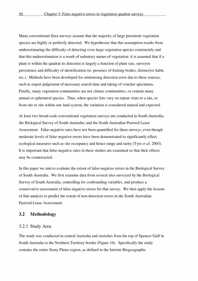
Chapter 3: False negative errors in vegetation quadrat surveys
50
Many conventional flora surveys assume that the majority of large persistent vegetation
species are highly or perfectly detected. We hypothesise that this assumption results from
underestimating the difficulty of detecting even large vegetation species consistently and
that this underestimation is a result of sedentary nature of vegetation: it is assumed that if a
plant is within the quadrat its detection is largely a function of plant size, surveyor
persistence and difficulty of identification (ie. presence of fruiting bodies, distinctive habit,
etc.). Methods have been developed for minimising detection error due to these sources,
such as expert judgement of necessary search time and taking of voucher specimens.
Finally, many vegetation communities are not climax communities, or contain many
annual or ephemeral species. Thus, when species lists vary on repeat visits to a site, or
from site to site within one land system, the variation is considered natural and expected.
At least two broad scale conventional vegetation surveys are conducted in South Australia;
the Biological Survey of South Australia; and the South Australian Pastoral Lease
Assessment. False-negative rates have not been quantified for these surveys, even though
moderate levels of false-negative errors have been demonstrated to significantly effect
ecological measures such as site occupancy and hence range and rarity (Tyre et al. 2003).
It is important that false-negative rates in these studies are examined so that their effects
may be counteracted.
In this paper we aim to evaluate the extent of false-negative errors in the Biological Survey
of South Australia. We first examine data from several sites surveyed by the Biological
Survey of South Australia, controlling for confounding variables, and produce a
conservative assessment of false-negative errors for that survey. We then apply the lessons
of that analysis to predict the extent of non-detection errors in the South Australian
Pastoral Lease Assessment.
3.2 Methodology
3.2.1 Study Area
The study was conducted in central Australia and stretches from the top of Spencer Gulf in
South Australia to the Northern Territory border (Figure 16). Specifically the study
contains the entire Stony Plains region, as defined in the Interim Biogeographic
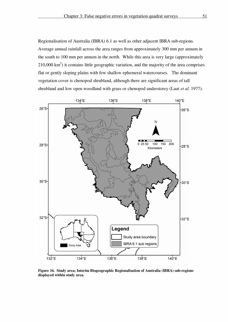
Chapter 3: False negative errors in vegetation quadrat surveys
51
Regionalisation of Australia (IBRA) 6.1 as well as other adjacent IBRA sub-regions.
Average annual rainfall across the area ranges from approximately 300 mm per annum in
the south to 100 mm per annum in the north. While this area is very large (approximately
210,000 km2) it contains little geographic variation, and the majority of the area comprises
flat or gently sloping plains with few shallow ephemeral watercourses. The dominant
vegetation cover is chenopod shrubland, although there are significant areas of tall
shrubland and low open woodland with grass or chenopod understorey (Laut et al. 1977).
Figure 16. Study area; Interim Biogeographic Regionalisation of Australia (IBRA) sub-regions
displayed within study area.
Chapter 3: False negative errors in vegetation quadrat surveys
52
Throughout the area the dominant land use is pastoral grazing of sheep in the south and
cattle in the north. However, the low rainfall of the region provides few natural watering
points for livestock. To increase the proportion of the landscape usable by livestock many
artificial water points have been established.
3.2.2 Survey data
We analysed data from two conventional vegetation surveys: the Department for
Environment and Heritage’s Biological Survey of South Australia (BSSA); and the
Department of Water Land and Biodiversity Conservation’s South Australian Pastoral
Lease Assessment (SAPLA). The majority of the data were collected over fourteen years,
from 1990 to 2003. Any data collected outside this period was excluded to ensure both
surveys covered the same time span. The two surveys have different goals and therefore
different data collection methodologies and site selection biases.
The aim of the BSSA is to create an inventory of native species and therefore sites are
generally chosen in areas less disturbed by grazing. A botanical expert participates in all
surveys, and voucher specimens are collected for species not identified on site. The plant
inventory is conducted in square quadrats of one hectare, or an equivalent rectangular area
if placed in elongated vegetation communities. Vegetation surveys are usually only
conducted once per site, although four BSSA sites were visited twice yearly for 8 years as
part of a small-mammal monitoring program. These four sites were marked with
photopoint pegs to, to aid re-location, and both fauna and flora surveys were conducted on
each visit to these four sites.
Prior to analysis, all species names in the survey data were checked for currency and
consistency and updated where necessary. With the aid of advice from the South
Australian Herbarium, species were classified as either perennial or ephemeral, where
perennials were defined as plants with an expected lifespan of three or more years in the
study area. All ephemeral plant species were excluded from the analysis for two reasons.
Firstly, most ephemeral species are physically small making them easily overlooked even
when present at a site. Secondly, ephemeral plant populations vary greatly with preceding
rain and were likely to confound the generation of species richness estimates.
Chapter 3: False negative errors in vegetation quadrat surveys
53
3.2.3 False-negative analysis
Our aim was to test the assumption that vegetation species are highly or perfectly detected
by conventional vegetation surveys. To this end we required sites with repeat surveys over
a relatively short time (MacKenzie et al. 2002; Tyre et al. 2003; Gu and Swihart 2004).
While many SAPLA sites were surveyed on multiple occasions, the majority of these
repeat surveys were separated by one or more years. In addition, all SAPLA sites are
placed within the piosphere, and therefore changes in stocking rate could result in real
changes in the species composition of a site and confound our assessment of false-negative
errors. Hence, we start our evaluation of false-negative errors in conventional vegetation
surveys with the aforementioned frequently re-surveyed BSSA sites.
Biological Survey of South Australia
Four Biological Survey of South Australia sites were visited twice yearly for eight years as
part of a small mammal monitoring program. Although the monitoring program focussed
primarily on small mammal monitoring, characterising land condition was an integral part
of that monitoring. Thorough vegetation surveys were conducted during each site survey
in order to characterise land condition. It is these data that were analysed for false-
negative errors. Detailed records of survey history allowed analysis of species
observations made by different surveyors.
Two different vegetation survey methodologies were conducted at the four sites, and the
surveys were conducted by up to six different principal surveyors. The first three surveys
at sites 11031, 10478 and 10294, and the first four surveys at site 9599 were conducted
over a 1ha area according to the standard Biological Survey methodology. Additionally,
these surveys were all conducted by one principal surveyor, experienced in rangeland
vegetation surveys, referred to hereafter as surveyor A. Subsequent visits were conducted
by several different principal surveyors (surveyors B, C, D, E and F) using a non-standard
vegetation survey methodology over a larger area: 8ha for sites 9599 and 11031; and 4ha
for sites 10478 and 10294.
The data collected by surveyors A, B and C were analysed to determine whether any false-
negative errors were made, and if so, how many. In the context of this study, a false-

Chapter 3: False negative errors in vegetation quadrat surveys
54
negative error was defined as the failure to record a species at a site during surveys
subsequent to the visit on which it was first recorded. The data collected by surveyors D,
E and F were not analysed because each surveyor conducted only one survey at each site.
The analysis attempts to control for two potentially confounding factors. Firstly, since our
aim was to extract a conservative estimate of false-negative errors. Hence, we only
included species described by BSSA staff as highly-detectable, persistent and easily
identifiable. This resulted in a list of one perennial grass and seven woody-perennial shrub
species. To emphasise the point, these species are perennial and therefore less likely to be
influenced by short-term rainfall events.
Secondly, observer skill can play a significant role in determining the number of species
recorded. A less skilled observer may fail to notice the minor taxonomic difference
between two species in a genus, artificially reducing the number of species recorded. To
control for observer skill, the above definition of false-negative error was applied
separately to the data collected by each surveyor. Hence, the recording of a species
presence by one surveyor had no bearing on the evaluation of false-negative error rate for
another surveyor. Additionally, by analysing the data collected by each surveyor
separately each analysis covers a shorter period of time which increases the validity of the
assumption of demographic closure.
After examining false-negative error rates at each site, we estimate the detection
probability of each species across all four BSSA sites. This was calculated as a proportion
of the number of times a species was detected out of the number of potential detections. It
is reasonable to calculate this statistic for the study as a whole, rather than by surveyor,
because observer skill has already been controlled for.
3.3 Results
3.3.1 Biological Survey of South Australia
The data collected by surveyors A, B and C for sites 9599, 11031, 10478 and 10294 are
presented in Tables 1, 2, 3 and 4 respectively. Where an observer failed to detect a plant
previously recorded by them at that site they were considered to have made a false-
negative error.
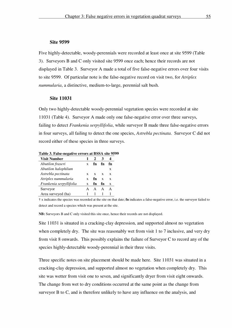
Chapter 3: False negative errors in vegetation quadrat surveys
55
Site 9599
Five highly-detectable, woody-perennials were recorded at least once at site 9599 (Table
3). Surveyors B and C only visited site 9599 once each; hence their records are not
displayed in Table 3. Surveyor A made a total of five false-negative errors over four visits
to site 9599. Of particular note is the false-negative record on visit two, for Atriplex
nummularia, a distinctive, medium-to-large, perennial salt bush.
Site 11031
Only two highly-detectable woody-perennial vegetation species were recorded at site
11031 (Table 4). Surveyor A made only one false-negative error over three surveys,
failing to detect Frankenia serpyllifolia, while surveyor B made three false-negative errors
in four surveys, all failing to detect the one species, Astrebla pectinata. Surveyor C did not
record either of these species in three surveys.
Table 3. False-negative errors at BSSA site 9599
Visit Number 1 2 3 4
Abutilon fraseri x fn fn fn
Abutilon halophilum x
Astrebla pectinata x x x x
Atriplex nummularia x fn x x
Frankenia serpyllifolia x fn fn x
Surveyor A A A A
Area surveyed (ha) 1 1 1 1
† x indicates the species was recorded at the site on that date; fn indicates a false-negative error, i.e. the surveyor failed to
detect and record a species which was present at the site.
NB: Surveyors B and C only visited this site once, hence their records are not displayed.
Site 11031 is situated in a cracking-clay depression, and supported almost no vegetation
when completely dry. The site was reasonably wet from visit 1 to 7 inclusive, and very dry
from visit 8 onwards. This possibly explains the failure of Surveyor C to record any of the
species highly-detectable woody-perennial in their three visits.
Three specific notes on site placement should be made here. Site 11031 was situated in a
cracking-clay depression, and supported almost no vegetation when completely dry. This
site was wetter from visit one to seven, and significantly dryer from visit eight onwards.
The change from wet to dry conditions occurred at the same point as the change from
surveyor B to C, and is therefore unlikely to have any influence on the analysis, and
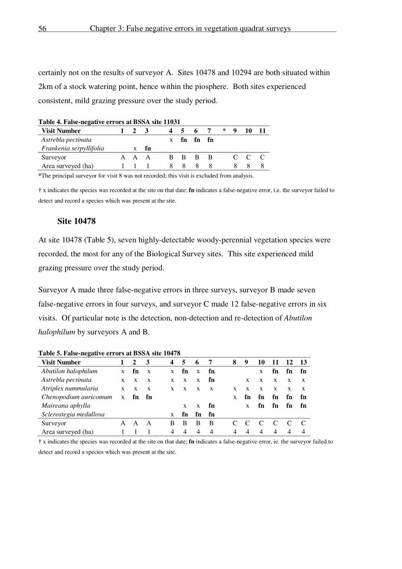
Chapter 3: False negative errors in vegetation quadrat surveys
56
certainly not on the results of surveyor A. Sites 10478 and 10294 are both situated within
2km of a stock watering point, hence within the piosphere. Both sites experienced
consistent, mild grazing pressure over the study period.
Table 4. False-negative errors at BSSA site 11031
Visit Number 1 2 3 4 5 6 7 * 9 10 11
Astrebla pectinata x fn fn fn
Frankenia serpyllifolia x fn
Surveyor A A A B B B B C C C
Area surveyed (ha) 1 1 1 8 8 8 8 8 8 8
*The principal surveyor for visit 8 was not recorded; this visit is excluded from analysis.
† x indicates the species was recorded at the site on that date; fn indicates a false-negative error, i.e. the surveyor failed to
detect and record a species which was present at the site.
Site 10478
At site 10478 (Table 5), seven highly-detectable woody-perennial vegetation species were
recorded, the most for any of the Biological Survey sites. This site experienced mild
grazing pressure over the study period.
Surveyor A made three false-negative errors in three surveys, surveyor B made seven
false-negative errors in four surveys, and surveyor C made 12 false-negative errors in six
visits. Of particular note is the detection, non-detection and re-detection of Abutilon
halophilum by surveyors A and B.
Table 5. False-negative errors at BSSA site 10478
Visit Number 1 2 3 4 5 6 7 8 9 10 11 12 13
Abutilon halophilum x fn x x fn x fn x fn fn fn
Astrebla pectinata x x x x x x fn x x x x x
Atriplex nummularia x x x x x x x x x x x x x
Chenopodium auricomum x fn fn x fn fn fn fn fn
Maireana aphylla x x fn x fn fn fn fn
Sclerostegia medullosa x fn fn fn
Surveyor A A A B B B B C C C C C C
Area surveyed (ha) 1 1 1 4 4 4 4 4 4 4 4 4 4
† x indicates the species was recorded at the site on that date; fn indicates a false-negative error, ie. the surveyor failed to
detect and record a species which was present at the site.

Chapter 3: False negative errors in vegetation quadrat surveys
57
Site 10294
Five highly-detectable woody-perennial vegetation species were recorded at Site 10294
(Table 6). As with site 10478, site 10294 experienced consistent, mild grazing pressure
over the study period.
Surveyor A made two false-negative errors in three surveys, surveyor B made four false-
negative errors in four surveys and surveyor C made seven false-negative errors in six
surveys. All three surveyors recorded, then failed to record, and then recorded again at
least one species: Surveyor A and Astrebla pectinata and Frankenia serpyllifolia; Surveyor
B and Abutilon halophilum; and Surveyor C and Frankenia serpyllifolia and Sclerostegia
medull.
Table 6. False-negative errors at BSSA site 10294
Visit Number 1 2 3 4 5 6 7 8 9 10 11 12 13
Abutilon halophilum x x x x fn x x x
Astrebla pectinata x fn x x x x x x x x x
Atriplex nummularia x x x x x x x x x x x x x
Frankenia serpyllifolia x fn x x fn fn fn x fn fn fn fn x
Sclerostegia medullosa x x x x x fn fn fn x x
Surveyor A A A B B B B C C C C C C
Area surveyed (ha) 1 1 1 4 4 4 4 4 4 4 4 4 4
† x indicates the species was recorded at the site on that date; fn indicates a false-negative error, i.e. the surveyor failed to
detect and record a species which was present at the site.
NB: Sclerostegia tennuis was only recorded on visits 8 and 16, on which Sclerostegia medullosa was recorded as absent.
Because these two species are easily confused, and were never recorded together at the site we resolved that records of
Sclerostegia tennuis were misidentifications of Sclerostegia medullosa, and re-classified them as such.
Detection Probability
Examining species detection probabilities across all sites, several species stand out for their
frequent non-detection by surveyors (Table 7). Four species have detection probabilities
less than 0.5: Frankenia serpyllifolia, Maireana aphylla, Abutilon fraseri, and
Chenopodium auricomum. However, the very low detection probability of Abutilon fraseri
is based on only four possible detections. Of particular note is the relatively-low detection
probability of 0.57 for Sclerostegia medullosa, a distinctive and relatively un-palatable
plant (Kutsche and Lay 2003).
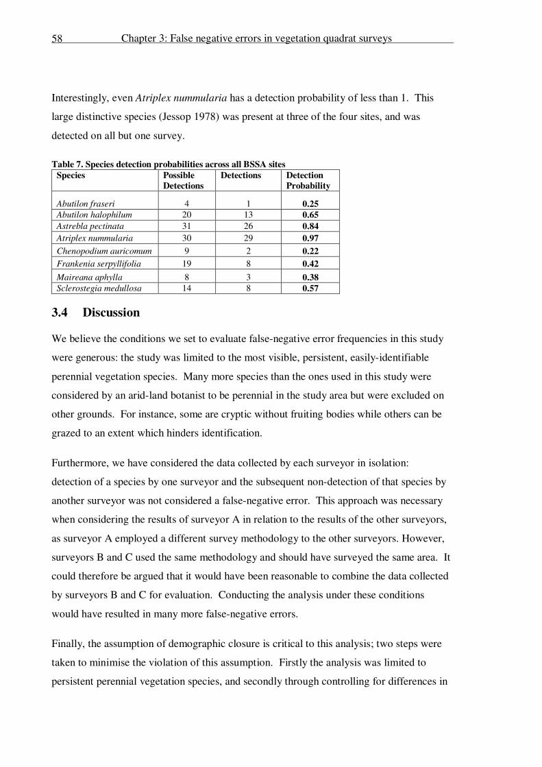
Chapter 3: False negative errors in vegetation quadrat surveys
58
Interestingly, even Atriplex nummularia has a detection probability of less than 1. This
large distinctive species (Jessop 1978) was present at three of the four sites, and was
detected on all but one survey.
Table 7. Species detection probabilities across all BSSA sites
Species Possible
Detections
Detections Detection
Probability
Abutilon fraseri 4 1 0.25
Abutilon halophilum 20 13 0.65
Astrebla pectinata 31 26 0.84
Atriplex nummularia 30 29 0.97
Chenopodium auricomum 9 2 0.22
Frankenia serpyllifolia 19 8 0.42
Maireana aphylla 8 3 0.38
Sclerostegia medullosa 14 8 0.57
3.4 Discussion
We believe the conditions we set to evaluate false-negative error frequencies in this study
were generous: the study was limited to the most visible, persistent, easily-identifiable
perennial vegetation species. Many more species than the ones used in this study were
considered by an arid-land botanist to be perennial in the study area but were excluded on
other grounds. For instance, some are cryptic without fruiting bodies while others can be
grazed to an extent which hinders identification.
Furthermore, we have considered the data collected by each surveyor in isolation:
detection of a species by one surveyor and the subsequent non-detection of that species by
another surveyor was not considered a false-negative error. This approach was necessary
when considering the results of surveyor A in relation to the results of the other surveyors,
as surveyor A employed a different survey methodology to the other surveyors. However,
surveyors B and C used the same methodology and should have surveyed the same area. It
could therefore be argued that it would have been reasonable to combine the data collected
by surveyors B and C for evaluation. Conducting the analysis under these conditions
would have resulted in many more false-negative errors.
Finally, the assumption of demographic closure is critical to this analysis; two steps were
taken to minimise the violation of this assumption. Firstly the analysis was limited to
persistent perennial vegetation species, and secondly through controlling for differences in
Chapter 3: False negative errors in vegetation quadrat surveys
59
surveyors the dataset was analysed in blocks of no more than six years. Together these
minimised the probability of local colonisation or extinction over the time span of the
study.
Even after limiting this study to the most easily-detected perennial vegetation species, and
controlling for observer skill, we revealed frequent false-negative errors by all surveyors,
at all sites, for all species. Thus, we have demonstrated in the study area that even highly
detectable vegetation species often have detection probabilities significantly less than one.
This result is interesting in the context of the collecting study: these data were the only
measure of land condition at these sites, an important part of the small-mammal monitoring
program for which this data was collected. Any measure of land-condition extracted from
this vegetation survey data which did not account for the vegetation false-negative
detection rates would be seriously flawed.
While our analysis was conducted on data collected by the Biological Survey of South
Australia (BSSA) in arid South Australia, we believe our findings have broader
implications. Surveyor A conducted the vegetation survey with the standard BSSA
methodology over the standard 1ha area. Therefore, it seems reasonable to conclude that
all BSSA flora surveys in the region contain frequent false-negative errors. These frequent
false-negative errors will limit the ends to which BSSA data can be put, and without
correction will invalidate analyses and conclusions drawn from these data.
Surveyors B and C utilised a non-standard survey methodology, so we can only draw
general conclusions from their performance. To summarise, these two trained surveyors
utilised one survey methodology to conduct repeat vegetation surveys of three sites. On all
but one occasion, when false-negative errors where possible, these surveyors recorded
false-negative errors.
Examining the results of surveyors A, B and C together, we see that three experienced
surveyors employing two different survey methodologies all frequently failed to detect
species present.
Chapter 3: False negative errors in vegetation quadrat surveys
60
3.4.1 Ramifications for similar vegetation surveys
In addition to BSSA, there are other broad scale vegetation surveys in this region that
generate vegetation data which may be used for similar purposes, and which may also
suffer from false-negative errors.
One such survey is the South Australian Pastoral Lease Assessment (SAPLA). This survey
is designed to monitor the effect of livestock grazing on land condition. Hence sample
sites are placed within the piosphere but not in the immediate vicinity of the water point.
In the sheep grazing properties of the southern study area, SAPLA monitoring points are
located approximately 1.5 km from watering points. In the cattle grazing properties in the
north of the study area SAPLA monitoring points are located approximately 3 km from
watering points. Because SAPLA sites are located within stock piospheres they are more
likely to be degraded than BSSA sites. Unlike the BSSA, no botanical expert is involved
with SAPLA surveys in the field. SAPLA staff conduct the surveys and attempt to identify
all vegetation species, while voucher specimens of any unknown species are collected for
later identification. An area of 100 to 200 metres radius is surveyed at each site. Because
the SAPLA is designed to monitor change in range condition, sites are revisited at regular
intervals. There were 1185 SAPLA sites within the study area.
It was not possible to analyse the SAPLA data in as much detail as the BSSA sites, due to
the lack of detailed site-scale information on surveyor identity and site history. However,
we argue that it is possible, and reasonable, to estimate the magnitude of false-negative
errors in SAPLA data without such an analysis. There are three key differences between
the BSSA and SAPLA surveys: area surveyed; botanical expertise; and expected grazing
pressure.
Firstly, the area surveyed by the BSSA is usually one hectare. In the BSSA sites examined
in this paper surveyor A conducted a standard survey over one hectare, while surveyors B
and C conducted surveys over four or eight hectares, depending on site. By contrast,
SAPLA sites vary between one and two hundred meters in radius, or approximately three
to 12 hectares. Assuming a fixed search time, rates of false-negative errors are likely to
increase with surveyed area, by allowing the surveyor’s less time per unit area. However,
Chapter 3: False negative errors in vegetation quadrat surveys
61
since the amount of time allocated to SAPLA site surveys is un-known, it is not possible to
estimate the effect of quadrat size differences on false-negative error rates.
Secondly, the two surveys differ in their declared level of surveyor botanical expertise.
Standard BSSA surveys include a botanical expert, while SAPLA surveys are conducted
by range monitoring professionals with some botanical experience. While the BSSA sites
examined in this study were not standard surveys, we did limit this analysis to the most
visible, persistent, easily-identifiable perennial vegetation species. Therefore, the
difference in botanical expertise is likely to result in similar or higher rates of false-
negative errors in SAPLA surveys.
Finally, BSSA and SAPLA sites are subject to different levels of grazing. The BSSA is an
inventory survey, and therefore sites are biased away from heavily grazed areas, whereas
the SAPLA is a range condition monitoring survey, and sites are placed within the
piosphere and therefore frequently grazed. Moderate to heavy grazing is likely to reduce
identifiability of plant species by removing fruiting bodies, damaging or reducing visible
leaves, and at worst reducing plants to un-identifiable stubs. Therefore, we expect the
greater grazing pressure to increase false-negative error rates at SAPLA sites.
Thus, all differences between the BSSA and SAPLA would lead us to expect higher rates
of false-negative errors in the SAPLA. False-negative errors in the SAPLA data are a
serious concern and may confound measures of range condition. For instance, the apparent
loss of one or more species from a site may simply be the result of a false-negative error,
or could be a serious result of grazing induced degradation.
3.4.2 Wider implications
Beyond the two vegetation surveys which contributed data to this study, our analysis has
implications for vegetation surveying in general. The results support the findings of Kéry
et al. (2006), that a single site-survey may miss some of the most detectable vegetation
species, and will probably miss an even greater proportion of the less detectable vegetation
species. Hence we recommend that vegetation surveys adopt measures to gauge the
detectability of species, and to correct for false-negative errors, as is already done in some
fauna surveys.

Chapter 3: False negative errors in vegetation quadrat surveys
62
The problem of false-negative errors in both flora and fauna surveying has received some
attention in recent years, and the same counter-measures are recommended. The work of
Gu and Swihart (2004) and MacKenzie et al. (2002) focused on correcting for imperfect
detection of small mammals and amphibians respectively. Both studies highlighted the
need for multiple sampling occasions at each site in estimating and correcting for non-
detection. Modelling by Tyre et al. (2003) determined that three repeat visits to a site was
the minimum required to remove bias caused by moderate levels of false-negative error in
fauna surveying, and six visits were required to effectively eliminate the effects of false
negative errors. Finally, Kéry et al. (2006) estimated the number of site visits required to
detect high and low detectability species with 95% confidence as two and four visits
respectively.
It is clear that caution is necessary when interpreting the results of conventional vegetation
surveys. We have demonstrated that the implicit assumption of perfect detection in many
vegetation surveys is invalid. Without multiple sampling occasions at each site, or some
other method for estimating species detectability, the results of vegetation surveys may
contain serious biases and inaccuracies. Without correcting for these biases and
inaccuracies ecological measures such as alpha- or beta diversity will be flawed and the
necessity of management response to an apparent species loss will be unclear.
3.5 Acknowledgements
This work was supported by funding from the Australian Desert Knowledge Cooperative
Research Centre (DKCRC) and the University of Adelaide. In addition, two DKCRC
partners provided the vegetation survey data that made this analysis possible, the South
Australian Department for Environment and Heritage supplied the Biological Survey of
South Australia data; and the South Australian Department of Water, Land and
Biodiversity Conservation supplied the South Australian Pastoral Lease Assessment data.
Special thanks to the staff of the Biological Survey of South Australia, especially Robert
Brandle, for the site and survey specific information which made this detailed analysis
possible. Also, special thanks to Helen Vonow of the South Australian State Herbarium
for help in classifying and updating vegetation species lists.
Chapter 3: False negative errors in vegetation quadrat surveys
63
3.6 References
Alexander, H. M., N. A. Slade and D. W. Kettle (1997) Application of mark-recapture models to estimation of the population size of plants. Ecology 78(4): 1230-1237. Gu, W. and R. K. Swihart (2004) Absent or undetected? Effects of non-detection of species occurrence on wildlife-habitat models. Biological Conservation 116(2): 195-203.
Jessop, J. P. (1978) Flora of South Australia. Adelaide, Government Printer. Kéry, M., J. Spillmann, C. Truong and R. Holderegger (2006) How biased are estimates of extinction probability in revisitation studies? Journal of Ecology 94: 980-986. Kutsche, F. and B. Lay (2003) Field guide to the plants of Outback South Australia, Openbook Print. Laut, P., G. Keig, M. Lazarides, E. Loffler, C. Margules, R. M. Scott and M. E. Sullivan (1977) Environments of South
Australia: Province 8, Northern Arid. Canberra, Division of Land Use Research, CSIRO: 116-168. MacKenzie, D. I., J. D. Nichols, G. B. Lachman, S. Droege, J. A. Royle and C. A. Langtimm (2002) Estimating site occupancy rates when detection probabilities are less than one. Ecology 83(8): 2248-2255. Regan, T., M. A. McCarthy, P. W. Baxter, F. D. Panetta and H. P. Possingham (2006) Optimal eradication: when to stop looking for an invasive plant. Ecology Letters 9(7): 759-766. Slade, N. A., H. M. Alexander and D. W. Kettle (2003) Estimation of population size and probabilities of survival and
detection in Mead's milkweed. Ecology 84(3): 791-797. Tyre, A. J., B. Tenhumberg, S. A. Field, D. Niejalke, K. Parris and H. P. Possingham (2003) Improving precision and reducing bias in biological surveys: estimating false-negative error rates. Ecological Applications 13(6): 1790-1801.
Chapter 4: Additive partitioning of rarefaction curves
64
Chapter 4: Additive partitioning of rarefaction curves:
removing the influence of sampling on species-diversity in
vegetation surveys
Authors: Clarke, K., Lewis, M., Ostendorf, B.
Key words: species richness, rarefaction curve, sampling effort, species diversity, scale.
4.1 Introduction
Increased interest in biodiversity conservation has resulted in government Natural
Resource Management (NRM) bodies needing improved reporting on biodiversity
condition in Australia’s rangelands (Smyth et al. 2004). Hence, there is a clear need for an
indicator of biodiversity suitable for these extensive regions. Such an indicator would
allow monitoring of temporal change in biodiversity values and therefore inform the
prioritisation of conservation goals and assist in sustainable pastoral management.
However the term biodiversity is complex and has come to encompass a great many
variables which can be associated with ecosystem health and thus identifying what to
monitor is a difficult task. To a great extent the aspect of biodiversity chosen for
monitoring will determine what is conserved, or conversely the specific conservation goal
will determine which aspect of biodiversity should be monitored.
Since it is impossible to measure biodiversity directly it is necessary to measure other
factors which vary with biodiversity, indicators or surrogates. In this paper we use the
language of Sarkar (2002) to differentiate between true-surrogates and estimator-
surrogates: a true surrogate represents biodiversity directly; an estimator-surrogate
represents a true-surrogate, which in turn represents biodiversity.
Chapter 4: Additive partitioning of rarefaction curves
65
Sarkar (2002) argued that species-richness is one of the few suitable true-surrogates for
biodiversity because 1) species are a well defined and understood category, and 2) species-
richness is measurable. Thus total species-richness is a true-surrogate for biodiversity.
However total species-richness is difficult and impractical to measure and we therefore
seek to develop a surrogate of total species-richness, or an estimator-surrogate for
biodiversity.
Thus the estimator-surrogate we seek must co-vary with total species-richness. At broad
scales the species-richness of many phylogenetic groups is determined by climatic
variables: trees (Currie and Paquin 1987; O'Brien 1993; O'Brien 1998; O'Brien et al.
2000); vascular plants (Venevsky and Venevskaia 2005); mammals (Badgley and Fox
2000); butterflies (Hawkins and Porter 2003; Hawkins and Porter 2003); and bird species
(Hawkins et al. 2003). Thus the species-richness of each of these groups varies in
response to similar environmental variables.
We propose to use the species-richness of one of these groups, woody plants, as an
estimator-surrogate for biodiversity. Indeed, the use of cross-taxon biodiversity surrogates
is supported by the meta-analysis of 27 biodiversity studies by Rodrigues and Brooks
(2007). However some woody plants have ephemeral growth styles in our study area, an
arid region of South Australia. The study area also receives localised heavy rainfall which
can cause very spatially variable growth of ephemeral species. To remove the potentially
confounding effect of variable ephemeral species occurrence we further refine our
surrogate group to woody-perennial vegetation species-richness.
Two vegetation quadrat surveys in the study area have collected vegetation data which
could potentially be used to create a measure of woody-perennial species-richness.
However, previous work by us demonstrated frequent non-detection errors within the data
collected by both surveys (Chapter 3). Therefore, raw species counts are not a valid
measure of species-richness for these datasets (Gotelli and Colwell 2001).
At this point we will clarify our use of species-richness terminology. We have proposed
measurement of the species-richness of regions, which is more accurately referred to as γ-
diversity (Whittaker 1972). In addition to examining the species within a region (γ-
diversity), we will also examine the species-richness of sites within regions (α-diversity),
Chapter 4: Additive partitioning of rarefaction curves
66
and the difference in species composition between these sites (β-diversity). It is of
particular note that these diversity measures are closely related. Whittaker (1972) notes
that the γ-diversity of a region is a function the average number of species at each site (α-
diversity) and the difference in species composition of those sites (β-diversity).
The goal of this study is to extract from the survey data an estimate of woody-perennial α-,
β- and γ-diversity which accounts for the influences of sampling effort. To this end we
turn to additive partitioning of species-diversity and rarefaction.
4.1.1 The influence of sample-grain and sampling effort
To examine variation in species-diversity across regions we must account for the
influences of site size (sample-grain) and sampling effort (Fleishman et al. 2006). The
combination of additive partitioning of species-diversity and rarefaction offers a theoretical
framework for understanding and accounting for variation in both sample-grain and
sampling effort.
Firstly, the theory of additive partitioning of species diversity provides a useful framework
for understanding the interdependent nature of α-, β- and γ-diversity, and the influence of
sample-grain and sampling effort on these forms of diversity (see Veech et al. 2002 for a
review of additive partitioning). Additionally, additive partitioning allows the expression
of α and β diversity in the same units of species richness, thus allowing direct comparison
of the two (Veech et al. 2002; Crist and Veech 2006).
As described by Crist and Veech (2006), site size, or sample-grain, will affect measured α-
diversity, as larger sites will contain more species. Spatial distribution of sites, and the
number of sites surveyed (sampling effort) will affect measured β-diversity. According to
the theory of additive partitioning of species diversity, α- and β-diversity together
determine γ-diversity by their sum, as described in Equation 1. Thus, both sample-grain
and sampling effort will determine the γ-diversity of a region.
βαγ += (1)
Secondly, the process of rarefaction is commonly used to control for variation in sampling
effort. Rarefaction is a process which calculates the average number of species represented
Chapter 4: Additive partitioning of rarefaction curves
67
by 1, 2, 3, …N samples. This is done either through Monte Carlo techniques, as we have
done, or analytically with the expressions derived by either Ugland et al. (2003) or Mao et
al. (2005) and Colwell et al. (2004). Thus rarefaction allows calculation of the expected
species-richness of a region at any level up to the maximum sampling effort in that region.
Finally, work by Crist and Veech (2006) has demonstrated a sound link between additive
partitioning of species diversity and rarefaction. The additive partitioning of species
diversity allows the extraction of α-, β- and γ-diversity from sample-based rarefaction
curves. Hence, by rarefying a group of regions to a common sampling effort and
employing the theory of additive partitioning of species diversity we can compare α-, β-
and γ-diversity at equivalent sampling efforts.
However, one final caveat needs to be made. The inherent properties of diversity are not
the only variables which affect the shape of the rarefaction curve. Different sampling
methods can favour the detection of certain species more or less, while observer ability can
have a strong influence on the number of species recorded (Boulinier et al. 1998).
Therefore, species-diversity derived from differing sampling methods should be compared
with caution.
4.1.2 Research aims
To summarise, we aim to develop a biodiversity metric free from the influence of sampling
effort, and we have argued that γ-diversity of woody-perennial vegetation is an estimator-
surrogate for biodiversity. We hypothesise that rarefaction to a common sampling effort
and extraction of α-, β- and γ-diversity through additive partitioning of species diversity
will remove the influence of sampling effort. Hence we extract α-, β- and γ-diversity from
the survey data through the use of additive partitioning of rarefaction curves. We then test
each aspect of diversity for independence from sampling effort, and develop correction
methods where necessary.
Chapter 4: Additive partitioning of rarefaction curves
68
4.2 Methods
4.2.1 Study area
The study was conducted in central Australia in an area that stretches from the top of the
Spencer Gulf in South Australia to the Northern Territory border (Figure 17). Specifically
the study included the entire Stony Plains region, as defined in the Interim Biogeographic
Regionalisation of Australia (IBRA) 6.1 as well as other adjacent IBRA sub-regions.
Average annual rainfall across the area ranges from approximately 300 mm per annum in
the south to 100 mm per annum in the north. While the study area is very large
(approximately 210,000 km2) it contains little geographic variation, and the majority of the
area is flat or gently sloping plains with few shallow ephemeral watercourses. The
majority of vegetation cover is chenopod shrubland, although there are significant areas of
tall shrubland and low open woodland with grass or chenopod understorey (Laut et al.
1977).
Throughout the area the dominant land use is pastoral grazing of sheep in the south and
cattle in the north. However, the low rainfall of the region provides few natural watering
points for livestock. To increase the proportion of the landscape usable by livestock and to
increase stocking levels many artificial water points have been established.
4.2.2 Survey data
The plant species data were derived from two conventional vegetation surveys: the
Department for Environment and Heritage’s Biological Survey of South Australia (BSSA);
and the Department of Water Land and Biodiversity Conservation’s South Australian
Pastoral Lease Assessment (SAPLA). The majority of the data were collected over
fourteen years, from 1990 to 2003. Any data collected outside this period was excluded to
ensure both surveys covered the same time span. The two surveys have different goals and
therefore different data collection methodologies and site selection biases.
The aim of the Biological Survey of South Australia (BSSA) is to create an inventory of
native species and therefore sites are generally chosen in areas less disturbed by grazing.
A botanical expert is involved in all surveys, and voucher specimens are collected for
species not identified on site. The plant inventory is conducted in square quadrats of one
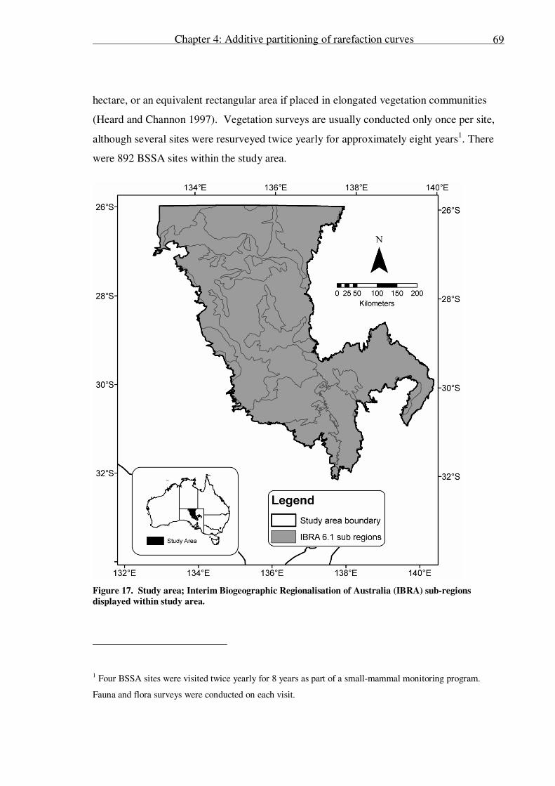
Chapter 4: Additive partitioning of rarefaction curves
69
hectare, or an equivalent rectangular area if placed in elongated vegetation communities
(Heard and Channon 1997). Vegetation surveys are usually conducted only once per site,
although several sites were resurveyed twice yearly for approximately eight years1. There
were 892 BSSA sites within the study area.
Figure 17. Study area; Interim Biogeographic Regionalisation of Australia (IBRA) sub-regions
displayed within study area.
1 Four BSSA sites were visited twice yearly for 8 years as part of a small-mammal monitoring program.
Fauna and flora surveys were conducted on each visit.
Chapter 4: Additive partitioning of rarefaction curves
70
The South Australian Pastoral Lease Assessment (SAPLA) is designed to monitor the
effect of livestock grazing on land condition. Hence sample sites are placed within the
piosphere but not in the immediate vicinity of the water point (Department of Water, Land
and Biodiversity Conservation, 2002). In the sheep grazing properties of the southern
study area, SAPLA monitoring points are located 1.5 km from watering points. In the
cattle grazing properties in the north of the study area SAPLA monitoring points are
located 3 km from watering points. Because SAPLA sites are located within stock
piospheres they are more likely to be degraded than BSSA sites. Unlike the BSSA, no
botanical expert is involved with SAPLA surveys in the field. SAPLA staff conduct the
surveys and attempt to identify all vegetation species, while voucher specimens of any
unknown species are collected for later identification. An area of 100 to 200 metres radius
is surveyed at each site. Because the SAPLA is designed to monitor change in range
condition, sites are revisited at regular intervals. There were 1185 SAPLA sites within the
study area.
Prior to analysis, all species names in the survey data were checked for currency and
consistency and updated where necessary. With the aid of advice from the South
Australian Herbarium, species were classified as either perennial or ephemeral, where
perennials were defined as plants with an expected lifespan of three or more years in the
study area. All ephemeral plant species and perennial grasses were excluded from the
analysis for two reasons. Firstly, most ephemeral species are physically small and
perennial grasses may be grazed down to vestigial stubs, making them easily overlooked
even when present at a site. Secondly, ephemeral plant populations vary greatly with
preceding rain and were likely to confound the generation of species richness estimates.
Consistency of sample-grain
The sample-grain of one of the vegetation ground surveys was consistent, while the other
varied within a small range. The sample-grain of the BSSA was consistent; a 100 m
square quadrat was surveyed at each site visit. If a square quadrat would not fit within the
surveyed vegetation community an equivalent non-square area was surveyed. The SAPLA
methodology requires that ideally a 200 m radius around sites is surveyed, although
concedes that if not possible a minimum 100m radius is acceptable. We would expect the
variation in SAPLA sample-grain will cause a similar variation in measured α-diversity.
Chapter 4: Additive partitioning of rarefaction curves
71
Therefore, we would expect the α-diversity measured by the SAPLA to vary more than the
α-diversity measured by the BSSA for the same region.
Units of aggregation and sampling effort
The vegetation data used in this study contains widely distributed quadrats surveyed at
different times. While the majority of quadrats were only surveyed once, a few quadrat-
locations were visited and surveyed on two or more occasions. We have previously
demonstrated that subsequent surveys at one quadrat-location detect previously un-
recorded species (Chapter 3, Clarke et al. submitted). Therefore, to avoid pseudo-
replication we only utilised the first quadrat-visit for each location in our analyses. Thus
our unit of sampling effort is quadrat-surveys.
This dataset was stratified by IBRA 6.1 sub-regions (Figure 17). The IBRA regions and
sub-regions have been defined based on regional and continental scale climate,
geomorphology, landform, lithology and characteristic flora and fauna-data. Rarefaction
curves were generated for each IBRA sub-region.
4.2.3 Rarefaction
We developed custom written software to calculate all rarefaction curves in this study.
Our software generates the rarefaction curve by Monte Carlo sampling sites without
replacement, rather than either of the analytical expressions derived by either Ugland et al.
(2003) or Mao et al. (2005) and Colwell et al. (2004). Our software produces rarefaction
curves identical to those produced by the analytical expression of Mao et al. (2005) and
Colwell et al. (2004) in the software package EstimateS.
Previous work has demonstrated that one of the best methods of describing rarefaction
curves is the semi-log relationship (Palmer 1990). This relationship is non-asymptotic, as
are many species and higher taxon accumulation curves (Gotelli and Colwell 2001). As
none of our rarefaction curves reach an asymptote this form of relationship is justified.
Chapter 4: Additive partitioning of rarefaction curves
72
The semi-log relationship takes the form:
bxay += )ln( (2)
Where y is the number of woody-perennial species found for given sampling effort; x is the
sampling effort; a is the log multiplier; and b is the offset.
Rarefaction curves were generated for both vegetation surveys for all IBRA sub-regions
which contained six or more quadrats. Six quadrats was an arbitrarily determined
threshold value, below which we had little confidence in generating a meaningful
rarefaction relationship.
Additive partitioning of rarefaction curves
Work by Crist and Veech (2006) has demonstrated the extraction of α-, β- and γ-diversity
from rarefaction curves through the use of additive partitioning. To illustrate with a
hypothetical region, shown in Figure 18, the α-diversity equates to the average number of
species per patch, which is mathematically identical to the first point on the rarefaction
curve. The final point on the rarefaction curve is the total number of species recorded, or
the γ-diversity. The β-diversity determines the shape of the rarefaction curve after this first
point: if sites are similar, relatively few species will be added with each additional unit of
sampling effort, producing a slowly climbing curve; if sites differ greatly in species
composite on, then the opposite is true, and the curve climbs steeply. Thus, from
diversity partitioning, the difference in species richness between the first and last points is
the total β-diversity (Crist and Veech 2006).
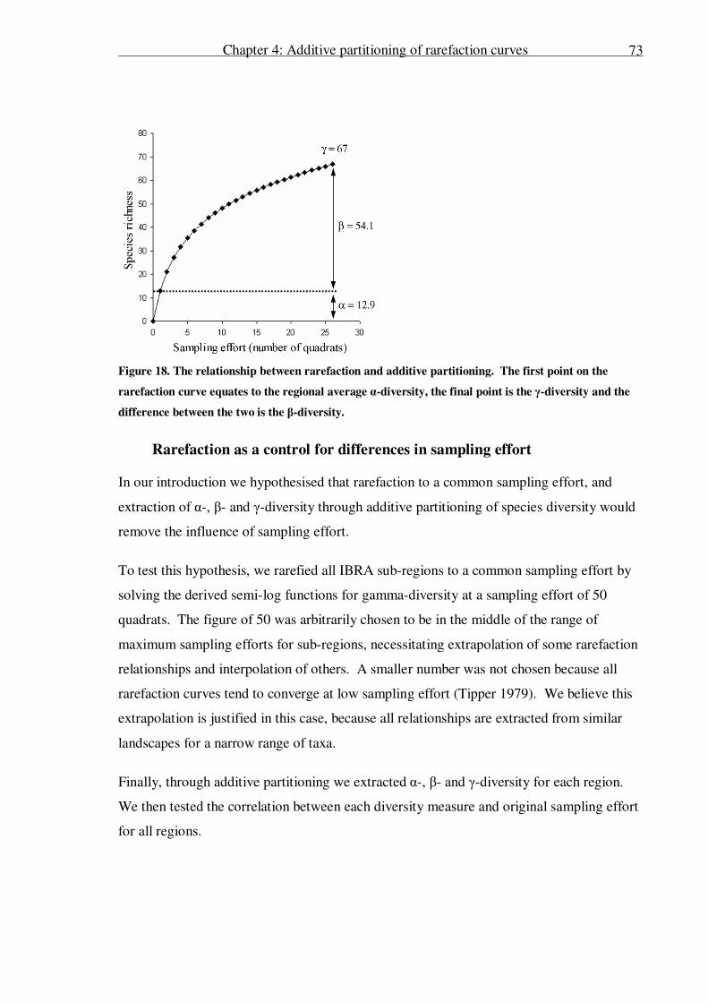
Chapter 4: Additive partitioning of rarefaction curves
73
Figure 18. The relationship between rarefaction and additive partitioning. The first point on the
rarefaction curve equates to the regional average α-diversity, the final point is the γ-diversity and the
difference between the two is the β-diversity.
Rarefaction as a control for differences in sampling effort
In our introduction we hypothesised that rarefaction to a common sampling effort, and
extraction of α-, β- and γ-diversity through additive partitioning of species diversity would
remove the influence of sampling effort.
To test this hypothesis, we rarefied all IBRA sub-regions to a common sampling effort by
solving the derived semi-log functions for gamma-diversity at a sampling effort of 50
quadrats. The figure of 50 was arbitrarily chosen to be in the middle of the range of
maximum sampling efforts for sub-regions, necessitating extrapolation of some rarefaction
relationships and interpolation of others. A smaller number was not chosen because all
rarefaction curves tend to converge at low sampling effort (Tipper 1979). We believe this
extrapolation is justified in this case, because all relationships are extracted from similar
landscapes for a narrow range of taxa.
Finally, through additive partitioning we extracted α-, β- and γ-diversity for each region.
We then tested the correlation between each diversity measure and original sampling effort
for all regions.
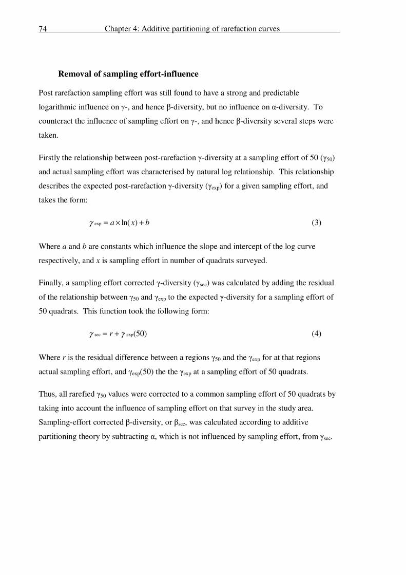
Chapter 4: Additive partitioning of rarefaction curves
74
Removal of sampling effort-influence
Post rarefaction sampling effort was still found to have a strong and predictable
logarithmic influence on γ-, and hence β-diversity, but no influence on α-diversity. To
counteract the influence of sampling effort on γ-, and hence β-diversity several steps were
taken.
Firstly the relationship between post-rarefaction γ-diversity at a sampling effort of 50 (γ50)
and actual sampling effort was characterised by natural log relationship. This relationship
describes the expected post-rarefaction γ-diversity (γexp) for a given sampling effort, and
takes the form:
bxa +×= )ln(expγ (3)
Where a and b are constants which influence the slope and intercept of the log curve
respectively, and x is sampling effort in number of quadrats surveyed.
Finally, a sampling effort corrected γ-diversity (γsec) was calculated by adding the residual
of the relationship between γ50 and γexp to the expected γ-diversity for a sampling effort of
50 quadrats. This function took the following form:
)50(expsec γγ += r (4)
Where r is the residual difference between a regions γ50 and the γexp for at that regions
actual sampling effort, and γexp(50) the the γexp at a sampling effort of 50 quadrats.
Thus, all rarefied γ50 values were corrected to a common sampling effort of 50 quadrats by
taking into account the influence of sampling effort on that survey in the study area.
Sampling-effort corrected β-diversity, or βsec, was calculated according to additive
partitioning theory by subtracting α, which is not influenced by sampling effort, from γsec.
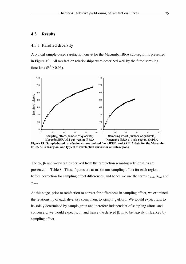
Chapter 4: Additive partitioning of rarefaction curves
75
4.3 Results
4.3.1 Rarefied diversity
A typical sample-based rarefaction curve for the Macumba IBRA sub-region is presented
in Figure 19. All rarefaction relationships were described well by the fitted semi-log
functions (R2 ≥ 0.96).
Figure 19. Sample-based rarefaction curves derived from BSSA and SAPLA data for the Macumba
IBRA 6.1 sub-region, and typical of rarefaction curves for all sub-regions.
The α-, β- and γ-diversities derived from the rarefaction semi-log relationships are
presented in Table 8. These figures are at maximum sampling effort for each region,
before correction for sampling effort differences, and hence we use the terms αmax, βmax and
γmax.
At this stage, prior to rarefaction to correct for differences in sampling effort, we examined
the relationship of each diversity component to sampling effort. We would expect αmax to
be solely determined by sample grain and therefore independent of sampling effort, and
conversely, we would expect γmax, and hence the derived βmax, to be heavily influenced by
sampling effort.
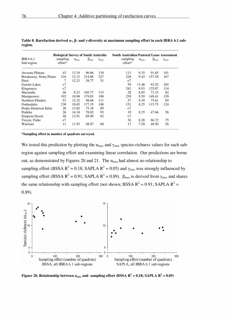
Chapter 4: Additive partitioning of rarefaction curves
76
Table 8. Rarefaction derived α-, β- and γ-diversity at maximum sampling effort in each IBRA 6.1 sub-
region. __________________________________________________________________________________________
Biological Survey of South Australia South Australian Pastoral Lease Assessment IBRA 6.1 sampling αmax βmax γmax sampling αmax βmax γmax
Sub-region effort* effort* __________________________________________________________________________________________
Arcoona Plateau 43 13.34 96.66 110 113 9.35 91.65 101 Breakaway, Stony Plains 216 12.12 214.88 227 226 9.42 157.58 167 Dieri 7 12.23 38.77 51 <7 Gawler Lakes <7 59 11.48 93.52 105 Kingoonya <7 243 8.93 125.07 134 Macumba 46 9.23 105.77 115 28 8.85 73.15 82 Murnpeowie 192 10.98 179.03 190 239 9.59 149.41 159
Northern Flinders 51 12.32 98.68 111 57 9.39 75.61 85 Oodnadatta 230 10.65 177.35 188 151 8.25 115.75 124 Peake-Dennison Inlier 20 13.82 75.18 89 <7 Pedirka 26 14.18 78.82 93 19 8.35 47.66 56 Simpson Desert 48 12.91 69.09 82 <7 Tieyon, Finke <7 36 8.28 66.72 75 Warriner 11 11.93 48.07 60 17 7.50 48.50 56 __________________________________________________________________________________________
*Sampling effort in number of quadrats surveyed.
We tested this prediction by plotting the αmax and γmax species-richness values for each sub-
region against sampling effort and examining linear correlation. Our predictions are borne
out, as demonstrated by Figures 20 and 21. The αmax had almost no relationship to
sampling effort (BSSA R2 = 0.18; SAPLA R
2 = 0.05) and γmax was strongly influenced by
sampling effort (BSSA R2 = 0.91; SAPLA R
2 = 0.89). βmax is derived from γmax and shares
the same relationship with sampling effort (not shown; BSSA R2 = 0.91; SAPLA R
2 =
0.89).
Figure 20. Relationship between αmax and sampling effort (BSSA R2 = 0.18; SAPLA R
2 = 0.05)
Chapter 4: Additive partitioning of rarefaction curves
77
Figure 21. Relationship between γmax and sampling effort (BSSA R2 = 0.91; SAPLA R
2 = 0.89)
4.3.2 Common sampling effort rarefaction
As the first step in correcting for differences in sampling effort, all IBRA sub-regions were
rarefied to a common sampling effort. The rarefied β- and γ-diversities derived from the
rarefaction semi-log relationships at a sampling effort of 50 are presented in Table 9. To
distinguish the rarefied β- and γ-diversity from βmax and γmax we use the terms β50 and γ50.
We would expect that rarefaction would have removed any influence of sampling effort. A
plot of γ50 species-richness values for each sub-region against sampling effort demonstrates
that this is not the case (Figure 22). Fitted logarithmic functions demonstrate that the γ50
values of both surveys are influenced by sampling effort (BSSA R2 = 0.62; SAPLA R
2 =
0.44).
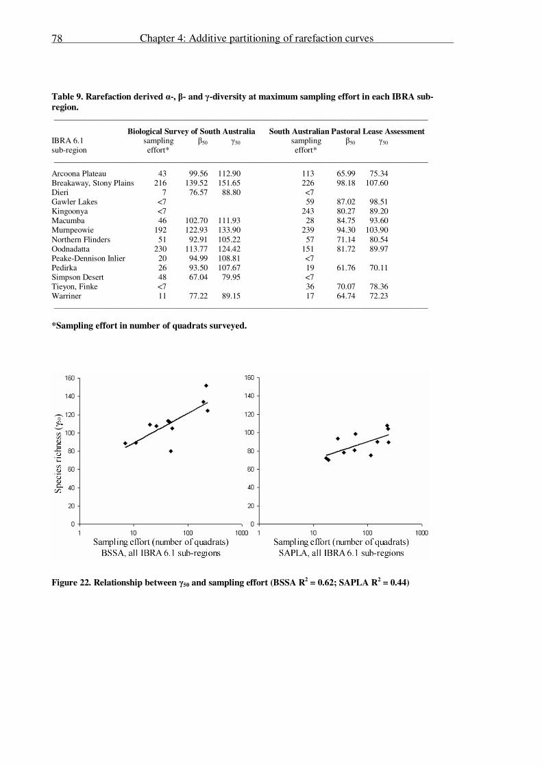
Chapter 4: Additive partitioning of rarefaction curves
78
Table 9. Rarefaction derived α-, β- and γ-diversity at maximum sampling effort in each IBRA sub-
region. __________________________________________________________________________________________
Biological Survey of South Australia South Australian Pastoral Lease Assessment IBRA 6.1 sampling β50 γ50 sampling β50 γ50 sub-region effort* effort* __________________________________________________________________________________________
Arcoona Plateau 43 99.56 112.90 113 65.99 75.34 Breakaway, Stony Plains 216 139.52 151.65 226 98.18 107.60 Dieri 7 76.57 88.80 <7 Gawler Lakes <7 59 87.02 98.51 Kingoonya <7 243 80.27 89.20 Macumba 46 102.70 111.93 28 84.75 93.60 Murnpeowie 192 122.93 133.90 239 94.30 103.90
Northern Flinders 51 92.91 105.22 57 71.14 80.54 Oodnadatta 230 113.77 124.42 151 81.72 89.97 Peake-Dennison Inlier 20 94.99 108.81 <7 Pedirka 26 93.50 107.67 19 61.76 70.11 Simpson Desert 48 67.04 79.95 <7 Tieyon, Finke <7 36 70.07 78.36 Warriner 11 77.22 89.15 17 64.74 72.23 __________________________________________________________________________________________
*Sampling effort in number of quadrats surveyed.
Figure 22. Relationship between γ50 and sampling effort (BSSA R2 = 0.62; SAPLA R
2 = 0.44)
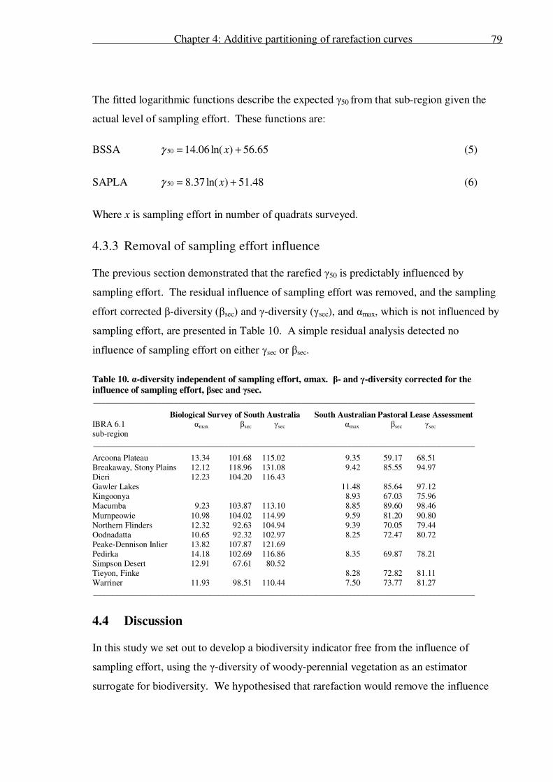
Chapter 4: Additive partitioning of rarefaction curves
79
The fitted logarithmic functions describe the expected γ50 from that sub-region given the
actual level of sampling effort. These functions are:
BSSA 65.56)ln(06.1450 += xγ (5)
SAPLA 48.51)ln(37.850 += xγ (6)
Where x is sampling effort in number of quadrats surveyed.
4.3.3 Removal of sampling effort influence
The previous section demonstrated that the rarefied γ50 is predictably influenced by
sampling effort. The residual influence of sampling effort was removed, and the sampling
effort corrected β-diversity (βsec) and γ-diversity (γsec), and αmax, which is not influenced by
sampling effort, are presented in Table 10. A simple residual analysis detected no
influence of sampling effort on either γsec or βsec.
Table 10. α-diversity independent of sampling effort, αmax. β- and γ-diversity corrected for the
influence of sampling effort, βsec and γsec. __________________________________________________________________________________________
Biological Survey of South Australia South Australian Pastoral Lease Assessment IBRA 6.1 αmax βsec γsec αmax βsec γsec sub-region __________________________________________________________________________________________
Arcoona Plateau 13.34 101.68 115.02 9.35 59.17 68.51 Breakaway, Stony Plains 12.12 118.96 131.08 9.42 85.55 94.97 Dieri 12.23 104.20 116.43 Gawler Lakes 11.48 85.64 97.12 Kingoonya 8.93 67.03 75.96 Macumba 9.23 103.87 113.10 8.85 89.60 98.46
Murnpeowie 10.98 104.02 114.99 9.59 81.20 90.80 Northern Flinders 12.32 92.63 104.94 9.39 70.05 79.44 Oodnadatta 10.65 92.32 102.97 8.25 72.47 80.72 Peake-Dennison Inlier 13.82 107.87 121.69 Pedirka 14.18 102.69 116.86 8.35 69.87 78.21 Simpson Desert 12.91 67.61 80.52 Tieyon, Finke 8.28 72.82 81.11 Warriner 11.93 98.51 110.44 7.50 73.77 81.27 __________________________________________________________________________________________
4.4 Discussion
In this study we set out to develop a biodiversity indicator free from the influence of
sampling effort, using the γ-diversity of woody-perennial vegetation as an estimator
surrogate for biodiversity. We hypothesised that rarefaction would remove the influence
Chapter 4: Additive partitioning of rarefaction curves
80
of sampling effort, and that additive partitioning would allow the extraction of γ-diversity
from the rarefaction curves.
Our analysis upheld our prediction that raw γ-diversity of each IBRA 6.1 sub-region would
be strongly influenced by sampling effort, and that raw α-diversity would not. Our
analysis also demonstrated that rarefaction did not remove the influence of sampling effort
on γ-diversity, thus disproving our hypothesis. However, we demonstrated that the
influence of sampling effort on γ-diversity was predictable, and therefore were able to
correct for this influence.
It is interesting to compare the final measures of α-, β- and γ-diversity extracted from the
BSSA and SAPLA. In all IBRA 6.1 sub-regions the BSSA records higher α-, β- and γ-
diversity species richness than the SAPLA, despite the larger quadrat size of the SAPLA
(Table 10). This was expected for two reasons, one methodological and one strategic.
Firstly, the BSSA and SAPLA employ different methodologies: BSSA surveys include a
botanical expert and SAPLA surveys do not. This difference alone could potentially
explain the higher species richness recorded by the BSSA. However, there is another
reason we expect the two surveys to record different species richness. The BSSA is an
inventory survey and is specifically designed to record as much of South Australia’s
species richness with as little sampling effort as possible. BSSA sites are systematically
located in less degraded areas of vegetation. In contrast, the SAPLA is designed to
monitor the effects of grazing by stock, and recording species richness is part of that
process, not its goal. The majority of SAPLA sites are located a moderate but regular
distance from stock watering points, and as such would be expected to exhibit some impact
of grazing pressure. We believe these two reasons adequately explain the difference in
species richness values recorded by our revised index for the two vegetation surveys.
The relationships we described between rarefied γ-diversity of woody-perennial vegetation
and sampling effort was derived empirically, and is specific to the study area, the taxon
studied, and the vegetation survey methods. Therefore, these relationships should not be
applied outside of our study area, to different taxa within our study area, or to data
collected by other vegetation surveys within our study area.
Chapter 4: Additive partitioning of rarefaction curves
81
An additional caveat is that our measure does not directly model and account for low
detectability plants. However, the methods presented herein should minimise the potential
impact of non-detection errors. By excluding ephemeral vegetation species, and limiting
the study to woody perennial vegetation species we removed a large source of potential for
non-detection errors. However, we have previously demonstrated significant non-
detection errors in the vegetation surveys used in this analysis (Chapter 3, Clarke et al.
submitted), even after limiting analysis to perennial species. By aggregating many sites in
a region, the rarefaction method used in our analyses should have further reduced the
influence of non-detection errors on γ-diversity: a low detectability species must only be
recorded at one site in a region to contribute to γ-diversity. However, non-detection errors
have probably artificially reduced α- and hence β-diversity in all sub-regions, although
these errors will be lower at higher sampling efforts.
Our research supports the findings by others that semi-log relationships describe
rarefaction curves well (Palmer 1990; Ugland et al. 2003). Additionally, our work answers
the call by Fleishman et al. (2006) to standardize measures of species richness for
differences in survey effort. However we have demonstrated that rarefaction alone does
not adequately control for the influence of sampling effort, a finding not previously
reported in the literature. If this relationship exists in other areas, interpolation or
extrapolation of rarefaction relationships without a sound understanding of the influence of
sampling effort will produce erroneous results.
These findings raise important questions for future research. Firstly, we need to ask
whether the relationship between rarefied β- and γ-diversity and sampling effort exists in
other areas. We have not sought a cause for the influence of sampling effort, but the
search for that cause is a logical next step. We consider it possible that the previously
mentioned non-detection errors are a partial cause of the relationship between rarefied
diversity and sampling effort. Heavily sampled regions not only detect more species due
to the expected influence of additional sampling on β- and γ-diversity, but also have more
opportunities to record species with low detectability than less sampled regions.
While the α-, β- and γ-diversity values reported in this paper are specific to the taxa
studied, vegetation quadrat survey methods and study area, the method we describe is
Chapter 4: Additive partitioning of rarefaction curves
82
transferable. The method outlined in this paper provides a theoretically sound framework
for deriving an indicator of α-, β- and γ-diversity which is comparable between regions of
different sampling effort. Our final sampling effort corrected measure of γ-diversity, γsec,
can conceivably be generated from any vegetation quadrat survey data obtained within a
prescribed methodology. Through the use of additive partitioning, γsec, is expressed in the
same units as, and directly comparable to, our sampling effort corrected measure of β-
diversity, βsec, and our sampling effort independent measure of α-diversity, αmax.
Application of our method will allow the extraction and comparison of α-, β- and γ-
diversity from previously under-utilised vegetation-quadrat survey data collected by
government agencies and non-government environmental organizations.
Lastly, we have argued that γ-diversity of woody-perennial vegetation is a theoretically
sound estimator-surrogate for biodiversity at broad scales. Therefore, by removing the
influence of sampling effort, our index allows examination of the real spatial variation of
biodiversity across the study area. However, due to the need to aggregate site data to
produce this index, the examination of variation in biodiversity is limited to a relatively
coarse spatial scale. The method presented here also facilitates examination of other
important components of biodiversity, namely the within sample (α), and between sample
(β) diversity.
4.5 Acknowledgements
This work was supported by funding from the Australian Desert Knowledge Cooperative
Research Centre (DKCRC) and the University of Adelaide. In addition, two DKCRC
partners provided the data that made this analysis possible, the South Australian
Department for Environment and Heritage and the South Australian Department of Water,
Land and Biodiversity Conservation. Finally, special thanks to Helen Vonow of the South
Australian State Herbarium for help in classifying and updating vegetation species lists.
Chapter 4: Additive partitioning of rarefaction curves
83
4.6 References
Badgley, C. and D. L. Fox (2000) Ecological biogeography of North America mammals: species density and ecological structure in relation to environmental gradients. Journal of Biogeography 27: 1437-1467. Boulinier, T., J. D. Nichols, J. R. Sauer, J. E. Hines and K. H. Pollock (1998) Estimating species richness: the importance of heterogeneity in species detectability. Ecology 79(3): 1018-1028.
Clarke, K. D., M. M. Lewis and B. Ostendorf (submitted) False negative errors in vegetation surveys. Biodiversity and Conservation?(?): ??-?? Colwell, R. K., C. X. Mao and J. Chang (2004) Interpolating, extrapolating, and comparing incidence-based species accumulation curves. Ecology 85(10): 2717-2727. Crist, T. O. and J. A. Veech (2006) Additive partitioning of rarefaction curves and species-area relationships: unifying alpha-, beta- and gamma-diversity with sample size and habitat area. Ecology Letters 9: 923-932.
Currie, D. J. and V. Paquin (1987) Large-scale biogeographical patterns of species richness of trees. Nature 329: 326-331. DWLBC (2002) Pastoral lease assessment, technical manual for assessing land condition on pastoral leases in South Australia, 1990–2000. Adelaide, Department of Water, Land and Biodiversity Conservation, Pastoral Program, Sustainable Resources. Fleishman, E., R. F. Noss and B. R. Noon (2006) Utility and limitations of species richness metrics for conservation
planning. Ecological Indicators 6(3): 543-553. Gotelli, N. J. and R. K. Colwell (2001) Quantifying biodiversity: procedures and pitfalls in the measurement and comparison of species richness. Ecology Letters 4(4): 379-391. Hawkins, B. A. and E. E. Porter (2003) Does herbivore diversity depend on plant diversity? The case of California butterflies. American Naturalist 161(1): 40-49.
Hawkins, B. A. and E. E. Porter (2003) Water-energy balance and the geographic pattern of species richness of western Palearctic butterflies. Ecological Entomology 28: 678-686. Hawkins, B. A., E. E. Porter and J. A. F. Diniz-Filho (2003) Productivity and history as predictors of the latitudinal diversity gradient of terrestrial birds. Ecology 84(6): 1608-1623. Heard, L. and B. Channon (1997) Guide to a native vegetation survey: Using the Biological Survey of South Australia. Adelaide, SA, Department of Environment and Natural Resources.
Laut, P., G. Keig, M. Lazarides, E. Loffler, C. Margules, R. M. Scott and M. E. Sullivan (1977) Environments of South Australia: Province 8, Northern Arid. Canberra, Division of Land Use Research, CSIRO: 116-168. Mao, C. X., R. K. Colwell and J. Chang (2005) Estimating the species accumulation curve using mixtures. Biometrics 61: 433-441. O'Brien, E. M. (1993) Climatic gradients in woody plant species richness: towards an explanation based on an analysis of
Southern Africa's woody flora. Journal of Biogeography 20: 181-198. O'Brien, E. M. (1998) Water-energy dynamics, climate, and prediction of woody plants species richness: an interim general model. Journal of Biogeography 25: 379-398. O'Brien, E. M., R. Field and R. J. Whittaker (2000) Climatic gradients in woody plant (tree and shrub) diversity: water-energy dynamics, residual variation, and topography. Oikos 89(3): 588-600. Palmer, M. W. (1990) The estimation of species richness by extrapolation. Ecology 71(3): 1195-1198.
Rodrigues, A. S. L. and T. M. Brooks (2007) Shortcuts for biodiversity conservation planning: the effectiveness of surrogates. Annual Review of Ecology, Evolution, and Systematics 38(1): 713-737. Sarkar, S. (2002) Defining "Biodiversity"; Assessing Biodiversity. The Monist 85(1): 131-155.

Chapter 4: Additive partitioning of rarefaction curves
84
Smyth, A. K., V. H. Chewings, G. N. Bastin, S. Ferrier, G. Manion and B. Clifford (2004) Integrating historical datasets to prioritise areas for biodiversity monitoring? Australian Rangelands Society 13th Biennial Conference: "Living in the
outback", Alice Springs, Northern Territory. Tipper, J. C. (1979) Rarefaction and Rarefiction-The Use and Abuse of a Method in Paleoecology. Paleobiology 5(4): 423-434. Ugland, K. I., J. S. Gray and K. E. Ellingsen (2003) The species-accumulation curve and estimation of species richness. Journal of Animal Ecology 72: 888-897.
Veech, J. A., K. S. Summerville, T. O. Crist and J. C. Gering (2002) The additive partitioning of species diversity: recent revival of an old idea. Oikos 99: 3-9. Venevsky, S. and I. Venevskaia (2005) Heirarchical systematic conservation planning at the national level: Identifying national biodiversity hotspots using abiotic factors in Russia. Biological Conservation 124: 235-251. Whittaker, R. H. (1972) Evolution and measurement of species diversity. Taxon 21(2/3): 213-251.
Chapter 5: Remotely sensed surrogates of biodiversity stress
85
Chapter 5: Remotely sensed surrogates of biodiversity stress
5.1 Introduction
As we become more environmentally aware, and as economic values are placed on natural
ecosystems (Costanza et al. 1997), managers have begun to appreciate the potential cost of
allowing further degradation of our natural systems. In the Australian rangelands this has
resulted in an increased desire to monitor and manage biodiversity for conservation (Smyth
et al. 2004). But how can we best measure biodiversity?
The term biodiversity is so all-encompassing that direct measurement is not possible, and it
is necessary to measure other features which vary with biodiversity: surrogates. Sarkar
(2002) argued that species richness was one of the few suitable true-surrogates for
biodiversity because firstly, species are a well defined and understood category, and
secondly, species richness is measurable. However measuring total species richness at any
reasonable scale is not feasible. We have previously argued that woody perennial
vegetation γ-diversity is a surrogate for total species richness, and hence a suitable
estimator-surrogate for biodiversity (Clarke et al. submitted).
A surrogate which is practically measurable at broad scales must be established for total
species richness, as an indicator-surrogate for biodiversity (Sarkar 2002). To do this we
need to understand, at broad scales, the causes of and pressures on biodiversity in the arid
and semi-arid rangelands of South Australia.
We have previously argued that the most compelling explanation for the distribution of
biodiversity at broad scales is the “species-energy hypothesis,” and the most significant
pressure on biodiversity in the study area is grazing-induced degradation, or overgrazing
(Chapter 2). In examining the causes of and pressures on biodiversity, we see two
potential surrogates of pressure on biodiversity which may be practical at broad scales.
The first surrogate we propose is based on the differential effect of overgrazing on water-
energy balance and net primary productivity. Firstly, water-energy balance is a function of
climatic variables and the redistribution of rainfall by topography, and therefore
Chapter 5: Remotely sensed surrogates of biodiversity stress
86
independent of grazing disturbance. Therefore we will treat water-energy balance as an
index of potential, or expected primary productivity. Conversely, net primary productivity
is reduced by high grazing pressure. Given the differential influence of disturbance, we
hypothesise that the difference between expected and net primary production will provide a
measure of biodiversity-reducing disturbance in the study area.
The second surrogate we propose is based on the convincing link between grazing induced
degradation and the temporal variability of net primary productivity and rainfall use
efficiency. We propose the measurement of average and variation in annual net primary
productivity and rainfall use efficiency as a tool for monitoring grazing induced landscape
degradation, and hence pressure on biodiversity.
In this study a measurement of net primary productivity is derived from satellite imagery,
water-energy balance is derived from climatic data, and rainfall use efficiency is derived
from the combination of satellite imagery and climatic data. The two surrogates of
pressure on biodiversity are examined in relation to our index of woody perennial
vegetation α-, β- and γ-diversity derived from conventional vegetation quadrat surveys
(Chapter 4, or Clarke et al. submitted). We have previously argued that woody perennial
vegetation γ-diversity is a surrogate for total species richness, and hence a suitable
estimator-surrogate for biodiversity (Clarke et al. submitted). For this validation we are
assuming that prolonged biodiversity stress will result in low α-, β- and γ-diversity, and
hence that high values of our biodiversity-stress index will coincide with low α-, β- and γ-
diversity, and vice versa.
5.2 Methods
5.2.1 Study area
A more detailed description of the study area can be found in Chapter 1. The surrogates of
biodiversity stress were developed in, and are restricted to the study area. Woody
perennial alpha, beta and gamma diversity derived from the Biological Survey of South
Australia data (Chapter 4, or Clarke et al. submitted) is presented in Figure 23.
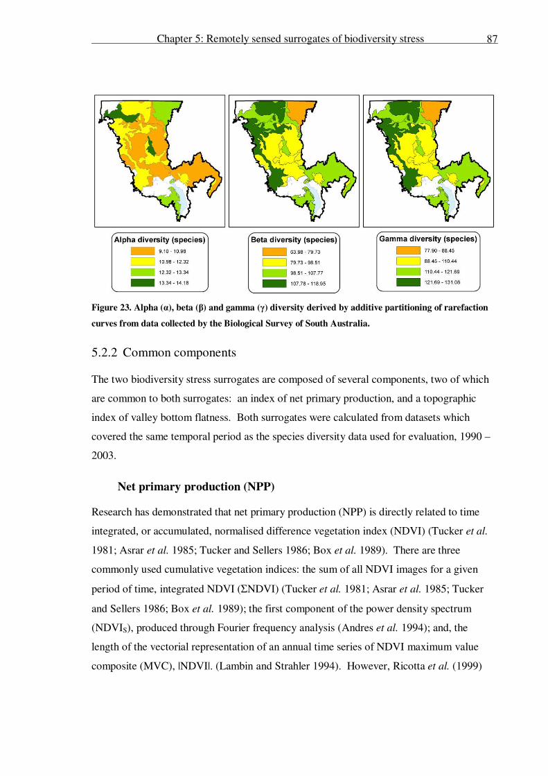
Chapter 5: Remotely sensed surrogates of biodiversity stress
87
Figure 23. Alpha (α), beta (β) and gamma (γ) diversity derived by additive partitioning of rarefaction
curves from data collected by the Biological Survey of South Australia.
5.2.2 Common components
The two biodiversity stress surrogates are composed of several components, two of which
are common to both surrogates: an index of net primary production, and a topographic
index of valley bottom flatness. Both surrogates were calculated from datasets which
covered the same temporal period as the species diversity data used for evaluation, 1990 –
2003.
Net primary production (NPP)
Research has demonstrated that net primary production (NPP) is directly related to time
integrated, or accumulated, normalised difference vegetation index (NDVI) (Tucker et al.
1981; Asrar et al. 1985; Tucker and Sellers 1986; Box et al. 1989). There are three
commonly used cumulative vegetation indices: the sum of all NDVI images for a given
period of time, integrated NDVI (ΣNDVI) (Tucker et al. 1981; Asrar et al. 1985; Tucker
and Sellers 1986; Box et al. 1989); the first component of the power density spectrum
(NDVIS), produced through Fourier frequency analysis (Andres et al. 1994); and, the
length of the vectorial representation of an annual time series of NDVI maximum value
composite (MVC), |NDVI|. (Lambin and Strahler 1994). However, Ricotta et al. (1999)
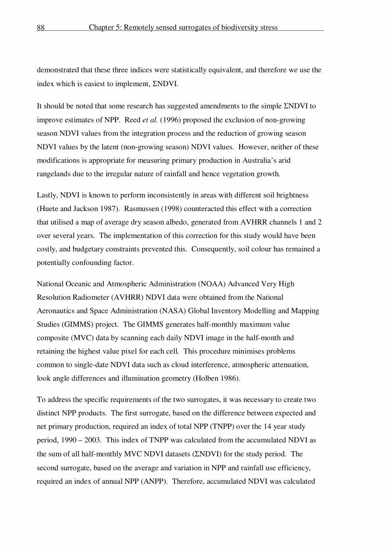
Chapter 5: Remotely sensed surrogates of biodiversity stress
88
demonstrated that these three indices were statistically equivalent, and therefore we use the
index which is easiest to implement, ΣNDVI.
It should be noted that some research has suggested amendments to the simple ΣNDVI to
improve estimates of NPP. Reed et al. (1996) proposed the exclusion of non-growing
season NDVI values from the integration process and the reduction of growing season
NDVI values by the latent (non-growing season) NDVI values. However, neither of these
modifications is appropriate for measuring primary production in Australia’s arid
rangelands due to the irregular nature of rainfall and hence vegetation growth.
Lastly, NDVI is known to perform inconsistently in areas with different soil brightness
(Huete and Jackson 1987). Rasmussen (1998) counteracted this effect with a correction
that utilised a map of average dry season albedo, generated from AVHRR channels 1 and 2
over several years. The implementation of this correction for this study would have been
costly, and budgetary constraints prevented this. Consequently, soil colour has remained a
potentially confounding factor.
National Oceanic and Atmospheric Administration (NOAA) Advanced Very High
Resolution Radiometer (AVHRR) NDVI data were obtained from the National
Aeronautics and Space Administration (NASA) Global Inventory Modelling and Mapping
Studies (GIMMS) project. The GIMMS generates half-monthly maximum value
composite (MVC) data by scanning each daily NDVI image in the half-month and
retaining the highest value pixel for each cell. This procedure minimises problems
common to single-date NDVI data such as cloud interference, atmospheric attenuation,
look angle differences and illumination geometry (Holben 1986).
To address the specific requirements of the two surrogates, it was necessary to create two
distinct NPP products. The first surrogate, based on the difference between expected and
net primary production, required an index of total NPP (TNPP) over the 14 year study
period, 1990 – 2003. This index of TNPP was calculated from the accumulated NDVI as
the sum of all half-monthly MVC NDVI datasets (ΣNDVI) for the study period. The
second surrogate, based on the average and variation in NPP and rainfall use efficiency,
required an index of annual NPP (ANPP). Therefore, accumulated NDVI was calculated
Chapter 5: Remotely sensed surrogates of biodiversity stress
89
for each of the 14 study years, 1990 – 2003, as the sum of all half-monthly MVC NDVI
datasets (ΣNDVI) for that year
Topographic index: valley bottom flatness (VBF)
Both surrogates required a method for accounting for the redistribution of rainfall by
terrain. To this end a topographic index titled multiple resolution valley bottom flatness
(VBF) was calculated (Gallant and Dowling 2003). The VBF index classifies the
landscape into valley bottom and non-valley bottom (slope and ridge) areas, which in the
context of rainfall redistribution correspond to run-on and run-off areas respectively.
Chapter 5: Remotely sensed surrogates of biodiversity stress
90
Figure 24. Elevation in the study area as recorded by the AUSLIG 9 second (~310 m) digital elevation
model (DEM). IBRA 6.1 sub-region boundaries are overlain for interpretation; see Figure 25 for
IBRA sub-region detail.
The VBF index was calculated from the AUSLIG 9 second (approximately 310 m) digital
elevation model (DEM) (Figure 24). Due to software requirements, the DEM was
resampled to 325 m prior to generation of the VBF index. The specific use of the VBF in
each surrogate is discussed in the relevant sub-section: Surrogate 1, Evapotranspiration
and topographic redistribution of rainfall; and Surrogate 2, Topographically redistributed
rainfall.
5.2.3 Surrogate 1
In addition to the index of TNPP, Surrogate 1 requires one specific component, a measure
of expected primary production derived from climatic data, actual evapotranspiration. The
generation of this component is discussed below, followed by the details of the calculation
of Surrogate 1 from the components.
Expected primary production (EPP)
Studies of water-energy balance in relation to variation in biodiversity have used several
different measures of water-energy balance. One of the most widely used is actual
evapotranspiration, a measure of the availability of water for transpiration in relation to
ambient energy conditions (Currie and Paquin 1987; Currie 1991; O'Brien 1993; O'Brien
1998; Badgley and Fox 2000; Hawkins and Porter 2003; Hawkins and Porter 2003;
Hawkins et al. 2003).
Actual evapotranspiration (hereafter AET) data were obtained from the Australian Bureau
of Meteorology collaborative SILO project (Jeffrey et al. 2001). The SILO project
employs Morton’s complementary relationship areal evapotranspiration (CRAE) model
(Morton 1983), a model which has performed well in extensive tests across different
climatic regions (Hobbins et al. 2001). The SILO project calculates AET from climatic
variables recorded at discrete climate stations, and a raster surface is then interpolated to
create an Australia-wide AET surface with a resolution of 5 km.
Specifically, average monthly AET was obtained for the study period, 1990 to 2003.
However, the capacity for species richness is determined by the amount, and duration of

Chapter 5: Remotely sensed surrogates of biodiversity stress
91
biological activity (O'Brien 2006). Therefore, the AET data were transformed to total
accumulated AET, or AAET. This was accomplished by multiplying each month’s
average AET by the number of days in the month to produce monthly total, or
accumulated, AET, in mm evapotranspiration. Within each year, monthly accumulated
AET data were summed to produce yearly AET. Finally, yearly AET was summed to
produce accumulated AET (AAET) for the 14 year study period, a theoretical index of
expected primary production (EPP).
Topographically scaled EPP (TEPP)
Rainfall is a significant component of AET, but the SILO rainfall data are relatively coarse
scale (see sub-section 0, Rainfall, for more detail). To account for the redistribution of
rainfall by topography, the VBF index was scaled and combined with the AAET raster.
This was done in such a way that evapotranspiration values on steep slopes remained
unchanged, while values in valley bottoms were increased by up to 100%. Specifically,
VBF was scaled from 1 – 2 and multiplied by AAET. This produced a topographically
scaled index of expected primary production (TEPP). Finally, to facilitate comparison this
index with the satellite derived index of actual primary production the TEPP was rescaled
to 8 km resolution.
Calculation of Surrogate 1
The index of biodiversity-stress, Surrogate 1, was calculated as:
)/(1 TEPPTNPP− (1)
Where TNPP is an index of total NPP over the 14 year study period and TEPP is an index
of topographically scaled index of expected primary production. This method of
calculation produced an intuitive index where low values of biodiversity-stress index
would indicate that actual primary production is close to its climatic potential; and high
values of biodiversity-stress index would indicate that actual primary production is falling
short of climatic potential.
Chapter 5: Remotely sensed surrogates of biodiversity stress
92
5.2.4 Surrogate 2
In addition to ANPP, Surrogate 2 requires an index of rainfall use efficiency (RUE). The
calculation of RUE from rainfall and NPP data are discussed below, followed by the
method used to calculate Surrogate 2.
Rainfall
There are 22 climate stations which measure rainfall within the study area. However, the
rainfall surface is interpolated from all climate stations within 100 km, with a minimum
requirement of 30 climate stations. If there are fewer than 30 climate stations within 100
km the radius is increased iteratively until this criterion is satisfied (Jeffrey et al. 2001).
Due to the low density of climate stations in and around the study area, rainfall at any
given point is interpolated from data collected at stations ranging from a few kilometres to
several hundred kilometres away. Thus, the data supplied by the Australian Bureau of
Meteorology collaborative SILO project (Jeffrey et al. 2001) makes no allowance for
orographic influences on rainfall (uplift or rain-shadowing), or for the topographic re-
distribution of rain by slopes (run-off areas) and valley flats and rivers (run-on areas).
Two rainfall indices were used in the analyses; climatically distributed rainfall as depicted
by the SILO interpolation, and topographically re-distributed rainfall.
Climatically distributed rainfall use efficiency (CRUE)
The data obtained from the Australian Bureau of Meteorology collaborative SILO project
(Jeffrey et al. 2001) makes no allowance for factors which cause meso-scale variation in
rainfall, and is therefore treated as a measure of climatically distributed rainfall. Average
monthly rainfall was obtained for the study period, 1990 to 2003 at 5 km resolution. From
the average monthly rainfall, total annual rainfall (AR) was calculated for each of the 14
study years. Finally, the AR was resampled to 8 km resolution to facilitate comparison
with the satellite derived index of net primary production (also at 8 km resolution).
Climatically distributed rainfall use efficiency (CRUE) was calculated for each of the 14
study years by dividing NPP for that year by the AR for the same 12 month period. This
method is analogous to the method used by Holm et al. (2003), where RUE was calculated
as total phytomass per mm of rainfall in the preceding 12 months.
Chapter 5: Remotely sensed surrogates of biodiversity stress
93
Topographically redistributed rainfall use efficiency (TRUE)
To account for the redistribution of rainfall by topography, the VBF index was scaled and
combined with the total annual rainfall rasters to produce a topographically scaled annual
rainfall index (T-AR) for each of the 14 study years. The was done in such a way that
rainfall values on steep slopes remained unchanged, while values in valley bottoms were
increased by up to 100%. Specifically, VBF was scaled from 1 – 2 and multiplied by AR.
Finally, the T-AR was resampled to 8 km resolution to facilitate comparison with the
satellite derived index of net primary production (also at 8 km resolution).
Topographically redistributed rainfall use efficiency (TRUE) was very similar to the
calculation of CRUE, with T-AR taking the place of AR.
Calculation of Surrogate 2
The average annual, and annual variation (standard deviation) were calculated for NPP,
CRUE and TRUE. These were calculated as the average and standard deviation at each 8
km pixel location over the 14 annual RUE datasets. This resulted in six outputs, mean
annual NPP (mean-NPP), annual variation in NPP (std-NPP), mean annual CRUE (mean-
CRUE), annual variation in CRUE (std-CRUE), mean annual TRUE (mean-TRUE) and
annual variation in TRUE (std-TRUE).
5.2.5 Evaluation method
High biodiversity-stress is expected to cause a reduction in woody perennial vegetation α-,
β- and γ-diversity. Therefore, both surrogates of biodiversity-stress were compared to our
measure of woody perennial vegetation α-, β- and γ-diversity values extracted from
vegetation quadrat data collected by two surveys: the Biological Survey of South Australia
(BSSA); and the South Australian Pastoral Lease Assessment (Chapter 4, or Clarke et al.
submitted).
However, the α-, β- and γ-diversity values were generated from quadrat surveys at point
locations and then aggregated by IBRA sub-region, while the biodiversity-stress index is a
continuous surface. To ensure similar areas were compared, the value of the
corresponding biodiversity-stress index pixel (8 km resolution) was extracted for each
vegetation survey quadrat location and then averaged by IBRA sub-region (Figure 25).

Chapter 5: Remotely sensed surrogates of biodiversity stress
94
Thus, α-, β- and γ-diversity value, and average surrogate values were calculated for each
IBRA sub-region. Finally, correlation was examined between each type of diversity from
both conventional vegetation surveys and all surrogates of biodiversity stress.
Figure 25. IBRA 6.1 sub-region name, location and extent.
5.3 Results
5.3.1 Common component: index of valley bottom flatness (VBF)
The topographic index, multiple resolution valley bottom flatness (VBF) is presented in
Figure 26. Inspection of the VBF index in relation to the parent digital elevation model

Chapter 5: Remotely sensed surrogates of biodiversity stress
95
(Figure 24) showed reasonably good agreement. The extensive flat areas in the north east
and other parts of the study area correspond to dune filed and known valley bottoms, and
the steep areas correspond to known ranges and other regions of high relief. However, the
index sometimes struggled to distinguish ridge tops from valley bottoms, and in flat terrain
sometimes failed to map valley bottoms.
Figure 26. Multiple resolution valley bottom flatness (VBF) index, calculated from the AUSLIG 9
second digital elevation model (DEM). Resolution is 325 m.
Chapter 5: Remotely sensed surrogates of biodiversity stress
96
5.3.2 Surrogate 1
Total net primary production (TNPP)
The index of net primary production used in Surrogate 1, total net primary production
(TNPP), is presented in Figure 27. Two interesting features become apparent by comparing
TNPP to IBRA sub-region boundaries (Figure 25); the tongue of high primary production
in the north-west of the study area corresponds very closely to the Pedirka and Tieyon,
Finke sub-regions. Additionally, a line of high TNPP is visible around about 28° S,
following the edge of the Breakaways, Stony Plains and Oodnadatta sub-regions. These
patches of high TNPP could either be the result of true variation in the spatial distribution
of primary production as a result of soil type, rainfall and topography, or an error caused
by the known influence of soil colour on NDVI.
Inspection of high-resolution QuickBird imagery (not shown) shows substantially greater
vegetation cover in the Pedirka and Tieyon, Finke sub-regions than in surrounding areas.
Likewise, two large tree-lined ephemeral rivers flow through the Oodnadatta and Peake-
Dennison Inlier sub-region along 28° S, the Arckaringa Creek and the Neales
(Nappamurra) River. Thus, this mapped variation in primary production corresponds to
the on-ground variation in primary production, and not to artefacts related to soil colour.
Expected primary production (EPP)
The surrogate for expected primary production (EPP), accumulated Morton’s actual
evapotranspiration (AAET) is presented in Figure 28. The map has two main features of
interest. Firstly, there is a pronounced gradient of EPP, ranging from low in the north to
high in the south. Secondly, the map displays no local or regional deviation from this even
gradient.
AAET, and hence EPP in the study area is primarily driven by rainfall; energy is not
limiting in arid Australia. The direction of the gradient is a result of the location of the
study area in relation to Australia’s coast; less rain falls further inland. The southern end
of the study area is relatively close to the Australian coast, specifically Spencer Gulf,
receives more rainfall and has a higher EPP; the northern end of the study area is further
away from the coast, receives less rainfall and has a lower EPP; the north-eastern corner of
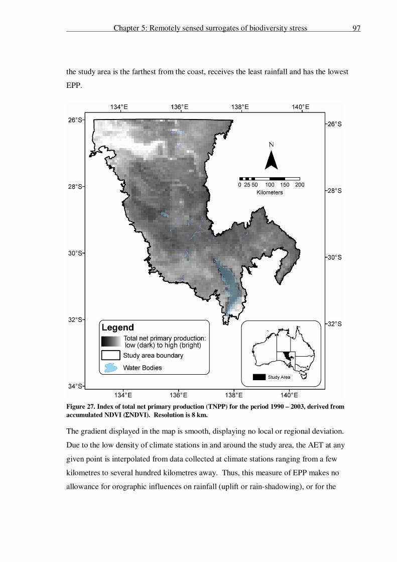
Chapter 5: Remotely sensed surrogates of biodiversity stress
97
the study area is the farthest from the coast, receives the least rainfall and has the lowest
EPP.
Figure 27. Index of total net primary production (TNPP) for the period 1990 – 2003, derived from
accumulated NDVI (ΣΣΣΣNDVI). Resolution is 8 km.
The gradient displayed in the map is smooth, displaying no local or regional deviation.
Due to the low density of climate stations in and around the study area, the AET at any
given point is interpolated from data collected at climate stations ranging from a few
kilometres to several hundred kilometres away. Thus, this measure of EPP makes no
allowance for orographic influences on rainfall (uplift or rain-shadowing), or for the
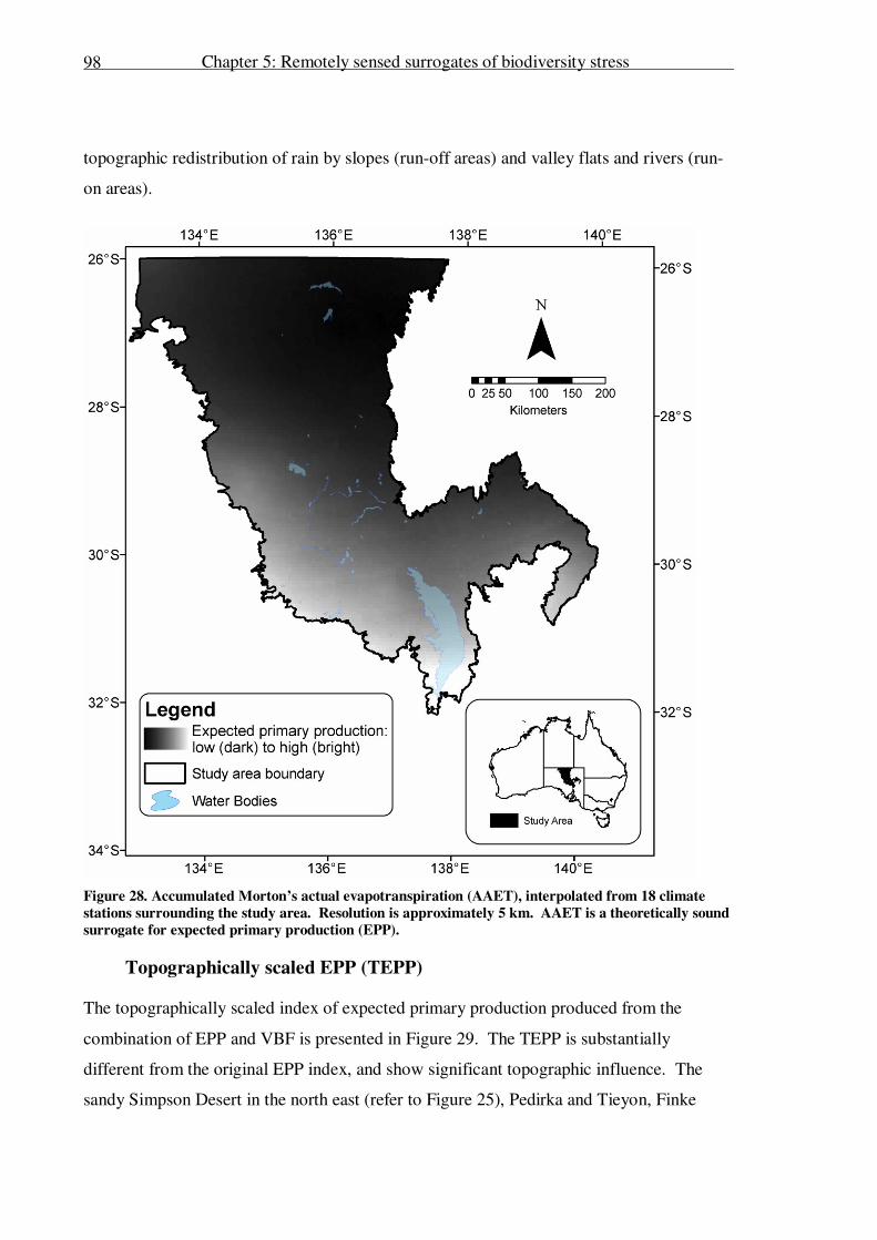
Chapter 5: Remotely sensed surrogates of biodiversity stress
98
topographic redistribution of rain by slopes (run-off areas) and valley flats and rivers (run-
on areas).
Figure 28. Accumulated Morton’s actual evapotranspiration (AAET), interpolated from 18 climate
stations surrounding the study area. Resolution is approximately 5 km. AAET is a theoretically sound
surrogate for expected primary production (EPP).
Topographically scaled EPP (TEPP)
The topographically scaled index of expected primary production produced from the
combination of EPP and VBF is presented in Figure 29. The TEPP is substantially
different from the original EPP index, and show significant topographic influence. The
sandy Simpson Desert in the north east (refer to Figure 25), Pedirka and Tieyon, Finke
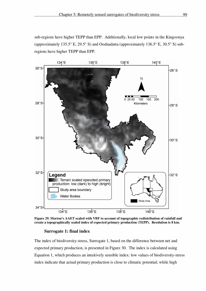
Chapter 5: Remotely sensed surrogates of biodiversity stress
99
sub-regions have higher TEPP than EPP. Additionally, local low points in the Kingoonya
(approximately 135.5° E, 29.5° S) and Oodnadatta (approximately 136.5° E, 30.5° S) sub-
regions have higher TEPP than EPP.
Figure 29. Morton’s AAET scaled with VBF to account of topographic redistribution of rainfall and
create a topographically scaled index of expected primary production (TEPP). Resolution is 8 km.
Surrogate 1: final index
The index of biodiversity-stress, Surrogate 1, based on the difference between net and
expected primary production, is presented in Figure 30. The index is calculated using
Equation 1, which produces an intuitively sensible index: low values of biodiversity-stress
index indicate that actual primary production is close to climatic potential; while high
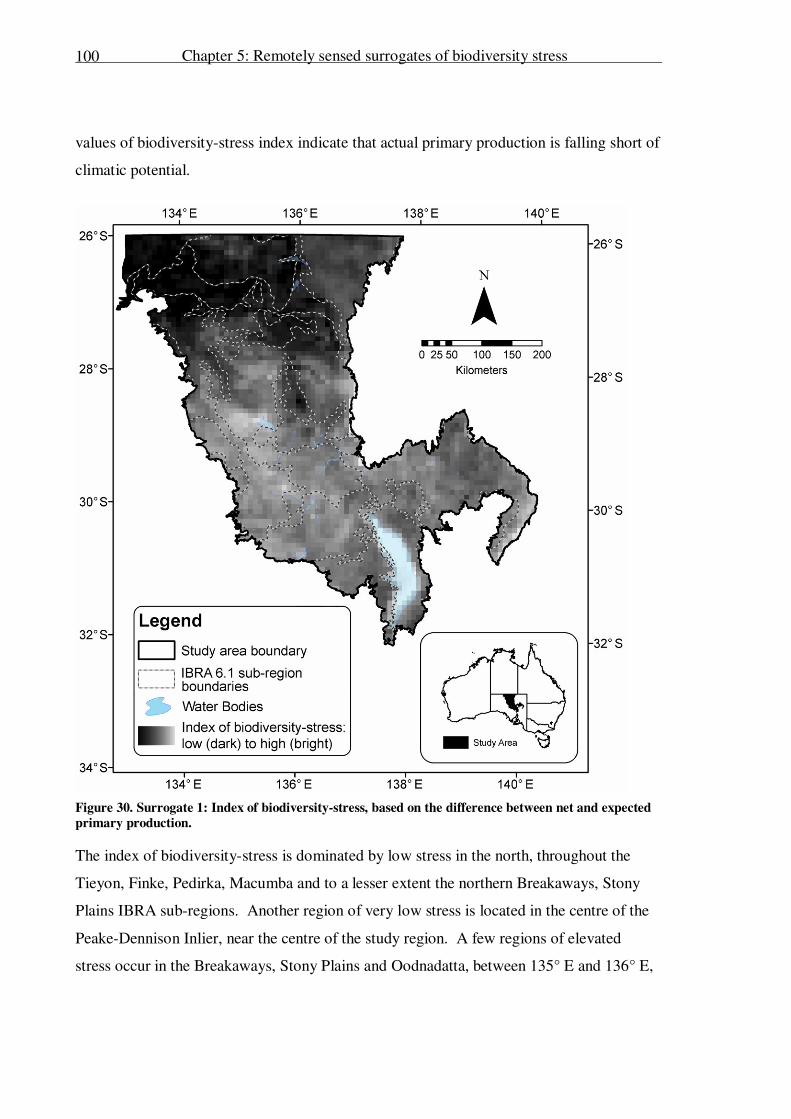
Chapter 5: Remotely sensed surrogates of biodiversity stress
100
values of biodiversity-stress index indicate that actual primary production is falling short of
climatic potential.
Figure 30. Surrogate 1: Index of biodiversity-stress, based on the difference between net and expected
primary production.
The index of biodiversity-stress is dominated by low stress in the north, throughout the
Tieyon, Finke, Pedirka, Macumba and to a lesser extent the northern Breakaways, Stony
Plains IBRA sub-regions. Another region of very low stress is located in the centre of the
Peake-Dennison Inlier, near the centre of the study region. A few regions of elevated
stress occur in the Breakaways, Stony Plains and Oodnadatta, between 135° E and 136° E,
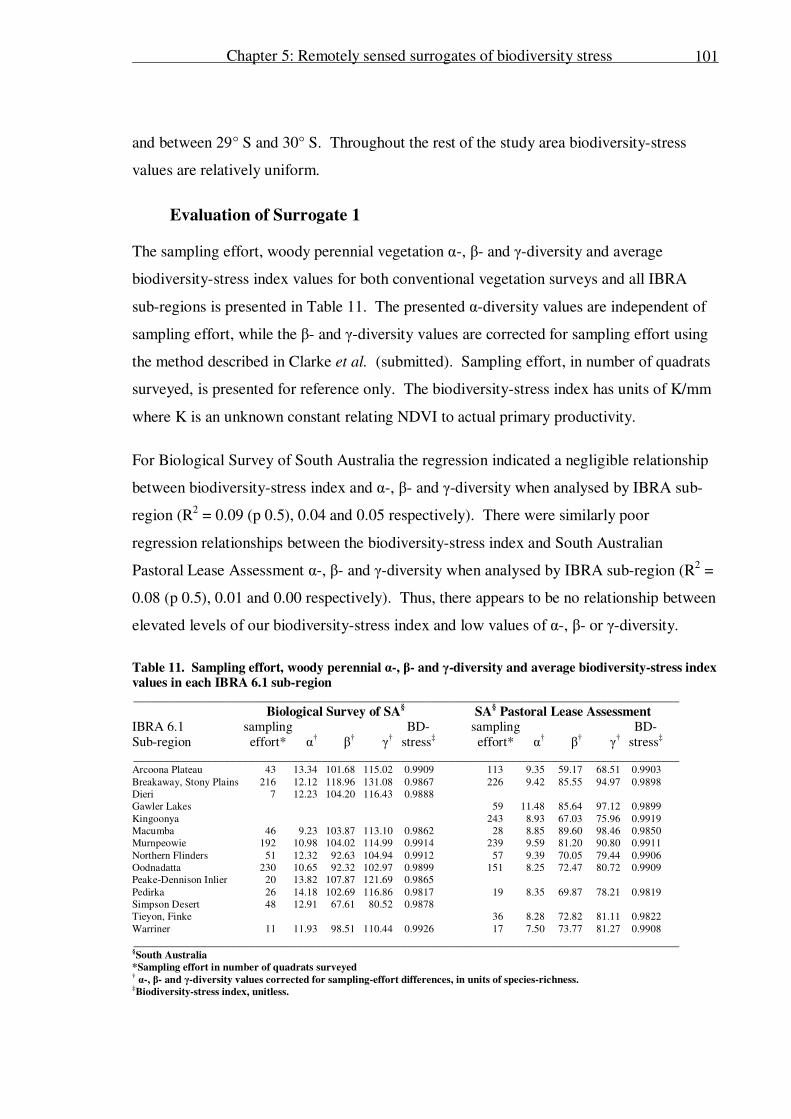
Chapter 5: Remotely sensed surrogates of biodiversity stress
101
and between 29° S and 30° S. Throughout the rest of the study area biodiversity-stress
values are relatively uniform.
Evaluation of Surrogate 1
The sampling effort, woody perennial vegetation α-, β- and γ-diversity and average
biodiversity-stress index values for both conventional vegetation surveys and all IBRA
sub-regions is presented in Table 11. The presented α-diversity values are independent of
sampling effort, while the β- and γ-diversity values are corrected for sampling effort using
the method described in Clarke et al. (submitted). Sampling effort, in number of quadrats
surveyed, is presented for reference only. The biodiversity-stress index has units of K/mm
where K is an unknown constant relating NDVI to actual primary productivity.
For Biological Survey of South Australia the regression indicated a negligible relationship
between biodiversity-stress index and α-, β- and γ-diversity when analysed by IBRA sub-
region (R2 = 0.09 (p 0.5), 0.04 and 0.05 respectively). There were similarly poor
regression relationships between the biodiversity-stress index and South Australian
Pastoral Lease Assessment α-, β- and γ-diversity when analysed by IBRA sub-region (R2 =
0.08 (p 0.5), 0.01 and 0.00 respectively). Thus, there appears to be no relationship between
elevated levels of our biodiversity-stress index and low values of α-, β- or γ-diversity.
Table 11. Sampling effort, woody perennial α-, β- and γ-diversity and average biodiversity-stress index values in each IBRA 6.1 sub-region __________________________________________________________________________________________
Biological Survey of SA§ SA
§ Pastoral Lease Assessment
IBRA 6.1 sampling BD- sampling BD-
Sub-region effort* α† β† γ† stress‡ effort* α† β† γ† stress‡
__________________________________________________________________________________________ Arcoona Plateau 43 13.34 101.68 115.02 0.9909 113 9.35 59.17 68.51 0.9903
Breakaway, Stony Plains 216 12.12 118.96 131.08 0.9867 226 9.42 85.55 94.97 0.9898
Dieri 7 12.23 104.20 116.43 0.9888
Gawler Lakes 59 11.48 85.64 97.12 0.9899
Kingoonya 243 8.93 67.03 75.96 0.9919
Macumba 46 9.23 103.87 113.10 0.9862 28 8.85 89.60 98.46 0.9850
Murnpeowie 192 10.98 104.02 114.99 0.9914 239 9.59 81.20 90.80 0.9911
Northern Flinders 51 12.32 92.63 104.94 0.9912 57 9.39 70.05 79.44 0.9906
Oodnadatta 230 10.65 92.32 102.97 0.9899 151 8.25 72.47 80.72 0.9909
Peake-Dennison Inlier 20 13.82 107.87 121.69 0.9865
Pedirka 26 14.18 102.69 116.86 0.9817 19 8.35 69.87 78.21 0.9819
Simpson Desert 48 12.91 67.61 80.52 0.9878
Tieyon, Finke 36 8.28 72.82 81.11 0.9822
Warriner 11 11.93 98.51 110.44 0.9926 17 7.50 73.77 81.27 0.9908
__________________________________________________________________________________________ §South Australia
*Sampling effort in number of quadrats surveyed † α-, β- and γ-diversity values corrected for sampling-effort differences, in units of species-richness.
‡Biodiversity-stress index, unitless.
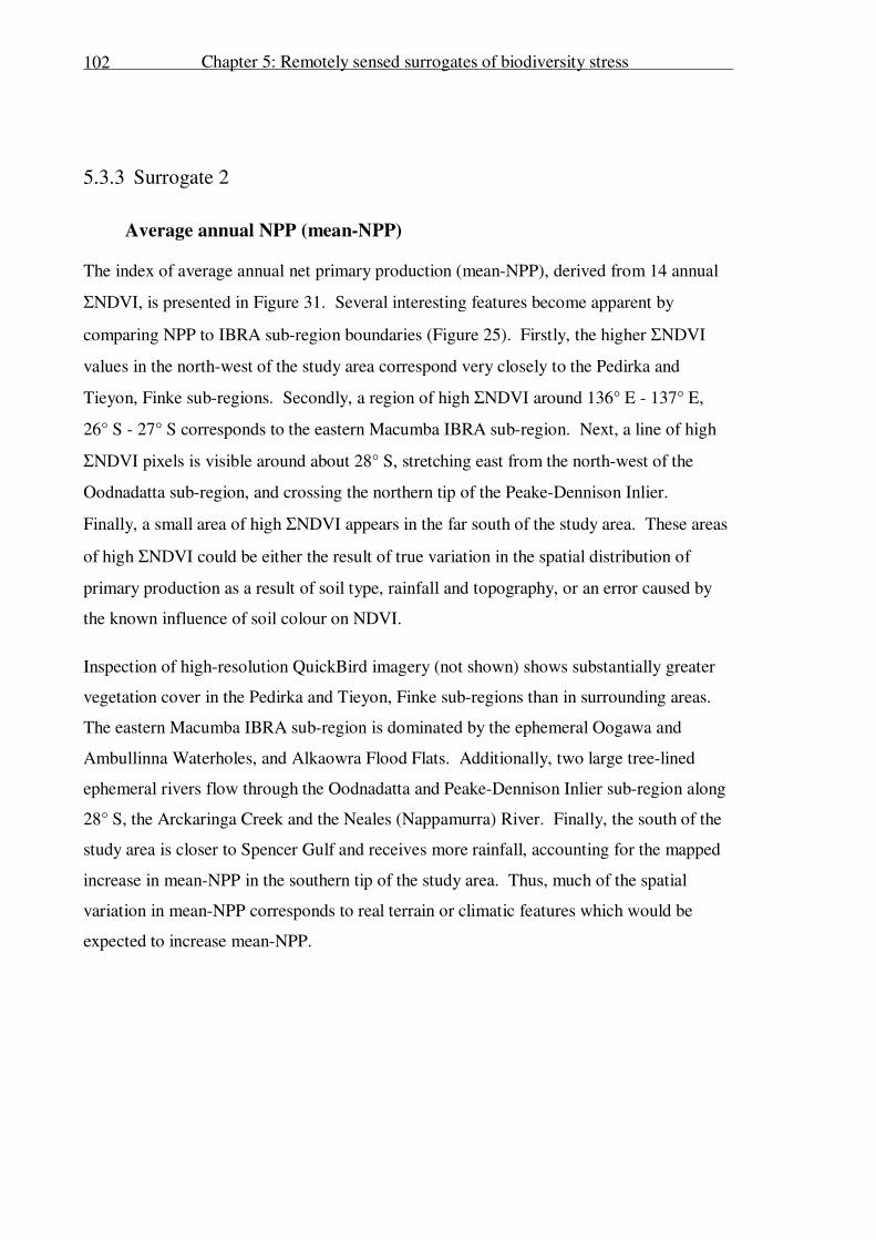
Chapter 5: Remotely sensed surrogates of biodiversity stress
102
5.3.3 Surrogate 2
Average annual NPP (mean-NPP)
The index of average annual net primary production (mean-NPP), derived from 14 annual
ΣNDVI, is presented in Figure 31. Several interesting features become apparent by
comparing NPP to IBRA sub-region boundaries (Figure 25). Firstly, the higher ΣNDVI
values in the north-west of the study area correspond very closely to the Pedirka and
Tieyon, Finke sub-regions. Secondly, a region of high ΣNDVI around 136° E - 137° E,
26° S - 27° S corresponds to the eastern Macumba IBRA sub-region. Next, a line of high
ΣNDVI pixels is visible around about 28° S, stretching east from the north-west of the
Oodnadatta sub-region, and crossing the northern tip of the Peake-Dennison Inlier.
Finally, a small area of high ΣNDVI appears in the far south of the study area. These areas
of high ΣNDVI could be either the result of true variation in the spatial distribution of
primary production as a result of soil type, rainfall and topography, or an error caused by
the known influence of soil colour on NDVI.
Inspection of high-resolution QuickBird imagery (not shown) shows substantially greater
vegetation cover in the Pedirka and Tieyon, Finke sub-regions than in surrounding areas.
The eastern Macumba IBRA sub-region is dominated by the ephemeral Oogawa and
Ambullinna Waterholes, and Alkaowra Flood Flats. Additionally, two large tree-lined
ephemeral rivers flow through the Oodnadatta and Peake-Dennison Inlier sub-region along
28° S, the Arckaringa Creek and the Neales (Nappamurra) River. Finally, the south of the
study area is closer to Spencer Gulf and receives more rainfall, accounting for the mapped
increase in mean-NPP in the southern tip of the study area. Thus, much of the spatial
variation in mean-NPP corresponds to real terrain or climatic features which would be
expected to increase mean-NPP.
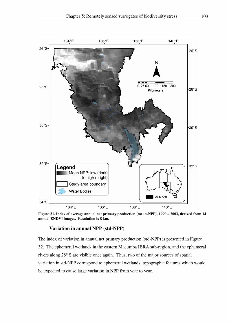
Chapter 5: Remotely sensed surrogates of biodiversity stress
103
Figure 31. Index of average annual net primary production (mean-NPP), 1990 – 2003, derived from 14
annual ΣΣΣΣNDVI images. Resolution is 8 km.
Variation in annual NPP (std-NPP)
The index of variation in annual net primary production (std-NPP) is presented in Figure
32. The ephemeral wetlands in the eastern Macumba IBRA sub-region, and the ephemeral
rivers along 28° S are visible once again. Thus, two of the major sources of spatial
variation in std-NPP correspond to ephemeral wetlands, topographic features which would
be expected to cause large variation in NPP from year to year.

Chapter 5: Remotely sensed surrogates of biodiversity stress
104
Figure 32. Index of variation in annual net primary production (std-NPP), 1990 – 2003, derived from
14 annual ΣΣΣΣNDVI images. Resolution is 8 km.
Average annual climatically distributed RUE (mean-CRUE)
The index mean-CRUE, produced form the combination of annual NPP and annual
rainfall, is presented in Figure 33. The area of high mean-CRUE in the north-west
corresponds closely to the eastern end of the Pedirka IBRA sub-region, and the ephemeral
Hamilton Creek; the area in the north-east of the study area, in the eastern Macumba IBRA
sub-region corresponds to the ephemeral Oogawa and Ambullinna Waterholes, and
Alkaowra Flood Flats; and the area in the middle of the study area (135.5° E, 29° S)
corresponds closely to the Warriner IBRA sub-region, a region of vegetated dunes.

Chapter 5: Remotely sensed surrogates of biodiversity stress
105
The area of high mean-CRUE in the far east of the study area (138.5° E, 29° S) is the result
of an apparent anomaly in the rainfall data in 1994 and 1995. The SILO rainfall data for
these two years records almost no rainfall in a circular zone just north and east of the study
area, centred around 139° E, 27° S, and just entering the study area. However, during
these two years NPP in this region was not reduced from its low but consistent level.
Therefore, it seems that the region of low rainfall is an artefact of the data generation
method rather than a real climatic event.
Figure 33. Index of average annual climatically distributed rainfall use efficiency (mean-CRUE), 1990
– 2003, derived from 14 annual CRUE images. Resolution is 8 km.

Chapter 5: Remotely sensed surrogates of biodiversity stress
106
The rainfall data are interpolated from point climate stations ranging from a few to several
hundred kilometres away: because of the circular shape of the rainfall anomaly, and the
lack of any corresponding decrease in NPP, we assume the anomaly is a result of locally
unusually low rainfall or error at one climate station, and of the interpolation process.
Variation in annual climatically distributed RUE (std-CRUE)
The index of variation in CRUE, or std-CRUE is presented in Figure 34. The area of high
std-CRUE in the middle-north of the study area (135° E, 27° S) corresponds with the
eastern end of the Pedirka IBRA sub-region, specifically the ephemeral Hamilton Creek.
The area of high std-CRUE in the far east of the study area (138.5° E, 29° S) is a result of
the previously mentioned anomaly in the rainfall data.
Average annual topographically scaled RUE (mean-TRUE)
The index of mean-TRUE , produced from the combination of annual NPP and
topographically re-distributed rainfall is presented in Figure 35. There is an area of high
mean-TRUE in the north-west of the study area, corresponding to the eastern end of the
Pedirka IBRA sub-region, and the ephemeral Hamilton Creek. The band of generally high
mean-TRUE in the middle of the study area (136° E - 137° E, 27° S – 29.5° S) does not
seem to relate to any specific topographic features, except for the Neales (Nappamurra)
River (136° E, 28° S). The area contains both hills and valley bottoms, and spans IBRA
sub-regions. The one common feature of this bright central region is that it is toward the
lower end of the catchment. However, the area around Lake Torrens in the south of the
study area is also low in the catchment and does not have a similarly high mean-TRUE.
The area of high mean-TRUE in the far east of the study area (138.5° E, 29° S) is a result
of the previously mentioned anomaly in the rainfall data.

Chapter 5: Remotely sensed surrogates of biodiversity stress
107
Figure 34. Index of variation in annual climatically distributed rainfall use efficiency (std-CRUE), 1990
– 2003, derived from 14 annual CRUE images. Resolution is 8 km.
Variation in annual topographically scaled RUE (std-TRUE)
The index of variation in annual TRUE, or std-TRUE, is presented in Figure 36. The area
of high std-TRUE in the north of the study area corresponds to the eastern end of the
Pedirka IBRA sub-region, and the ephemeral Hamilton Creek. The area of variably high
std-TRUE in the lower middle of the study area covers parts of the Oodnadatta and
Warriner IBRA sub-regions, and does not appear strongly related to topographic features.

Chapter 5: Remotely sensed surrogates of biodiversity stress
108
Figure 35. Index of average annual topographically scaled rainfall use efficiency (mean-TRUE), 1990 –
2003, derived from 14 annual TRUE images. Resolution is 8 km.
The area of high std-TRUE in the far east of the study area (138.5° E, 29° S) is a result of
the previously mentioned anomaly in the rainfall data.

Chapter 5: Remotely sensed surrogates of biodiversity stress
109
Evaluation of Surrogate 2
The correlation between each potential biodiversity stress index and all diversity types for
both conventional vegetation surveys is presented in Table 12.
Table 12. Coefficient of determination (R2): woody perennial α-, β- and γ-diversity and potential
biodiversity stress indices __________________________________________________________________________________________
Biological Survey South Australian
Biodiversity of South Australia Pastoral Lease Assessment
Stress index α β γ α β γ __________________________________________________________________________________________ mean-NPP 0.24 (p 0.5) 0.00 0.01 0.01 0.00 0.00
mean-CRUE 0.23 (p 0.5) -0.07‡ (p 0.5) -0.05
‡ -0.24
‡ (p 0.5) 0.00 0.00
mean-TRUE 0.35 (p 0.1) 0.05 0.08 (p 0.5) -0.30‡ (p 0.1) -0.03
‡ -0.05
‡
std-NPP 0.19 (p 0.5) 0.18 (p 0.5) 0.21 (p 0.5) 0.00 0.00 0.00
std-CRUE 0.08 (p 0.5) -0.01‡ -0.01
‡ -0.33
‡ (p 0.1) 0.03 0.06 (p 0.5)
std-TRUE 0.07 (p 0.5) 0.01 0.01‡ -0.40
‡ (p 0.05) 0.06 (p 0.5) 0.03
__________________________________________________________________________________________ ‡Although coefficient of determination is always positive, we use sign to denote the direction of the
relationship: minus sign indicates a negative slope.
*Bold indicates the direction of the relationship is expected from the literature; italics indicates the
direction of the relationship is the opposite to that expected from the literature; plain text indicates the
relationship is too weak for interpretation.
There is no clear relationship between β- or γ-diversity and the indices of biodiversity
stress. The correlation between β- and γ-diversity and the biodiversity stress indices is
negligible (R2 ≤ 0.07) in all but two instances in which it is very-poor; std-NPP and BSSA
β-diversity (R2 = 0.18) and γ-diversity (R
2 = 0.21).
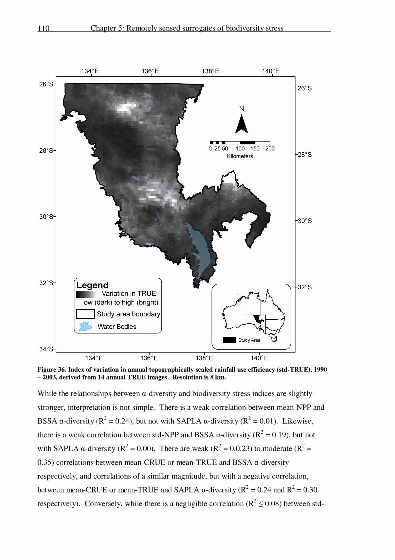
Chapter 5: Remotely sensed surrogates of biodiversity stress
110
Figure 36. Index of variation in annual topographically scaled rainfall use efficiency (std-TRUE), 1990
– 2003, derived from 14 annual TRUE images. Resolution is 8 km.
While the relationships between α-diversity and biodiversity stress indices are slightly
stronger, interpretation is not simple. There is a weak correlation between mean-NPP and
BSSA α-diversity (R2 = 0.24), but not with SAPLA α-diversity (R
2 = 0.01). Likewise,
there is a weak correlation between std-NPP and BSSA α-diversity (R2 = 0.19), but not
with SAPLA α-diversity (R2 = 0.00). There are weak (R
2 = 0.0.23) to moderate (R
2 =
0.35) correlations between mean-CRUE or mean-TRUE and BSSA α-diversity
respectively, and correlations of a similar magnitude, but with a negative correlation,
between mean-CRUE or mean-TRUE and SAPLA α-diversity (R2 = 0.24 and R
2 = 0.30
respectively). Conversely, while there is a negligible correlation (R2 ≤ 0.08) between std-
Chapter 5: Remotely sensed surrogates of biodiversity stress
111
CRUE or std-TRUE and BSSA α-diversity, there is a moderate correlation with a negative
correlation between std-CRUE or std-TRUE and SAPLA α-diversity (R2 = -0.33 and R
2 = -
0.40 respectively).
In most cases the index of topographically scaled rainfall use efficiency correlated more
strongly with α-diversity than the index of climatically distributed rainfall use efficiency.
5.4 Discussion
We proposed two surrogates of biodiversity stress based on the causes of and pressures on
biodiversity and validated these using an index of perennial vegetation species diversity.
Surrogate 1 was based on the hypothesis that the difference between net primary
production (NPP) and expected primary productivity (EPP) was an index of biodiversity
stress. Surrogate 2 was based on the hypothesis that overgrazing decreases average NPP
and rainfall use efficiency (RUE), and increases variation in NPP and RUE. Our validation
is based on an index of α-, β- or γ-diversity and review of the literature which suggested
that α- and γ-diversity decrease with increasing severity of grazing induced degradation.
Evaluation of the performance of Surrogate 1 is simple: our analysis found no relationship
between Surrogate 1 and woody perennial vegetation α-, β- or γ-diversity extracted from
either of the conventional vegetation surveys. Evaluation of Surrogate 2 is more difficult:
We found no consistent relationship between any form of species-diversity derived from
either conventional vegetation survey and any of the potential image indices of biodiversity
pressure. Some of our results supported the hypothesis that overgrazing decreases average
NPP and RUE: BSSA α-diversity decreased with decreasing average NPP, CRUE and
TRUE. However, some of our other results contradicted this hypothesis: SAPLA α-
diversity declined with increasing average CRUE and TRUE. Likewise, the hypothesis
that overgrazing increases variation in NPP and RUE is supported by some of our results
and contradicted by others: SAPLA α-diversity decreased with increasing temporal
variation in CRUE and TRUE, as expected; while contrary to expectations BSSA α-, β-
and γ-diversity all increased with increasing temporal variation in NPP. Finally, none of
our results supported the most important part of our hypothesis; that the proposed indices
of biodiversity pressure would co-vary with woody perennial γ-diversity.
Chapter 5: Remotely sensed surrogates of biodiversity stress
112
The lack of detected relationship between Surrogate 1 and vegetation species diversity may
be due to either of, or a combination of two factors; data limitations obfuscating the
relationship, or an un-accounted for source of variation preventing the water-energy
hypothesis from being the primary determinant of diversity in the study area. Likewise,
the complex relationship of Surrogate 2 to vegetation species diversity may be due to one
of two factors; the same data limitations suffered by Surrogate 1, or the difference in site
placement of the two vegetation surveys from which the species diversity index was
extracted. We will deal with the factors unique to Surrogates 1 and 2 first, and then
discuss the common data limitations.
Considering Surrogate 1 first; if another factor is similarly or more limiting to primary
production than the balance between water and energy availability, then we would expect
the relationship between Surrogate 1 and vegetation species diversity to be weak or non-
existent. We suggest that the variation in soils in the study area is such a factor.
The extreme age of soils and the internal drainage of the study area combine to provide
serious impediments to plant growth. The combination of these two factors means that
soils in the upper parts of catchments are heavily leached and contain only very small
amounts of soluble salts, while the lower parts of catchments are heavily salinised to the
point of forming salt-encrusted pans (Hubble et al. 1983). In addition to these general
problems, the specific soils covering the study area present their own unique obstacles to
plant growth: the deep sands suffer gross deficiencies of both major and minor elements;
the calcareous soils are strongly alkaline, with typical pH > 9 and sometimes suffering
zinc, iron or copper deficiencies; and most of the texture-contrast soils are low in
phosphorus and many are both saline and sodic (Northcote and Skene 1972; Hubble et al.
1983). Hence, the soils of the study area present many challenges to plant growth.
However, the study area is relatively vegetated, considering its aridity, and each soil type is
characterised by a specialised vegetation community adapted to dealing with the specific
challenges presented by that soil (Specht and Specht 1999).
Secondly, the complex relationship of Surrogate 2 to vegetation species diversity may
result from the differences in survey design, and hence site placement. To clarify the
following discussion we will briefly reiterate the differences in the two vegetation survey
Chapter 5: Remotely sensed surrogates of biodiversity stress
113
methodologies. Firstly, the surveys differ in intent and hence site placement: the BSSA is
an inventory survey, and where possible sites are placed in locations remote from water, to
avoid regions more heavily grazed by domestic stock; the SAPLA is a pastoral range
condition monitoring survey, all sites are placed within the piosphere to measure the
magnitude of grazing pressure. Secondly, surveyor expertise differs: the BSSA employs
botanical experts, while the SAPLA employs range monitoring professionals with some
botanical training.
All SAPLA sites are within the piosphere, and therefore grazed to some extent. Thus, the
intermediate disturbance hypothesis (Connell 1978; Menge and Sutherland 1987) may
explain the relationship between SAPLA α-diversity and average rainfall use efficiency.
Under this hypothesis, moderate degradation would reduce average rainfall use efficiency
and increase α-diversity, as compared to low degradation. Additionally, according to our
hypothesis, moderate degradation would increase variation in rainfall use efficiency and
decrease α-diversity, as compared to low degradation.
Alternatively, the BSSA is an inventory survey; sites are placed with the intent of
recording as many present species as possible. Hence, sites are generally placed in areas of
good condition remote from stock watering points. However, some sites must necessarily
be placed close to water, when the landscape type is by its very nature associated with
close proximity to water, or when the only accessible examples of a landscape type are
close to water. Thus we expect that BSSA sites might cover a wider range of grazing
conditions than SAPLA sites, from no grazing to heavily grazed. If this is the case, and we
do not invoke the intermediate disturbance hypothesis, then our original arguments would
explain the relationship between BSSA α-diversity, average net primary production and
average rainfall use efficiency.
However, we find these explanations unsatisfying. We can find no difference in vegetation
survey methodologies which would allow the invocation of the intermediate disturbance
hypothesis for one survey and not the other. Neither can we find an adequate explanation
for the increase in variation in net primary production with increasing BSSA α-, β- and γ-
diversity, which is contrary to our predictions. Ultimately all of the Surrogate 2
Chapter 5: Remotely sensed surrogates of biodiversity stress
114
correlations are weak, and the differential response of the BSSA and SAPLA α-diversity
casts doubt on the significance of any of our relationships.
We feel that the confusing and weak relationships derived in the validation of Surrogates 1
and 2 are the result of two factors. The first and more serious is the interpolation of the
rainfall and evapotranspiration surfaces used in the analyses. The second is that the
NOAA NDVI data, from which net primary production is calculated, is of a relatively
coarse spatial resolution in relation to the scale of variation in species diversity and grazing
management.
The rainfall surface is, as previously mentioned, interpolated from a minimum of 30
climate stations, only 22 of which are located inside the study area. Thus, the rainfall, and
hence evapotranspiration, at any given point is interpolated from data collected at stations
ranging from a few kilometres to several hundred kilometres away. As a result of this
interpolation from an originally low data density, the rainfall surfaces do not truly
represent any of the localised variation in rainfall. The study area does not experience
reliable seasonal rainfall, and localised thunderstorm activity can provide a significant
boost to annual rainfall in a small area. Likewise, orographic precipitation and rain-
shadowing are not represented in the interpolated rainfall, and could both influence rainfall
in the study area. Additionally, interpolation of rainfall from few climate stations will
mean that a localised extreme weather event over one of the climate stations can
significantly affect a large area of the rainfall surface. We believe such a localised event
caused a large circular area of extremely low rainfall, centred at 138.5° E, 29° S, in two
years rainfall surfaces. Such a severe absence of rainfall should have caused a visible
reduction of net primary production over a similar area, however none was visible. Thus,
while the SILO rainfall and evapotranspiration data (Jeffrey et al. 2001) is the best
available for the study area, it does not accurately reflect rainfall throughout our study area.
The NOAA NDVI data are likewise the best existing data of its type for the study area and
period. However, the smallest element of the NOAA NDVI data, the pixel, is 8 x 8 km (64
km2). This contrasts strongly with the scale of our species diversity measurements: BSSA
sites are 100 x 100 m (0.01 km2); SAPLA sites range from 100 to 200 m radius (0.03 –
0.13 km2). Thus the vegetation survey sites cover a very small proportion of a single
Chapter 5: Remotely sensed surrogates of biodiversity stress
115
NDVI pixel, and therefore the condition of either BSSA or SAPLA sites may not be
representative of the majority of the pixel area.
The NDVI pixel area is a good match to the area typically utilised by cattle, but not to the
area utilised by sheep. Cattle grazing is predominant in the north of the study area, and
cattle are expected to move as little as 4 km from water when forage is plentiful, and as
much as 20 km from water when forage is very scarce or in winter (Hodder and Low 1978;
Low et al. 1978). Given that the study area is amongst the most arid of Australia’s
rangelands, we therefore expect that forage will rarely be plentiful and that cattle will
usually utilise an area as large, or larger than, one NDVI pixel around a watering point.
Sheep, the grazing of which predominates in the south of the study area, utilise a smaller
portion of the landscape. In hot, dry conditions, and especially in chenopod shrublands
sheep must remain close to water, and forage range is reduced to 3 km (Lange 1969; Lynch
1974; Squires 1976; Squires 1978; Wilson and Graetz 1980). However, in cooler or wetter
weather sheep may graze further from watering points (Osborn et al. 1932; Wilson 1978).
We expect that the majority of grazing induced degradation will occur in hotter, dryer parts
of the year when the sheep grazing is focused in a smaller area. Therefore, the area
degraded by sheep grazing will be less than half of the area of one NDVI pixel, while the
rest of the pixel may cover non-grazed landscape. We would expect this mixture of grazed
and non-grazed landscape to reduce the impact of grazing induced degradation on NDVI in
the southern portion of the study area dominated by sheep grazing.
5.4.1 Summary
To summarise, we proposed two surrogates of biodiversity stress: Surrogate 1, based on
the well supported Productivity Theory (O'Brien 1993; Whittaker et al. 2003; Cardinale et
al. 2006) and the difference between indices of net and expected primary production; and
Surrogate 2, based on average and variation in net primary production and rainfall use
efficiency. We validated Surrogates 1 and 2 against an index of woody perennial
vegetation α-, β- and γ-diversity, assuming that prolonged biodiversity stress would cause
low vegetation species diversity.
We have thoroughly tested Surrogates 1 and 2 in the South Australian rangelands with the
best available remotely sensed data and climate data for the study area and period. Our
Chapter 5: Remotely sensed surrogates of biodiversity stress
116
analysis did not reveal a convincing link between either Surrogate 1 or 2 and vegetation
species diversity. However, we feel that the analysis was hampered to a large degree by
the rainfall data, which is interpolated from climate stations up to several hundred
kilometres away. Additionally, the relatively coarse scale of the NOAA NDVI data, and
the fine scale over which sheep graze may have hampered detection of the impact of sheep
grazing. Finally, analysis by IBRA sub-regions accounted for some, but not all, of the
influence of soil type on vegetation community. Differing amounts of soil variation in
IBRA sub-regions may have confounded evaluation of Surrogate 1 by providing a source
of variation in species diversity as or greater than that caused by primary productivity.
It is difficult to draw any conclusions regarding rainfall use efficiency, due to the
limitations of the rainfall data. However, the NOAA NDVI data does not impose similar
limitations in drawing conclusions about net primary productivity. The area utilised
around water points by cattle grazing is a good match with the scale of the NDVI imagery,
and sheep grazing is affects a smaller but still substantial portion of an NDVI pixel.
Therefore, it is interesting that we did not find the expected link between grazing induced
degradation, decreased average net primary production and increased temporal variation in
net primary production. It appears that this link, found elsewhere in Australia and other
parts of the world, is substantially weaker or does not exist in the study area.
This analysis has highlighted the lack of high resolution climate data in the Australian
rangelands. This gross deficiency must be addressed before many forms of environmental
modelling can assist in range management at any but the broadest of scales; including
understanding and mitigating the effects of climate change. We recommend that the
resolution of climate data in the rangelands should be improved, to better reflect meso-
scale variation.
5.5 References
Andres, L., W. A. Salas and D. Skole (1994) Fourier analysis of multi-temporal AVHRR data applied to a land cover classification. International Journal of Remote Sensing 15(5): 1115 - 1121. Asrar, G., E. Kanemasu, R. Jackson and P. Printer (1985) Estimation of total above-ground phytomass production using remotely sensed data. Remote Sensing of Environment 17: 211-220. Badgley, C. and D. L. Fox (2000) Ecological biogeography of North America mammals: species density and ecological structure in relation to environmental gradients. Journal of Biogeography 27: 1437-1467.
Chapter 5: Remotely sensed surrogates of biodiversity stress
117
Box, E., B. Holben and V. Kalb (1989) Accuracy of the AVHRR Vegetation Index as a predictor of biomass, primary productivity and net CO2 flux. Vegetatio 80: 71-89.
Cardinale, B. J., D. S. Srivastava, J. E. Duffy, J. P. Wright, A. L. Downing, M. Sankaran and C. Jouseau (2006) Effects of biodiverstiy on the functioning of trophic groups and ecosystems. Nature 443: 989-992. Clarke, K. D., M. M. Lewis and B. Ostendorf (submitted) Additive partitioning of rarefaction curves: removing the influence of sampling on species-diversity in vegetation surveys. Ecological Indicators?(?): ? Connell, J. H. (1978) Diversity in tropical rain forests and coral reefs. Science 199(4335): 1302-1310.
Costanza, R., R. d'Arge, R. de Groot, S. Farber, M. Grasso, B. Hannon, K. Limburg, S. Naeem, R. O'Neill, J. Paruelo, R. Raskin, P. C. Sutton and M. van den Belt (1997) The value of the world's ecosystem services and natural capital. Nature 387: 253-260. Currie, D. J. (1991) Energy and large-scale patterns of animal-species and plant-species richness. American Naturalist 137(1): 27-49. Currie, D. J. and V. Paquin (1987) Large-scale biogeographical patterns of species richness of trees. Nature 329: 326-331.
Gallant, J. C. and T. I. Dowling (2003) A multiresolution index of valley bottom flatness for mapping depositional areas. Water Resources Research 39(12). Hawkins, B. A. and E. E. Porter (2003) Does herbivore diversity depend on plant diversity? The case of California butterflies. American Naturalist 161(1): 40-49. Hawkins, B. A. and E. E. Porter (2003) Water-energy balance and the geographic pattern of species richness of western
Palearctic butterflies. Ecological Entomology 28: 678-686. Hawkins, B. A., E. E. Porter and J. A. F. Diniz-Filho (2003) Productivity and history as predictors of the latitudinal diversity gradient of terrestrial birds. Ecology 84(6): 1608-1623. Hobbins, M. T., J. A. Ramirez, T. C. Brown and L. H. J. M. Claessens (2001) The complementary relationship in estimation of regional evapotranspiration: The Complementary Relationship Areal Evapotranspiration and Advection-Aridity models. Water Resources Research 37(5): 1367-1387.
Hodder, R. M. and W. A. Low (1978) Grazing distribution of free-ranging cattle at three sites in the Alice Springs district, central Australia. The Australian Rangeland Journal 1: 95-105. Holben, B. N. (1986) Characteristics of maximum-value composite images from temporal AVHRR data. International Journal of Remote Sensing 7(11): 1417-1434. Holm, A. M., I. W. Watson, W. A. Loneragan and M. A. Adams (2003) Loss of patch-scale heterogeneity on primary
productivity and rainfall-use efficiency in Western Australia. Basic and Applied Ecology 4: 569-578. Hubble, G. D., R. F. Isbell and K. H. Northcote (1983) Features of Australian soils. Soils: an Australian viewpoint, CSIRO: Melbourne / Academic Press: London. Huete, A. R. and R. Jackson (1987) Suitability of spectral indices for evaluating vegetation characteristics on arid rangelands. Remote Sensing of Environment 23: 213-232.
Jeffrey, S. J., J. O. Carter, K. M. Moodie and A. R. Beswick (2001) Using spatial interpolation to construct a comprehensive archive of Australian climate data. Environmental Modelling and Software 16(4): 309-330. Lambin, E. F. and A. H. Strahler (1994) Change-vector analysis in multitemporal space: a tool to detect and categorize land-cover change processes using high temporal-resolution satellite data. Remote Sensing of Environment 48(2): 231-244. Lange, R. T. (1969) The piosphere: sheep track and dung patterns. Journal of Range Management 22: 396-400.
Low, W. A., R. M. Hodder and D. E. Abel (1978) Watering behaviour of British breed cattle in central Australia. Studies of the Australian Arid Zone III. Water in rangelands. K. M. W. Howes. Perth, Australia, CSIRO.

Chapter 5: Remotely sensed surrogates of biodiversity stress
118
Lynch, J. J. (1974) Merino sheep: some factors affecting their distribution in very large paddocks. The behaviour of Ungulates and its relation to management. V. Geist and F. Walther. Morges, Switzerland, International union for the conservation of nature new series.
Menge, B. A. and J. P. Sutherland (1987) Community Regulation: Variation in Disturbance, Competition, and Predation in Relation to Environmental Stress and Recruitment doi:10.1086/284741. The American Naturalist 130(5): 730. Morton, F. I. (1983) Operational estimates of areal evapotranspiration and their significance to the science and practice of hydrology. Journal of Hydrology 66: 1-76.
Northcote, K. H. and J. K. M. Skene (1972) Australian soils with saline and sodic properties. CSIRO Soil Publications. O'Brien, E. (2006) Biological relativity to water-energy dynamics. Journal of Biogeography 33: 1868-1888. O'Brien, E. M. (1993) Climatic gradients in woody plant species richness: towards an explanation based on an analysis of Southern Africa's woody flora. Journal of Biogeography 20: 181-198. O'Brien, E. M. (1998) Water-energy dynamics, climate, and prediction of woody plants species richness: an interim general model. Journal of Biogeography 25: 379-398.
Osborn, T. G., J. G. Wood and T. B. Paltridge (1932) On the growth and reaction to grazing of the perennial saltbush Atriplex vesicarium: an ecological study of the biotic factor. Proceedings of the Linnean Society of New South Wales 57: 377-402. Rasmussen, M. S. (1998) Developing simple, operational, consistent NDVI-vegetation models by applying environmental and climatic information: Part I. Assessment of net primary production. International Journal of Remote Sensing 19(1): 97-117.
Reed, B. C., T. R. Loveland and L. L. Tieszen (1996) An approach for using AVHRR data to monitor U.S. Great Plains grasslands. Geocarto International 11(3): 13-22. Ricotta, C., G. Avena and A. De Palma (1999) Mapping and monitoring net primary productivity with AVHRR NDVI time-series: statistical equivalence of cumulative vegetation indices. Isprs Journal of Photogrammetry and Remote Sensing 54(5-6): 325-331.
Sarkar, S. (2002) Defining "Biodiversity"; Assessing Biodiversity. The Monist 85(1): 131-155. Smyth, A. K., V. H. Chewings, G. N. Bastin, S. Ferrier, G. Manion and B. Clifford (2004) Integrating historical datasets to prioritise areas for biodiversity monitoring? Australian Rangelands Society 13th Biennial Conference: "Living in the outback", Alice Springs, Northern Territory. Specht, R. L. and A. Specht (1999) Australian plant communities: dynamics of structure, growth and biodiversity, Kyodo, Singapore.
Squires, V. R. (1976) Walking, watering and grazing behaviours of Merino Sheep on two semi-arid rangelands in south-west New South Wales. The Australian Rangeland Journal 1: 13-23. Squires, V. R. (1978) Distance trailed to water and livestock response. Proceedings of the First International Rangelands Congress, Denver, USA, Society for Range Management. Tucker, C., B. Holben, J. Elgin and J. McMurtrey (1981) Remote Sensing of Total Dry-Matter Accumulation in Winter
Wheat. Remote Sensing of Environment 11: 171-189. Tucker, C. and P. J. Sellers (1986) Satellite remote sensing of primary production. Int. J. Remote Sensing 7(11): 1395-1416. Whittaker, R. J., K. J. Willis and R. Field (2003) Climatic-energetic explanations of diversity: a macroscopic perspective. Macroecology: concepts and consequences. T. M. Blackburn and K. J. Gaston. Oxford, Blackwell Science: 107-129. Wilson, A. D. (1978) Water requirements of sheep. Studies of the Australian Arid Zone: Water in Rangelands. K. M. W.
Howes. Perth, Australia, CSIRO. 3: 178-189.

Chapter 5: Remotely sensed surrogates of biodiversity stress
119
Wilson, A. D. and R. D. Graetz (1980) Cattle and sheep production on Atriplex vesicaria (saltbush) community. Australian Journal of Agricultural Research 31: 369-378.
Chapter 6: Discussion and conclusions
120
Chapter 6: Discussion and conclusions
6.1 Introduction
The overarching goal of this thesis was to contribute to the development of better tools for
the monitoring of biodiversity in the Australian rangelands. Specifically, this work aimed
to extract indices capable of measuring and/or monitoring biodiversity from vegetation
quadrat survey data and remotely sensed data over the Australian rangelands.
This thesis has contributed significantly to this goal by providing new tools for biodiversity
measurement, including a method for extracting α-, β- and γ-diversity from vegetation
quadrat survey data and removing the influence of sampling effort, and two remote sensing
based indices of pressure on biodiversity. Additionally, this work has contributed to the
research goal by raising awareness of the limitations of vegetation quadrat surveys and
hence accelerating the development of more robust and meaningful analyses of vegetation,
and by identifying limitations in climate monitoring data, which if addressed may allow for
better modelling of biodiversity in the arid rangelands.
Our analysis of false-negative errors in conventional vegetation survey data provided an
important cautionary lesson on the limitations of such data in the study area (Chapter 3).
Significant rates of false-negative errors remained, even after limiting analysis to the most
persistent, most detectable species. Therefore, any biodiversity metric derived from such
survey data collected in the study area must account for the expected false-negative errors
or be seriously flawed.
In Chapter 4, a regional index of vegetation α-, β- and γ-species diversity was derived from
extensive vegetation quadrat survey data, as a surrogate for biodiversity. This index
accounted for regional differences in sampling effort, and the γ-diversity index is
theoretically insensitive to false-negative errors.
Finally, two spatially distributed surrogates of biodiversity stress, based on the causes of
and pressures on biodiversity, were derived from the best available remotely sensed and
climate data (Chapter 5). These surrogates were thoroughly tested against the index of α-,
β- and γ-diversity, and no convincing link was found between either surrogate and
Chapter 6: Discussion and conclusions
121
vegetation species diversity. However, this analysis was probably limited by the available
climate data.
Thus, this thesis has addressed the original goal identified in Chapter 1. The specific
contributions to knowledge made by each of the research chapters is discussed in Section
2; the broader implications of the research findings, and the factors which limit the extent
to which the findings may be generalised are discussed in Section 3.
6.2 Summary of specific contributions to knowledge
6.2.1 False-negative errors in a survey of vegetation species
The Biological Survey of South Australia (BSSA) was identified as the best available
biodiversity survey in the study region. This prompted an evaluation of the BSSA data to
determine their quality and potential to supply a ground based biodiversity indicator for
comparison with remotely sensed surrogates of biodiversity. This lead to the analysis in
Chapter 3, the major aim of which was to conservatively estimate false-negative error rates
of the perennial vegetation species data collected by the BSSA. It was hoped that
quantification of false-negative error rates would facilitate the development of corrective
measures, and therefore the derivation of more meaningful information from the BSSA
data.
The analysis was performed on data collected from four BSSA sites visited twice yearly
for eight years. Even after limiting the study to the most easily-detected perennial
vegetation species, and controlling for observer skill, we revealed frequent false-negative
errors by all surveyors, at all sites, for all species examined. Thus, we demonstrated in the
study area that even highly detectable vegetation species often have detection probabilities
significantly less than one.
In addition to the BSSA, there are other broad scale vegetation surveys in the region, such
as the South Australian Pastoral Lease Assessment (SAPLA), that generate vegetation data
which may be used for similar purposes, and which may also suffer from false-negative
errors. An evaluation of the differences between the BSSA and the SAPLA led us to
expect higher rates of false-negative errors in the SAPLA.

Chapter 6: Discussion and conclusions
122
The problem of false negative errors in vegetation surveys has not featured prominently in
the literature, unlike false negative errors in fauna surveys, which has received significant
attention (see MacKenzie et al. 2002; Tyre et al. 2003; Gu and Swihart 2004; MacKenzie
2005; MacKenzie 2005). It appears that vegetation species are assumed to be highly or
perfectly detected by conventional vegetation surveys. We have demonstrated that this
assumption is not necessarily warranted, and would recommend that vegetation surveys
adopt measures to gauge the detectability of species, and to correct for false-negative
errors, as is already done in some fauna surveys.
Finally, for more mundane reasons we would also caution against the use of raw vegetation
quadrat survey data to assess regional variation in biodiversity. The data collected by these
surveys may not be representative without additional analysis, due to the small size of the
quadrats in relation to the extensive scale of landscapes. Additionally, differences in
sampling effort may confound regional measures which fail to account for the influences
of sampling effort.
6.2.2 Additive partitioning of rarefaction curves species diversity surrogate
The aim of Chapter 4 was to develop a biodiversity metric free from the influence of
sampling effort. The γ-diversity of woody-perennial vegetation was identified as an
estimator-surrogate for biodiversity, and we hypothesised that rarefaction to a common
sampling effort and extraction of α-, β- and γ-diversity through additive partitioning of
species diversity would remove the influence of sampling effort.
The analysis demonstrated that rarefaction to a common sampling effort did not completely
remove the influence of sampling effort. However, the influence of sampling effort on γ-
diversity was predictable, and therefore it was possible to correct for the influence.
Additionally, this index of woody perennial vegetation γ-diversity theoretically minimises
the influence of false negative errors, especially for well-sampled regions.
While the index developed in Chapter 4 is specific to the study area, the method for
creating the index is not. This method is transferable and can conceivably be employed to
extract a sampling effort corrected measure of γ-diversity from any vegetation data
obtained from site-based surveys following prescribed methodologies.
Chapter 6: Discussion and conclusions
123
Furthermore, our work answers the call by Fleishman et al. (2006) to standardize measures
of species richness for differences in survey effort. However we have demonstrated a
significant point not previously reported in the literature, that rarefaction alone does not
adequately control for the influence of sampling effort. If this relationship exists in other
areas, then interpolation or extrapolation of rarefaction relationships, a common use of
rarefaction, will produce erroneous results.
However, this woody perennial vegetation γ-diversity does not address the need for a
spatially extensive, fine scale measure of biodiversity at the scale of the Australian
rangelands. The aggregation of point data to large regions, a necessary part of this index,
produces spatially coarse results.
6.2.3 Remotely sensed biodiversity stress surrogates
The major aim of Chapter 5 was to develop an index of pressure on biodiversity capable of
covering the extensive Australian rangelands at a fine scale. We developed two indices of
biodiversity stress based on the causes of and pressures on biodiversity, and produced from
the best available remotely sensed and climatic data. Surrogate 1 was based on the
supported Productivity Theory (O'Brien 1993; Whittaker et al. 2003; Cardinale et al. 2006)
and the difference between indices of net and expected primary production; and Surrogate
2, based on average and variation in net primary production and rainfall use efficiency.
We validated Surrogates 1 and 2 against the index of woody perennial vegetation α-, β-
and γ-diversity developed in Chapter 4. The rationale of the validation was based on the
literature which suggests that that α- and γ-diversity decrease with increasing severity of
grazing induced degradation, the most prevalent source of biodiversity stress in the study
area.
Surrogates 1 and 2 were thoroughly tested with the best available remotely sensed and
climate data for the study area and period. There was no relationship between the first
surrogate and woody perennial α-, β- or γ-diversity extracted from either the BSSA or the
SAPLA data. The relationship of the second surrogate to the validation data was more
complex. While some of the results supported the hypothesis that overgrazing decreases α-
diversity and average NPP and RUE, other results did not. Importantly, none of our results
supported the most important part of our hypothesis; that the proposed indices of
Chapter 6: Discussion and conclusions
124
biodiversity pressure would co-vary with woody perennial γ-diversity. Thus, the analysis
did not reveal a convincing link between either Surrogate 1 or 2 and vegetation species
diversity. However, the analysis was hampered to a large degree by the rainfall data,
which is interpolated from climate stations up to several hundred kilometres away.
Additionally, while soil heterogeneity probably influences vegetation γ-diversity in the
study area (Chapter 2, Section 2.1.4), we were not able to account for this effect. While
the extent of the study area and the coarse scale of available soil maps precluded
meaningful analysis, stratification of analysis by IBRA sub-region has accounted for the
influence of soil heterogeneity on vegetation diversity as best as possible.
While the rainfall data limited the conclusions which could be drawn from these analyses,
the satellite data was of sufficient quality to allow a robust examination of net primary
production. Therefore, it is interesting that the analysis found no link between grazing
induced degradation (measured by reduced α- or γ-diversity), decreased average net
primary production and increased temporal variation in net primary production, contrary to
expectations from the literature (see Le Houerou 1984; Snyman and Fouché 1993; Snyman
1997; Snyman 1998; Holm et al. 2002; Holm et al. 2003).
It is important to note that this climate data has been identified as a limiting factor by other
research into biodiversity surrogates in the study area. Smyth et al. (2007) attributed the
inability of their study to detect the expected relationship between vegetation species
diversity (as a surrogate for biodiversity) and any of several potential biodiversity
surrogates to the low resolution of the climate information in the study area.
6.3 Limitations to generalisation
While the work presented in this thesis made some important contributions to knowledge,
the extent to which the conclusions of this work can be generalised are limited in scope.
This section covers the specific limitations to generalisation of each of the research
chapters.
Chapter 6: Discussion and conclusions
125
6.3.1 False-negative errors in a survey of vegetation species
While the analysis of false-negative errors presented in Chapter 3 was performed on data
collected by a specific vegetation quadrat survey, the Biological Survey of South Australia
(BSSA), the methods used by this survey are typical of vegetation quadrat surveys.
Therefore, the results of this analysis should be considered quite general: any vegetation
survey may contain significant false-negative errors.
By critically evaluating the differences between the BSSA and another vegetation survey
in the study area, the South Australian Pastoral Lease Assessment (SAPLA), it was
possible to estimate the relative level of false-negative errors in the SAPLA. All
differences between the BSSA and SAPLA lead to an expectation of higher rates of false-
negative errors in the SAPLA.
Similar comparisons of the methodology of BSSA and other vegetation surveys of interest
may help gauge the probable magnitude of false-negative errors in these other surveys.
However, such comparisons should only be used as a guide, and should not replace a
proper analysis of false-negative error rates.
6.3.2 Diversity indices
The diversity indices derived in Chapter 4 are specific to the study area, the taxa studied,
and the vegetation survey method, and should not be applied outside of these bounds.
However, the methods used to derive the diversity indices are wholly transferable, and
provides a theoretically sound framework for deriving an indicator of α-, β- and γ-diversity
which is comparable between regions of different sampling effort. This index can
conceivably be generated from any vegetation quadrat survey data obtained within a
prescribed methodology.
Through the use of additive partitioning, α-, β- and γ-diversity are expressed in the same
units of species richness, and are therefore directly comparable. While the indices do not
directly model and account for false-negative errors in the vegetation survey data, the
methods used theoretically reduce these errors to varying degrees depending on the type of
diversity. The γ-diversity index is theoretically insensitive to false-negative errors, and
becomes even less sensitive at higher sampling efforts: a species must be recorded at only
Chapter 6: Discussion and conclusions
126
one site in a region to contribute to γ-diversity. The index of α-diversity is theoretically
vulnerable to the effect of false-negative errors. Although steps have been taken to
minimise the number of false-negative errors contained in the vegetation survey data by
limiting it to persistent perennial species, the analysis in Chapter 3 demonstrated that the
data were still likely to contain significant rates of false-negative errors. Finally, β-
diversity is generated from α-, and γ-diversity, through additive partitioning. Therefore,
the sensitivity of β-diversity to false-negative errors will be an average of the sensitivity of
α-, and γ-diversity: β-diversity is less sensitive than α-, and more sensitive than γ-diversity.
As with γ-diversity, β-diversity will become less sensitive to false-negative errors at higher
sampling efforts.
While the diversity indices derived in Chapter 4 are in the strictest sense specific to the
taxon studied, this ignores the issue of surrogacy. This thesis has made the argument that
one taxon may act as a surrogate for one or several other taxa (see Chaper 1, section 1
Motivation for the research; Chapter 3, section 1 Introduction; Chapter 4, section 1
Introduction), and the literature supports the use of the use of cross-taxon biodiversity
surrogates (Rodrigues and Brooks 2007). In this sense, the diversity indices are not
specific to the taxa studied, but may be considered indicative of overall taxon diversity.
6.3.3 Remotely sensed surrogates of biodiversity stress
The two surrogates derived in Chapter 5 are theoretically sound measures of grazing
pressure on biodiversity, and are calculated from reliable, calibrated data. Therefore, it
would be reasonable to compare surrogate values derived in the study area to values
derived elsewhere with the same surrogate, from similar quality data; at the same scale;
and if grazing pressure is a major source of biodiversity pressure. However, the limitations
of the climate data used in the generation of the surrogates should be considered before
such comparisons are made: the climate data are interpolated from climate stations up to
several hundred kilometres away.
Chapter 6: Discussion and conclusions
127
6.4 Broader implications
6.4.1 False-negative errors in a survey of vegetation species
The analysis presented in Chapter 3 has implications for vegetation surveying in general.
The results suggest that a single site-survey may miss some of the most detectable
vegetation species, and will probably miss an even greater proportion of the less detectable
vegetation species. This finding has serious ramifications for the interpretation of
vegetation survey data as well as those managing the surveys.
The data collected by quadrat vegetation surveys are often analysed on the assumption that
they are presence-absence data (e.g. Brandle 1998; Robinson and Armstrong 1999;
Brandle 2001; Smyth et al. 2007). However the work presented herein suggests that this
assumption should be checked: these data may only be reasonably considered presence-
only data. The use of an inappropriate analysis, the assumptions of which are not met, will
produce erroneous results. Hence, this finding will guide the use of more appropriate
analyses of vegetation survey data in the future, and a concurrent increase in the quality of
knowledge extracted from vegetation surveys.
For managers of vegetation surveys the ramifications are methodological, as many
vegetation surveys aim to collect presence-absence data. The high frequency of false-
negative errors revealed by Chapter 3 demonstrates that data collected by the vegetation
survey examined, and by extension the data collected by similar vegetation surveys, may
only reasonably be considered presence-only data. If it is essential that the data collected
by a survey can be considered presence-absence data, then simple alterations to that
surveys methodology should allow for the measurement and correction of false-negative
errors. In particular, we would recommend the same measures that are taken to counteract
false-negative errors in fauna surveying: multiple sampling occasions at each site within a
short time (MacKenzie et al. 2002; Gu and Swihart 2004), specifically three repeat visits
(Tyre et al. 2003).
6.4.2 Diversity indices
Rarefaction is commonly used to standardise sampling effort for comparison between
populations. The analysis in Chapter 4 revealed that, at least in the study area, rarefaction
Chapter 6: Discussion and conclusions
128
did not wholly remove the influence of sampling effort on γ-diversity. While determining
the cause of this relationship was beyond the scope of the work in Chapter 4, it was
hypothesised that the non-detection errors identified in Chapter 3 may be the source of the
relationship between rarefied γ-diversity and sampling effort. As a result of this work,
rarefaction should not be used to control for differences in sampling effort without
additional testing to determine whether there is any residual influence from sampling
effort.
6.4.3 Remotely sensed surrogates of biodiversity stress
While there was no convincing link between the surrogates of biodiversity stress derived in
Chapter 5 and woody perennial vegetation α-, β- or γ-diversity, the analysis was hampered
by the low resolution of the available climate data. The surrogates are theoretically sound,
and could be applied in any region in which the assumptions of their theoretical framework
holds: arid to semi-arid rangelands.
While these surrogates need to be evaluated with adequate climate data, they offer great
potential for biodiversity management in arid and semi-arid rangelands. The surrogates are
derived from low-cost, extensive data, and are relatively easily produced. An adequate,
extensive measure of biodiversity would provide important information, and assist in the
management of rangelands for biodiversity conservation.
6.5 Recommendations and future research
The following areas of necessary research were identified through the work presented in
this thesis.
• Assessment of the extent of false-negative errors in vegetation quadrat surveys is
necessary to identify which surveys are more or less likely to contain significant
false-negative errors, and therefore when to include false-negative error mitigation
in survey methodology design.
• To minimise the impact of false-negative errors on vegetation quadrat surveys,
error mitigation strategies need to be evaluated so that appropriate
recommendations can be made.
Chapter 6: Discussion and conclusions
129
• To allow the re-interpretation and valuation of past analyses, work should be
undertaken to quantify the impact on analyses of treating presence-only data as
presence-absence data.
• The extent to which rarefaction to a common sampling effort still suffers residual
influence from sampling effort needs to be evaluated in different taxa and in data
collected by different survey methodologies.
• The source of the residual influence of sampling effort after rarefaction to a
common sampling effort should be identified.
• To evaluate the extent to which they may be generalised, the measures developed in
this thesis to extract sampling effort corrected measures of α-, β- and γ-diversity
should be employed in other regions.
• The generation of α-, β- and γ-diversity surfaces in sample rich regions through the
use of a moving window and custom additive-partitioning-rarefaction software
would produce more easily used, contiguous data, and should be investigated.
• The efficacy of the surrogates of biodiversity stress should be evaluated in regions
where adequate climate data are available.
• The resolution of climate data in general and specifically in the Australian
rangelands should be increased to facilitate better environmental modelling and
management.
• The development of other remotely sensed surrogates of biodiversity should be
investigated, to address the need for spatially comprehensive tools for monitoring
biodiversity across the globe.
• Examine the relationship between total net primary production (TNPP) and total
expected primary production (TEPP) with quantile regression to determine whether
there is a strong positive relationship between TEPP and the upper quantiles of
TNPP, and a weaker relationship at lower quantiles, as predicted by the hypothesis
on which Surrogate 1 was based.
Chapter 6: Discussion and conclusions
130
6.6 Conclusions
This thesis has contributed to the measurement and monitoring of biodiversity. The
identification of false-negative errors as a cause for concern will allow future analyses of
the vegetation survey data to adopt methods to counteract these errors, and hence extract
more robust information. The method for extracting sampling effort corrected indices of
α-, β- and γ-diversity allow for the examination and comparison of species diversity across
regions, regardless of differences in sampling effort. These indices are not limited to
rangelands, and can be extracted from any vegetation quadrat survey data obtained within a
prescribed methodology. Therefore, these tools contribute to global biodiversity
measurement and monitoring. Finally, the remotely sensed surrogates of biodiversity are
theoretically sound and applicable in any rangeland where over-grazing is a significant
source of degradation. However, because the evaluation of these surrogates in this thesis
was hampered by available data, further testing is necessary.
6.7 References
Brandle, R., Ed. (1998) A biological survey of the north west Flinders Ranges, South Australia, Dec-1997, Biological Survey and Research, Department for Environment, Heritage and Aboriginal Affairs, South Australia.
Brandle, R., Ed. (2001) A biological survey of the Flinders Ranges, South Austrlai 1997-1999, Biodiversity Survey and Monitoring, National Parks and Wildlife, South Australia, Department for Environment and Heritage. Cardinale, B. J., D. S. Srivastava, J. E. Duffy, J. P. Wright, A. L. Downing, M. Sankaran and C. Jouseau (2006) Effects of biodiverstiy on the functioning of trophic groups and ecosystems. Nature 443: 989-992. Fleishman, E., R. F. Noss and B. R. Noon (2006) Utility and limitations of species richness metrics for conservation
planning. Ecological Indicators 6(3): 543-553. Gu, W. and R. K. Swihart (2004) Absent or undetected? Effects of non-detection of species occurrence on wildlife-habitat models. Biological Conservation 116(2): 195-203. Holm, A. M., W. A. Loneragan and M. A. Adams (2002) Do variations on a model of landscape function assist in interpreting the growth response of vegetation to rainfall in arid environments? Journal of Arid Environments 50: 23-52.
Holm, A. M., I. W. Watson, W. A. Loneragan and M. A. Adams (2003) Loss of patch-scale heterogeneity on primary productivity and rainfall-use efficiency in Western Australia. Basic and Applied Ecology 4: 569-578. Le Houerou, H. N. (1984) Rain use efficiency: a unifying concept in arid-land ecology. Journal of Arid Environments 7: 213-247. MacKenzie, D. I. (2005) Improving inferences in popoulation studies of rare species that are detected imperfectly. Ecology 86(5): 1101-1113.
MacKenzie, D. I. (2005) What are the issues with presence-absence data for wildlife managers? Journal of Wildlife Management 69(3): 849-860. MacKenzie, D. I., J. D. Nichols, G. B. Lachman, S. Droege, J. A. Royle and C. A. Langtimm (2002) Estimating site occupancy rates when detection probabilities are less than one. Ecology 83(8): 2248-2255.
Chapter 6: Discussion and conclusions
131
O'Brien, E. M. (1993) Climatic gradients in woody plant species richness: towards an explanation based on an analysis of Southern Africa's woody flora. Journal of Biogeography 20: 181-198.
Robinson, A. C. and D. M. Armstrong, Eds. (1999) A biological survey of Kangaroo Island, South Austrlia, 1989 & 1990, Herritage and Biodiversity Section, Department for Environment, Heritage and Aboriginal Affairs, South Australia. Rodrigues, A. S. L. and T. M. Brooks (2007) Shortcuts for biodiversity conservation planning: the effectiveness of surrogates. Annual Review of Ecology, Evolution, and Systematics 38(1): 713-737. Smyth, A. K., R. Brandle, A. Brook, V. H. Chewings, M. Fleming and J. L. Read (2007) Methods for identifying,
selecting and interpreting indicators for assessing biodiversity condition in desert Australia, using the Stony Plains bioregion as a case study, Desert Knowledge Cooperative Research Centre. Snyman, H. A. (1997) The influence of range condition on the hydrological characteristics in semi-arid rangeland. The XVIII International Grassland Congress. Snyman, H. A. (1998) Dynamics and sustainable utilization of rangeland ecosystems in arid and semi-arid climates of southern Africa. Journal of Arid Environments 39(4): 645-666.
Snyman, H. A. and H. J. Fouché (1993) Estimating seasonal herbage production of a semi-arid grassland based on veld condition, rainfall, and evapotranspiration. African Journal of Range and Forage Science 10(1): 21-24. Tyre, A. J., B. Tenhumberg, S. A. Field, D. Niejalke, K. Parris and H. P. Possingham (2003) Improving precision and reducing bias in biological surveys: estimating false-negative error rates. Ecological Applications 13(6): 1790-1801. Whittaker, R. J., K. J. Willis and R. Field (2003) Climatic-energetic explanations of diversity: a macroscopic perspective. Macroecology: concepts and consequences. T. M. Blackburn and K. J. Gaston. Oxford, Blackwell Science: 107-129.
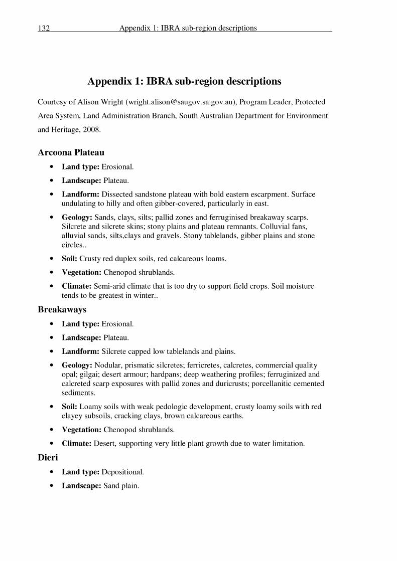
Appendix 1: IBRA sub-region descriptions
132
Appendix 1: IBRA sub-region descriptions
Courtesy of Alison Wright ([email protected]), Program Leader, Protected
Area System, Land Administration Branch, South Australian Department for Environment
and Heritage, 2008.
Arcoona Plateau
• Land type: Erosional.
• Landscape: Plateau.
• Landform: Dissected sandstone plateau with bold eastern escarpment. Surface
undulating to hilly and often gibber-covered, particularly in east.
• Geology: Sands, clays, silts; pallid zones and ferruginised breakaway scarps.
Silcrete and silcrete skins; stony plains and plateau remnants. Colluvial fans,
alluvial sands, silts,clays and gravels. Stony tablelands, gibber plains and stone
circles..
• Soil: Crusty red duplex soils, red calcareous loams.
• Vegetation: Chenopod shrublands.
• Climate: Semi-arid climate that is too dry to support field crops. Soil moisture
tends to be greatest in winter..
Breakaways
• Land type: Erosional.
• Landscape: Plateau.
• Landform: Silcrete capped low tablelands and plains.
• Geology: Nodular, prismatic silcretes; ferricretes, calcretes, commercial quality
opal; gilgai; desert armour; hardpans; deep weathering profiles; ferruginized and
calcreted scarp exposures with pallid zones and duricrusts; porcellanitic cemented
sediments.
• Soil: Loamy soils with weak pedologic development, crusty loamy soils with red
clayey subsoils, cracking clays, brown calcareous earths.
• Vegetation: Chenopod shrublands.
• Climate: Desert, supporting very little plant growth due to water limitation.
Dieri
• Land type: Depositional.
• Landscape: Sand plain.
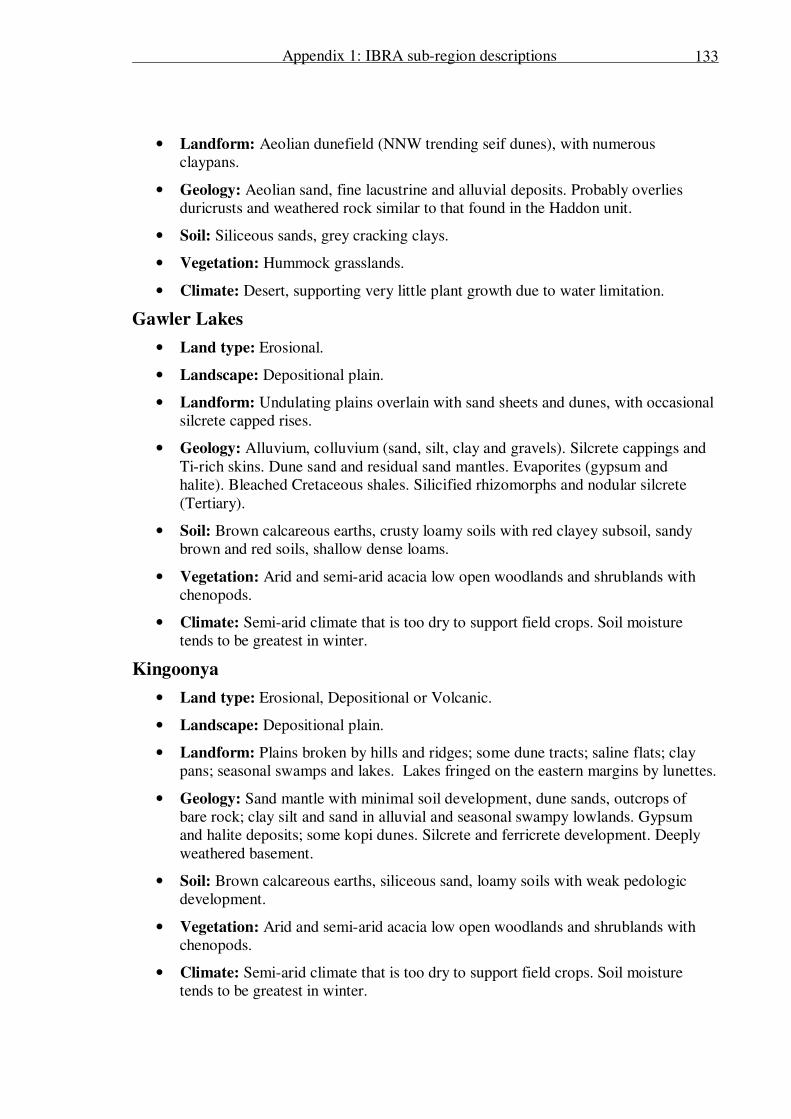
Appendix 1: IBRA sub-region descriptions
133
• Landform: Aeolian dunefield (NNW trending seif dunes), with numerous
claypans.
• Geology: Aeolian sand, fine lacustrine and alluvial deposits. Probably overlies
duricrusts and weathered rock similar to that found in the Haddon unit.
• Soil: Siliceous sands, grey cracking clays.
• Vegetation: Hummock grasslands.
• Climate: Desert, supporting very little plant growth due to water limitation.
Gawler Lakes
• Land type: Erosional.
• Landscape: Depositional plain.
• Landform: Undulating plains overlain with sand sheets and dunes, with occasional
silcrete capped rises.
• Geology: Alluvium, colluvium (sand, silt, clay and gravels). Silcrete cappings and
Ti-rich skins. Dune sand and residual sand mantles. Evaporites (gypsum and
halite). Bleached Cretaceous shales. Silicified rhizomorphs and nodular silcrete
(Tertiary).
• Soil: Brown calcareous earths, crusty loamy soils with red clayey subsoil, sandy
brown and red soils, shallow dense loams.
• Vegetation: Arid and semi-arid acacia low open woodlands and shrublands with
chenopods.
• Climate: Semi-arid climate that is too dry to support field crops. Soil moisture
tends to be greatest in winter.
Kingoonya
• Land type: Erosional, Depositional or Volcanic.
• Landscape: Depositional plain.
• Landform: Plains broken by hills and ridges; some dune tracts; saline flats; clay
pans; seasonal swamps and lakes. Lakes fringed on the eastern margins by lunettes.
• Geology: Sand mantle with minimal soil development, dune sands, outcrops of
bare rock; clay silt and sand in alluvial and seasonal swampy lowlands. Gypsum
and halite deposits; some kopi dunes. Silcrete and ferricrete development. Deeply
weathered basement.
• Soil: Brown calcareous earths, siliceous sand, loamy soils with weak pedologic
development.
• Vegetation: Arid and semi-arid acacia low open woodlands and shrublands with
chenopods.
• Climate: Semi-arid climate that is too dry to support field crops. Soil moisture
tends to be greatest in winter.
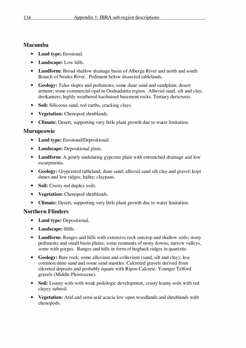
Appendix 1: IBRA sub-region descriptions
134
Macumba
• Land type: Erosional.
• Landscape: Low hills.
• Landform: Broad shallow drainage basin of Alberga River and north and south
Branch of Neales River. Pediment below dissected tablelands.
• Geology: Talus slopes and pediments; some dune sand and sandplain; desert
armour; some commercial opal in Oodnadattta region. Alluvial sand, silt and clay;
dreikanters; highly weathered kaolinised basement rocks. Tertiary duricrusts.
• Soil: Siliceous sand, red earths, cracking clays.
• Vegetation: Chenopod shrublands.
• Climate: Desert, supporting very little plant growth due to water limitation.
Murnpeowie
• Land type: Erosional/Depositional.
• Landscape: Depositional plain.
• Landform: A gently undulating gypcrete plain with entrenched drainage and low
escarpments.
• Geology: Grypcreted tableland, dune sand; alluvial sand silt clay and gravel; kopi
dunes and low ridges; halite; claypans.
• Soil: Crusty red duplex soils.
• Vegetation: Chenopod shrublands.
• Climate: Desert, supporting very little plant growth due to water limitation.
Northern Flinders
• Land type: Depositional.
• Landscape: Hills.
• Landform: Ranges and hills with extensive rock outcrop and shallow soils; stony
pediments and small basin plains; some remnants of stony downs; narrow valleys,
some with gorges. Ranges and hills in form of hogback ridges in quartzite.
• Geology: Bare rock; some alluvium and colluvium (sand, silt and clay); less
common dune sand and some sand mantles. Calcreted gravels derived from
silcreted deposits and probably equate with Ripon Calcrete. Younger Telford
gravels (Middle Pleistocene).
• Soil: Loamy soils with weak pedologic development, crusty loamy soils with red
clayey subsoil.
• Vegetation: Arid and semi-arid acacia low open woodlands and shrublands with
chenopods.
Appendix 1: IBRA sub-region descriptions
135
• Climate: Semi-arid climate that is too dry to support field crops. Soil moisture
tends to be greatest in winter.
Oodnadatta
• Land type: Erosional.
• Landscape: Plateau.
• Landform: Silcrete capped low tablelands and plains.
• Geology: Nodular, prismatic silcretes; ferricretes, calcretes, commercial quality
opal; gilgai; desert armour; hardpans; deep weathering profiles; ferruginized and
calcreted scarp exposures with pallid zones and duricrusts; porcellanitic cemented
sediments.
• Soil: Loamy soils with weak pedologic development, crusty loamy soils with red
clayey subsoils, cracking clays, brown calcareous earths.
• Vegetation: Chenopod shrublands.
• Climate: Desert, supporting very little plant growth due to water limitation.
Peake-Dennison Inlier
• Land type: Depositional.
• Landscape: Low hills.
• Landform: Bevelled low ridges of folded metamorphic rocks.
• Geology: Sand mantles over bare rock; alluvial sands, silts and clays; evaporites
(gypsum halite, some calcrete development); siliceous and ferruginous duricrusts.
• Soil: Loamy soils with weak pedologic development, crusty loamy soils with red
clayey subsoils, cracking clays, brown calcareous earths.
• Vegetation: Chenopod shrublands.
• Climate: Desert, supporting very little plant growth due to water limitation.
Pedirka
• Land type: Depositional.
• Landscape: Dunefield.
• Landform: Dune fields of large longitudinal sand dunes and interdune plains in the
north, and confused sand dune country with small claypans in the south.
• Geology: Aeolian sand, minor alluvium, colluvium and lacustrine sediments.
• Soil: Siliceous sands.
• Vegetation: Mulga (Acacia aneura) woodlands and tall shrublands with tussock
grass.
• Climate: Desert, supporting very little plant growth due to water limitation.
Simpson Desert

Appendix 1: IBRA sub-region descriptions
136
• Land type: Erosional.
• Landscape: Dunefield.
• Landform: Aeolian sandplain dominated by NNW trending seif dunes; narrow
interdune swales and corridor plains.
• Geology: Aeolian sand overlying finer sediments of alluvial or lacustrine origin.
Sands grade from red to yellow and white from N to S; white sands are more
common close to drainage ways.
• Soil: Siliceous sands.
• Vegetation: Hummock grasslands.
• Climate: Desert, supporting very little plant growth due to water limitation.
Tieyon, Finke
• Land type: Erosional / Depositional.
• Landscape: Erosional plain.
• Landform: Plains with many short and irregular shaped dunes, flat to gently
undulating sand plains with some low broad sand rises and intervening swales.
• Geology: Aeolian sand, some laterite and silcrete-capped ridges, shallow stream
valleys, calcrete mounds.
• Soil: Red earthy sands, red siliceous sands, red earths.
• Vegetation: Other tussock grasslands.
• Climate: Desert, supporting very little plant growth due to water limitation.
Warriner
• Land type: Erosional.
• Landscape: Alluvial plain.
• Landform: Plains with tracts of sand dunes; clay pans and seasonal lakes, broad
floodplains. Grypcrete remnants.
• Geology: Dune sands and sand mantles. Evaporites (gypsum, halite). Kopi dunes
and ridges. Parna and clay pans. Clayey loams, some calcareous in interdune
corridors. Alluvial sand, silt and clays in swampy lowland regions draining towards
Lake Eyre (north).
• Soil: Crusty, loamy soils with red clayey subsoils, cracking clays, brown calcareous
earths.
• Vegetation: Arid and semi-arid hummock grasslands.
• Climate: Desert, supporting very little plant growth due to water limitation.