Landcare DSS – Decision support meets interactivity

Nendel, C.*, M. Berg, K.C. Kersebaum, W. Mirschel, X. Specka, K.O. Wenkel and R. Wieland

Leibniz-Centre for Agricultural Landscape Research (ZALF), Institute of Landscape Systems Analysis, Eberswalder Straße 84, 15374 Müncheberg, Germany.

Email: nendel@zalf.de

Abstract

The Landcare decision support system (DSS) was developed to provide data and simulation models to have stakeholders informed about the likely impact of climate change on regional agriculture in Germany. The core facility of the DSS is a Google Maps®-featured Zooming User Interface in which the user can define the area of interest. Depending on the user’s choice different simulation models are offered, each of which is designed to predict specified agro-ecological variables on the selected scale. At the regional level, simulation models of intermediate complexity (REMICs) can be chosen, which apply mainly statistical or empirical approaches. At the plot scale, the dynamic, process-based simulation model MONICA can be run, simulating a range of variables for selected climate scenarios. A Farm Economy Coefficient Generator uses MONICA results to calculate farm-level accountancy figures. In addition, the climate change information section visualises regionalised data of different climate scenarios and regionalisation methods, ranging from temperature trend and rainfall pattern analyses to phenological clocks. The DSS structure is optimised for processing speed and facilitates an interactive dialogue using intuitive mechanisms for comparing simulation results.

19th International Congress on Modelling and Simulation, Perth, Australia, 12–16 December 2011 http://mssanz.org.au/modsim2011

1244

Nendel et al., Landcare DSS – Decision support meets interactivity

1. INTRODUCTION

Dissemination of scientific results and current knowledge has become a major issue in science and politics and public funding of large research projects without a clear dissemination strategy has become almost impossible. Sometimes, the dissemination pathway itself becomes the issue of research. A good dissemination strategy involves the possible stakeholders already at the definition stage of the research and continuous communication with them increases the acceptance of the result after the research phase has terminated. This applies especially for DSSs which are developed as tools to provide scientific knowledge to the user to broaden the basis of which he or she makes decisions.

Computer- or software-based decision support can be implemented in various ways. If there is a small finite set of known questions to be answered, an implementation strategy which favours custom-build static user interface elements and pre-calculated model-results is feasible and probably the best way to build a DSS. During the development of the Landcare DSS user workshops were carried out to define a general set of problems and requests, to which a computer-based DSS was considered a helpful tool. The participants were national-scale stakeholders, regional authorities or companies (e.g. insurances, energy suppliers) and farmers who were worried about the resilience of their currently used crop rotations against changing climate conditions in the coming twenty or thirty years. This mixture of scales and requirements demanded an implementation strategy for a DSS different to the one described above. Every scale has its own set of models, its users pose different kinds of questions and there is no defined boundary between the scales. Our solution to marshal the manifold possibilities was to create an open DSS framework in which only few restrictions narrow the user, but guide him while he seeks knowledge to support the pending decisions.

2. THE DECISION SUPPORT SYSTEM’S COMPONENTS

2.1. The spatial concept

Leaving the definition of the spatial context for the simulations to the user, the spatial concept of the DSS needs to account for not violating the model’s application ranges at different scales. Three types of models are available in the DSS, working on the national, the regional and on the plot scale. Depending on the user’s area selection using the ZUI, only those models are offered for exercise that are eligible for the respective scale. The number of grid cells included in the area selection that limits the application of specific models is defined by the run-time of the model, in a way that the time for running the model does not exceed the maximum acceptable response time (MART). As a rule of thumb, plot-scale models will not be offered for an application area of more than 15 × 15 grid cells, while REMICS are limited to areas smaller than approximately 1 million grid cells. For larger areas only national scale models can be applied. However, in the current version no on-line model run will be executed on the national scale. Instead, pre-run model results will be displayed. The way the spatial concept was designed assures that the user will never have to wait more than approximately 30 seconds for the system’s response (provided a sufficiently fast internet connection and computer system), allowing interactive use of the DSS by comparing different scenarios side-by side in a what-if game.

2.2. The climate data information desk

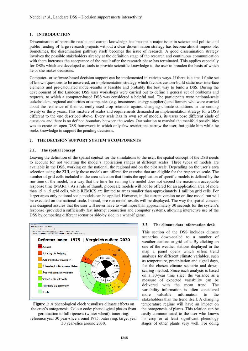
This section of the DSS includes climate scenarios down-scaled to a number of weather stations or grid cells. By clicking on one of the weather stations displayed in the map a panel opens which offers trend analyses for different climate variables, such as temperature, precipitation and signal days, for the chosen climate scenario and down-scaling method. Since each analysis is based on a 30-year time slice, the variance as a measure of expected variability can be delivered with the mean trend. The variability information is often considered more valuable information to the stakeholders than the trend itself. A changing temperature regime will have an impact on the ontogenesis of plants. This relation can be easily communicated to the user who knows his crop or at least significant phenology stages of other plants very well. For doing

Figure 1: A phenological clock visualises climate effects on the crop’s ontogenesis. Colour code: phenological phases from

germination to full ripeness (winter wheat); inner ring: reference year 30 year-slice around 1975, outer ring: target year

30 year-slice around 2030.

1245

Nendel et al., Landcare DSS – Decision support meets interactivity

this, phenological clocks are included in the panel, which allow for visualising the expected impact of climate scenarios on the different phases of the crop’ development (Figure 1). The clocks are driven by simple temperature sum algorithms.

2.3. The model base

A range of simulation models is put to the user’s disposal as soon as an area is selected using the ZUI. On the plot level, the MONICA model (Nendel et al. 2011), a dynamic process-based agro-ecosystem simulation model developed for Central European conditions, is available. Using MONICA requires the definition of a farm with a crop rotation. Standard management settings are provided by default, but can be changed by the user if desired. A Farm Economy Coefficient Generator (FECG) comes with MONICA to compute basic farm accountancy figures using MONICA’s yield simulations and standard or user-defined cost items. On the regional level, a number of REMICS is ready to use, assessing yields, deep percolation for groundwater recharge, irrigation demand, grassland productivity, erosion and other variables of interest, under future climate conditions. Further models can be added to the DSS, making the platform highly flexible for the use in different geographical environments. Currently, the DSS is being equipped for the use in the rainforest conversion zone in Mato Grosso, Brazil.

2.4. Landcare DSS interaction philosophy and general workflow

The DSS was designed as an interactive and dynamic system which enables the user to explore the defined problem space himself and meet very few restrictions while doing so. However, certain guidance features and shortcuts to open already identified pathways to problem solutions need to be provided to speed up the dialogue. In general, the user first defines a region of interest, as most of his assumed questions are connected to a specific area. The location of this area already determines most of the input parameters for the available models. The choice of the area also determines, which models can be applied, since models can only run in regions where all the required input parameters are available, else the creation of a model instance will be denied. If a selected region is eligible for a model application, a model instance for the selected region will be created and the user can use the available means to change input parameters or run the model instance with the defaults. In order to explore the problem space the user can run multiple models at the same region, run the same model at different time slices or adjust other input parameters, usually upon interpretation of previous results. In the end the user should be able to draw conclusions from the complete set of model results. It is important to note that the Landcare DSS does not interpret results or data by itself, even though in some situations common sense guidance is being applied. E.g. at the local scale some models will, by default, always run the present time slice (1991-2020) in addition to the selected, in order to put the results of the future scenario in the context of today’s situation. The means to compare different results depend on the kind of model result. For grid-based single variable results the DSS offers the basic operations one would expect (difference, merge and average of two grids). In the case of multi-value results, comparison of two model runs is just visual and specifically designed towards the ability to distinguish changes between model runs easily instead of receiving the exact quantity of a change.

Searching for a climate adaption strategy at the local scale, a farmer will be defining a small area amongst his own fields (e.g. a field with representative or problematic soil conditions). In a second step the farm type needs to be defined, using pre-defined sizes, market types, management styles, etc. A status quo run (representing today) establishes a base for an immediate plausibility check and for further examinations. If the status quo results are acceptable a second run under assumed future climate will show changes in yield, accountancy, irrigation water demand, nitrogen leaching etc. Further runs can be carried out in a game-like manner; making use of the DSS supported adaption measures. Visualisation tools help to keep track of the many results available and where changes in the adaption strategies induce significant impacts. In the end, the user has to develop a workflow which fits his/her style of thinking.

The current version of the DSS offers little support to chain models together and run them in a batch mode. However, there are models which are explicitly linked to each other (for example MONICA and the FECG at the local scale or most of the REMICS using the LANUVER land use distribution algorithm to calculate the spatial distribution of crops in a region), but this integration is currently hard-coded into the model’s DSS specific parts.

2.5. The simulation control

All models currently available in the Landcare DSS are written in C/C++ and are directly compiled into the DSS. Still care has been taken to keep them as separate as possible from the core DSS runtime, either to be able to easily run them standalone for scientific needs or to decouple them in a second step and make them run-time loadable as plug-ins. In the age of cloud-computing, multi-core and multi-processor machines it is necessary to utilise as much parallelisation potential as possible. For this reason, every model is equipped with an associated DSS interface, which embeds it into the DSS runtime and creates an environment to support as much parallel

1246

Nendel et al., Landcare DSS – Decision support meets interactivity

execution as possible. Every model is applied in a set of multiple runs, which may be due to the necessity to run (i) multiple realisations of a climate scenario in order to catch all aspects of the prospected future climate, (ii) 30 years in a time slice to create information on climate impact variability or (iii) multiple runs per crop rotation in order to get consistent results for every crop in every year (e.g. in a tripartite crop rotation the model runs three times with a one-year offset so that every crop is exposed to the complete set of climate data). This process can be easily parallelised, although the potential varies with the model and the task that is being accomplished.

In general the DSS will spawn one thread per model instance controlling overall execution and use the facilities of Qt-Concurrent (Qt, 2011) to run a model in a map-reduce fashion. There is a potential for further advanced parallelisation (e.g. running grid based models cells-by-cell), but this involves larger code refactoring and increasingly tradeoffs between ease of implementation, sequential execution speed on slower machines, and resource consumption.

2.6. The relational and spatial databases

Data management in the Landcare DSS is done in a number of SQL-databases as well as ASCII-grid files. An important part of the DSS is the associated MySQL climate database which contains all available climate simulation data and is situated on a public server. Three other databases contain the data for the models. They are usually just used locally and can either reside in a MySQL or a SQLITE database. Spatial data are stored in ASCII-grid files, mostly in a resolution of 100m × 100m. Upon start of the DSS they will be cached for efficiency reasons in HDF5 files aggregated by covered region. In this way it’s also very easy to extend the DSS to cover other regions. As long as no re-parameterisation of the models has to be done it is sufficient to copy new ASCII-grid files into the according directories of the DSS and on the next start the DSS can serve new areas. This process could be even further simplified and lifted to a run-time operation, but then parameterisation becomes the limiting factor which makes live updates a challenge.

2.7. The visualisation tool

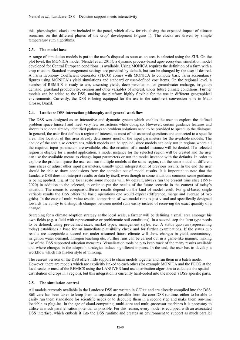
All models on the national, regional and local scale present themselves to the user with the same interface directly embedded into the ZUI. The creation of an instance of a selected model is always indicated by a largely translucent rectangle around the selected region. This rectangle region can be moved around by dragging a handle displaying the name of the model at the top. The inside of the model instance region (MIR) is reserved for the models outputs; while to the bottom edge of the MIR maps of directly manipulable input parameters for the model instance are attached (e.g. time slice, crop rotation, climate scenario; Figure 2).

Figure 2: A grid-based result of regional evapotranspiration. The result map and its surrounding model instance region (MIR) are stacked on a Google Maps® background to keep the spatial context. Attached to the

MIR, input variables maps and output statistics are displayed.

1247

Nendel et al., Landcare DSS – Decision support meets interactivity

In the current version the DSS support two kinds of outputs, grid based results and result panels for models yielding many separate single variables. Grids will in general be displayed as map overlay of the basic topographic map or satellite image provided by Google Maps® in order to keep some context for the user (Figure 2). If a model returns multiple result grids, they either get stacked upon each other or all result grids can be distributed in a flat rectangular grid. The first supports a space efficient positioning being inherently modal, while the latter can display multiple grids at once, thus offering an alternative modeless view. At the right side of these grid based results the user will usually find three additional diagrams. The two upper diagrams (a box plot and a histogram) show the spatial distribution of the grid while the lower diagram, if applicable, shows the temporal distribution of the spatial average of the result grid. This information is considered very important for the user to get a feeling for the heterogeneity in space and of climate-induced variations in time.

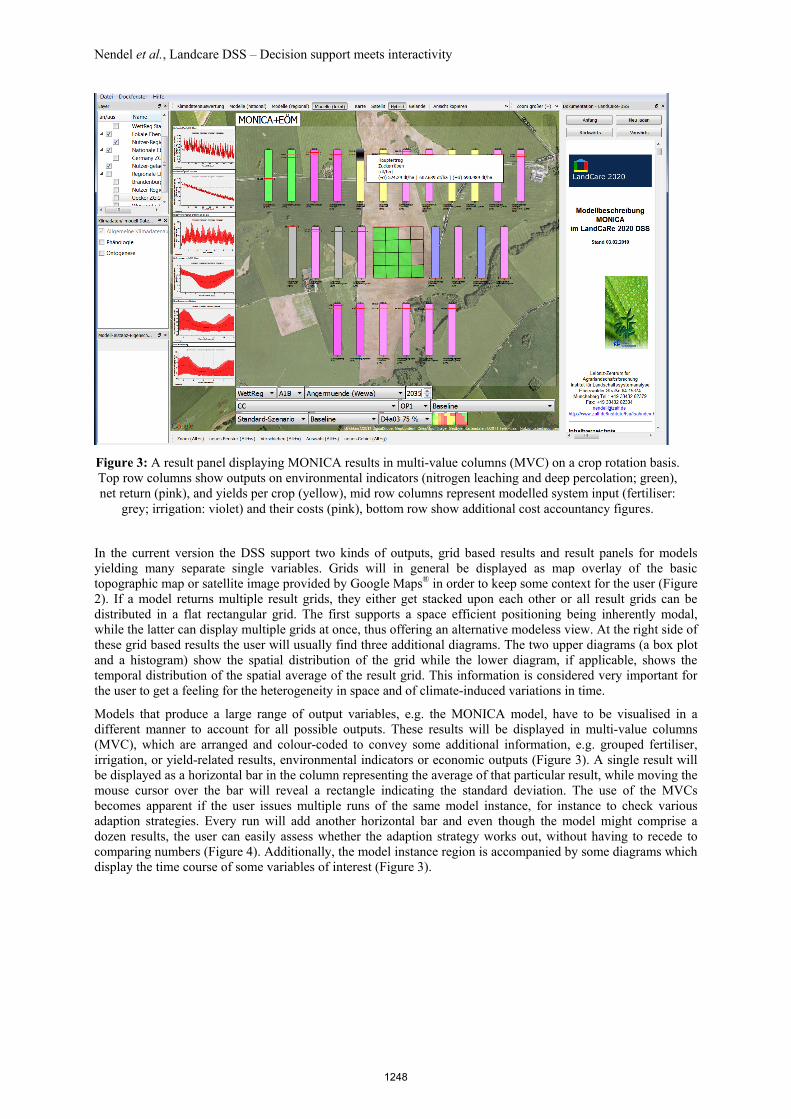
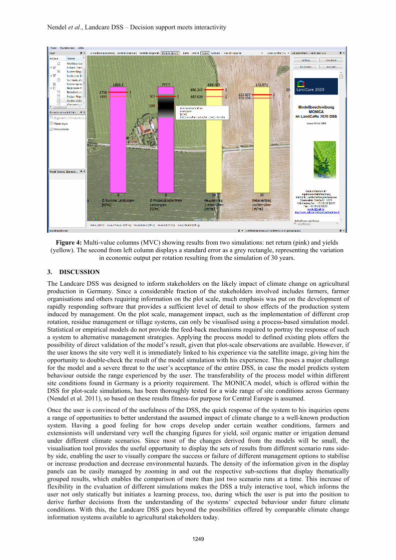
Models that produce a large range of output variables, e.g. the MONICA model, have to be visualised in a different manner to account for all possible outputs. These results will be displayed in multi-value columns (MVC), which are arranged and colour-coded to convey some additional information, e.g. grouped fertiliser, irrigation, or yield-related results, environmental indicators or economic outputs (Figure 3). A single result will be displayed as a horizontal bar in the column representing the average of that particular result, while moving the mouse cursor over the bar will reveal a rectangle indicating the standard deviation. The use of the MVCs becomes apparent if the user issues multiple runs of the same model instance, for instance to check various adaption strategies. Every run will add another horizontal bar and even though the model might comprise a dozen results, the user can easily assess whether the adaption strategy works out, without having to recede to comparing numbers (Figure 4). Additionally, the model instance region is accompanied by some diagrams which display the time course of some variables of interest (Figure 3).

Figure 3: A result panel displaying MONICA results in multi-value columns (MVC) on a crop rotation basis. Top row columns show outputs on environmental indicators (nitrogen leaching and deep percolation; green), net return (pink), and yields per crop (yellow), mid row columns represent modelled system input (fertiliser:

grey; irrigation: violet) and their costs (pink), bottom row show additional cost accountancy figures.

1248

Nendel et al., Landcare DSS – Decision support meets interactivity

3. DISCUSSION

The Landcare DSS was designed to inform stakeholders on the likely impact of climate change on agricultural production in Germany. Since a considerable fraction of the stakeholders involved includes farmers, farmer organisations and others requiring information on the plot scale, much emphasis was put on the development of rapidly responding software that provides a sufficient level of detail to show effects of the production system induced by management. On the plot scale, management impact, such as the implementation of different crop rotation, residue management or tillage systems, can only be visualised using a process-based simulation model. Statistical or empirical models do not provide the feed-back mechanisms required to portray the response of such a system to alternative management strategies. Applying the process model to defined existing plots offers the possibility of direct validation of the model’s result, given that plot-scale observations are available. However, if the user knows the site very well it is immediately linked to his experience via the satellite image, giving him the opportunity to double-check the result of the model simulation with his experience. This poses a major challenge for the model and a severe threat to the user’s acceptance of the entire DSS, in case the model predicts system behaviour outside the range experienced by the user. The transferability of the process model within different site conditions found in Germany is a priority requirement. The MONICA model, which is offered within the DSS for plot-scale simulations, has been thoroughly tested for a wide range of site conditions across Germany (Nendel et al. 2011), so based on these results fitness-for purpose for Central Europe is assumed.

Once the user is convinced of the usefulness of the DSS, the quick response of the system to his inquiries opens a range of opportunities to better understand the assumed impact of climate change to a well-known production system. Having a good feeling for how crops develop under certain weather conditions, farmers and extensionists will understand very well the changing figures for yield, soil organic matter or irrigation demand under different climate scenarios. Since most of the changes derived from the models will be small, the visualisation tool provides the useful opportunity to display the sets of results from different scenario runs side-by side, enabling the user to visually compare the success or failure of different management options to stabilise or increase production and decrease environmental hazards. The density of the information given in the display panels can be easily managed by zooming in and out the respective sub-sections that display thematically grouped results, which enables the comparison of more than just two scenario runs at a time. This increase of flexibility in the evaluation of different simulations makes the DSS a truly interactive tool, which informs the user not only statically but initiates a learning process, too, during which the user is put into the position to derive further decisions from the understanding of the systems’ expected behaviour under future climate conditions. With this, the Landcare DSS goes beyond the possibilities offered by comparable climate change information systems available to agricultural stakeholders today.

Figure 4: Multi-value columns (MVC) showing results from two simulations: net return (pink) and yields (yellow). The second from left column displays a standard error as a grey rectangle, representing the variation

in economic output per rotation resulting from the simulation of 30 years.

1249

Nendel et al., Landcare DSS – Decision support meets interactivity

For stakeholders working on a regional level, the DSS is not able to support a learning process, since feed-back relations within the system can not be considered in REMICS due to their empirical nature. However, the DSS provides fine-textured information on different topics in short time. Due to the simplicity of the REMICS quick processing time is assured, enabling the simulation on a large number of grid cells in short time and thus covering much larger areas than the process models. However, the lack of feed-back on the process basis needs to be communicated to the user, putting him in the position of interpreting the results in the light of the model’s limitations. The different concepts of the process models and the REMICS may lead to deviating results when compared for smaller areas and thus may cause irritations. One example would be the prediction of yields in a future when atmospheric CO2 levels are expected to rise in a strongly non-linear manner. The statistical yield prediction model YIELDSTAT, offered to the user on the regional scale, does consider the impact of a predicted CO2 rise in terms of an exponential trend added to the calculated yield. However, it is not able to consider the feed-back of improved water use efficiency to crop growth, which may lead to another yield increase or a lesser yield decrease, depending on the site conditions. A context-related help menu provides this additional information to the user. However, this is no guarantee that the help text is inquired so the danger of losing confidence in the system is high also for the model incompatibility over scales.

4. CONCLUSION

The Landcare DSS provides a number of novelties, which, in combination, increase the possibilities for climate change impact assessment considerably. The most important feature is surely the speed-optimised modelling software which allows for interactive gaming. Being able to design model runs on the basis of own needs, execute them and immediately compare them side-by-side puts the user into a good position to understand what scientist expect for the future of agricultural production under a changing climate. The possibilities of considering own farm specifications for the simulations makes the what-if analysis even more valuable for the stakeholder, even though the opportunity to compare the simulation results with own experience of today poses also a risk for the acceptance of the DSS by the user in case the model fails. In the end may the user’s learning process initiated by observing how the production system reacts under different stresses be the true success of the DSS.

ACKNOWLEDGMENTS

The development of the Landcare DSS was funded by the German Federal Ministry of Education and Research (BMBF) within the klimazwei research programme (Landcare2020, 01LS05109).

REFERENCES

Nendel, C., Berg, M., Kersebaum, K. C., Mirschel, W., Specka, X., Wegehenkel, M., Wenkel, K. O., and Wieland, R. (2011). The MONICA model: Testing predictability for crop growth, soil moisture and nitrogen dynamics. Ecological Modelling 222, 1614-1625.

Qt (2011). http://qt.nokia.com/.

1250