Embed Size (px)
Citation preview
Landau and Van Kampen Spectra inDiscrete Kinetic Plasma Systems
Vasil Bratanov
Master Thesis
Physics Department
LMU Munich
Scientific Advisor: Prof. Dr. Frank Jenko
Advisor at the LMU: Prof. Dr. Hartmut Zohm
25.09.2011

Declaration of Authorship
I declare that this thesis was composed by myself and that the work contained therein ismy own, except where explicitly stated otherwise in the text.
Vasil Bratanov
July 13, 2012

iv

Acknowledgements
First and foremost I would like to express my gratitude to my supervisor Prof. Dr. FrankJenko for his support and guidance that helped me to understand the framework of KineticTheory and made my work possible. I am extremely thankful both to him and Prof. Dr.Hartmut Zohm for their patience and valuable remarks during the process of writing mythesis, and for giving me the opportunity to write my Master thesis at the Max-Plank-Institut fur Plasmaphysik, Garching. Sincere thanks are given also to David Hatch, Ph.D.for the many useful discussions regarding the physics behind the mathematical models, formaking a comparison with GENE possible, and helping me improve my English. I wouldalso like to thank Dr. Stephan Brunner for the discussions, his introductory notes aboutthe slab ITG model and examples for MATLAB routines. I am also grateful to Prof. Dr.Semjon Wugalter, whose lectures provided useful insights into the topic of operator theory.Further, I would like to express my gratitude to the German Academic Exchange Service(DAAD) for its financial support during my studies.

vi

Contents
1 Introduction 11.1 Plasma physics and its relation to nuclear fusion . . . . . . . . . . . . . . . 11.2 Importance of Landau damping . . . . . . . . . . . . . . . . . . . . . . . . 31.3 Structure of the thesis . . . . . . . . . . . . . . . . . . . . . . . . . . . . . 4
2 Theoretical model of Langmuir waves in a collisionless plasma 72.1 Approximative results . . . . . . . . . . . . . . . . . . . . . . . . . . . . . 102.2 Landau approach . . . . . . . . . . . . . . . . . . . . . . . . . . . . . . . . 132.3 Van Kampen approach . . . . . . . . . . . . . . . . . . . . . . . . . . . . . 19
3 Mathematical considerations 25
4 Numerical description of Langmuir waves 354.1 Collisionless case . . . . . . . . . . . . . . . . . . . . . . . . . . . . . . . . 35
4.1.1 Maxwellian background . . . . . . . . . . . . . . . . . . . . . . . . 354.1.2 ‘Bump-on-tail’ instability . . . . . . . . . . . . . . . . . . . . . . . . 49
4.2 Introducing collision operators . . . . . . . . . . . . . . . . . . . . . . . . . 554.2.1 Krook model . . . . . . . . . . . . . . . . . . . . . . . . . . . . . . 554.2.2 Lenard-Bernstein model . . . . . . . . . . . . . . . . . . . . . . . . 56
5 Extension to ion temperature gradient (ITG) modes 735.1 The slab ITG model . . . . . . . . . . . . . . . . . . . . . . . . . . . . . . 735.2 Numerical description of collisionless ITG modes . . . . . . . . . . . . . . . 825.3 Collisional ITG modes . . . . . . . . . . . . . . . . . . . . . . . . . . . . . 88
6 Summary and conclusions 93
A Relations involving the plasma dispersion function Z 95
B Employed MATLAB codes 99

viii CONTENTS
Chapter 1
Introduction
1.1 Plasma physics and its relation to nuclear fusion
More than 99% of the matter in the Universe that can be observed directly exists as plasma,to which one often refers as the fourth state of matter. Its large abundance and the greatvariety of phenomena that occur in plasmas make the study of this state of matter animportant part of physics. Nowadays, the interest in plasma physics research is also drivenby more pragmatic reasons, namely the need for a powerful, compact, and environmentallysafe source of energy that has also practically inexhaustible fuel reserves. The only powersource known to mankind that has the potential to fulfil these conditions is nuclear fusion.This is the same process to which stars owe their energy production. The fundamentalphysics behind fusion reactions became clear already in the first half of the 20th century,and since the 1950s, scientists have been making a great effort to produce energy fromfusion in a controlled way on Earth. For fusion reactions to happen, the distance betweenthe two nuclei should be small enough such that the short-ranged strong nuclear forcedominates and the nuclei merge. However, all atomic nuclei are positively charged andrepel each other via the Coulomb force. One way to overcome these repelling forces is toheat the plasma. This increases the average kinetic energy of the particles and allows themto come closer to each other and thus enhances the probability for a quantum mechanicaltunnel effect that makes fusion possible. The approach that has made the greatest progresswith respect to a net energy gain from fusion reactions is magnetic confinement. In suchmachines, hot and dilute plasma is confined via a strong magnetic field that forces thecharged particles in the plasma to gyrate rapidly around the magnetic field lines. Thisgyromotion considerably reduces the particle transport perpendicular to the field lines andmakes interactions between plasma particles and the containing vessel infrequent such thatplasma temperatures of the order of 108K are possible. Because of this effect the optimalcontaining vessel for a magnetically confined plasma is such that at every point of theboundary the magnetic field lines are roughly tangent to the wall of the vessel. For a non-vanishing continuous vector field (e.g., a magnetic field), this condition cannot be fulfilledon a sphere (Hairy Ball Theorem due to Poincare) but it can be fulfilled for a toroidal
2 1. Introduction
surface. Therefore, in the field of nuclear fusion based on magnetic confinement, one usespredominantly Tokamaks or Stellarators, both of which have topologically the same shape,namely that of a torus.In the beginning of magnetic confinement fusion research it was thought that particles (aswell as energy and momentum) are transported across the nested toroidal magnetic sur-faces, formed by the field lines, due to collisions. When a collision between two gyratingparticles occurs, the particles can ‘jump’ to different field lines inducing cross-field trans-port. However, after a thorough mathematical analysis of such processes, it became clearthat the corresponding diffusivities are too small and cannot explain the shorter energyconfinement time observed in experiments. With the advance of fusion research, anothereffect was discovered that affects this collision-induced transport. In the twisted magneticfield of a Tokamak, the plasma particles move along complicated trajectories called ‘bananaorbits’ that can lead them rapidly from the inner to the outer part of the torus where onlyfew collisions can distort their orbit such that they do not return back in the inner part ofthe plasma. In total, this effect, called ‘neoclassical transport’, results in an outward energytransport and thus cooling the plasma which is an undesirable effect for fusion machines.The neoclassical transport expresses itself in enhancing the total transport coefficient and,therefore, decreasing the energy confinement time. However, the corresponding correctioncan be computed, and it still cannot explain the experimental results. The residual effectwas called ‘anomalous transport’, and represents one of the biggest hurdles on the way toharnessing nuclear fusion.In order to understand the reason for the anomalous transport, one first looked at fluid-likemodels of the plasma. In typical fusion machines, there are enormous density and temper-ature differences over the plasma volume. For instance, the temperature in the plasma coreis of the order of 108K, such that the conditions necessary for the nuclei to fuse are met.On the other hand, the materials which the containing vessel is made of impose an upperlimit on the energy flux that is tolerable. This leads to the fact that the outer plasmalayers have a temperature of the order of 104K. The consequences of such a limitation arethat in fusion plasmas there exist immense temperature gradients, that are of the order of108K/m. Analogous considerations for the density show that its gradient is also enormous.From fluid theory, it is known that in situations where large gradients of temperature anddensity are present, turbulent flows arise that form eddies in the plasma. These eddiesmix the fluid and, therefore, work against the gradients. The total effect of the turbulenceresults in a rapid energy transport from hotter to colder areas of the plasma. After nearlytwo decades of research in that area, it is widely agreed upon in the fusion community thatturbulence is the cause for the anomalous transport. This discovery showed that a goodunderstanding of the fundamental features of turbulence is needed in order to improve thepredictability of the behaviour of magnetized plasmas.An essential question in this context is how exactly turbulent flows arise. Strictly speaking,there exist stationary solutions for the plasma with large gradients. However, in the realworld, such a state of the plasma cannot be realized exactly. There will always be somedeviations, to which we shall refer as perturbations, of the realized state from the one thatis desired. If even an arbitrarily small perturbation of the initial condition grows steadily
1.2 Importance of Landau damping 3
in the linear approximation for some set of parameters, then this is called an instability.It is physically clear that such an instability cannot continue to grow indefinitely and hasto be saturated via nonlinear effects. According to our current understanding, such insta-bilities give rise to the turbulent flows observed. Therefore, understanding the formationand saturation of unstable modes is of great importance for the study of turbulence andits influence on the particle and energy transport in hot plasmas.Although turbulence is a notion of fluid theory, it can be influenced by kinetic effects be-cause they can cause instabilities or additional damping of the modes that determine theturbulent behaviour. Therefore, a study of kinetic effects is often needed for a thoroughunderstanding of the origin and development of turbulent flows. In this work, we are goingto focus on one of the well known and widely studied kinetic effects, namely Landau damp-ing. The simple linear models we shall use will allow us to avoid unnecessary mathematicalcomplications and concentrate on gaining physical insights that can then be used to betterunderstand the results of nonlinear numerical simulations.
1.2 Importance of Landau damping
Since the subject of this work is the Landau damping of plasma waves, it will be beneficialto focus our attention on its importance in plasma physics and fusion research. We shallshow that in the case of electrostatic perturbations of a Maxwellian background, there areno unstable (i.e., steadily growing in time) solutions. However, as we will see in this work,this is not always the case. In some models and for some sets of parameters, this simplelinear approach can lead to waves that grow with time. This is called an instability. Suchinstabilities are of great importance in fusion research since they are the main obstaclefor plasma confinement. Properties of the unstable solution, like growth rate and wavenumber, are essential because they contain the information for the time scales on whichthe instability has to be taken into account and the spatial scales on which it occurs. Asin conventional fluid mechanics, the instabilities are those effects that start and drive theturbulence. It appears also that turbulence is the major hurdle in magnetic confinementdevices that prevents achievement of large energy confinement times. Strictly speaking,discovering an unstable solution of the equations means that linear theory is not validany more, since in the framework of the linear approximation, every instability can growindefinitely, and thus at some point the approximation made by neglecting terms quadraticin the perturbations no longer applies. The real physical picture in such cases is that theinstabilities are saturated at some point, i.e., the energy that is injected into the perturbedsystem equals the energy that is dissipated. Nonlinear effects, however, can rarely betreated analytically. In such cases a numerical approach is often the only possible way toproceed. Computer simulations of plasma turbulence show that many modes which aredamped in the framework of linear theory, are excited by nonlinear effects. These dampedmodes can then couple to the unstable modes via nonlinear effects and thus facilitate satu-ration. Although linear theory is too simplified to describe the behaviour of a real plasma,it is often used to easily gain physical insights into the model. For instance, from computer

4 1. Introduction
simulations it is known that the nonlinear frequency spectrum peaks at the position of thelinear instability.From the point of view of conventional fluid theory, energy is usually injected on largescales (i.e., small wave numbers) and then dissipated on small scales (corresponding tolarge k) via viscosity (Kolmogorov cascade) [10]. Although it was thought for decades thatthis is also the case in plasmas, recent findings show that this is not the complete picture[25], [24], [28], [27]. In plasmas, a great amount of energy dissipation appears at the samespatial scales as the energy injection which means that the most important nonlinear cou-pling is that between damped and unstable modes that have similar k. This importantfeature of energy dissipation in plasmas resembles the physical picture of Landau damping,since for this phenomenon at the same wave number there exist many damped and unstablemodes that have different frequencies. This is one of the indications that Landau dampingplays an important role in the saturation of plasma turbulence. However, the connectionbetween these two effects has yet to be solidified, and a necessary step in this direction isa thorough study of the linear Landau damping also in the Van Kampen picture, investi-gating important aspects of this phenomenon that can then be qualitatively recognized innonlinear simulations.
1.3 Structure of the thesis
This thesis is organised as follows. In chapter 2, we describe the theoretical backgroundof Langmuir waves, and then study a well known kinetic effect, called ‘Landau damping’,which damps the wave amplitude exponentially for large times. The first section presentsthe physical picture of this effect via a simplified calculation which, however, preserves themost prominent feature of the Langmuir waves, namely that they are damped away. In thenext two parts of the second chapter we describe two different approaches for solving theproblem that are more mathematical in nature. The first method is due to Landau (1946)who solved the initial value problem and discovered the damping effect. After that, VanKampen (1955) found the eigenmodes of the equation which have real frequencies. Sincedamped waves have a complex frequencies, at this point confusion often arises and thisissue is clarified at the end of the second subsection.In chapter 3, we present our approach for finding the Van Kampen spectrum that is basedon operator theory. This new method improves our understanding of the problem andshows that some standard references (e.g., [13]) regarding Landau damping actually donot give completely correct results about the general conditions on which the presence andthe form of the Van Kampen spectrum depend.Chapter 4 deals with the numerical description of Langmuir waves and is divided into twosections. In the first part, we neglect collisions and reproduce some of the known analyticalresults. Here, also a short subsection is dedicated to the ‘bump-on-tail’ instability. Incor-porating collisions into the system via different collision operators is the topic of the secondsection, where we test if a discretization scheme in velocity space reproduces the analytical
1.3 Structure of the thesis 5
results stated in [18], [26] and [16], namely that the collisionless Van Kampen spectrum isaltered profoundly when collisions are introduced. Further, we investigate which part ofthe collision operator causes this abrupt change.In chapter 5, we consider electrostatic perturbations in the slab ITG model. From theequations it is evident that all we learned in chapter 3 can be applied to the ITG system.By introducing collisions into this model, we discover the same effect as in the case ofLangmuir waves.The last chapter gives a short summery of the thesis and outlines the open issues that aregoing to be the subject of subsequent work.

6 1. Introduction
Chapter 2
Theoretical model of Langmuir wavesin a collisionless plasma
In this chapter, we will discuss a simple one-dimensional model of Langmuir waves in acollisionless plasma, and consider electron oscillations with a small amplitude with respectto a homogeneous background of immobile ions such that quasi-neutrality holds. The smallamplitude of the electron oscillations allows linearisation of the equations and thus an exactanalytic solution of the problem. In this simplified model, one should also think about thephysical correctness of neglecting collisions. From a naive physical point of view, one couldargue using a time scale argument. In a real plasma, particle collisions are always goingto be present. However, if one is interested in processes that develop on time scales thatare much smaller than the average collision time, it appears to be physically reasonable toneglect the collision operator for time intervals that are sufficiently small. Although suchan argument is at first sight adequate from a physical point of view, later on in this work wewill see that collisions are of great importance for the physical system. In mathematicalterms, the collision operator, for which we shall use an approximative one-dimensionalmodel, will turn out to be a singular perturbation to the system. Therefore, if the collisionfrequency is not exactly zero, this will alter the results profoundly, no matter how smallits value is.Let f(z, v, t) be the one-dimensional electron distribution function where v is the velocityin the z−direction. From kinetic theory, it is known that f(z, v, t) should satisfy theone-dimensional Boltzmann equation. In the case when there are no external fields, andconsidering only the electric field E(z, t) produced by f , we can write the Boltzmannequation in the form
∂f
∂t+ v
∂f
∂z− e
me
E(z, t)∂f
∂v=
(∂f
∂t
)
col
, (2.1)
where e is the absolute value of the electron charge, me is the electron mass, and the right-hand side represents the general collision operator influencing the dynamics of the system.In a collisionless model, the right-hand side of (2.1) is set to zero. The equation above isnot sufficient in order to find a solution f(z, v, t). The behaviour of a system consisting of

8 2. Theoretical model of Langmuir waves in a collisionless plasma
charged particles is determined by Maxwell’s equations that are necessary to solve (2.1).Since we have neglected the influence of magnetic fields, we are left only with the Poissonequation, and in one dimension it reads
∂E(z, t)
∂z=ρ(z, t)
ε0
. (2.2)
Now, the only remaining step is to express the charge density ρ via the particle distributionfunction f(z, v, t). For this reason, we first represent f as
f(z, v, t) = f0(v) + f1(z, v, t), (2.3)
where f0(v) is the equilibrium distribution function of the electrons and f1 is the deviationfrom this equilibrium. This splitting is always possible and there is yet no approximationmade with regard to the distribution function. f0 depends only on v because the ionbackground is homogeneous (no z dependence), and the definition of equilibrium impliesno time independence. The whole dynamics of the system (in space as well as in time)comes from the perturbation f1. The electron density is by definition the integral off(z, v, t) over velocity space. Since we have split the distribution function, we can, withoutany loss of generality, also split the density as n(z, t) = n0 +n1(z, t), where these two termsare defined as
n0 :=
+∞∫
−∞
f0(v)dv ; n1(z, t) :=
+∞∫
−∞
f1(z, v, t)dv. (2.4)
These definitions are useful because there is a direct connection between the charge densityand n1. In order to see this, one should recall that in this model the ions (that have thecharge +e) are immobile, so they are always in equilibrium, and because of quasineutrality,the particle density of ions and electrons must be the same: nions = n0. This means that
ρ(z, t) = e(nions − nel(z, t)) = e(n0 − (n0 + n1(z, t))) = −e+∞∫
−∞
f1(z, v, t)dv. (2.5)
Thus, recalling (2.2), one notes that the electric field is produced by f1 and depends on itlinearly. Now we go back to (2.1) and rewrite it in a slightly different way using (2.3):
∂f1
∂t+ v
∂f1
∂z− e
me
E(z, t)∂f0
∂v− e
me
E(z, t)∂f1
∂v=
(∂f
∂t
)
col
. (2.6)
The last term on the left-hand side includes a product between E and f1. Assuming that theperturbation f1 is very small with respect to the equilibrium distribution f0, we can neglectthis term because it is of the order of f 2
1 . Performing this linearisation procedure andneglecting the collision operator yields the so-called linearised Vlasov equation. Togetherwith the Poisson equation, this gives us a self-consistent system of one differential and oneintegral equation

9
∂f1
∂t+ v
∂f1
∂z− e
me
E(z, t)∂f0
∂v= 0 (2.7)
∂E(z, t)
∂z= − e
ε0
+∞∫
−∞
f1(z, v, t)dv. (2.8)
Since we have a numerical approach in mind, it is convenient to normalize the terms inthis system of equations in such a way that the new quantities have no physical dimension.In order to do this, we consider length and time scales which are typical for the system.In our simple model of an unmagnetized homogeneous plasma, the typical length is theDebye length λD, and the typical time during which considerable changes of the systemoccur is the inverse of the electron plasma frequency ωpe. In SI units they are given by
λD =
√ε0kBT0
n0e2; ωpe =
√n0e2
meε0
(2.9)
where kB is the Boltzmann constant, ε0 the dielectric constant of the vacuum, T0 and n0
are the equilibrium temperature and density, respectively, which are defined via f0(v). Thevelocity will be normalized over the thermal velocity which we define via
vth :=
√kBT0
me
= λDωpe. (2.10)
Taking into account the above consideration, we introduce normalized expressions for thequantities which appear in our equations and denote them by a tilde over the usual symbol:
f1,0 :=vthn0
f1,0 ; E :=λDe
kBT0
E ; z :=z
λD; t := tωp ; v :=
v
vth. (2.11)
This gives us a system of normalized equations:
∂f1
∂t+ v
∂f1
∂z− E(z, t)
∂f0
∂v= 0 (2.12)
∂E(z, t)
∂z= −
+∞∫
−∞
f1(z, v, t)dv. (2.13)
When dealing with a homogeneous system like this, it is useful to make a Fourier trans-formation in space. We use the convention:
g(k) =1√2π
+∞∫
−∞
g(z)e−ikzdz (2.14)
10 2. Theoretical model of Langmuir waves in a collisionless plasma
where g(k) denotes the Fourier transform of g(z). Since we have already normalized z, thek-variable appearing after the transformation is automatically normalized to the inverse ofthe Debye length. This way we get
E(k, t) =
i
k
+∞∫
−∞
f1(k, v, t)dv. (2.15)
Substituting this expression for the Fourier transform of the electric field in the differentialequation for f1 leads to
i∂f1(k, v, t)
∂t= kv
f1(k, v, t)− 1
k
∂f0
∂v
+∞∫
−∞
f1(k, v, t)dv. (2.16)
2.1 Approximative results
Before we approach the problem of solving (2.16) in a mathematically consistent way, it isuseful to consider a simplified situation in which a damping effect arises. We will consider asimple model inspired by [9]. This will give us important physical insights about the natureof Landau damping. Let us look at a non-relativistic particle which is subject to a knownelectric field. For convenience, we assume the electric field to be a sinusoidal wave in thez-direction and that the initial velocity of the particle has also only a z-component, i.e.,we reduce the situation to a one-dimensional problem. According to the approximationsmade, the equation of motion is
mdv
dt= qE cos(kz − ωt), (2.17)
where m and q denote the mass and the charge of the particle, respectively. Withoutany loss of generality we can take the parameter k to be positive. Assuming that theelectric field is of first order, we can treat it as a small perturbation of the zeroth ordersolution which is z(0)(t) = v0t + z0, where the subscript ‘0’ denotes the initial values ofthe corresponding quantities. The first order velocity v(1) is determined by the equation ofmotion (2.17) when we substitute in it the zeroth order solution for z(t):
mdv(1)
dt= qE cos(kz0 + kv0t− ωt). (2.18)
With the initial condition v(1)(t = 0) = 0, one arrives at the result
v(1) =qE
m
(sin(kz0 + kv0t− ωt)− sin(kz0))
kv0 − ω. (2.19)
This allows us to determine the first order solution z(1) for the particle trajectory whichreads
2.1 Approximative results 11
z(1) =
t∫
0
v(1)(t′)dt′ =qE
m
(− cos(kz0 + pt) + cos(kz0)
p2− t sin(kz0)
p
), (2.20)
where the new variable p is defined as p := kv0−ω. Using z(1)(t) in the equation of motion,we can derive the second order velocity. The ultimate goal of this calculation is to find anapproximate expression for the rate of change of the kinetic energy W of the particle. Ifwe write the velocity as v = v0 + v(1) + v(2) + ..., then up to second order we have
dW
dt= m(v0 + v(1) + v(2) + ...)
d
dt(v0 + v(1) + v(2) + ...) ≈ mv0
dv(1)
dt+mv0
dv(2)
dt+mv(1)dv
(1)
dt.
(2.21)The first order term in the above expression is proportional to the right-hand side of (2.18),which is a sine function with respect to z0. Since we want to apply the results of this modelto a plasma where particles have a variety of initial positions and velocities, we have toaverage dW/dt over all possible initial positions and velocities. If we average mv0dv
(1)/dtover z0, it gives zero. Therefore, we are left only with the second order terms. Aftercalculating the second order velocity v(2) as explained above, the explicit form of dW/dtup to second order becomes
dW
dt≈ q2E2
m
(sin(kz0 + pt)− sin(kz0)
p
)cos(kz0 + pt)−
− kv0q2E2
m
(− cos(kz0 + pt) + cos(kz0)
p2− t sin(kz0)
p
)sin(kz0 + pt). (2.22)
First, we average the above quantity over all possible initial positions. Since we have ahomogeneous plasma in mind, the average process is just an integral over z0 from −∞ to+∞, i.e., the weight function is constant and equals one. This leads to
⟨dW
dt
⟩
z0
=q2E2
2m
(−ω sin(pt)
p2+ t cos(pt) + ωt
cos(pt)
p
). (2.23)
The last step left is to average (2.23) over all possible initial velocities. However, one shouldbear in mind that not all velocities are equally probable. Therefore, the weight functionfor this averaging process is the equilibrium distribution function f0(v0) which in the newnotation is f0 = f0((p+ ω)/k), i.e.,
⟨dW
dt
⟩
z0,v0
=q2E2
2mk
+∞∫
−∞
(−ω sin(pt)
p2+ t cos(pt) + ωt
cos(pt)
p
)f0((p+ ω)/k)dp. (2.24)
One can show that the contribution to the final result from integrating the second and thethird terms tends to zero when t→∞. It is noteworthy that the first term in the integrand
12 2. Theoretical model of Langmuir waves in a collisionless plasma
has a pole at p = 0 which is integrable since sin(pt) changes its sign at this point and f0
does not. We can expand f0((p + ω)/k) in Taylor series around p = 0. Since sin(pt)/p2 isan odd function of p, it is clear that only the odd terms of the Taylor series contribute tothe integral. For a qualitatively good approximation, it is sufficient to consider only thefirst odd term. This gives
p.v.
+∞∫
−∞
f0((p+ ω)/k) sin(pt)
p2dp ≈ df0
dp
∣∣∣∣p=0
p.v.
+∞∫
−∞
sin(pt)
pdp = π
df0
dp
∣∣∣∣p=0
= πdf0(v0)
dv0
∣∣∣∣v0=ω
k
.
(2.25)
From this follows
⟨dW
dt
⟩
z0,v0
= −πq2E2
2mk
(ωk
) df0(v0)
dv0
∣∣∣∣v0=ω
k
. (2.26)
The above result shows that the sign of the averaged dW/dt depends on the derivative ofthe equilibrium distribution function with respect to velocity. A realistic f0 would be aMaxwell distribution. The derivative of this function is positive when the argument is neg-ative and vice versa. This means that the product (ω/k)(df0/dv0)|v0=ω/k is always negativeand therefore
⟨dWdt
⟩z0,v0
is always positive. Recalling that the left-hand side of (2.26) is the
rate of change of the kinetic energy of an average electron/ion in the plasma under theinfluence of a small sinusoidal electric field, one sees immediately that the plasma particlesare going to gain energy from their interaction with the electrostatic wave. Because ofenergy conservation, the wave loses energy, i.e., it is damped.Another interesting observation is that, to first order, not the whole equilibrium distribu-tion influences the exchange of energy. The derivative of f0 at the point v0 = ω/k showsthat the important particles are those that move with the same speed as the phase velocityof the wave. This is due to the fact that those particles are at rest with respect to thewave, i.e., they ‘see’ a constant electric field and, therefore, can interact with the wavemuch more effectively. The particles that are moving a little faster than the wave aredecelerated, and those moving a little slower are accelerated. Strictly speaking, one shouldconsider an infinitesimally small velocity interval of length 2dv around the point v0 = ω/k.If for positive ω, there are more electrons with initial velocity v0 ∈ [ω/k − dv, ω/k] thanthose with v0 ∈ [ω/k, ω/k+dv], the wave accelerates more particles than it decelerates and,thus, loses energy. The fact that the wave interacts most effectively with the particles thathave the same velocity as its phase velocity is the reason that Landau damping is usuallyreferred to as a resonant effect. Although the model we used in this subsection was greatlysimplified, it still allowed us to gain useful physical insights into this kinetic effect andexplains how an electrostatic wave in a plasma can be damped without collisions, which isnot what one would expect intuitively.
2.2 Landau approach 13
2.2 Landau approach
The model that we used in the previous subsection was indeed sufficient for an introductioninto the topic of Landau damping and allowed to gain of some useful physical insights, butit was not self-consistent. In this part, we are going to present a mathematically rigoroustreatment of the problem of one-dimensional plasma waves.One way to solve equation (2.16) is due to Landau [11] and involves a Laplace transformin time. This method has the advantage of easily incorporating the initial condition of thesystem which is essential for determining its time behaviour. Here we are going to presentthe same idea while using a slightly different notation in order to facilitate a comparisonwith later results. Let g(t) be a function of time. We define a one-sided Fourier transformas follows:
g(ω) =1√2π
+∞∫
0
g(t)eiωtdt . (2.27)
For functions which are absolutely integrable, this integral is well defined at least in theupper ω-plane. The inverse transformation is then given by
g(t) =1√2π
+∞+iσ∫
−∞+iσ
g(ω)e−iωtdω , (2.28)
where σ is a positive real number. Applying the transformation defined in (2.27) to equation(2.16), one arrives at
− i√2π
f1(k, v, t = 0) + ω
f1(k, v, ω) = kv
f1(k, v, ω)− 1
k
∂f0(v)
∂v
+∞∫
−∞
f1(k, v, ω)dv , (2.29)
where the first term comes from integration by parts and we have used the propertythat ω has some positive imaginary part, since this is the domain of definition of this
transformation. Solving forf1(k, v, ω) and integrating over the velocity leads to
+∞∫
−∞
f1(k, v′, ω)dv′
1− 1
k
+∞∫
−∞
1
kv − ω∂f0(v)
∂vdv
=
i√2π
+∞∫
−∞
f1(k, v, t = 0)
ω − kvdv . (2.30)
If one recalls (2.15), one sees immediately that the first integral in the equation just derived
is up to a factor of i/k the transformed (Fourier transformation in space and one-sidedFourier transformation in time) electric field. This eventually gives
14 2. Theoretical model of Langmuir waves in a collisionless plasma
E(k, ω) =
1
k√
2π
∫ +∞−∞
f1(k,v,t=0)
kv−ωdv
(1− 1
k
∫ +∞−∞
1
kv−ω∂f0(v)∂v
dv) , (2.31)
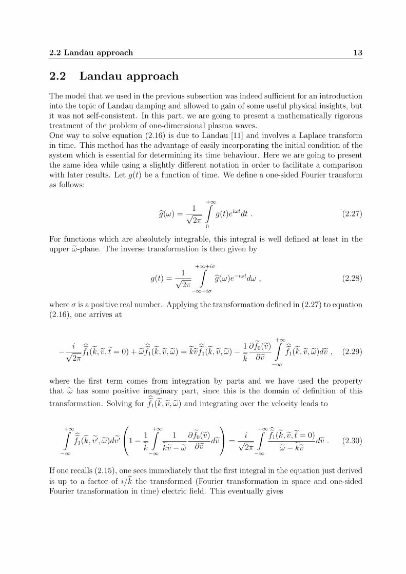
and this expression is defined in the upper half of the complex ω-plane. Since k is just areal parameter (that, without loss of generality, can be considered to be positive), thereare no poles to be encountered while performing the velocity integrals. However, in orderto perform a stability analysis of our system, we need to make sense of the integrals in(2.31) for ω in the whole complex plane, i.e., we have to continue them analytically. Sucha continuation will also help us to determine the long time behaviour of the electric field.When ω has a positive imaginary part, one can do the velocity integrals in (2.31) along thereal velocity axis, Figure 2.1 a. However, when ω approaches the real axis and crosses it,the value of the integrals will jump by 2π which means that keeping the integration alongthe real v-axis does not lead to a continuous function on the ω-plane. Therefore, in orderto have an analytic continuation, one should deform the integration contour in such a waythat the pole does not cross it. For real frequencies there is a pole on the integration path.In order to have an analytic continuation in this case, we have to deform the contour ofintegration such that the pole of the integrand at v = ω/k does not lie on the integrationpath. One way to realise this, which also satisfies causality, is to make an infinitesimalsemi-circle around the pole from below as shown in Figure 2.1 b. For Im(ω) < 0 we could,strictly speaking, perform the velocity integrals in (2.31) without any problem, since theintegrand has no poles. However, this would not be an analytical continuation of thevelocity integral. Therefore, the right contour in this case also encircles the pole as shownin Figure 2.1 c. We will refer to this way of deforming the integration contour in velocityspace as the ‘Landau prescription’. Now, when the transformed electric field is defined
in the whole complex ω-plane (except at the points where 1 − 1
k
∫ +∞−∞
1
kv−ω∂f0(v)∂v
dv = 0),
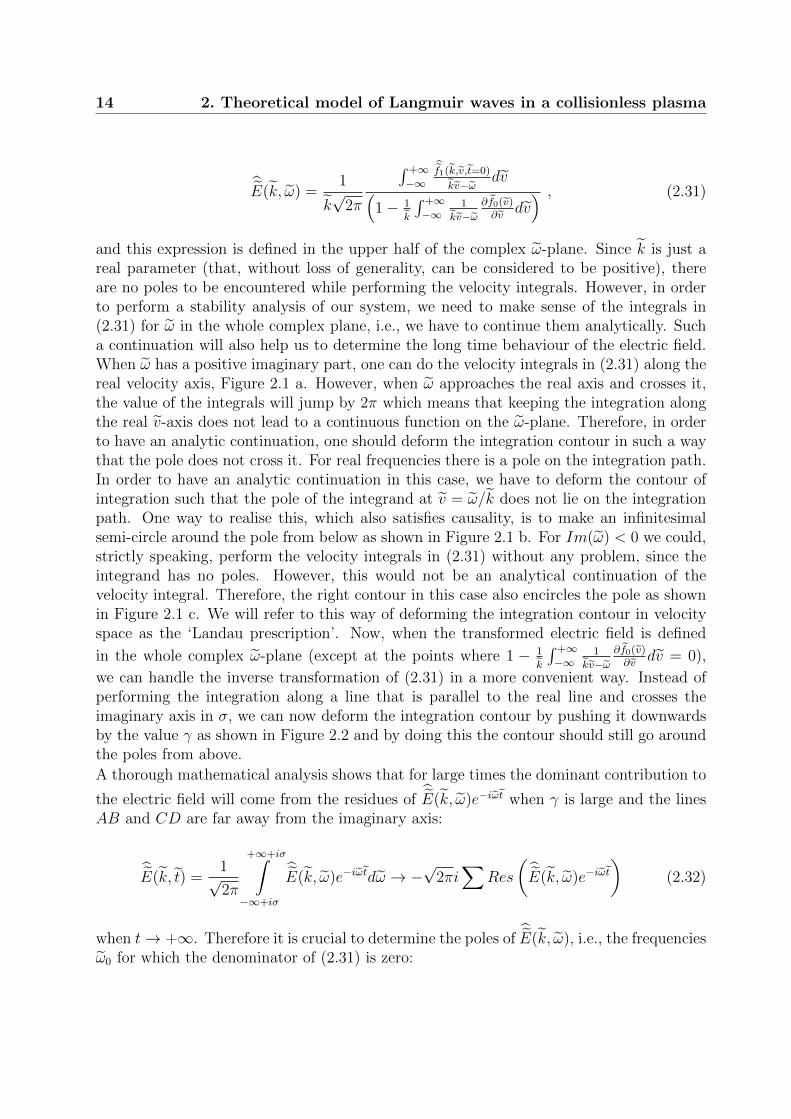
we can handle the inverse transformation of (2.31) in a more convenient way. Instead ofperforming the integration along a line that is parallel to the real line and crosses theimaginary axis in σ, we can now deform the integration contour by pushing it downwardsby the value γ as shown in Figure 2.2 and by doing this the contour should still go aroundthe poles from above.
A thorough mathematical analysis shows that for large times the dominant contribution to
the electric field will come from the residues ofE(k, ω)e−iωt when γ is large and the lines
AB and CD are far away from the imaginary axis:
E(k, t) =
1√2π
+∞+iσ∫
−∞+iσ
E(k, ω)e−iωtdω → −
√2πi∑
Res
(E(k, ω)e−iωt
)(2.32)
when t→ +∞. Therefore it is crucial to determine the poles ofE(k, ω), i.e., the frequencies
ω0 for which the denominator of (2.31) is zero:

2.2 Landau approach 15
Im( ) / thv v
Im( ) / thv v
Re( ) / thv v
Re( ) / thv v
Re( ) / thv v
Im( ) / thv v
k
k
k
)a
)b
)c
Figure 2.1: Landau contour for the analytical continuation.
1− 1
k2
∫
L
1
(v − ω0/k)
∂f0
∂vdv = 0. (2.33)
Here, the L under the integral sign means that the integral is to be calculated alongthe ‘Landau contour’ as the analytic continuation of the integrals in (2.31) requires. Inorder to evaluate this expression explicitly, we need to know the function f0(v). Since theMaxwellian distribution corresponds to the state with the maximal entropy of the system,it is physically sound to assume that the equilibrium distribution of our system is alsoMaxwellian, i.e.,
f0(v) =n0√
2πkBTi/mi
exp
(− miv
2
2kBTi
). (2.34)
Using the normalization procedure outlined in (2.11), one easily sees that
16 2. Theoretical model of Langmuir waves in a collisionless plasma
Im( ) / pe
Re( ) / pe
D
C
A
B
Figure 2.2: Path of integration for the analytic continuation of the electric field.
f0(v) =1√2π
exp
(−1
2v2
). (2.35)
With this expression, equation (2.33) turns into
1− 1√2πk2
∫
L
ve−v2/2
(v − ω0/k)dv = 0 . (2.36)
As outlined in the Appendix, the integral on the right-hand side can be expressed throughthe plasma dispersion function Z defined in [1] as:
∫
L
ve−v2/2
(v − ω0/k)dv =
√2π
(1 +
ω0√2kZ
(ω0√2k
)). (2.37)
Substituting this into (2.36) yields a dispersion relation of the form
1 + k2 +ω0√2kZ
(ω0√2k
)= 0 , (2.38)
which is much easier to work with.

2.2 Landau approach 17
Basic properties of the dispersion relation
Before we evaluate (2.38) numerically, it is useful to analytically gain some insight into
what the solutions of this equation look like. First, we define x0 := Re(ω0)/(√
2k) and
y0 := Im(ω0)/(√
2k) and then split (2.38) into real and imaginary parts:
1 + k2 + x0ReZ(x0, y0)− y0ImZ(x0, y0) = 0 (2.39)
x0ImZ(x0, y0) + y0ReZ(x0, y0) = 0. (2.40)
Concerning the symmetry properties of Z, we know [1] that ReZ(−x, y) = −ReZ(x, y)and ImZ(−x, y) = ImZ(x, y). This means that if the pair (x0, y0) is a solution of theupper system of equations, so is the pair (−x0, y0), i.e., the set of solutions of (2.38) issymmetric with respect to the imaginary ω-axis.Next, we would like to prove analytically that (2.38) has only damped solutions, i.e.,solutions that lie in the lower half of the complex ω-plane. At this point, one usually citesthe Penrose criterion. However, for a Maxwellian equilibrium distribution there is alsoa straightforward proof of the non-existence of unstable or marginal solutions. First, weinvestigate if there are solutions on the real line (i.e., with y0 = 0). In this case the lastterms in (2.39) and (2.40) equal zero, so in (2.40) we are left with
x0
√πe−x
20 = 0 ,
where we have used ImZ(x, 0) =√πe−x
2[1]. The upper equation has only one solution,
namely x0 = 0, but substituting this result in (2.39) leaves us with a left-hand side in the
form 1 + k2 that cannot equal zero, since k is real.Now we consider the possibility that x0 = 0, i.e., that there are solutions on the imaginaryaxis. In this case, (2.40) transforms into y0ReZ(0, y0) = 0, which, however, gives us nocondition, since ReZ(0, y) ≡ 0 for all y. We are thus left only with (2.39), which now reads
1 + k2 − y0ImZ(0, y0) = 0. For y > 0, we know that
yImZ(0, y) =y2
√π
+∞∫
−∞
et2
t2 + y2dt =
1√π
+∞∫
−∞
et2
1 +(ty
)2dt <1√π
+∞∫
−∞
et2
dt = 1. (2.41)
Since we have a strict inequality, we know that (for x0 = 0 and y0 > 0) the left-hand sideof (2.39) is strictly positive, so there cannot be any solutions lying on the upper part ofthe imaginary ω-axis. Although our goal is merely to prove the non-existence of unstablesolutions, for the sake of completeness, we also show that there are no solutions on thewhole imaginary axis. If x = 0 and y < 0, we have that Z(0, y) = Z∗(0, |y|) + 2i
√πey
2=
−iImZ(0, |y|) + 2i√πey
2[1]. From this it immediately follows that

18 2. Theoretical model of Langmuir waves in a collisionless plasma
k2 + 1− y0ImZ(0, y0) = k2 + 1− |y0|ImZ(0, |y0|)︸ ︷︷ ︸>0
+2√π|y0|e|y0|
2
>
> k2 + 2√π|y0|e|y0|
2
> 0. (2.42)
Since we now know that there are no solutions on the axes and that the set of solutionsis symmetric with respect to the imaginary ω-axis, it suffices to show that there are nosolutions for x0 > 0 and y0 > 0 in order to prove the non-existence of unstable solutions. Todo this, we recall the connection between the plasma dispersion function and its derivative,namely that Z ′(ξ) = −2(1+ξZ(ξ)) for all ξ [1]. Since Z is by definition an analytic function,we can write that
dZ(ξ)
dξ=∂ReZ(x, y)
∂x+ i
∂ImZ(x, y)
∂x=∂ImZ(x, y)
∂y− i∂ReZ(x, y)
∂y. (2.43)
Using these relations, one can rewrite (2.38) as
dZ(ξ)
dξ|ξ=x0+iy0=
∂ReZ(x, y0)
∂x|x=x0+i
∂ImZ(x, y0)
∂x|x=x0= 2k2. (2.44)
Since the right-hand side of the last expression is real, a necessary condition for the ex-istence of a solution is that the derivative of the imaginary part of Z with respect to xequals zero at the solution. For y > 0 ImZ(x, y) reads as follows:
ImZ(x, y) = y1√π
+∞∫
−∞
e−t2
(t− x)2 + y2dt. (2.45)
A derivation of this relation is given in the Appendix. There we also prove that the integralcommutes with a derivative with respect to x. Therefore, we can write that
∂ImZ(x, y0)
∂x|x=x0= y0
2√π
+∞∫
−∞
(t− x0)e−t2
((t− x0)2 + y20)2
dt. (2.46)
Since we look for solutions in the area {y0 > 0}⋃{x0 > 0}, the last expression equals zeroif and only if the integral part is zero, so we focus on this integral. A simple substitutionp := t− x leads to
+∞∫
−∞
(t− x0)e−t2
((t− x0)2 + y20)2
dt = −ex20+∞∫
0
pe−p2e2px0
(p2 + y20)2
+ ex20
+∞∫
0
pe−p2e−2px0
(p2 + y20)2
=
= −2e−x20
+∞∫
0
pe−p2
sinh(2px0)
(p2 + y20)2
dp. (2.47)
2.3 Van Kampen approach 19
Looking at the last integral in (2.47), it is immediately clear that for x0 > 0 the integrandis almost everywhere positive. Therefore, the partial derivative of ImZ(x, y) with respectto x is negative in the second quadrant of the complex ω-plane. By this we have provedthat there exist no unstable (and even no marginal, i.e., Imω0 = 0) solutions of (2.38).
Numerical solutions of the dispersion relation
Now we can focus on the implementation of this equation and solve it numerically. At firstsight (2.38) looks simple, but the left-hand side is a complex valued function that takesalso complex numbers as arguments, i.e., a full plot of the behaviour of this function will befour-dimensional, and thus difficult to work with. A way to simplify the problem withoutmaking any approximations is to note that (2.38) is true if and only if
∣∣∣∣1 + k2 +ω0√2kZ
(ω0√2k
)∣∣∣∣ = 0 . (2.48)
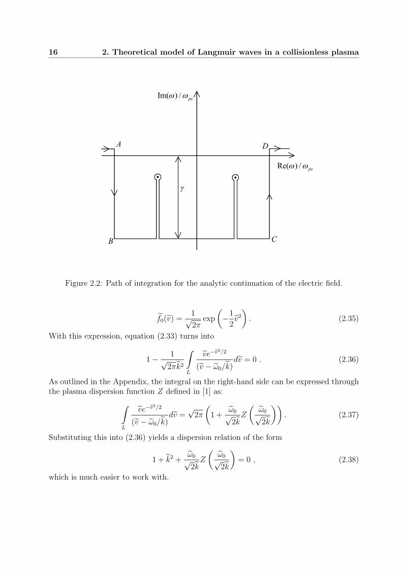
On the left-hand side we now have a function that maps C onto R, so the space of argumentsand values of this function is three-dimensional. Since also the left hand side of (2.48) is bydefinition non-negative, the solutions of this equation will be the points where the surfacedefined by this function touches the complex ω-plane. A convenient way to find those pointsis to draw a contour plot in the ω-plane for some value of the parameter k (here k = 0.5)as shown in Figure 2.3. This plot is produced using MATLAB, version R2009b, with theprogram landau.m, the code of which is shown in the Appendix. The left-hand side of(2.48) was evaluated on a quadratic grid in the ω-plane with the resolution of ∆ω = 0.001while the contours are drawn on equidistant ‘heights’ from 0 to 0.02 in steps of 0.001. Onesees that all solutions lie in the lower part of the ω-plane, which in our notation correspondsto damping, as had to be expected in this simplified model of homogeneous plasma. Sincethese solutions are the poles of (2.31), they are going to determine the long time behaviourof the electric field produced by the perturbation f1(z, v, t), i.e., the electric field will decayexponentially and for t→∞ only the least damped solutions (closest to the real axis) willbe important. This phenomenon is usually called ‘Landau damping’. One also sees thesymmetry of the solutions with respect to the imaginary axis which we derived analytically.
2.3 Van Kampen approach
In the literature, there is also another approach for solving (2.16) which is due to VanKampen [12]. With this method, one looks for stationary solutions. Here, we are not goingto follow all the steps described in [12]. Instead, we merely outline the ideas that lead tothe result of Van Kampen and set the scene for the numerical computations to follow. Inorder to solve (2.16), we do a Fourier transformation of the equation in time,

20 2. Theoretical model of Langmuir waves in a collisionless plasma
−3 −2 −1 0 1 2 3−2.5
−2
−1.5
−1
−0.5
0
0.5
Re(ω)/ωpe
Im(ω
)/ωpe
Figure 2.3: Landau solutions for k = 0.5.
f1(k, v, ω) =
1√2π
+∞∫
−∞
f1(k, v, t)eiωtdt . (2.49)
This definition is similar to (2.27)1, which will make the comparison between the resultsof the two approaches easier. Applying this transformation on (2.16) gives
ωf1(k, v, ω) = kv
f1(k, v, ω)− 1
k
∂f0
∂v
+∞∫
−∞
f1(k, v, ω)dv. (2.50)
This is an integral equation forf1(k, v, ω), whose general solution is, as Van Kampen
showed,
f1,V (k, v, ω) = p.v.
(1
k
∂f0(v)/∂v
kv − ω
)+ δ(kv− ω)
k − p.v.
+∞∫
−∞
1
kv′ − ω∂f0(v′)
∂v′dv′
, (2.51)
1In this convention a negative imaginary part of ω also corresponds to damping.
2.3 Van Kampen approach 21
where δ denotes the Dirac delta function. One can verify that this solves (2.50) by ex-plicitly substituting (2.51) into the equation. A subtlety one should account for is thatxδ(x) = 0, which follows from the theory of distributions. p.v. in front of the integral in(2.51) indicates that one should take the Cauchy principal value of the integral. There isalso the abbreviation p.v. in front of the first expression in (2.51). It merely denotes that,
if one happens to integrate this expression over k, v or ω, the Cauchy principal value ofthe integral should be taken, but it does not influence algebraic manipulations. Clearly,for every real ω there is a solution of (2.50) (a Case-Van Kampen mode), so the spectrumof frequencies, that the Van Kampen approach gives, is the whole real axis.The Van Kampen modes are singular functions that do not represent a physically meaning-ful perturbation. Therefore, to study the time dependence of a physical initial perturbation,one should consider a superposition of uncountably infinitely many Van Kampen modesand then take their inverse Fourier transform with respect to time, i.e.,
f1(k, v, t) =
+∞∫
−∞
q(k, ω)f1,V (k, v, ω) e−iωt dω , (2.52)
where the function q(k, ω) is chosen such thatf1 fulfils the conditions discussed in more
detail in chapter 3. After substituting (2.51) into the last expression, two integrals emerge.The first one reads
p.v.
+∞∫
−∞
q(k, ω) e−iωt
kv − ωdω = −e−ikvt p.v.
+∞∫
−∞
q(k, kv − x) eixt
xdx . (2.53)
The integral on the right-hand side looks rather general, but for a large class of functionsq one can show that it does not depend on time. We assume that q(k, kv − x) has nosingularities along the x-axis. In the case of an initial value problem, one considers theevolution of a perturbation whose value is prescribed at t = 0. Since we are interestedin its behaviour for t > 0, we take an analytical continuation of q in the upper half ofthe complex plane and also demand that q does not increase faster than some polynomialof |x| for |x| → ∞. In this case, the integrands in (2.53) have at most one pole alongthe integration path. For evaluating the principal value integral we close the contour ofintegration by a semi-circle CR of radius R in the upper half of the complex plane. Thepole at x = 0 is circumvented from above by a semi-circle of an infinitesimal radius. Now,one can write
∮q(k, kv − x) eixt
xdx = p.v.
+∞∫
−∞
q(k, kv − x) eixt
xdx− iπRes
(q(k, kv − x) eixt
x
)∣∣∣x=0
+
+ limR→∞
∫
CR
q(k, kv − x) eixt
xdx . (2.54)

22 2. Theoretical model of Langmuir waves in a collisionless plasma
Since the integrand on the left-hand side is taken to be analytic in the upper half of thecomplex plane, the integration along the closed path we have chosen gives zero. The semi-circle CR is parametrized as follows: x = R cosφ + iR sinφ ; φ ∈ [0, π]. Recalling that, ifq goes to infinity for large R, it is not faster than some power of R, it immediately followsthat the contribution from the semi-circle is zero, i.e.,
∫
CR
q(k, kv − x) eixt
xdx = i
π∫
0
q(k, kv − x) eiR cosφt e−R sinφt dφ ∼ RNe−R → 0 for R→ +∞ .
(2.55)
The second integral that emerges after a substitution of (2.51) into (2.52) involves adelta function and is therefore trivial. Taking this into account, as well as the fact that
Res(q(k, kv − x)eixt/x)|x=0 = q(k, kv), the entire expression forf1(k, v, t) reads
f1(k, v, t) = q(k, kv)
(−iπ 1
k
∂f0(v)
∂v+ k−
−p.v.+∞∫
−∞
1
k(v′ − v)
∂f0(v′)
∂v′dv′
e−ikvt =: g(k, v) e−ikvt . (2.56)
This shows explicitly that the entire time dependence off1(k, v, t) (and therefore also of
f1(z, v, t)) is in the exponential factor e−ikvt. Since k, v and t are real variables, it is clearthat this factor represents just oscillating behaviour in time with no growth or decay. Wealso make another observation in order to facilitate future comparison. Let us view k asa fixed parameter and look at this exponential factor at a given time t0. Now we studythe behaviour of the real part2 of the exponential factor in velocity space. This is a cosinefunction with kvt0 as an argument. Since the values of the cosine repeat when its argumentequals n2π where n ∈ N, the same structure in velocity space will repeat after an interval of∆v = 2π
kt0. If we make the same analysis at a later time, say t = t1 > t0, the corresponding
∆v will be even smaller, i.e., the oscillation off1 with respect to velocity becomes more
and more rapid with time. This allows us to make a statement about the Fourier transform
in space of the electric field which by definition is an integral off1(k, v, t) over velocity,
i.e.,
E(k, t) =
i
k
+∞∫
−∞
g(k, v) e−ikvt dv → 0 as t→ +∞ . (2.57)
2The same conclusions also apply to the imaginary part.

2.3 Van Kampen approach 23
The above result concerning the behaviour of the electric field in the limit for large t is aconsequence of the Riemann-Lebesgue lemma. In order that this lemma can be appliedin the present case, the function g(k, v) should be absolutely integrable with respect to
velocity. We choose q in such a way that this is true. Bearing in mind that k, v and t arereal, it can easily be seen that
+∞∫
−∞
|g(k, v)| dv =
+∞∫
−∞
| f1(k, v, ω) eikvt| dv =
+∞∫
−∞
| f1(k, v, ω)| dv . (2.58)
In the next chapter, we will discuss in more detail the functional space to whichf1 should
belong in order that the above integral is finite and that the same applies also to all itsvelocity moments. This inevitably imposes similar conditions on q. Since in the VanKampen approach there are only modes with real frequencies, (2.57) might look surprisingat first sight. This time limit becomes intuitive if one views the integral over velocityin (2.57) as the surface enclosed under the integrand. If g is a continuous function withrespect to velocity, which is a reasonable physical condition, the integrand becomes moreoscillatory when time evolves and the variation of g during one period gets smaller, so thecancellation between the areas above and below the real axis becomes more accurate. Thelimit process in (2.57) is what one usually identifies with ‘linear Landau damping’ and isreproduced also by the Van Kampen method.At first sight, it might look like the two approaches presented in this and the previoussubsection, both solving (2.16) in a mathematically consistent way, lead to different results.However, this is not the case. It is important to note that Landau solved the initial valueproblem for the electric field which, in Fourier space, is proportional the 0th velocitymoment of the distribution function, and there are uncountably infinitely many differentdistribution functions that give the same electric field after integration. On the other hand,Van Kampen solved (2.16) for the distribution function. Therefore, his result in terms ofeigenfrequencies should not be directly compared to the Landau solutions. One first hasto integrate over velocity in order to gain the electric field and, as we saw in (2.57), thiselectric field is damped also when using the Van Kampen solutions. In the literature, theintegration over velocity is usually referred to as ‘phase mixing’. This is due to the factthat for every fixed velocity, the integrand in (2.57) represents a harmonic oscillator. Thevelocity integration is the mathematical analogue to mixing uncountably infinitely manysuch oscillators where each of them has a different frequency.

24 2. Theoretical model of Langmuir waves in a collisionless plasma
Chapter 3
Mathematical considerations
One can view (2.50) as an integral equation determiningf1. Solutions for this equation are
the Case-Van Kampen modes which involve a delta function in velocity space. However,in this subsection we view (2.50) as an eigenvalue equation where the right-hand side is
a linear operator acting on the Fourier transform of the perturbation f1. It should beclarified that these are merely two different perspectives and the solutions that arise inthis way should be the same if one defines the operator appropriately. Since we are onlyinterested in the eigenvalues of this operator, we are going to suppress for simplicity all
unnecessary symbols accompanyingf1 and also all arguments except v. The linear operator
A, whose eigenvalues we want to find, is defined through its action on the perturbation ofthe electron distribution function, i.e., the right hand side of (2.50):
(Af) (v) := kvf(v) + ψ(v)
+∞∫
−∞
f(v′)dv′ (3.1)
where for the sake of generality we have written ψ(v) in front of the integral. In the
case of Langmuir waves, ψ(v) = − 1k∂f0(v)∂v
. For a linear operator like A, we need not onlya linear prescription like (3.1) that defines the action on a given function, but also thefunctional domain on which this operator is defined. The function f is the perturbation ofthe distribution function. From a physical point of view, one can impose on it the conditionthat all its velocity moments are finite, i.e.,
∣∣∣∣∣∣
+∞∫
−∞
vnf(v)dv
∣∣∣∣∣∣<∞ for every n ∈ N0. (3.2)
This condition is fulfilled for every function in the Schwartz space S which, said figuratively,is defined as the functional space of all rapidly falling functions of a real argument thatare infinitely many times continuously differentiable. However, for simplicity we take as adomain of definition of A, i.e. D(A), the space

26 3. Mathematical considerations
H := {f(v) ∈ L2|vf(v) ∈ L2}. (3.3)
As we will show in this chapter, for the functions in H one can only say with certainty thattheir 0th velocity moment is finite, i.e., the operator A be well defined. This is sufficient,since in this work we are not going to encounter any higher moments of f . It is alsonoteworthy that the Schwartz space is dense in H, i.e, S is a subspace of H and for everygiven function f ∈ H there exist a sequence of functions {gn} ∈ S such that ‖gn− f‖ → 0.In other words, every function in H can be approximated with an arbitrary accuracy witha function in S. If we have defined the domain of A as S, then this would not have changedthe important results of this chapter. It is useful to choose as a domain of A a Hilbertspace. Neither S nor H are Hilbert spaces when equipped with the usual scalar productin L2. However, with a new scalar product 〈·, ·〉H , defined as
〈f, g〉H :=
+∞∫
−∞
f(v)(1 + |v|)2g(v)dv, (3.4)
where f, g ∈ H, the space H can be turned into a Hilbert space.In order that the operator A is well defined, the right-hand side of (3.1) (more preciselythe integral) has to be finite for any f in the domain of A. This can be easily verified asfollows:
∣∣∣∣∣∣
+∞∫
−∞
f(v)dv
∣∣∣∣∣∣=
∣∣∣∣∣∣
+∞∫
−∞
f(v)(1 + |v|)1 + |v| dv
∣∣∣∣∣∣=
∣∣∣∣⟨
(1 + |v|)f(v),1
1 + |v|
⟩
L2
∣∣∣∣ ≤
≤ ‖(1 + |v|)f(v)‖L2 · ‖ 1
1 + |v|‖L2
︸ ︷︷ ︸=√
2
=√
2‖f(v) + |v|f(v)‖L2 ≤
≤√
2‖f(v)‖L2 +√
2‖|v|f(v)‖L2 <∞. (3.5)
In the course of this work, we will see that the function ψ(v) will always be a Gauss functiontimes some polynomial which means that for the purpose of this work ψ ∈ H. In this case,the range of A is L2, i.e.,
A : H → L2. (3.6)
So far, we have only made some plausible definitions in order to express a physical prob-lem in a more mathematical fashion, but we have not gained any further understanding.However, this more rigorous formulation of the problem will soon allow us to utilize sometheorems from operator theory in order to make a more precise statement about the spec-trum of A. First, one should note that A is a sum of two parts, A0 and C, which we defineas

27
(A0f)(v) := kvf(v) ; (Cf)(v) := ψ(v)
+∞∫
−∞
f(v′)dv′. (3.7)
The domain of both operators we set as H. It is immediately seen that A0 is (up tothe real parameter k which is qualitatively not important) just a multiplication operatorby v. A0 is equivalent to the position operator in quantum mechanics which has beenthoroughly studied. Defined as a map from H onto L2, as in this case, it is known to beself-adjoint and to have only an essential1 spectrum that consists of the entire real axis,i.e., σess(A) = R. Now we focus our attention on the second term, namely on C. From thedefinition of C, it is clear that this operator maps every function f ∈ H to a function thatis proportional to ψ where only the proportionality factor (in this case an integral over fwhich, for ease of notation, we will denote as γf ) depends on f . In other words, C mapsan infinite dimensional Hilbert space onto a finite dimensional space which is a subspace ofL2. Another important property of C is that it is a bounded operator which can be easilyseen as follows. First, note that
‖Cf‖L2 =√〈Cf,Cf〉L2 = |γf | · ‖ψ‖L2 . (3.8)
Recalling (3.5), we have
|γf | ≤√
2‖(1 + |v|)f(v)‖L2 =√
2‖f‖H (3.9)
which leads to
‖Cf‖L2
‖f‖H=|γf | · ‖ψ‖L2
‖f‖H≤√
2‖f‖H · ‖ψ‖L2
‖f‖H=√
2‖ψ‖L2 <∞. (3.10)
Since C is a bounded operator with a finite dimensional range, it follows that C is com-pact. We can now use this knowledge in order to apply a theorem due to Weyl [6, p. 113,Corollary 2] which in terms of our notation states the following:
Let A0 be a self-adjoint operator and let C be a relative compact perturbation of A0. Then:a) A = A0 + C defined with D(A) = D(A0) is a closed operator.b) If C is symmetric, A is self-adjoint.c) σess(A) = σess(A0).
Thus, A also has an essential spectrum consisting of the entire real axis. The mathematicaldomain of definition for A, which we chose, reproduces the physical result. However, theaforementioned theorem does not state that this is the whole spectrum of A. It is possible,and here this is also the case, as we shall see, that the perturbation C has created someisolated eigenvalues. In order to show this, we have to determine the complete spectrum
1In this chapter we will often make use of the term ‘essential’ regarding the description of some part ofa spectrum. In physics one usually calls this ‘continuous’ spectrum.

28 3. Mathematical considerations
of the operator. It is noteworthy that, in our case, the operator C is indeed compact, butit is not symmetric with respect to the scalar products 〈·, ·〉H or 〈·, ·〉L2 . Therefore, theoperator A is not self-adjoint.A convenient way to find the eigenvalues ω of A would be first to find the resolvent ofA − ω and then to search for its poles. (More precisely, we should not speak abouteigenvalues but rather about points of the spectrum, which is defined as the complementof the resolvent set. It can be, for example, that an operator has a non-empty spectrum butno eigenvalues in the mathematical sense of this word. However, from a physical point ofview it is convenient to call every, in general complex, number ω that satisfies the equationAfω = ωfω an eigenvalue of A although this is an abuse of mathematical ideas.) One wayto do that is to take the equation
((A− ω) f) (v) = h(v), (3.11)
where h(v) is given and to try to solve it for f(v). Using the definition of A, we find that
f(v) =h(v)
kv − ω − γfψ(v)
kv − ω . (3.12)
Integrating (3.12) over velocity space gives us an expression for γf which consists only ofknown functions. Substituting this expression into (3.12), we arrive at
f(v) =h(v)
kv − ω −ψ(v)
kv − ω ·1
1 +∫ +∞−∞
ψ(v′)kv′−ωdv
′
+∞∫
−∞
h(v′)
kv′ − ωdv′. (3.13)
One could view the right-hand side of (3.13) also as a linear operator acting on h(v), namelyas
f(v) = (R(ω,A)h) (v), (3.14)
where the operator R(ω,A) is the resolvent of A− ω and is given explicitly by
R(ω,A) =1
kv − ω −ψ(v)
kv − ω1(
1 +∫ +∞−∞
ψ(v′)kv′−ωdv
′)
+∞∫
−∞
dv′
kv′ − ω . (3.15)
Since k and v are real numbers, it is immediately clear that R(ω,A) has a pole for everyreal number. This is the essential spectrum of A, which corresponds to the solution ofVan Kampen and also emerges in our mathematical analysis of A. However, from (3.15)one easily sees that this is not the entire spectrum, since R(A − ω,A) also has poles forfrequencies which satisfy the relation
1 +
+∞∫
−∞
ψ(v)
kv − ωdv = 0 (3.16)
29
and which we will denote by ω0. It is noteworthy that the pole in the integrand in theabove expression makes it ambiguous. For the integral to have a definite value, it has tobe specified how this pole is treated, and later on we will see that different treatments canyield completely different results.One can easily verify by substitution that the eigenfunctions fω(v) of the operator A havethe form
fω(v) = − ψ(v)
kv − ω + kδ(kv − ω)
1 + p.v.
+∞∫
−∞
ψ(v)
kv − ωdv
. (3.17)
In the case of a Maxwellian equilibrium distribution, this gives the same result as (2.51).Another observation that is straightforward to make is that, if ψ(v) is an odd function,then the spectrum is symmetric with respect to zero, and for the corresponding eigen-functions we have that f−ω(v) = fω(−v). At first sight, it might look disturbing that theeigenfunctions (3.17) do not belong to the functional space H which we used as a domain ofA. However, since the functions fω(v) are integrable, we can technically apply A on them.Actually, this is a common situation in mathematics. For instance, the Laplace operatoris usually defined as a quadratic form on the first Sobolev space, which is also dense in L2,but its eigenfunctions are the plane waves that do not belong to L2. Nevertheless, they areinfinitely many times continuously differentiable and the Laplace operator can, technically,be applied on them. The situation with the operator A is completely analogous. Naively,one might have expected that the eigenfunctions fω(v) involve a delta function in velocityspace. This comes from the fact that the Fourier transform with respect to velocity of theoperator A0 is proportional to the momentum operator known from quantum mechanics.The eigenfunctions of the momentum operator are the plane waves, and the inverse Fouriertransform of a plane wave is a delta function. Of course, an arbitrary operator C addedto A0 could have altered the eigenfunctions profoundly, but in our case the influence ofC on the eigenfunctions is merely change of the constant in front of the delta function(corresponding to the amplitude of the plane wave) and the addition of the first term in(3.17).
Next we would like to say something more about the solutions ω0 in the case of Langmuirwaves. For this we recall that ψ(v) = − 1
k∂f0(v)∂v
. As an equilibrium distribution functionwe take a centred normalized Maxwellian distribution which is given by
f0(v) =1√2πe−
12v2 . (3.18)
Taking this into account and introducing the new variable a0 defined as a0 := ω0/(√
2k),we arrive at the equation
1 +1√πk2
+∞∫
−∞
xe−x2
x− a0
dx = 0 (3.19)
30 3. Mathematical considerations
where the new integration variable x is related to the velocity via x = v/√
2. The problemwith this integral is that its value is ambiguous if Im(a0) = 0, since in this case there isa pole on the integration path for x = Re(a0) and the value of the integral depends onhow we treat this pole. One option, which corresponds to the solution of Van Kampen,would be to take the Cauchy principal value (denoted in this thesis by p.v. in front of theintegral). We will show in the rest of this subsection that this treatment of the pole leadsto solutions of (3.19) which are real.First, we divide a0 into real and imaginary parts as a0 = Re(a0) + iIm(a0) =: a0r + ia0i.
This allows us to split also the integral∫ +∞−∞
xe−x2
x−a0 dx, which one can view as a complexvalued function of a0, into a real and an imaginary part. Substituting this result in (3.19),gives us the following system of two equations
1 +1√πk2
p.v.
+∞∫
−∞
x(x− a0r)e−x2
(x− a0r)2 + a20i
dx = 0 (3.20)
1√πk2
a0ip.v.
+∞∫
−∞
xe−x2
(x− a0r)2 + a20i
dx = 0. (3.21)
If a0i 6= 0, the notation p.v. can, of course, be omitted, since there is no ambiguity regard-ing the value of the integral. However, we will keep it for convenience. There are threecases in which the second equation is satisfied: a0i = 0, the integral is zero, or both a0i andthe integral equal zero. Since the third case is fulfilled if and only if the other two are, itsuffices to consider only the first two cases.
Case 1: a0i = 0If this is the case, then we have only real solutions which was what we wanted to prove.
Case 2: p.v.∫ +∞−∞
xe−x2
(x−a0r)2+a20idx = 0
Substituting this relation into the first equation of system (3.20) leads to
1 +1√πk2
+∞∫
−∞
x2e−x2
(x− a0r)2 + a20i
dx = 0. (3.22)
The integral which appears in (3.22) is clearly positive, so (3.22) has no solutions (k is realby definition), i.e., the condition that determines Case 2 is never fulfilled.However, the system of equations (3.20), whose solution is by definition a0, must holdwhich means that a0i = 0, i.e., a0 ∈ R.Since we now know that (3.19) has only real solutions, we can easily show that
ω0rp.v.∫ +∞−∞
e−x2
x−ω0r/(√
2k)dx is an even function of ω0r which means that, if ω0r is a solution
of
31
− ω0r√2k
1√πp.v.
+∞∫
−∞
e−x2
x− ω0r√2k
dx = 1 + k2, (3.23)
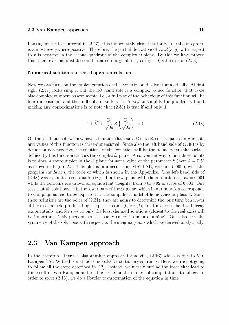
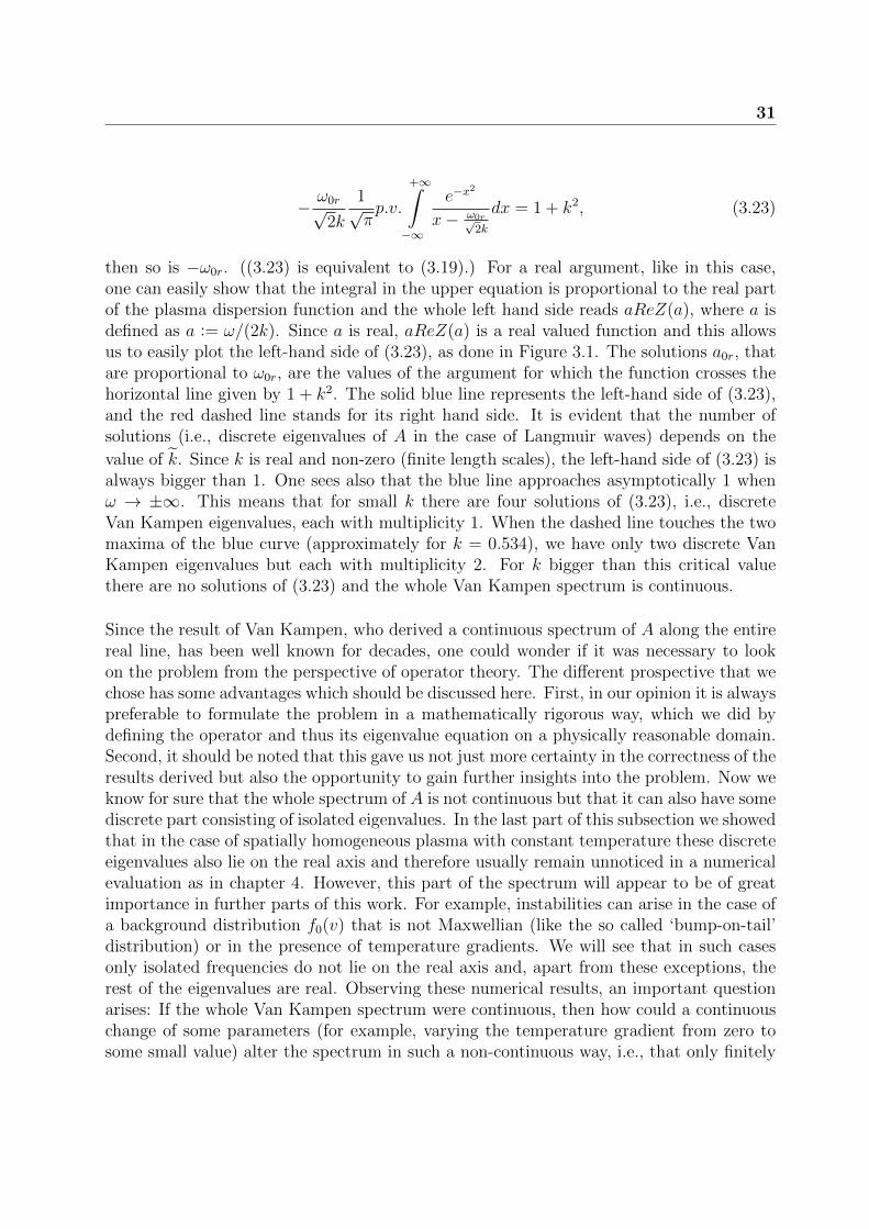
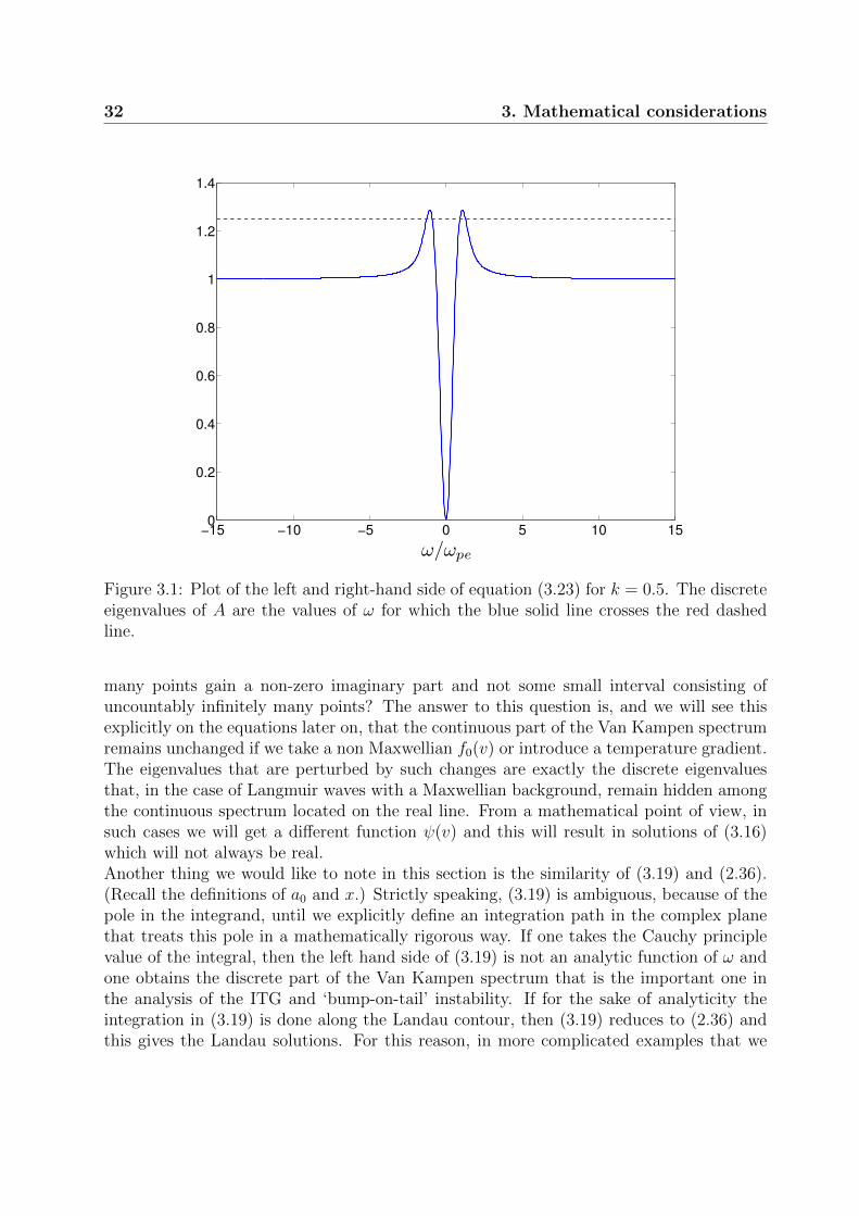
then so is −ω0r. ((3.23) is equivalent to (3.19).) For a real argument, like in this case,one can easily show that the integral in the upper equation is proportional to the real partof the plasma dispersion function and the whole left hand side reads aReZ(a), where a isdefined as a := ω/(2k). Since a is real, aReZ(a) is a real valued function and this allowsus to easily plot the left-hand side of (3.23), as done in Figure 3.1. The solutions a0r, thatare proportional to ω0r, are the values of the argument for which the function crosses thehorizontal line given by 1 + k2. The solid blue line represents the left-hand side of (3.23),and the red dashed line stands for its right hand side. It is evident that the number ofsolutions (i.e., discrete eigenvalues of A in the case of Langmuir waves) depends on the
value of k. Since k is real and non-zero (finite length scales), the left-hand side of (3.23) isalways bigger than 1. One sees also that the blue line approaches asymptotically 1 whenω → ±∞. This means that for small k there are four solutions of (3.23), i.e., discreteVan Kampen eigenvalues, each with multiplicity 1. When the dashed line touches the twomaxima of the blue curve (approximately for k = 0.534), we have only two discrete VanKampen eigenvalues but each with multiplicity 2. For k bigger than this critical valuethere are no solutions of (3.23) and the whole Van Kampen spectrum is continuous.
Since the result of Van Kampen, who derived a continuous spectrum of A along the entirereal line, has been well known for decades, one could wonder if it was necessary to lookon the problem from the perspective of operator theory. The different prospective that wechose has some advantages which should be discussed here. First, in our opinion it is alwayspreferable to formulate the problem in a mathematically rigorous way, which we did bydefining the operator and thus its eigenvalue equation on a physically reasonable domain.Second, it should be noted that this gave us not just more certainty in the correctness of theresults derived but also the opportunity to gain further insights into the problem. Now weknow for sure that the whole spectrum of A is not continuous but that it can also have somediscrete part consisting of isolated eigenvalues. In the last part of this subsection we showedthat in the case of spatially homogeneous plasma with constant temperature these discreteeigenvalues also lie on the real axis and therefore usually remain unnoticed in a numericalevaluation as in chapter 4. However, this part of the spectrum will appear to be of greatimportance in further parts of this work. For example, instabilities can arise in the case ofa background distribution f0(v) that is not Maxwellian (like the so called ‘bump-on-tail’distribution) or in the presence of temperature gradients. We will see that in such casesonly isolated frequencies do not lie on the real axis and, apart from these exceptions, therest of the eigenvalues are real. Observing these numerical results, an important questionarises: If the whole Van Kampen spectrum were continuous, then how could a continuouschange of some parameters (for example, varying the temperature gradient from zero tosome small value) alter the spectrum in such a non-continuous way, i.e., that only finitely
32 3. Mathematical considerations
−15 −10 −5 0 5 10 150
0.2
0.4
0.6
0.8
1
1.2
1.4
ω/ωpe
Figure 3.1: Plot of the left and right-hand side of equation (3.23) for k = 0.5. The discreteeigenvalues of A are the values of ω for which the blue solid line crosses the red dashedline.
many points gain a non-zero imaginary part and not some small interval consisting ofuncountably infinitely many points? The answer to this question is, and we will see thisexplicitly on the equations later on, that the continuous part of the Van Kampen spectrumremains unchanged if we take a non Maxwellian f0(v) or introduce a temperature gradient.The eigenvalues that are perturbed by such changes are exactly the discrete eigenvaluesthat, in the case of Langmuir waves with a Maxwellian background, remain hidden amongthe continuous spectrum located on the real line. From a mathematical point of view, insuch cases we will get a different function ψ(v) and this will result in solutions of (3.16)which will not always be real.Another thing we would like to note in this section is the similarity of (3.19) and (2.36).(Recall the definitions of a0 and x.) Strictly speaking, (3.19) is ambiguous, because of thepole in the integrand, until we explicitly define an integration path in the complex planethat treats this pole in a mathematically rigorous way. If one takes the Cauchy principlevalue of the integral, then the left hand side of (3.19) is not an analytic function of ω andone obtains the discrete part of the Van Kampen spectrum that is the important one inthe analysis of the ITG and ‘bump-on-tail’ instability. If for the sake of analyticity theintegration in (3.19) is done along the Landau contour, then (3.19) reduces to (2.36) andthis gives the Landau solutions. For this reason, in more complicated examples that we

33
will study, we are not going to undertake the complicated analysis of contour deformationas in section 2.2. Instead, we will derive the corresponding resolvent operator, separateits discrete part and treat the ambiguity differently (Cauchy principle value or Landauprescription) which will give us the discrete part of the Van Kampen spectrum and theLandau solutions respectively.At this point, we would like to make a few comments regarding the classic paper [13] ofCase about one-dimensional electrostatic electron oscillations in a plasma with immobileions viewed in the framework of linear theory. The notation used in this paper is similarto that which is used here, except that in [13] η(v) is what we here called ψ(v) and theeigenvalues are denoted by ν, and are related to ours via the simple formula ν = ω/k.In his paper (on page 353), Case summarizes his results by claiming that: ‘We have acontinuum of solutions for all real ν such that not simultaneously
η(νi) = 0 = λ(νi) ≡ 1 +
+∞∫
−∞
η(v)dv
v − νi.’ (3.24)
Considering the rest of the paper, most probably the Cauchy principle value of the integralin the expression above is meant. However, in this part of our work we showed that thiscannot be true. Let us take a Maxwell distribution for the form of f0(v). In this case, ηequals zero only when its argument also equals zero, so the first condition of (3.24) cannotproduce a continuous spectrum consisting of the entire real line. The second condition,involving λ, is the same as (3.16) with the Cauchy principle value prescription, and wesaw in this subsection that this expression is directly related to the real part of the plasmadispersion function, because the argument (here νi) is taken to be real. Since ReZ(x, 0)is not proportional to 1/x, λ(νi) cannot have the same value for all real νi. From this,it follows that the conditions given in (3.24) cannot reproduce the known continuous VanKampen spectrum which, as we know for certain, exists when f0 is a Maxwell distribution.There is also a more general argument for that. Our mathematical analysis showed thateven the multiplication operator A0 alone has a continuous spectrum situated on the entirereal line. We also proved, using a general mathematical theorem of Weyl, that the additionof the operator C does not change anything about the continuous spectrum of A0, since Cis compact. The function η(v), however, is present only in C. Therefore, one can concludethat presence of the continuous part of the spectrum cannot be influenced by any conditionthat involves η(v), which is the case for both conditions in (3.24). The continuous VanKampen spectrum is a remnant of the operator A0 and, therefore, has nothing to do withthe particular form of η(v).Further, we would also like to discuss the discrete part of the spectrum. In his paper, Casenotes that also discrete sets of eigenvalues can exist:“We have a discrete set of solutions for νi such that either νi is complex and
+∞∫
−∞
η(v)dv
v − νi= 1 (3.25)

34 3. Mathematical considerations
or νi is real with η(νi) = λ(νi) = 0.’As we already noted, η(v) is the same as ψ(v) in our notation, so condition (3.25) is similarto (3.16). The two conditions would have been the same if the right-hand side of (3.25)were −1 instead of 1. We think that this discrepancy is due to a typing error. However,the conditions regarding the discrete set of real eigenvalues also do not agree with ourresults. As we found, there exist isolated eigenvalues given by (3.16) where one shouldtake the Cauchy principle value of the integral. In the notation of Case, (3.16) correspondsto λ(νi) = 0. However, η(νi) = 0 does not need to be fulfilled. For example, in the caseof a Maxwell background electron distribution η(νi) = 0 is true only for νi = 0 but, as wesaw, in this case (3.16) is satisfied also for values of ω0 different from zero. By applying Aon the eigenfunction corresponding to these real non-zero eigenvalues one sees that theystill fulfil the eigenvalue equation even though η(νi) 6= 0.
Chapter 4
Numerical description of Langmuirwaves
4.1 Collisionless case
4.1.1 Maxwellian background
In the previous chapter we set the basis for a better qualitative mathematical understandingof the spectrum of the operator A. However, such a qualitative understanding is notcompletely satisfactory. Instead, we would like to have some quantitative results thatdescribe the system under consideration. Even in the collision free case, the equationsare complicated enough such that the results we are interested in cannot be expressedin a closed form using elementary functions, i.e., we cannot derive an analytic solution.Therefore, we are going to undertake a numerical approach. In subsequent parts of ourstudy, when we include also complicated collision operators, e.g., the Lenard-Bernsteincollision operator, we will have to rely almost exclusively on numerical results. In section2.2 we have already used numerics to find the solutions of (2.48). In this part we modelnumerically the Van Kampen approach. For this we are going to discretize the velocityaxis which turns the distribution function into a vector in a high but finite dimensionalspace (dimension equals the number of points in velocity space), i.e.,
v ∈ (−∞,+∞)→ {vj}j=1,2,...,N+1 =⇒ f1(k, v, ω)→ F (k, vj, ω) =: Fj, (4.1)
where Fj stands for the jth component of the vector ~F representing the Fourier transformedperturbation of the distribution function in velocity space. We shall also use a set of pointsin velocity space that is symmetric with respect to 0. The derivative of the equilibriumdistribution function with respect to v is also expressed by a vector which will be denotedby ~G:
Gj :=∂f0
∂v(vj). (4.2)

36 4. Numerical description of Langmuir waves
With this notation (2.50) becomes
ωFj = kvjFj −1
kGj ·
N+1∑
i=1
Fi∆v
︸ ︷︷ ︸↔
∫+∞−∞
f1(k,v,ω)dv
, (4.3)
where ∆v is the distance between two neighbouring points on an equidistant grid in velocityspace and the integral over velocity has been transformed into a finite sum. We want toexpress the right-hand side of (4.3) as matrix acting on the vector ~F . Mathematically,this means that we approximate the continuous operator on the right-hand side of (2.50),i.e., A, through a matrix. Naively thinking, one could expect that, if one takes more andmore points on the velocity axis, i.e., one makes the matrix bigger, then the approximationshould get better and better. This, however, is not straightforward. Since A, defined onthe Hilbert space H, is not a compact operator, we can be certain that there does not exista sequence of matrices, i.e., finite rank operators, that converges to A in the operator norm[7, p. 135, Satz 3.8 d)]. In our case this means that increasing the rank of the matrices, i.e.,making the resolution in velocity space better, does not necessarily make the numericalresults more correct. Therefore, we are going to test our numerical approximation againstsome known qualitative results which have been derived analytically. If we are able toreproduce these results, then this will give us some confidence in the methods we use.First, we make the discretisation of the velocity axis more precise. When the index j runsfrom 1 to N + 1, the velocity points will vary from −vmax to vmax, where the latter isdefined as the maximal velocity in the set and corresponds to j = N + 1. This leads to
vj = −vmax + (j − 1)∆v = −vmax +2vmaxN
(j − 1). (4.4)
According to this we have for the first term on the right-hand side in (4.3):
kvjFj = −k(vmax + ∆v)Fj + k∆vjFj (4.5)
and jFj is the jth component of the vector given by the product
1 0 0 · · · 00 2 0 · · · 00 0 3 · · · 0...
......
. . ....
0 0 0 · · · N + 1
F1
F2
F3...
FN+1
=: B · ~F . (4.6)
If we define a (N + 1)-dimensional row-vector ~b as ~b := (1, 1, 1, ..., 1), then the second termon the right in (4.3) can be rewritten as follows:
−∆v
k
{Gj
N+1∑
j=1
Fi
}= −∆v
k~G(~b · ~F
)= −∆v
k
(~G⊗~b
)· ~F . (4.7)
4.1 Collisionless case 37
This way we can rewrite (4.3) in a more convenient form, namely as a matrix eigenvalueequation:
ω ~F = M · ~F , (4.8)
where the matrix M is given by
M = −kvmax(N + 2)
NI + k∆vB − ∆v
k~G⊗~b. (4.9)
and I represents the identity matrix of rank N + 1. For a numerical evaluation we have tospecify the vector ~G. Since we want to reproduce the Van Kampen spectrum of Langmuirwaves that corresponds to the set of Landau solutions which we already derived in section2.2, we take also in this case a normalized and centred Maxwellian as an equilibriumdistribution given in (3.18). This means that
G(v) = − v√2πe−v
2/2. (4.10)
Now we can easily evaluate (4.8) by writing a simple routine in MATLAB (shown in theAppendix under the name eigenvalue.m) that diagonalizes M and plots its eigenvalues.
Such a plot for vmax = 6, k = 0.5 and 51 points in velocity space is shown in Figure 4.1,where the crosses represent the position of the calculated eigenvalues.It is evident that the program produces only real eigenvalues which is consistent with ourexpectation based on the mathematical analysis in chapter 3. The largest deviation ofan eigenvalue from the imaginary axis is of the order of 10−15. Since in this example thenumerical precision was set to double, this deviation is due to numerical ‘noise’. Anotherinteresting observation that one can make and on which we are going to elaborate furtherlater on, is that the density of the eigenvalues on the real line (inverse proportional tothe distance between two neighbouring eigenvalues) is not constant. We have plottedthis spectral density (solid blue line) in Figure 4.2 where for convenience it is normalizedthrough a multiplication by ∆v. The horizontal black dashed line represents the constantfunction of 2.A comparison with Figure 2.1 shows that the position of the two peaks coincides with theprojection of the least damped Landau solutions onto the real axis (represented here via thetwo vertical red dashed lines). In other words, the Van Kampen eigenvalues somehow sensethe presence of the most important Landau solutions. It is noteworthy that the spectraldensity has noticeable variations only in the central part of the frequency interval while forfrequencies considerably greater than the real part of the least damped Landau solution itquickly approaches the value of 2. In order to understand this behaviour and the meaningof the constant line, we recall the resolvent operator of A that is given explicitly by (3.15).
The first part of this operator is 1/(kv − ω) and it is responsible for the continuous partof the spectrum. If this were the whole resolvent operator, then in a discretized velocityspace also the continuous spectrum becomes discrete with eigenvalues that are given byωj = kvj. This leads to equidistant points that are separated by ∆ω = k∆v. In this case,

38 4. Numerical description of Langmuir waves
−4 −3 −2 −1 0 1 2 3 4−0.1
−0.08
−0.06
−0.04
−0.02
0
0.02
0.04
0.06
0.08
0.1
Re(ω)/ωpe
Im(ω
)/ωpe
vmax = 6vth ; ∆v = 0.24vth ; kλD = 0.5
Figure 4.1: Collisionless Van Kampen spectrum for k = 0.5.
the spectral density according to our definition would have been ∆v/∆ω = 1/k = 2 whichcorresponds to the black dashed line. However, the whole spectral density is not given bya constant function. From this, it follows that the non-trivial behaviour of the density ofthe eigenvalues is determined by the second part of the resolvent operator which is due tothe operator C that arises from the Poisson equation in our model. In front of the integralin the expression for C there is the derivative of the equilibrium distribution which werepresented by a Maxwell distribution centred around zero. This means that ∂f0(v)/∂vfalls rapidly when velocity increase. Since the velocity is related to the frequency byv = ω/k, this can explain why for large ω the operator C has practically no influence onthe spectral density.Another qualitative test of our numerical approach is to reproduce Landau damping. Sincedamping is a phenomenon concerning the time behaviour of the quantity in view, we willtherefore turn to equation (2.16). In order to prevent further complication of the notation,
the discretised version off1(k, v, t) is also going to be denoted by ~F . Bearing this in mind,
the discretised version of (2.16) can be written as
i∂ ~F (t)
∂t= M · ~F (t), (4.11)
which is a first order differential equation in time. Since the matrix M depends neither on

4.1 Collisionless case 39
−3 −2 −1 0 1 2 31.96
1.98
2
2.02
2.04
2.06
2.08
2.1
2.12
Re(ω)/ωpe
spectral density
vmax = 6vth ; ∆v = 0.06vth ; kλD = 0.5
Figure 4.2: Spectral density of the collisionless Van Kampen spectrum (k = 0.5).
time nor on the vector ~F , we can write the solution of this equation immediately as
~F (t) = e−iMt · ~F0, (4.12)
where ~F0 represents the value of ~F at t = 0 which is regarded as given. Equation (4.12) canbe easily implemented numerically which we have done with the program initial value.mgiven in the Appendix. Using this program (combined with distribution.m), one canproduce the plot shown in Figure 4.3. As an initial condition we have taken a normalizedGauss curve centred at 0 with the width of 2. At first sight this could be confusing sincewe have used the same function also for the equilibrium distribution. However, (4.11) islinear, so we can multiply its solution with an arbitrary number (in order to satisfy thesmallness condition that the perturbation f1 has to fulfil) and it will still be a solution.A physically more reasonable initial condition would be a shifted Gauss function with adifferent width which corresponds to a population of particles that moves with respect tothe ion background and has a different temperature than the majority of the electrons.Nevertheless, such an initial condition produces qualitatively the same result as the onewe have used in order to show the increasing oscillation of f1 with time.
One observes exactly the oscillation behaviour with respect to velocity which gets moreand more rapid when time increases as we expected, as shown in Figure 4.3.The last test of our numerical scheme is to reproduce the exact value of the damping
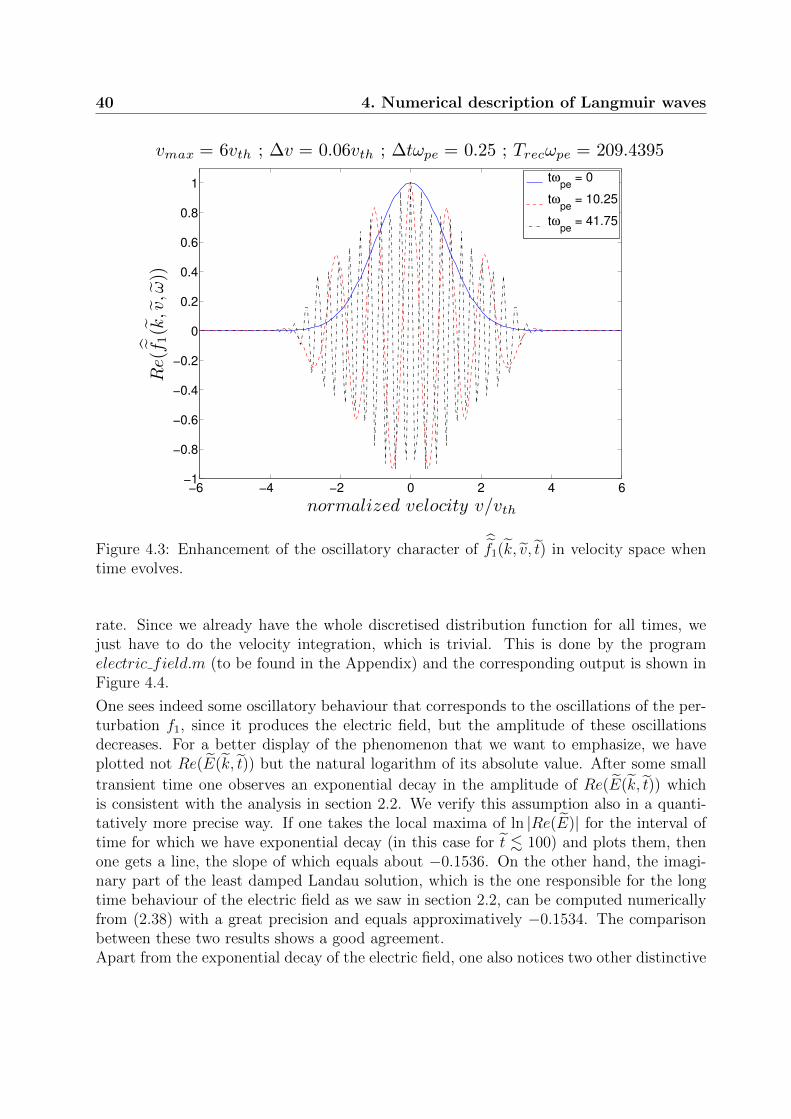
40 4. Numerical description of Langmuir waves
−6 −4 −2 0 2 4 6−1
−0.8
−0.6
−0.4
−0.2
0
0.2
0.4
0.6
0.8
1
normalized velocity v/vth
Re(
f 1(k,v,ω
))vmax = 6vth ; ∆v = 0.06vth ; ∆tωpe = 0.25 ; Trecωpe = 209.4395
tωpe
= 0
tωpe
= 10.25
tωpe
= 41.75
Figure 4.3: Enhancement of the oscillatory character off1(k, v, t) in velocity space when
time evolves.
rate. Since we already have the whole discretised distribution function for all times, wejust have to do the velocity integration, which is trivial. This is done by the programelectric field.m (to be found in the Appendix) and the corresponding output is shown inFigure 4.4.
One sees indeed some oscillatory behaviour that corresponds to the oscillations of the per-turbation f1, since it produces the electric field, but the amplitude of these oscillationsdecreases. For a better display of the phenomenon that we want to emphasize, we haveplotted not Re(E(k, t)) but the natural logarithm of its absolute value. After some small
transient time one observes an exponential decay in the amplitude of Re(E(k, t)) whichis consistent with the analysis in section 2.2. We verify this assumption also in a quanti-tatively more precise way. If one takes the local maxima of ln |Re(E)| for the interval oftime for which we have exponential decay (in this case for t . 100) and plots them, thenone gets a line, the slope of which equals about −0.1536. On the other hand, the imagi-nary part of the least damped Landau solution, which is the one responsible for the longtime behaviour of the electric field as we saw in section 2.2, can be computed numericallyfrom (2.38) with a great precision and equals approximatively −0.1534. The comparisonbetween these two results shows a good agreement.Apart from the exponential decay of the electric field, one also notices two other distinctive

4.1 Collisionless case 41
0 50 100 150 200 250 300 350 400−10
−8
−6
−4
−2
0
2
normalized time tωpe
lg|R
e( f 1(k,v,ω
))|
vmax = 6vth ; ∆v = 0.06vth ; ∆tωpe = 0.25 ; Trecωpe = 209.4395
Figure 4.4: Time dependence of the Fourier transform of the electric field.
features in Figure 4.4. First, all structures seem to repeat periodically. This is not a phys-ical effect but is due to our discretisation of velocity space. Once we have set the length ofthe velocity interval [−vmax, vmax] and the number of points it is to be represented with,the minimal distance of points ∆v is determined. This is the resolution in velocity space.If one recalls the exponential factor in (2.56), then it is clear that a non-zero ∆v leads
to finite time Trec (which we will call recurrence time) given by Trec = 2π
k∆vafter which
the phase φ can be related to the phases from previous times as φ(t) = φ(t − Trec) + 2πwhich, of course, leads to the same value of the exponent, i.e., this periodic behaviour is aconsequence of our numerical treatment and does not represent real physics, so results fort > Trec should be ignored. The other effect is what appears to be a saturation effect justbefore recurrence occurs. In a linear theory such a saturation effect does not exist and theelectric field should be damped to zero. However, every computer has a certain numericalprecision and the electric field cannot be damped under this precision which in our caseproduces the effect observed. In Figure 2.15 the numerical saturation occurs at values ofthe electric field of the order of 10−7. The reason for this is that in our program there wereobjects defined with the computer precision single. Therefore, this is also the precision ofthe end result.Now, after we have successfully tested our numerical approach, we would like to use it togain more information about the system under consideration. As we already observed in

42 4. Numerical description of Langmuir waves
Figure 4.2, the Van Kampen eigenvalues, although bound to the real axis, seem to sensethe position of the least damped Landau solutions by increasing their density just abovethese Landau roots. This hints at the importance of the Van Kampen modes that corre-spond to these eigenvalues. In the Landau approach of solving the collisionless linearisedVlasov equation one solves for the electric field E and one discovers that it is dampedexponentially. However, as we already explained, the distribution function is not damped.It just oscillates more rapidly in velocity space as time increases. It is not straightfor-ward to connect the Van Kampen modes with Landau damping, since the electric fieldis proportional to the 0th velocity moment of the distribution function and there are un-countably infinitely many distribution functions that reproduce a damped electric fieldwith a given damping rate. Therefore, we are going to use our numerical scheme to in-vestigate this matter. Since we took a finite interval on the velocity axis and discretizedit, the continuous operator A turned into a matrix and the eigenvectors of this matrix,which we will denote by ~e`, correspond to the Van Kampen modes. Every vector ~e` is afunction of velocity in the sense that every component of the (N + 1)-dimensional vectoris the value of this function at the corresponding point in velocity space. Integration ofthis function over velocity translates into the sum of all components of ~e` multiplied bythe grid resolution ∆v. As eigenvectors of the matrix M , defined in (4.9), {~e`}`=1,2,...,N+1
form a basis in the space of (N + 1)-dimensional vectors. The vectors of this basis are nor-malized by MATLAB but they are not orthogonal. In order to make the further analysismore convenient, we introduce the so called left eigenvectors ~g` of M that are defined bya similar eigenvalue equation, namely ~gT` ·M = ω`~g
T` . A well known result from Linear
Algebra is that for non-degenerate eigenvalues ~em · ~gn = 0 when n 6= m. At this point aremark has to be made. The eigenvectors are normalized to one with respect to the usualnorm of finite dimensional vectors. However, this is going to make a comparison betweenanalytical and numerical results harder. The reason for this is that this scalar product offinite dimensional vectors corresponds to the L2 scalar product of functions. The numericaleigenvectors have to represent the analytical eigenfunctions that we found and that are notsquare integrable. In the literature the eigenfunctions are, therefore, usually ‘normalized’such that their integral over velocity is one1. A possible solution of this problem is tonormalize the numerical eigenvectors such that the sum of their components is one, i.e.,that
∆vN+1∑
m=1
e`m = 1 for every ` ∈ {1, 2, ..., N + 1}. (4.13)
This can be easily done by merely rescaling every component the vector e` in the appro-priate way. A plot of one of the numerical eigenvectors (the one that corresponds to theeigenvalue closest to
√2) is shown in Figure 4.5 as a solid blue line.
It is seen how the function peaks at the position v =√
2/k, where in this case the normal-ized wave number equals 0.5. This feature hints at the fact that the analytical eigenfunction
1We put the word ‘normalized’ in quotation marks because this prescription does not represent a normin the mathematical sense of this word.
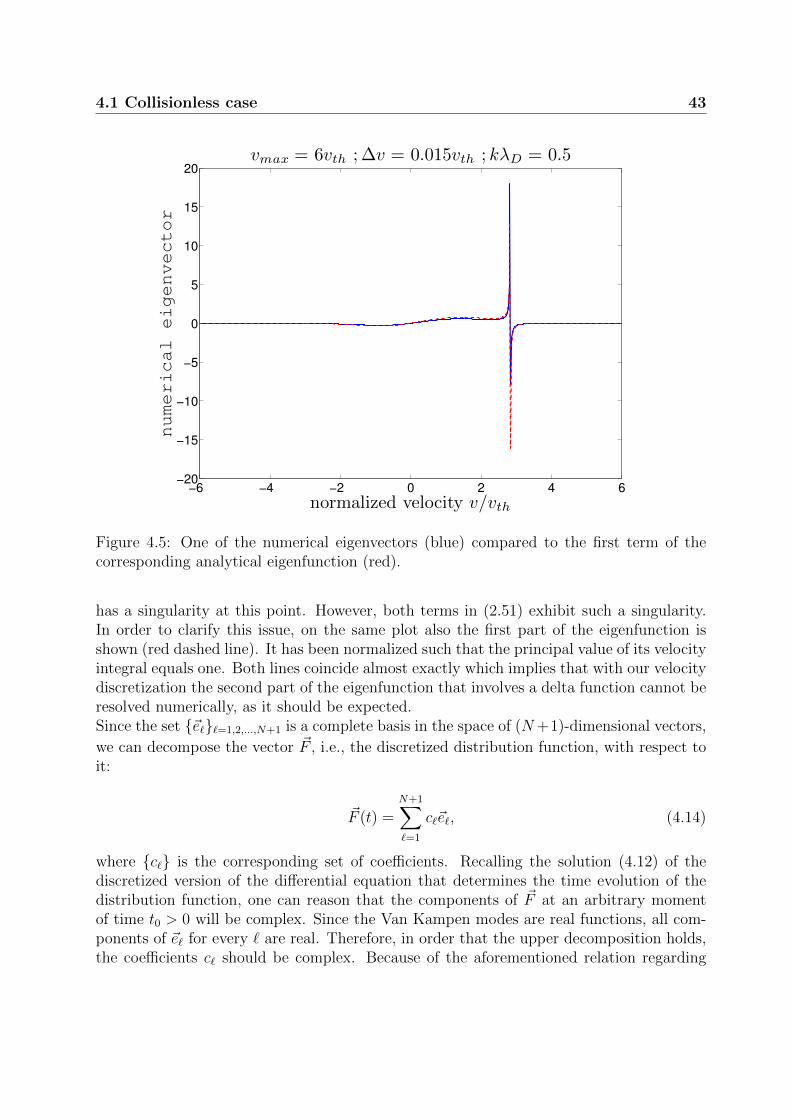
4.1 Collisionless case 43
−6 −4 −2 0 2 4 6−20
−15
−10
−5
0
5
10
15
20
normalized velocity v/vth
numerical eigenvector
vmax = 6vth ; ∆v = 0.015vth ; kλD = 0.5
Figure 4.5: One of the numerical eigenvectors (blue) compared to the first term of thecorresponding analytical eigenfunction (red).
has a singularity at this point. However, both terms in (2.51) exhibit such a singularity.In order to clarify this issue, on the same plot also the first part of the eigenfunction isshown (red dashed line). It has been normalized such that the principal value of its velocityintegral equals one. Both lines coincide almost exactly which implies that with our velocitydiscretization the second part of the eigenfunction that involves a delta function cannot beresolved numerically, as it should be expected.Since the set {~e`}`=1,2,...,N+1 is a complete basis in the space of (N+1)-dimensional vectors,
we can decompose the vector ~F , i.e., the discretized distribution function, with respect toit:
~F (t) =N+1∑
`=1
c`~e`, (4.14)
where {c`} is the corresponding set of coefficients. Recalling the solution (4.12) of thediscretized version of the differential equation that determines the time evolution of thedistribution function, one can reason that the components of ~F at an arbitrary momentof time t0 > 0 will be complex. Since the Van Kampen modes are real functions, all com-ponents of ~e` for every ` are real. Therefore, in order that the upper decomposition holds,the coefficients c` should be complex. Because of the aforementioned relation regarding

44 4. Numerical description of Langmuir waves
the scalar product between left and right eigenvectors and the new normalization we canwrite that
c`(t) =~g` · ~F (t)
~g` · ~e`. (4.15)
Here we have written the coefficients as functions of time, which they are. However, thereal and imaginary part of every coefficient change in such a way that, at least in the caseof Langmuir waves, |c`| is constant in time. Recalling (4.12), one can write
(~g` · ~e`)c`(t) = ~gT` ·(e−iMt · ~F0
)=(~gT` · e−iMt
)· ~F0 =
=
∞∑
n=1
(−it)nn!
~gT` ·Mn
︸ ︷︷ ︸=ωn` ~g
T`
· ~F0 = e−iω` t ~gT` · ~F0︸ ︷︷ ︸
∝c`(t=0)
= (~g` · ~e`)c`(t = 0)e−iω` t. (4.16)
Since, as we proved, in the case of Langmuir waves all eigenfrequencies are real, it isobvious that |c`(t)| = |c`(t = 0)| = const. One sees immediately that the absolute value
of the coefficients depends entirely on the initial value ~F0 of the discretized perturbationof the electron distribution function. In Figure 4.6 we have shown |c`| as a function of `
(i.e., ω`) for two different initial perturbations. The solid blue line corresponds tof1(k =
0.5, v, t = 0) = e−v2/2 and the black dashed line stands for an initial condition of the
formf1(k = 0.5, v, t = 0) = e−(v−1)2/2. The projections of the least damped Landau
solutions onto the real axis are indicated by the red dashed lines that help to comparetheir position with the position of the peaks. For the initial condition that is symmetricwith respect to v = 0 one sees that the largest coefficients lie around the projections of theleast damped Landau solutions. This hints at the importance of these Van Kampen modes.Qualitatively, the same behaviour is observed also in the case of an initial condition in theform of a Gauss curve centred at v = 1 (corresponding here to ω = 0.5). However, thistime the structure is not symmetric with respect to zero, as has to be expected.From this plot it is evident that the Van Kampen modes that lie directly above the leastdamped Landau roots are of vital importance for a successful description of the Langmuirwaves. This is the same conjecture that we arrived at after the investigation of the densityof eigenvalues shown in Figure 4.2. However, it is evident that also the Van Kampenmodes around zero have non-vanishing coefficients and should not be neglected. One cancheck the relative importance of the Van Kampen modes by removing parts of the initialcondition and then testing if the correct damping rate of the electric field is reproduced.One way to do this is to decompose the initial condition into Van Kampen modes and thento construct a new initial condition as as a sum of only some part of the Van Kampenmodes (including coefficients). For instance, we choose a centred Gauss curve as an initialcondition and divide the ω-axis in Figure 4.6 in five parts. The first part is from −3 to−2 and at first sight it should not be important since the the coefficients corresponding to

4.1 Collisionless case 45
−4 −3 −2 −1 0 1 2 3 40
0.01
0.02
0.03
0.04
0.05
0.06
0.07
0.08
0.09
0.1
ωℓ/ωpe
|cℓ|vmax = 6vth ; ∆v = 0.06vth ; kλD = 0.5
Figure 4.6: Coefficients corresponding to the decomposition of the perturbation of theelectron distribution function into (discrete) Van Kampen modes.
these modes are negligible. The next two parts are the areas ω ∈ (−2,−1) and ω ∈ (1, 2)which enclose the peaks and lie above the least damped Landau solutions. Last, there isthe middle part for ω ∈ (−1, 1) where the coefficients are considerably smaller than thoseat the two peaks but still not negligible. The last part is equivalent to the first one but forpositive ω. Let ~F0 be the full initial condition. Then we decompose it into Van Kampenmodes. The modified initial condition ~F0,new, e.g., for the middle part of the ω-axis is builtas
~F0,new =∑
ω∈(−1,1)
c`~e`. (4.17)
In the above expression, the sum is performed along those indices that correspond to thenormalized frequencies in (−1, 1). Figure 4.7 represents different modified initial condi-tions. From the form of the coefficients one could expect that an initial condition consistingof the Van Kampen modes with big coefficients should successfully reproduce the Landaudamping at least qualitatively. However, in Figure 4.7 a it is clear that in this case there isno exponential damping which means that the modes which we eliminated are important.The plot in Figure 4.7 b makes clear that even the Van Kampen modes around the twoleast damped Landau solutions put together cannot reproduce the Landau damping. For
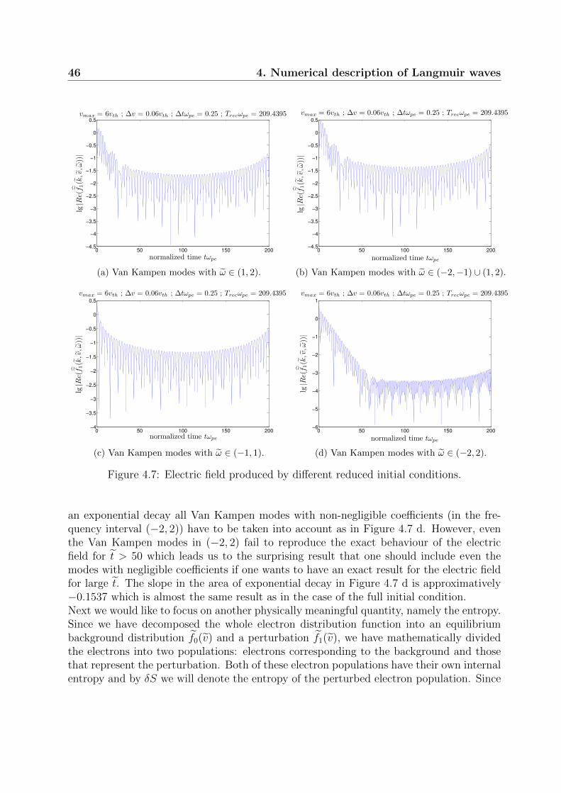
46 4. Numerical description of Langmuir waves
0 50 100 150 200−4.5
−4
−3.5
−3
−2.5
−2
−1.5
−1
−0.5
0
0.5
normalized time tωpe
lg|R
e( f 1(k,v,ω
))|
vmax = 6vth ; ∆v = 0.06vth ; ∆tωpe = 0.25 ; Trecωpe = 209.4395
(a) Van Kampen modes with ω ∈ (1, 2).
0 50 100 150 200−4.5
−4
−3.5
−3
−2.5
−2
−1.5
−1
−0.5
0
0.5
normalized time tωpe
lg|R
e( f 1(k,v,ω
))|
vmax = 6vth ; ∆v = 0.06vth ; ∆tωpe = 0.25 ; Trecωpe = 209.4395
(b) Van Kampen modes with ω ∈ (−2,−1) ∪ (1, 2).
0 50 100 150 200−4
−3.5
−3
−2.5
−2
−1.5
−1
−0.5
0
0.5
normalized time tωpe
lg|R
e( f 1(k,v,ω
))|
vmax = 6vth ; ∆v = 0.06vth ; ∆tωpe = 0.25 ; Trecωpe = 209.4395
(c) Van Kampen modes with ω ∈ (−1, 1).
0 50 100 150 200−6
−5
−4
−3
−2
−1
0
1
normalized time tωpe
lg|R
e( f 1(k,v,ω
))|
vmax = 6vth ; ∆v = 0.06vth ; ∆tωpe = 0.25 ; Trecωpe = 209.4395
(d) Van Kampen modes with ω ∈ (−2, 2).
Figure 4.7: Electric field produced by different reduced initial conditions.
an exponential decay all Van Kampen modes with non-negligible coefficients (in the fre-quency interval (−2, 2)) have to be taken into account as in Figure 4.7 d. However, eventhe Van Kampen modes in (−2, 2) fail to reproduce the exact behaviour of the electricfield for t > 50 which leads us to the surprising result that one should include even themodes with negligible coefficients if one wants to have an exact result for the electric fieldfor large t. The slope in the area of exponential decay in Figure 4.7 d is approximatively−0.1537 which is almost the same result as in the case of the full initial condition.Next we would like to focus on another physically meaningful quantity, namely the entropy.Since we have decomposed the whole electron distribution function into an equilibriumbackground distribution f0(v) and a perturbation f1(v), we have mathematically dividedthe electrons into two populations: electrons corresponding to the background and thosethat represent the perturbation. Both of these electron populations have their own internalentropy and by δS we will denote the entropy of the perturbed electron population. Since

4.1 Collisionless case 47
we have agreed to use a Maxwell distribution as f0(v), then for a fixed k δS reads [19]
δS =1
2
+∞∫
−∞
| f1(k, v, t)|2f0(v)
dv. (4.18)
If one denotes the vector corresponding to the discretized Maxwell distribution by ~F (M),then the last equation translates into
δS =∆v
2
N+1∑
n=1
|Fn|2
F(M)n
=∆v
2
N+1∑
n=1
∣∣∣∣∣N+1∑
`=1
c`e`,n
∣∣∣∣∣
2
1
F(M)n
=
=N+1∑
`=1
∆v
2|c`|2
N+1∑
n=1
|e`,n|2
F(M)n︸ ︷︷ ︸
=:δS`
+R =N+1∑
`=1
δS` +R, (4.19)
where e`,n is the nth component of ~e`. In this expression we have defined by δS` thequantity that represents the entropy corresponding to the jth Van Kampen mode and Rstands for the contribution of the cross-terms that arise when |∑ c`e`,n|2 is expanded. Ifone wants to approximate the whole entropy of the disturbed electron population via thesum of all δSj, then this leads to an error that equals R, which is the reason why we wouldlike to call R an error term. If one plots δS` with respect to the normalized frequency ω,one sees that the picture is qualitatively the same as in Figure 4.6. There are two largepeaks above the least damped Landau solutions and the other Van Kampen modes havemuch smaller entropy. However, one should note that the error term R is of considerableamplitude. This is a consequence of the non-orthogonality of the Van Kampen modes withrespect to the usual L2 scalar product. This issue of orthogonality is what we focus onnext. In [8] the claim is stated that with respect to the prescription
〈f(v), g(v)〉f0 :=
+∞∫
−∞
f(v)g(v)
f0
dv (4.20)
the Van Kampen modes corresponding to different frequencies are orthogonal to eachother. It is straightforward to prove explicitly that the prescription introduced in (4.20)defines a proper scalar product when f0(v) is positive definite, as in the case of a Maxwelldistribution.
We are going to test this conjecture and also compute the scalar product of the eigenmodeswith the usual L2 scalar product. For a Maxwellian background distribution the VanKampen eigenmodes are given by (2.51). Then we have for the two scalar products:
case 1) normal L2 scalar product, ω1 6= ω2:

48 4. Numerical description of Langmuir waves
⟨f 1,V (k, v, ω1),
f 1,V (k, v, ω2)
⟩
L2
:=
+∞∫
−∞
f 1,V (k, v, ω1)
f 1,V (k, v, ω2)dv =
=1
2πk2p.v.
+∞∫
−∞
v2e−v2
(kv − ω1)(kv − ω2)dv +
C2√2πk
p.v.
+∞∫
−∞
(−v)e−v2/2
kv − ω1
δ(kv − ω2)dv+
+C1√2πk
p.v.
+∞∫
−∞
(−v)e−v2/2
kv − ω2
δ(kv − ω1)dv + C1C2
+∞∫
−∞
δ(kv − ω1)δ(kv − ω2)dv
︸ ︷︷ ︸∝δ(ω1−ω2)=0 , since ω1 6=ω2
=
=1
2πk4p.v.
+∞∫
−∞
v2e−v2
(v − ω1
k)(v − ω2
k)dv+
1√2πk2(ω1 − ω2)
(C2ω2e
ω22/(2k
2) − C1ω1eω21/(2k
2))6= 0,
where Ci is defined as the velocity independent expression that multiplies the delta func-
tion in the second term off i,V as given in (2.51).
case 2) entropy scalar product, ω1 6= ω2:
⟨f 1,V (k, v, ω1),
f 1,V (k, v, ω2)
⟩
f0
:=
+∞∫
−∞
f 1,V (k, v, ω1)
f 1,V (k, v, ω2)
f0(v)dv =
=1
2πk2p.v.
+∞∫
−∞
v2e−v2/2
(kv − ω1)(kv − ω2)dv +
C2√2πk
p.v.
+∞∫
−∞
(−v)
kv − ω1
δ(kv − ω2)dv+
+C1√2πk
p.v.
+∞∫
−∞
(−v)
kv − ω2
δ(kv − ω1)dv + C1C2
+∞∫
−∞
δ(kv − ω1)δ(kv − ω2)
e−v2/2dv
︸ ︷︷ ︸∝δ(ω1−ω2)=0 , since ω1 6=ω2
=
=1√
2πk4p.v.
+∞∫
−∞
v2e−v2
(v − ω1
k)(v − ω2
k)dv +
1
k2(ω1 − ω2)(C2ω2 − C1ω1) = − 1
k26= 0.
Although this straightforward computation is not the most elegant way to make this pointclear, it is sufficient to show that the statement in [8] regarding the orthogonality of theeigenfunctions that correspond to different frequencies is apparently wrong. This meansthat the operator A, that we studied in chapter 3, is not symmetric also with respect tothe modified entropy scalar product. We can confirm our computation numerically. If nor-malized correctly, the ‘entropy’ scalar product of any two different numerical eigenvectors

4.1 Collisionless case 49
should give nearly 4 for k = 0.5 which the program eigenvalue.m yields. For differentvalues of the wave number the numerical results are also in agreement with the analyticalcomputation.At this point, it is useful to make a comment regarding the matrix M defined in (4.9).As it is known from Linear Algebra, one can find a scalar product under which the eigen-vectors of the matrix M corresponding to different eigenvalues are orthogonal if and onlyif M is normal, i.e., if M ·M∗ −M∗ ·M = 0, where the star denotes transposition andcomplex conjugation. In the collisionless case, the matrix has only real elements, so onesimply needs to transpose it. If one computes P = M ·M∗ −M∗ ·M and searches for theelement of P with the greatest absolute value, i.e., takes the supremum norm ‖P‖∞ of P ,then one sees that the elements of P get smaller when the resolution in velocity space getsbetter. It is easy to see numerically, as well analytically, that ‖P‖∞ scales linearly with∆v. At first sight, one would conclude that the matrix M gets closer to normality whenthe velocity resolution increases, and in the continuous limit, it should become normal,from which it follows that its eigenvectors are going to be orthogonal in this limit withrespect to some scalar product. However, in our numerical examination of the ‘entropy’scalar product between different eigenmodes there was no such scaling dependence on ∆v.In order to solve this puzzle, one should take into account the fact that the size of thematrix depends linearly on N . Thus, when velocity resolution is halved, the biggest ele-ment in P will also halve but, on the other hand, M , and therefore also P , will have fourtimes more elements. To take into account this fact, one should consider another normof P which include all matrix elements. An example of such a prescription is the ‘tracenorm’, ‖P‖2
tr := tr(P ∗ · P ). Practically, this is the sum of the absolute value squared ofall elements of P . The numerical computation for the case of Langmuir waves gives that‖P‖tr, having nearly the value of 14 for k = 0.5, stays constant and does not scale with ∆vin any way. Thus, even in the continuous limit the matrix M is not going to be normal.In this example one sees that if the limit process requires changing the size of the matrix,i.e., changing the operator, then the limit is by far not straightforward. We are going toencounter a similar problem later on in this work when dealing with the Lenard-Bernsteincollision operator in subsection 4.2.2.
4.1.2 ‘Bump-on-tail’ instability
Now, after we have tested our numerical scheme for reproducing known qualitative andquantitative results and gained confidence in its applicability to real problems in plasmaphysics, we will use this method to study the so called ‘bump-on-tail’ instability. In thecase of Langmuir waves in homogeneous collisionless plasma in global thermal equilibriumwe used as a background electron distribution a Maxwell distribution in velocity. Here, thisassumption is going to be modified by adding a second Maxwellian to it that correspondsto a different temperature and average velocity. Physically, this means that we have twodifferent electron populations in our plasma and they have different temperatures. Frombasic thermodynamics we know, of course, that in such cases both electron populations aregoing to interact with each other in such a way that a global thermal equilibrium is achieved,
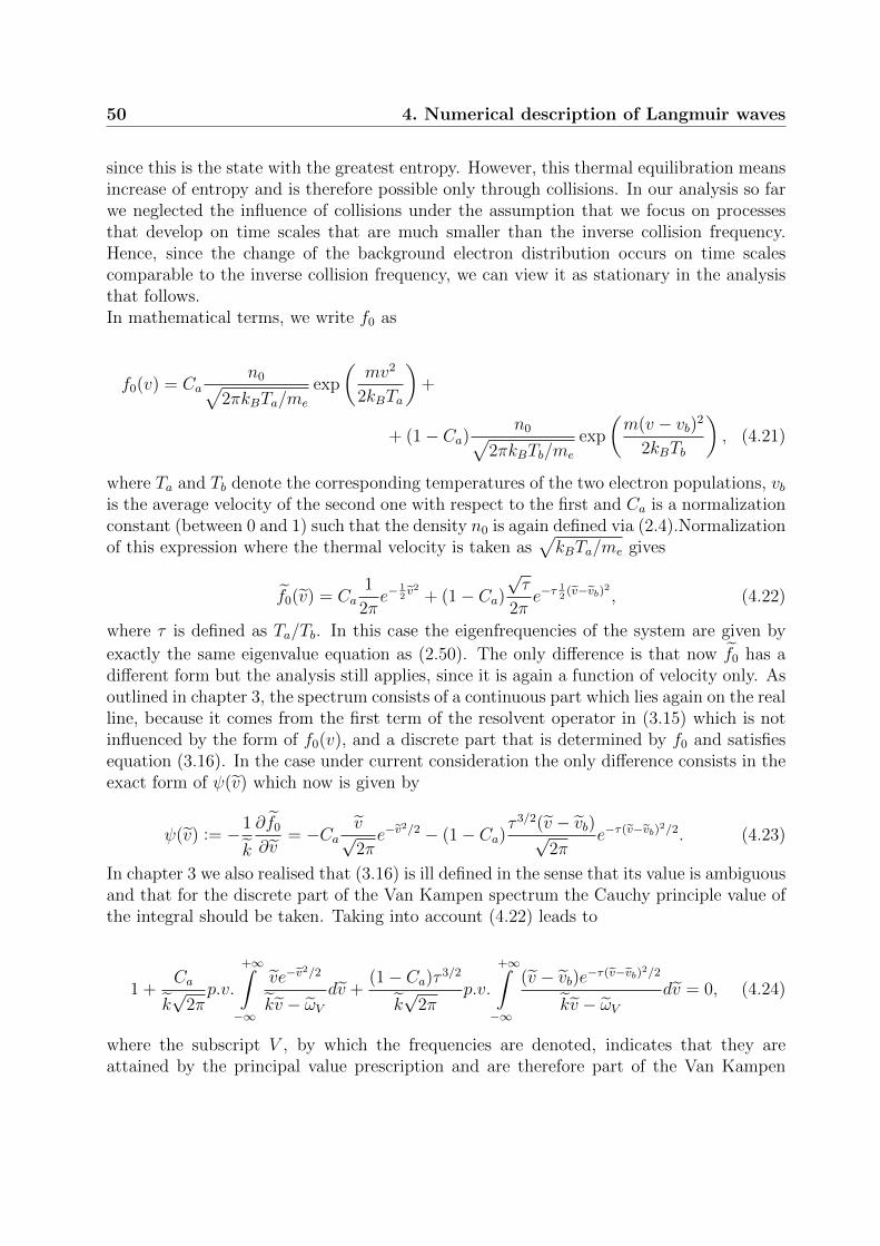
50 4. Numerical description of Langmuir waves
since this is the state with the greatest entropy. However, this thermal equilibration meansincrease of entropy and is therefore possible only through collisions. In our analysis so farwe neglected the influence of collisions under the assumption that we focus on processesthat develop on time scales that are much smaller than the inverse collision frequency.Hence, since the change of the background electron distribution occurs on time scalescomparable to the inverse collision frequency, we can view it as stationary in the analysisthat follows.In mathematical terms, we write f0 as
f0(v) = Can0√
2πkBTa/me
exp
(mv2
2kBTa
)+
+ (1− Ca)n0√
2πkBTb/me
exp
(m(v − vb)2
2kBTb
), (4.21)
where Ta and Tb denote the corresponding temperatures of the two electron populations, vbis the average velocity of the second one with respect to the first and Ca is a normalizationconstant (between 0 and 1) such that the density n0 is again defined via (2.4).Normalizationof this expression where the thermal velocity is taken as
√kBTa/me gives
f0(v) = Ca1
2πe−
12v2 + (1− Ca)
√τ
2πe−τ
12
(v−vb)2 , (4.22)
where τ is defined as Ta/Tb. In this case the eigenfrequencies of the system are given by
exactly the same eigenvalue equation as (2.50). The only difference is that now f0 has adifferent form but the analysis still applies, since it is again a function of velocity only. Asoutlined in chapter 3, the spectrum consists of a continuous part which lies again on the realline, because it comes from the first term of the resolvent operator in (3.15) which is notinfluenced by the form of f0(v), and a discrete part that is determined by f0 and satisfiesequation (3.16). In the case under current consideration the only difference consists in theexact form of ψ(v) which now is given by
ψ(v) := −1
k
∂f0
∂v= −Ca
v√2πe−v
2/2 − (1− Ca)τ 3/2(v − vb)√
2πe−τ(v−vb)2/2. (4.23)
In chapter 3 we also realised that (3.16) is ill defined in the sense that its value is ambiguousand that for the discrete part of the Van Kampen spectrum the Cauchy principle value ofthe integral should be taken. Taking into account (4.22) leads to
1 +Ca
k√
2πp.v.
+∞∫
−∞
ve−v2/2
kv − ωVdv +
(1− Ca)τ 3/2
k√
2πp.v.
+∞∫
−∞
(v − vb)e−τ(v−vb)2/2
kv − ωVdv = 0, (4.24)
where the subscript V , by which the frequencies are denoted, indicates that they areattained by the principal value prescription and are therefore part of the Van Kampen
4.1 Collisionless case 51
spectrum. On the other hand, in chapter 3 we derived that interpreting the integral in(3.16) as done along the Landau contour (‘Landau prescription’) gives the Landau solutions,denoted by ωL, that correspond to the t→ +∞ limit of the initial value problem, so nowwe simply write
1 +Ca
k√
2π
∫
L
ve−v2/2
kv − ωLdv +
(1− Ca)τ 3/2
k√
2π
∫
L
(v − vb)e−τ(v−vb)2/2
kv − ωLdv = 0 (4.25)
without undertaking the cumbersome analysis done previously in section 2.2. We willfocus our attention first on the last expression and transform it into a form that is moreconvenient to work with. Recalling the relations derived in the Appendix between the typeof integrals in the last equation and the plasma dispersion function, we note that
∫
L
ve−v2/2
kv − ωLdv =
√2π
k+
√2π
k
ωL
k√
2Z
(ωL
k√
2
); (4.26)
∫
L
(v − vb)e−τ(v−vb)2/2
kv − ωLdv =
√2π
k√τ
+
√2π
k
(ωL
k√
2− vb√
2
)Z
(√τ
2
(ωL
k√
2− vb√
2
)), (4.27)
which eventually leads to the following dispersion relation:
k2 + τ + Ca(1− τ) + CaωL
k√
2Z
(ωL
k√
2
)+
+ (1− Ca)τ√τ
2
(ωL
k− vb
)Z
(√τ
2
(ωL
k− vb
))= 0. (4.28)
Equation (4.28) is analogous to (2.38), which appeared in the study of Langmuir waves,and, as we shall see, the similarity in not only in the appearance but they also producesimilar sets of (countably infinitely many) solutions. The difference is that, because ofthe term involving vb, the set of solutions of (4.28) is not symmetric with respect to theimaginary axis and that for some values of the parameters Ca, τ , and vb, (4.28) can haveone unstable solution, while, as we already know, all solutions of (2.38) lie in the lower halfof the complex ω-plane. One easy way to find the solutions of (4.28) would be to proceedas in section 2.2 and to draw a contour plot of the absolute value of the function on theleft-hand side, which we will do later in this subsection.Before this we elaborate a little more on (4.24). The principal value integral can be viewedas a complex valued function of the complex argument ωV and we will split it into real andimaginary part in order to gain some insights into this mathematical expression. Since thetwo integrals are of the same type, we treat only the first one:
52 4. Numerical description of Langmuir waves
g(ωV ) := p.v.
+∞∫
−∞
ve−v2/2
v − ωV /kdv = p.v.
+∞∫
−∞
v(v − ω∗V /k)e−v2/2
|v − ωV /k|2dv =
= p.v.
+∞∫
−∞
v(v − ωV r/k)e−v2/2
|v − ωV /k|2dv + i
ωV i
kp.v.
+∞∫
−∞
ve−v2/2
|v − ωV /k|2dv, (4.29)
where the asterisk denotes complex conjugation and ωV r,i denote the real and imaginarypart of ω, respectively. From the above computation it follows immediately that g∗(ωV ) =g(ω∗V ). At this point we may tend to think that the above conclusion was obvious. However,it is noteworthy that at first sight such a simple relation seems obvious also when we do theintegral in question along the Landau contour but such a conclusion would be wrong. Inthe case of the Landau prescription the integral is related to the plasma dispersion functionvia (4.26) and Z does not have this simple property when complex conjugated but insteadZ(ξ∗) = −Z∗(−ξ) [1]. A completely analogous computation leads to the same result forthe second integral, which we will denote by gτ (ωV ), namely that g∗τ (ωV ) = gτ (ω
∗V ). In
terms of this notation (4.24) can be rewritten as
k√
2π + Cag(ωV ) + (1− Ca)τ 3/2gτ (ωV ) = 0. (4.30)
Taking the complex conjugate of both sides and using the relations we just derived, wearrive at
k√
2π + Cag(ω∗V ) + (1− Ca)τ 3/2gτ (ω∗V ) = 0, (4.31)
which means that, if ωV is a solution of (4.24), then so is ω∗V . In other words, the discretepart of the Van Kampen spectrum possesses a mirror symmetry with respect to the realaxis. Since the whole spectrum consists of the union of the continuous part situated onthe real line and the discrete part given by (4.24), then this mirror symmetry applies tothe whole Van Kampen spectrum but is absent for the set of Landau solutions ωL.Last, we derive analytically another interesting property of the solutions of (4.24) and(4.28). For this we go back to the definition of the Landau contour. It is constructed insuch a way that the integration path goes from −∞ to +∞ and encircles the poles of theintegrand in the anticlockwise direction if they lie on the real line or in the lower half planeas shown in Figure 2.1. In the problem under consideration, the integrands in (4.24) and
(4.28) have only one pole, namely v =ωV,L
k. If there are solutions of the equations with
positive imaginary part (that in our convention corresponds to instability), then both theCauchy principal value and the Landau contour reduce to a normal integration along thereal line, since in that case the position of the pole resolves all ambiguities. From this, itfollows immediately that the unstable solutions of (4.24) and (4.28) are the same.For a numerical evaluation of (4.28) we use the same idea as outlined in section 2.2 (im-plemented in MATLAB with the program bump landau.m shown in the Appendix) which

4.1 Collisionless case 53
gives us a contour plot of the absolute value of the left-hand side of the equation. Herethe corresponding function was also evaluated on a quadratic grid with the resolution of∆ω = 0.001 and 5 contours have been drawn on equidistant heights from 0 to 0.02.For numerical reproduction of the Van Kampen spectrum we again discretize the velocityaxis as described extensively in subsection 4.1.1. The only difference here lies in the formof G, namely
G(v) = − Cav√2πe−v
2/2 − (1− Ca)τ 3/2(v − vb)√2π
e−τ(v−vb)2/2. (4.32)
The corresponding spectrum is shown in Figure 4.8 (produced with the programs bump.mand landau bump.m that can be found in the Appendix) together with a contour plot of
the Landau solutions and the numerical parameters (k, vmax, ∆v, Ca, vb and τ) needed toreproduce them. The Van Kampen eigenvalues are indicated by blue crosses.
−3 −2 −1 0 1 2 3−1
−0.8
−0.6
−0.4
−0.2
0
0.2
0.4
Re(ω)/ωpe
Im(ω
)/ωpe
vmax = 6vth ; ∆v = 0.06vth ;Ca = 0.7 ; vb = 4vth ; τ = 2
Figure 4.8: Landau solutions and Van Kampen spectrum for the case of ‘bump-on-tail’instability (k = 0.5).
One sees immediately that our numerical scheme preserves the symmetry of the spectrum,which we derived analytically. This fact can be understood easily. For this one should recallthe form of the matrix M defined in (4.9). The first two terms represent the multiplicationoperator A0 analysed in chapter 3 and all the parameters in front of the matrices I andB are, of course, real. By the transition from Langmuir waves to the ‘bump-on-tail’

54 4. Numerical description of Langmuir waves
distribution only the last term has changed its particular form but, as a derivative of thereal function f0(v), it is still real. Therefore, all elements in M are real numbers. Theeigenvalues of M , the set of which is intended to serve as an approximation of the VanKampen spectrum, are determined as solutions of the polynomial equation
det(M − ωV I) = 0. (4.33)
Since all elements of M are real, it follows that also all coefficients in the polynomialdet(M − ωI) (formed via multiplications and additions/subtractions of elements of M) arereal. In this case it is clear that, if ωV is a solution of (4.33), then so is ω∗V . In other words,our numerical scheme, based on discretization of the velocity axis, preserves the symmetryof the continuous equations, that we are trying to approximate. Since this is not alwaysthe case in numerics, this observation help us gain even more confidence in our approach.Another feature of our numerical evaluation, that is clearly seen in Figure 4.8, is that theposition of the unstable Van Kampen eigenvalues seem to coincide with the position of theunstable Landau solutions as we already predicted analytically. This result can be verifiedmore precisely. Since we have already computed the exact position of the unstable VanKampen eigenvalue, we only need the exact position of the unstable Landau solution onthe complex plane. From the contour plot we can derive the value of ωL with practicallyarbitrary precision (up to the computer limit, of course). For the unstable solution onefinds numerically
ωV ≈ 1.194 + 0.105i ; ωL ≈ 1.194 + 0.104i. (4.34)
These frequencies have been computed with almost the same parameters as those used toproduce Figure 4.8. The only change, that has been made, was that for the sake of betterprecision the number of points on the velocity axis was set to 2000. This comparisondemonstrates that our numerical analysis reproduces the analytical results quite well. Theminor difference in the imaginary parts of the two solutions, which is on the order of10−3, is most probably due to the numerical resolution in velocity space which is good butnevertheless finite.After this quick mathematical analysis of the ‘bump-on-tail’ instability, it is worth toelaborate on its physical meaning. In section 2.1 we discussed a simplified model of theinteraction between an electrostatic wave and a plasma. We discovered that the collisionlessdamping is a resonant effect and that it depends on the slope of f0(v) at the point thatcorresponds to the wave frequency. For a centred Gauss curve it was not possible to have anenergy transfer from the particles to the wave because the derivative of the Gauss functionhas always the opposite sign of the argument for which it is taken and, therefore, theproduct v0 ∂f0/∂v|v=v0
is always negative. However, in the case of two combined Maxwelldistributions, like here, there can be some set of parameters for which this product ispositive. Such a situation is shown in Figure 4.9. In the interval between the two reddashed lines the derivative of the function and its argument at the corresponding point havethe same signs which is a necessary condition for an instability. If there is an electrostaticwave in the plasma with frequency and wave number such that ω/k lie in the interval

4.2 Introducing collision operators 55
−6 −4 −2 0 2 4 60
0.05
0.1
0.15
0.2
0.25
0.3
0.35
normalized velocity v/vth
f 0(v)
Ca = 0.7 ; vb = 4vth ; τ = 2
Figure 4.9: Background distribution function f0(v) in the case of ‘bump-on-tail’ instability.
limited by the red lines, then the wave decelerates more particles than is accelerates and,thus, gains energy which is equivalent to an instability. For these parameters the frequencyof the instability in Figure 4.8 corresponds to a phase velocity that is at the beginning ofthis interval.
4.2 Introducing collision operators
In this section we go one step further toward a better physical model by introducingcollisions into our system. Since we are working with a one dimensional system, there arenot many choices available. The reason for this is that only few collision operators can beformulated in one dimension.
4.2.1 Krook model
The first collision operator which we introduce is the so called Bhatnagar-Gross-Krookcollision operator introduced in [17] which in mathematical terms is given by
(∂f
∂t
)
col
= −ν(f(z, v, t)− f0(v)), (4.35)

56 4. Numerical description of Langmuir waves
where ν is the collision frequency. This is a very simple and minimalistic model for colli-sions. One can easily see (by computing the 0th, 1st and 2nd velocity moment of (4.35))that this collision operator satisfies neither particle, nor momentum, nor energy conserva-tion which are fundamental physical constraints. However, because of its simple form, itis widely used in plasma physics and especially in fluid theory and often allows physicalinsights into the role of collisions. Therefore, we are going to use it and see how it altersour system.Recalling (2.3), it is immediately clear that this collision operator is proportional tof1(z, v, t). A natural normalization for ν would be the plasma frequency ωpe. With this,the normalized and linearised Boltzmann equation reads
∂f1
∂t+ v
∂f1
∂z− E(z, t)
∂f0
∂v= −νf1(z, v, t), (4.36)
where the electric field is again determined by (2.13). In order to solve this equationtogether with (2.13) we make a Fourier transform of both equations in space and in timeby using the same conventions as in (2.14) and (2.49). This leads to
(ω − iν)f1(k, v, ω) = kv
f1(k, v, ω)− 1
k
∂f0
∂v
+∞∫
−∞
f1(k, v, ω)dv. (4.37)
This is an eigenvalue equation from the same type as (2.50). The only difference is that thenormalized frequency on the right is modified by the term iν. Nevertheless, the mathemat-ical problem consists in finding the eigenvalues of the linear operator on the right-hand sideof (4.37) and this operator is the same as in (2.50), so we already know that its spectrumis the entire real line, i.e., ω∗ := ω + iν is real. This immediately leads to the conclusionthat the imaginary part of ω equals −iν. In other words, the effect of the Bhatnagar-Gross-Krook collision operator on our simple system was to shift the whole Van Kampenspectrum shown in Figure 4.1 downwards by ν. This means that now all Van Kampenmodes are individually damped by a damping rate of ν which adds to the Landau damp-ing. One can also easily compute the electric field in this model and produce a plot that isanalogous to the one in Figure 4.4. The only difference will be that the collision frequencywill accelerate the damping such that the new growth rate will be Im(ωL)− ν.
4.2.2 Lenard-Bernstein model
In this subsection, we consider another type of collision operator named after A. Lenardand I. B. Bernstein that can also be formulated in a one-dimensional velocity space. To thebest of our knowledge it has been applied to one-dimensional Langmuir waves for first timein [18]. However, this subsection was inspired primarily by [15] where the authors showthat in this model the Van Kampen spectrum is altered profoundly. In this subsection thisclaim is tested with a different numerical scheme and after confirming their result we makeand additional step and investigate which part of the collision operator is responsible for

4.2 Introducing collision operators 57
the qualitative changes observed.The linearised Lenard-Bernstein collision operator is given by
(∂f
∂t
)
col,1
= νf1(z, v, t) + νv∂f1(z, v, t)
∂v+ νv2
th
∂2f1(z, v, t)
∂v2, (4.38)
where ν is again the collision frequency which in this model is taken to be independent of theparticle velocity. The collision operator introduced in (4.38) has important advantages froma physical point of view compared to (4.35). It conserves the number of particles, satisfiesthe H theorem, and preserves the velocity space diffusion which also characterizes themore comprehensive Fokker-Planck collision operator. This model of introducing collisionaleffects in our system fulfils some fundamental physical constraints and is therefore muchmore realistic than the one considered in subsection 4.2.1. The normalization of (4.38)using the quantities defined in (2.11) is straightforward and one arrives at
∂f1
∂t+ v
∂f1
∂z− E(z, t)
∂f0
∂v= ν
(f1(z, v, t) + v
∂f1(z, v, t)
∂v+∂2f1(z, v, t)
∂v2
)(4.39a)
∂E(z, t)
∂z= −
+∞∫
−∞
f1(z, v, t)dv. (4.39b)
We approach this system of equations in the same way as we did in the previous cases:through a Fourier transformation in space and time according to (2.14) and (2.49). Thisallows us to substitute the transformed second equation into the first one, so we are leftwith
ωf1 = kv
f1 −
1
k
∂f0
∂v
+∞∫
−∞
f1(..., v, ...)dv + iν
f1 + v
∂f1
∂v+∂2 f1
∂v2
. (4.40)
This equation can also be viewed as an eigenvalue equation where the right-hand side of
(4.40) represents a linear operator acting onf1(k, v, ω). The first part of this operator is
the one defined in (3.1) as A which we already analysed thoroughly in 3. The second part,proportional to the collision frequency, can be viewed as a perturbation of A which we willdenote by iνP . With this notation (4.40) can be written as
ωf1(k, v, ω) = ((A+ iνP )
f1)(k, v, ω). (4.41)
In order to solve the problem via the Van Kampen approach we have to find the spectrum ofthe perturbed operator A+iνP . In principle, we can try to find the corresponding resolventoperator R(ω, A+ iνP ) and then search for its poles. When we have the poles, we can thenstudy how the spectrum changes in the limit ν → 0. However, because of the complicatedform of the operator which involves a multiplication, integral and differential operators,

58 4. Numerical description of Langmuir waves
such an approach is not straightforward in this case. Instead, we will approach the problemnumerically by again discretizing the velocity axis which will turn the continuous operatorinto a matrix and then find the eigenvalues, the set of which is the Van Kampen spectrum,of this matrix numerically. At first sight, it might look obvious that in the limit ν → 0one should recover the usual continuous Van Kampen spectrum consisting of the entirereal line. Nevertheless, this naive way of thinking would be correct only if the resolventR(ω, A+ iνP ) is a continuous function of ν (or at least continuous in some small intervalaround ν = 0). We cannot be certain of that, since we do not know how R(ω, A + iνP )looks like. Our numerical evaluation will show that indeed the limit ν → 0 is non-trivialwhich suggests a discontinuity of the resolvent operator at ν = 0. From a physical pointof view this means that collisions, no matter how small the collision frequency, alter thesystem profoundly (at least when modelled using the Lenard-Bernstein collision operator).Since we already derived a matrix approximation for A, we now have to consider only theperturbation P . The first part of it is just the identity operator, for which we use, of course,the identity matrix. For a discrete implementation of the first and second derivatives weuse a centred scheme given by
∂
f1
∂v
j
=Fj+1 − Fj−1
2∆v;
∂
2 f1
∂v2
j
=Fj+1 − 2Fj + Fj−1
∆v2, (4.42)
where the vector ~F is the discrete representation off1(k, v, ω) when v → vj and is defined
in subsection 4.1.1. The vector {Fj+1} can be produced from ~F by shifting its componentsone position upwards:
X+1 · ~F :=
0 1 0 · · · 00 0 1 · · · 0...
......
. . ....
0 0 0 · · · 10 0 0 · · · 0
F1
F2
F3...
FN+1
=
F2
F3...
FN+1
0
, (4.43)
where we have erased F1. It is noteworthy that the last component of the new vector is
set to zero. From a physical point of view, however, it is clear thatf1 does not fall to
zero for v > vmax but from our previous analysis we know thatf1 → 0 for |v| → +∞
since the integral∫ +∞−∞ |
f1|dv has to converge. For this to be true
f1 has to decrease rapidly
enough when v increases. In order to make our statements a little more precise we write thediscrete form of the previous integral but this time with 0 and +∞ as limits of integration,which does not influence the conclusions we are about to make:
+∞∫
0
| f1|dv → ∆v∞∑
j=1
|Fj| <∞. (4.44)

4.2 Introducing collision operators 59
For this to be true the condition limj→∞
|Fj+1||Fj | < 1 must hold which implies that, for j suffi-
ciently large, |Fj+1| < |Fj|. Recalling (4.42), it also follows that for large j
∣∣∣∣∣∣
∂
f1
∂v
j
∣∣∣∣∣∣=|Fj+1 − Fj−1|
2∆v≤ |Fj−1|
∆v, (4.45)
which means that our centred equidistant derivative should fall for large v at least as
rapidly asf1. This means that setting the last component in the vector on the right-hand
side of (4.43) to zero is a small mistake if N is sufficiently large. Thus, the discretizedderivatives in matrix notation can be written as
∂f1
∂v→ 1
2∆v(X+1 −X−1) · ~F ; (4.46)
∂2 f1
∂v2→ 1
∆v2(X+1 − 2I +X−1) · ~F , (4.47)
where I is the identity matrix of dimension N + 1 and X−1 is defined as
X−1 :=
0 0 · · · 0 01 0 · · · 0 00 1 · · · 0 0...
.... . .
......
0 0 · · · 1 0
. (4.48)
The first derivative in the expression for P is multiplied by v. In subsection 4.1.1 we sawthat in the discrete case this is achieved by a multiplication with the matrix −vmax (N+2)
NI+
∆vB with B defined as in the corresponding subsection. Therefore, the matrix approxi-mation of (4.41) can be written as
ω ~F =
[M + iν
(I +
1
2∆v
(−vmax
(N + 2)
NI + ∆vB
)· (X+1 −X−1)+
+1
∆v2(X+1 − 2I +X−1)
)]· ~F =: Mν · ~F , (4.49)
where M is defined in (4.9). This matrix eigenvalue equation can be implemented easilyusing MATLAB. Four results of such an implementation for ν = 0.01, achieved with theprogram Lenard Bernstein.m which can be found in the Appendix, are shown in Figure4.11. One sees that all Van Kampen modes (represented by blue crosses) lie in the lowerhalf of the complex ω-plane, i.e., they are damped. If we try to investigate the limit ν → 0by just computing this spectrum for smaller and smaller ν without changing the size ofthe matrix on the right-hand side of (4.49), then the result would be that all eigenvalues

60 4. Numerical description of Langmuir waves
of the collisional spectrum will tend to the real axis. This can be easily understood asfollows. The numerical Van Kampen eigenvalues are defined as the solutions of the equationdet(Mν − ωI) = 0. From the definition of Mν in (4.49) it is clear that all elements of thismatrix are analytic functions of ν which implies that also all coefficients of the polynomialdet(Mν−ωI) are analytic functions of the collision frequency. In this case one can be certain[6, p. 4, Theorem XII.2] that the position of the eigenvalues is a continuous function of ν.More precise, if for a given value ν0 there is an eigenvalue, say ω0, with multiplicity m,then for ν1 close to ν0 there are going to be eigenvalues in the immediate vicinity of ω0
and the sum of their multiplicity is m. However, such a limit, although reasonable from amathematical point of view, does not reproduce the right physics. We already know thatthe Van Kampen modes in the collision free case involve a delta function in velocity space.This means that for ν = 0 there exist arbitrary small structures in velocity space.
−6 −4 −2 0 2 4 60
0.5
1
1.5
normalized velocity v/vth
|f1(v)|
vmax = 6vth; ν = 0.01ωpe ;N = 500
Figure 4.10: Typical eigenvector corresponding to the discretized form of A+ iνP .
If collisions are present in our model, they make the eigenfunctions smooth with respectto the velocity [16]. When the collision frequency tends to zero, the structures in velocityspace get smaller. In order to make physically meaningful conclusions, we must be able toresolve these structures, i.e., we must increase the numerical resolution in velocity space(i.e., number of points in the interval [−vmax, vmax]) when we decrease ν. Therefore, oneshould always change the operator while performing the limit ν → 0. This has to be done insuch a way that the resolution is always sufficiently high. First we should give ‘sufficientlyhigh’ a more precise explanation. As already mentioned, for ν = 0 the eigenfunction of the
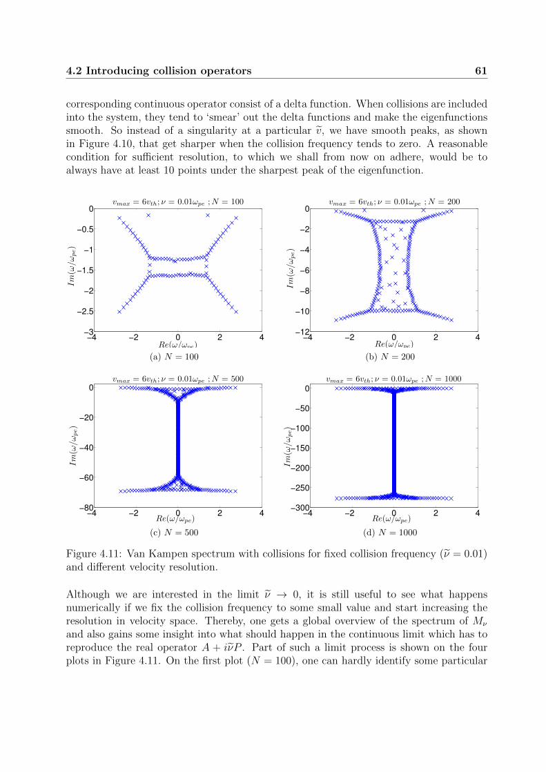
4.2 Introducing collision operators 61
corresponding continuous operator consist of a delta function. When collisions are includedinto the system, they tend to ‘smear’ out the delta functions and make the eigenfunctionssmooth. So instead of a singularity at a particular v, we have smooth peaks, as shownin Figure 4.10, that get sharper when the collision frequency tends to zero. A reasonablecondition for sufficient resolution, to which we shall from now on adhere, would be toalways have at least 10 points under the sharpest peak of the eigenfunction.
−4 −2 0 2 4−3
−2.5
−2
−1.5
−1
−0.5
0
Re(ω/ωpe)
Im(ω
/ωpe)
vmax = 6vth; ν = 0.01ωpe ;N = 100
(a) N = 100
−4 −2 0 2 4−12
−10
−8
−6
−4
−2
0
Re(ω/ωpe)
Im(ω
/ωpe)
vmax = 6vth; ν = 0.01ωpe ;N = 200
(b) N = 200
−4 −2 0 2 4−80
−60
−40
−20
0
Re(ω/ωpe)
Im(ω
/ωpe)
vmax = 6vth; ν = 0.01ωpe ;N = 500
(c) N = 500
−4 −2 0 2 4−300
−250
−200
−150
−100
−50
0
Re(ω/ωpe)
Im(ω
/ωpe)
vmax = 6vth; ν = 0.01ωpe ;N = 1000
(d) N = 1000
Figure 4.11: Van Kampen spectrum with collisions for fixed collision frequency (ν = 0.01)and different velocity resolution.
Although we are interested in the limit ν → 0, it is still useful to see what happensnumerically if we fix the collision frequency to some small value and start increasing theresolution in velocity space. Thereby, one gets a global overview of the spectrum of Mν
and also gains some insight into what should happen in the continuous limit which has toreproduce the real operator A + iνP . Part of such a limit process is shown on the fourplots in Figure 4.11. On the first plot (N = 100), one can hardly identify some particular

62 4. Numerical description of Langmuir waves
structure of the spectrum. However, as the resolution is increased, it becomes apparentthat the spectrum consists of three different parts. Some of the eigenvalues form two lineswhich are parallel to the real line. The first such line is just below the real axis and thesecond one is on the other side of the spectrum and its imaginary part increases nearlyquadratically with N . The rest of the eigenvalues form a line on the imaginary ω-axis thatconnects the other two groups of eigenvalues. From this global overview of the spectrum,we see also two other distinctive features. First, there are points that separate from the restof the spectrum and their position appears to be in the vicinity of the two least dampedLandau solutions that are shown in Figure 2.3. This foreshadows the correctness of thestatement that in the ν → 0 limit these Van Kampen eigenvalues will tend to the leastdamped Landau solutions.Looking at Figure 4.11, one also notices that for fixed resolution, there is always some areain the spectrum where the eigenvalues are distributed stochastically. From the theoreticalmodel it is known [16] that, if ωr + iωi is an eigenvalue, then so is −ωr + iωi. However,this symmetry is not observed in the central area of the first two plots which leads usto the conjecture that the distribution of eigenvalues there is not physical but is ratherdue to some numerical effect. Increasing the resolution, this area shrinks and divides intotwo parts when some of the eigenvalues align on the imaginary axis. When we investigatethe limit process of decreasing collision frequency later on, we will ensure that all Landausolutions lie outside this area of stochasticity in order to be certain that no Van Kampeneigenvalues approach a Landau solution randomly. This imposes a lower limit on the res-olution in velocity space that is stricter than the one we determined while discussing theform of the eigenfunctions.
Numerical limit ν → 0
Now, after we have made ourselves familiar with some general properties of the discretizedVan Kampen spectrum, we focus on the issue of the ν → 0 limit. In order to gain someinsight into what happens qualitatively, we have shown in Figure 4.12 the same part of thecomplex ω-plane for different collision frequencies. Here the resolution in velocity spacehas been chosen to satisfy the last convergence condition discussed above. It should benoted also that these plots are produced for k = 0.5. The blue crosses represent again theVan Kampen eigenvalues and the red circles denote the Landau solutions for collisionlessplasma. In order to achieve better resolution in velocity space while having the samematrix size, we have taken a smaller interval in velocity space, namely −4 < v < 4. Thiswill be useful when taking the limit ν → 0, since it allows us to go to smaller values of thecollision frequency with the same computational power.One sees clearly how two of the Van Kampen eigenvalues get closer and closer to the leastdamped Landau solutions when the collision frequency decreases. In order to validate thisassumption and to make it mathematically more precise, one can compute the absolutevalue of the difference ω between one of the least damped Landau solution (here theone with positive real part) and the corresponding Van Kampen eigenvalue for a set ofcollision frequencies. The results of such a computation (the blue stars) are shown in
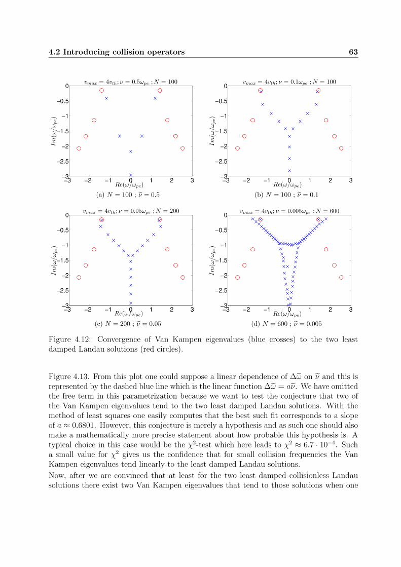
4.2 Introducing collision operators 63
−3 −2 −1 0 1 2 3−3
−2.5
−2
−1.5
−1
−0.5
0
Re(ω/ωpe)
Im(ω
/ωpe)
vmax = 4vth; ν = 0.5ωpe ;N = 100
(a) N = 100 ; ν = 0.5
−3 −2 −1 0 1 2 3−3
−2.5
−2
−1.5
−1
−0.5
0
Re(ω/ωpe)
Im(ω
/ωpe)
vmax = 4vth; ν = 0.1ωpe ;N = 100
(b) N = 100 ; ν = 0.1
−3 −2 −1 0 1 2 3−3
−2.5
−2
−1.5
−1
−0.5
0
Re(ω/ωpe)
Im(ω
/ωpe)
vmax = 4vth; ν = 0.05ωpe ;N = 200
(c) N = 200 ; ν = 0.05
−3 −2 −1 0 1 2 3−3
−2.5
−2
−1.5
−1
−0.5
0
Re(ω/ωpe)
Im(ω
/ωpe)
vmax = 4vth; ν = 0.005ωpe ;N = 600
(d) N = 600 ; ν = 0.005
Figure 4.12: Convergence of Van Kampen eigenvalues (blue crosses) to the two leastdamped Landau solutions (red circles).
Figure 4.13. From this plot one could suppose a linear dependence of ∆ω on ν and this isrepresented by the dashed blue line which is the linear function ∆ω = aν. We have omittedthe free term in this parametrization because we want to test the conjecture that two ofthe Van Kampen eigenvalues tend to the two least damped Landau solutions. With themethod of least squares one easily computes that the best such fit corresponds to a slopeof a ≈ 0.6801. However, this conjecture is merely a hypothesis and as such one should alsomake a mathematically more precise statement about how probable this hypothesis is. Atypical choice in this case would be the χ2-test which here leads to χ2 ≈ 6.7 · 10−4. Sucha small value for χ2 gives us the confidence that for small collision frequencies the VanKampen eigenvalues tend linearly to the least damped Landau solutions.
Now, after we are convinced that at least for the two least damped collisionless Landausolutions there exist two Van Kampen eigenvalues that tend to those solutions when one
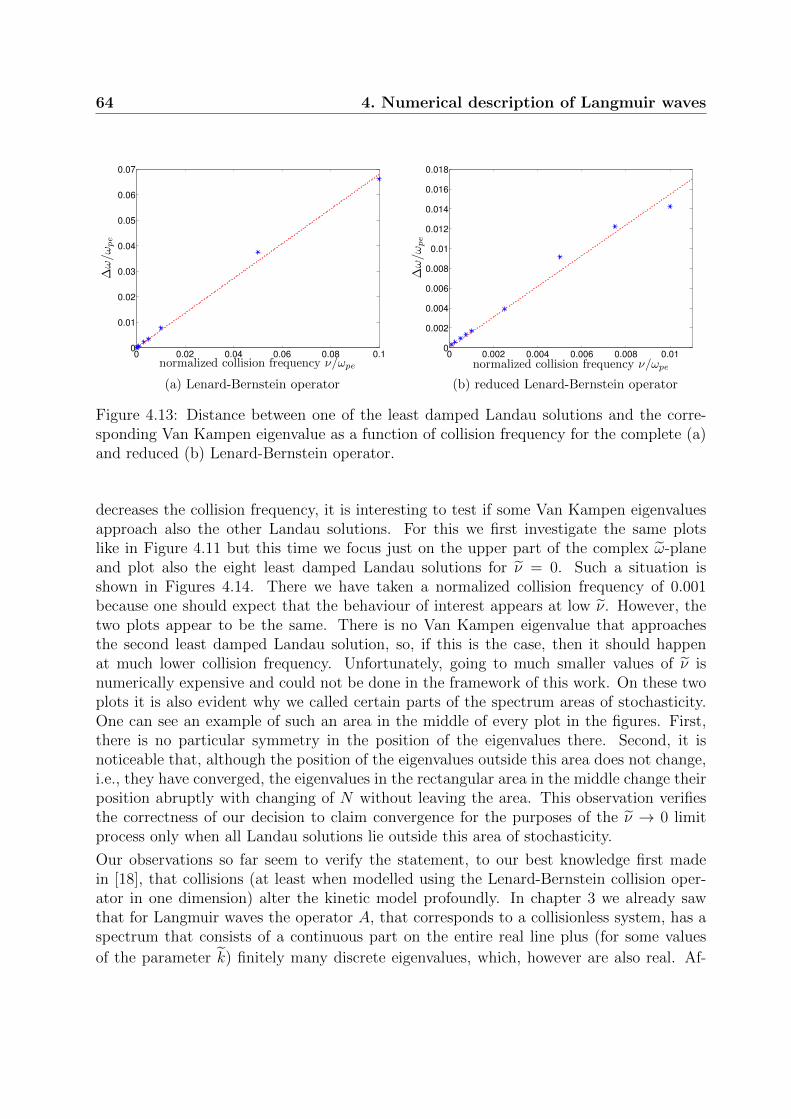
64 4. Numerical description of Langmuir waves
0 0.02 0.04 0.06 0.08 0.10
0.01
0.02
0.03
0.04
0.05
0.06
0.07
normalized collision frequency ν/ωpe
∆ω/ωpe
(a) Lenard-Bernstein operator
0 0.002 0.004 0.006 0.008 0.010
0.002
0.004
0.006
0.008
0.01
0.012
0.014
0.016
0.018
normalized collision frequency ν/ωpe
∆ω/ωpe
(b) reduced Lenard-Bernstein operator
Figure 4.13: Distance between one of the least damped Landau solutions and the corre-sponding Van Kampen eigenvalue as a function of collision frequency for the complete (a)and reduced (b) Lenard-Bernstein operator.
decreases the collision frequency, it is interesting to test if some Van Kampen eigenvaluesapproach also the other Landau solutions. For this we first investigate the same plotslike in Figure 4.11 but this time we focus just on the upper part of the complex ω-planeand plot also the eight least damped Landau solutions for ν = 0. Such a situation isshown in Figures 4.14. There we have taken a normalized collision frequency of 0.001because one should expect that the behaviour of interest appears at low ν. However, thetwo plots appear to be the same. There is no Van Kampen eigenvalue that approachesthe second least damped Landau solution, so, if this is the case, then it should happenat much lower collision frequency. Unfortunately, going to much smaller values of ν isnumerically expensive and could not be done in the framework of this work. On these twoplots it is also evident why we called certain parts of the spectrum areas of stochasticity.One can see an example of such an area in the middle of every plot in the figures. First,there is no particular symmetry in the position of the eigenvalues there. Second, it isnoticeable that, although the position of the eigenvalues outside this area does not change,i.e., they have converged, the eigenvalues in the rectangular area in the middle change theirposition abruptly with changing of N without leaving the area. This observation verifiesthe correctness of our decision to claim convergence for the purposes of the ν → 0 limitprocess only when all Landau solutions lie outside this area of stochasticity.
Our observations so far seem to verify the statement, to our best knowledge first madein [18], that collisions (at least when modelled using the Lenard-Bernstein collision oper-ator in one dimension) alter the kinetic model profoundly. In chapter 3 we already sawthat for Langmuir waves the operator A, that corresponds to a collisionless system, has aspectrum that consists of a continuous part on the entire real line plus (for some values
of the parameter k) finitely many discrete eigenvalues, which, however are also real. Af-
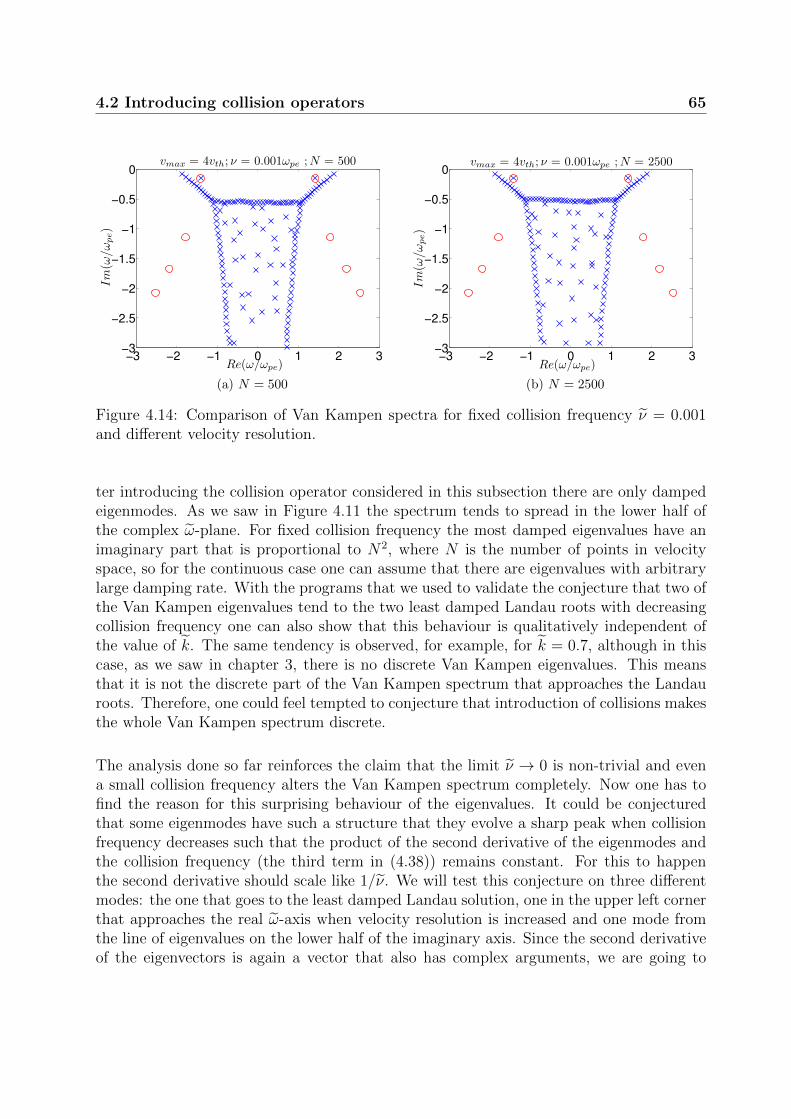
4.2 Introducing collision operators 65
−3 −2 −1 0 1 2 3−3
−2.5
−2
−1.5
−1
−0.5
0
Re(ω/ωpe)
Im(ω
/ωpe)
vmax = 4vth; ν = 0.001ωpe ;N = 500
(a) N = 500
−3 −2 −1 0 1 2 3−3
−2.5
−2
−1.5
−1
−0.5
0
Re(ω/ωpe)
Im(ω
/ωpe)
vmax = 4vth; ν = 0.001ωpe ;N = 2500
(b) N = 2500
Figure 4.14: Comparison of Van Kampen spectra for fixed collision frequency ν = 0.001and different velocity resolution.
ter introducing the collision operator considered in this subsection there are only dampedeigenmodes. As we saw in Figure 4.11 the spectrum tends to spread in the lower half ofthe complex ω-plane. For fixed collision frequency the most damped eigenvalues have animaginary part that is proportional to N2, where N is the number of points in velocityspace, so for the continuous case one can assume that there are eigenvalues with arbitrarylarge damping rate. With the programs that we used to validate the conjecture that two ofthe Van Kampen eigenvalues tend to the two least damped Landau roots with decreasingcollision frequency one can also show that this behaviour is qualitatively independent ofthe value of k. The same tendency is observed, for example, for k = 0.7, although in thiscase, as we saw in chapter 3, there is no discrete Van Kampen eigenvalues. This meansthat it is not the discrete part of the Van Kampen spectrum that approaches the Landauroots. Therefore, one could feel tempted to conjecture that introduction of collisions makesthe whole Van Kampen spectrum discrete.
The analysis done so far reinforces the claim that the limit ν → 0 is non-trivial and evena small collision frequency alters the Van Kampen spectrum completely. Now one has tofind the reason for this surprising behaviour of the eigenvalues. It could be conjecturedthat some eigenmodes have such a structure that they evolve a sharp peak when collisionfrequency decreases such that the product of the second derivative of the eigenmodes andthe collision frequency (the third term in (4.38)) remains constant. For this to happenthe second derivative should scale like 1/ν. We will test this conjecture on three differentmodes: the one that goes to the least damped Landau solution, one in the upper left cornerthat approaches the real ω-axis when velocity resolution is increased and one mode fromthe line of eigenvalues on the lower half of the imaginary axis. Since the second derivativeof the eigenvectors is again a vector that also has complex arguments, we are going to
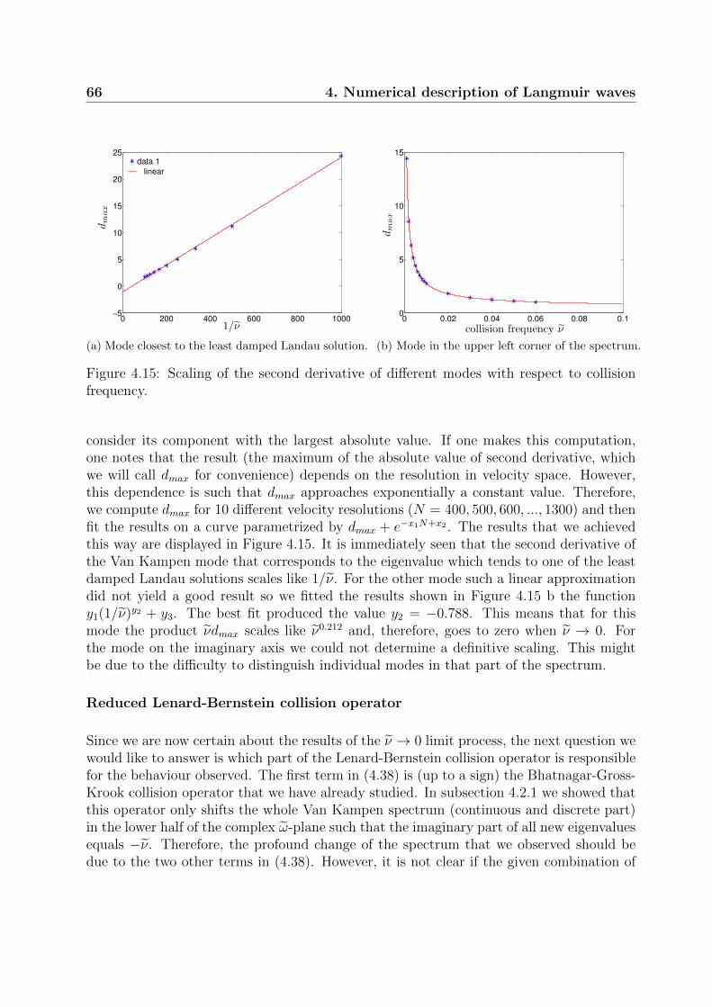
66 4. Numerical description of Langmuir waves
0 200 400 600 800 1000−5
0
5
10
15
20
25
1/ν
dm
ax
data 1
linear
(a) Mode closest to the least damped Landau solution.
0 0.02 0.04 0.06 0.08 0.10
5
10
15
collision frequency ν
dm
ax
(b) Mode in the upper left corner of the spectrum.
Figure 4.15: Scaling of the second derivative of different modes with respect to collisionfrequency.
consider its component with the largest absolute value. If one makes this computation,one notes that the result (the maximum of the absolute value of second derivative, whichwe will call dmax for convenience) depends on the resolution in velocity space. However,this dependence is such that dmax approaches exponentially a constant value. Therefore,we compute dmax for 10 different velocity resolutions (N = 400, 500, 600, ..., 1300) and thenfit the results on a curve parametrized by dmax + e−x1N+x2 . The results that we achievedthis way are displayed in Figure 4.15. It is immediately seen that the second derivative ofthe Van Kampen mode that corresponds to the eigenvalue which tends to one of the leastdamped Landau solutions scales like 1/ν. For the other mode such a linear approximationdid not yield a good result so we fitted the results shown in Figure 4.15 b the functiony1(1/ν)y2 + y3. The best fit produced the value y2 = −0.788. This means that for thismode the product νdmax scales like ν0.212 and, therefore, goes to zero when ν → 0. Forthe mode on the imaginary axis we could not determine a definitive scaling. This mightbe due to the difficulty to distinguish individual modes in that part of the spectrum.
Reduced Lenard-Bernstein collision operator
Since we are now certain about the results of the ν → 0 limit process, the next question wewould like to answer is which part of the Lenard-Bernstein collision operator is responsiblefor the behaviour observed. The first term in (4.38) is (up to a sign) the Bhatnagar-Gross-Krook collision operator that we have already studied. In subsection 4.2.1 we showed thatthis operator only shifts the whole Van Kampen spectrum (continuous and discrete part)in the lower half of the complex ω-plane such that the imaginary part of all new eigenvaluesequals −ν. Therefore, the profound change of the spectrum that we observed should bedue to the two other terms in (4.38). However, it is not clear if the given combination of

4.2 Introducing collision operators 67
both terms is necessary to produce such a behaviour of the spectrum in the ν → 0 limit orif only one of these terms plays an essential role. Our presumption is that the third partof the collision operator, the one involving a second derivative with respect to velocity, isresponsible for the abrupt change of the spectrum. In order to test this hypothesis, weremove the second term in (4.38). The discretized version of this reduced Lenard-Bernsteincollision operator is given by a matrix (denoted by Mν,2) similar to Mν that reads
Mν,2 := M + iν
(I +
1
∆v2(X+1 − 2I +X−1)
). (4.50)
The MATLAB routine that computes and plots the eigenvalues of Mν,2 can be found inthe Appendix under the name Lenard Bernstein 2. With it one can produce analogousplots to those in Figure 4.11. This way one sees that the spectrum of Mν,2 shows thesame qualitative behaviour as the one of the full matrix Mν , and this observation is a hintthat our conjecture was correct. In order to verify this, we focus on the part of the VanKampen spectrum that lies in the vicinity of the collisionless Landau roots. Computing thespectrum of Mν,2 for different collision frequencies and resolutions in velocity space, onecan note that in this case convergence of the spectrum is achieved at lower resolution thanwith Mν . For a collision frequency of 0.01, the spectrum converges already for 501 pointson the velocity axis. In Figure 4.16 we show the spectrum of Mν,2 for two different valuesof the collision frequency but, for the ease of comparison, at the same velocity resolution.
−3 −2 −1 0 1 2 3−3
−2.5
−2
−1.5
−1
−0.5
0
Re(ω/ωpe)
Im(ω
/ωpe)
vmax = 4vth; ν = 0.05ωpe ;N = 500
(a) ν = 0.05
−3 −2 −1 0 1 2 3−3
−2.5
−2
−1.5
−1
−0.5
0
Re(ω/ωpe)
Im(ω
/ωpe)
vmax = 4vth; ν = 0.01ωpe ;N = 500
(b) ν = 0.01
Figure 4.16: Spectrum of Mν,2 for N = 500.
One notes that on the second plot we have two Van Kampen eigenvalues that are veryclose to the two least damped Landau roots which is what we have expected. However,compared to the previous case, this time not the first (viewed from the real line) VanKampen eigenvalue goes to the Landau root but the second one. In order to make thismore clear we show in Figure 4.17 the same part of the spectrum of Mν,2 for differentcollision frequencies. The resolution is kept fixed (N = 500) which means that the numberof eigenvalues in the whole spectrum is fixed. Therefore, any changes in the upper part of
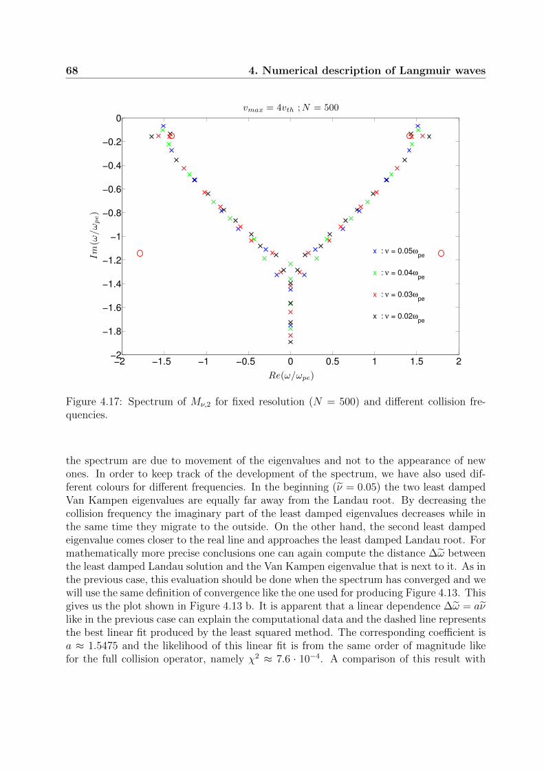
68 4. Numerical description of Langmuir waves
−2 −1.5 −1 −0.5 0 0.5 1 1.5 2−2
−1.8
−1.6
−1.4
−1.2
−1
−0.8
−0.6
−0.4
−0.2
0
Re(ω/ωpe)
Im(ω
/ωpe)
vmax = 4vth ;N = 500
x : ν = 0.05ωpe
x : ν = 0.04ωpe
x : ν = 0.03ωpe
x : ν = 0.02ωpe
Figure 4.17: Spectrum of Mν,2 for fixed resolution (N = 500) and different collision fre-quencies.
the spectrum are due to movement of the eigenvalues and not to the appearance of newones. In order to keep track of the development of the spectrum, we have also used dif-ferent colours for different frequencies. In the beginning (ν = 0.05) the two least dampedVan Kampen eigenvalues are equally far away from the Landau root. By decreasing thecollision frequency the imaginary part of the least damped eigenvalues decreases while inthe same time they migrate to the outside. On the other hand, the second least dampedeigenvalue comes closer to the real line and approaches the least damped Landau root. Formathematically more precise conclusions one can again compute the distance ∆ω betweenthe least damped Landau solution and the Van Kampen eigenvalue that is next to it. As inthe previous case, this evaluation should be done when the spectrum has converged and wewill use the same definition of convergence like the one used for producing Figure 4.13. Thisgives us the plot shown in Figure 4.13 b. It is apparent that a linear dependence ∆ω = aνlike in the previous case can explain the computational data and the dashed line representsthe best linear fit produced by the least squared method. The corresponding coefficient isa ≈ 1.5475 and the likelihood of this linear fit is from the same order of magnitude likefor the full collision operator, namely χ2 ≈ 7.6 · 10−4. A comparison of this result with

4.2 Introducing collision operators 69
the previous one shows that the Van Kampen eigenvalue still approaches the least dampedLandau solution but in this case the convergence is more than two times faster, i.e., thesecond term in (4.38), which we have excluded here, slows down the convergence of theVan Kampen eigenvalue but introduces no qualitative changes in the spectrum. However,one should also note that, in terms of absolute values, the full matrix Mν gives always asmaller ∆ω for the same velocity resolution and collision frequency (at least for the valuesthat we investigated).
Hermite polynomial representation
After we have seen the effect of collisions modelled via the Lenard-Bernstein collisionoperator in our numerical scheme we would like to make a small change of the numericalapproach. The previous analysis was inspired by [15]. However, in this work the authorsdo not discretize the velocity space. Instead, the perturbation is expanded in a separatefunctional basis and the coefficients of the expansion play the role of the isolated points invelocity space used in our numerical scheme. For the analysis that follows, we change thevelocity normalization and introduce the new variable u such that u := v/
√2. However, in
order to facilitate comparison with our previous results in the complex ω-plane we keep thenormalization of the frequency and wave number. With the new variable, (4.40) transformsinto
ωf1 =
√2ku
f1 +
√2
π
u
ke−u
2
+∞∫
−∞
f1(k, u′, ω)du+ iν
f1 + u
∂f1
∂u+
1
2
∂2 f1
∂u2
, (4.51)
where we have used the explicit form of the equilibrium distribution function rewritten in
the new coordinate. For the perturbationf1 we write the expansion
f1(k, u, ω) =
∞∑
n=0
an(k, ω)bn(u). (4.52)
For this expansion to be applicable, the perturbation should belong to a separable func-tional space over R in which the set of functions {bn(u)} forms a complete basis. We follow[15] and choose as basis vectors
bn(u) = Hn(u)e−u2
, (4.53)
where Hn(u) denotes the normalized nth Hermite polynomial defined as
Hn(u) :=(−1)n√2nn!√πeu
2 dne−u2
dun. (4.54)
One should note that the vectors of the basis {bn(u)} are neither orthogonal to each othernor do they have the same norm. In this notation we have that
70 4. Numerical description of Langmuir waves
+∞∫
−∞
Hn(u)Hm(u)e−u2
du = δmn ;dHn(u)
du=√
2nHn−1(u) , (4.55)
√2uHn(u) =
√n+ 1Hn+1(u) +
√nHn−1(u). (4.56)
The strategy when working with such an expansion is to use the properties (4.55) in such
a way that the sum in every term is the same (e.g., from n = 0 to ∞), and Hn(u)e−u2
appears in every term so it can be factored out. The equation that is left in the bracketsgives the connection between different coefficients an. This procedure for the first andthe collision term is straightforward, therefore we show only the calculation regarding thesecond expression on the right-hand side of (4.51). The integral gives
+∞∫
−∞
f1(k, u, ω)du =
∞∑
n=0
(−1)n√2nn!√πan(k, ω)
+∞∫
−∞
dne−u2
dundu =
=a0(k, ω)
4√π
+∞∫
−∞
e−u2
du
︸ ︷︷ ︸=√π
++∞∑
n=1
(−1)n√2nn!√πan(k, ω)
dn−1e−u2
dun−1
∣∣∣∣∣
+∞
−∞︸ ︷︷ ︸∝e−u2 |+∞−∞=0
= 4√πa0(k, ω). (4.57)
It is worth to make one side remark at this point. We could have chosen the basis vectorsbn as Hne
−u2/2. In that case the basis {bn} would have been orthonormal but then the
integral off1 over velocity would not have consisted of only one term proportional to a0
but it would have included contributions from all coefficients an with even index n and thiswould have made the further analysis more cumbersome. In this case the second term in(4.51) is
√2
π
u
ke−u
2
+∞∫
−∞
f1(k, u′, ω)du′ =
1
k
∞∑
n=0
an−1(k, ω)δ1nHn(u)e−u2
(4.58)
and the recursion relation between the coefficients reads
(k√n+
1
kδ1n
)an−1 + k
√n+ 1an+1 − inνan = ωan. (4.59)
One way to evaluate (4.59) and find the set of eigenfrequencies is to write it as a matrixeigenvalue equation in the form

4.2 Introducing collision operators 71
k
0 1 0 0 · · · 0 · · ·1 + 1
k20√
2 0 · · · 0 · · ·0
√2 0
√3 · · · 0 · · ·
0 0√
3 0 · · · 0 · · ·...
......
......
− iν
0 0 0 0 · · ·0 1 0 0 · · ·0 0 2 0 · · ·0 0 0 3 · · ·...
......
.... . .
·
a0
a1
a2
a3...
= ω
a0
a1
a2
a3...
.
(4.60)For a practical computation, of course, one has to cut the infinite matrices in (4.60) atsome point. However, the matrix elements in the equation above get bigger with increas-ing the number of the corresponding row or column. As also noted in [15], this feature ofthe matrix leads to problems with convergence of the solutions derived by this approach.Nevertheless, we will evaluate (4.59) in this way and use the same ideas as for our previousdiscretization scheme in order to determine wich part of the spectrum is converged andcan therefore be trusted.
−25 −20 −15 −10 −5 0 5 10 15 20 25−5
−4.5
−4
−3.5
−3
−2.5
−2
−1.5
−1
−0.5
0
Re(ω)/ωpe
Im(ω
)/ωpe
n = 500 ; ν/ωpe = 0.01 ; kλD = 0.5
(a) N = 500
−50 −40 −30 −20 −10 0 10 20 30 40 50−20
−18
−16
−14
−12
−10
−8
−6
−4
−2
0
Re(ω)/ωpe
Im(ω
)/ωpe
n = 2000 ; ν/ωpe = 0.01 ; kλD = 0.5
(b) N = 2000
Figure 4.18: Van Kampen spectrum in the Hermite polynomial representation for fixedcollision frequency (ν = 0.01) and different number of polynomials.
In Figure 4.18 we have show the Van Kampen spectrum for fixed collision frequency (ν =0.01) and different resolution in the space of Hermite polynomials. (High resolution meanshere that polynomials up to high n have been considered.) One sees that in this casethere is also an area of stochasticity in the middle of the spectrum where the Van Kampeneigenvalues do not adhere to the analytic symmetry of the equation. However, even for highn (at least up to n = 2000) this area does not shrink into a line situated on the imaginaryaxis. With the discretization in velocity space a line of Van Kampen eigenvalues formedthat was near the real line. In the Hermite polynomial representation these eigenvalues aremissing which might be due to the fact that they were not physical but rather a remnantof the velocity grid.
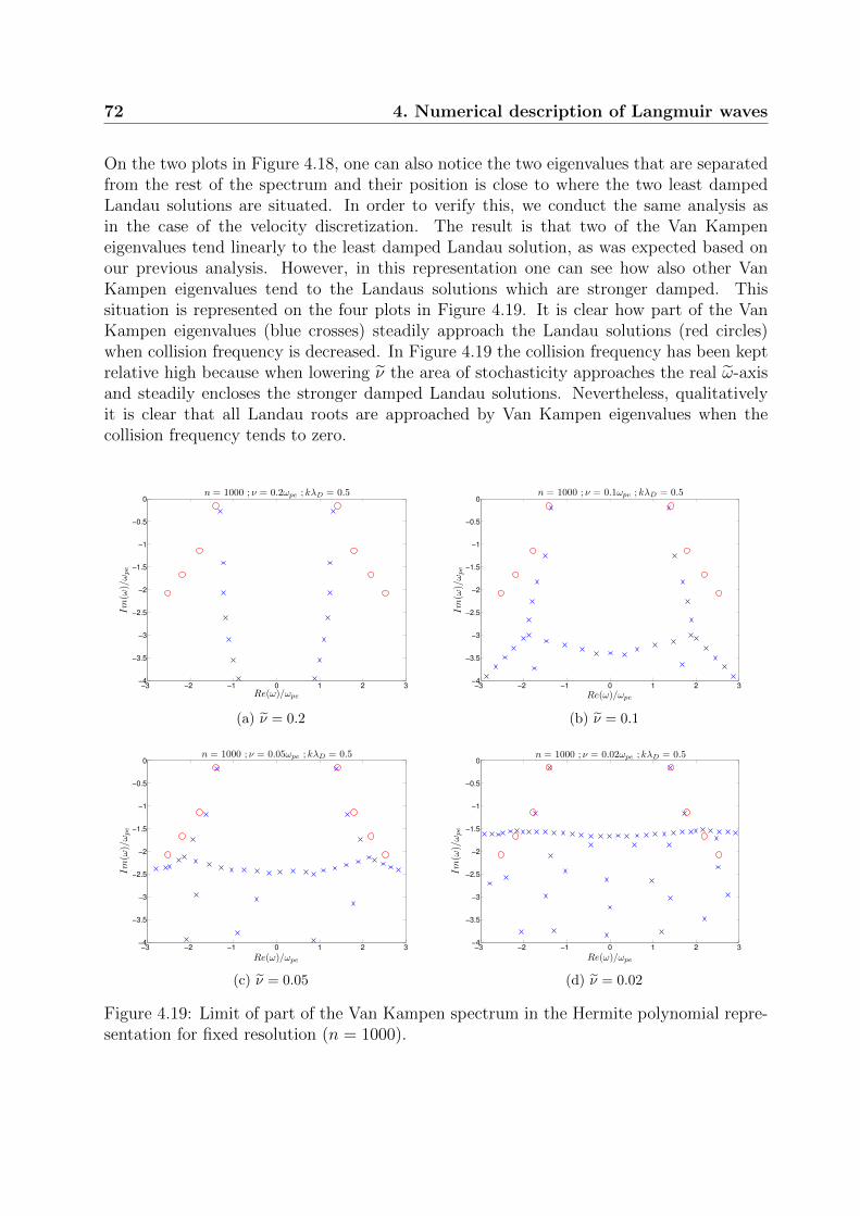
72 4. Numerical description of Langmuir waves
On the two plots in Figure 4.18, one can also notice the two eigenvalues that are separatedfrom the rest of the spectrum and their position is close to where the two least dampedLandau solutions are situated. In order to verify this, we conduct the same analysis asin the case of the velocity discretization. The result is that two of the Van Kampeneigenvalues tend linearly to the least damped Landau solution, as was expected based onour previous analysis. However, in this representation one can see how also other VanKampen eigenvalues tend to the Landaus solutions which are stronger damped. Thissituation is represented on the four plots in Figure 4.19. It is clear how part of the VanKampen eigenvalues (blue crosses) steadily approach the Landau solutions (red circles)when collision frequency is decreased. In Figure 4.19 the collision frequency has been keptrelative high because when lowering ν the area of stochasticity approaches the real ω-axisand steadily encloses the stronger damped Landau solutions. Nevertheless, qualitativelyit is clear that all Landau roots are approached by Van Kampen eigenvalues when thecollision frequency tends to zero.
−3 −2 −1 0 1 2 3−4
−3.5
−3
−2.5
−2
−1.5
−1
−0.5
0
Re(ω)/ωpe
Im(ω
)/ωpe
n = 1000 ; ν = 0.2ωpe ; kλD = 0.5
(a) ν = 0.2
−3 −2 −1 0 1 2 3−4
−3.5
−3
−2.5
−2
−1.5
−1
−0.5
0
Re(ω)/ωpe
Im(ω
)/ωpe
n = 1000 ; ν = 0.1ωpe ; kλD = 0.5
(b) ν = 0.1
−3 −2 −1 0 1 2 3−4
−3.5
−3
−2.5
−2
−1.5
−1
−0.5
0
Re(ω)/ωpe
Im(ω
)/ωpe
n = 1000 ; ν = 0.05ωpe ; kλD = 0.5
(c) ν = 0.05
−3 −2 −1 0 1 2 3−4
−3.5
−3
−2.5
−2
−1.5
−1
−0.5
0
Re(ω)/ωpe
Im(ω
)/ωpe
n = 1000 ; ν = 0.02ωpe ; kλD = 0.5
(d) ν = 0.02
Figure 4.19: Limit of part of the Van Kampen spectrum in the Hermite polynomial repre-sentation for fixed resolution (n = 1000).
Chapter 5
Extension to ion temperaturegradient (ITG) modes
In this chapter we shall discuss some consequences of temperature and density gradientsin the framework of drift-kinetics. After introducing the physics of the slab ITG modeland deriving a few analytical results, a numerical evaluation of the equations follows. Weconsider again first the collisionfree case and then introduce collisions into the system viathe Lenard-Bernstein collision operator.
5.1 The slab ITG model
Our starting point in this chapter will be the drift-kinetic equation used extensively inplasma physics. For the derivation of this equation we follow [3]. First, let us assume thatwe have a strongly magnetized plasma and a constant (in time as well as in space) magnetic
field ~B = B~ez in the z-direction. In this case, the particles (ions and electrons) gyraterapidly around the field lines and are effectively bound to them while being able to movefreely along the field lines. As long as one is only interested in low-frequency dynamics, onecan average out the phase dependence of the rapid gyromotion and thus reduce the velocityspace of the particles by one dimension. If fi,gc(~r,~v, t) denotes the distribution function ofion gyrocentres, one can write that fi,gc(~r,~v, t) → fi,gc(~r, v||, v⊥, t). From now on we willsuppress for the ease of notation the subscript gc. This reduction of the six-dimensionalphase space is called ‘gyro-kinetic approximation’. However, here we also neglect finiteLarmor radius (FLR) effects which is not done in gyro-kinetics. Therefore, one shouldcall the approximative model used here drift-kinetics. In mathematical terms, we haveintroduced cylindrical coordinates in velocity space and have integrated out the angledependence such that now the volume element in velocity space is given by 2πv⊥dv⊥dv||.If the number of particles remains constant, then in analogy with the usual kinetic theoryone can write that
74 5. Extension to ion temperature gradient (ITG) modes
0 =∂fi∂t
+∇(5) · (~ufi) =∂fi∂t
+∇ · (~rfi) +1
v⊥
∂
∂v⊥(v⊥v⊥fi) +
∂
∂v||(v||fi), (5.1)
where∇(5) denotes a divergence in the five dimensional phase space with cylindrical velocitycoordinates and the five-dimensional vector ~u is defined as ~u := (~r, v⊥, v||). The velocity v⊥perpendicular to the magnetic field is usually much smaller than the parallel velocity v||.Since our primary goal is to gain a qualitative understanding of this model, we consideronly first order effects, which in this case is the ~E × ~B drift. With this approximation thevelocity reads
~r = ~vD + v||~ez, (5.2)
where ~vD = ~E × ~B/B2. Using this expression for the drift velocity and the fact that themagnetic field is constant, one can easily show that ∇ · ~vD = 0. The gyromotion of theions is related to the magnetic moment which is given by µ = miv
2⊥/(2B), where mi is the
ion mass. In a magnetic field that is constant in space and in time, this magnetic momentis also constant and, therefore, v⊥ = 0. According to the second Newton’s law, the timederivative of v|| equals the force acting on the ion that is parallel to the magnetic fielddivided by its mass. The force of the magnetic field has no component that is tangent toit, so in the z-direction the only contribution comes from the z-component of the electricfield, i.e., v|| = eE||/mi. Using these results in (5.1), one arrives at
∂fi∂t
+(~v|| + ~vD
)· ∇fi +
e
mi
E||∂fi∂v||
= 0. (5.3)
Since the drift velocity is much smaller than the parallel velocity, one can neglect the v⊥-dependence of fi. Setting ∂B
∂t= 0 means that we can express the electric field as ~E = −∇ϕ,
where ϕ is the electrostatic potential. Subsequently, we are going to introduce gradientsof the equilibrium temperature and density which we take for simplicity in the x direction.In order to circumvent unnecessary mathematical complications arising from the Fouriertransformation in y and z of the approximate drift kinetic equation, we consider an elec-trostatic potential which is a function only of y, z and t: ϕ = ϕ (y, z, t). This assumptionimplies also the same dependency of the electric field and that Ex = 0. Strictly speaking,we can consider also an electric field with a non-vanishing component in x-direction. How-ever, this is not going to influence the model qualitatively and, therefore, we take Ex to bezero. In physical terms this is equivalent to setting kx to zero.
At this point, we interrupt the exact quantitative description of the slab ITG model andgive a more physical explanation of the ITG instability with the help of the simple pictureshown in Figure 5.1 which represents the geometry of our model. Although this expla-nation comes from fluid theory, it will still be useful to gain some physical insight. Weare not going to present the fluid equations here but merely adopt the results derived in[20]. Assume that the temperature gradient points in the positive x-direction and that awavelike ion density perturbation is formed in the plasma with a maximum at x = y = 0.

5.1 The slab ITG model 75
Figure 5.1: Simplified picture of the ITG instability (source: Cowley et. al., Phys. Fluids1991).
This instantaneously induces an electric field towards the the origin of the coordinate sys-tem. Together with the magnetic field, this electric field gives rise to a ~E × ~B drift thatin this situation is parallel to the temperature gradient, as shown in the figure, i.e., thisdrift brings plasma from the cold to the hot areas. The effect of this advection of colderplasma is that it cools the perturbation and thus decreases its pressure which, however,causes a flow of ions into the perturbation, since the pressure there is lower. This feedbackmechanism leads to a growth of this perturbation in the ion density, i.e., an instability.If one does the corresponding calculation, then one sees that there is a slight phase shiftbetween the quantities involved. The ~E × ~B drift does not peak at y = 0 where the maxi-mum of the ion density perturbations. Since the drift ‘feeds’ the perturbation, this phaseshift leads to a movement of the instability in the plasma.
Now we continue with the description of the kinetic slab ITG model. In order to approxi-mate (5.3), we will use the same linearisation procedure as in the previous chapter. So wewrite
fi(~r, v||, t) = f0i(x, v||) + f1i(~r, v||, t), (5.4)
where the subscripts 0 and 1 denote the equilibrium and the perturbation of the distributionfunction of gyrocentres. The only difference here is that we will allow for f0i to depend onone of the spatial coordinates, namely the same coordinate on which also the temperatureand density depend. It should be noted that the electric field arises due to the perturbation.
76 5. Extension to ion temperature gradient (ITG) modes
Since the drift velocity is proportional to the electric field, we will consider it to be also afirst order quantity. Substituting the last expression for fi into (5.3) and neglecting secondorder terms we arrive at
∂f1i
∂t+ v||
∂f1i
∂z− ∂ϕ
∂y
1
B
∂f0i
∂x− e
mi
∂ϕ
∂z
∂f0i
∂x= 0. (5.5)
For the derivation of the last equation one should take into account that
~E × ~B = −∇ϕ(y, z, t)× ~B = −∂ϕ∂yB~ex and E|| := −
∂ϕ
∂z. (5.6)
In order to get a self consistent equation determining f1i, we need a relation between theelectrostatic potential ϕ and f1i. Similar to the MHD case, we can assume some equation ofstate which gives us self-consistency. Since the ion mass is much greater than the electronmass, the average electron velocity is much higher than the average ion velocity when bothelectron and ion temperatures are nearly the same. In physical terms this means thatthe electrons react on the potential differences, caused by f1i, on time scales much fasterthan the time scales on which f1i and therefore the electrostatic potential changes, i.e., wesay that the electrons are adiabatic. Mathematically, this means that at every momentof time, the electrons will have a linearised Boltzmann distribution corresponding to theelectrostatic potential ϕ(y, z, t) they experience:
n1e(~r, t) = n0e(x)eϕ(y, z, t)
kBTe(x), (5.7)
where n1e and n0e are the perturbed and equilibrium electron densities respectively andTe is the electron temperature which can also vary in x. Using the quasi-neutrality of theplasma (here the ions have the charge e), namely that
n0i(x) = noe(x) and n1e(~r, t) = n1i(~r, t) :=
+∞∫
−∞
f1i(~r, v||, t)dv||, (5.8)
we derive the desired connection between f1i and the electrostatic potential which reads
ϕ(y, z, t) =kBTe(x)
en0i(x)
+∞∫
−∞
f1i(~r, v||, t)dv||. (5.9)
In order to work with (5.5) in a more comfortable way (especially in the case of a numericalanalysis), it is convenient to normalize the quantities in the equation. Since the densitiesand temperatures are continuous functions of space, we will normalize them over theirmaximal values:
T(m)i,e := sup {Ti,e(x)} ; n(m) := sup {n0i(x)} = sup {n0e(x)} . (5.10)
Given these definitions, we can now define a typical ion thermal velocity given by

5.1 The slab ITG model 77
vth,i :=
√kBT
(m)i
mi
. (5.11)
One should also note that there are different spatial scales in this problem. For stronglymagnetized plasmas the mean free path of the particles along the magnetic field is large, soall plasma quantities vary slowly in the z-direction. The equilibrium distribution functionf0i also experiences considerable changes over a scale length comparable to the length ofthe system (which we call a). Therefore spatial derivatives of f0i and derivatives withrespect to z will be normalized with respect to a.1 Perpendicular to the magnetic fieldthe movement of particles is bound by their gyromotion, so it is physically meaningful tonormalize derivatives of the perturbed quantities with respect to x or y over the Larmorradius of a particle whose velocity perpendicular to the magnetic field equals vth,i, i.e.,
rL :=
√kBT
(m)i mi
eB. (5.12)
The time scales of interest are set by the ion gyro-frequency ωg of the particles which interms of magnetic field and particle properties is given by
ωg =eB
mi
=vth,irL
. (5.13)
One should notice that ωg does not depend on the particle energy (at least for non-relativistic energies) and is therefore the same for all ions. We can now define the nor-malized quantities (denoted by a tilde over the corresponding letter) we will work withvia:
f1,0i :=vth,in(m)
f1,0i ; t := tωg ; v|| :=v||vth,i
; ϕ :=e
kBT(m)i
ϕ. (5.14)
Using these definitions, one can transform (5.5) and arrives at
1
ρ∗
∂f1i
∂t+ v||
∂f1i
∂z− ∂ϕ
∂y
∂f0i
∂x− ∂ϕ
∂z
∂f0i
∂x= 0, (5.15)
where ρ∗ is the ratio between the Larmor radius, rL, and a, the system length in perpen-dicular direction. In order to simplify (5.15) we Fourier transform it with respect to z, yand t according to the convention
g(z, y, t) =1
(2π)3/2
+∞∫
−∞
+∞∫
−∞
+∞∫
−∞
g(k||, ky, ω)e−ik||ze−iky yeiωtdkydk||dω. (5.16)
1Strictly speaking the mean free path of a particle in a typical tokamak is a few kilometres whichexceeds the system length by three orders of magnitude. However, from a mathematical point of viewthere is nothing wrong in normalizing the derivatives w.r.t. z over a and later on such a normalizationwill turn out to be useful.
78 5. Extension to ion temperature gradient (ITG) modes
Furthermore, we will assume that the equilibrium distribution f0i is a local Maxwell dis-tribution in which the equilibrium density and temperature vary with x, i.e.,
f0i(x, v||) =n0i(x)√
2πkBTi(x)/mi
exp
(−
miv2||
2kBTi(x)
). (5.17)
Normalizing this expression with respect to the aforementioned quantities gives
f0i(x, v||) =n0i(x)√2πTi(x)
exp
(−1
2
v2||
Ti(x)
), (5.18)
where we have normalized the temperature via Ti,e(x) := Ti,e(x)/T(m)i . From this follows
immediately that ∂f0i/∂v|| = (v||/Ti)f0i. Substituting this, after Fourier transforming(5.15), leads to
(ω
ρ∗− k||v||
)f 1,i +
(ky∂f0i
∂x− k||v||
Ti(x)f0i
)ϕ = 0. (5.19)
The relation between ϕ andf 1,i is derived by normalizing and Fourier-transforming (5.9):
ϕ =τ (m)Te(x)
n0i(x)
+∞∫
−∞
f1i(..., v||, ...)dv||, (5.20)
where τ (m) is given by the ratio T(m)e /T
(m)i . The only parameters in f0i which depend on x
are density and temperature, so using (5.18) we can easily express the derivative ∂f0i/∂xthrough the gradients of temperature and density. A straightforward calculation gives
ky∂f0i
∂x− k||v||
Ti(x)f0i =
(−1
2
ky
Ti(x)
dTi(x)
dx+
1
2
kyv2||
T 2i (x)
dTi(x)
dx+
kyn0,i(x)
dn0i(x)
dx−
− k||v||Ti(x)
)f0i(x, v||) =: α(x, v||)f0i(x, v||). (5.21)
Combining this expression with (5.20) and substitution in (5.19) yields
ω
ρ∗
f 1i = k||v||
f 1i−
τ (m)Te(x)
n0i(x)α(x, v||)f0i(x, v||)
︸ ︷︷ ︸=ψ(x,v||)
+∞∫
−∞
f 1i(..., v
′||, ...)dv
′||. (5.22)
One can view this equation as an eigenvalue equation of a linear operator acting onf 1i,
where the eigenvalues this time are denoted by ω/ρ∗. If one compares (5.22) with (3.1), it
5.1 The slab ITG model 79
becomes immediately apparent that this is qualitatively the same operator that we studiedin chapter 3. The only difference with respect to the case of Langmuir waves is that nowthe explicit form of the function ψ(v) is more complicated. However, this is not going to bea problem here, since in chapter 3 we investigated the properties and the spectrum of thisoperator without specifying the exact form of ψ(v). We only assumed that it belongs to thespace H which is also the case in (5.22). We derived that this operator has a spectrum thatconsists of a continuous part situated on the entire real line and a discrete part that obeysthe condition (3.16), where the integral is to be understood in the sense of the Cauchyprinciple value. We also agreed on the prescription that, if the integral is done along theLandau contour, then this condition gives the corresponding Landau solutions. Here thisleads to
1− τ (m)Te(x)
n0i(x)k||
∫
L
α(x, v||)f0i(x, v||)
v|| − ωL/(k||ρ∗)dv|| = 0. (5.23)
Before further transforming (5.23), it is useful to note some relations between the integralsone encounters in this equation and the plasma dispersion function Z. Using the definitionof Z given in [1] one can derive2 the following expressions:
∫
L
e−bx2
x− adx =√πZ(a
√b) ;
∫
L
xe−bx2
x− a dx =
√π
b+ a√πZ(a
√b) ;
∫
L
x2e−bx2
x− a dx = a
√π
b+ a2√πZ(a
√b),
(5.24)
where a ∈ C and b ∈ R+ are fixed parameters. In the expression for α(x, v||) one encountersgradients of the ion temperature and equilibrium density. For ease of notation we define
d ln Ti(x)
dx:= − 1
LT (x)and
d ln n0i(x)
dx:= − 1
Ln(x), (5.25)
where LT and Ln have the physical dimension of length and are normalized over the typicalsystem length a. The usefulness of the definitions above will become clear later on. Withthese definitions and the explicit form of α(x, v||) given in (5.21) we can now express (5.23)in way that involves the plasma dispersion function and is more convenient for numericalanalysis, namely
2The exact derivation is shown in the Appendix.

80 5. Extension to ion temperature gradient (ITG) modes
1+τ (m) Te(x)
Ti(x)+τ (m) Te(x)
2Ti(x)
ky
k||
1
LT (x)
(ω
ρ∗k||
)+τ (m)Z
ω√
2Ti(x)ρ∗k||
·[
Te(x)√2T
3/2i (x)
(ω
ρ∗k||
)+
+Te(x)√2Ti(x)
ky
k||
(1
Ln(x)− 1
2
1
LT (x)
)+
Te(x)√2T
3/2i (x)
ky
k||
1
LT (x)
(ω√
2ρ∗k||
)2 = 0. (5.26)
The special case of a plasma in a global thermal equilibrium with homogeneous equilibriumion density is derived in this approximated model by taking the limit LT → +∞ andLn → +∞. This leads to
1 + τ (m) + τ (m)
(ω√
2ρ∗k||
)Z
(ω√
2ρ∗k||
)= 0, (5.27)
which one recognises as the dispersion relation of ion acoustic waves in a strongly magne-tized plasma.In our further analysis we are going to work with a commonly used approximation forthe temperature and density gradients. In this model, one considers small volumes in theplasma such that it can be assumed that both temperature and density vary only weaklyover the distances under consideration, so we set Ti(x) = Te(x) = ni(x) = 1. However, wedo not want to neglect the gradients entirely and, therefore, approximate them by takingLT and Ln to be constant but finite. The physical meaning of the quantities LT and Lnis that they represent the length scales over which temperature and density vary consider-ably. Since these length scales are usually considerably bigger than the Larmor radius andof the same order of magnitude as the perpendicular system length a, they are normalizedwith respect to a. With this approximation the dispersion relation reads
1 + τ (m) + τ (m) ky
k||
1
2LT
(ωL
ρ∗k||
)+ τ (m)Z
(ωL√2ρ∗k||
)·[
ky
k||√
2
(1
Ln− 1
2
1
LT
)+
+ωL
ρ∗k||√
2+
ky
k||√
2
1
LT
(ωL√2ρ∗k||
)2 = 0, (5.28)
where we have denoted the solutions of this equation by ωL in order to keep in mind thatthey arise when one integrates along the Landau contour in order to avoid ambiguity in theintegral in (5.23). We can avoid the ambiguity also by taking the Cauchy principal valueof the integral and, as we saw in chapter 3, this treatment would give us the discrete partof the Van Kampen spectrum. Therefore, these Van Kampen eigenfrequencies, denotedhere by ωV , fulfil the equation

5.1 The slab ITG model 81
1− τ (m)Te(x)
n0i(x)k||p.v.
+∞∫
−∞
α(x, v||)f0i(x, v||)
v|| − ωV /(k||ρ∗)dv|| = 0, (5.29)
which is analogous to (5.23). The situation here is similar to the one we already investigatedin subsection 4.1.2. By comparing (5.23) and (5.29) and recalling the definition of theLandau contour we immediately conclude that, if one of them has a solution with a positiveimaginary part, then it is also a solution to the second equation, since for poles in the upperhalf of the complex ω-plane the Landau contour reduces to a simple integration along thereal line as also the Cauchy principal value. In analogy to 4.1.2, we would like to saysomething about the symmetry of the discrete part of the Van Kampen spectrum. Byusing the definition of α(x, v||) and the explicit form of f0,i(x, v) one can split the integralin (5.29), which for ease of notation we denote here as the function g(a), into a sum ofthree terms, namely
g(a) =n0,i(x)ky√
2πTi(x)
(− 1
Ln(x)+
1
2LT (x)
)p.v.
+∞∫
−∞
e−bt2
t− adt−
− n0,i(x)ky
2Ti(x)LT (x)
√2πTi(x)
p.v.
+∞∫
−∞
t2e−bt2
t− a dt−n0,i(x)k||
Ti(x)
√2πTi(x)
p.v.
+∞∫
−∞
te−bt2
t− a dt, (5.30)
where we have introduced the substitutions t := v||, a := ωV /(ρ∗k||) and b := 1/(2Ti(x)).For a non-vanishing imaginary part of a we can split these three integrals into real andimaginary in the same way as we proceeded in subsection 4.1.2. This gives
Re(g(a)) =n0,i(x)√2πTi(x)
−ky
2Ti(x)LT (x)
+∞∫
−∞
t2(t− ar)e−bt2
|t− a|2 dt− k||
Ti(x)
+∞∫
−∞
t(t− ar)e−bt2
|t− a|2 dt+
+ky
(−1
Ln(x)+
1
2LT (x)
) +∞∫
−∞
(t− ar)e−bt2
|t− a|2 dt
(5.31)
and
Im(g(a)) = ain0,i(x)√2πTi(x)
−ky
2Ti(x)LT (x)
+∞∫
−∞
t2e−bt2
|t− a|2dt−k||
Ti(x)
+∞∫
−∞
te−bt2
|t− a|2dt+
+ky
(−1
Ln(x)+
1
2LT (x)
) +∞∫
−∞
e−bt2
|t− a|2dt
(5.32)
82 5. Extension to ion temperature gradient (ITG) modes
From this decomposition follows that Re(g(a∗)) = Re(g(a)) and Im(g(a∗)) = −Im(g(a)),which is equivalent to g∗(a) = g(a∗). In terms of the function g, (5.29) reads
1− τ (m)Te(x)
n0i(x)k||g
(ωV
ρ∗k||
)= 0. (5.33)
When we take the complex conjugate of both side of this equation and use the property ofg, that we just derived, we see that
1− τ (m)Te(x)
n0i(x)k||g
(ω∗V
ρ∗k||
)= 0, (5.34)
i.e., if ωV is a solution of (5.29), then so is also its complex conjugate. Since, the otherpart of the Van Kampen spectrum lies on the real line, then the same symmetry appliesto every eigenvalue. We summarize our conclusions as follows:
• The Van Kampen spectrum possesses a mirror symmetry with respect to the realω-axis.
• The Van Kampen eigenvalues with positive imaginary part (i.e., unstable) are alsoLandau solutions.
One should note that the above properties of the Van Kampen spectrum and the set ofLandau solutions does not depend on the gradient approximations we introduced and,therefore, hold for arbitrary functions Ti(x), Te(x) and n0,i(x).
The equations in this subsection are even more complicated than those that we had before,so in order to gain more insights into this model, we have to solve them numerically. Forthis we use the same numerical scheme as before, namely we discretize the v||-axis andconsider only a finite interval on it that is symmetric with respect to zero. At this point,we go to the approximation that was already introduced, namely
Ti(x) ≡ 1 ; Te(x) ≡ 1 ; n0,i(x) ≡ 1 ; LT (x) = const ; Ln(x) = const. (5.35)
In this framework our model has six parameters: ky, k||, ρ∗, τ(m), LT and Ln which we are
allowed to choose freely.
5.2 Numerical description of collisionless ITG modes
The way we implement the discretization in velocity space follows the same scheme as inthe case of Langmuir waves: we approximate the continuous operator on the right-handside of (5.22) with a matrix the rank of which equals the number of velocity points. The
only difference here is the explicit form of the vector ~G, namely we now have

5.2 Numerical description of collisionless ITG modes 83
Gj =τ (m)ky√
2π
(1
2LT− 1
Ln− k||
kyv||,j −
v2||,j
2LT
)e−v
2||,j/2. (5.36)
The Van Kampen approach reduces again to finding the eigenvalues of the matrix thatcorresponds to the continuous operator, and in the slab ITG model this matrix is alsodefined via equation (4.9). For finding the positions of the Landau solutions we proceed inthe same way as in section 2.2 and draw a contour plot of the absolute value of the functionon the right hand side of (5.28). The combined results of both approaches are shown inFigure 5.2 where the Van Kampen eigenvalues are denoted by blue crosses. One noticesthat there is only one unstable Van Kampen eigenvalue and one unstable Landau solutionand their positions in the complex ω-plane are the same. This is also what we expectedfrom our mathematical analysis. The Van Kampen spectrum has the mirror symmetrywith respect to the real axis that we derived. In the case of Langmuir waves, the set ofLandau solutions was symmetric with respect to the imaginary axis. Here, this symmetryis broken because of the gradients that set a preferable direction in space.
−2 −1.5 −1 −0.5 0 0.5 1 1.5 2−1
−0.8
−0.6
−0.4
−0.2
0
0.2
0.4
Re(ω/ωg)
Im(
ω/
ωg)
vmax
/vth = 6 ; ∆v/v
th = 0.06 ; L
T/a = 0.1; L
n/a = 1
Figure 5.2: Landau solutions and Van Kampen spectrum in the case of slab ITG fork|| = ky = 0.3 and ρ∗ = 1.
It is noteworthy that only the temperature gradient produces the instability. When in-troduced, a density gradient stabilizes the system, i.e., for a fixed LT decreasing Ln(that corresponds to an increase of the density gradient) lowers the growth rate of the

84 5. Extension to ion temperature gradient (ITG) modes
instability and if Ln falls below a certain threshold, the pair of one unstable and onedamped solution disappears and all Van Kampen eigenvalues lie on the real line. As ex-plained in [3], one can formulate this condition in mathematical terms. If the quantityΛ := (Ln/LT )(ky/kpar)
2(vD/vth,i)2 is large compared to one, then the threshold for an in-
stability is that ηi := Ln/LT > 2. Since vD/vth,i is of the order of rL/a, then in our unitsof normalization the parameter Λ is
Λ = ηi
(kyk||
)2(vDvth,i
)2
∼ ηi
(kyk||
)2 (rLa
)2
= ηi
(ky
k||
)2
which does not depend on ρ∗. If one sets the parameters of our program appropriately,e.g., ky = 0.3 and k|| = 0.03, then it reproduces this threshold. When dealing with the ITGinstability in the framework of gyrokinetics, one usually performs what is called a scan inthe perpendicular wave number, namely for fixed gradients and parallel wave number, kyis varied. This gives us the growth rate of the instability as a function of ky. In such scansone sees that the growth rate initially increases, peaks at some value of the perpendicularwave number and then decreases monotonically while it reaches zero for ky in the vicin-ity of one. Since the perpendicular wave number is normalized over the gyroradius, theeffect of rL being finite, that becomes prominent for ky > 1, stabilized the wave. In ourmodel we did not include finite gyroradius effects and, thus, such a scan with respect tothe perpendicular wave number shows a different picture, namely the growth rate of theinstability increases monotonically with ky.
In analogy to subsection 4.1.1, we investigate the density of eigenmodes (strictly speaking,the density of the projection of the eigenmodes onto the real ω-axis). One example thatcorresponds to the set of parameters of the previous plot is shown in Figure 5.3. The largespike is due to the fact that the real part of the frequency for the unstable and the dampedeigenvalue is the same, i.e., at this point ∆ω is zero. When the gradients are chosen suchthat there is no instability, then there is still a peak at that point that gets higher andsharper when the Ln increases and approaches the threshold for producing an instability.3
This suggests that in the stable case, two of the Van Kampen eigenvalues around thispoint approach each other until they have the same position. If one increases Ln further(or decreases LT ), then these eigenvalues separate again but this time in a direction per-pendicular to the real axis, i.e., they get a non-zero imaginary part and the pair of anunstable and a damped eigenmode is formed.The smaller peak in the spectral density, situated to the right of the big one, lies above theleast damped Landau solution shown on Figure 5.2. This indicates that also in the ITGmodel, the Van Kampen eigenvalues ‘sense’ the Landau solutions. The red dashed linecorresponds to the constant density of eigenvalues (at 1/k|| = 1/3) that comes from the
multiplication operator k||v|| in the first part of (5.22), i.e., the variations of the spectral
3When the condition ky � k|| is not met, there is still a threshold. However, it depends not only onthe ratio of the gradients but also on their explicit values.

5.2 Numerical description of collisionless ITG modes 85
−2 −1.5 −1 −0.5 0 0.5 1 1.5 23
3.2
3.4
3.6
3.8
4
4.2
4.4
4.6
4.8
5
Re(ω/ωg)
spectral density
vmax
/vth = 6 ; ∆v/v
th = 0.03 ; L
T/a = 0.1; L
n/a = 1
Figure 5.3: Density of the projection of the Van Kampen eigenvalues on the real line inthe case of slab ITG model for k|| = ky = 0.3 and ρ∗ = 1.
density are due to the second term in (5.22) that involves the electrostatic potential.One can also compute the coefficients when a given perturbation that evolves in time isdecomposed in the basis of Van Kampen modes. In this case the calculation in (4.16)still holds. However, if there is an instability, then its coefficient is going to grow in timeexponentially and dominate over the others.
It is useful to make a connection between the results derived here and those of other moresophisticated models. We will compare the Van Kampen spectrum from our model withthose achieved with the gyrokinetic simulation code GENE. This abbreviation stands for‘gyrokinetic electromagnetic numerical experiment’ and a description of the code can befound in [21] as well as at http://gene.rzg.mpg.de where also the entire code can be down-loaded. The applicability of GENE is much wider than the simple example presented here.It can treat plasmas in a variety of conditions that involve realistic geometries of the mag-netic field, perturbations of the magnetic field, finite Larmor radius effects, etc. In theframework of gyrokinetics, the ion distribution function is defined in a five dimensionalphase space, since the velocity space is reduced by one dimension and only the parallelvelocity and the energy of the gyromotion (proportional to the magnetic moment µ of thegyrating particle) are left. The distribution of both variables is similar to a Maxwellian,i.e., for |v|||, µ → ∞ it falls rapidly to zero. In slab geometry, the magnetic moment canbe factored and integrated out of the equations implemented in GENE. Then the program

86 5. Extension to ion temperature gradient (ITG) modes
−3 −2 −1 0 1 2 3
x 10−3
−12
−10
−8
−6
−4
−2
0
2
4x 10
−4
Re(ω)/ωg
Im(ω
)/ωg
v||,max/vth = 6 ;∆v||/vth = 0.06 ; LT = 0.25 ; Ln = 1
(a) Slab ITG model described in this work.
-0.03
-0.02
-0.01
0
0.01
0.02
0.03
-0.2 -0.15 -0.1 -0.05 0 0.05 0.1 0.15 0.2 0.25 0.3
γ/(v T
/R)
ω/(vT /R)
EV Spectrum
(b) GENE equivalent of the slab ITG.
Figure 5.4: Comparison of Van Kampen spectra between the slab ITG model describedin this work and the equivalent problem solved with GENE; k|| = 0.03, ky = 0.3 andρ∗ = 0.01.
solves almost the same set of equations. The only difference is that in GENE there is noFourier transformation with respect to k|| [27]. This issue was solved by David Hatch witha Fourier filter with respect to k|| for the modes. After this step, one can compare theresults of both approaches directly. Such a comparison is shown in Figure 5.4. The leftplot has been produced by the program drift eigenvalue.m and the right one has beenmade by David Hatch with GENE such that it corresponds to the same parameters. InFigure 5.4, the Van Kampen eigenvalues are denoted by blue crosses and also the eightLandau solutions that are closest to the real line are shown (red circles). The Van Kampeneigenvalues produced by GENE are represented by red pluses. The immediate compari-son between the two plots shows a good agreement which is not only qualitative but alsoquantitative. For example one could compare the position of the instability. Our programproduces an instability at ω ≈ (−0.82+2.6i) ·10−4 and GENE at ω ≈ (−0.87+2.6i) ·10−4.The discrepancy between the two results is small and it appears in the real part, so it isprobably due to the fact that one takes only a finite number of points in velocity space.It is also noteworthy that one of the real Van Kampen eigenvalues is separated from the rest.(Its position is the same on both plots.) This is due to the fact that this eigenvalue belongsto the discrete part of the Van Kampen spectrum that is defined as the set of solutions of(5.29). The length of the box in which the other eigenvalues are situated is directly related
to the length of the interval in velocity space that is used, namely ωmax = ρ∗kmaxv||,max.One can also easily compute the discrete Van Kampen eigenvalues directly by plotting theright-hand side of (5.29) and find the values of the argument for which this real valued func-tion gives zero. For the set of parameters used for producing Figure 5.4 there are in totalfour discrete Van Kampen eigenvalues, namely ωV,1 = −0.493 · 10−3, ωV,2 = −0.020 · 10−3,ωV,3 = 0.519 · 10−3 and ωV,4 = 3.171 · 10−3. The last of these four solutions equals exactly

5.2 Numerical description of collisionless ITG modes 87
the separated real eigenvalue that our program produced. This was not expected, since inour discretization scheme we approximated velocity integrations like in (5.29) with a finitesum that extends from −v||,max to v||,max. However, despite this fact, our matrix apparently‘knows’ something about the position of the discrete Van Kampen solutions, at least whenthey are outside the frequency ‘box’ on the real line. In Figure 5.4(a) one sees that theone of the Landau solutions seems to have the same position as the discrete Van Kampeneigenvalue. In fact, it is very close to it but not at the same spot. The Van Kampenvalue is real, while the Landau solution has a small imaginary part of approximatively2.3 · 10−8. Using an approximation of the plasma dispersion function for arguments witha small imaginary part, whose absolute value is much smaller than that of the real part ofthe argument, one can show that such solutions of (5.23) are almost solutions of (5.29).
It is also interesting to look at the mode structure of the numerical Van Kampen eigen-modes. First, we write down the analytical eigenfunctions. By the result (3.17) in chapter3 they read
fω(v||) =
τ (m)Te(x)
n0i(x)k||
α(x, v||)f0i(x, v||)
v|| − ω/(ρ∗k||)+
+ k||δ(k||v|| − ω)
1− τ (m)Te(x)
n0i(x)k||p.v.
+∞∫
−∞
α(x, v′||)f0i(x, v′||)
v′|| − ω/(k||ρ∗)dv′||
. (5.37)
For eigenmodes that correspond to the discrete part of the Van Kampen spectrum, thecoefficient in brackets after the delta function is zero, thus only the first part is left. If theeigenfrequency is complex, this first part has also no poles, since v|| and k|| are real.
−6 −4 −2 0 2 4 6−5
−4
−3
−2
−1
0
1
2
3
4
5
normalized velocity v||/vth,i
| f ω(v
||)|
v||,max/vth = 6 ;∆v||/vth = 0.06 ; LT = 0.25 ; Ln = 1
(a) Eigenmodes corresponding to the unstable,damped and the isolated real eigenvalue.
−6 −4 −2 0 2 4 6−200
−150
−100
−50
0
50
100
150
normalized velocity v||/vth,i
| f ω(v
||)|
v||,max/vth = 6 ;∆v||/vth = 0.06 ; LT = 0.25 ; Ln = 1
(b) Eigenmode corresponding to an eigenvalue fromthe continuum.
Figure 5.5: Mode structure of different numerical eigenvectors.
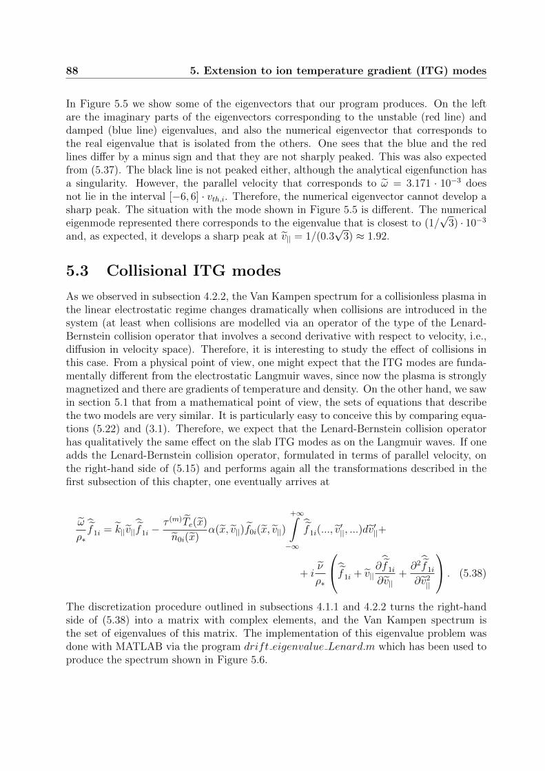
88 5. Extension to ion temperature gradient (ITG) modes
In Figure 5.5 we show some of the eigenvectors that our program produces. On the leftare the imaginary parts of the eigenvectors corresponding to the unstable (red line) anddamped (blue line) eigenvalues, and also the numerical eigenvector that corresponds tothe real eigenvalue that is isolated from the others. One sees that the blue and the redlines differ by a minus sign and that they are not sharply peaked. This was also expectedfrom (5.37). The black line is not peaked either, although the analytical eigenfunction hasa singularity. However, the parallel velocity that corresponds to ω = 3.171 · 10−3 doesnot lie in the interval [−6, 6] · vth,i. Therefore, the numerical eigenvector cannot develop asharp peak. The situation with the mode shown in Figure 5.5 is different. The numericaleigenmode represented there corresponds to the eigenvalue that is closest to (1/
√3) · 10−3
and, as expected, it develops a sharp peak at v|| = 1/(0.3√
3) ≈ 1.92.
5.3 Collisional ITG modes
As we observed in subsection 4.2.2, the Van Kampen spectrum for a collisionless plasma inthe linear electrostatic regime changes dramatically when collisions are introduced in thesystem (at least when collisions are modelled via an operator of the type of the Lenard-Bernstein collision operator that involves a second derivative with respect to velocity, i.e.,diffusion in velocity space). Therefore, it is interesting to study the effect of collisions inthis case. From a physical point of view, one might expect that the ITG modes are funda-mentally different from the electrostatic Langmuir waves, since now the plasma is stronglymagnetized and there are gradients of temperature and density. On the other hand, we sawin section 5.1 that from a mathematical point of view, the sets of equations that describethe two models are very similar. It is particularly easy to conceive this by comparing equa-tions (5.22) and (3.1). Therefore, we expect that the Lenard-Bernstein collision operatorhas qualitatively the same effect on the slab ITG modes as on the Langmuir waves. If oneadds the Lenard-Bernstein collision operator, formulated in terms of parallel velocity, onthe right-hand side of (5.15) and performs again all the transformations described in thefirst subsection of this chapter, one eventually arrives at
ω
ρ∗
f 1i = k||v||
f 1i −
τ (m)Te(x)
n0i(x)α(x, v||)f0i(x, v||)
+∞∫
−∞
f 1i(..., v
′||, ...)dv
′||+
+ iν
ρ∗
f 1i + v||
∂f 1i
∂v||+∂2f 1i
∂v2||
. (5.38)
The discretization procedure outlined in subsections 4.1.1 and 4.2.2 turns the right-handside of (5.38) into a matrix with complex elements, and the Van Kampen spectrum isthe set of eigenvalues of this matrix. The implementation of this eigenvalue problem wasdone with MATLAB via the program drift eigenvalue Lenard.m which has been used toproduce the spectrum shown in Figure 5.6.
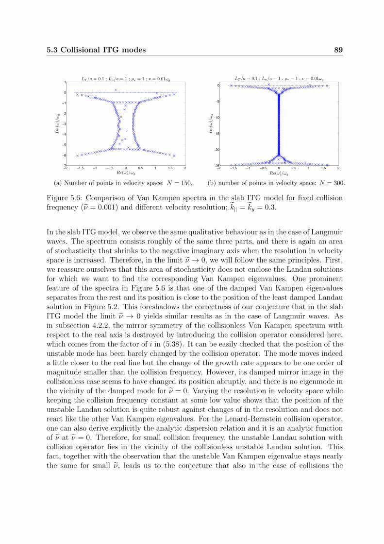
5.3 Collisional ITG modes 89
−2 −1.5 −1 −0.5 0 0.5 1 1.5 2−7
−6
−5
−4
−3
−2
−1
0
1
Re(ω)/ωg
Im(ω
)/ωg
LT /a = 0.1 ; Ln/a = 1 ; ρ∗ = 1 ; ν = 0.01ωg
(a) Number of points in velocity space: N = 150.
−2 −1.5 −1 −0.5 0 0.5 1 1.5 2−25
−20
−15
−10
−5
0
Re(ω)/ωg
Im(ω
)/ωg
LT /a = 0.1 ; Ln/a = 1 ; ρ∗ = 1 ; ν = 0.01ωg
(b) number of points in velocity space: N = 300.
Figure 5.6: Comparison of Van Kampen spectra in the slab ITG model for fixed collisionfrequency (ν = 0.001) and different velocity resolution; k|| = ky = 0.3.
In the slab ITG model, we observe the same qualitative behaviour as in the case of Langmuirwaves. The spectrum consists roughly of the same three parts, and there is again an areaof stochasticity that shrinks to the negative imaginary axis when the resolution in velocityspace is increased. Therefore, in the limit ν → 0, we will follow the same principles. First,we reassure ourselves that this area of stochasticity does not enclose the Landau solutionsfor which we want to find the corresponding Van Kampen eigenvalues. One prominentfeature of the spectra in Figure 5.6 is that one of the damped Van Kampen eigenvaluesseparates from the rest and its position is close to the position of the least damped Landausolution in Figure 5.2. This foreshadows the correctness of our conjecture that in the slabITG model the limit ν → 0 yields similar results as in the case of Langmuir waves. Asin subsection 4.2.2, the mirror symmetry of the collisionless Van Kampen spectrum withrespect to the real axis is destroyed by introducing the collision operator considered here,which comes from the factor of i in (5.38). It can be easily checked that the position of theunstable mode has been barely changed by the collision operator. The mode moves indeeda little closer to the real line but the change of the growth rate appears to be one order ofmagnitude smaller than the collision frequency. However, its damped mirror image in thecollisionless case seems to have changed its position abruptly, and there is no eigenmode inthe vicinity of the damped mode for ν = 0. Varying the resolution in velocity space whilekeeping the collision frequency constant at some low value shows that the position of theunstable Landau solution is quite robust against changes of in the resolution and does notreact like the other Van Kampen eigenvalues. For the Lenard-Bernstein collision operator,one can also derive explicitly the analytic dispersion relation and it is an analytic functionof ν at ν = 0. Therefore, for small collision frequency, the unstable Landau solution withcollision operator lies in the vicinity of the collisionless unstable Landau solution. Thisfact, together with the observation that the unstable Van Kampen eigenvalue stays nearlythe same for small ν, leads us to the conjecture that also in the case of collisions the
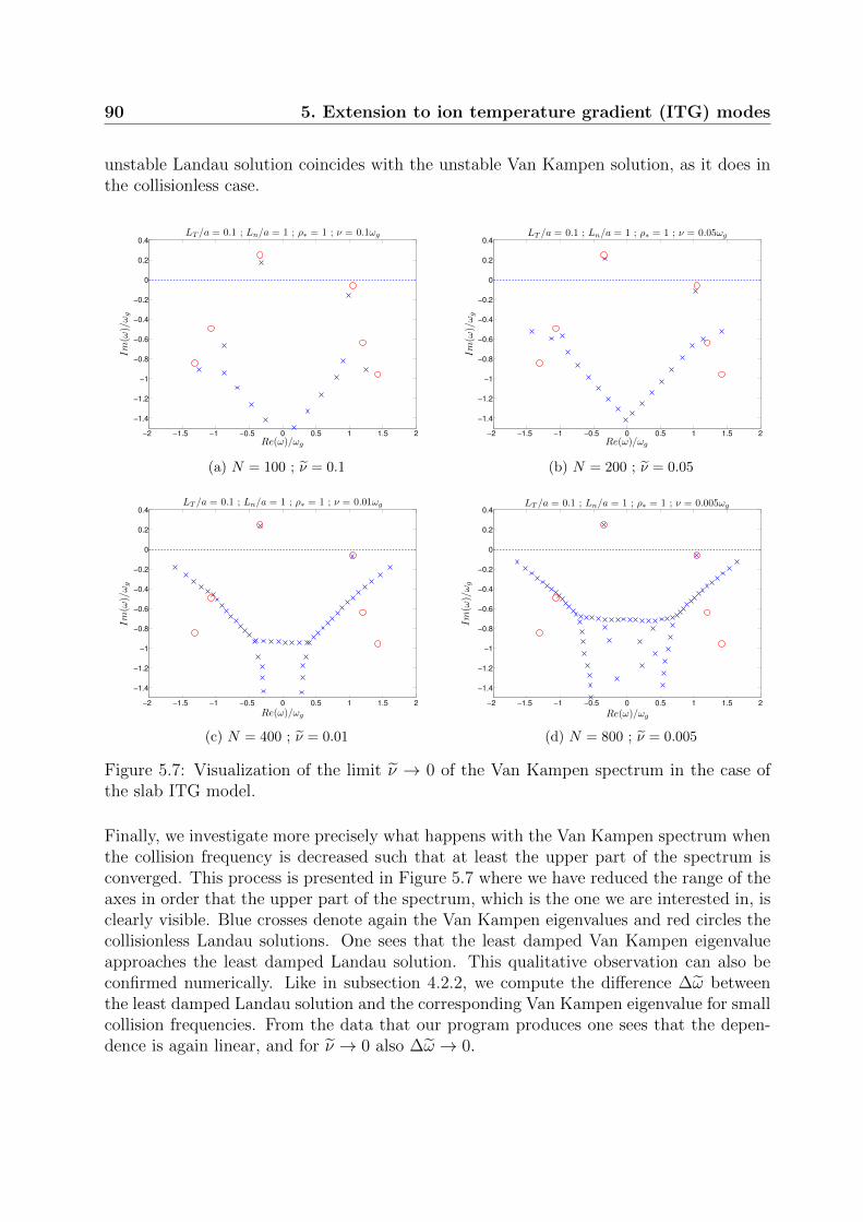
90 5. Extension to ion temperature gradient (ITG) modes
unstable Landau solution coincides with the unstable Van Kampen solution, as it does inthe collisionless case.
−2 −1.5 −1 −0.5 0 0.5 1 1.5 2
−1.4
−1.2
−1
−0.8
−0.6
−0.4
−0.2
0
0.2
0.4
Re(ω)/ωg
Im(ω
)/ωg
LT /a = 0.1 ; Ln/a = 1 ; ρ∗ = 1 ; ν = 0.1ωg
(a) N = 100 ; ν = 0.1
−2 −1.5 −1 −0.5 0 0.5 1 1.5 2
−1.4
−1.2
−1
−0.8
−0.6
−0.4
−0.2
0
0.2
0.4
Re(ω)/ωg
Im(ω
)/ωg
LT /a = 0.1 ; Ln/a = 1 ; ρ∗ = 1 ; ν = 0.05ωg
(b) N = 200 ; ν = 0.05
−2 −1.5 −1 −0.5 0 0.5 1 1.5 2
−1.4
−1.2
−1
−0.8
−0.6
−0.4
−0.2
0
0.2
0.4
Re(ω)/ωg
Im(ω
)/ωg
LT /a = 0.1 ; Ln/a = 1 ; ρ∗ = 1 ; ν = 0.01ωg
(c) N = 400 ; ν = 0.01
−2 −1.5 −1 −0.5 0 0.5 1 1.5 2
−1.4
−1.2
−1
−0.8
−0.6
−0.4
−0.2
0
0.2
0.4
Re(ω)/ωg
Im(ω
)/ωg
LT /a = 0.1 ; Ln/a = 1 ; ρ∗ = 1 ; ν = 0.005ωg
(d) N = 800 ; ν = 0.005
Figure 5.7: Visualization of the limit ν → 0 of the Van Kampen spectrum in the case ofthe slab ITG model.
Finally, we investigate more precisely what happens with the Van Kampen spectrum whenthe collision frequency is decreased such that at least the upper part of the spectrum isconverged. This process is presented in Figure 5.7 where we have reduced the range of theaxes in order that the upper part of the spectrum, which is the one we are interested in, isclearly visible. Blue crosses denote again the Van Kampen eigenvalues and red circles thecollisionless Landau solutions. One sees that the least damped Van Kampen eigenvalueapproaches the least damped Landau solution. This qualitative observation can also beconfirmed numerically. Like in subsection 4.2.2, we compute the difference ∆ω betweenthe least damped Landau solution and the corresponding Van Kampen eigenvalue for smallcollision frequencies. From the data that our program produces one sees that the depen-dence is again linear, and for ν → 0 also ∆ω → 0.

5.3 Collisional ITG modes 91
Having validated numerically this conjecture, the next step is to investigate the modestructures of typical Van Kampen eigenmodes. This is done in the same way as in subsec-tion 4.2.2, namely by numerically computing the second derivative of the correspondingmode with respect to velocity, and taking the maximum of its absolute value which wecall again dmax. We focus our attention on three modes: the unstable mode, the one thatapproaches the least damped Landau solution and the mode in the upper left corner of theVan Kampen spectrum. For the unstable mode, we observed that dmax indeed grows whenthe collision frequency is decreased but the changes were very small. For a decrease of ν bya factor of 10, dmax increased by a factor of nearly 2. From this follows that the productν · dmax will tend to zero in the limit ν → 0, i.e., the unstable Van Kampen mode has atrivial limit which is what we expected, since the unstable Landau solution is a continuousfunction of ν. Next, we perform the same numerical computation for the Van Kampenmode that approaches the least damped Landau solution. Here dmax scales approximatelylinearly with the inverse collision frequency which means that the product ν ·dmax does nottend to zero in the limit ν → 0, confirming our observations of the Van Kampen spectrum.For the Van Kampen mode in the upper left corner of the spectrum noticeable changesof dmax were observed when collision frequency decreased. Therefore, the functional de-pendence of the second derivative was parametrized as dmax = y1 · (1/ν)y2 + y3, since thisparametrization was successful in the case of Langmuir waves. The best such fit to ourdata yielded for the parameter y2 a value of approximatively 0.83. This means that theproduct ν · dmax scales like ν0.17, i.e., this mode also has a trivial limit when the collisionfrequency goes to zero.As one sees in this chapter, many features of the Langmuir waves carry over to the slabITG model. From a physical point of view, this can be considered as an unexpected result,since in the second case, one deals with strongly magnetized plasmas where also gradientsin density and temperature are present.

92 5. Extension to ion temperature gradient (ITG) modes
Chapter 6
Summary and conclusions
In chapter 1, we motivated this work by highlighting the importance of kinetic effects likeLandau damping for the physical understanding turbulent plasmas. In chapter 3, we formu-lated the problem of Langmuir waves in a mathematically rigorous way. To our knowledge,such an in-depth treatment cannot be found anywhere in the literature. Although this didnot change the fundamental physics of Landau damping, of course, it helped to gain usefulinsights into the structure and origin of the Van Kampen spectrum. At the end of thatchapter, we also arrived at the conclusion that some standard references about Landaudamping such as [13] do not give the correct picture of the conditions under which the VanKampen spectrum arises. The consequences of this finding should be investigated further.
In chapter 4, we treated the problem of Langmuir waves numerically. One of the mostinteresting aspects in the collisionless case was to explore which of the Van Kampen eigen-modes are most important for the large-time evolution of the system and the occurrenceof an exponentially damped electric field. It was expected that these are the modes thatlie above the least damped Landau solutions in the complex frequency plane where an ac-cumulation of eigenvalues was observed, since they also have the largest coefficients whena typical initial condition is decomposed into the basis of Van Kampen modes. However,it turned out that these modes alone are not sufficient for reproducing Landau dampingand that one should also consider the modes that lie in the middle part of the spectrum,although their coefficients are rather small.Another important part of this work was to show numerically that the Van Kampen spec-trum changes abruptly when collisions are introduced into the system via the Lenard-Bernstein collision operator as stated in [18], [15], and [16]. Since this conjecture has beenproved analytically, our goal was rather to investigate if a numerical discretization in veloc-ity space, that is widely used in computer simulations in plasma physics, reproduces thiseffect. From our analysis, this appears to be the case. We also went one step further andinvestigated which part of the Lenard-Bernstein collision operator is responsible for thisbehaviour. It became clear that the reason was the term in the operator which involves asecond derivative of the perturbation with respect to velocity. One usually refers to thisas diffusion in velocity space, and it is also present into the full Focker-Planck collision

94 6. Summary and conclusions
operator. Therefore, if one considers simplified models for collision operators, one shouldalso include this feature in order to reproduce physically correct results.In chapter 5, we studied a slab ITG model. It turned out that it is mathematically verysimilar to the model of electrostatic Langmuir waves, and we observed that many of itsessential features carry over to the slab ITG case. This applies also to the effect of collisions.
The work presented here can be extended to physically more realistic situations. Furtherinvestigations of Landau damping can improve our understanding for the influence of ki-netic effects on the behaviour of turbulent fusion plasmas. One of its important featuresthat has to be clarified is the saturation of turbulent flows and the energy transfer be-tween unstable and damped modes with similar wave numbers, since this appears to bethe greatest difference between plasma turbulence and conventional fluid turbulence. Thelinear theory used in this work can help us gain important physical insights which can leadto improved models of nonlinear effects, allowing for more efficient computer simulationsof fusion plasmas.

Appendix A
Relations involving the plasmadispersion function Z
The exact definition of the plasma dispersion function Z given in [1] is
Z(ξ) =1√π
+∞∫
−∞
e−x2
x− ξ dx, (A.1)
where ξ ∈ C and the above expression applies for Imξ > 0. For Imξ ≤ 0, one should takethe analytical continuation of (A.1) which, as we saw, is given by doing the integrationfrom −∞ to +∞ along the Landau contour. Here, for convenience, we are going to keepthe boundaries of the integrals as in (A.1) but one should keep in mind what the exactintegration prescription is. The first relation in (5.24) is clear, so we focus on the secondand third one:
+∞∫
−∞
xe−bx2
x− a dx =
+∞∫
−∞
(x− a+ a)e−bx2
x− a dx =
+∞∫
−∞
e−bx2
dx
︸ ︷︷ ︸=√
πb
+a
+∞∫
−∞
e−bx2
x− adx
︸ ︷︷ ︸=√πZ(a
√b)
=
=
√π
b+ a√πZ(a
√b);
(A.2)
+∞∫
−∞
x2e−bx2
x− a dx =
+∞∫
−∞
(x2 − a2 + a2)e−bx2
x− a dx =
+∞∫
−∞
xe−bx2
dx
︸ ︷︷ ︸=0
+a
+∞∫
−∞
e−bx2
dx
︸ ︷︷ ︸=√
πb
+ (A.3)

96 A. Relations involving the plasma dispersion function Z
+a2
+∞∫
−∞
e−bx2
x− adx
︸ ︷︷ ︸=√πZ(a
√b)
= a
√π
b+ a2√πZ(a
√b).
In previous chapters of this work, we occasionally used a decomposition of Z into its realand imaginary part for arguments with a positive imaginary part. In that case, one canrepresent the plasma dispersion function via (A.1), and this integral is well defined sincethere are no poles lying on the integration path. If ξ := x + iy, where x,y ∈ R, one canwrite
Z(ξ) = Z(x, y) =1√π
+∞∫
−∞
e−t2(t− (x− iy))
|t− x− iy|2 dt =1√π
+∞∫
−∞
(t− x)e−t2
(t− x)2 + y2dt
︸ ︷︷ ︸=ReZ(x,y) for y>0
+
+ i y1√π
+∞∫
−∞
e−t2
(t− x)2 + y2dt
︸ ︷︷ ︸=ImZ(x,y) for y>0
. (A.4)
In section 2.2, we also used that the partial derivative of ImZ(x, y) with respect to x canbe commuted with the integration with respect to t. In order to prove this, we first notethat the derivative of the integrand is
∂
∂x
(e−t
2
(t− x)2 + y2
)=
2(t− x)e−t2
((t− x)2 + y2)2
which exist for all x and t, since y ∈ R+. Now, we only have to verify that the integral ofthis expression over t is finite, which can be done as follows:
+∞∫
−∞
2(t− x)e−t2
((t− x)2 + y2)2dt = 2
+∞∫
−∞
te−t2
((t− x)2 + y2)2dt− 2x
+∞∫
−∞
e−t2
((t− x)2 + y2)2dt
︸ ︷︷ ︸≤ 1y4
∫+∞−∞ e−t2dt=
√π
y4<+∞
(A.5)
and the first integral can be estimated with

97
∣∣∣∣∣∣
+∞∫
−∞
te−t2
((t− x)2 + y2)2dt
∣∣∣∣∣∣≤
+∞∫
−∞
|t|e−t2
((t− x)2 + y2)2dt ≤ 1
y4
+∞∫
−∞
|t|e−t2dt =
=2
y4
+∞∫
0
te−t2
dt =1
y4< +∞, (A.6)
i.e., the left-hand side of (A.5) is a sum of two finite terms and is therefore also finite.
98 A. Relations involving the plasma dispersion function Z

Appendix B
Employed MATLAB codes
In this part of the Appendix, we present the codes that we used to produce the resultsdescribed in this thesis.
function[nooutput,f] = landau(n,kapa)
v = [0:.001:0.02];
[Re_w,Im_w] = meshgrid(-n:.001:n, -n:.001:0);
f1 = 1 + kapa^2 + 1i*(1/kapa)*sqrt(pi/2).*(Re_w +
1i*Im_w).*faddeeva((Re_w+1i*Im_w)/(sqrt(2)*kapa));
f = sqrt(real(f1).^2 + imag(f1).^2);
plot([n -n], [0 0], ’--’);
hold on
contour(Re_w, Im_w, f, v);
xlabel(’$Re(\omega)/\omega_{pe}$’, ’Interpreter’, ’latex’, ’FontSize’, 30,
’FontName’,’Courier’);
ylabel(’$Im(\omega)/\omega_{pe}$’, ’Interpreter’, ’latex’, ’FontSize’, 30,
’FontName’,’Courier’);
title([’contour plot of the Landau solutions for k = ’, num2str(kapa),
’\lambda_{D}’]);
————————————————————————————————
% calculates eigenvalues, eigenvectors and spectral density of the matrix M
function[nooutput,E] = eigenvalue(v_max,N,kapa)
v = linspace(-v_max,v_max,N+1); % row of the vector v
delta_v = v(2) - v(1);
G = -v.*exp(-(v.^2)/2)/sqrt(2*pi);
a = 1:N+1;

100 B. Employed MATLAB codes
b = ones(1,N+1);
M1 = -kapa*v_max*((N+2)/N)*eye(N+1);
M2 = kapa*delta_v*diag(a);
M3 = -(delta_v*G.’*b)/kapa;
M = M1 + M2 + M3;
[V,E] = eig(M);
E = diag(E);
[new_E,inds] = sort(E);
V = V(:,inds);
V = V*diag(1./sum(V))/delta_v;
plot(real(E), imag(E), ’x’, ’MarkerSize’, 15);
hold on
plot(real(new_E(1:end-1)), delta_v./diff(real(new_E)));
xlabel(’$Re(\omega)/\omega_{pe}$’, ’Interpreter’, ’latex’,
’FontSize’, 34, ’FontName’,’Courier’);
ylabel(’$Im(\omega)/\omega_{pe}$’, ’Interpreter’, ’latex’,
’FontSize’, 34, ’FontName’,’Courier’);
ylabel(’spectral density’, ’FontSize’, 34, ’FontName’, ’Courier’)
title([’$v_{max} = $ ’ , num2str(v_max), ’$v_{th}$ ’, ’ $ ; \Delta v = $ ’,
num2str(delta_v), ’$v_{th}$ ’, ’ $ ; k\lambda_{D} = $ ’, num2str(kapa)],
’Interpreter’, ’latex’, ’FontSize’, 34, ’FontName’, ’Courier’);
set(gca, ’FontSize’, 24)
————————————————————————————————
% calculates the perturbation of the distribution function as an
% initial value problem
function[kapa,D,V,W,F] = initial_value(v_max,N,t_max,N_time)
kapa = 0.5;
t = linspace(0,t_max,N_time);
v = linspace(-v_max,v_max,N+1);
delta_v = v(2) - v(1);
a = 1:N+1;
G = -v.*exp(-(v.^2)/2)/sqrt(2*pi);
101
b = ones(1,N+1);
M1 = -kapa*v_max*((N+2)/N)*eye(N+1);
M2 = kapa*delta_v*diag(a);
M3 = -(delta_v*G.’*b)/kapa;
M = M1 + M2 + M3;
[V,D] = eig(M);
D = diag(D);
[D,inds] = sort(D);
V = V(:,inds);
V = V*diag(1./sum(V))/delta_v;
[W,E_l] = eig(M.’);
E_l = diag(E_l);
[~,inds] = sort(E_l);
W = W(:,inds);
W = W*diag(1./sum(W))/delta_v;
clear M;
F_0 = exp(-(v).^2/2);
COEF = zeros(1,N+1);
for j = 1:N+1
COEF(j) = (W(:,j)’*F_0’)/(W(:,j)’*V(:,j));
end
B = exp(multiprod(-1i*diag(D),permute(t,[1 3 2])))-repmat(ones(N+1,’single’)
-eye(N+1,’single’),[1 1 N_time]);
C = multiprod(multiprod(V,B),inv(V));
clear B;
F = squeeze(multiprod(C,F_0’));
clear C;
————————————————————————————————
% Van Kampen spectrum in the case of a ’bump-on-tail’ background distribution
% in velocity space
102 B. Employed MATLAB codes
function[nooutput,f] = bump(v_max,N,C_a,v_b,tau)
v = linspace(-v_max,v_max,N+1);
delta_v = v(2) - v(1);
kapa = 0.5;
G = - (C_a/sqrt(2*pi))*v.*exp(-v.^2/2) -
((1-C_a)*tau^(3/2)/sqrt(2*pi))*(v-v_b).*exp(-tau*((v-v_b).^2)/2);
a = 1:N+1;
b = ones(1,N+1);
M1 = -kapa*v_max*((N+2)/N)*eye(N+1);
M2 = kapa*delta_v*diag(a);
M3 = -(delta_v*G.’*b)/kapa;
M = M1 + M2 + M3;
[~,E] = eig(M);
E = diag(E);
[new_E,inds] = sort(real(E));
V = V(:, inds);
V = V*diag(1./sum(V))/delta_v;
plot(real(E), imag(E), ’x’, ’MarkerSize’, 15);
hold on
landau_bump(kapa,C_a,v_b,tau);
xlabel(’$Re(\omega)/\omega_{pe}$’, ’Interpreter’, ’latex’, ’FontSize’,
34, ’FontName’, ’Courier’);
ylabel(’$Im(\omega)/\omega_{pe}$’, ’Interpreter’, ’latex’, ’FontSize’,
34, ’FontName’, ’Courier’);
title([’$v_{max} = $ ’, num2str(v_max), ’$v_{th}$ ’, ’ $; \Delta v = $ ’,
num2str(delta_v), ’$v_{th}$’, ’ $; C_{a} = $ ’, num2str(C_a), ’ $;
v_{b} = $ ’, num2str(v_b), ’$v_{th}$’, ’ $; \tau = $ ’, num2str(tau)],
’Interpreter’, ’latex’, ’FontSize’, 34, ’FontName’, ’Courier’);
set(gca, ’FontSize’, 24)
————————————————————————————————
% Landau approach for the ‘bump-on-tail’ instability
function[nooutput,f] = landau_bump(kapa,C_a,v_b,tau)

103
v = [0:.004:0.02];
[Re_w,Im_w] = meshgrid(-4:10^(-4):4, -1:10^(-4):0.5);
f1 = kapa^2 + tau + C_a*(1-tau) + 1i*sqrt(pi)*C_a*((Re_w +
1i*Im_w)/(sqrt(2)*kapa)).*faddeeva((Re_w+1i*Im_w)/(sqrt(2)*kapa)) +...
+ 1i*sqrt(pi)*(1-C_a)*tau*sqrt(tau/2)*(((Re_w +
1i*Im_w)/kapa)-v_b).*faddeeva(sqrt(tau/2)*(((Re_w + 1i*Im_w)/kapa)-v_b));
f = sqrt(real(f1).^2 + imag(f1).^2);
contour(Re_w, Im_w, f, v);
xlabel(’$Re(\omega)/\omega_{pe}$’, ’Interpreter’, ’latex’, ’FontSize’, 34,
’FontName’, ’Courier’);
xlabel(’$Im(\omega)/\omega_{pe}$’, ’Interpreter’, ’latex’, ’FontSize’, 34,
’FontName’, ’Courier’);
title([’$v_{max} = $ ’, num2str(v_max), ’$v_{th}$ ’, ’ $; \Delta v = $ ’,
num2str(delta_v), ’$v_{th}$’, ’ $; C_{a} = $ ’, num2str(C_a),
’ $; v_{b} = $ ’, num2str(v_b), ’$v_{th}$’, ’ $; \tau = $ ’, num2str(tau)],
’Interpreter’, ’latex’, ’FontSize’, 34, ’FontName’, ’Courier’);
set(gca, ’FontSize’, 24)
————————————————————————————————
% calculates eigenvalues and spectral density of the matrix M for the slab
% ITG model
function[nooutput,E] = drift_eigenvalue(v_max,N,L_T,L_n)
v = linspace(-v_max,v_max,N+1);
delta_v = v(2) - v(1);
a = 1:N+1;
b = ones(1,N+1);
tau = 1;
k_y = 0.3;
k_par = 0.03;
ro = 0.01;
G = tau*exp(-(v.^2)/2).*( k_y/(2*L_T) - (k_y/(2*L_T))*v.^2 - k_y/L_n -
k_par*v )/sqrt(2*pi);
M1 = k_par*v_max*((N+2)/N)*eye(N+1);
M2 = -k_par*delta_v*diag(a);
M3 = (delta_v*G.’*b);

104 B. Employed MATLAB codes
M = -(M1 + M2 + M3);
[V,E] = eig(M);
E = ro*diag(E);
[new_E,inds] = sort(real(E));
V = V(:,inds);
V = V*diag(1./sum(V))/delta_v;
clear M;
plot(real(E), imag(E), ’x’, ’MarkerSize’, 24);
hold on
plot(new_E(1:end-1), delta_v./diff(new_E));
hold on
drift_landau(ro,L_T,L_n);
xlabel(’$Re(\omega)/\omega_{g}$’, ’Interpreter’, ’latex’, ’FontSize’, 40,
’FontName’, ’Courier’);
ylabel(’$Im(\omega)/\omega_{g}$’, ’Interpreter’, ’latex’, ’FontSize’, 40,
’FontName’, ’Courier’);
title([’$v_{||,max}/v_{th} = $ ’, num2str(v_max), ’ $ ; \Delta v_{||}/v_{th} = $ ’,
num2str(delta_v), ’ $ ; \widetilde{L}_{T} = $ ’,num2str(L_T), ’ $ ;
\widetilde{L}_{n} = $’,num2str(L_n)], ’Interpreter’, ’latex’, ’FontSize’,
40, ’FontName’, ’Courier’);
set(gca, ’FontSize’, 30)
————————————————————————————————
% This program computes the Landau solutions arising from the linerized
% drift-kinetic equation for the distribution function gyrocenters where
% only a ExB drift has benn considered
function [nooutput,f] = drift_landau(ro,L_T,L_n)
tau = 1;
k_y = 0.3;
k_par = 0.3;
v = [0:0.1:1]*10^(-4);
[Re_w,Im_w] = meshgrid(1.418:10^(-5):1.428, -0.962:10^(-5):-0.952);
f1 = 1 + tau + 0.5*tau*(k_y/k_par)*(1/L_T)*(Re_w + 1i*Im_w)/(k_par*ro) +
1i*tau*sqrt(pi).*faddeeva((Re_w + 1i*Im_w)/(sqrt(2)*k_par*ro)).*( (Re_w +
1i*Im_w)/(sqrt(2)*k_par*ro) - (k_y/k_par)*( 1/(2*L_T) - 1/L_n )/sqrt(2) +
105
sqrt(1/2)*(k_y/k_par)*((Re_w + 1i*Im_w)/(sqrt(2)*k_par*ro)).^2/L_T );
f = real(f1).^2 + imag(f1).^2;
contour(Re_w, Im_w, f, v);
xlabel(’$Re(\omega)/\omega_{g}$’, ’Interpreter’, ’latex’, ’FontSize’, 30);
ylabel(’$Im(\omega)/\omega_{g}$’, ’Interpreter’, ’latex’, ’FontSize’, 30);
title([’v_{max}/v_{th} = ’, num2str(v_max), ’ ; \Deltav/v_{th} = ’,
num2str(delta_v) ’ ; k_{||}*a = ’, num2str(k_par), ’ ; k_{y}*r_{L} = ’,
num2str(k_y), ’ ; L_{T}/a = ’,num2str(L_T), ’; L_{n}/a = ’,num2str(L_n),
’ ; \rho_{*} = ’, num2str(ro)], ’FontSize’, 24, ’FontName’, ’Courier’);
set(gca, ’FontSize’, 18)
———————————————————————————————–
% calculates eigenvalues and spectral density of the matrix M for Langmuir
% waves where collisions are involved via the Lenard-Bernstein collision
% operator
function[nooutput,E] = Lenard_Bernstein(v_max,N,nu)
v = linspace(-v_max,v_max,N+1);
delta_v = v(2) - v(1);
G = -v.*exp(-(v.^2)/2)/sqrt(2*pi);
kapa = 0.5;
a = 1:N+1;
b = ones(1,N+1);
M = -kapa*v_max*((N+2)/N)*eye(N+1) + kapa*delta_v*diag(a) - (delta_v*G.’*b)/kapa
+ 1i*nu*(eye(N+1) + (-((N+2)/4)*eye(N+1) + (1/2)*diag(a))*(diag(b(1:N),1) -
diag(b(1:N),-1))+(diag(b(1:N),1)-2*eye(N+1)+diag(b(1:N),-1))*(1/(delta_v^2)));
[V,E] = eig(M);
E = diag(E);
[~,inds] = sort(abs(E - 1.41566179 + 1i*0.15335939));
V = V(:,inds);
V = V*diag(1./sum(V))/delta_v;
plot(real(E), imag(E), ’x’, ’MarkerSize’, 24);
xlabel(’$Re(\omega/\omega_{pe})$’, ’Interpreter’, ’latex’, ’FontSize’, 40,
’FontName’, ’Courier’);

106 B. Employed MATLAB codes
ylabel(’$Im(\omega/\omega_{pe})$’, ’Interpreter’, ’latex’, ’FontSize’, 40,
’FontName’, ’Courier’);
title([’$v_{max} = $ ’, num2str(v_max), ’$v_{th} ; \nu = $ ’, num2str(nu),
’$\omega_{pe}$’ ,’ $ ; N = $ ’, num2str(N)], ’Interpreter’, ’latex’,
’FontSize’, 40, ’FontName’, ’Courier’);
set(gca, ’FontSize’, 40)
————————————————————————————————
% calculates eigenvalues and spectral density of the matrix M for the slab
% ITG model where collisions are involved via the Lenard-Bernstein collision
% operator
function[nooutput,E] = drift_eigenvalue_Lenard(v_max,N,L_T,L_n,nu)
v = linspace(-v_max,v_max,N+1);
delta_v = v(2) - v(1);
a = 1:N+1;
b = ones(1,N+1);
tau = 1;
k_y = 0.3;
k_par = 0.3;
ro = 1;
G = tau*exp(-(v.^2)/2).*( k_y/(2*L_T) - (k_y/(2*L_T))*v.^2 - k_y/L_n -
k_par*v )/sqrt(2*pi);
M1 = k_par*v_max*((N+2)/N)*eye(N+1);
M2 = -k_par*delta_v*diag(a);
M3 = (delta_v*G.’*b);
M = -(M1 + M2 + M3) + 1i*(1/ro)*nu*( eye(N+1) + (-(N/4)*eye(N+1) -
(1/2)*eye(N+1) + (1/2)*diag(a))*(diag(b(1:N),1) - diag(b(1:N),-1)) +
(diag(b(1:N),1) - 2*eye(N+1) + diag(b(1:N),-1))*(1/(delta_v^2)) );
[V,E] = eig(M);
E = ro*diag(E);
[~,inds] = sort(imag(E), ’descend’);
V = V(:,inds);
V = V*diag(1./sum(V))/delta_v;
107
plot(real(E), imag(E), ’x’, ’Markersize’, 24);
hold on
drift_landau(ro,L_T,L_n);
xlabel(’$Re(\omega)/\omega_{g}$’, ’Interpreter’, ’latex’, ’FontSize’, 40,
’FontName’, ’Courier’);
ylabel(’$Im(\omega)/\omega_{g}$’, ’Interpreter’, ’latex’, ’FontSize’, 40,
’FontName’, ’Courier’);
title([’$L_{T}/a = $ ’,num2str(L_T), ’ ; $L_{n}/a = $ ’,num2str(L_n),
’ ; $\rho_{\ast}= $ ’,num2str(ro), ’ ; $\nu = $ ’, num2str(nu),
’$\omega_{g}$’], ’Interpreter’, ’latex’, ’FontSize’, 40, ’FontName’,
’Courier’);
set(gca, ’FontSize’, 30)
————————————————————————————————
% reduced Lenard-Bernstein collision operator (only the first and the
% third part are present)
function[nooutput,E] = Lenard_Bernstein_2(v_max,N,nu)
v = linspace(-v_max,v_max,N+1);
delta_v = v(2) - v(1);
G = -v.*exp(-(v.^2)/2)/sqrt(2*pi);
kapa = 0.5;
a = 1:N+1;
b = ones(1,N+1);
M1 = -kapa*v_max*((N+2)/N)*eye(N+1);
M2 = kapa*delta_v*diag(a);
M3 = -(delta_v*G.’*b)/kapa;
M = M1 + M2 + M3 + 1i*nu*( eye(N+1) + (diag(b(1:N),1) - 2*eye(N+1) +
diag(b(1:N),-1))*(1/(delta_v^2)) );
[V,E] = eig(M);
E = diag(E);
[E_new,inds] = sort(E);
V = V(:,inds);
plot(real(E), imag(E), ’x’, ’MarkerSize’, 24);
hold on

108 B. Employed MATLAB codes
xlabel(’$Re(\omega/\omega_{pe})$’, ’Interpreter’, ’latex’, ’FontSize’,
40, ’FontName’, ’Courier’);
ylabel(’$Im(\omega/\omega_{pe})$’, ’Interpreter’, ’latex’, ’FontSize’,
40, ’FontName’, ’Courier’);
title([’$v_{max} = $ ’, num2str(v_max), ’$v_{th} $ ’, ’ $ ; N = $ ’,
num2str(N)], ’Interpreter’, ’latex’, ’FontSize’, 40, ’FontName’,
’Courier’);
set(gca, ’FontSize’, 40)
————————————————————————————————
% implements the Newton-Rapson method for finding zeros of a given function
function [nooutput,w] = my_newton(start,max,tol,kapa)
for j = 1:max
w = start;
w = w - sqrt(2)*kapa*(1 + kapa^2 + (w/(sqrt(2)*kapa))*1i*sqrt(pi)*
*faddeeva(w/(sqrt(2)*kapa)))/(1i*sqrt(pi)*faddeeva(w/(sqrt(2)*kapa))*
*(1 - 2*(w/(sqrt(2)*kapa))^2) - 2*w/(sqrt(2)*kapa));
if (abs((w - start)/w) < tol)
fprintf(1,’Newton converged\n\n answer is: omega = %11.8f %+11.8fi\n\n’,
real(w), imag(w));
break
end
start = w;
end
———————————————————————————————–
% implements the decomposition in a basis involving Hermite polynomials
% according to Ng and Bhattacharjee
function[nooutput,M] = test_Ng(n,nu)
a = 1:n;
b = 1:n+1;
kapa = 0.5;
M1 = diag(sqrt(a),-1) + diag(sqrt(a),1);

109
M1(2,1) = M1(2,1) + 1/kapa^2;
M = kapa*M1 - 1i*nu*diag(b-1);
[~,E] = eig(M);
E = diag(E);
plot(real(E), imag(E), ’x’, ’MarkerSize’, 24);
xlabel(’$Re(\omega)/\omega_{pe}$’, ’Interpreter’, ’latex’, ’FontSize’, 40,
’FontName’, ’Courier’);
ylabel(’$Im(\omega)/\omega_{pe}$’, ’Interpreter’, ’latex’, ’FontSize’, 40,
’FontName’, ’Courier’);
title([’$n = $ ’ , num2str(n), ’ $ ; \nu = $ ’, num2str(nu), ’$\omega_{pe}$’,
’ $ ; k\lambda_{D} = $ ’ , num2str(kapa)], ’Interpreter’, ’latex’,
’FontSize’, 40, ’FontName’, ’Courier’);
set(gca, ’FontSize’, 30)
The program faddeeva.m implements the plasma dispersion function and has been down-loaded from www.mathworks.com.

110 B. Employed MATLAB codes

Bibliography
[1] The Plasma Dispersion Function, Burton D. Fried and Samuel D. Conte (AcademicPress, London 1961)
[2] Theoretische Plasmaphysik, K. H. Spatschek (Teubner, Stuttgart 1990)
[3] Plasmaphysik, Robert J. Goldstone and Paul H. Rutherford (Vieweg, 1998)
[4] Introduction to Plasma Theory, Dwight R. Nicholson (John Wiley, 1983)
[5] Plasma Confinement, R. D. Hazeltine and J. D. Meiss (Dover Publications, 2003)
[6] Methods of Modern Mathematical Physics, IV: Analysis of Operators, M. Reed andB. Simon (Academic Press, 1978)
[7] Lineare Operatoren in Hilbertraumen, Teil I Grundlagen, J. Weidmann (Teubner,2000)
[8] Theoretical Methods in Plasma Physics, N. G. Van Kampen and B. U. Felderhof(North-Holland, Amsterdam 1967)
[9] Fundamentals of Plasma Physics and Controlled Fusion, Kenro Miyamoto (IwanamiBook Service Center, 1997)
[10] Modern Plasma Physics, Volume 1, P. H. Diamond, S.-I. Itoh and K. Itoh (CambridgeUniversity Press, 2010)
[11] L. Landau, J. Phys. USSR 10, 25 (1946)
[12] N. G. Van Kampen, Physica 21, 949 (1955)
[13] K. M. Case, Ann. Phys. (N. Y.) 7, 349 (1959)
[14] K. M. Case, Phys. Fluids 8, 96 (1965)
[15] C. S. Ng, A. Bhattacharjee, and F. Skiff, Phys. Rev. Lett. 83, 1974, (1999)
[16] C. S. Ng, A. Bhattacharjee, and F. Skiff, Phys. Rev. Lett. 92, 065002 (2004)
[17] P. L. Bhatnagar, E. P. Gross, and M. Krook, Phys. Rev. 94, 511 (1954)

112 BIBLIOGRAPHY
[18] A. Lenard and I. B. Bernstein, Phys. Rev. 112, 1456 (1958)
[19] T.-H. Watanabe and H. Sugama, Phys. Plasmas 11, 1476 (2004)
[20] S. C. Cowley, R. M. Kulsrud and R. Sudan, Phys. Fluids B 3, 2767 (1991)
[21] F. Jenko, W. Dorland, M. Kotschenreuther, B. N. Rogers, Phys. Plasmas 7, 1904(2000)
[22] G. W. Hammett, W. Dorland and F. W. Perkins, Phys. Rev. Lett. 106, 115003 (2011)
[23] C. H. Su and C. Oberman, Phys. Rev. Lett. 20, 427 (1968)
[24] D. R. Hatch, P. W. Terry, F. Jenko, F. Merz, M. J. Pueschel, W. M. Nevins and E.Wang, Phys. Plasmas 18, 055706 (2011)
[25] D. R. Hatch, P. W. Terry, F. Jenko, F. Merz and W. M. Nevins, Phys. Rev. Lett. 106,115003 (2011)
[26] R. W. Short and A. Simon, Phys. Plasmas 9, 3245 (2002)
[27] private correspondence with D. Hatch
[28] private correspondence with F. Jenko