Lambda Calculus CLC

Computational Lambda Calculus

.

.. ..

.

.

Computational Lambda Calculus

Masato Takeichi

National Institution for Academic Degrees and University Evaluation

May 9, 2011

1 / 38

Computational Lambda CalculusLambda Calculus

References

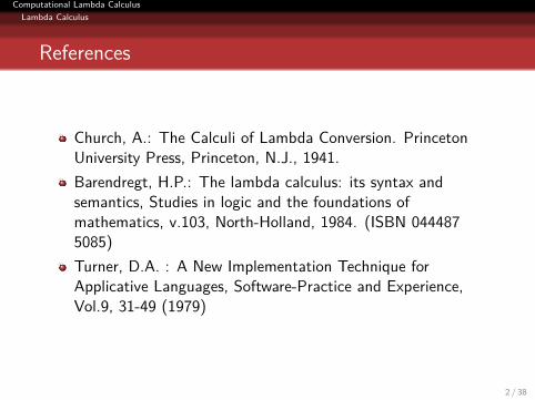
Church, A.: The Calculi of Lambda Conversion. PrincetonUniversity Press, Princeton, N.J., 1941.Barendregt, H.P.: The lambda calculus: its syntax andsemantics, Studies in logic and the foundations ofmathematics, v.103, North-Holland, 1984. (ISBN 0444875085)Turner, D.A. : A New Implementation Technique forApplicative Languages, Software-Practice and Experience,Vol.9, 31-49 (1979)

2 / 38


Lambda Calculus

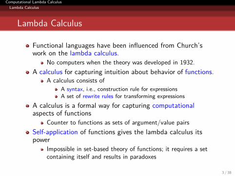
Functional languages have been influenced from Church’swork on the lambda calculus.

No computers when the theory was developed in 1932.A calculus for capturing intuition about behavior of functions.

A calculus consists ofA syntax, i.e., construction rule for expressionsA set of rewrite rules for transforming expressions

A calculus is a formal way for capturing computationalaspects of functions

Counter to functions as sets of argument/value pairsSelf-application of functions gives the lambda calculus itspower

Impossible in set-based theory of functions; it requires a setcontaining itself and results in paradoxes

3 / 38


Lambda Calculus

Lambda Calculus

.Definition (lambda expression)..

.. ..

.

.

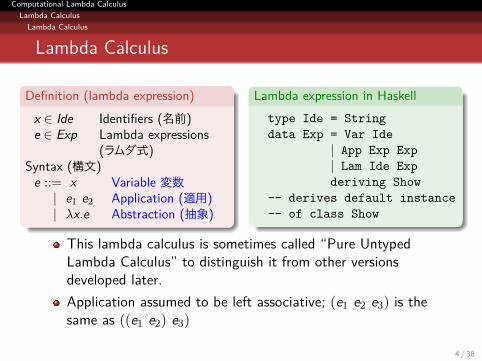
x ∈ Ide Identifiers (名前)e ∈ Exp Lambda expressions

(ラムダ式)Syntax (構文)

e ::= x Variable 変数| e1 e2 Application (適用)| λx.e Abstraction (抽象)

.Lambda expression in Haskell..

.. ..

.

.

type Ide = Stringdata Exp = Var Ide

| App Exp Exp| Lam Ide Expderiving Show

-- derives default instance-- of class Show

This lambda calculus is sometimes called “Pure UntypedLambda Calculus” to distinguish it from other versionsdeveloped later.Application assumed to be left associative; (e1 e2 e3) is thesame as ((e1 e2) e3)

4 / 38


Lambda Calculus

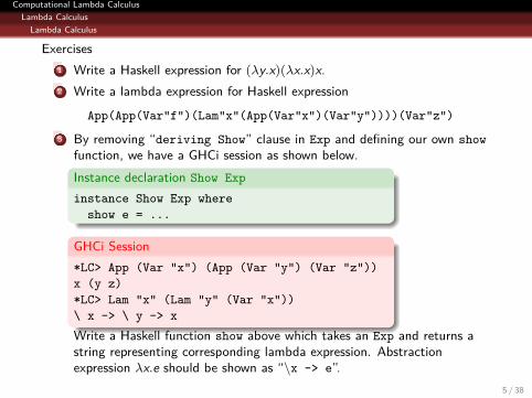
Exercises...1 Write a Haskell expression for (λy.x)(λx.x)x....2 Write a lambda expression for Haskell expression

App(App(Var"f")(Lam"x"(App(Var"x")(Var"y"))))(Var"z")...3 By removing “deriving Show” clause in Exp and defining our own show

function, we have a GHCi session as shown below..Instance declaration Show Exp..

.

. ..

.

.

instance Show Exp whereshow e = ...

.GHCi Session..

.

. ..

.

.

*LC> App (Var "x") (App (Var "y") (Var "z"))x (y z)*LC> Lam "x" (Lam "y" (Var "x"))\ x -> \ y -> xWrite a Haskell function show above which takes an Exp and returns astring representing corresponding lambda expression. Abstractionexpression λx.e should be shown as “\x -> e”.

5 / 38


Rewrite Rules

Free Variables

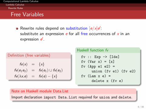
Rewrite rules depend on substitution [e/x]e′:substitute an expression e for all free occurrences of x in anexpression e′.

.Definition (free variables)..

.. ..

.

.fv(x) = {x}

fv(e1e2) = fv(e1) ∪ fv(e2)fv(λx.e) = fv(e)− {x}

.Haskell function fv..

.. ..

.

.

fv :: Exp -> [Ide]fv (Var x) = [x]fv (App e1 e2) =

union (fv e1) (fv e2)fv (Lam x e) =

delete x (fv e)

.Note on Haskell module Data.List..

.. ..

.

.Import declaration import Data.List required for union and delete.

6 / 38


Rewrite Rules

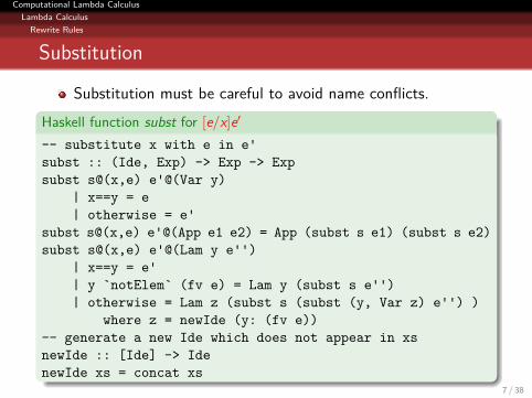
Substitution

Substitution must be careful to avoid name conflicts..Haskell function subst for [e/x]e′..

.. ..

.

.

-- substitute x with e in e'subst :: (Ide, Exp) -> Exp -> Expsubst s@(x,e) e'@(Var y)

| x==y = e| otherwise = e'

subst s@(x,e) e'@(App e1 e2) = App (subst s e1) (subst s e2)subst s@(x,e) e'@(Lam y e'')

| x==y = e'| y `notElem` (fv e) = Lam y (subst s e'')| otherwise = Lam z (subst s (subst (y, Var z) e'') )

where z = newIde (y: (fv e))-- generate a new Ide which does not appear in xsnewIde :: [Ide] -> IdenewIde xs = concat xs

7 / 38


Rewrite Rules

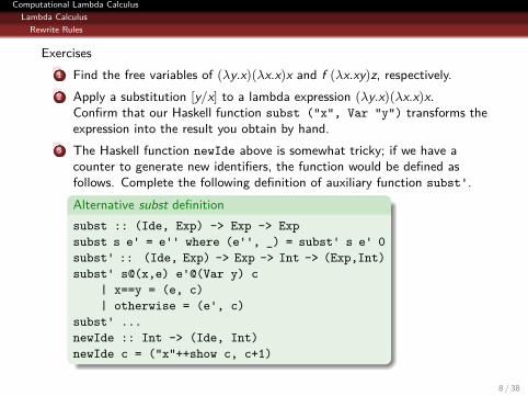
Exercises...1 Find the free variables of (λy.x)(λx.x)x and f (λx.xy)z, respectively....2 Apply a substitution [y/x] to a lambda expression (λy.x)(λx.x)x.

Confirm that our Haskell function subst ("x", Var "y") transforms theexpression into the result you obtain by hand.

...3 The Haskell function newIde above is somewhat tricky; if we have acounter to generate new identifiers, the function would be defined asfollows. Complete the following definition of auxiliary function subst'..Alternative subst definition..

.

. ..

.

.

subst :: (Ide, Exp) -> Exp -> Expsubst s e' = e'' where (e'', _) = subst' s e' 0subst' :: (Ide, Exp) -> Exp -> Int -> (Exp,Int)subst' s@(x,e) e'@(Var y) c

| x==y = (e, c)| otherwise = (e', c)

subst' ...newIde :: Int -> (Ide, Int)newIde c = ("x"++show c, c+1)

8 / 38


Convertibility and Reducibility

Convertibility under Rewrite Rules

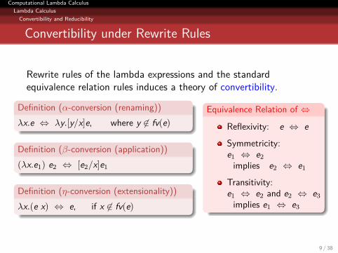
Rewrite rules of the lambda expressions and the standardequivalence relation rules induces a theory of convertibility.

.Definition (α-conversion (renaming)).... ..

.

.λx.e ⇔ λy.[y/x]e, where y ∈ fv(e)

.Definition (β-conversion (application)).... ..

.

.(λx.e1) e2 ⇔ [e2/x]e1

.Definition (η-conversion (extensionality)).... ..

..λx.(e x) ⇔ e, if x ∈ fv(e)

.Equivalence Relation of ⇔..

.. ..

.

.

Reflexivity: e ⇔ eSymmetricity:e1 ⇔ e2

implies e2 ⇔ e1Transitivity:e1 ⇔ e2 and e2 ⇔ e3

implies e1 ⇔ e3

9 / 38



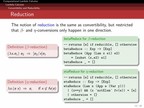
ReductionThe notion of reduction is the same as convertibility, but restrictedthat β- and η-conversions only happen in one direction.

.Definition (β-reduction).... ..

.

.(λx.e1) e2 ⇒ [e2/x]e1

.betaReduce for β-reduction

..

.

. ..

.

.

-- returns [e] if reducible, [] otherwisebetaReduce :: Exp -> [Exp]betaReduce (App (Lam x e1) e2)

= [subst (x,e2) e1]betaReduce _ = []

.Definition (η-reduction).... ..

.

.λx.(e x) ⇒ e, if x ∈ fv(e)

.etaReduce for η-reduction

..

.

. ..

.

.

-- returns [e] if reducible, [] otherwiseetaReduce :: Exp -> [Exp]etaReduce (Lam x (App e (Var y)))| (x==y) && (x `notElem` fv(e)) = [e]| otherwise = []

etaReduce _ = []

10 / 38



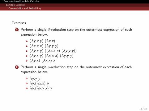
Exercises...1 Perform a single β-reduction step on the outermost expression of each

expression below.(λy.x y) (λx.x)(λx.x x) (λy.y y)(λy.x y) ((λx.x x) (λy.y y))(λy.x y) (λx.x x) (λy.y y)(λy.x) (λx.x) x

...2 Perform a single η-reduction step on the outermost expression of eachexpression below.

λy.y yλy.(λx.x) yλy.(λy.y x) y

11 / 38



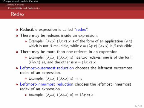
Redex

Reducible expression is called “redex”.There may be redexes inside an expression.

Example: (λy.x) (λx.x) x is of the form of an application (e x)which is not β-reducible, while e = (λy.x) (λx.x) is β-reducible.

There may be more than one redexes in an expression.Example: (λy.x) ((λx.x) x) has two redexes; one is of the form((λy.x) e), and the other is e = (λx.x) x.

Leftmost-outermost reduction chooses the leftmost outermostredex of an expression.

Example: (λy.x) ((λx.x) x) ⇒ xLeftmost-innermost reduction chooses the leftmost innermostredex of an expression.

Example: (λy.x) ((λx.x) x) ⇒ (λy.x) x

12 / 38



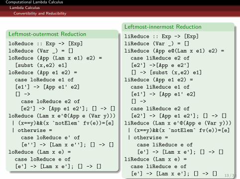
.Leftmost-outermost Reduction..

.

. ..

.

.

loReduce :: Exp -> [Exp]loReduce (Var _) = []loReduce (App (Lam x e1) e2) =[subst (x,e2) e1]

loReduce (App e1 e2) =case loReduce e1 of[e1'] -> [App e1' e2][] ->case loReduce e2 of[e2'] -> [App e1 e2']; [] -> []

loReduce (Lam x e'@(App e (Var y)))| (x==y)&&(x `notElem` fv(e))=[e]| otherwise =

case loReduce e' of[e''] -> [Lam x e'']; [] -> []

loReduce (Lam x e) =case loReduce e of[e'] -> [Lam x e']; [] -> []

.Leftmost-innermost Reduction..

.

. ..

.

.

liReduce :: Exp -> [Exp]liReduce (Var _) = []liReduce (App e@(Lam x e1) e2) =

case liReduce e2 of[e2'] ->[App e e2'][] -> [subst (x,e2) e1]

liReduce (App e1 e2) =case liReduce e1 of[e1'] -> [App e1' e2][] ->case liReduce e2 of[e2'] -> [App e1 e2']; [] -> []

liReduce (Lam x e'@(App e (Var y)))| (x==y)&&(x `notElem` fv(e))=[e]| otherwise =

case liReduce e of[e'] -> [Lam x e']; [] -> []

liReduce (Lam x e) =case liReduce e of[e'] -> [Lam x e']; [] -> [] 13 / 38



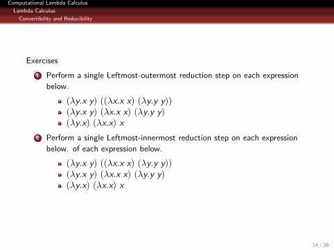
Exercises...1 Perform a single Leftmost-outermost reduction step on each expression

below.(λy.x y) ((λx.x x) (λy.y y))(λy.x y) (λx.x x) (λy.y y)(λy.x) (λx.x) x

...2 Perform a single Leftmost-innermost reduction step on each expressionbelow. of each expression below.

(λy.x y) ((λx.x x) (λy.y y))(λy.x y) (λx.x x) (λy.y y)(λy.x) (λx.x) x

14 / 38




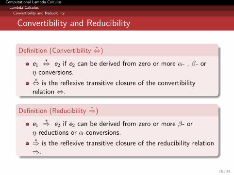
.Definition (Convertibility ∗⇔)..

.. ..

.

.

e1 ∗⇔ e2 if e2 can be derived from zero or more α- , β- orη-conversions.∗⇔ is the reflexive transitive closure of the convertibility

relation ⇔..Definition (Reducibility ∗⇒)..

.. ..

.

.

e1 ∗⇒ e2 if e2 can be derived from zero or more β- orη-reductions or α-conversions.∗⇒ is the reflexive transitive closure of the reducibility relation⇒.

15 / 38



Normal Form

.Definition (Normal form)..

.. ..

.

.

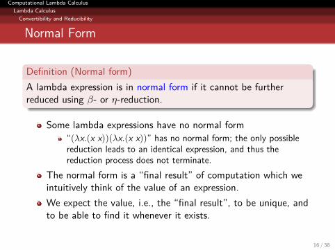
A lambda expression is in normal form if it cannot be furtherreduced using β- or η-reduction.

Some lambda expressions have no normal form“(λx.(x x))(λx.(x x))” has no normal form; the only possiblereduction leads to an identical expression, and thus thereduction process does not terminate.

The normal form is a “final result” of computation which weintuitively think of the value of an expression.We expect the value, i.e., the “final result”, to be unique, andto be able to find it whenever it exists.

16 / 38


Church-Rosser Theorem

Church-Rosser Theorem.Theorem (Church-Rosser Theorem I).... ..

.

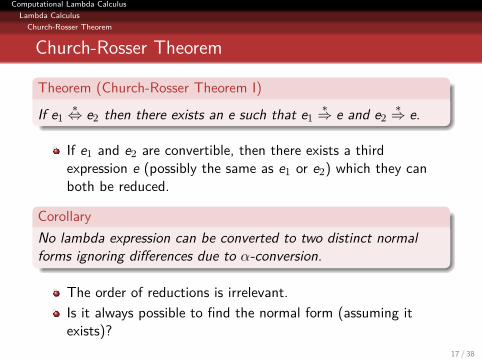
.If e1 ∗⇔ e2 then there exists an e such that e1 ∗⇒ e and e2 ∗⇒ e.

If e1 and e2 are convertible, then there exists a thirdexpression e (possibly the same as e1 or e2) which they canboth be reduced.

.Corollary..

.. ..

.

.

No lambda expression can be converted to two distinct normalforms ignoring differences due to α-conversion.

The order of reductions is irrelevant.Is it always possible to find the normal form (assuming itexists)?

17 / 38


Reduction Strategies

Normal-order and Applicative-order Reductions

.Definition (Normal-order Reduction)..

.. ..

.

.

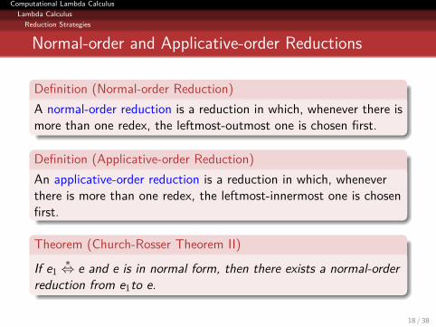
A normal-order reduction is a reduction in which, whenever there ismore than one redex, the leftmost-outmost one is chosen first..Definition (Applicative-order Reduction)..

.. ..

.

.

An applicative-order reduction is a reduction in which, wheneverthere is more than one redex, the leftmost-innermost one is chosenfirst..Theorem (Church-Rosser Theorem II)..

.. ..

.

.

If e1 ∗⇔ e and e is in normal form, then there exists a normal-orderreduction from e1to e.

18 / 38


Reduction Strategies

.Normal-order and Applicative-order reductions

..

.

. ..

.

.

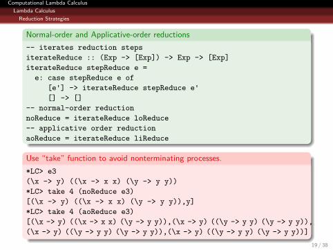
-- iterates reduction stepsiterateReduce :: (Exp -> [Exp]) -> Exp -> [Exp]iterateReduce stepReduce e =e: case stepReduce e of

[e'] -> iterateReduce stepReduce e'[] -> []

-- normal-order reductionnoReduce = iterateReduce loReduce-- applicative order reductionaoReduce = iterateReduce liReduce

.Use “take” function to avoid nonterminating processes.

..

.

. ..

.

.

*LC> e3(\x -> y) ((\x -> x x) (\y -> y y))*LC> take 4 (noReduce e3)[(\x -> y) ((\x -> x x) (\y -> y y)),y]*LC> take 4 (aoReduce e3)[(\x -> y) ((\x -> x x) (\y -> y y)),(\x -> y) ((\y -> y y) (\y -> y y)),(\x -> y) ((\y -> y y) (\y -> y y)),(\x -> y) ((\y -> y y) (\y -> y y))]

19 / 38


Recursion, Lambda-definability and Church’s Thesis

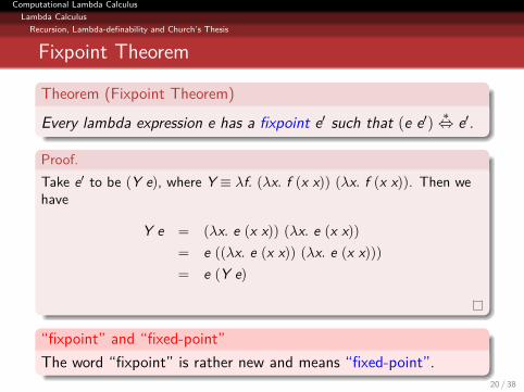
Fixpoint Theorem.Theorem (Fixpoint Theorem).... ..

.

.Every lambda expression e has a fixpoint e′ such that (e e′) ∗⇔ e′..Proof...

.. ..

.

.

Take e′ to be (Y e), where Y ≡ λf. (λx. f (x x)) (λx. f (x x)). Then wehave

Y e = (λx. e (x x)) (λx. e (x x))= e ((λx. e (x x)) (λx. e (x x)))= e (Y e)

.“fixpoint” and “fixed-point”..

.. ..

.

.The word “fixpoint” is rather new and means “fixed-point”.20 / 38



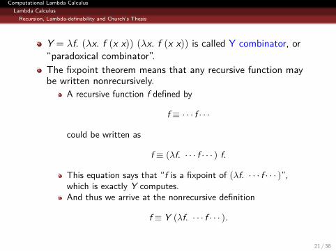
Y = λf. (λx. f (x x)) (λx. f (x x)) is called Y combinator, or“paradoxical combinator”.The fixpoint theorem means that any recursive function maybe written nonrecursively.

A recursive function f defined by

f ≡ · · · f · · ·

could be written as

f ≡ (λf. · · · f · · · ) f.

This equation says that “f is a fixpoint of (λf. · · · f · · · )”,which is exactly Y computes.And thus we arrive at the nonrecursive definition

f ≡ Y (λf. · · · f · · · ).

21 / 38



Church’s Thesis

.Church’s Thesis..

.. ..

.

.

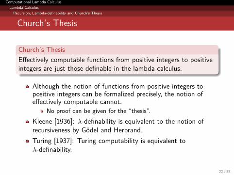
Effectively computable functions from positive integers to positiveintegers are just those definable in the lambda calculus.

Although the notion of functions from positive integers topositive integers can be formalized precisely, the notion ofeffectively computable cannot.

No proof can be given for the “thesis”.Kleene [1936]: λ-definability is equivalent to the notion ofrecursiveness by Godel and Herbrand.Turing [1937]: Turing computability is equivalent toλ-definability.

22 / 38



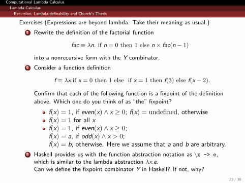
Exercises (Expressions are beyond lambda. Take their meaning as usual.)...1 Rewrite the definition of the factorial function

fac ≡ λn. if n = 0 then 1 else n × fac(n − 1)

into a nonrecursive form with the Y combinator....2 Consider a function definition

f ≡ λx.if x = 0 then 1 else if x = 1 then f(3) else f(x − 2).

Confirm that each of the following function is a fixpoint of the definitionabove. Which one do you think of as “the” fixpoint?

f(x) = 1, if even(x) ∧ x ≥ 0; f(x) = undefined, otherwisef(x) = 1 for all xf(x) = 1, if even(x) ∧ x ≥ 0;f(x) = a, if odd(x) ∧ x > 0;f(x) = b, otherwise. Here we assume that a and b are arbitrary.

...3 Haskell provides us with the function abstraction notation as \x -> e,which is similar to the lambda abstraction λx.e.Can we define the fixpoint combinator Y in Haskell? If not, why?

23 / 38


Encoding Booleans and Numbers

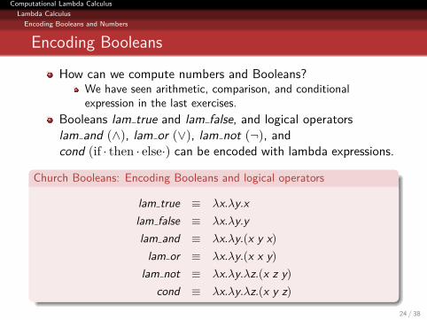
Encoding BooleansHow can we compute numbers and Booleans?

We have seen arithmetic, comparison, and conditionalexpression in the last exercises.

Booleans lam true and lam false, and logical operatorslam and (∧), lam or (∨), lam not (¬), andcond (if · then · else·) can be encoded with lambda expressions.

.Church Booleans: Encoding Booleans and logical operators..

.. ..

.

.

lam true ≡ λx.λy.xlam false ≡ λx.λy.ylam and ≡ λx.λy.(x y x)

lam or ≡ λx.λy.(x x y)lam not ≡ λx.λy.λz.(x z y)

cond ≡ λx.λy.λz.(x y z)24 / 38



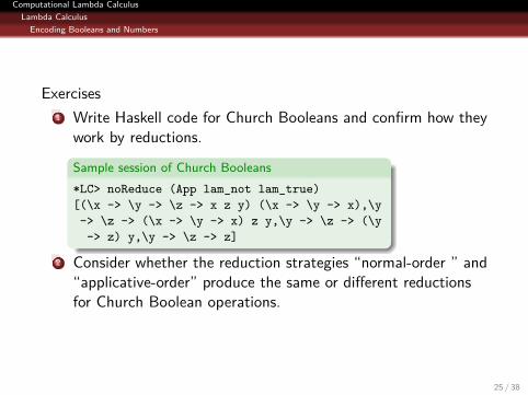
Exercises...1 Write Haskell code for Church Booleans and confirm how they

work by reductions..Sample session of Church Booleans..

.

. ..

.

.

*LC> noReduce (App lam_not lam_true)[(\x -> \y -> \z -> x z y) (\x -> \y -> x),\y-> \z -> (\x -> \y -> x) z y,\y -> \z -> (\y-> z) y,\y -> \z -> z]

...2 Consider whether the reduction strategies “normal-order ” and“applicative-order” produce the same or different reductionsfor Church Boolean operations.

25 / 38



Encoding Natural Numbers

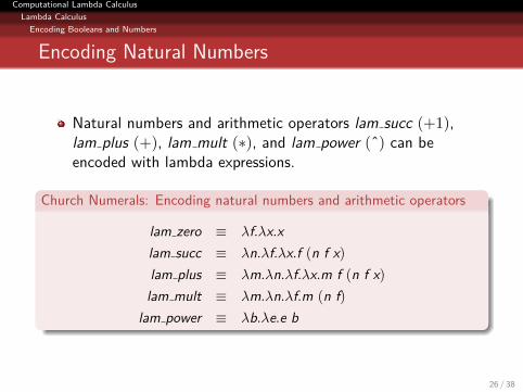
Natural numbers and arithmetic operators lam succ (+1),lam plus (+), lam mult (∗), and lam power (ˆ) can beencoded with lambda expressions.

.Church Numerals: Encoding natural numbers and arithmetic operators..

.. ..

.

.

lam zero ≡ λf.λx.xlam succ ≡ λn.λf.λx.f (n f x)lam plus ≡ λm.λn.λf.λx.m f (n f x)lam mult ≡ λm.λn.λf.m (n f)

lam power ≡ λb.λe.e b

26 / 38



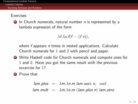
Exercises...1 In Church numerals, natural number n is represented by a

lambda expression of the form

λf.λx.f(f · · · (f x)),

where f appears n times in nested applications. CalculateChurch numerals for 1 and 2 with pencil and paper.

...2 Write Haskell code for Church numerals and compute ones for1 and 2. Have you got the same result with the previousexcercise for 1?

...3 Prove that

lam plus = λm.λn.m lam succ n, andlam mult = λm.λn.m (lam plus n) lam zero

27 / 38


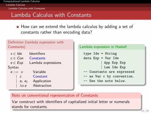
Lambda Calculus with Constants


How can we extend the lambda calculus by adding a set ofconstants rather than encoding data?

.Definition (lambda expression withConstants)..

.

. ..

.

.

x ∈ Ide Identifiersc ∈ Con Constantse ∈ Exp Lambda expressions

Syntaxe ::= x Variable

| c Constant| e1 e2 Application| λx.e Abstraction

.Lambda expression in Haskell

..

.

. ..

.

.

type Ide = Stringdata Exp = Var Ide

| App Exp Exp| Lam Ide Exp

-- Constants are expressed-- as Var c by convention.-- See the note below.

.Note on conventional representation of Constants..

.. ..

.

.

Var construct with identifiers of capitalized initial letter or numeralsstands for constants.

28 / 38



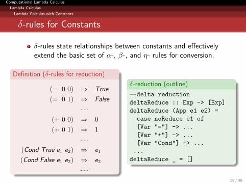
δ-rules for Constants

δ-rules state relationships between constants and effectivelyextend the basic set of α-, β-, and η- rules for conversion.

.Definition (δ-rules for reduction)..

.. ..

.

.

(= 0 0) ⇒ True(= 0 1) ⇒ False

· · ·(+ 0 0) ⇒ 0

(+ 0 1) ⇒ 1

· · ·(Cond True e1 e2) ⇒ e1(Cond False e1 e2) ⇒ e2

· · ·

.δ-reduction (outline)..

.. ..

.

.

--delta reductiondeltaReduce :: Exp -> [Exp]deltaReduce (App e1 e2) =

case noReduce e1 of[Var "="] -> ...[Var "+"] -> ...[Var "Cond"] -> ...

...deltaReduce _ = []

29 / 38

Computational Lambda CalculusCombinator Calculus

Combinators

Combinators

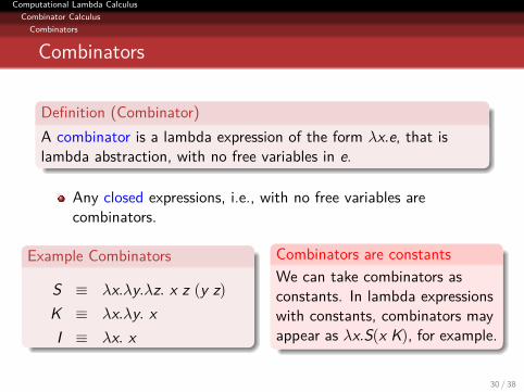
.Definition (Combinator)..

.. ..

.

.

A combinator is a lambda expression of the form λx.e, that islambda abstraction, with no free variables in e.

Any closed expressions, i.e., with no free variables arecombinators.

.Example Combinators..

.. ..

..

S ≡ λx.λy.λz. x z (y z)K ≡ λx.λy. xI ≡ λx. x

.Combinators are constants..

.. ..

.

.

We can take combinators asconstants. In lambda expressionswith constants, combinators mayappear as λx.S(x K), for example.

30 / 38


Combinators

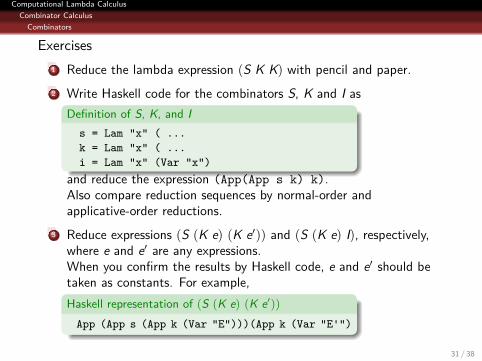
Exercises...1 Reduce the lambda expression (S K K) with pencil and paper....2 Write Haskell code for the combinators S, K and I as

.Definition of S, K, and I..

.

. ..

.

.

s = Lam "x" ( ...k = Lam "x" ( ...i = Lam "x" (Var "x")

and reduce the expression (App(App s k) k).Also compare reduction sequences by normal-order andapplicative-order reductions.

...3 Reduce expressions (S (K e) (K e′)) and (S (K e) I), respectively,where e and e′ are any expressions.When you confirm the results by Haskell code, e and e′ should betaken as constants. For example,.Haskell representation of (S (K e) (K e′)).... ..

.

.App (App s (App k (Var "E")))(App k (Var "E'")

31 / 38


Combinators

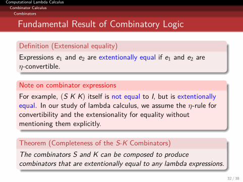
Fundamental Result of Combinatory Logic.Definition (Extensional equality)..

.. ..

.

.

Expressions e1 and e2 are extentionally equal if e1 and e2 areη-convertible.

.Note on combinator expressions..

.. ..

.

.

For example, (S K K) itself is not equal to I, but is extentionallyequal. In our study of lambda calculus, we assume the η-rule forconvertibility and the extensionality for equality withoutmentioning them explicitly.

.Theorem (Completeness of the S-K Combinators)..

.. ..

.

.

The combinators S and K can be composed to producecombinators that are extentionally equal to any lambda expressions.

32 / 38


Combinators

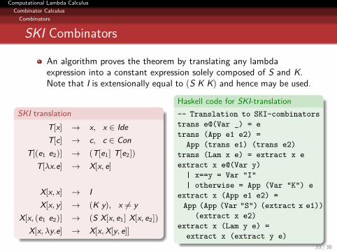
SKI Combinators

An algorithm proves the theorem by translating any lambdaexpression into a constant expression solely composed of S and K.Note that I is extensionally equal to (S K K) and hence may be used.

.SKI translation..

.

. ..

.

.

T[x] → x, x ∈ IdeT[c] → c, c ∈ Con

T[(e1 e2)] → (T[e1] T[e2])T[λx.e] → X[x, e]

X[x, x] → IX[x, y] → (K y), x = y

X[x, (e1 e2)] → (S X[x, e1] X[x, e2])X[x, λy.e] → X[x,X[y, e]]

.Haskell code for SKI-translation..

.

. ..

.

.

-- Translation to SKI-combinatorstrans e@(Var _) = etrans (App e1 e2) =App (trans e1) (trans e2)

trans (Lam x e) = extract x eextract x e@(Var y)| x==y = Var "I"| otherwise = App (Var "K") e

extract x (App e1 e2) =App (App (Var "S") (extract x e1))

(extract x e2)extract x (Lam y e) =extract x (extract y e)

33 / 38


Combinators

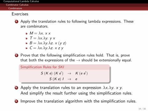
Exercises...1 Apply the translation rules to following lambda expressions. These

are combinators.M = λx. x xT = λx.λy. y xB = λx.λy.λz. x (y z)C = λx.λy.λz. x z y

...2 Prove that the following simplification rules hold. That is, provethat both the expressions of the → should be extensionally equal..Simplification Rules for SKI..

.

. ..

.

.

S (K e) (K e′) → K (e e′)S (K e) I → e

...3 Apply the translation rules to an expression λx.λy. x y.And simplify the result further using the simplification rules.

...4 Improve the translation algorithm with the simplification rules.34 / 38


Combinators

SKIBC Combinators

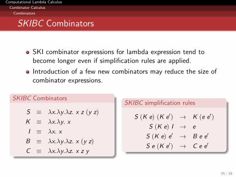
SKI combinator expressions for lambda expression tend tobecome longer even if simplification rules are applied.Introduction of a few new combinators may reduce the size ofcombinator expressions.

.SKIBC Combinators..

.. ..

.

.S ≡ λx.λy.λz. x z (y z)K ≡ λx.λy. xI ≡ λx. x

B ≡ λx.λy.λz. x (y z)C ≡ λx.λy.λz. x z y

.SKIBC simplification rules..

.. ..

.

.

S (K e) (K e′) → K (e e′)S (K e) I → e

S (K e) e′ → B e e′

S e (K e′) → C e e′

35 / 38


Combinators

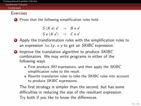
Exercises...1 Prove that the following simplification rules hold.

S (K e) e′ → B e e′

S e (K e′) → C e e′...2 Apply the transformation rules with the simplification rules to

an expression λx.λy. x y to get an SKIBC expression....3 Improve the translation algorithm to produce SKIBC

combinators. We may write programs in either of thefollowing ways.

First produce SKI expressions, and then apply the SKIBCsimplification rules to the result.Rewrite translation rules to take the SKIBC rules into accountto produce SKIBC expressions.

The first strategy is simpler than the second, but has somedifficulties in reducing the size of the resultant expression.Try both if you like to know the differences.

36 / 38


Combinators

Combinator Reduction

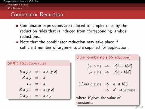
Combinator expressions are reduced to simpler ones by thereduction rules that is induced from corresponding lambdareductions.Note that the combinator reduction may take place ifsufficient number of arguments are supplied for application.

.SKIBC Reduction rules..

.. ..

..

S x y z ⇒ x z (y z)K x y ⇒ x

I x ⇒ xB x y z ⇒ x (y z)C x y z ⇒ x z y

.Other combinators (δ-reduction)..

.. ..

.

.

(+ e e′) ⇒ V[e] + V[e′](∗ e e′) ⇒ V[e] ∗ V[e′]

(Cond b e e′) ⇒ e , if V[b]⇒ e′ , otherwise

where V gives the value ofconstants.

37 / 38


Combinators

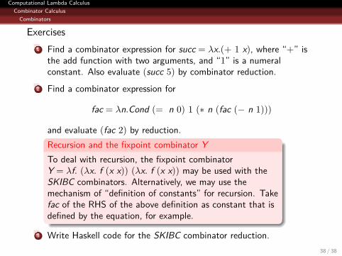
Exercises...1 Find a combinator expression for succ = λx.(+ 1 x), where “+” is

the add function with two arguments, and “1” is a numeralconstant. Also evaluate (succ 5) by combinator reduction.

...2 Find a combinator expression for

fac = λn.Cond (= n 0) 1 (∗ n (fac (− n 1)))

and evaluate (fac 2) by reduction..Recursion and the fixpoint combinator Y..

.. ..

.

.

To deal with recursion, the fixpoint combinatorY = λf. (λx. f (x x)) (λx. f (x x)) may be used with theSKIBC combinators. Alternatively, we may use themechanism of “definition of constants” for recursion. Takefac of the RHS of the above definition as constant that isdefined by the equation, for example.

...3 Write Haskell code for the SKIBC combinator reduction.38 / 38

Documents

Lambda Calculus CLC