Lake Water Quality Model with Focus on Cyanobacteria · cyanobacteria, the physical and chemical characteristics of the environment that cause ... simulates or does not simulate each

Lake Water Quality Model with Focus on Cyanobacteria Theresa McGovern

ENSR 2 Technology Park Drive

Westford Massachusetts 01886 Work performed at Tufts University, Medford Massachusetts

ABSTRACT The cause of cyanobacteria’s growth and dominance in certain eutrophic lakes is explored via a water quality model application. The one-dimensional lake water quality model includes nitrogen, phosphorus, silica, three phytoplankton groups and zooplankton. Lake Washington was used as the case study due to its unique history of eutrophication during a large wastewater nutrient loading period from in the 1960s and subsequent recovery. Sampling data for a 20-year period surrounding the eutrophication includes speciation of phytoplankton. Results indicate that nutrient loading, specifically phosphorus was the main factor for the persistent dominance of Oscillatoria in Lake Washington. Other key conditions and cyanobacteria traits are analyzed and discussed. KEYWORDS Cyanobacteria, blue-greens, phytoplankton, water quality model, eutrophication INTRODUCTION Eutrophication, or heightened biological production, in water bodies is a problem and concern due to nutrient-rich runoff and inflow. Eutrophication causes reduced clarity, reduced dissolved oxygen and taste and odor problems in water bodies. Efforts have been made to describe the nutrient cycles, their relation to phytoplankton and plant growth, and the overall effect of nutrient input on river and lake systems. This knowledge is important for decision-making on several levels including lake management and discharge permitting. Blue-green algae, or cyanobacteria, are contributors to eutrophication that stand out because of their special characteristics. Technically classified under the bacteria domain, they are often grouped with phytoplankton for water quality analysis. Different species of cyanobacteria are capable of living in a wide range of climate and trophic conditions. They are prokaryotic organisms (cells containing no nucleus) that were the dominant forms of life on the Earth over 1.5 billion years ago and were the first organisms to produce oxygen and chlorophylls a and b (Graham and Wilcox 2000). Some species are used as human food sources including health foods high in vitamins and proteins. Other species are used as fertilizers in rice fields because of their ability to fix atmospheric nitrogen. Although there are some beneficial uses to species of cyanobacteria, they are considered a nuisance group in lake ecosystems. Specifically, cyanobacteria are most commonly associated with blooms in highly eutrophic systems late in summer. They are considered a problem because, according to Paerl (1988), bloom-forming phytoplankton (blue-greens) can cause perceptible water quality deterioration, heath hazards, or losses of aesthetic and recreational value. Some cyanobacteria are toxic to animals and people when ingested. They often create an unattractive, odorous coating on the water’s surface that requires additional treatment when

3910

WEFTEC®.06

Copyright 2006 Water Environment Foundation. All Rights Reserved©

present in drinking water systems. When conditions are favorable for their growth, cyanobacteria tend to dominate instead of co-existing with other phytoplankton groups. Special research interest in cyanobacteria is the result of their significantly different growth and survival characteristics. Previous work includes studies and experiments defining cyanobacteria characteristics, regression analysis correlating cyanobacteria growth with physical and chemical lake characteristics, and models that simulate cyanobacteria separately from other phytoplankton. Despite this work, agreement of the causes of cyanobacteria growth and dominance does not exist among experts. This research combines knowledge of cyanobacteria with practical modeling techniques to simulate their growth and dominance. Specific causes of cyanobacteria growth are explored through the simulation of a large bloom. A water quality model was created including nutrient and phytoplankton groups as state variables. Cyanobacteria were modeled separately than other phytoplankton groups to distinguish their special characteristics and establish modeling techniques capable of accurate simulation. The model was tested against a 20-year period of water quality in Lake Washington, which experienced a recurrent cyanobacteria bloom in the 1960s that disappeared and has not resurfaced since. This data set allows the model to be tested against both long-term trends and seasonal cycles of nutrients and phytoplankton during cyanobacteria’s presence and absence. Also, periods of cyanobacteria high and low growth are included to fully test the modeling techniques. The benefit of this computer model is the ability to include several potential influences on cyanobacterial growth and dominance at once. Cyanobacteria were modeled with individual rate coefficients and nutrient needs. In this way, the factors that affect cyanobacteria growth can be quantitatively determined and tested. This paper first summarizes current knowledge of cyanobacteria’s unique characteristics in the context of current dominance theories. These ideas form the basis of the modeling techniques used to simulate cyanobacteria differently than other phytoplankton groups. The lake water quality model is then described including mathematical equations. The model is applied to Lake Washington’s water quality history. The results are discussed in regard to the successful and not successful techniques of cyanobacteria simulation taken from the literature. The goal of this work is to identify characteristics that can be used in a modeling framework to accurately simulate cyanobacteria growth.

3911

WEFTEC®.06


LITERATURE REVIEW The literature was reviewed to identify previous work concerning the characteristics of cyanobacteria, the physical and chemical characteristics of the environment that cause cyanobacteria growth, and the modeling techniques used to simulate their growth. The insight gained from previous work guided the model construction and calibration. A full literature review is presented in McGovern, 2005 and the following is a summary of relevant findings. Cyanobacteria Characteristics Cyanobacteria possess characteristics different than other groups of phytoplankton. These characteristics have been studied both in the laboratory and in the field. They form the basis of current theories of why blooms occur and why this group can dominate. These characteristics can be incorporated into the model through the cyanobacteria’s interactions with the other state variables including the nutrients and zooplankton. Specifically, rate coefficients and parameters associated with cyanobacteria can be set to represent these characteristics. The following is a list their characteristics with an explanation of how the model simulates or does not simulate each (not in order of importance).

• Toxic or undesirable to zooplankton grazers. In the model, the cyanobacteria have no

grazing losses to represent these findings. • Able to regulate buoyancy, possibly giving them optimal light and nutrients in addition to

shading other phytoplankton and avoiding sedimentation. This model simulate losses due to settling (or lack of this loss), but as explained in the results, giving cyanobacteria access to more light and nutrients was not necessary to obtain adequate results. The model is capable of setting an individual optimal light for the cyanobacteria phytoplankton group. This value can be set low to simulate their low light needs and utilization capabilities.

• Able to withstand high light conditions and grow under low light conditions. The model gave best result when cyanobacteria had an optimal light of 300 ly/d. Therefore, this trait does not prove highly influential in the Lake Washington case.

• Able to grow in high pH conditions. The model does not simulate pH and so the influence of slight variations were not tested, but also were not needed to explain the majority of the trends.

• Able to fix N2 (some species) and therefore out-compete other species when nitrogen is limiting (low N:P ratios). The dominant species in Lake Washington during the bloom period was the non-nitrogen fixing Oscillatoria and so nitrogen fixation was not tested with the model. This capability by other species could potentially be a large factor in their success and cannot be disregarded.

• Form symbiotic relationships with certain bacteria. This capability was not simulated in the model.

Environmental Conditions In addition to cyanobacteria’s unique characteristics, the surrounding environment possesses potential triggers for their growth that can be simulated and used to predict blooms. Research effort has been dedicated to determining these conditions that favor cyanobacteria dominance.

3912

WEFTEC®.06


The following factors, summarized from Paerl (2001) unless otherwise noted, are included in the most current theories:

Turbulence – low levels of non-disruptive mixing (50-100 rmp) have been shown to improve cyanobacteria growth by cycling nutrients, although strong mixing begins to inhibit growth. Strong mixing has been shown specifically to reduce nitrogen fixation in Anabaena oscillarioides. In addition, turbulence breaks up surface scums and increases CO2, eliminating their advantage (see 2.1.4 above). Edmondson (1997) showed that higher wind velocities were the main factor contributing to the 1988 bloom of Aphanizomenon in Lake Washington.

High temperatures – cyanobacteria have higher optimal temperatures for growth. Water column stratification – vertical stratification allows cyanobacteria to persist at a

depth that has optimal conditions for growth in addition to obtaining CO2 directly from the surface when CO2 is limited.

Trace elements – elements can be limiting for growth, although it is less common than nutrient limitation. Iron, manganese, zinc, cobalt, copper are needed for photosynthesis and nitrogen fixation.

Salinity – freshwater species may be inhibited by high levels of salinity although there are several examples of estuarine and marine species of cyanobacteria.

In addition to all of these factors and characteristics, cyanobacteria can form resting cells called akinetes that remain dormant during poor growth conditions. They have the ability to remain in sediments and even soil until favorable growth conditions return. (Paerl 1988) The model includes a temperature simulation and temperature affects on cyanobacteria growth. In addition, thermal stratification is simulated through vertical dispersion coefficients. Trace element limitation, salinity limitation, or turbulence effects on growth are not included in the model. The success of the model indicates that these omitted conditions are not major influences on cyanobacteria, for at least this case.

3913

WEFTEC®.06


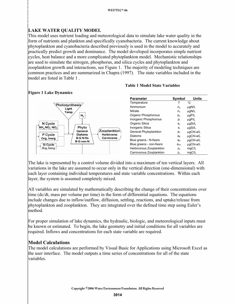
LAKE WATER QUALITY MODEL This model uses nutrient loading and meteorological data to simulate lake water quality in the form of nutrients and plankton and specifically cyanobacteria. The current knowledge about phytoplankton and cyanobacteria described previously is used in the model to accurately and practically predict growth and dominance. The model developed incorporates simple nutrient cycles, heat balance and a more complicated phytoplankton model. Mechanistic relationships are used to simulate the nitrogen, phosphorus, and silica cycles and phytoplankton and zooplankton growth and interactions, see Figure 1. The majority of modeling techniques are common practices and are summarized in Chapra (1997). The state variables included in the model are listed in Table 1 . Table 1 Model State Variables

Figure 1 Lake Dynamics Parameter Symbol Units Temperature T °C Ammonium na μgN/L Nitrate nn μgN/L Organic Phosphorous po μgP/L Inorganic Phosphorous pi μgP/L Organic Silica so μgSi/L Inorganic Silica si μgSi/L General Phytoplankton a7 μgChl-a/L Diatoms a8 μgChl-a/L Blue greens - N-fixers a9 μgChl-a/L Blue greens - non-fixers a10 μgChl-a/L Herbivorous Zooplankton zh mgC/L Carnivorous Zooplankton zc mgC/L

The lake is represented by a control volume divided into a maximum of ten vertical layers. All variations in the lake are assumed to occur only in the vertical direction (one-dimensional) with each layer containing individual temperatures and state variable concentrations. Within each layer, the system is assumed completely mixed. All variables are simulated by mathematically describing the change of their concentrations over time (dc/dt, mass per volume per time) in the form of differential equations. The equations include changes due to inflow/outflow, diffusion, settling, reactions, and uptake/release from phytoplankton and zooplankton. They are integrated over the defined time step using Euler’s method. For proper simulation of lake dynamics, the hydraulic, biologic, and meteorological inputs must be known or estimated. To begin, the lake geometry and initial conditions for all variables are required. Inflows and concentrations for each state variable are required. Model Calculations The model calculations are performed by Visual Basic for Applications using Microsoft Excel as the user interface. The model outputs a time series of concentrations for all of the state variables.

Organic Nitrogen

3914

WEFTEC®.06


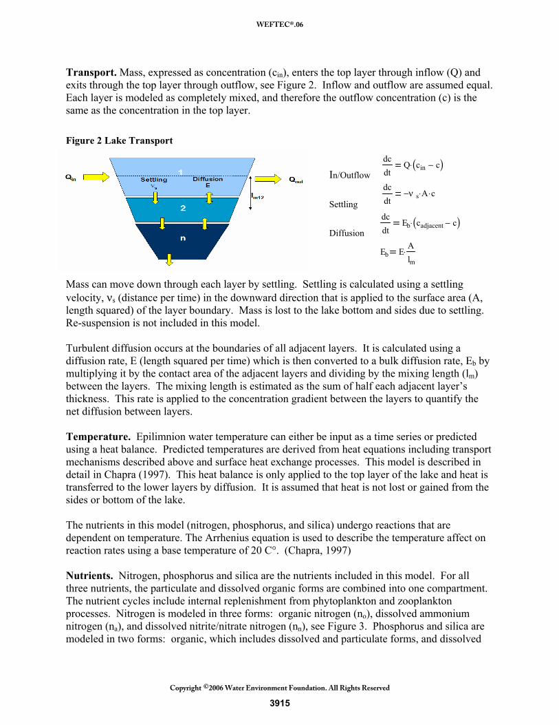
Transport. Mass, expressed as concentration (cin), enters the top layer through inflow (Q) and exits through the top layer through outflow, see Figure 2. Inflow and outflow are assumed equal. Each layer is modeled as completely mixed, and therefore the outflow concentration (c) is the same as the concentration in the top layer.

Figure 2 Lake Transport

In/Outflow

dcdt

Q cin c−( )⋅

Settling

dcdt

ν s− A⋅ c⋅

Diffusion

dcdt

Eb cadjacent c−( )⋅

Eb E

Alm

⋅

Mass can move down through each layer by settling. Settling is calculated using a settling velocity, νs (distance per time) in the downward direction that is applied to the surface area (A, length squared) of the layer boundary. Mass is lost to the lake bottom and sides due to settling. Re-suspension is not included in this model. Turbulent diffusion occurs at the boundaries of all adjacent layers. It is calculated using a diffusion rate, E (length squared per time) which is then converted to a bulk diffusion rate, Eb by multiplying it by the contact area of the adjacent layers and dividing by the mixing length (lm) between the layers. The mixing length is estimated as the sum of half each adjacent layer’s thickness. This rate is applied to the concentration gradient between the layers to quantify the net diffusion between layers. Temperature. Epilimnion water temperature can either be input as a time series or predicted using a heat balance. Predicted temperatures are derived from heat equations including transport mechanisms described above and surface heat exchange processes. This model is described in detail in Chapra (1997). This heat balance is only applied to the top layer of the lake and heat is transferred to the lower layers by diffusion. It is assumed that heat is not lost or gained from the sides or bottom of the lake. The nutrients in this model (nitrogen, phosphorus, and silica) undergo reactions that are dependent on temperature. The Arrhenius equation is used to describe the temperature affect on reaction rates using a base temperature of 20 C°. (Chapra, 1997) Nutrients. Nitrogen, phosphorus and silica are the nutrients included in this model. For all three nutrients, the particulate and dissolved organic forms are combined into one compartment. The nutrient cycles include internal replenishment from phytoplankton and zooplankton processes. Nitrogen is modeled in three forms: organic nitrogen (no), dissolved ammonium nitrogen (na), and dissolved nitrite/nitrate nitrogen (nn), see Figure 3. Phosphorus and silica are modeled in two forms: organic, which includes dissolved and particulate forms, and dissolved

3915

WEFTEC®.06


inorganic available for phytoplankton use in photosynthesis (See Figure 4). Full nutrient processes are described further in McGovern (2005). Figure 3 Nitrogen Cycle Figure 4 Phosphorus and Silica Cycles Phytoplankton. Phytoplankton are modeled in four groups: diatoms, cyanobacteria capable of fixing atmospheric nitrogen, and cyanobacteria not capable of fixing atmospheric nitrogen, and general phytoplankton. Their transport, growth, and interactions are modeled the same, but unique rate coefficients represent their specific characteristics. All phytoplankton groups are expressed as concentrations of chlorophyll-a with a fixed internal stoichiometry including carbon, nitrogen, phosphorus, chlorophyll-a and silica for diatoms. In addition to transport and settling, phytoplankton grow via photosynthesis and are lost via respiration, death, and zooplankton grazing. Respiration is a process in which phytoplankton mass is released. The loss of phytoplankton due to respiration is modeled by a temperature-dependent respiration rate coefficient (kr, per day) multiplied by the phytoplankton concentration (a). As phytoplankton mass is release via respiration, nutrients are released and recycled back into the water column in proportion to the phytoplankton stoichiometry. Nutrients are recycled to both the organic and inorganic nitrogen pools based on a partitioning coefficient (0-1) that is calibrated to best match the data. The growth of phytoplankton via photosynthesis is modeled as a growth rate (kg, per day) multiplied by the concentration of phytoplankton (a). The optimal growth rate (kgopt) is input by the user and this rate is decreased by factors (φ) that range from zero to one and relate temperature (T), light (L), and nutrient (N) limitations. These factors are assumed to act independently.

kg kgopt φT⋅ φL⋅ φN⋅

Temperature This model simulates temperature limitation affects (φT) with an optimal temperature mode that allows for a different limiting relationship when the temperature is either below optimal or above optimal. When using this method, the optimal temperature and slope coefficients (κ) are calibrated to match the growth patterns of the phytoplankton.

3916

WEFTEC®.06


φT eκ 1− T Topt−( )2⋅

T Topt≤ φT e

κ 2− Topt T−( )2⋅ T Topt>

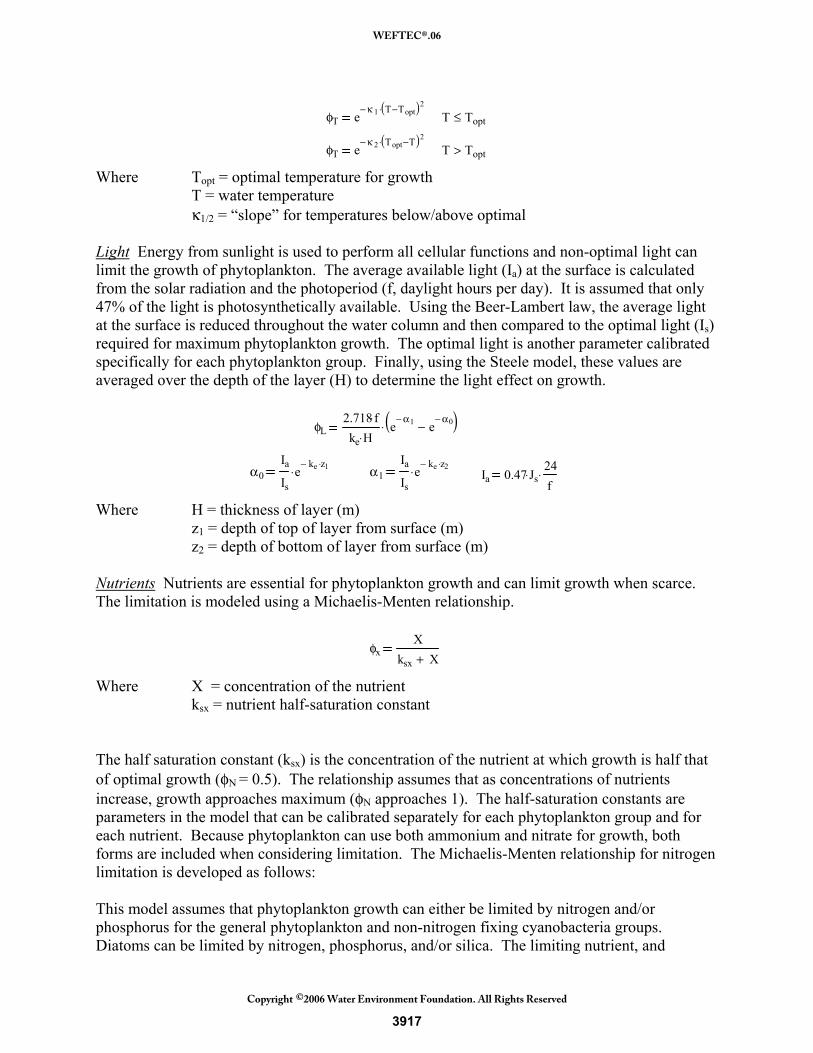
Where Topt = optimal temperature for growth T = water temperature κ1/2 = “slope” for temperatures below/above optimal Light Energy from sunlight is used to perform all cellular functions and non-optimal light can limit the growth of phytoplankton. The average available light (Ia) at the surface is calculated from the solar radiation and the photoperiod (f, daylight hours per day). It is assumed that only 47% of the light is photosynthetically available. Using the Beer-Lambert law, the average light at the surface is reduced throughout the water column and then compared to the optimal light (Is) required for maximum phytoplankton growth. The optimal light is another parameter calibrated specifically for each phytoplankton group. Finally, using the Steele model, these values are averaged over the depth of the layer (H) to determine the light effect on growth.

φL2.718 f⋅ke H⋅

eα1−

eα0−

−( )⋅

α0Ia

Ise

ke− z1⋅⋅

α1

Ia

Ise

ke− z2⋅⋅

Ia 0.47 Js⋅

24f

⋅

Where H = thickness of layer (m) z1 = depth of top of layer from surface (m) z2 = depth of bottom of layer from surface (m) Nutrients Nutrients are essential for phytoplankton growth and can limit growth when scarce. The limitation is modeled using a Michaelis-Menten relationship.

φxX

ksx X+

Where X = concentration of the nutrient ksx = nutrient half-saturation constant

The half saturation constant (ksx) is the concentration of the nutrient at which growth is half that of optimal growth (φN = 0.5). The relationship assumes that as concentrations of nutrients increase, growth approaches maximum (φN approaches 1). The half-saturation constants are parameters in the model that can be calibrated separately for each phytoplankton group and for each nutrient. Because phytoplankton can use both ammonium and nitrate for growth, both forms are included when considering limitation. The Michaelis-Menten relationship for nitrogen limitation is developed as follows: This model assumes that phytoplankton growth can either be limited by nitrogen and/or phosphorus for the general phytoplankton and non-nitrogen fixing cyanobacteria groups. Diatoms can be limited by nitrogen, phosphorus, and/or silica. The limiting nutrient, and

3917

WEFTEC®.06


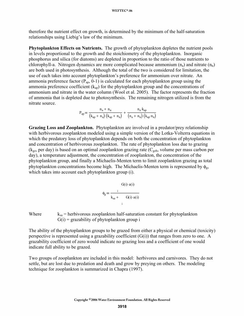
therefore the nutrient effect on growth, is determined by the minimum of the half-saturation relationships using Liebig’s law of the minimum. Phytoplankton Effects on Nutrients. The growth of phytoplankton depletes the nutrient pools in levels proportional to the growth and the stoichiometry of the phytoplankton. Inorganic phosphorus and silica (for diatoms) are depleted in proportion to the ratio of those nutrients to chlorophyll-a. Nitrogen dynamics are more complicated because ammonium (na) and nitrate (nn) are both used in photosynthesis. Although the total of the two is considered for limitation, the use of each takes into account phytoplankton’s preference for ammonium over nitrate. An ammonia preference factor (Pap, 0-1) is calculated for each phytoplankton group using the ammonia preference coefficient (kap) for the phytoplankton group and the concentrations of ammonium and nitrate in the water column (Wool et al. 2005). The factor represents the fraction of ammonia that is depleted due to photosynthesis. The remaining nitrogen utilized is from the nitrate source.

Papna nn+

kap na+( ) kap nn+( )⋅

na kap⋅

na nn+( ) kap nn⋅( )⋅+

Grazing Loss and Zooplankton. Phytoplankton are involved in a predator/prey relationship with herbivorous zooplankton modeled using a simple version of the Lotka-Volterra equations in which the predatory loss of phytoplankton depends on both the concentration of phytoplankton and concentration of herbivorous zooplankton. The rate of phytoplankton loss due to grazing (kgz, per day) is based on an optimal zooplankton grazing rate (Cgzh, volume per mass carbon per day), a temperature adjustment, the concentration of zooplankton, the concentration of the phytoplankton group, and finally a Michaelis-Menten term to limit zooplankton grazing as total phytoplankton concentrations become high. The Michaelis-Menten term is represented by φg, which takes into account each phytoplankton group (i).

φgi

G i( ) a i( )⋅

ksa

i

G i( ) a i( )⋅ +

Where ksa = herbivorous zooplankton half-saturation constant for phytoplankton G(i) = grazability of phytoplankton group i The ability of the phytoplankton groups to be grazed from either a physical or chemical (toxicity) perspective is represented using a grazability coefficient (G(i)) that ranges from zero to one. A grazability coefficient of zero would indicate no grazing loss and a coefficient of one would indicate full ability to be grazed. Two groups of zooplankton are included in this model: herbivores and carnivores. They do not settle, but are lost due to predation and death and grow by preying on others. The modeling technique for zooplankton is summarized in Chapra (1997).

3918

WEFTEC®.06


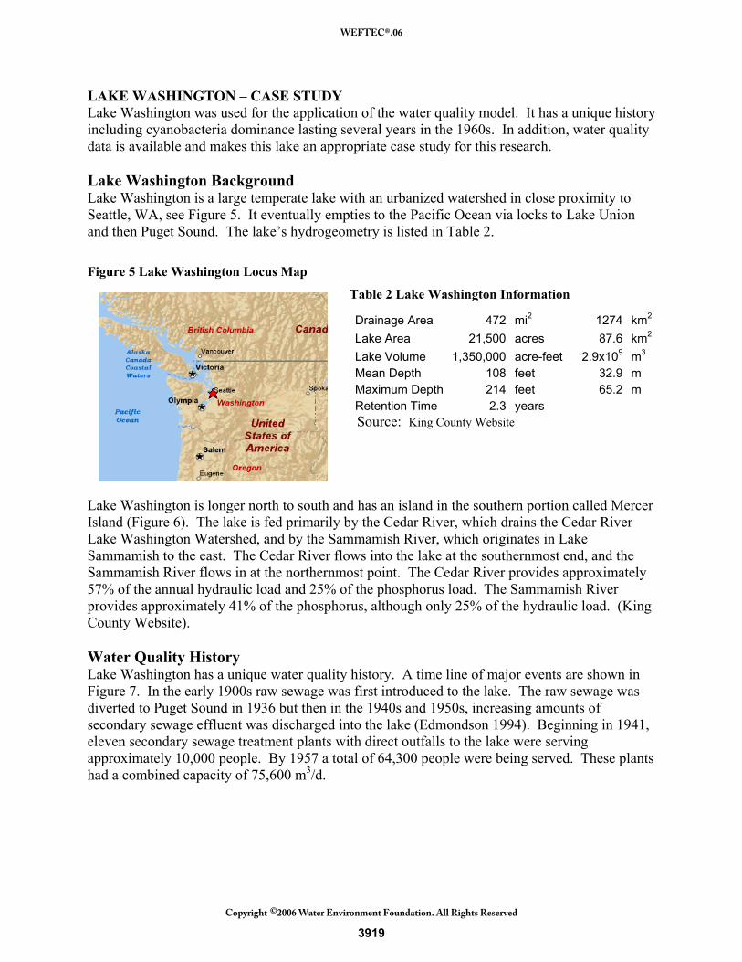
LAKE WASHINGTON – CASE STUDY Lake Washington was used for the application of the water quality model. It has a unique history including cyanobacteria dominance lasting several years in the 1960s. In addition, water quality data is available and makes this lake an appropriate case study for this research. Lake Washington Background Lake Washington is a large temperate lake with an urbanized watershed in close proximity to Seattle, WA, see Figure 5. It eventually empties to the Pacific Ocean via locks to Lake Union and then Puget Sound. The lake’s hydrogeometry is listed in Table 2. Figure 5 Lake Washington Locus Map

Table 2 Lake Washington Information

Drainage Area 472 mi2 1274 km2

Lake Area 21,500 acres 87.6 km2

Lake Volume 1,350,000 acre-feet 2.9x109 m3 Mean Depth 108 feet 32.9 m Maximum Depth 214 feet 65.2 m Retention Time 2.3 years

Source: King County Website Lake Washington is longer north to south and has an island in the southern portion called Mercer Island (Figure 6). The lake is fed primarily by the Cedar River, which drains the Cedar River Lake Washington Watershed, and by the Sammamish River, which originates in Lake Sammamish to the east. The Cedar River flows into the lake at the southernmost end, and the Sammamish River flows in at the northernmost point. The Cedar River provides approximately 57% of the annual hydraulic load and 25% of the phosphorus load. The Sammamish River provides approximately 41% of the phosphorus, although only 25% of the hydraulic load. (King County Website). Water Quality History Lake Washington has a unique water quality history. A time line of major events are shown in Figure 7. In the early 1900s raw sewage was first introduced to the lake. The raw sewage was diverted to Puget Sound in 1936 but then in the 1940s and 1950s, increasing amounts of secondary sewage effluent was discharged into the lake (Edmondson 1994). Beginning in 1941, eleven secondary sewage treatment plants with direct outfalls to the lake were serving approximately 10,000 people. By 1957 a total of 64,300 people were being served. These plants had a combined capacity of 75,600 m3/d.

3919

WEFTEC®.06


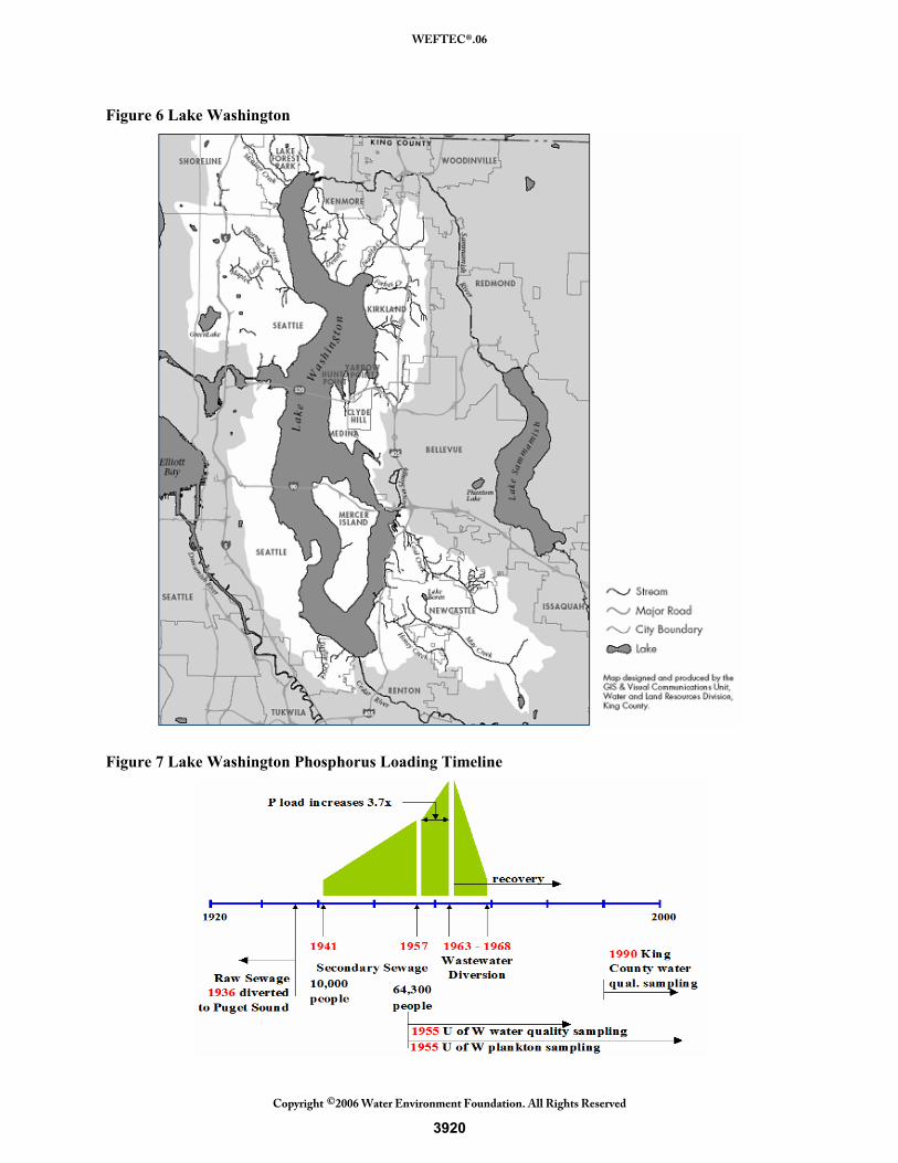
Figure 6 Lake Washington

Figure 7 Lake Washington Phosphorus Loading Timeline

3920

WEFTEC®.06


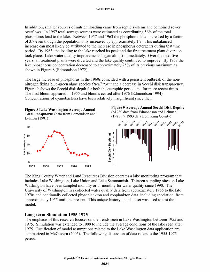
In addition, smaller sources of nutrient loading came from septic systems and combined sewer overflows. In 1957 total sewage sources were estimated as contributing 56% of the total phosphorus load to the lake. Between 1957 and 1963 the phosphorus load increased by a factor of 3.7 even though the population only increased by approximately 1.7. This unbalanced increase can most likely be attributed to the increase in phosphorus detergents during that time period. By 1963, the loading to the lake reached its peak and the first treatment plant diversion took place. Lake water quality improvements began almost immediately. Over the next five years, all treatment plants were diverted and the lake quality continued to improve. By 1968 the lake phosphorus concentration decreased to approximately 25% of its previous maximum as shown in Figure 8 (Edmondson 1972). The large increase of phosphorus in the 1960s coincided with a persistent outbreak of the non-nitrogen fixing blue-green algae species Oscillatoria and a decrease in Secchi disk transparency. Figure 9 shows the Secchi disk depth for both the eutrophic period and for more recent times. The first bloom appeared in 1955 and blooms ceased after 1976 (Edmondson 1994). Concentrations of cyanobacteria have been relatively insignificant since then. Figure 8 Lake Washington Average Annual Total Phosphorus (data from Edmondson and Lehman (1981))

Figure 9 Average Annual Secchi Disk Depths (<1980 data from Edmondson and Lehman (1981), > 1993 data from King County)

The King County Water and Land Resources Division operates a lake monitoring program that includes Lake Washington, Lake Union and Lake Sammamish. Thirteen sampling sites on Lake Washington have been sampled monthly or bi-monthly for water quality since 1990. The University of Washington has collected water quality data from approximately 1955 to the late 1970s and continually collected phytoplankton and zooplankton data, including speciation, from approximately 1955 until the present. This unique history and data set was used to test the model. Long-term Simulation 1955-1975 The emphasis of this research focuses on the trends seen in Lake Washington between 1955 and 1975. Simulation was extended to 1999 to include the average conditions of the lake seen after 1975. Justification of model assumptions related to the Lake Washington data application are summarized in McGovern (2005). The following discussion of data refers to the 1955-1975 period.

0

20

40

60

80

1955 1960 1965 1970 1975

Tota

l Pho

spho

rus

(g/

L)

0123456789

1950

1955

1960

1965

1970

1975

1980

1985

1990

1995

2000

Secc

hi D

isk

Dep

th (m

)

3921

WEFTEC®.06


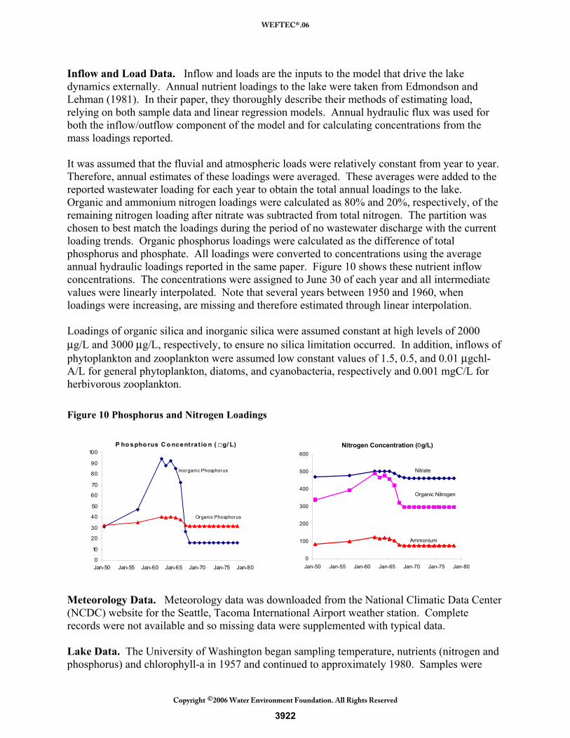
Inflow and Load Data. Inflow and loads are the inputs to the model that drive the lake dynamics externally. Annual nutrient loadings to the lake were taken from Edmondson and Lehman (1981). In their paper, they thoroughly describe their methods of estimating load, relying on both sample data and linear regression models. Annual hydraulic flux was used for both the inflow/outflow component of the model and for calculating concentrations from the mass loadings reported. It was assumed that the fluvial and atmospheric loads were relatively constant from year to year. Therefore, annual estimates of these loadings were averaged. These averages were added to the reported wastewater loading for each year to obtain the total annual loadings to the lake. Organic and ammonium nitrogen loadings were calculated as 80% and 20%, respectively, of the remaining nitrogen loading after nitrate was subtracted from total nitrogen. The partition was chosen to best match the loadings during the period of no wastewater discharge with the current loading trends. Organic phosphorus loadings were calculated as the difference of total phosphorus and phosphate. All loadings were converted to concentrations using the average annual hydraulic loadings reported in the same paper. Figure 10 shows these nutrient inflow concentrations. The concentrations were assigned to June 30 of each year and all intermediate values were linearly interpolated. Note that several years between 1950 and 1960, when loadings were increasing, are missing and therefore estimated through linear interpolation. Loadings of organic silica and inorganic silica were assumed constant at high levels of 2000 μg/L and 3000 μg/L, respectively, to ensure no silica limitation occurred. In addition, inflows of phytoplankton and zooplankton were assumed low constant values of 1.5, 0.5, and 0.01 μgchl-A/L for general phytoplankton, diatoms, and cyanobacteria, respectively and 0.001 mgC/L for herbivorous zooplankton. Figure 10 Phosphorus and Nitrogen Loadings

Meteorology Data. Meteorology data was downloaded from the National Climatic Data Center (NCDC) website for the Seattle, Tacoma International Airport weather station. Complete records were not available and so missing data were supplemented with typical data. Lake Data. The University of Washington began sampling temperature, nutrients (nitrogen and phosphorus) and chlorophyll-a in 1957 and continued to approximately 1980. Samples were

P ho spho rus C o ncentrat io n ( g/ L)

0

10

20

30

40

50

60

70

80

90

100

Jan-50 Jan-55 Jan-60 Jan-65 Jan-70 Jan-75 Jan-80

Inorganic Phosphorus

Organic Phosphorus

Nitrogen Concentration (0g/L)

0

100

200

300

400

500

600

Jan-50 Jan-55 Jan-60 Jan-65 Jan-70 Jan-75 Jan-80

Nitrate

Organic Nitrogen

Ammonium

3922

WEFTEC®.06


taken approximately bi-weekly or monthly and often excluded winter months. The measurements of interest include temperature and concentrations of ammonium nitrogen, nitrate nitrogen, dissolved phosphorus (compared with inorganic phosphorus model output), total phosphorus, and chlorophyll-a. Silica and organic nutrient measurements were not available. Sampling for phytoplankton biovolumes and zooplankton counts began in 1955 and continues today. Phytoplankton biovolumes per milliliter are reported for each species present, representing the epilimnion. As in the model, the phytoplankton measurements were grouped into diatoms, cyanobacteria, and all other species. The predominant cyanobacteria species, Oscillatoria, is not a nitrogen-fixing species and so the cyanobacteria were not divided further into nitrogen fixing and non-fixing groups. The biovolumes were converted to chlorophyll-a concentrations by assuming that biovolume proportions by group were the same as chlorophyll-a proportions. Therefore, the measured chlorophyll-a concentration for a given sampling date was divided among the groups using the biovolume proportions by group for that same date. This conversion assumes that both the biovolumes and chlorophyll-a content of species in all groups is the same and constant. These assumptions are known to be untrue, but on average best represent the make-up of phytoplankton in the lake. Zooplankton counts were converted to carbon concentration equivalents by using regression equations relating their length to carbon content. The University of Washington measured zooplankton lengths for some of the main species on select sampling dates. Averages of these lengths were applied to the appropriate species. An average of all measured lengths was applied to those species that were not measured. Finally, relationships for Daphnia, Bythotrephes and Leptodora between length and carbon content from Manca and Comoli (1999) were used to calculate zooplankton concentrations in carbon units.

3923

WEFTEC®.06


RESULTS Calibration of the values listed in Table 3 was done by trial and error. Results were based on visual inspection of the phytoplankton and nutrient results against the data, although the goal of the model was to best simulate cyanobacteria. Initial conditions used to begin the model simulation were approximated using the sampling data when available. To aid in calibration, the nutrient limitation factors for each phytoplankton group (φN) were output for each time step. As mentioned, the zooplankton data includes all species of zooplankton counted for a given sampling date. The sampling nets and depths were not consistent between sampling dates and therefore measurements were expected to contain much variability. In addition, zooplankton species were not designated between the herbivore and carnivore groups. Therefore, the zooplankton model output was compared with the data as only a gross check. The rate coefficients and parameters that produced the phytoplankton best calibration are shown in Table 3. The successful phytoplankton dynamics include the following:

low growth rate for cyanobacteria small temperature range with low optimal temperature for diatoms high phosphorus half saturation constant for cyanobacteria low nitrogen half saturation constant for cyanobacteria and general phytoplankton no settling or grazing losses for cyanobacteria lower settling and grazing losses for general phytoplankton (compared to diatoms)

In general the model was capable of simulating nutrients more accurately using different rate coefficients, but only at the expense of the phytoplankton results. When calibration was focused on only the quality of the nutrient results, more accurate results were obtained, but phytoplankton simulations were not as accurate. The analysis of the model was divided into long-term and short-term trend comparison. Annual averaged data was compared to annual average model output to examine overall long-term trends. Short-term, seasonal trend comparison used model output on a daily time-step compared to discrete measurement data for both eutrophic and average periods. Long-term Results and Analysis Phytoplankton and temperature data was available from 1955 until 2000 and was used to run a continuous long-term simulation. Average loadings were used to fill in the years between 1975 and 1995. As mentioned, detailed data was available for 1995-2000 and was used in this long-term simulation. The long-term simulation compares annual average model output with measurement data averaged annually. Chlorophyll-a and phytoplankton group concentrations were only averaged during the growing season from April to September.

3924

WEFTEC®.06


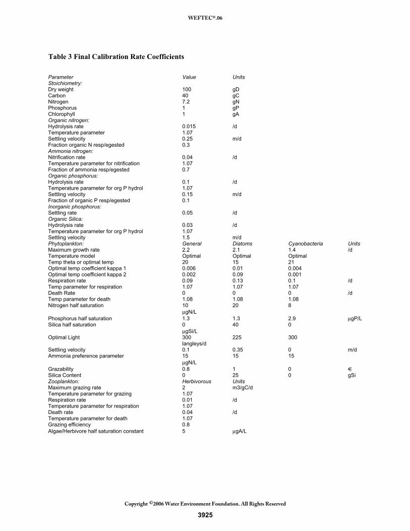
Table 3 Final Calibration Rate Coefficients

Parameter Value Units Stoichiometry: Dry weight 100 gD Carbon 40 gC Nitrogen 7.2 gN Phosphorus 1 gP Chlorophyll 1 gA Organic nitrogen: Hydrolysis rate 0.015 /d Temperature parameter 1.07 Settling velocity 0.25 m/d Fraction organic N resp/egested 0.3 Ammonia nitrogen: Nitrification rate 0.04 /d Temperature parameter for nitrification 1.07 Fraction of ammonia resp/egested 0.7 Organic phosphorus: Hydrolysis rate 0.1 /d Temperature parameter for org P hydrol 1.07 Settling velocity 0.15 m/d Fraction of organic P resp/egested 0.1 Inorganic phosphorus: Settling rate 0.05 /d Organic Silica: Hydrolysis rate 0.03 /d Temperature parameter for org P hydrol 1.07 Settling velocity 1.5 m/d Phytoplankton: General Diatoms Cyanobacteria Units Maximum growth rate 2.2 2.1 1.4 /d Temperature model Optimal Optimal Optimal Temp theta or optimal temp 20 15 21 Optimal temp coefficient kappa 1 0.006 0.01 0.004 Optimal temp coefficient kappa 2 0.002 0.09 0.001 Respiration rate 0.09 0.13 0.1 /d Temp parameter for respiration 1.07 1.07 1.07 Death Rate 0 0 0 /d Temp parameter for death 1.08 1.08 1.08 Nitrogen half saturation 10 20 8 μgN/L Phosphorus half saturation 1.3 1.3 2.9 μgP/L Silica half saturation 0 40 0 μgSi/L Optimal Light 300 225 300 langleys/d Settling velocity 0.1 0.35 0 m/d Ammonia preference parameter 15 15 15 μgN/L Grazability 0.8 1 0 € Silica Content 0 25 0 gSi Zooplankton: Herbivorous Units Maximum grazing rate 2 m3/gC/d Temperature parameter for grazing 1.07 Respiration rate 0.01 /d Temperature parameter for respiration 1.07 Death rate 0.04 /d Temperature parameter for death 1.07 Grazing efficiency 0.8 Algae/Herbivore half saturation constant 5 μgA/L

3925

WEFTEC®.06


Nitrogen. Figure 11 shows the ammonium and nitrate results. Except for 1964 and 1966 epilimnion concentrations, the model consistently over predicts ammonium levels in the lake. No organic nitrogen data was available to assist in calibration of the partition between organic nitrogen and ammonium from plankton respiration or the hydrolysis rate converting organic nitrogen to ammonium. Figure 11 Long-term Nitrogen Results

A mmo nium

0

10

20

30

40

50

60

1955 1960 1965 1970 1975 1980 1985 1990 1995 2000

Epi M odel

Hypo M odel

Epi Data

Hypo Data

Nitrate

0

100

200

300

400

500

1955 1960 1965 1970 1975 1980 1985 1990 1995 2000

ug/L

The model correctly simulates the increase of nitrate nitrogen during the loading period, but does not predict the highest concentrations measured in the mid 1960s. In addition, the model reports increasing nitrate concentrations after loadings cease and the lake is phosphorus limited. The model simulates a decrease in phytoplankton use of nitrogen during this period and therefore nitrate builds up in the system. The data instead show a decrease in nitrate. This discrepancy could be attributed to poorly estimated loads or other dynamics not represented in the model. When detailed loads are used in the 1995-2000 period, the model is able to simulate nitrate better. Phosphorus. Phosphorus long-term results are shown in Figure 12. The inorganic phosphorus model results follow the trend shown in the data of increasing values during the wastewater discharge and decreasing after diversions took place. Epilimnion model results generally match well despite high values in the 1960s. The data show that epilimnion and hypolimnion concentrations are close except during the wastewater loading period. The model shows the difference between epilimnion and hypolimnion concentrations to be relatively consistent throughout the entire simulation. This difference could be attributed to phytoplankton luxury uptake, which is not simulated in this model. During that period, phosphorus concentrations were high and the phytoplankton’s uptake rate of phosphorus might have been higher, to store

3926

WEFTEC®.06


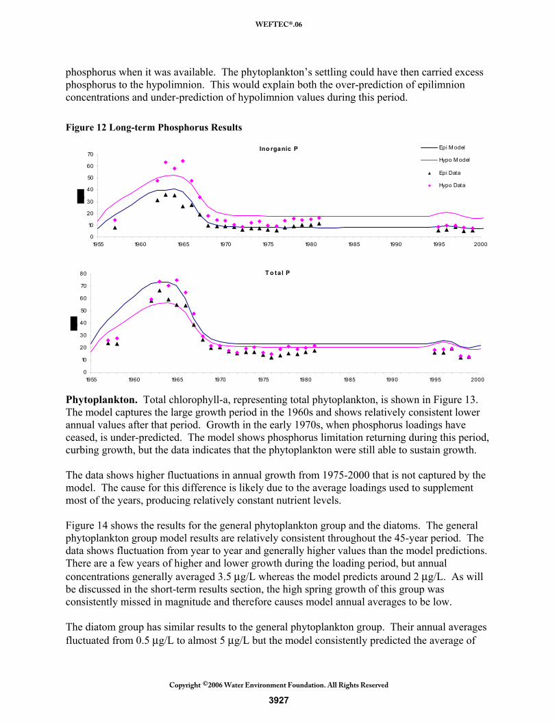
phosphorus when it was available. The phytoplankton’s settling could have then carried excess phosphorus to the hypolimnion. This would explain both the over-prediction of epilimnion concentrations and under-prediction of hypolimnion values during this period. Figure 12 Long-term Phosphorus Results

Ino rganic P

0

10

20

30

40

50

60

70

1955 1960 1965 1970 1975 1980 1985 1990 1995 2000

Epi M odel

Hypo M odel

Epi Data

Hypo Data

T o ta l P

0

10

20

30

40

50

60

70

80

1955 1960 1965 1970 1975 1980 1985 1990 1995 2000

Phytoplankton. Total chlorophyll-a, representing total phytoplankton, is shown in Figure 13. The model captures the large growth period in the 1960s and shows relatively consistent lower annual values after that period. Growth in the early 1970s, when phosphorus loadings have ceased, is under-predicted. The model shows phosphorus limitation returning during this period, curbing growth, but the data indicates that the phytoplankton were still able to sustain growth. The data shows higher fluctuations in annual growth from 1975-2000 that is not captured by the model. The cause for this difference is likely due to the average loadings used to supplement most of the years, producing relatively constant nutrient levels. Figure 14 shows the results for the general phytoplankton group and the diatoms. The general phytoplankton group model results are relatively consistent throughout the 45-year period. The data shows fluctuation from year to year and generally higher values than the model predictions. There are a few years of higher and lower growth during the loading period, but annual concentrations generally averaged 3.5 μg/L whereas the model predicts around 2 μg/L. As will be discussed in the short-term results section, the high spring growth of this group was consistently missed in magnitude and therefore causes model annual averages to be low. The diatom group has similar results to the general phytoplankton group. Their annual averages fluctuated from 0.5 μg/L to almost 5 μg/L but the model consistently predicted the average of

3927

WEFTEC®.06


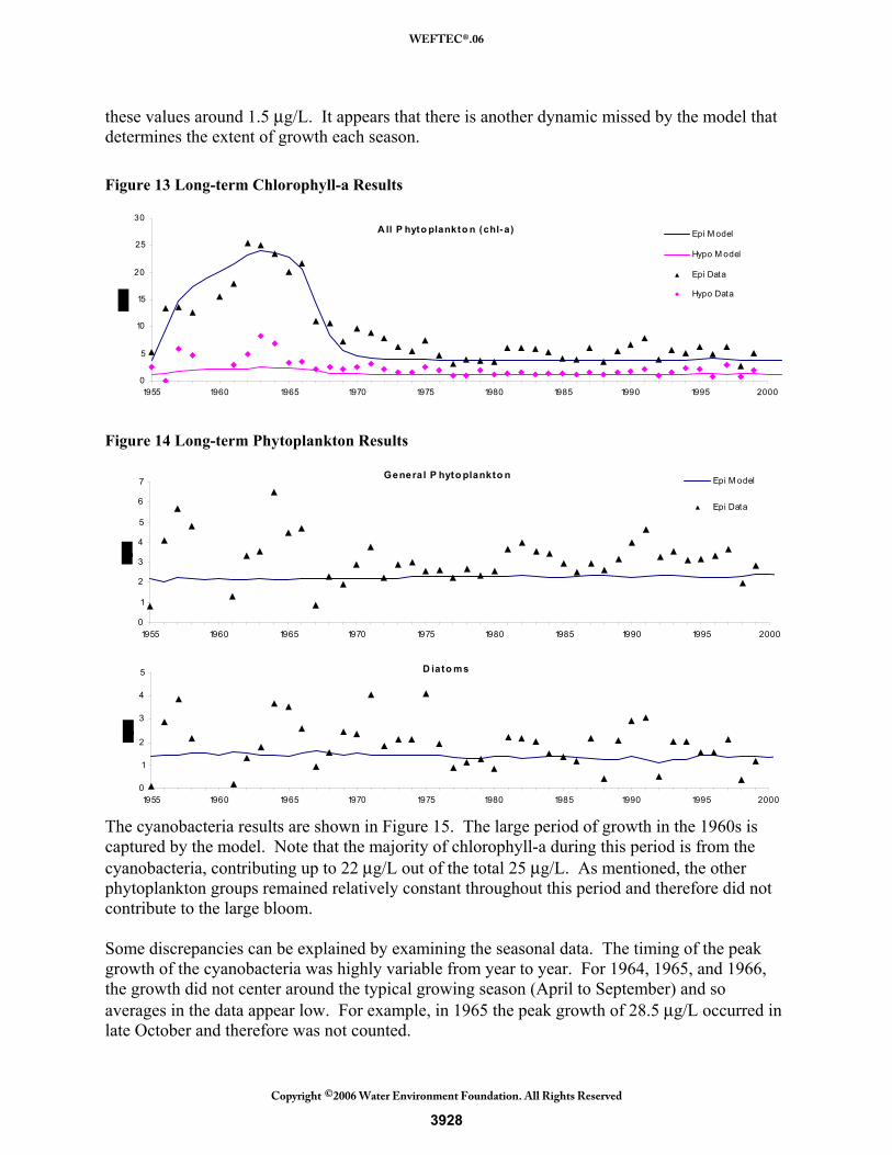
these values around 1.5 μg/L. It appears that there is another dynamic missed by the model that determines the extent of growth each season. Figure 13 Long-term Chlorophyll-a Results

A ll P hyto plankto n (chl-a)

0

5

10

15

20

25

30

1955 1960 1965 1970 1975 1980 1985 1990 1995 2000

Epi M odel

Hypo M odel

Epi Data

Hypo Data

Figure 14 Long-term Phytoplankton Results

General P hyto plankto n

0

1

2

3

4

5

6

7

1955 1960 1965 1970 1975 1980 1985 1990 1995 2000

Epi M odel

Epi Data

D iato ms

0

1

2

3

4

5

1955 1960 1965 1970 1975 1980 1985 1990 1995 2000

The cyanobacteria results are shown in Figure 15. The large period of growth in the 1960s is captured by the model. Note that the majority of chlorophyll-a during this period is from the cyanobacteria, contributing up to 22 μg/L out of the total 25 μg/L. As mentioned, the other phytoplankton groups remained relatively constant throughout this period and therefore did not contribute to the large bloom. Some discrepancies can be explained by examining the seasonal data. The timing of the peak growth of the cyanobacteria was highly variable from year to year. For 1964, 1965, and 1966, the growth did not center around the typical growing season (April to September) and so averages in the data appear low. For example, in 1965 the peak growth of 28.5 μg/L occurred in late October and therefore was not counted.

3928

WEFTEC®.06


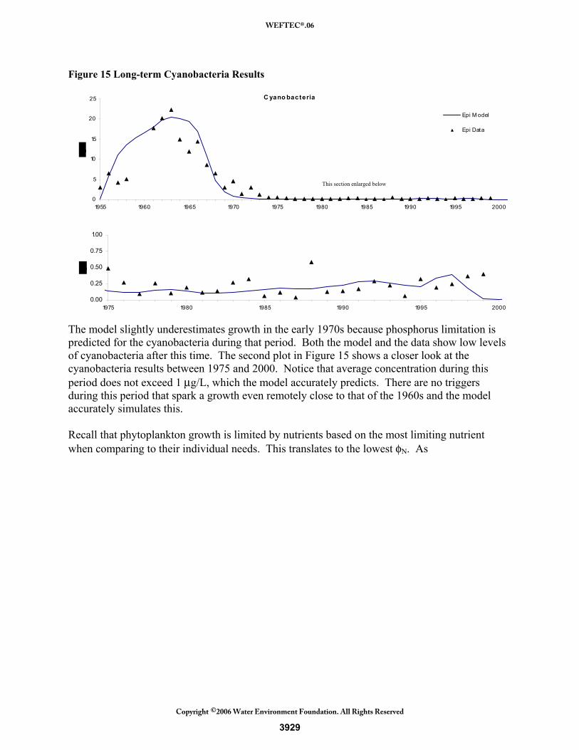
Figure 15 Long-term Cyanobacteria Results

C yano bacteria

0

5

10

15

20

25

1955 1960 1965 1970 1975 1980 1985 1990 1995 2000

Epi M odel

Epi Data

0.00

0.25

0.50

0.75

1.00

1975 1980 1985 1990 1995 2000

The model slightly underestimates growth in the early 1970s because phosphorus limitation is predicted for the cyanobacteria during that period. Both the model and the data show low levels of cyanobacteria after this time. The second plot in Figure 15 shows a closer look at the cyanobacteria results between 1975 and 2000. Notice that average concentration during this period does not exceed 1 μg/L, which the model accurately predicts. There are no triggers during this period that spark a growth even remotely close to that of the 1960s and the model accurately simulates this. Recall that phytoplankton growth is limited by nutrients based on the most limiting nutrient when comparing to their individual needs. This translates to the lowest φN. As

This section enlarged below

3929

WEFTEC®.06


Figure 16 shows, nitrogen quickly becomes the limiting nutrient during the 1960s when phosphorus loadings were high. In the 1970s when wastewater loadings were no longer contributing large amounts of nutrients, the lake flushed out excess phosphorus and once again, phosphorus became the limiting nutrient. Comparing the individual groups, cyanobacteria has a lower nitrogen half-saturation constant and therefore is less nitrogen limited during the 1960s than the other groups. This trait gives them the advantage, along with no settling and grazing losses, and allows them to flourish during this time. When phosphorus levels decrease, cyanobacteria become phosphorus limited to a great extent because of their high phosphorus needs (high phosphorus half-saturation constant). The other groups are also phosphorus limited, but not as severely as the cyanobacteria. Notice that both the diatoms and the general phytoplankton group have relatively consistent nutrient limitation throughout the entire simulation. The limiting nutrient does change from nitrogen to phosphorus, but their overall nutrient limitation remains the same and therefore produces consistent growth throughout the period.

3930

WEFTEC®.06


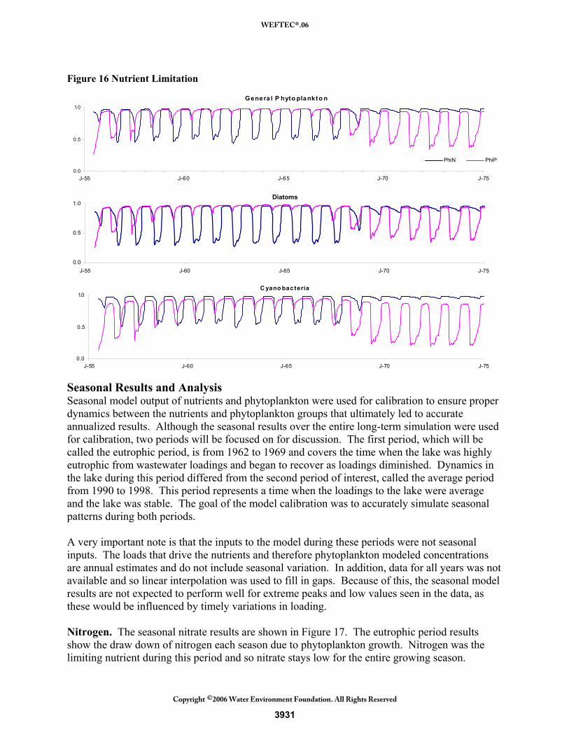
Figure 16 Nutrient Limitation

Genera l P hyto pla nkto n

0.0

0.5

1.0

J-55 J-60 J-65 J-70 J-75

PhiN PhiP

Diatoms

0.0

0.5

1.0

J-55 J-60 J-65 J-70 J-75 C yano bacteria

0.0

0.5

1.0

J-55 J-60 J-65 J-70 J-75

Seasonal Results and Analysis Seasonal model output of nutrients and phytoplankton were used for calibration to ensure proper dynamics between the nutrients and phytoplankton groups that ultimately led to accurate annualized results. Although the seasonal results over the entire long-term simulation were used for calibration, two periods will be focused on for discussion. The first period, which will be called the eutrophic period, is from 1962 to 1969 and covers the time when the lake was highly eutrophic from wastewater loadings and began to recover as loadings diminished. Dynamics in the lake during this period differed from the second period of interest, called the average period from 1990 to 1998. This period represents a time when the loadings to the lake were average and the lake was stable. The goal of the model calibration was to accurately simulate seasonal patterns during both periods. A very important note is that the inputs to the model during these periods were not seasonal inputs. The loads that drive the nutrients and therefore phytoplankton modeled concentrations are annual estimates and do not include seasonal variation. In addition, data for all years was not available and so linear interpolation was used to fill in gaps. Because of this, the seasonal model results are not expected to perform well for extreme peaks and low values seen in the data, as these would be influenced by timely variations in loading. Nitrogen. The seasonal nitrate results are shown in Figure 17. The eutrophic period results show the draw down of nitrogen each season due to phytoplankton growth. Nitrogen was the limiting nutrient during this period and so nitrate stays low for the entire growing season.

3931

WEFTEC®.06


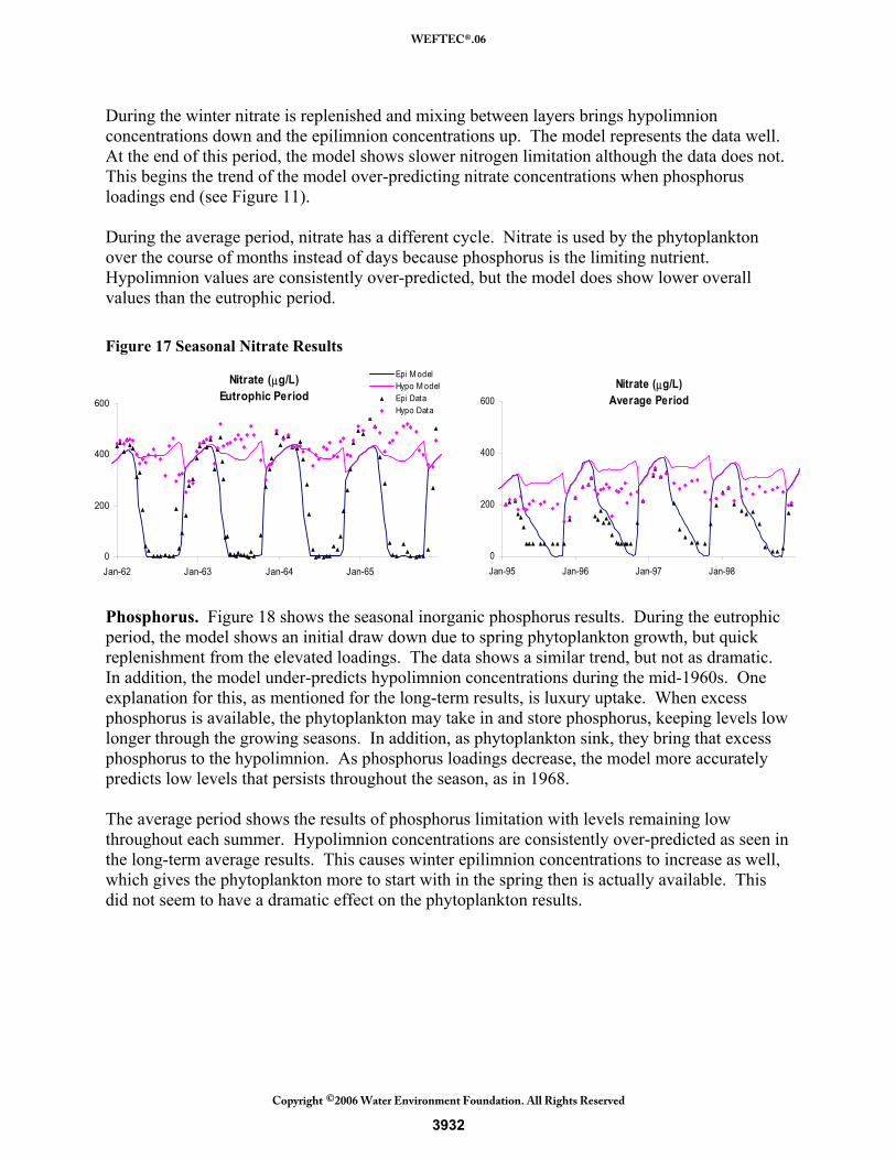
During the winter nitrate is replenished and mixing between layers brings hypolimnion concentrations down and the epilimnion concentrations up. The model represents the data well. At the end of this period, the model shows slower nitrogen limitation although the data does not. This begins the trend of the model over-predicting nitrate concentrations when phosphorus loadings end (see Figure 11). During the average period, nitrate has a different cycle. Nitrate is used by the phytoplankton over the course of months instead of days because phosphorus is the limiting nutrient. Hypolimnion values are consistently over-predicted, but the model does show lower overall values than the eutrophic period. Figure 17 Seasonal Nitrate Results

Phosphorus. Figure 18 shows the seasonal inorganic phosphorus results. During the eutrophic period, the model shows an initial draw down due to spring phytoplankton growth, but quick replenishment from the elevated loadings. The data shows a similar trend, but not as dramatic. In addition, the model under-predicts hypolimnion concentrations during the mid-1960s. One explanation for this, as mentioned for the long-term results, is luxury uptake. When excess phosphorus is available, the phytoplankton may take in and store phosphorus, keeping levels low longer through the growing seasons. In addition, as phytoplankton sink, they bring that excess phosphorus to the hypolimnion. As phosphorus loadings decrease, the model more accurately predicts low levels that persists throughout the season, as in 1968. The average period shows the results of phosphorus limitation with levels remaining low throughout each summer. Hypolimnion concentrations are consistently over-predicted as seen in the long-term average results. This causes winter epilimnion concentrations to increase as well, which gives the phytoplankton more to start with in the spring then is actually available. This did not seem to have a dramatic effect on the phytoplankton results.

Nitrate (μg/L)Eutrophic Period

0

200

400

600

Jan-62 Jan-63 Jan-64 Jan-65

Epi M odelHypo M odelEpi DataHypo Data

Nitrate (μg/L)Average Period

0

200

400

600


3932

WEFTEC®.06


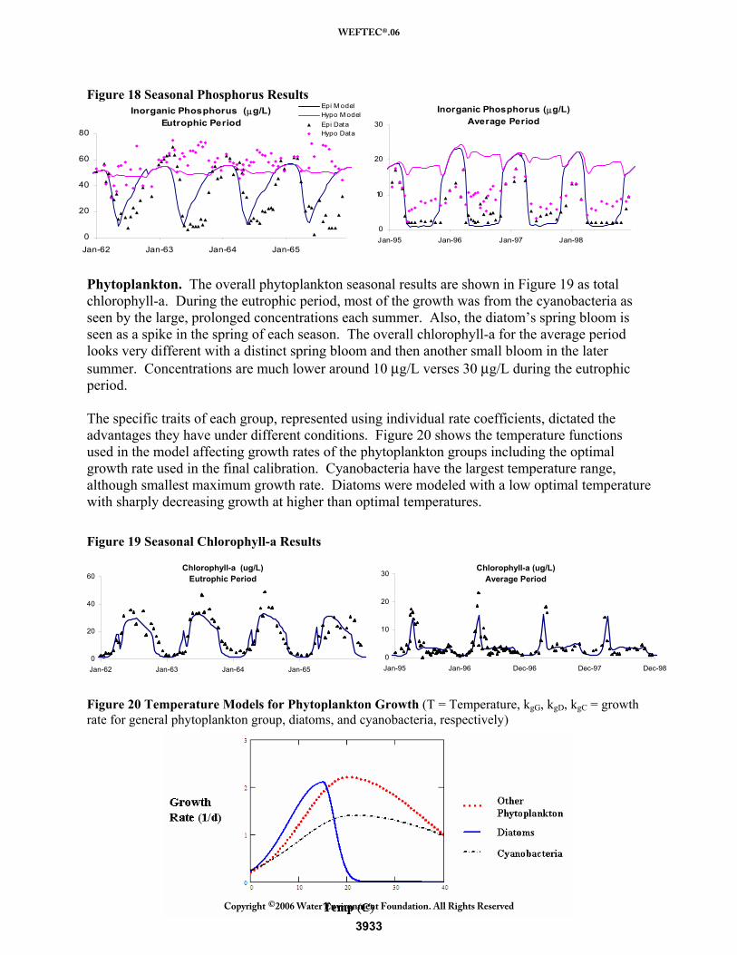
Figure 18 Seasonal Phosphorus Results

Phytoplankton. The overall phytoplankton seasonal results are shown in Figure 19 as total chlorophyll-a. During the eutrophic period, most of the growth was from the cyanobacteria as seen by the large, prolonged concentrations each summer. Also, the diatom’s spring bloom is seen as a spike in the spring of each season. The overall chlorophyll-a for the average period looks very different with a distinct spring bloom and then another small bloom in the later summer. Concentrations are much lower around 10 μg/L verses 30 μg/L during the eutrophic period. The specific traits of each group, represented using individual rate coefficients, dictated the advantages they have under different conditions. Figure 20 shows the temperature functions used in the model affecting growth rates of the phytoplankton groups including the optimal growth rate used in the final calibration. Cyanobacteria have the largest temperature range, although smallest maximum growth rate. Diatoms were modeled with a low optimal temperature with sharply decreasing growth at higher than optimal temperatures. Figure 19 Seasonal Chlorophyll-a Results

Figure 20 Temperature Models for Phytoplankton Growth (T = Temperature, kgG, kgD, kgC = growth rate for general phytoplankton group, diatoms, and cyanobacteria, respectively)

Chlorophyll-a (ug/L)Average Period

0

10

20

30

Jan-95 Jan-96 Dec-96 Dec-97 Dec-98

Chlorophyll-a (ug/L) Eutrophic Period

0

20

40

60


Inorganic Phosphorus (μg/L)

Average Period

0

10

20

30


Inorganic Phosphorus (μg/L)Eutrophic Period

0

20

40

60

80


Epi M odelHypo M odelEpi DataHypo Data

3933

WEFTEC®.06


Figure 21 shows the seasonal results of the general phytoplankton group. The eutrophic period begins with two years of spring blooms and another low growth period during the later summer. The following years show a different trend of high growth during only the late summer. This difference could be the result of different speciation of this group during the period of maximum phosphorus. The model lumps all remaining species in this group and therefore would not represent this. The average period again shows the trend of a large spring bloom and a smaller summer bloom, which the model is able to capture. One reason for the under-estimation of the spring peaks is from the excess chlorophyll-a that phytoplankton produce during large growth spurts which is not captured by the model’s fixed stoichiometry. In addition, the conversion of biomass assumes constant chlorophyll content and consistent chlorophyll content between all phytoplankton species. The summer bloom is represented well by the model. The diatoms have relatively consistent growth patterns both in the eutrophic period and in the average period, as shown by Figure 22. They repeatedly have a large spring bloom that quickly is eliminated due to their high settling velocity and grazing pressure. The temperature limitation prevents them from growing later in the season. The diatoms’ early season growth gave them access to consistently larger concentrations of winter nutrients. As shown in

3934

WEFTEC®.06


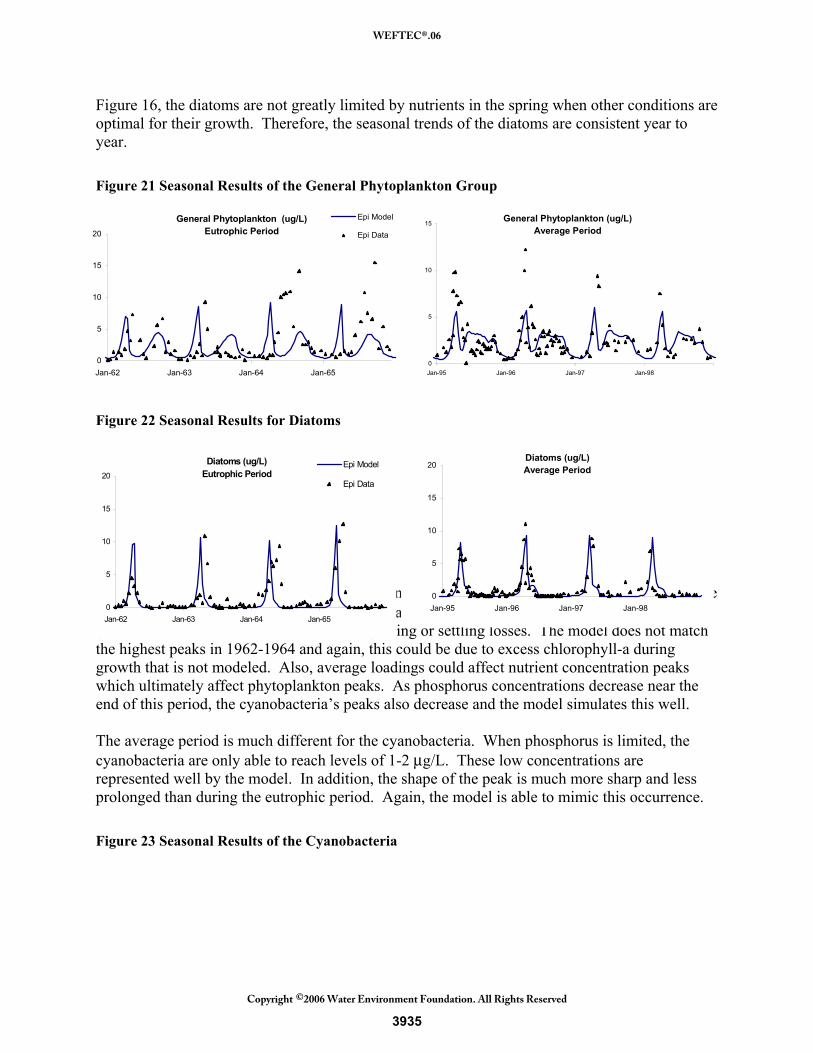
Figure 16, the diatoms are not greatly limited by nutrients in the spring when other conditions are optimal for their growth. Therefore, the seasonal trends of the diatoms are consistent year to year. Figure 21 Seasonal Results of the General Phytoplankton Group

Figure 22 Seasonal Results for Diatoms

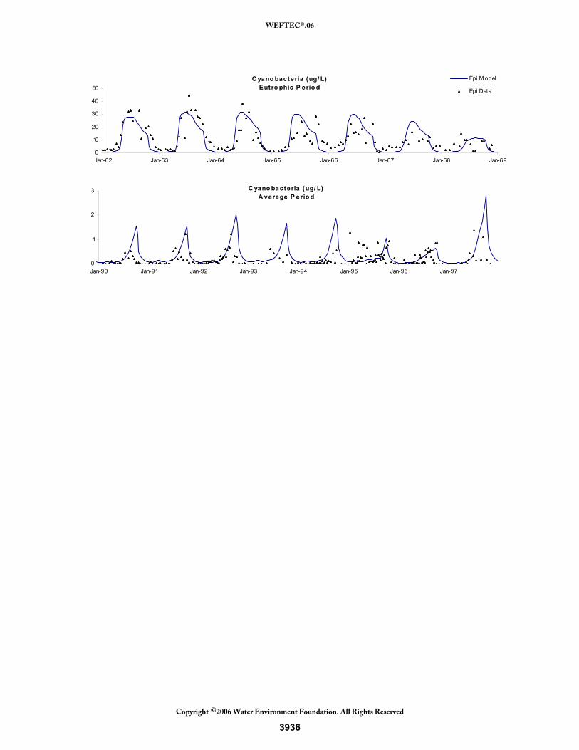
The cyanobacteria seasonal results are shown in Figure 23. The eutrophic period shows the large growth (over 30 μg/L) occurring for several years. The model represents this well, showing growth that lasts several months due to no grazing or settling losses. The model does not match the highest peaks in 1962-1964 and again, this could be due to excess chlorophyll-a during growth that is not modeled. Also, average loadings could affect nutrient concentration peaks which ultimately affect phytoplankton peaks. As phosphorus concentrations decrease near the end of this period, the cyanobacteria’s peaks also decrease and the model simulates this well. The average period is much different for the cyanobacteria. When phosphorus is limited, the cyanobacteria are only able to reach levels of 1-2 μg/L. These low concentrations are represented well by the model. In addition, the shape of the peak is much more sharp and less prolonged than during the eutrophic period. Again, the model is able to mimic this occurrence. Figure 23 Seasonal Results of the Cyanobacteria

Diatoms (ug/L)Average Period

0

5

10

15

20


Diatoms (ug/L)Eutrophic Period

0

5

10

15

20


Epi Model

Epi Data

General Phytoplankton (ug/L)Average Period

0

5

10

15


General Phytoplankton (ug/L)Eutrophic Period

0

5

10

15

20


Epi Model

Epi Data

3935

WEFTEC®.06


C yano bacteria (ug/ L)Eutro phic P erio d

0

10

20

30

40

50

Jan-62 Jan-63 Jan-64 Jan-65 Jan-66 Jan-67 Jan-68 Jan-69

Epi M odel

Epi Data

C yano bacteria (ug/ L)

A verage P erio d

0

1

2

3

Jan-90 Jan-91 Jan-92 Jan-93 Jan-94 Jan-95 Jan-96 Jan-97

3936

WEFTEC®.06


CONCLUSIONS Overall, the results show that long-term cyanobacteria trends of growth can be simulated using average yearly loadings. This is true for Lake Washington but might not be true for lakes with shorter residence times. Although not all seasonal peaks were matched, periods of growth for all of the phytoplankton groups are modeled well. Standard water quality variables were used and only rate coefficients were needed to obtain successful separate phytoplankton group results. No complicated modeling was needed to differentiate cyanobacteria from the other groups. Instead, nutrient concentrations were the main driving factors to the phytoplankton growth and cyanobacteria dominance. The process of calibration emphasized the competitiveness of the phytoplankton groups for nutrients. The success or failure of each group affected the other groups. By manipulating the “traits” of each group, represented by their individual rate coefficients and parameters, each group was simulated well. It was not only essential to accurately represent the cyanobacteria, as their success rests on their competitive advantages over the other groups. All groups were needed to simulate the correct phytoplankton dynamics. It was the differences of the cyanobacteria’s growth (through temperature and nutrients) and losses that produced successful long-term and seasonal simulations. The results of this model give insight to some of cyanobacteria’s characteristics. Influential Characteristics Several ideas about cyanobacteria from the literature (summarized in Section 2) worked together in the model to give successful seasonal results. First, cyanobacteria were not grazed which is consistent with the reported experiments in Section 2. Because the cyanobacteria were not suppressed by grazing pressure in the model, they were allowed to grow at high levels for long periods, if other conditions were favorable. This competitive advantage allowed their numbers to multiply while the other groups were lost to grazing. To represent the cyanobacteria’s ability to be buoyant, they did not settle in the model. Again, by not being lost in this way, the cyanobacteria are allowed more opportunity for light and nutrients by remaining in the epilimnion, giving them a competitive advantage in the model. In addition, the low optimal growth rate used in the model worked well to predict cyanobacteria growth only when all conditions were favorable for a long enough period of time. The combination of having a low optimal growth rate and not having settling or grazing losses for cyanobacteria simulated the broad growth peaks seen in the data during the eutrophic period. The results indicate that these characteristics are important for the cyanobacteria’s growth and survival. Cyanobacteria’s low N:P ratio needs were discussed in the literature both in general and specifically in regards to nitrogen-fixing species. In the case of Lake Washington, a non-nitrogen fixer was the dominant species, but the low N:P ratio still proved advantageous for the cyanobacteria. Giving the cyanobacteria a low nitrogen half-saturation constant and a high phosphorus half-saturation constant in the model caused them to grow and dominate during the large phosphorus loading when N:P ratios were low. When loadings were reduced and the lake

3937

WEFTEC®.06


became primarily phosphorus limited again (N:P ratio higher), the cyanobacteria remain at low levels. The relative ratio of nutrients was important in determining the growth-limiting nutrient for each phytoplankton group. The model shows that at N:P concentration ratios below about 8 and above 3, the cyanobacteria have an advantage. In this range, the general phytoplankton group and the diatoms become nitrogen limited, while cyanobacteria were not. Knowing the turning point of nutrient limitation is important for making the most effective decisions for eutrophication management. Managers can focus on decreasing inputs of only the limiting nutrient to levels at which phytoplankton growth will be prohibited. Characteristics Not Represented in the Model Several theories of dominance dealing with cyanobacteria characteristics were omitted from this model for simplification. Although there have been extensive experiments and models showing the vertical movement patterns of cyanobacteria, this was not simulated in the model. Vertical movement allows them access to light and nutrients throughout the water column. The model still performed well giving them the same light and nutrient exposure as the other phytoplankton groups. The epilimnion is assumed to be a completely mixed layer with equal amounts of nutrients and average light conditions for all phytoplankton residing there. This assumption may be accurate enough to downplay any advantage the cyanobacteria might have by vertical movement. Cyanobacteria have been shown to withstand high pH conditions and therefore have an advantage over other groups. The pH of Lake Washington was not simulated and pH data was not available for comparison. The exclusion of this parameter shows that it is not a crucial factor for predicting growth and dominance, at least for lakes with moderate pH such as Lake Washington. Trace elements were also not simulated in this model, but have been speculated as triggers for cyanobacteria. Elements such as iron, manganese, cobalt, and copper (Paerl et al. 2001) are necessary for growth, although they show no indication of being limited in Lake Washington. Potentially trace elements in other water systems could have a large impact on cyanobacteria growth. Including these theories in the model might help to capture more of the intricate fluctuations of both cyanobacteria and their interactions with the nutrients and other phytoplankton groups. To be thorough, each condition or characteristic should be looked at to determine significance. The results of this work show that cyanobacteria, or at least Oscillatoria, can be simulated using phosphorus, nitrogen, and phytoplankton group dynamics. No further complicated dynamics are needed if general results and trends are desired. Cyanobacteria are mainly triggered by nutrient dynamics and use their competitive advantages of minimal settling and grazing losses to account for slow growth. Other characteristics of either cyanobacteria or the water body are not major influences on growth and dominance.

3938

WEFTEC®.06


REFERENCES Arhonditsis, G.B., and Brett, M.T. 2005a. Eutrophication model for Lake Washington (USA) Part I – Model description and sensitivity analysis. Ecological Modeling. In Press Arhonditsis, G.B., and Brett, M.T. 2005b. Eutrophication model for Lake Washington (USA) Part II – model calibration and system dynamics analysis. Ecological Modeling. In Press Arhonditsis, G., Brett, M. T., Frodge, J. 2003. Environmental Control and Limnological Impacts of a Large Recurrent Spring Bloom in Lake Washington, USA. Environmental Management. 31(5):603-618. Bierman, V.J. and Dolan, D.M. 1981. Modeling of Phytoplankton-Nutrient Dynamics in Saginaw Bay, Lake Huron. J.Great lakes Res. 7(4):409-439. Canale, R.P. and Vogel, A.H. 1974. Effects of Temperature on Phytoplankton Growth. Journal of Environmental Engineering Division ASCE. 100(EE1):231-241 Canale, R.P., DePalma, L.M. and Vogel, A.H. 1976. A Plankton-Based Food Web Model for Lake Michigan. Modeling Biochemical Processes in Aquatic Ecosystems, R.P. Canale ed., Ann Arbor Science, Ann Arbor, MI Chapra, Steven C. 1997. Surface Water-Quality Modeling. McGraw-Hill Companies Inc. New York. Cerco, C.F. and Noel, M.R. 2003. Three Dimensional Eutrophication Model of Lake Washington, Prepared for King County Department of Natural Resources and Parks. Edmondson, W.T. 1966. Changes in oxygen deficit of Lake Washington. Verh. Internat. Verein. Limnol. 16:153-158. Edmondson, W.T. 1972. Nutrients and Phytoplankton in Lake Washington. Nutrients and Eutrophication: The limiting-nutrient controversy. (Ed.) G.E. Likens. American Society of Limnology and Oceanography. Lawrence (KA). 172-193 Edmondson, W. T. and Lehman, J. T. 1981. The effect of changes in the nutrient income on the condition of Lake Washington. Limnology and Oceanography. 26(1):1-29. Edmondson, W.T. 1994. Sixty Years of Lake Washington: a Curriculum Vitae. Lake and Reserv. Manage. 10(2):75-84. Edmondson, W.T. 1997. Aphanizomenon in Lake Washington. Arch. Hydrobiol./Suppl. 107(4): 409-446. Edmondson, W.T., Abella, S.E.B., and Lehman, J.T. 2003. Phytoplankton in Lake Washington: long term changes 1950-1999. Arch.Hydrobiol. 139(3):275-326. Elliott, J.A., Reynolds, C.S. and Irish, A.E. 2001. An investigation of dominance in phytoplankton using the PROTECH model. Freshwater Biology. 46:99-108. Hamilton, D.P. and Schladow, S.G. 1997. Prediction of water quality in lakes and reservoirs. Part I – Model description. Ecological Modelling. 96:91-110. Ferber, L.R., Levine, S.N., Lini, A., and Livingston, G.P. 2004. Do cyanobacteria dominate in eutrophic lakes because they fix atmospheric nitrogen? Freshwater Biology. 49:690-708. Graham, L.E. and Wilcox, L.W. 2000. Algae. Prentice-Hall, Upper Saddle River, NJ.

3939

WEFTEC®.06


Hambright, K.D., Zohary, T., Easton, J., Azoulay, B. and Fishbein, T. 2001. Effects of zooplankton grazing and nutrients on the bloom-forming, N2-fixing cyanobacterium Aphanizomenon in Lake Kinneret. Journal of Plankton Research. 23(2):165-174. Hamilton, D.P. and Schladow, S.G. 1996a. Prediction of water quality in lakes and reservoirs. Part I – Model description. Ecological Modelling. 96:91-110. Hamilton, D.P. and Schladow, S.G. 1996b. Prediction of water quality in lakes and reservoirs. Part II – Model calibration, sensitivity analysis and application. Ecological Modelling. 96:111-123. Havens, K.E., James, R.T., East, T.L., and Smith, V.H. 2002. N:P ratios, light limitation, and cyanobacterial dominance in a subtropical lake impacted by non-point source nutrient pollution. Environmental Pollution. 122:379-390. Horne, A.J., Sandusky, J.C. and Carmiggelt, C.J.W. 1979. Nitrogen Fixation in Clear Lake, California. 3. Repetitive Synoptic Sampling of the Spring Aphanizomenon Blooms. Limnology and Oceanography. 24(2):316-328. Howard, A. 1993. SCUM – Simulation of cyanobacterial underwater movement. Cabios. 9(4):413-419 Howard, A., Irish, A.E. and Reynolds, C.S. 1996. A new simulation of cyanobacterial underwater movement (SCUM’96). Journal of Plankton Research. 18(8):1375-1385. Howard, A. 1997. Computer simulation modeling of buoyant change in Microcystis. Hydrobiologia. 349:11-117. Howard, A. 2001. Modeling movement patters of the cyanobacterium Microcystis. Ecological Applications. 11(1):304-310. Howarth, R.W. and Marino, R. 1990. Mitrogen-Fixing Cyanobacteria in the Plankton of Lakes and Estuaries: A Reply to the Comment by Smith. Limnology and Oceanography. 35(8):1859-1863 Howarth, R.W., Marino, R., Lane, J. and Cole, J.J. 1988a. Nitrogen Fixation in Freshwater, Estuarine, and Marine Ecosystems. 1.Rates and Importance. Limnology and Oceanography. 33(4):669-687. Howarth, R.W., Marino, R., Lane, J. and Cole, J.J. 1988b. Nitrogen Fixation in Freshwater, Estuarine, and Marine Ecosystems. 2. Biogeochemical Controls. Limnology and Oceanography. 33(4):688-701. HydroQual, Inc. 1991. Development and Calibration of a Two Functional Algal Group Model of the Potomac Estuary. Prepared for the Metropolitan Washington Council of Governments, Washington, D.C. Infante, A. and Abella, S.E.B. 1985. Inhibition of Daphnia by Oscillatoria in Lake Washington. Limnology and Oceanography. 30(5):1046-1052. King County website: http://dnr/metrokc.gov/wlr/ Kromkamp, J.C. and Mur, L.R. 1984. Buoyant density changes in the cyanobacterium Microcystis aeruginosa due to changes in the cellular carbohydrate content. FEMS Microbiology Letters. 25:105-109.

3940

WEFTEC®.06


Lehman, J.T., Abella, S.E.B., Litt, A.H., Edmondson, W.T. 2004. Fingerprints of biocomplexity: Taxon-specific growth of phytoplankton in relation to environmental factors. Limnology and Oceanography. 49(4):1446-1456. Lehman, J.T., Botkin, D.B. and Likens, G.E. 1975. The Assumptions and Rationales of a Computer Model of Phytoplankton Population Dynamics. Limnology and Oceanography. 20(3):343-364. Lehtimaki, J., Moisander, P., Sivonen, K., and Kononen, K. 1997. Growth, Nitrogen Fixation, and Nodularin Production by Two Baltic Sea Cyanobacteria. Applied and Environmental Microbiology. 63(5):1647-1656. Lewis, W.M. and Levine, S.N. 1984. The Light Response of Nitrogen Fication in Lake Valencia, Venezuela. Limnology and Oceanography. 29(4):894-900. Lung, W.S. and Paerl, H.W. 1988. Modeling Blue-Green Algal Blooms in the Lower Neuse River. Wat. Res. 22(7):895-905. McGovern, Theresa. 2005. Lake Water Quality Model with Focus on Cyanobacteria. Tufts University. Manca, Marina and Comoli, Patrizia. 2000. Biomass estimates of fresh water zooplankton from length-carbon regression equations. Journal of Limnology. 59(1):15-18. Mugidde, R., Hecky, R.E., Hendzel, L.L. and Taylor, W.D. 2003. Pelagic Nitrogen Fixation in Lake Victoria (East Africa). Great Lakes Res. 29:76-88. Mur, L.R., Skulber, O.M. and Utkilen, H. 1999. Chapter 2. Cyanobacteria in the Environment. Toxic Cyanobacteria in Water: A guide to their public health consequences, monitoring and management. World Health Organization www.who.int/docstore/water_sanitation_health/toxiccyanobact/ Omlin, M., Peichert, P. and Forster, R. 2001. Biogeochemical model of Lake Zurich: model equations and results. Ecological Modelling. 141:77-103. Paerl, H.W., Fulton, R.S., Moisander, P.H. and Dyble, J. 2001. Harmful Freshwater Algal Blooms, With an Emphasis on Cyanobacteria. The Scientific World. 1:76-113. Paerl, H.W. 1988. Nuisance Phytoplankton Blooms in Coastal, Estuarine, and Inland Waters. Limnology and Oceanography. 33(4):823-847. Paerl, H.W., Tucker, J. and Bland, P.T. 1983. Carotenoid Enhancement and its Role in Maintaining Blue-Green Algal (Microcystis aeruginosa) Surface Blooms. Limnology and Oceanography. 28(5):847-857. Paerl, H.W. and Ustach, J.F. 1982. Blue-Green Algal Scums: An Explanation for Their Occurrence During Freshwater Blooms. Limnology and Oceanography. 27(2):212-217. PROTECH general information: www.ife.ac.uk/algalmodeling/contents/ProtechC/ProtechCPage.htm Reynolds, C.S. 1984. The ecology of freshwater phytoplankton. Cambridge University Press. Cambridge, UK. Riley, G.A. 1956. Oceanography of Long Island Sound 1952-1954. II. Physical Oceanography. Bull. Bingham. Oceanog. Collection 15. 15-16

3941

WEFTEC®.06


Robarts, R.D. and Zohary, T. 1987. 1987. Temperature effects on photosynthetic capacity, respiration, and growth rates of bloom-forming cyanobacteria. New Zealand Journal of Marine and Freshwater Research. 21:391-399. Sanudo-Wilhelmy, S.A., Kustka, A.B., Gobler, C.J., Hutchins, D.A., Yang, M., Lwiza, K., Burns, J., Capone, D.G., Raven, J.A. and Carpenter, E.J. 2001. Phosphorus limitation of nitrogen fixation by Trichodesmium in the central Atlantic Ocean. Nature. 411(6833):66-69. Shapiro, J. 1990. Current beliefs regarding dominance by blue-greens: The case for the importance of CO2 and pH. Verh. Internat. Verein. Limnol. 24:38-54. Smith, V.H. 1983. Low Nitrogen to Phosphorus Ratios Favor Dominance by Blue-Green Algae in Lake Phytoplankton. Science. 221(4661):669-671. Smith, V.H. 1990. Nitrogen, Phosphorus, and Nitrogen Fixation in Lacustrine and Estuarine Ecosystems. Limnology and Oceanography. 35(8):1852-1859. Stockner, J.G. and Shortreed, K.S. 1988. Response of Anabaena and Synechococcus to manipulation of nitrogen:phosphorus ratios in a lake fertilization experiment. Limnology and Oceanography. 33(6):1348-1361. Tetra Tech ISG, Inc. and Parametrix, Inc. 2003. Lake Washington Existing Conditions Report. King County Department of Natural Resources and Parks, Water and Land Resources Division Thomas, R.H. and Walsby, A.E. 1984. Buoyancy Regulation in a Strain of Microcystis. Journal of General Microbiology. 131:799-809. United States Environmental Protection Agency. 2004. AQUATOX (Release 2) Modeling Environmental Fate and Ecological Effects in Aquatic Ecosystems Volume 2: Technical Documentation www.epa.gov/waterscience/models/aquatox/technical/techdoc/pdf United States Environmental Protection Agency. 2000. AQUATOX for Windows A Modular Fate and Effects Model for Aquatic Ecosystems Release 1 Volume 3: Model Vailidation Reports www.epa.gov/waterscience/models/aquatox/validation/validationcov.pdf United States Environmental Protection Agency. 1985. Rates, Constants, and Kinetics Formulations in Surface Water Quality Modeling United States Geological Survey, 2004. Modeling Hydrodynamics, Temperature and Water Quality in Henry Hagg Lake, Oregon, 2000-03. Visser, P.M., Passarge, J. and Mur, L.R. 1997. Modeling vertical migration of the cyanobacterium Microcystis. Hydrobiologia. 349:99-109. Wool, Tim A., Ambrose, Robert B., Martin, James L., Comer, Edward A., US Environmental Protection Agency – Region 4 Atlanta, GA, Environmental Research Laboratory Athens, GA, USACE, Tetra Tech, Inc. 2005. Water Quality Analysis Simulation Program (WASP) Draft User’s Manual. http://www.epa.gov/athens/wwqtsc/html/wasp.html

3942

WEFTEC®.06


Documents

Lake Water Quality Model with Focus on Cyanobacteria · cyanobacteria, the physical and chemical characteristics of the environment that cause ... simulates or does not simulate each