Embed Size (px)
Citation preview

U.S. ArmyCorps of Engineers
City of AttleboroTown of North Attleboro
Lake ComoRestoration Study
ENSR InternationalJuly 2002Document Number 9000-257-100

J:\Pubs\mw97\Projects\9000257\100\all.doc July, 2002i
CONTENTS
EXECUTIVE SUMMARY.......................................................................................................................ES-1
1.0 INTRODUCTION.................................................................................................................................1-1
1.1 Overview....................................................................................................................................1-1
1.2 Site Setting ................................................................................................................................1-2
2.0 FIELD PROGRAM DESIGN AND METHODS..................................................................................2-1
2.1 Field Program Design Approach ..............................................................................................2-1
2.2 Water Quality/Hydrology Surveys.............................................................................................2-22.2.1 Dry-Weather Survey Design .........................................................................................2-22.2.2 Wet-Weather Survey Design ........................................................................................2-22.2.3 Hydrologic Data Collection Methods ............................................................................2-32.2.4 Water Quality Data Collection Methods .......................................................................2-3
2.3 Sediment Survey Design and Methods....................................................................................2-52.3.1 Sediment Survey Design...............................................................................................2-52.3.2 Pond Sediment Thickness and Bathymetry Survey Methods .....................................2-52.3.3 Sediment Quality Sampling Methods ...........................................................................2-6
2.4 Biological Survey Design and Methods....................................................................................2-62.4.1 Biological Survey Design ..............................................................................................2-62.4.2 Biological Sampling Methods for Phytoplankton Assessment ....................................2-62.4.3 Biological Sampling Methods for Aquatic Macrophyte Assessment ...........................2-7
2.5 Field Program Methods: Quality Assurance Program.............................................................2-7
3.0 FIELD PROGRAM RESULTS ...........................................................................................................3-1
3.1 Description of Study Area and Key Features...........................................................................3-13.1.1 Leak in Outlet Dam Structure........................................................................................3-23.1.2 Storm Drain Overland Flow...........................................................................................3-2
3.2 Dry-Weather Water Quality Survey Results.............................................................................3-23.2.1 Nutrient Data..................................................................................................................3-23.2.2 Bacterial Data ................................................................................................................3-33.2.3 Other Water Quality Data..............................................................................................3-4
3.3 Wet-weather Water Quality Survey Results.............................................................................3-63.3.1 Nutrient Data..................................................................................................................3-6

CONTENTS (Cont’d)
J:\Pubs\mw97\Projects\9000257\100\all.doc July, 2002ii
3.3.2 Other Water Quality Data..............................................................................................3-6
3.4 Sediment Survey Results..........................................................................................................3-73.4.1 Pond Bathymetric Data .................................................................................................3-73.4.2 Sediment Thickness Data .............................................................................................3-73.4.3 Sediment Quality Assessment......................................................................................3-8
3.5 Biological Survey Results .........................................................................................................3-93.5.1 Phytoplankton................................................................................................................3-93.5.2 Zooplankton .................................................................................................................3-103.5.3 Chlorophyll a................................................................................................................3-103.5.4 Aquatic Plant Survey ...................................................................................................3-113.5.5 Wildlife and Fish Observations ...................................................................................3-12
3.6 Summary of Field Program Results .......................................................................................3-123.6.1 Physical Observations.................................................................................................3-123.6.2 Water Quality Observations ........................................................................................3-133.6.3 Sediment and Biological Observations.......................................................................3-13
4.0 WATERSHED ASSESSMENT ..........................................................................................................4-1
4.1 Watershed Delineation and Land Use Identification ...............................................................4-1
4.2 Landuse and Historical Changes .............................................................................................4-2
4.3 Description of Public Use Areas...............................................................................................4-3
4.4 Watershed Assessment Summary...........................................................................................4-3
5.0 SCREENING LEVEL WATERSHED MODELING APPLICATION .................................................5-1
5.1 Model Setup ..............................................................................................................................5-1
5.2 Model Development ..................................................................................................................5-2
5.3 Hydrologic Simulation Results..................................................................................................5-35.3.1 Lake Como Mean Turnover Rate and Residence Time..............................................5-35.3.2 Flow Budget for Lake Como Watershed ......................................................................5-3
5.4 Water Quality Simulation Results.............................................................................................5-45.4.1 Assessment of Present Phosphorus Loads .................................................................5-45.4.2 Phosphorus Reduction Goals for the Lake Como System..........................................5-55.4.3 Model Simulation Results for Restoration Alternatives................................................5-5
5.5 Summary of Watershed Modeling Results...............................................................................5-7

CONTENTS (Cont’d)
J:\Pubs\mw97\Projects\9000257\100\all.doc July, 2002iii
6.0 MANAGEMENT GOALS AND RECOMMENDATIONS ..................................................................6-1
6.1 Observations of Existing Problems ..........................................................................................6-1
6.2 Lake Como Restoration Goals .................................................................................................6-1
6.3 Management Recommendations .............................................................................................6-26.3.1 Repair of Leaky Dam to Maintain an Appropriate Pond Water Level .........................6-26.3.2 Dredge to Reduce Excess Growth of Aquatic Vegetation...........................................6-36.3.3 Reduce Nutrient Loads to Ponds..................................................................................6-4
7.0 REFERENCES....................................................................................................................................7-1
APPENDICES
A PHOTOS OF STORM DRAINS AND OUTLET STRUCTUREB INITIAL WATERSHED-BASED POND ASSESSMENT CHECKLISTC AERIAL PHOTOS OF THE LAKE COMO WATERSHEDD DESCRIPTION OF THE SCREENING LEVEL WATERSHED MODELE LAKE COMO MANAGEMENT FEASIBILITY ASSESSMENT

J:\Pubs\mw97\Projects\9000257\100\all.doc July, 2002iv
LIST OF TABLES
Table 3-1 Water Quality Results: Dry-Weather Sampling............................................................. 3-15
Table 3-2 Water Quality Results: Wet Weather Sampling ............................................................. 3-17
Table 3-3 Phytoplankton Density of Samples Collected in the West and Main Ponds:September 7, 2000.......................................................................................................... 3-18
Table 3-4 Phytoplankton Density of Samples Collected in the West and Main Ponds:May 29, 2001................................................................................................................... 3-20
Table 3-5 Phytoplankton Density of Samples Collected in the West and Main Ponds:August 1, 2001................................................................................................................. 3-22
Table 3-6 Phytoplankton Density of Samples Collected in the West and Main Ponds:August 30, 2001 .............................................................................................................. 3-24
Table 3-7 Summary Statistics of Zooplankton: May 29, 2001 ....................................................... 3-26
Table 3-8 Summary Statistics of Zooplankton: August 1, 2001..................................................... 3-27
Table 3-9 Chlorophyll a Concentrations Measured in the Lake Como System ............................ 3-28
Table 3-10 Sediment Chemistry Results for Sediments in Lake Como .......................................... 3-29
Table 3-11 Summary of Aquatic Vegetation Investigation in Lake Como ....................................... 3-31
Table 5-1 Lake Como Hydrology: Estimated Turnover Rates and Residence Times .................... 5-9
Table 5-2 Lake Como Hydrology: Estimated Water Budget .......................................................... 5-10
Table 5-3 Lake Como Water Quality: Estimated Phosphorus Budget .......................................... 5-11

J:\Pubs\mw97\Projects\9000257\100\all.doc July, 2002v
LIST OF FIGURES
Figure 1-1 Aerial Photograph of Lake Como and Surrounding Area................................................ 1-3
Figure 1-2 Map of Lake Como with Sampling Locations Indicated................................................... 1-4
Figure 2-1 Schematic Diagram of Automated Wet-Weather Grab Sampler .................................... 2-9
Figure 2-2 Map of Lake Como with Transect Sampling Locations Indicated ................................. 2-10
Figure 3-1 Map of Lake Como with Photographs of Key Features................................................. 3-32
Figure 3-2 Lake Como Bathymetry................................................................................................... 3-33
Figure 3-3 Lake Como Sediment Thickness.................................................................................... 3-34
Figure 3-4 Lake Como Macrophyte Biovolume ............................................................................... 3-35
Figure 3-5 Lake Como Macrophyte Cover ....................................................................................... 3-36
Figure 4-1 Lake Como Watershed Delineation.................................................................................. 4-5

J:\Pubs\mw97\Projects\9000257\100\all.doc July, 2002ES-1
EXECUTIVE SUMMARY
Lake Como is a 7-acre waterbody located in the City of Attleboro and the Town of North Attleboro,Massachusetts that experiences eutrophic conditions resulting in nuisance aquatic vegetation duringthe summertime. The Lake Como Restoration Study was undertaken by Massachusetts Departmentof Environmental Management, the City of Attleboro, and the Town of North Attleboro with assistancefrom the US Army Corps of Engineers. The study included an investigation and characterization ofexisting conditions and identification of alternatives to restore the Lake. Brief summaries of the LakeComo field program, watershed modeling evaluation, and restoration recommendations are providedbelow.
Lake Como Field Program
A series of field surveys were conducted from September 2000 through June 2002 to characterizepresent conditions in Lake Como in terms of physical, hydrologic, water quality, sediment quality, andbiological characteristics. All observations obtained during the field program are consistent withcharacterization of Lake Como as a small, highly eutrophic pond system. Lake Como was observed toreceive excessive nutrient loading combined with insufficient water volume to maintain healthy waterquality conditions. The field program resulted in several key observations of present conditions in theLake Como system including the following:
• Leak in Outlet Dam – A continuous leak was identified in the main pond’s outlet dameffectively reducing the water level and storage capacity in the Lake Como system.
• Low In-Lake Dissolved Oxygen Concentrations – D.O. concentrations in the two pondswere frequently below the water quality standard of 5.0 mg/L, with measurements as low as1.0 mg/L obtained. Low D.O. concentrations are due to the presence of an excess ofaquatic vegetation in the ponds.
• Excessive In-Lake Nutrient Concentrations - Phosphorus and nitrogen concentrations inthe two ponds were observed to be excessive during field surveys and were sufficient tosupport eutrophic conditions. For example, in-lake phosphorus concentrations ranged from30 to 310 µg/L, with a mean value of 90 µg/L. Target in-lake phosphorus concentrations of16 µg/L to 31 µg/Lwere established for Lake Como based on widely accepted evaluationguidelines. Thus, ambient phosphorus concentrations were observed to be approximately 3to 5 times higher than acceptable levels indicating that nutrient levels must be dramaticallyreduced before water quality improvements may be achieved.
• Excessive Stormwater Nutrient Concentrations – Phosphorus and nitrogen concentrationsfrom the 4 storm drains were observed to be excessive during wet-weather surveys andappeared to be a major source of elevated in-lake nutrient concentrations. For example,

J:\Pubs\mw97\Projects\9000257\100\all.doc July, 2002ES-2
phosphorus stormwater concentrations ranged from 60 to 6,200 µg/L, with a mean value of1,760 µg/L.
• Sediment Nutrients – Nutrient levels in sediments were moderate to high indicating thatsediments may act as a significant source in the overall nutrient budget, depending onoxygen levels, pH, and other factors.
• Extensive Aquatic Biological Growth - Extensive growth of phytoplankton and rooted aquaticvegetation was observed during the summertime survey. The water surface was coveredwith floating macrophytes diminishing the potential for recreational uses.
Lake Como Watershed Modeling Evaluation
A screening level watershed modeling evaluation was conducted on the Lake Como system to identifysources of impairment and to support evaluation lake restoration alternatives. The watershedmodeling evaluation provided several important insights including the following:
• Watershed Phosphorus Loading Budget – The present average annual phosphorus loadwas determined to be excessive, based on comparison of a predicted load of 105 kg/yr toan acceptable load based on widely accepted estimation guidelines of 11 to 22 kg/yr. Thus,phosphorus loads to Lake Como must be reduced by approximately a factor of 5 (from 105kg/yr to, at most, 22 kg/yr) before water quality improvements may be achieved. A largeportion of the total phosphorus load, 53%, was estimated to come from storm drains.
• Evaluation of Restoration Alternatives – Restoration alternatives, featuring reduction orremoval of storm drain loads, were evaluated using the watershed model. Removal orinfiltration of storm drain flows from the system was predicted to result in 40% to 50%reductions in average annual loads of phosphorus to the ponds. Even if the additionalphosphorus added to the soil through stormwater infiltration were to accumulate, theamount of groundwater added to the lake is relatively small. Additionally, minerals in thesoil, and plants in the immediate area, will tend to keep the phosphorus from migrating farfrom the area of infiltration. Modifications that would take advantage of stormwaterinfiltration would have to be implemented along with additional modifications in order toachieve necessary water quality improvements.
Lake Como Restoration Recommendations
The water quality problems experienced by Lake Como can be resolved, but are not minor or easilyrepaired. A combination of projects conducted in-lake and in the watershed will be required to removewater quality impairment from the Lake Como system. The following 3 restoration tasks arerecommended:

J:\Pubs\mw97\Projects\9000257\100\all.doc July, 2002ES-3
1. Repair leaky dam to support increased pond volume and water level.
2. Dredge nutrient-rich pond sediments to reduce sources of excess biological growth andincrease pond volume.
3. Reduce nutrient loading to ponds through infiltration, detention, or removal of stormwatersources.
The Lake Como Restoration Study has successfully quantified present water quality and biologicalconditions in the system. The Lake restoration projects outlined above will, if implemented, result indramatic improvements to the Lake Como system and are respectfully submitted for consideration.

J:\Pubs\mw97\Projects\9000257\100\all.doc July, 20021-1
1.0 INTRODUCTION
1.1 Overview
Lake Como (PALIS #52010) is located in the City of Attleboro and the Town of North Attleboro,Massachusetts within the Ten-Mile River Watershed (Figure 1-1). Lake Como is a small urbanwaterbody comprised of two small ponds connected by a culvert. The upstream pond, known as theWest Pond, is smaller, approximately 2 acres in size, and is located in the Town North Attleboro. Thedownstream pond, known as the Main Pond, is larger, approximately 5 acres in size, and is located inthe City of Attleboro. A roadway, Como Drive, passes between the ponds and an 18-inch culvertbeneath the road connects West Pond and Main Pond. The downstream outlet of Main Pond is on theeasternmost end of the pond and consists of an overflow weir to a culvert beneath Route 1. Outletwater from Lake Como flows into the Seven-Mile River in the City of Attleboro and eventually into theTen-Mile River. Currently, many of the homes in the section of the Lake Como watershed occupied bythe Town of North Attleboro are in the process of being sewered. Therefore, the septic systems thatthese homes originally depended on will be taken offline and wastewater will be transported out of thewatershed for treatment. This process will hopefully improve the quality of the water in Lake Como byreducing nitrogen concentrations of groundwater that infiltrates into the lake. Appendix A containsphotographs of the two ponds, culverts, and storm drain structures.
Lake Como is a eutrophic water body and is shallow and extensively vegetated during thesummertime. Eutrophication is a process of nutrient accumulation and ecosystem change that occursin aquatic ecosystems. This process occurs naturally as part of a long-term transition (e.g., from laketo marsh). Eutrophication can also occur culturally whereby the process is dramatically accelerated bythe activities of man (McNaughton and Wolf, 1973). Problems associated with Lake Comoeutrophication include dense populations of algae and rooted aquatic vegetation during thesummertime. Additionally, low water levels have been observed during the summertime and have ledto large areas of exposed lake sediment with associated foul odors due to decaying vegetation.
This Lake Como Restoration Study was undertaken by Massachusetts Department of EnvironmentalManagement, the City of Attleboro, and the Town of North Attleboro with assistance from The USArmy Corps of Engineers. The purpose of this study is to characterize existing lake conditions andidentify alternatives to restore the lake. This study focuses on characterization of present hydrologic,water quality, biological problems in Lake Como and an evaluation of restoration alternatives to restorethe Lake Como system. The City of Attleboro and the Town of North Attleboro are concerned abouthydrologic, water quality, and biological problems observed in Lake Como during the summertime;specifically, the excessive growth of aquatic vegetation that occurs each summer results in poor visualaesthetics and unpleasant odors. The ponds also experience low water levels for extended periodsresulting a waterbody that, at times, is more akin to a wetland than a pond.

J:\Pubs\mw97\Projects\9000257\100\all.doc July, 20021-2
A goal of the Lake Como Restoration Study is to collect and apply data to support development oftechnically sound recommendations that will improve the water quality, habitat, and recreational utilityof the lake. This report describes the data collection activities required to conduct a watershed-basedpond restoration study, and presents the data collected and analysis of the results. In addition, aninitial assessment checklist is provided in Appendix B and may be applied as a tool in conductingwatershed-based pond assessment and restoration studies.
The Lake Como Restoration Study consists of two primary components, documented in this report.Firstly, a field investigation, designed and conducted to support characterization of present conditionsin Lake Como, is described. A description of the field investigation, along with the results, is presentedin Sections 2 and 3. Secondly, an evaluation of management alternatives was conducted, including ascreening level watershed modeling application, and the development of restoration recommendations,which are presented in Section 4, 5, and 6.
1.2 Site Setting
The main tributary to Lake Como enters West Pond as a small, unnamed stream that originates inNorth Attleboro near Cushman Drive (Figure 1-2). This tributary stream forms the headwaters of theLake Como watershed. The unnamed stream is approximately 3,000 feet in length and flows fromwest to east. The tributary passes through two detention systems, a 1-acre unnamed pond (upstreamof the West Pond) and the West pond, prior to discharging into Main Pond.
Sources of water to Lake Como include the small-unnamed tributary stream, baseflow entering LakeComo from groundwater, and stormwater entering the lake during precipitation events. Stormwaterenters the Main Pond primarily through three storm drains and one small, unnamed channel (Figure1-2). These are:
• The Fuller Hospital storm drain at the south side of the main pond;
• The Esker Village subdivision storm drain immediately downstream of Como Drive (south ofculvert);
• The Heather Street storm drain, named the North Attleboro drain for the purposes of thisreport, also located immediately downstream of Como Drive (north of culvert); and
• The small-unnamed channel at the north side of the main pond, named the Attleboro Drainfor the purposes of this report.
Runoff from Route 1 enters the outlet flow immediately downstream of the overflow weir and thereforedoes not enter the main pond of Lake Como directly. Photographs of these main features are includedin Appendix A of this report. Section 4 contains a discussion of historical changes to the watershed.


J:\Pubs\mw97\Projects\9000257\100\all.doc July, 20022-1
2.0 FIELD PROGRAM DESIGN AND METHODS
The Lake Como Restoration field program was designed to collect measurements necessary tosupport characterization of present conditions and evaluation of restoration alternatives to improvewater quality in Lake Como. The field program design and methods employed to obtainmeasurements are described in this section. In addition, an initial assessment checklist is provided inAppendix B and may be applied as a tool in conducting watershed-based pond assessment andrestoration studies.
2.1 Field Program Design Approach
The field program was designed to collect sufficient hydrologic, water quality, sediment, and biologicaldata to support the Lake Como Restoration Study goals. The field program design included waterquality/hydrology surveys designed to capture nutrient loads within the ponds and in waters enteringthe ponds under various conditions. Nutrient loading estimates were obtained by analyzing nutrientconcentration and streamflow measurements. A sediment survey was conducted to characterizesediment volume and quality. Biological surveys were conducted to characterize the nature and extentof aquatic biology in the ponds during the summertime. Measurements were collected during a total of8 field survey events in support of the Lake Como Restoration study. The 8 field survey eventsfeatured collection of hydrologic, water quality, sediment, and biological measurements and may berepresented as follows:
• Water Quality/Hydrology Surveys:
• Dry-weather surveys (4) – conducted Sept. 2000, May 2001, and August 2001 (2)
• Wet-weather surveys (3) – conducted September 2000, June 2001, and June 2002
• Pond bathymetry/sediment survey (1) – conducted September 2000
• Biological Surveys
• (1) Aquatic Macrophyte Survey – conducted September 2000
• (4) Phytoplankton Survey – conducted September 2000, May 2001, and August 2001
• (2) Zooplankton Survey – conducted May and August 2001

J:\Pubs\mw97\Projects\9000257\100\all.doc July, 20022-2
A description of each survey type, including survey objectives, sampling activities, and samplingmethods is provided below.
2.2 Water Quality/Hydrology Surveys
Dry-weather and wet-weather surveys are hydrologic were water quality surveys conducted underdifferent conditions. The field program design and sampling methods for dry-weather and wet-weatherwater quality/hydrology surveys are described below.
2.2.1 Dry-Weather Survey Design
Dry-weather surveys were performed to assess water quality in Lake Como and that of water enteringthe ponds from the watershed. Water quality measurements were collected at the inlet, in the Westand Main Ponds, and from storm drains, if flowing. Water quality measurements were analyzed tosupport characterization of the overall nutrient budget. Nutrient loads from storm drains, representingwatershed subbasin areas, were measured to support quantification of non-point source loadsthroughout the year.
Hydrologic data collection focused on flows and average water velocity estimates made at the inlet, theculvert between the West and Main Ponds, at the outlet, and where flow was observed at the stormdrains.
Water quality data collection included in-situ water quality measurements of temperature, dissolvedoxygen concentration, pH, conductivity, and grab sampling for laboratory analysis of nutrient-relatedchemical parameters. These measurements were made at the inlet, the West Pond, the Main Pond,and at the outlet.
2.2.2 Wet-Weather Survey Design
Wet-weather surveys were performed to measure nutrient loads from storm drains tributaries duringstorm events. Non-point source nutrient loads are highly variable over time. In general, non-pointsource nutrient loads increase dramatically during precipitation events as overland and subsurfaceflows carry nutrients to a receiving waterbody. Wet-weather non-point source nutrient loads weremeasured at the storm drains to evaluate the peak nutrient loads to the Lake Como system.Specifically, wet-weather surveys were designed to capture nutrient concentrations in storm drainsdischarging to Lake Como during the rising limb of storm hydrographs that were induced byprecipitation events. By capturing storm induced nutrient concentrations in tributaries, nutrient loadsfrom overland flow may be estimated and determinations made regarding the relationship betweennutrient loads and land use practices within the tributary watersheds.

J:\Pubs\mw97\Projects\9000257\100\all.doc July, 20022-3
Three wet-weather water quality surveys were completed during precipitation events in mid-September 2000, mid-June 2001, and late June 2002. Wet-weather survey methods featureddeployment of automated water sampling equipment at each of the four drains (North Attleboro,Attleboro, Hospital, and Esker Village). At each location grab samples were collected for laboratoryanalysis of nutrient-related chemical parameters.
2.2.3 Hydrologic Data Collection Methods
Field sampling methods employed in the collection hydrologic measurements during the dry-weatherand wet-weather water quality/hydrology surveys are described in this section. In general, fieldsampling crews and sampling equipment were mobilized from ENSR’s Westford, MA office for allsurveys. Equipment used included a vehicle, a canoe, a water quality meter, calibration solutions,coolers containing water sample bottles and ice, a first-aid kit, and a cellular phone.
Hydrologic measurement of streamflow (i.e., volumetric flow rate) was typically estimated based on twomethods.
• Time of Travel Estimation. A 3-foot long reach was identified with approximately uniformflow. Small leaves or twigs were allowed to float through this reach. The time for the objectto pass through the reach was measured and noted. In this way, a water velocity wasestablished. This velocity, multiplied by the width and the depth of the water in the reach,yielded a volumetric flow rate.
• Direct volumetric flow measurement. A container of known volume was set in the path ofthe flowing water to capture flow during a measured period of time. The time for thecontainer to fill (or partially fill) was recorded, along with the volume filled. The volumedivided by time yielded a volumetric flow rate. This was particularly useful for measuringflow at the outfall pipe.
Traditional methods, using either a pygmy rotating cup current meter or a Marsh McBirney electro-magnetic meter, in accordance with guidance provided by the United States Geological Survey, wasalso used.
2.2.4 Water Quality Data Collection Methods
Field sampling methods employed in collecting water quality measurements during the dry-weatherand wet-weather water quality/hydrology surveys, are described in this section. In general, fieldsampling crews and sampling equipment were mobilized from ENSR’s Westford, MA office for allsurveys. Equipment used included a vehicle, a canoe, a water quality meter, calibration solutions,coolers containing water sample bottles and ice, a first-aid kit, and a cellular phone.

J:\Pubs\mw97\Projects\9000257\100\all.doc July, 20022-4
Two primary water quality data collection methods were employed in the Lake Como watershedincluding in-situ water quality measurements and laboratory analysis of water samples for nutrient-related parameters. Each water quality method is described below.
2.2.4.1 In-situ Water Quality Measurements
In-situ measurements of temperature, dissolved oxygen concentration (and % saturation), pH, andconductivity were collected using portable field equipment. Temperature and dissolved oxygen weremeasured with a YSI 6820; the dissolved oxygen was calibrated prior to use.
2.2.4.2 Water Sample Collection for Laboratory Analysis (Dry-Weather)
Water samples were collected for laboratory analysis at four sampling locations throughout the studyarea. Water samples were placed in sample bottles prepared and provided by the laboratory. Allsamples were labeled with information including the project name, sampling time and date, and thesample location. Samples were collected and labeled in a manner that uniquely identified eachindividual sample bottle. Once filled, sample bottles were put in a cooler filled with ice. Samples werekept cold and were sent by FedEX to the analytical laboratory within 4 hours of sample collection tocomply with the shortest sample holding time of 6 hours for fecal coliform.
Water samples were collected by boat in the West and the Main Ponds. At the inlet, field personnelwaded to several feet offshore before selecting a sampling location. At the outlet, water was takenfrom the outfall. Except for the fecal coliform bottles, which contained a preservative, the bottles wererinsed with water prior to collecting the sample. Once collected, the bottles were labeled with allpertinent information.
During dry-weather sampling, water samples were analyzed for the following parameters: alkalinity,nitrate-N, ammonia-N, Total Kjeldahl Nitrogen (TKN), total phosphorus, dissolved phosphorus,turbidity, total coliform, fecal coliform, fecal streptococcus, total suspended solids (TSS), and totaldissolved solids (TDS), at a state certified laboratory.
2.2.4.3 Water Sample Collection for Laboratory Analysis (Wet-Weather)
Wet-weather grab samples were collected using simple automated grab samplers. Wet-weather grabsamples were analyzed for turbidity, chloride, alkalinity, total phosphorus, TKN, nitrate-N, andammonia-N (bacteria sampling was not conducted during wet weather due to the use of automatedsamplers and sample holding times).
The automated grab sampler design is shown in Figure 2-1 and consists of a sample bottle equippedwith a stopper with two tubes, one shorter (to allow water to enter) and one longer (to allow air toescape). The sample bottle was attached to a wooden stake that was pounded into the channel bed

J:\Pubs\mw97\Projects\9000257\100\all.doc July, 20022-5
within the path of the flow. The bottle was attached to the stake such that the shorter tube wasapproximately one inch above the water line (depending on the characteristics of the tributary cross-section). When the water level in the river rose due to storm water runoff, the sample bottles werefilled with water.
The samplers were retrieved shortly after being filled. Sample bottles were put in a cooler filled withice. Samples were kept cold and delivered to the analytical laboratory.
2.3 Sediment Survey Design and Methods
The design of Lake Como sediment surveys and sampling methods employed are described below.
2.3.1 Sediment Survey Design
A pond bathymetry and sediment quality survey was performed to support characterization ofsediments and potential sediment impacts on water quality at Lake Como. A bathymetric andsediment thickness survey was performed in the West and Main Ponds. Bathymetry measurementswere used to support estimation of impoundment volume and average residence time. Sedimentthickness measurements were used to support assessment of sediment impacts on lake water quality.
Sediment quality sampling was conducted in both West Pond and Main Pond. Sediment sampling wasconducted to evaluate the impact of impoundment sediments on the nutrient budget of the lakesystem. Sediment sampling was also completed to provide a preliminary toxicologic characterization ofthe sediments to support a dredging feasibility evaluation. The feasibility of dredging and the disposalalternatives for dredged sediments are highly dependent on the sediments’ characteristics. Methodsemployed to collect sediment samples are described below.
2.3.2 Pond Sediment Thickness and Bathymetry Survey Methods
The water and sediment thickness surveys were boat-based and involved collection of measurementsacross transects to support bathymetric and sediment thickness mapping. Locations of measurementswere identified using landmarks and recorded on topographic maps (Figure 2-2). A GeographicPositioning System was not used for the survey.
Water depth was estimated by probing the water and sediment column using a graduated pole. Thesame pole was then forced through the sediment until first refusal (rock, tight sand, gravel or clay) andthe water depth was subtracted from the total depth to obtain sediment thickness.

J:\Pubs\mw97\Projects\9000257\100\all.doc July, 20022-6
2.3.3 Sediment Quality Sampling Methods
Sediment sampling was conducted in both the West and Main Ponds, concurrent with the sedimentthickness evaluation. Samples were collected using an Eijkelkamp sediment core sampler to asediment depth of approximately 2 feet. Samples were brought to the surface and aggregated in aclean plastic bucket until enough volume was collected to meet laboratory requirements. Oncecollected, sediment was immediately placed in laboratory provided jars and stored on ice. A courierpicked up the sediment samples for delivery to the state certified laboratory within a few hours ofcollection.
2.4 Biological Survey Design and Methods
The design of Lake Como biological surveys and sampling methods employed are described below.
2.4.1 Biological Survey Design
An assessment of the aquatic plant community (macrophytes) in Lake Como was conducted todetermine species diversity and density, and to document the presence of nuisance vegetation. Theevaluation of aquatic macrophytes, phytoplankton, and zooplankton provides insights into the trophiccondition of a waterbody. It is also important to consider macrophyte and algal growth, since anoverabundance of macrophytes and/or algae can threaten water quality due to diurnal oxygen cyclesthat can swing from an over saturation of oxygen during the afternoon to a depletion of oxygen prior tosunrise. An overabundance of macrophytes and algae are also important because they can changethe species composition of fish in the waterbody and diminish recreational uses.
Biological data collection was conducted as part of the dry-weather investigations and focused ondetermination of the types of aquatic vegetation present in the system and their distribution in the Westand Main Ponds during summertime conditions.
2.4.2 Biological Sampling Methods for Phytoplankton Assessment
Plankton samples were collected at the same stations as the West and Main Pond surface watersamples. As with the water samples, the phytoplankton samples are meant to be representative of theentire water body. These samples were preserved with lugols solution, concentrated by settling, asneeded, and viewed in a Palmer-Maloney counting chamber at 400X magnification with phase contrastoptics. Between the concentration and the area scanned for identification/counting, the multiplicationfactor (cells recorded to cells/ml) is <50, usually <20. Counting proceeded until each successive stripdoes not change the ratio of the dominant algal types (those comprising >50% of all cells cumulatively)by more than 10%.

J:\Pubs\mw97\Projects\9000257\100\all.doc July, 20022-7
2.4.3 Biological Sampling Methods for Aquatic Macrophyte Assessment
Macrophyte assessment is primarily based on visual examination of the overall pond habitat. Itspurpose is to determine the range of aquatic plant types in the system and relative dominance bycoverage or frequency of occurrence. Macrophyte assessment was performed as follows.
1. Aquatic plant distribution and density was surveyed on September 7, 2000. Maps were created toillustrate distribution by species, overall percent cover, and the portion of the water columnoccupied by aquatic macrophytes.
2. Plants were identified to the species level in the field or lab according to Hellquist and Crow (1980-1985).
3. Plant cover was estimated on a scale of 0-4 as follows:
• 0: No cover, plants absent
• 1: 1-25% cover
• 2: 26-50% cover
• 3: 51-75% cover
• 4: 76-100% cover
4. Plant biomass was estimated on a scale of 0-4 as follows:
• 0: No biomass, plants absent
• 1: Low biomass, plants growing only as a low layer on the bottom sediment
• 2: Moderate biomass, plants protruding into the water column, but rarely reaching thesurface and not at nuisance densities
• 3: High biomass, plants filling more than half the water column and often reaching thesurface, nuisance conditions and/or habitat impairment perceived
• 4: Extremely high biomass, water column filled and/or surface completely covered,nuisance conditions and habitat impairment severe.
2.5 Field Program Methods: Quality Assurance Program
All sampling was carried out in order to assure sample precision, accuracy, and representativeness.Precision is a measure of the degree to which two or more measurements are in agreement, and wasassessed through the determination of duplicate samples, collected or measured randomly,

J:\Pubs\mw97\Projects\9000257\100\all.doc July, 20022-8
representing about 29% of the actual number of samples. Precision was measured as the relativepercent difference (RPD) between sets of values:
100 )2 1 ( 5.0
)2 1 ( xSampleinAmountSampleinAmount
SampleinAmountSampleinAmountRPD+
−=
Two outlet duplicates, two West Pond duplicates and two inlet duplicates were collected during thesampling period September 2000 through June 2002. RPD values for water quality ranged from 0.7%to 27%, depending on the parameter, with RPD values higher than about 15% resulting from smalldifferences in results near the detection limit for several parameters.
Accuracy is the degree of agreement between the observed value (i.e., measured, estimated, orcalculated) and an accepted reference or true value (i.e., the real value). Accuracy was achievedthrough the adherence to all sample collection, handling, preservation, and holding time requirements,but was not tested with blanks or spikes in this study. The laboratories employed to analyze samplesare certified by the Commonwealth.
Representativeness expresses the degree to which data accurately and precisely represent acharacteristic of a parameter, process, population, or environmental condition within a defined spatialand/or temporal boundary. Representativeness of the data collected was maximized by following thestudy design and applying the proper sampling techniques and analytical testing. Where choices ofstations to be sampled were made, effort was expended to ensure that those sites sampled wererepresentative of the conditions the study intended to assess.

J:\Pubs\mw97\Projects\9000257\100\all.doc July, 20022-9
Figure 2-1 Schematic Diagram of Automated Wet-Weather Grab Sampler


J:\Pubs\mw97\Projects\9000257\100\all.doc July, 20023-1
3.0 FIELD PROGRAM RESULTS
Lake Como Restoration Study field program results are provided below. A description of the studyarea and key features is also presented, based on a field reconnaissance survey. The results of dry-weather and wet-weather survey are then presented including all hydrologic and water qualitymeasurements. Lastly, the results of sediment and biological surveys are presented.
3.1 Description of Study Area and Key Features
The Lake Como study area is shown in Figure 3-1 with photographs of key features. The Lake Comowatershed is approximately 200 acres is size and is located both Attleboro and North Attleboro,Massachusetts. Lake Como is comprised of two small ponds, West Pond and Main Pond, connectedby an 18 inch culvert along Como Drive - the town border (see Figure 3-1, photo #6). The upstreamWest Pond, is approximately 2 acres in size and is located in North Attleboro (Figure 3-1, photo #7).The downstream, Main Pond is approximately 5 acres in size and is located in Attleboro. Thedownstream outlet of main pond is a dam with an overflow weir to a culvert beneath Route 1 (Figure3-1, photo #3). Outlet water from Lake Como flows into the Seven-Mile River in Attleboro andeventually into the Ten-Mile River.
Identification and characterization of the quantity and water quality associated with water entering thetwo ponds at Lake Como are important components of the study. The following sources of water toLake Como have been identified:
• Small-unnamed tributary stream flowing into West Pond from the west;
• Groundwater baseflow;
• The Fuller Hospital storm drain along the southern side of Main Pond (see Figure 3-1, photo#4);
• The Esker Village storm drain along southern side of Main Pond(see Figure 3-1, photo #5);
• North Attleboro storm drain located along northern side of Main Pond (see Figure 3-1, photo#1);
• Attleboro storm drain located along northern side of Main Pond (see Figure 3-1, photo #2)
Structural characteristics of the culverts, storm drains, and dams can affect movement of water and,indirectly, affect pond water quality. Several important observations were made of the characteristicsand condition of physical structures in the Lake Como study area. Each observation of key physicalstructural conditions is presented below.

J:\Pubs\mw97\Projects\9000257\100\all.doc July, 20023-2
3.1.1 Leak in Outlet Dam Structure
A continuous leak was observed in the outlet dam at Route 1 (see Figure 3-1, photo #3). The dam is aconcrete structure and is cracked at a point near its base. As a result, water continuously flows out theMain Pond at the dam. The water level was consistently observed to be at a level below the weiroverflow level during the study. The leaky dam effectively lowers the water level and reduces thestorage capacity of Lake Como. Lower water levels can result in increased areas of exposedsediments and increased growth of rooted aquatic vegetation. Smaller water volumes result indiminished residence time for water in the system, potentially decreasing the ability of the ponds tosupport fish populations.
3.1.2 Storm Drain Overland Flow
The Attleboro, North Attleboro, and Fuller Hospital storm drains (see Figure 3-1, photos #1, #2, and#4) do not flow directly into the surface water of Lake Como. During the period of the study, watersfrom each of these storm drains had to flow approximately 100 feet across dry land prior to reachingthe pond. Based on field observations, water draining from Fuller Hospital to the Main Pond traveledalong a gradual downhill slope. The storm drains on the northern side of Main Pond (Attleboro andNorth Attleboro drains), however, appeared to have to flow over minor berms to reach the Main Pond.
Overland flow, along the path of storm drainage, is expected to result in the infiltration of storm water tointo the subsurface during storm events, thus reducing the total water volume reaching the pond. Inthe case of the Attleboro and North Attleboro drains, stormwater may reach the Main Pond only duringmajor precipitation events when sufficient stormwater flow is present to enable overland flow.
3.2 Dry-Weather Water Quality Survey Results
Dry-weather sampling surveys were conducted on September 7, 2000, May 29, 2001, August 1,2001,and August 30, 2001. Table 3-1 contains a compilation of dry-weather water quality data. A summaryof dry-weather data is provided below for nutrients, bacteria, and other parameters.
3.2.1 Nutrient Data
Overview
Nitrogen and phosphorus are essential nutrients for plant growth. High concentrations of nitrogen andphosphorus in the water column provide an ideal environment for aquatic biological growth. Althoughphosphorus tends to be the limiting nutrient in freshwater systems, high nitrogen concentrationsindicate a fertile aquatic environment. There are several forms of nitrogen but only some are availablefor uptake by aquatic organisms. Ammonia and nitrate are the two forms of nitrogen most accessibleto aquatic vegetation; organic nitrogen is bound up in organic material and is unavailable. Organicnitrogen is indirectly measured by taking the difference between TKN and ammonia.

J:\Pubs\mw97\Projects\9000257\100\all.doc July, 20023-3
Currently, there are no numerical surface water standards for nutrients in Massachusetts; however,such standards are presently being developed. Acceptable ranges for nitrate nitrogen in this ecoregionare estimated to be between 0.3 – 0.6 mg/l, with < 0.3 mg/l ideal (Wetzel, 1975). Nitrate valuesbetween 0.6 – 1.0 mg/l are indicative of deteriorating aquatic environment and > 1.0 mg/l indicates apoor aquatic environment or highly eutrophic conditions (Wetzel, 1975). Levels of ammonia nitrogengreater than 1.0 mg/L are generally considered high while concentrations less than 0.1 mg/L areconsidered low. Similarly, levels of TKN greater than 3.0 mg/L are generally considered high whilelevels less than 0.3 mg/L are considered low.
For phosphorus, acceptable concentrations are estimated to be less than 0.03 mg/l. Values above0.03 mg/l are associated with environments where biotic productivity can reach nuisance levels(Wetzel, 1975). Phosphorus concentrations above 0.05 mg/l are estimated to be sufficient to supporteutrophication and concentrations above 0.10 mg/l are extreme and water quality impairment in lakesunder those conditions is believed to be inevitable.
Results
Table 3-1 contains a summary of nitrogen and phosphorus concentration measurement collectedduring the dry-weather surveys. Total nitrogen (TKN) concentrations ranged from 0.3 to 4.0 mg/l.Nitrate concentration measurements were low to moderate (<0.01 – 0.12 mg/L), with the exception of arelatively high measurement collected at the Esker Village storm drain on May 29, 2001 (1.62 mg/l).Ammonia values were low to moderate at all stations (<0.01 – 0.12 mg/L).
Total and dissolved phosphorus concentration measurements collected in the Lake Como systemwere indicative of eutrophic systems. Total phosphorus values were moderate to high ranging from0.03 to 0.31 mg/L, with the higher measurements collected at the inlet and in the Main Pond.Dissolved phosphorus concentration measurements ranged from 0.02 to 0.05 mg/L. Nitrogen andphosphorus concentration measurements were observed to be excessive and more than sufficient tosupport eutrophic conditions.
3.2.2 Bacterial Data
Overview
Fecal coliform (FC) and fecal streptococci (FS) are bacterial indicators for potentially harmfulpathogens. Fecal coliform analyses measure bacteria present from wastes of human and other warm-blooded animal sources, such as ducks, raccoons and family pets. FC can multiply in the environmentand may be sustained over time in a waterbody. FC is the regulatory parameter for potentially harmfulpathogenic bacteria in the State of Massachusetts; however, not all bacteria included in fecal coliformcounts are harmful.

J:\Pubs\mw97\Projects\9000257\100\all.doc July, 20023-4
Bacterial colony measurements are typically highly variable. As a result, intensive sampling and astatistical analysis of bacterial data are required to support rigorous bacterial characterization.Massachusetts State Water Quality Standards state that fecal coliform bacteria in Class B waters shallnot exceed a geometric mean concentration of 200 organisms per 100 milliliters (ml) in anyrepresentative set of samples. Furthermore, not more than 10% of the samples shall exceed aconcentration of 400 organisms per 100 ml.
Fecal streptococcus is also found in the digestive systems of humans and other warm-blooded animalsand is another indicator of possible harmful pathogenic contamination. FS sampling and analyseswere conducted because FS, unlike FC, do not multiply in waterbodies and are not sustained forextended periods. Thus, measurement of FS may provide a more accurate characterization ofbacteria recently introduced to the waterbody. Also, the ratio of FC to FS has been successfullyapplied to support the identification of the source of bacteria – enabling differentiation between sources(e.g., bird vs. human waste).
Results
Fecal coliform measurements ranged from 18 to 2,400 colonies per 100 ml. The high levels of FCmeasured in August 2001 were probably the result of a very long residence time in the lake and theaccumulation of waterfowl that were grazing on the aquatic macrophytes in and around the perimeterof the lake. Fecal streptococcus numbers ranged from 10 to 40 colonies per 100 ml. Levels of FSbacteria were too low to apply the FC:FS ratio to evaluate potential sources of bacteria. In general,bacteria levels were observed at levels typical of impoundments during the summer season.
3.2.3 Other Water Quality Data
Dissolved oxygen enters the aquatic environment through diffusion from the air and from plantsthrough photosynthesis. Dissolved oxygen is essential for metabolic activities that occur in aerobicbiota. In addition to biological importance, dissolved oxygen concentrations strongly affect thesolubility of inorganic nutrients. The Massachusetts water quality standard for dissolved oxygenconcentration is 5.0 mg/L. Dissolved oxygen concentrations measured in Lake Como ranged from 1.0to 9.7 mg/L. Violations of the water quality standard (i.e., values below 5.0 mg/L) were observed inboth ponds, at the inlet and at the outlet. Temperature in the Main and West Ponds ranged from 17.7to 27.4°C. The warmest value was recorded in the Main Pond on August 1, 2001. The inlet and outlethad similar values (16.3 – 22.6 °C), although slightly cooler.
The pH is a measure of the hydrogen ion concentration in water. The pH scale ranges from 0 to 14;zero being a highly acidic solution and 14 being highly alkaline, 7 being neutral. The range of pH in amajority of open waters ranges from 6 to 9 (Wetzel, 1983). Although most organisms have developedthe ability to adapt to minor fluctuations in pH, or have evolved in extreme acidic or alkalineenvironments, sudden shifts in pH can be detrimental to organisms in the aquatic environment. Such

J:\Pubs\mw97\Projects\9000257\100\all.doc July, 20023-5
conditions can occur during stormwater runoff events and/or wastewater discharges. TheMassachusetts Water Quality Standards state that pH should fall between 6.5 and 8.3 standard units(SU) and there should not be a change of 0.5 SU from background conditions for Class B waters.Values for pH ranged from 6.4 to 8.4 SU for all sampled stations in the Lake Como study. The Westand Main Pond values ranged from 6.6 – 7.2 SU and were within the acceptable range.
Alkalinity is a direct measure of the concentration of compounds such as bicarbonates, carbonates,and hydroxides in a solution. This concentration of “neutralizing” material determines the aquaticsystem’s ability to buffer against acidic inputs. There is no state or federal standard for alkalinity.However, alkalinity values above 20 mg/l are usually indicative of a system with an adequate bufferingcapacity against acidic inputs, such as acid rain, wastewater and stormwater discharges (Godfrey,1988). Values ranging from 2 to 80 mg/L are typical in Massachusetts (PALIS Database, MA DEP).Alkalinity ranged from 41 – 77 mg/L for all sampled stations with the highest value recorded at theEsker Village storm drain.
Chlorides are naturally occurring salts such as sodium chloride (NaCl) and magnesium chloride(MgCl2). Chlorides are also required for plant and animal cell function. Elevated chloride levels occurdue human activities such as the application of road salt and waste disposal. There is no statestandard for chloride. However, chloride levels above 10 mg/L are undesirable and levels above 100mg/L will likely impact water quality (McKee and Wolf 1963). Chloride levels within the Lake Comosystem ranged from 19.0 to 57.3 mg/L. Conductivity is a measure of the soluble mineral or salt contentof water and is used as an indicator of an aquatic system’s potential for fertility. Values exceeding 200mg/L indicate a fertile environment. Specific conductivity were slightly elevated (155 – 346 mg/L,mean 234 mg/L).
Turbidity is a measure of water clarity. Turbid waters are indicative of high levels of suspendedparticles that may include algal cells, silt, or resuspended sediments, and are usually associated withpoor water quality. Acceptable standards depend on water body use, but turbidity readings higher than10 nephalometric turbidity units (NTU) are indicative of potentially undesirable water quality. Most“clean” New England lakes exhibit turbidity ranging from 1 to ~5 NTU. Turbidity ranged from 1.5 to24.0 NTU in the Lake Como study, with the highest value recorded at the inlet on August 1, 2001.Turbidity values in the Main and West Ponds were generally below 5.0 NTU with the exception of theMain Pond on September 7, 2000.
Secchi disk measurements were made at several locations within both the west and main ponds. TheLake bottom was visible during the survey because the water level in the Lake was shallow. Thus, theSecchi depth was greater than the water depth during the survey.

J:\Pubs\mw97\Projects\9000257\100\all.doc July, 20023-6
3.3 Wet-weather Water Quality Survey Results
Wet-weather sampling surveys were conducted on September 13, 2000, June 17, 2001, and June 27,2002.. Table 3-2 contains a compilation of wet-weather water quality data. A summary of wet-weatherdata is provided below for nutrients and other parameters.
The wet-weather event of September 13, 2000 generated more than 0.25” of rain, but wet-weathersamples were only collected at two of the four locations (the North Attleboro and Esker Village drains)where storm samplers were set. The sample bottles may not have filled at those locations due to lackof overland flow necessary for stormwater to reach the Lake from those locations. Also, 0.25” is arelatively small precipitation event and may not have been sufficient, given the small size of theassociated subbasins, to support stormwater flow.
The June 17, 2001 storm event produced 7.14 inches of rain (recorded at Pawtucket, RI) betweenapproximately noon and 9 PM. Samples were collected at two of four locations, the Attlebororesidential area drain and the Fuller Hospital area storm drain. It is suspected that due to themagnitude of the rain event, the samplers at the other locations were washed away before they couldfill. They were retrieved several tens of feet downstream of their set locations.
The June 27, 2002 storm event resulted in 0.13 inches of rain (recorded at Providence, RI).Stormwater samples were collected at one of four locations (Esker Village drain). The storm event didnot appear to have generated enough runoff to fill the other sample bottles.
3.3.1 Nutrient Data
Nitrogen levels were moderate to high throughout this investigation and suggest substantial loadingfrom the watershed. Nitrate levels were high with all values exceeding 1.0 mg/L (1.2 – 2.44 mg/L).Ammonia values were moderate to high (0.10 – 1.01 mg/L). Total Kjeldahl nitrogen (TKN) valuesranged from moderate to high (0.71 – 7.3 mg/L); the high values (>3.0 mg/L) were recorded at theAttleboro and Fuller Hospital drains. Total phosphorus values were high, with values ranged from 0.06to 6.20 mg/L. The higher phosphorus values were recorded at the Attleboro and Fuller Hospital drains.
3.3.2 Other Water Quality Data
Alkalinity and chloride concentrations were lower during wet weather survey while turbidity, totaldissolved solids and total suspended solids concentrations were higher. Alkalinity ranged from 8 – 56mg/L for all sampled stations. The lowest value was recorded at the North Attleboro storm drain. Allother values were above 20 mg/L. Lower alkalinity is often associated with surface water runoff due tothe acidity of the precipitation. Chloride concentrations were lower during wet weather sampling, whichsuggests that there is a constant source that becomes diluted during wet weather. Turbidity, totalsuspended solids and total dissolved solids were elevated at all stations suggesting that storm water

J:\Pubs\mw97\Projects\9000257\100\all.doc July, 20023-7
catch basins, and any other sediment collection devices, are not functioning properly in this system.All storm inputs were relatively similar indicating that stormwater quality problems are diffuse and notlimited to one drainage area.
3.4 Sediment Survey Results
Results of pond bathymetry, sediment thickness, and sediment quality assessments are providedbelow.
3.4.1 Pond Bathymetric Data
The bathymetry indicated that both the West and Main Ponds are relatively shallow with typical waterdepths of 1 to 2 feet. Figure 3-2 presents water depth contours for both ponds. The water depths inthe Main Pond were mostly less than 3 feet and only a small section of the pond had depths greaterthan 4 feet. In both ponds, the deepest sections were near the outlets. Additionally, many of the areaswhere the water was less than 1 foot deep, were largely exposed mud surfaces that were overgrownwith rooted aquatic vegetation. At the time of the survey, the surface area of the West Pond was 1.9acres and the surface area of the Main Pond was 4.9 acres, for a total of 6.8 acres. The water volumein the West Pond was estimated to be 2.2 acre-ft and the volume in the Main Pond was 8.4 acre-ft fora total estimated water volume of 10.6 acre-ft.
The surface of the Main Pond was actually 2 feet 8 inches below the top of the overflow weir at theoutlet structure, at the time of the bathymetry survey. This indicates that the lake could be almost 3feet higher when surface water is available to support the increased water levels. If filled to the top ofthe overflow weir, the volume of Lake Como would be at least 28.7 acre-ft. A discussion of thebenefits of increasing the summertime pond volume by maintaining the integrity of the outlet structureis presented in Section 6.3.1.
The downstream lake outflow structure presently leaks, allowing water to leave the waterbody asunderflow through the weir structure. Therefore, even at the low lake level measured during theinvestigation, water was flowing out of the pond from a level approximately 4 feet down from the top ofthe weir. This appears to be unintentional result of a crack near the base of the structure. This leakallows the lake to drain regardless of the lake level relative to the top of the weir.
3.4.2 Sediment Thickness Data
Soft sediments in the West and Main Ponds were found to be typically 1 to 2 feet thick. The thicknessof soft sediment in the West Pond was thickest near the upstream end (Figure 3-3). This distributionsuggests that much of the sediment entering the West Pond settles near the inlet where suspendedmaterial in stream flow is removed as water velocity and carrying capacity decrease. Throughoutmuch of the West Pond the sediment thickness is from 1 to 2 feet with a thickness greater than 3 feet

J:\Pubs\mw97\Projects\9000257\100\all.doc July, 20023-8
occurring over a relatively small area at the upstream end of the lake. Sediment thickness in the MainPond is of a similar magnitude, if not slightly less. Sediment thickness in the Main Pond generallydoes not exceed 2 feet and is generally between 1 and 2 feet. The sediment thickness mapsdeveloped as part of this investigation were used to determine the volume of soft sediment in LakeComo. The soft sediment volume in the West Pond was calculated to be 4,830 cubic-yards and thesoft sediment volume in the Main Pond was calculated to be 7,850 cubic yards, for a total of 12,680cubic yards of soft sediment.
3.4.3 Sediment Quality Assessment
The sediment assessment in Lake Como was undertaken to evaluate the quality of soft sediment inrelation to dredge disposal guidelines. Sediment nutrients were also analyzed to support evaluation ofthe role of pond sediments in the overall nutrient budget.
Dredging is one potential restoration option for Lake Como and the sediment quality assessmentsupports evaluation of dredging alternatives. Once removed from the lake, sediments typicallybecome part of upland soils and are subject to the Massachusetts Contingency Plan (MCP)restrictions. High concentrations of pollutants in lake sediments do not necessarily prevent dredgingactivities, but they do limit dredged material disposal options, which in turn increases the costsassociated with disposal.
Metals concentrations in sediment are typically compared to the 90th percentile in the MassachusettsDepartment of Environmental Protection (MA DEP) Background Soil Data Set and the MCPReportable Concentration Soil-1 category (MCP RCS1, the most stringent soil category) to determinedredging feasibility. It is not uncommon that pond sediment concentrations exceed the MADEP 90th
percentile for soil; the mean values for several metals in pond sediments in Massachusetts exceed thebackground soil conditions (Table 3-3). Pond sediments are the ultimate repository for many metalswithin a watershed, and appear to be quite inert once incorporated into those sediments. However,disposal of sediments, with concentrations higher than background soil conditions, requires disposalprecautions and other limitations. Options for disposal of sediments with concentrations in excess ofthe MCP RCS1 standards are limited and associated costs may outweigh any benefit gained fromremoval.
Metal concentrations did not exceed the MCP RCS1 standard in either sample collected in Lake Como(Table 3-3). The West Pond sediment sample could have exceeded the MA DEP Background SoilData Set 90th percentile for nickel since, in this case, the detection limit was too high. However, this isnot likely since the downstream sample indicated less nickel than the Background Soil Data Set.Pesticides/PCBs and polycyclic aromatic hydrocarbons (PAHs) are normally compared to the MCPRCS1 standard when evaluating dredging feasibility. Concentrations of pesticides/PCBs or PAHs didnot exceed the MCP RCS1 standard for any of the variables analyzed. There are no thresholds fornutrients, but from experience it is understood that TKN levels of 1000 mg/kg and total phosphorus

J:\Pubs\mw97\Projects\9000257\100\all.doc July, 20023-9
levels of 100 mg/kg are indicative of nutrient rich sediments, but are not extreme. Based on thesediment analytical results, sediment disposal does not appear likely to pose a regulatory problem.
Analyses for nitrogen and phosphorus in the sediment matrix indicate moderate to high levels (Table3-3). Sediment nutrient levels are sufficient to support rooted aquatic vegetation. Sediment nutrientsmay have a significant role in the overall nutrient budget via exchange of nutrients at thesediment/water interface. The extent of sediment/water nutrient exchange is dependent on factors,such as aeration, pH, and other factors. These factors are not well known and are time-variable in theponds and, as a result, the role of sediment nutrients in the overall nutrient budget of Lake Como is notwell known. Clearly, however, nutrients stored in the sediments are supporting rooted aquaticvegetation and act as a source of nutrients to the overlying water column in the Lake Como ponds.
Grain size analyses of sediments from Lake Como indicate that the pond bottoms consist of about60% sand and 40% silt and clay. The composition in the upstream and downstream lakes wascomparable. It should be noted that the terms sand, silt and clay as applied to sediments refer mainlyto size fractions and are not the qualitative composition. Much of the sediment is of organic origin(65% and 36%, Table 3-3). The percent of water in sediment samples ranged from 85 to 92%.
Grain size and related physical analyses aid in estimating the time and assist interpretation ofsediment quality results. The sediment in Lake Como is typical pond muck, with a high organic contentand low overall solids content. Thoroughly dried, the sediment would occupy no more than 25% of thein-place volume, but getting to that level of dryness would be slow and difficult with the observed fine-grained organic matter content. Many contaminants, especially metals, are strongly bound by thatorganic matrix.
3.5 Biological Survey Results
3.5.1 Phytoplankton
Water samples were analyzed for phytoplankton assemblage composition, density and relativeabundance. With the onset of colder autumn weather, diatoms and cryptophytes predictablydominated the assemblage in September 2000 (Table 3-4). Some green and blue-green algae werepresent, but there was no sign of a typical summer bloom assemblage. Overall cell densities andbiomasses were moderate. The assemblage was fairly rich, with 24-25 genera encountered, but wasonly moderately diverse; a few taxa contributed disproportionately larger numbers of cells to the total.The large numbers of cryptophytes suggest a large quantity of available dissolved organic carbon,typical of autumn conditions in eutrophic lakes.
Samples from May 2001 contained moderate biomasses of algae, with pyrrhophytes (dinoflagellates)dominating the West Pond and cryptophytes again abundant in the Main Pond (Table 3-5). Whilegreen algae were numerically abundant, and diatoms, golden algae and cryptophytes were present, no

J:\Pubs\mw97\Projects\9000257\100\all.doc July, 20023-10
other groups provided substantial biomass. There were fewer taxa than in September, and diversityand evenness were somewhat higher. As with the September samples, there is a strong indication ofdependence on organic carbon; the dominant algae are facultative heterotrophs (they can utilizeavailable food sources in addition to photosynthesizing).
The two sets of samples collected in August exhibited distinctly higher biomasses, almost entirely as afunction of high dinoflagellate abundance (Tables 3-6 and 3-7). Other algal groups were represented,but only at low densities. Species richness was relatively low, but diversity and evenness were not asdepressed as the biomass measures would suggest; dinoflagellates are very large relative to mostother algae, so diversity measures based on cell count will not reflect the overwhelming nature of thedinoflagellate biomass. Blue-greens were minor parts of the algal assemblage. Again, strongindication of reliance on organic compounds, in addition to traditional photosynthetic food projection,was found.
Overall, the composition of the phytoplankton suggests high nutrient levels, but a substantial relianceon heterotrophy as well as photosynthesis. High dissolved organic carbon levels are indicated. Thereis no apparent shortage of nitrogen, based on a lack of nitrogen-fixing blue-green forms. The types ofalgae present are typically associated with eutrophic conditions where organic inputs are higher thaninorganic loads. This could suggest some form of sewage influence, but it is equally plausible that theaccumulated organic sediment is controlling algal composition during times of low inflow throughsediment-water interactions. August algal abundance was high with August 1 measurements about34,000 and 22,000 µg/L in the West and Main Ponds, respectively. Levels in excess of 10,000 µg/Llevel are usually considered to represent bloom condition.
3.5.2 Zooplankton
Zooplankton were assessed only in the Main Pond and only in 2001, and few zooplankton wereencountered (Tables 3-8 and 3-9). Density, as individuals or biomass per liter, was very low in allsamples, and individual body length was low as well. Biomass was 10 to 30 µg/L, well below thethreshold of about 100 µg/L necessary to produce any significant grazing pressure. Average bodylength was on the order of 0.3 to 0.4 mm, suggesting limited feeding capacity for each individualzooplankter. There were very few individuals with body lengths in excess of 1.0 mm. Rotifers,copepods and cladocerans were observed. Intense fish predation could explain the observed pattern,but it is equally likely that short hydraulic detention time limits development of a more densezooplankton assemblage. The small size and abundance of zooplankton indicates minimal grazingimpact on algae (especially the large dinoflagellates) and a poor food base for fish.
3.5.3 Chlorophyll a
Chlorophyll is a green plant pigment essential to photosynthesis. Measuring the concentration ofchlorophyll a in a water sample is a useful indicator of a waterbody’s trophic state or degree of nutrient

J:\Pubs\mw97\Projects\9000257\100\all.doc July, 20023-11
enrichment. Chlorophyll a measurements collected on September 7, 2000 in Lake Como ranged from0.2 to 9.4 µg/L (Table 3-10). The West Pond had the highest concentration of chlorophyll a (9.4 µg/l).Concentration in the Main Pond was moderate (3.3 µg/L). In general, values exceeding 10 µg/L arecharacteristic of eutrophic conditions, although some classification systems consider this threshold aslow as 4 µg/L. Chlorophyll measurements were not collected during the August survey, but chlorophyllwas likely higher during August than September, based on phytoplankton density measurementscollected during August and September.
3.5.4 Aquatic Plant Survey
The aquatic plant survey was completed to quantify 1) the amount of biomass in the water column, 2)the amount of coverage on the surface, and 3) the species types present in the water column and onthe surface. At the time of the investigation aquatic vegetation in the lake was extremely dense. Muchof the water column was occupied by rooted aquatic vegetation and almost the entire surface wascovered with a variety of species of filamentous green algae.
The biovolume varied among ponds. However, the distribution and range of biovolume percentageswas similar between the ponds (Table 3-11, Figure 3-4). The biovolume percentages were generallyhighest where the sediment thickness was greatest. This may indicate a better substrate for thegrowth of rooted aquatic vegetation but is not conclusive. The biovolume percentage in the main pondwas generally the lowest along the medial axis of the lake where much of the water transport occurs.This suggests that either the coarser substrate here is not as suitable, or that such vegetation does notgrow as well in moving water.
The cover of aquatic vegetation was much more uniform over each of the ponds (Table 3-11, Figure3-5). During the time of the investigation almost all of Lake Como was covered with a thick mat ofalgae. The thick coverage occurred over all parts of the lake except for a small area near the outlet ofthe Main Pond and near the south shore of the Main Pond. There was no obvious reason for the lackof coverage at these locations but they did not detract from the dense growth of filamentous greenalgae over the rest of the lake.
The Main Pond was heavily dominated by rooted aquatic macrophytes. In most areas, macrophytedensities were significant enough to colonize the entire water column, even at the deepest depths.Fanwort (Cabomba caroliniana) was the most abundant species. Fanwort is an aggressive non-nativespecies that may achieve densities great enough to impede recreational activities. Fanwort was notfound in the West Pond. Yellow lilies and pond lilies (Nuphar variegata and Nymphaea tuberosa,respectively) were found along the shoreline. Densities were the greatest in the western portion of theimpoundment. Bladderwort (Utricularia vulgaris), waterweed (Elodea canadensis) and a native milfoil(Myriophyllum humile) were observed in the widest portion of the basin. These macrophytes aresubmersed native species that have the potential to grow to nuisance levels. Filamentous greenalgae, watermeal (Wolffia columbiana), duckweed (Lemna minor) covered much of the water surface.

J:\Pubs\mw97\Projects\9000257\100\all.doc July, 20023-12
Watermeal and duckweed are native free-floating macrophytes typically found growing togetherforming dense mats. These mats are often significant enough to shade submersed macrophytes.
The West Pond was dominated by lilies and contained species not observed in the Main Pond. Densegrowths of a macroscopic green alga Nitella flexilis were observed in the western most portion of theimpoundment with sporadic growths throughout the remaining basin. Pondweeds (Najas flexilis andPotamogeton pusillus) were present in low-moderate densities. Emergent wetland species Pontederiacordata (pickerelweed) and Sagittaria latifolia (arrowhead) were present along the shoreline inmoderate densities.
3.5.5 Wildlife and Fish Observations
Wildlife observed at Lake Como during the field investigation included waterfowl, reptiles, andamphibians. Waterfowl consisted of Canada geese (Branta canadensis) and Mute swans (Cygnusolor). Reptiles and amphibians included painted turtles (Chrysemys picta), American bullfrogs (Ranacatesbeiana), and Green frogs (Rana clamitans).
Fish were not observed during the investigation. A survey specifically designed to enumerate the fishcommunity was beyond the scope of this investigation. However, the Massachusetts Division of Fishand Wildlife (MassWildlife), Southeast Wildlife District, was contacted to ascertain if any fish or wildlifesurvey had been conducted on Lake Como. According to Steve Hurley at MassWildlife, the agencydoes not conduct fish or wildlife surveys on small waterbodies, therefore, the Southeast Wildlife Districtoffice did not have any information on Lake Como. Mr. Hurley did list some common warm water fishthat are likely to inhabit similar ecosystems. It appears unlikely, however, that a diverse and copiousfish community is present in Lake Como due to the low summer dissolved oxygen concentrations, lowwater levels, and minimal food resources (e.g., lack of zooplankton) observed.
3.6 Summary of Field Program Results
All observations obtained during the field program are consistent with characterization of Lake Comoas a small, highly eutrophic pond system. Lake Como presently receives too much of a nutrient loadand has too little water volume to maintain healthy water quality conditions. Lake Como field programresults are summarized briefly below and are categorized as physical, water quality, andsediment/biological observations.
3.6.1 Physical Observations
• Source Waters – 4 storm drains, 1 tributary creek, and groundwater baseflow wereidentified as source waters for the Lake Como ponds.

J:\Pubs\mw97\Projects\9000257\100\all.doc July, 20023-13
• Leak in Outlet Dam – A continuous leak was identified in the Main Pond’s outlet dameffectively reducing the water level and storage capacity in the Lake Como system.
• Shallow Pond Bathymetry – The West and Main Ponds are typically 1 to 2 feet deep withrelatively small areas as deep as 4 feet.
• Pond Sediment Thickness – A 1 to 2 foot layer of soft, organic sediments was observed inWest and Main Ponds.
• Overland Flow for Storm Drainage – 3 storm drains (Attleboro, North Attleboro, andHospital, as shown in Figure 3-1) are not directly connected to Lake Como surface waters.As a result, water from these storm drains may not reach the ponds except during majorprecipitation events.
3.6.2 Water Quality Observations
• Low In-Lake Dissolved Oxygen Concentrations – DO concentrations in the two ponds werefrequently below the water quality standard of 5.0 mg/L, with measurements as low as 1.0mg/L obtained. Low DO concentrations are due to the presence of excessive growths ofaquatic vegetation in the ponds.
• Excessive In-Lake Nutrient Concentrations - Phosphorus and nitrogen concentrations inthe two ponds were observed to be excessive during dry-weather surveys and weresufficient to support eutrophic conditions. For example, in-lake phosphorus concentrationsranged from 30 to 310 µg/L, with a mean value of 90 µg/L.
• Excessive Stormwater Nutrient Concentrations – Phosphorus and nitrogen concentrationsfrom the 4 storm drains were observed to be excessive during wet-weather surveys andappear to be a major source of excessive in-lake nutrient concentrations. For example,phosphorus stormwater concentrations ranged from 60 to 6,200 µg/L, with a mean value of1,760 µg/L.
3.6.3 Sediment and Biological Observations
• Lack of Pond Sediment Toxicity - Pond sediments were found not to have elevated levelsof metals or other toxins, indicating that dredging would be relatively straightforward from adredged material handling perspective.
• Sediment Nutrients – Nutrient levels in sediments were moderate to high indicating thatsediments may act as a significant source in the overall budget, depending on oxygenlevels, pH, and other factors.

J:\Pubs\mw97\Projects\9000257\100\all.doc July, 20023-14
• Extensive Aquatic Biological Growth - Extensive growth of phytoplankton and rooted aquaticvegetation was observed during the summertime survey. The water surface was coveredwith floating macrophytes diminishing the potential for recreational uses.
An evaluation of the Lake Como watershed is provided in Section 4, followed by a Lake Comowatershed modeling application and a set of lake restoration recommendations, in Sections 5 and 6.

J:\Pubs\mw97\Projects\9000257\100\all.doc July, 20023-15
Table 3-1 Water Quality Results: Dry-Weather Sampling
StationName
Nitrate-N
(mg/L)
Ammonium-N
(mg/L)
TKN
(mg/L)
TotalPhosphorus
(mg/L)
DissolvedPhosphorus
(mg/L)
Fecal
Coliform
(/100ml)
FecalStreptoccus
(/100 ml)
Temp.
(°C)
Dissolved
Oxygen
(mg/L)
pH
(S.U.)
Alkalinity
(mg/L)
Chloride
(mg/L)
Specific
Conductivity
(uS/cm)
Turbidity
(NTU)
TDS
(mg/L)
TSS
(mg/L)
Flow
(cfs)
September 7, 2001
Main pond <0.01 0.01 2.7 0.29 -- 160 -- 17.7 1.4 7.1 67 22.7 203 19 134 96 NA
West Pond <0.01 0.01 1.5 0.14 -- 18 -- 20.1 5.6 7.2 70 24.4 229 4.5 159 24 NA
Inlet 0.01 0.02 0.82 0.07 -- -- -- 20.9 9.7 8.4 44 19.0 155 1.5 145 34 0
Outlet <0.01 0.01 0.27 0.03 -- -- -- 22.3 4.8 7.5 64 22.9 211 2.2 134 6 0.00
May 29, 2001
Main Pond <0.01 0.01 1.7 0.06 0.04 480 10 20 7.9 6.9 46 35.6 225 3.4 NA
West Pond <0.01 0.03 1.1 0.08 0.05 270 40 21.9 4.5 6.6 41 26.9 188 2.6 0.58
Inlet <0.01 <0.01 0.9 0.05 0.04 -- -- 16.3 3.7 6.4 39 21.9 168 2.6 0.36
Outlet 0.12 0.04 1.0 0.06 0.04 -- -- 19.3 7.6 6.9 53 57.3 314 4.0 1.17
EskerVillage
1.62 0.01 0.3 0.08 0.04 -- -- 14.8 10.1 7.9 77 50.3 346 5.2 <0.1

J:\Pubs\mw97\Projects\9000257\100\all.doc July, 20023-16
Table 3-1 Water Quality Results: Dry-Weather Sampling (continued)
StationName
Nitrate-N
(mg/L)
Ammonium-N
(mg/L)
TKN
(mg/L)
TotalPhosphorus
(mg/L)
DissolvedPhosphorus
(mg/L)
Fecal
Coliform
(/100ml)
FecalStreptoccus
(/100 ml)
Temp.
(°C)
Dissolved
Oxygen
(mg/L)
pH
(S.U.)
Alkalinity
(mg/L)
Chloride
(mg/L)
Specific
Conductivity
(uS/cm)
Turbidity
(NTU)
TDS
(mg/L)
TSS
(mg/L)
Flow
(cfs)
August 1, 2001
Main Pond <0.01 0.02 0.8 0.06 0.04 620 10 27.4 3.0 7.0 52 37.6 221 2.6 NA
West Pond <0.02 0.04 1.4 0.12 0.03 940 10 25.2 7.1 7.2 64 43.9 280 4.5 <0.1
Inlet <0.04 0.08 4.0 0.31 0.04 -- -- 19.7 1.0 7.0 66 33.8 244 24.0 0
Outlet <0.06 0.12 0.9 0.08 0.05 -- -- 22.6 3.0 7.0 64 41.6 276 5.0 <0.1
August 30, 2001
Main Pond <0.01 0.03 0.9 0.04 0.02 2400 70 26.7 5.5 7.0 46 26.9 198 2.0 --
West Pond <0.01 <0.01 0.8 0.03 0.02 1800 30 25 4.6 7.0 52 33.3 234 1.3 <1
Inlet <0.01 0.02 2.1 0.15 0.03 -- -- 19.5 1.6 6.5 46 26.2 202 5.4 0
Outlet 0.03 0.1 0.9 0.06 0.02 -- -- 22.4 4.2 6.8 60 39.4 272 2.7 <1
Statistical Summary
Minimum <0.01 <0.01 0.3 0.03 0.02 18 10 14.8 1.0 6.4 39 19.0 155 1.3
Maximum 1.62 0.12 4.0 0.31 0.05 1800 40 25.2 10.1 8.4 77 57.3 346 24.0
Mean * 0.11 0.03 1.1 0.09 0.04 836 28 19.3 4.7 7.1 55 33.1 234 5.4
* one half the detection limit was used for values below detection (ex. 0.005 was used for 0.01)

J:\Pubs\mw97\Projects\9000257\100\all.doc July, 20023-17
Table 3-2 Water Quality Results: Wet Weather Sampling
Station NameNitrate-N
(mg/L)Ammonium-N
(mg/L)TKN
(mg/L)
TotalPhosphorus
(mg/L)Alkalinity
(mg/L)Chloride(mg/L)
Turbidity(NTU)
TDS(mg/L)
TSS(mg/L)
September 13, 2000North Attleboro 2.44 1.01 2.8 0.63 8 5.9 36 126 108Esker Village 2.30 0.63 1.8 0.33 38 10.5 29 134 80
June 18, 2001Attleboro 1.61 0.10 4.4 1.6 40 5.8 64 111 468
Fuller Hospital 2.14 0.23 7.3 6.2 56 36.3 55 203 660June 27, 2002
Esker Village 1.2 0.69 0.71 0.06 ----- ----- ----- 218 7Statistical SummaryMinimum 1.2 0.10 0.71 0.06 8 5.8 29 111 7Maximum 2.44 1.01 7.3 6.20 56 36.3 64 218 660Mean * 1.94 0.53 3.4 1.76 36 14.6 46 158 265
* one half the detection limit was used for values below detection (ex. 0.005 was used for 0.01)

J:\Pubs\mw97\Projects\9000257\100\all.doc July, 20023-18
Table 3-3 Phytoplankton Density of Samples Collected in the West and Main Ponds: September 7,2000
PHYTOPLANKTON DENSITY(Cells/ML) (UG/L)
West Pond Main Pond West Pond Main PondTAXON 9/7/2000 9/7/2000 9/7/2000 9/7/2000
BACILLARIOPHYTAAchnanthes 28 22 2.8 2.2Cocconeis 14 22 5.6 8.8Cyclotella 7 0 0.7 0.0Cymbella 35 0 35.0 0.0Epithemia 7 0 33.6 0.0Eunotia 56 44 140.0 110.0Fragilaria 140 550 42.0 165.0Gomphonema 112 110 112.0 158.4Melosira 56 44 16.8 13.2Navicula 182 44 91.0 71.5Nitzschia 182 110 145.6 147.4Stauroneis 7 0 280.0 0.0Synedra 56 88 246.4 387.2Tabellaria 14 0 11.2 0.0CHLOROPHYTAActinastrum 21 22 2.1 2.2Closterium 7 11 700.0 44.0Coelastrum 0 88 0.0 17.6Cosmarium 7 11 56.0 8.8Pediastrum 56 44 11.2 8.8Scenedesmus 0 44 0.0 4.4Staurodesmus 7 0 70.0 0.0Tetraedron 0 11 0.0 6.6CHRYSOPHYTADinobryon 56 0 168.0 0.0Synura 357 33 285.6 26.4CRYPTOPHYTACryptomonas 308 2376 718.2 5825.6Rhodomonas 28 154 5.6 30.8CYANOPHYTAAnabaena 280 110 56.0 22.0Oscillatoria 840 440 8.4 4.4EUGLENOPHYTAEuglena 0 22 0.0 11.0Phacus 0 11 0.0 3.3Trachelomonas 0 22 0.0 22.0

J:\Pubs\mw97\Projects\9000257\100\all.doc July, 20023-19
Table 3-3 Phytoplankton Density of Samples Collected in the West and Main Ponds: September 7,2000 (continued)
PHYTOPLANKTON DENSITY(Cells/ML) (UG/L)
West Pond Main Pond West Pond Main PondTAXON 9/7/2000 9/7/2000 9/7/2000 9/7/2000
Pyrrhophyta RhodophytaSUMMARY STATISTICSDENSITY (#/ML) Bacillariophyta 896 1034 1162.7 1063.7 Chlorophyta 98 231 839.3 92.4 Chrysophyta 413 33 453.6 26.4 Cryptophyta 336 2530 723.8 5856.4 Cyanophyta 1120 550 64.4 26.4 Euglenophyta 0 55 0.0 36.3 Pyrrhophyta 0 0 0.0 0.0 Rhodophyta 0 0 0.0 0.0 Total Phytoplankton 2863 4433 3243.8 7101.6TAXONOMIC RICHNESS Bacillariophyta 14 9 Chlorophyta 5 7 Chrysophyta 2 1 Cryptophyta 2 2 Cyanophyta 2 2 Euglenophyta 0 3 Pyrrhophyta 0 0 Rhodophyta 0 0 Total Phytoplankton 25 24S-W DIVERSITY INDEX 1.05 0.79EVENNESS INDEX 0.75 0.57

J:\Pubs\mw97\Projects\9000257\100\all.doc July, 20023-20
Table 3-4 Phytoplankton Density of Samples Collected in the West and Main Ponds: May 29, 2001
PHYTOPLANKTON DENSITY(Cells/ML) (UG/L)
West Pond Main Pond West Pond Main PondTAXON 5/29/2001 5/29/2001 5/29/2001 5/29/2001
BACILLARIOPHYTACyclotella 0 38 0.0 95.0Eunotia 135 0 135.0 0.0Fragilaria 0 76 0.0 22.8Gomphonema 0 76 0.0 76.0Navicula 90 38 45.0 19.0Nitzschia 90 38 72.0 30.4Synedra 90 0 72.0 0.0Tabellaria 0 38 0.0 30.4CHLOROPHYTAAnkistrodesmus 0 456 0.0 45.6Chlamydomonas 135 38 13.5 3.8Chlorococcum 0 0 0.0 0.0Closterium 0 0 0.0 0.0Coelastrum 360 0 72.0 0.0Crucigenia 1440 0 144.0 0.0Dictyosphaerium 180 0 18.0 0.0Oocystis 0 0 0.0 0.0Pandorina 0 0 0.0 0.0Pediastrum 0 0 0.0 0.0Scenedesmus 90 0 9.0 0.0Sphaerocystis 0 0 0.0 0.0Staurastrum 0 38 0.0 30.4CHRYSOPHYTADinobryon 0 0 0.0 0.0Mallomonas 0 0 0.0 0.0Ochromonas 180 76 18.0 7.6Synura 0 0 0.0 0.0CRYPTOPHYTACryptomonas 90 532 18.0 1109.6CYANOPHYTAOscillatoria 990 1824 9.9 18.2EUGLENOPHYTAEuglena 0 0 0.0 0.0Phacus 0 0 0.0 0.0Trachelomonas 0 0 0.0 0.0PYRRHOPHYTACeratium 0 0 0.0 0.0

J:\Pubs\mw97\Projects\9000257\100\all.doc July, 20023-21
Table 3-4 Phytoplankton Density of Samples Collected in the West and Main Ponds: May 29, 2001(continued)
PHYTOPLANKTON DENSITY(Cells/ML) (UG/L)
West Pond Main Pond West Pond Main PondTAXON 5/29/2001 5/29/2001 5/29/2001 5/29/2001
Peridinium 45 0 2025.0 0.0RhodophytaSUMMARY STATISTICSDENSITY (#/ML) Bacillariophyta 405 304 324.0 273.6 Chlorophyta 2205 532 256.5 79.8 Chrysophyta 180 76 18.0 7.6 Cryptophyta 90 532 18.0 1109.6 Cyanophyta 990 1824 9.9 18.2 Euglenophyta 0 0 0.0 0.0 Pyrrhophyta 45 0 2025.0 0.0 Rhodophyta 0 0 0.0 0.0 Total Phytoplankton 3915 3268 2651.4 1488.8TAXONOMIC RICHNESS Bacillariophyta 4 6 Chlorophyta 5 3 Chrysophyta 1 1 Cryptophyta 1 1 Cyanophyta 1 1 Euglenophyta 0 0 Pyrrhophyta 1 0 Rhodophyta 0 0 Total Phytoplankton 13 12S-W DIVERSITY INDEX 0.84 0.64EVENNESS INDEX 0.75 0.59

J:\Pubs\mw97\Projects\9000257\100\all.doc July, 20023-22
Table 3-5 Phytoplankton Density of Samples Collected in the West and Main Ponds: August 1, 2001
PHYTOPLANKTON DENSITY(Cells/ML) (UG/L)
West Pond Main Pond West Pond Main PondTAXON 8/1/2001 8/1/2001 8/1/2001 8/1/2001
BACILLARIOPHYTACyclotella 42 0 105.0 0.0Eunotia 0 0 0.0 0.0Fragilaria 0 0 0.0 0.0Gomphonema 42 0 42.0 0.0Navicula 42 0 21.0 0.0Nitzschia 42 0 33.6 0.0Synedra 42 0 33.6 0.0Tabellaria 0 0 0.0 0.0CHLOROPHYTAAnkistrodesmus 0 42 0.0 4.2Chlamydomonas 0 0 0.0 0.0Chlorococcum 0 0 0.0 0.0Closterium 0 0 0.0 0.0Coelastrum 0 0 0.0 0.0Crucigenia 0 0 0.0 0.0Dictyosphaerium 0 0 0.0 0.0Oocystis 0 0 0.0 0.0Pandorina 0 0 0.0 0.0Pediastrum 672 0 134.4 0.0Scenedesmus 0 0 0.0 0.0Sphaerocystis 0 0 0.0 0.0Staurastrum 0 0 0.0 0.0CHRYSOPHYTADinobryon 0 0 0.0 0.0Mallomonas 0 0 0.0 0.0Ochromonas 0 0 0.0 0.0Synura 84 0 67.2 0.0CRYPTOPHYTACryptomonas 588 1218 940.8 1125.6CYANOPHYTAOscillatoria 0 0 0.0 0.0EUGLENOPHYTAEuglena 42 42 21.0 21.0Phacus 0 42 0.0 12.6Trachelomonas 42 42 42.0 42.0

J:\Pubs\mw97\Projects\9000257\100\all.doc July, 20023-23
PHYTOPLANKTON DENSITY(Cells/ML) (UG/L)
West Pond Main Pond West Pond Main PondTAXON 8/1/2001 8/1/2001 8/1/2001 8/1/2001
PYRRHOPHYTACeratium 0 0 0.0 0.0Table 3-5 Phytoplankton Density of Samples Collected in the West and Main Ponds: August 1, 2001
(continued)
PHYTOPLANKTON DENSITY(Cells/ML) (UG/L)
West Pond Main Pond West Pond Main PondTAXON 8/1/2001 8/1/2001 8/1/2001 8/1/2001
Peridinium 714 462 32130.0 20790.0RHODOPHYTASUMMARY STATISTICSDENSITY (#/ML) Bacillariophyta 210 0 235.2 0.0 Chlorophyta 672 42 134.4 4.2 Chrysophyta 84 0 67.2 0.0 Cryptophyta 588 1218 940.8 1125.6 Cyanophyta 0 0 0.0 0.0 Euglenophyta 84 126 63.0 75.6 Pyrrhophyta 714 462 32130.0 20790.0 Rhodophyta 0 0 0.0 0.0 Total Phytoplankton 2352 1848 33570.6 21995.4TAXONOMIC RICHNESS Bacillariophyta 5 0 Chlorophyta 1 1 Chrysophyta 1 0 Cryptophyta 1 1 Cyanophyta 0 0 Euglenophyta 2 3 Pyrrhophyta 1 1 Rhodophyta 0 0 Total Phytoplankton 11 6S-W DIVERSITY INDEX 0.73 0.42EVENNESS INDEX 0.70 0.54

J:\Pubs\mw97\Projects\9000257\100\all.doc July, 20023-24
Table 3-6 Phytoplankton Density of Samples Collected in the West and Main Ponds: August 30,2001
PHYTOPLANKTON DENSITY(Cells/ML) (UG/L)
West Pond Main Pond West Pond Main PondTAXON 8/30/2001 8/30/2001 8/30/2001 8/30/2001
BACILLARIOPHYTACyclotella 0 0 0.0 0.0Eunotia 0 0 0.0 0.0Fragilaria 0 0 0.0 0.0Gomphonema 0 0 0.0 0.0Navicula 42 0 21.0 0.0Nitzschia 84 90 67.2 72.0Synedra 42 0 33.6 0.0Tabellaria 0 0 0.0 0.0CHLOROPHYTAAnkistrodesmus 42 0 4.2 0.0Chlamydomonas 0 0 0.0 0.0Chlorococcum 0 810 0.0 81.0Closterium 0 45 0.0 180.0Coelastrum 0 0 0.0 0.0Crucigenia 0 0 0.0 0.0Dictyosphaerium 0 180 0.0 18.0Oocystis 168 0 67.2 0.0Pandorina 336 0 134.4 0.0Pediastrum 0 0 0.0 0.0Scenedesmus 0 0 0.0 0.0Sphaerocystis 0 180 0.0 36.0Staurastrum 0 0 0.0 0.0CHRYSOPHYTADinobryon 0 45 0.0 135.0Mallomonas 0 90 0.0 202.5Ochromonas 0 0 0.0 0.0Synura 168 0 134.4 0.0CRYPTOPHYTACryptomonas 378 270 369.6 243.0CYANOPHYTAOscillatoria 1176 0 11.8 0.0EUGLENOPHYTAEuglena 42 0 21.0 0.0Phacus 0 0 0.0 0.0Trachelomonas 42 315 42.0 702.0

J:\Pubs\mw97\Projects\9000257\100\all.doc July, 20023-25
Table 3-6 Phytoplankton Density of Samples Collected in the West and Main Ponds: August 30,2001 (continued)
PHYTOPLANKTON DENSITY(Cells/ML) (UG/L)
West Pond Main Pond West Pond Main PondTAXON 8/30/2001 8/30/2001 8/30/2001 8/30/2001
PYRRHOPHYTACeratium 0 90 0.0 8460.0SUMMARY STATISTICSDENSITY (#/ML) Bacillariophyta 168 90 121.8 72.0 Chlorophyta 546 1215 205.8 315.0 Chrysophyta 168 135 134.4 337.5 Cryptophyta 378 270 369.6 243.0 Cyanophyta 1176 0 11.8 0.0 Euglenophyta 84 315 63.0 702.0 Pyrrhophyta 336 135 15120.0 10485.0 Rhodophyta 0 0 0.0 0.0 Total Phytoplankton 2856 2160 16026.4 12154.5TAXONOMIC RICHNESS Bacillariophyta 3 1 Chlorophyta 3 4 Chrysophyta 1 2 Cryptophyta 1 1 Cyanophyta 1 0 Euglenophyta 2 1 Pyrrhophyta 1 2 Rhodophyta 0 0 Total Phytoplankton 12 11S-W DIVERSITY INDEX 0.82 0.85EVENNESS INDEX 0.76 0.82

J:\Pubs\mw97\Projects\9000257\100\all.doc July, 20023-26
Table 3-7 Summary Statistics of Zooplankton: May 29, 2001
ZOOPLANKTON DENSITY (#/L) ZOOPLANKTON BIOMASS (UG/L)L. Como L. Como
Main MainTAXON 5/29/2001 5/29/2001
PROTOZOACiliophora 0.0 0.0Mastigophora 0.0 0.0Sarcodina 0.0 0.0ROTIFERAAsplanchna 0.0 0.0Brachionus 0.3 0.0Kellicottia 0.0 0.0Keratella 0.6 0.1Polyarthra 0.0 0.0COPEPODACopepoda-CyclopoidaCyclops 1.9 4.7Mesocyclops 0.0 0.0Copepoda-CalanoidaCopepoda-Harpacticoida 0.0 0.0Other Copepoda-Adults 0.0 0.0Other Copepoda-Copepodites 0.0 0.0Other Copepoda-Nauplii 3.2 8.5CLADOCERABosmina 0.0 0.0Ceriodaphnia 1.1 2.7Chydorus 0.6 0.6Daphnia ambigua 0.0 0.0OTHER ZOOPLANKTONSUMMARY STATISTICS PROTOZOA 0.0 0.0 ROTIFERA 1.0 0.1 COPEPODA 5.1 13.2 CLADOCERA 1.7 3.4 OTHER ZOOPLANKTON 0.0 0.0 TOTAL ZOOPLANKTON 7.8 16.6TAXONOMIC RICHNESS PROTOZOA 0 ROTIFERA 2 COPEPODA 2 CLADOCERA 2 OTHER ZOOPLANKTON 0 TOTAL ZOOPLANKTON 6S-W DIVERSITY INDEX 0.66EVENNESS INDEX 0.85MEAN LENGTH: ALL FORMS 0.40MEAN LENGTH: CRUSTACEANS 0.44

J:\Pubs\mw97\Projects\9000257\100\all.doc July, 20023-27
Table 3-8 Summary Statistics of Zooplankton: August 1, 2001
ZOOPLANKTON DENSITY (#/L) ZOOPLANKTON BIOMASS (UG/L)L. Como L. Como
Main MainTAXON 8/1/2001 8/1/2001
PROTOZOACiliophora 0.0 0.0Mastigophora 0.0 0.0Sarcodina 0.0 0.0ROTIFERAAsplanchna 0.0 0.0Brachionus 0.0 0.0Kellicottia 2.0 0.1Keratella 0.4 0.0Polyarthra 0.0 0.0COPEPODACopepoda-CyclopoidaCyclops 0.0 0.0Mesocyclops 0.4 0.5Copepoda-CalanoidaCopepoda-Harpacticoida 0.0 0.0Other Copepoda-Adults 0.0 0.0Other Copepoda-Copepodites 0.0 0.0Other Copepoda-Nauplii 0.8 2.1CLADOCERABosmina 7.0 6.8Ceriodaphnia 0.0 0.0Chydorus 0.0 0.0Daphnia ambigua 0.1 0.2OTHER ZOOPLANKTONSUMMARY STATISTICS PROTOZOA 0.0 0.0 ROTIFERA 2.4 0.1 COPEPODA 1.2 2.6 CLADOCERA 7.1 7.0 OTHER ZOOPLANKTON 0.0 0.0 TOTAL ZOOPLANKTON 10.7 9.8TAXONOMIC RICHNESS PROTOZOA 0 ROTIFERA 2 COPEPODA 2 CLADOCERA 2 OTHER ZOOPLANKTON 0 TOTAL ZOOPLANKTON 6S-W DIVERSITY INDEX 0.47EVENNESS INDEX 0.60MEAN LENGTH: ALL FORMS 0.27MEAN LENGTH: CRUSTACEANS 0.31
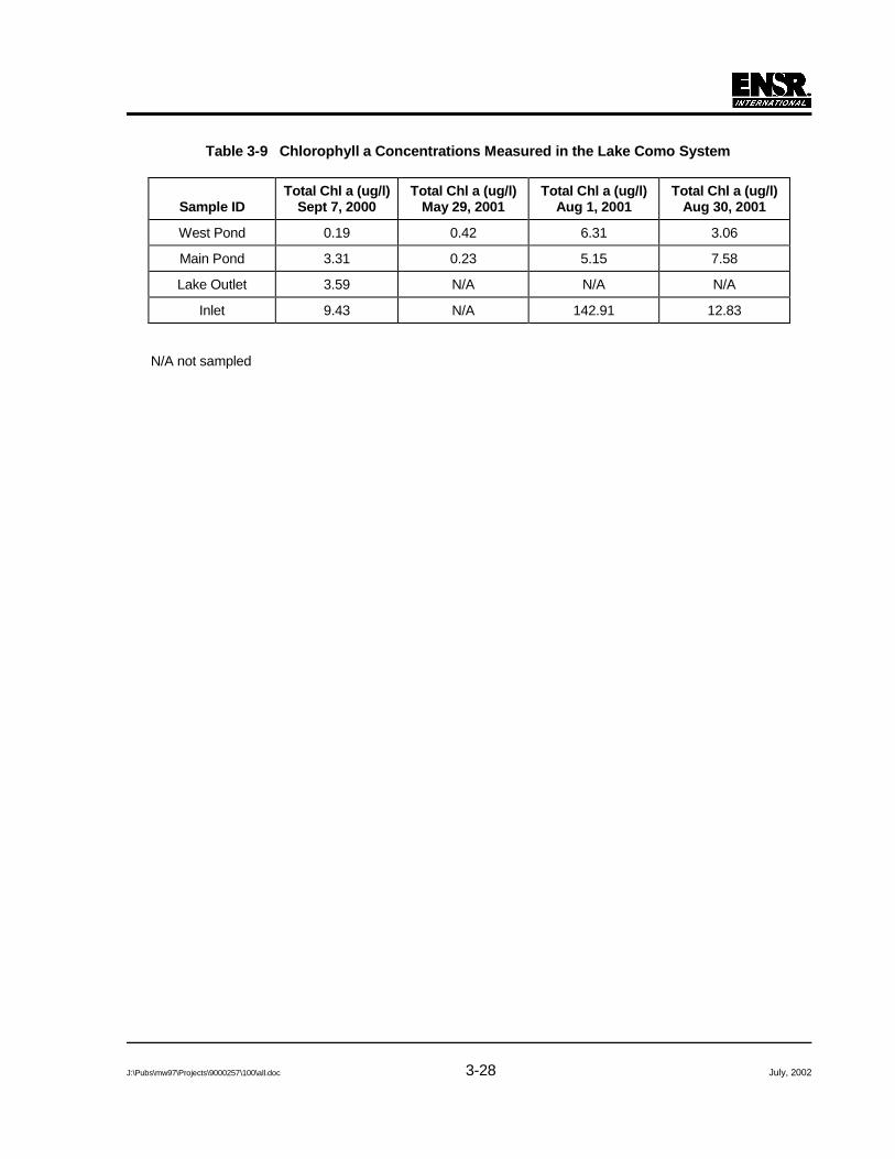
J:\Pubs\mw97\Projects\9000257\100\all.doc July, 20023-28
Table 3-9 Chlorophyll a Concentrations Measured in the Lake Como System
Sample IDTotal Chl a (ug/l)
Sept 7, 2000Total Chl a (ug/l)
May 29, 2001Total Chl a (ug/l)
Aug 1, 2001Total Chl a (ug/l)
Aug 30, 2001
West Pond 0.19 0.42 6.31 3.06
Main Pond 3.31 0.23 5.15 7.58
Lake Outlet 3.59 N/A N/A N/A
Inlet 9.43 N/A 142.91 12.83
N/A not sampled

J:\Pubs\mw97\Projects\9000257\100\all.doc July, 20023-29
Table 3-10 Sediment Chemistry Results for Sediments in Lake Como
MA Mean Lakeand Pond
Sediment Data
MA DEPBackground Soil
Data Set 90th
Percentile MCP RCS1Upstream
Lake ComoDownstreamLake Como
Nutrients (mg/kg)Kjeldahl Nitrogen 417E, SM 16th Ed. 1140 1210Phosphorus 4500-P-E-SM 18th Ed. 58 180Total Metals (mg/kg)Arsenic 6010B, SW-846 17.1 16.7 30 <7.18 8.18Cadmium 6010B, SW-846 4.6 2.06 30 <2.87 <1.36Chromium 6010B, SW-846 23 28.6 1000 8.80 15.1Copper 6010B, SW-846 41.8 37.7 1000 28.2 32.1Lead 6010B, SW-846 203 98.7 300 42.8 70.7Mercury 7471, EPA 1986 0.28 0.24 0.27Nickel 16.6 <28.7 <13.6Vanadium 28.5 <28.0 17Zinc 6010, EPA 1987 195 2500 69.0 119PCBs/Pesticides (ug/kg)Aldrin EPA 8080 <0.02 <0.02alpha-BHC EPA 8080 <0.015 <0.015beta-BHC EPA 8080 <0.03 <0.03delta-BHC EPA 8080 <0.045 <0.045gamma BHC (Lindane) EPA 8080 <0.02 <0.02Chlordane EPA 8080 <0.35 <0.354,4’-DDD EPA 8080 <0.055 <0.0554,4’-DDE EPA 8080 <0.02 <0.024,4’-DDT EPA 8080 <0.06 <0.06Dieldrin EPA 8080 <0.01 <0.01Endosulfan I EPA 8080 <0.07 <0.07Endosulfan II EPA 8080 <0.02 <0.02Endosulfan Sulfate EPA 8080 <0.33 <0.33Endrin EPA 8080 <0.03 <0.03Endrin Aldehyde EPA 8080 <0.115 <0.115Heptachlor EPA 8080 <0.015 <0.015Heptachlor Epoxide EPA 8080 <0.415 <0.415Methoxychlor EPA 8080 <0.06 <0.06Toxaphene EPA 8080 <1.2 <1.2PCB-1016 EPA 8080 <100 <100PCB-1221 EPA 8080 <100 <100PCB-1232 EPA 8080 <100 <100PCB-1242 EPA 8080 <100 <100PCB-1248 EPA 8080 <100 <100PCB-1254 EPA 8080 <100 <100PCB-1260 EPA 8080 <100 <100PCB-1268 EPA 8080 <100 <100TCMX (Surrogate) 69.9% 75.6%DCB (Surrogate) 71.9% 80.4%Petroleum Hydrocarbons 418.2, EPA 1983 95.0% 31.8%

J:\Pubs\mw97\Projects\9000257\100\all.doc July, 20023-30
Table 3-10 Sediment Chemistry Results for Sediments in Lake Como
MA Mean Lakeand Pond
Sediment Data
MA DEPBackground Soil
Data Set 90th
Percentile MCP RCS1Upstream
Lake ComoDownstreamLake Como
Polynuclear Aromatic Hyrdocarbons (mg/kg)Acenaphthene EPA 8270 20 <2.270 <1.200Acenaphthylene EPA 8270 100 <2.270 <1.200Anthracene EPA 8270 1000 <2.270 <1.200Benzo(a)anthracene EPA 8270 0.7 <1.140 <0.568Benzo(b)fluoranthene EPA 8270 0.7 <0.568 <2.990Benzo(k)fluoranthene EPA 8270 7 <0.568 <2.990Benzo(a)pyrene EPA 8270 0.7 <1.140 <0.568Benzo(g,h,i)perylene EPA 8270 100 <1.140 <0.568Chrysene EPA 8270 7 <1.140 <0.568Dibenzo(a,h)anthracene EPA 8270 0.7 <1.140 <0.568Fluoranthene EPA 8270 1000 <1.140 <0.568Fluorene EPA 8270 400 <3.410 <1.790Indeno(1,2,3-cd)pyrene EPA 8270 0.7 <1.140 <0.568Naphthalene EPA 8270 4 <2.270 <1.2002-Methyl Naphthalene EPA 8270 <1.140 <0.568Phenanthrene EPA 8270 100 <1.140 <0.568Pyrene EPA 8270 700 <3.410 <1.7902-Fluorobiphenyl (Surrogate) 47.0% 35.8%Nitrobenzene-D5 (Surrogate) 46.3% 35.4%Terphenyl-D14 (Surrogate) 65.5% 58.1%SolidsTotal Organic Carbon EPA 415.1 8.09% 8.01%Total Solids (ppm) 2540B SM 18th, 1992 7.77% 14.5%Total Volatile solids (ppm) 2540G SM 18th, 1992 65.0% 36.1%Percent Solids 8.3% 14.8%Grain Size% finer than 4.75 mm (Sieve Size 4) 100.0% 100.0%% finer than 2.00 mm (Sieve Size 10) 98.5% 99.5%% finer than 0.850 mm (Sieve Size 20) 92.5% 96.3%% finer than 0.425 mm (Sieve Size 40) 75.5% 81.1%% finer than 0.300 mm (Sieve Size 50) 67.0% 74.8%% finer than 0.180 mm (Sieve Size 180) 53.6% 57.9%% finer than 0.075 mm (Sieve Size 200) 35.4% 43.2%% > 3" 0.0% 0.0%% Gravel 0.0% 0.0%% Sand 64.6% 56.8%% Silt & Clay 35.4% 43.2%

J:\Pubs\mw97\Projects\9000257\100\all.doc July, 20023-31
Table 3-11 Summary of Aquatic Vegetation Investigation in Lake Como
Upstream Impoundment
TransectPoint
% Cover(see Legend)
% Biovolume(see Legend) Species Composition (%)
A-1 4 2 Wc(70), FG(30)A-2 4 2 Nv(30), Nitella flexilis(20), Najas flexilis(20), FG(20), Wc(10)A-3 4 3 Nitella flexilis(70), Nt(10), FG(10), Wc(10)A-4 4 2 Pp(60), FG(20), Nv(10), Wc(10)B-1 4 2 Nv(60), FG(30), Wc(10)B-2 4 1 Nv(50), Pp(20), FG(20), Wc(10)B-3 4 2 Nv(25), Pp(25), Nitella flexilis(25), FG(15), Wc(10)B-4 3 1 Nitella flexilis(50), Pc(10), Sl(10), Pp(10), Nv(10), FG(5), Wc(5), C-1 4 1 Pc(60), Nitella flexilis(20), Nv(10), FG(5), Wc(5), Lm(<5)C-2 4 2 Nv(30), Pp(30), FG(20), Nt(10), Wc(10), Lm(<5)C-3 4 2 Nv(70), FG(15), Wc(10), Lm(5)D-1 4 2 Nv(80), Wc(10), FG(10), Lm(<5)D-2 4 2 Nv(60), FG(20), Wc(10), Pp(5), Lm(5)E-1 4 1 Sl(40), Pc(30), Nv(10), FG(10), Wc(5), Lm(5)F-1 4 1 FG(50), Wc(50), Lm(<5)F-2 4 2 Nv(80), FG(10), Lm(10), Wc(<5)G-1 4 3 Pp(80), FG(10), Wc(10), Lm(<5)G-2 4 2 Nv(80), Wc(10), FG(10), Lm(<5)G-3 4 2 Nv(75), Wc(15), FG(10), Lm(<5)H-1 4 4 Nitella flexilis(70), Nv(10), Wc(10), FG(10), Lm(<5)H-2 4 4 Nitella flexilis(70), Nv(10), Wc(10), FG(10), Lm(<5)I-1 4 3 Nitella flexilis(40), Pp(40), Nv(10), FG(5), Wc(5), Lm(<5)I-2 4 4 Nitella flexilis(60), FG(20), Nv(10), Wc(5), Lm(5)
Downstream Impondment
TransectPoint
% Cover(see Legend)
% Biovolume(see Legend) Species Composition (%)
A-1 4 2 Cc(60), Ec(30), Wc(10)A-2 4 3 Cc(60), FG(30), Wc(10)A-3 4 1 Wc(50), Cc(50)A-4 4 1 Cc(50), Wc(25), FG(25)A-5 4 4 Cc(50), FG(40), Wc(10)B-1 4 4 Cc(60), Nt(30), Wc(5), FG(5)B-2 4 4 Cc(50), Us(40), Wc(5),FG(5)B-3 1 1 Cc(100)B-4 1 1 Cc(100)B-5 4 4 Cc(30), Nt(30), FG(30),Wc(10)C-1 4 2 Nt(60), FG(30), Wc(10)C-2 4 1 Nt(50), FG(40), Wc(10)C-3 4 4 Cc(60), FG(30), Wc(10)C-4 3 2 Cc(50), Us(30),FG(10),Wc(6),Lm(4)C-5 4 2 Nt(80), Wc(10), Cc(10)D-1 4 3 Nt(20),Cc(20), Ec(20), Mh(20), FG(10), Wc(6), Lm(4)D-2 4 4 Cc(50), FG(20), Mh(20), Wc(10)D-3 4 4 Mh(60), Cc(20), FG(10), Wc(10)D-4 4 4 Cc(80), FG(10), Wc(10)D-5 1 1 Cc(90), Wc(10)D-6 2 1 Nt(50), FG(40), Wc(10)E-1 4 1 Cc(40), FG(40), Wc(20)E-2 4 4 Nv(25), Cc(25), Mh(25), FG(15), Wc(10)E-3 4 4 Nv(25), Cc(25), Mh(25), FG(15), Wc(10)F-1 4 1 Wc(45), FG(45), Lm(10)G-1 4 1 FG(50), Wc(50)

Photo #1:North Attleboro Storm Drain.Downstream of Como Drive.
Photo #2:Attleboro Storm Drain.Downstream of Como Drive.
Photo #3:Main Basin Outlet.Upstream of Route 1.
Photo #4:Fuller HospitalStorm Drain.Downstreamof May Street.
Photo #7:West Basinlooking Upstream.
Photo #6:Main Basin Inlet.Downstream ofHeather Street.
Photo #5: Esker VillageStorm Drain.Downstream ofMay Street.
Figure 3-1Map ofLake Como
withPhotographs of Key Features
9000257100\fig3.1


J:\Pubs\mw97\Projects\9000257\100\all.doc July, 20024-1
4.0 WATERSHED ASSESSMENT
A watershed delineation and a land use identification evaluation were conducted in support of the LakeComo restoration study. Each evaluation is described below.
4.1 Watershed Delineation and Land Use Identification
The delineation of the Lake Como watershed was completed using scanned USGS 7.5-minutetopographic maps acquired from the MassGIS web site that houses geographic information forMassachusetts. The maps were imported into ArcView® and the area of the watershed wasdetermined by tracing the topography of the terrain that contributes flow to the outlet of Lake Como.The watershed area was divided into landuse types based on the MassGIS database of landuse.
Storm drains were identified during a site inspection, and using information provided by the City ofAttleboro Conservation Commission and the City of North Attleboro Conservation Commission.Because each storm drain was designed to receive overland runoff from a specific tract of land, thecontributing areas were determined either by storm drain permit inspection or topographic delineationof the area upgradient of each drain. No storm drains were identified for the West Pond. Three stormdrains and a small channel were identified for the Main Pond.
The area of the watershed contributing to the outlet of Lake Como is illustrated in Figure 4-1 and wasestimated to be 200 acres. The watershed is approximately 5,700 feet in length and has an averagewidth of approximately 1,500 feet. The watershed has a southeasterly aspect. Landuse in the basin ispredominantly residential except for the forested uplands and the Fuller Memorial Hospital, located tothe south of Lake Como.
There are four storm drain systems that discharge to the Main Pond of Lake Como: the Esker Villagedrain, the Fuller Memorial Hospital drain, Heather Street drain from North Attleboro, and the unnamedchannel discharging from Attleboro. The West Pond was inspected and no storm drains wereidentified to be discharging into Lake Como upstream of Como Drive (Figure 4-1).
• The drainage area of the Esker Village subdivision that contributes flow to Lake Como is 9.6acres. Stormwater is collected within the subdivision in storm drains and the water istransferred to the Main Pond immediately downstream of Como Drive through a concretepipe.
• The area of the Fuller Memorial Hospital that contributes stormwater to the lake is 24 acres.Similarly stormwater is collected in storm drains and is transferred to a clay pipe thattraverses May Street. This pipe is at least half filled with sediment and debris and flowthrough is severely restricted. Once stormwater from the hospital is on the north side ofMay Street it can flow overland to the Main Pond if the flow rate is sufficient.

J:\Pubs\mw97\Projects\9000257\100\all.doc July, 20024-2
• The area drained by the Heather Street drain in North Attleboro drains a residential areanorth of Lake Como and has an area of approximately 20 acres. This area is networkedwith a series of storm drains and storm sewer pipes to collect water throughout theresidential area. Flow is ultimately transferred to Lake Como Main Pond through a smallclay pipe. The pipe enters the lake immediately downstream of Como Drive.
• There is a fourth stormwater tributary to the Main Pond. The unnamed tributary is locatedon the north side of the main pond just west of Glen Street. This tributary appears to drainan approximately 5-acre area and is not associated with any storm sewer discharge. Thelocation for each of the four aforementioned stormwater discharges is indicated on Figure3-1.
4.2 Landuse and Historical Changes
In establishing landuse characteristics, ENSR evaluated MassGIS data that reports on landuse datafrom 1999. According to this data set, the landuse is approximately 42% low-density housing and 38%forested. Slightly less than ten percent of the land is designated open urban area (i.e. parks,easements, etc.) and slightly more than 5 percent of the watershed area is water. The remaining landis commercial, pasture, cropland, and wetland (0.68%, 0.56%, 1.3% and 1.5%, respectively).
As evidenced by the series of historical photographs (Appendix C), the uses of land in the Lake Comowatershed has changed substantially over the last 40 years. This is largely attributable to newhousing. The following bulleted list details some of the observations made during a comparison of themost recent aerial photo and the aerial photo dated April 22, 1959.
• On the north side of Lake Como, approximately 39 houses were counted in the 1959 photo.In the more current photo, ENSR identified approximately 64 houses in the sameneighborhood. Most of these houses were built on Campus Road and Loomis Street.
• On the south side of Lake Como, along the part of May Street shown, there wereapproximately 7 houses in 1959. The current photo shows approximately 15 houses alongthe same stretch of May Street.
• The vegetation observed along the bank edges of Lake Como in 1959 appears to begroomed low grasses with a smaller percentage of wetland plants, trees, and bushescompared to the current photo.
• The hospital grounds in 1959 included one large building, several small buildings, a smallparking lot and some cropland to the west of the hospital buildings. Since 1959, thehospital has expanded to approximately 8 more buildings, an additional parking lot, and anew driveway off May Street. The croplands to the west of the hospital buildings are nowthe new Esker Village neighborhood, at least 20 new houses.

J:\Pubs\mw97\Projects\9000257\100\all.doc July, 20024-3
• At the end of Campus Drive, there is a U-shaped feature that in 1959 appears to be a pond,and in the current photo appears to be a dry, shallow depression. The depression appearsdry in the 1971 photo and wet again in 1981.
• In the 1959 photo, there appear to be two stream channels at the headwaters of the westpond. The northern channel is wide and relatively open, compared to the southern channel,which is very straight and appears to be man-made. The more natural northern drainagefeature is not evident in the current photo. The straight channel is less distinct than in thepast but appears to be the dominant path of drainage from the upper, West Pond wetlands.The progressive overgrowth of the wider channel can be observed by looking at the picturesin series. It is not known who maintained this channel in the past.
• The difference in the area above the headwaters is minimal. There appear to be no newroads leading to new construction or development of the uplands to the west and north ofthe ponds.
The steady addition of residential homes and expansion of the Fuller Hospital area are likely two mainsources of increased rainfall runoff and resulting nutrient loading to Lake Como. The apparentredefining and straightening of the inlet channel has likely reduced the travel time and thus, the filteringtime by the wetland plants of the nutrient- rich water.
4.3 Description of Public Use Areas
A lakeshore reconnaissance survey was conducted to identify public use or access areas to LakeComo. One public use area was identified in the form of a small park along the southern shore of MainPond. The park extends approximately 500 feet along the southern shoreline across from the Hospital.The park includes a park bench, a narrow grassy area and a small semi-circular. The park does notinclude a boat launch, but a clearing exists allowing for small boat access (e.g., a canoe).
4.4 Watershed Assessment Summary
The Lake Como watershed assessment resulted in the following observations:
Physical Setting. The Lake Como drainage area is approximately 200 acres in size. The watershed isapproximately 5,700 feet in length and has an average width of approximately 1,500 feet. Thewatershed has a southeasterly aspect. Landuse in the basin is predominantly residential except forthe forested uplands and the Fuller Memorial Hospital located to the south of Lake Como.
Landuse. Based on the comparison of aerial photos dating back approximately 40 years to recentphotos and field observations, we can conclude that overall the runoff characteristics of the watershedhave most likely changed as a result of the increase in number of houses in this area. In the southeastportion of the watershed, the periodic additional development at Fuller Memorial Hospital is also likely

J:\Pubs\mw97\Projects\9000257\100\all.doc July, 20024-4
to cause changed runoff characteristics. Typically these kinds of developments increase runoff andnutrient loads to downstream receiving waters.
Drainage. A natural channel that flows south-southeast from the inlet through wetland to the WestPond drains the watershed. A culvert conveys water from the West Pond to the Main Pondunderneath Como Drive. Four drains convey storm flow from the upper portions of the watershed tothe Main Pond of Lake Como. They are as follows:
• Esker Village storm drain. Drains southwest subdivision. Approximately 9.6 acres.
• Fuller Memorial Hospital (Hospital) storm drain. Drains southeast urban open area.Approximately 24 acres.
• North Attleboro storm drains. Drains a residential area northwest of Lake Como.Approximately 20 acres.
• Attleboro drain. Drains a very small approximately 5-acre area and is not associated withany storm sewer discharge.
Results of the watershed assessment were applied to support the Lake Como watershed modelingapplication described below.


J:\Pubs\mw97\Projects\9000257\100\all.doc July, 20025-1
5.0 SCREENING LEVEL WATERSHED MODELING APPLICATION
A screening level watershed model based on landuse was applied to simulate average annual flowsand nutrient loads in the Lake Como system. The model was developed by ENSR and featuresapplication of several widely accepted watershed process estimation methods including those ofVollenweider (1968 and 1975), Kirchner and Dillon (1975), and others. A brief description of thewatershed modeling application is provided below and a detailed description is provided in AppendixD.
The Lake Como watershed model applies landuse-specific parameter values, such as runoff andexport coefficients (Reckhow et al., 1980), to estimate the load of water and nutrients to Lake Como.In-lake nutrient concentrations may then be estimated and the extent of nutrient reductions necessaryto achieve water quality improvement may be evaluated. Application of the screening level watershedmodel consists of a series of steps designed to allow the user to replicate the current watershed andin-lake situation and then evaluate alternative management scenarios to improve in-lake water quality.The following watershed modeling steps were undertaken as part of the Lake Como watershedevaluation.
1. Delineation of watershed and subbasin boundaries
2. Determination of average flow using runoff coefficients
3. Determination of nutrient loads using export coefficients
4. Estimation of in-lake nutrient concentrations
5. Estimation of nutrient goals in terms of permissible and critical nutrient concentrations
Each of these modeling steps is described in Appendix D including associated governing equationsand literature sources.
5.1 Model Setup
Setup of the landuse based watershed model requires knowledge of the individual subbasins withinthe overall drainage basin, including the size of these watersheds, landuses within them, the overalldrainage pattern, and any other features that could increase or decrease nutrient loads. The LakeComo watershed was divided into subbasins that each represent the inflow from tributaries, stormdrains and direct groundwater flow to Lake Como. The landuses for each of the subbasins wasdetermined using information from the Massachusetts GIS Internet site(http://www.magnet.state.ma.us/mgis/), with field inspection for verification. Precipitation data was

J:\Pubs\mw97\Projects\9000257\100\all.doc July, 20025-2
obtained from the National Weather Service gauging station in Boston, MA and applied to the LakeComo watershed modeling application.
Median precipitation runoff or export coefficient values for each land use in the Lake Como watershedwere initially selected and applied based on available data and best professional judgment.Attenuation coefficients were selected according to expected removal efficiency associated withmapped features of the watershed and stream system. Information on lake features was derived frommaps and field surveys.
5.2 Model Development
The model development process involved applying the screening-level Lake Como watershed model,and adjusting model parameter values, to improve the accuracy of flow and nutrient load predictions ofcurrent conditions. Water quality data collected during the field investigation were applied to developand establish a crude calibration of the screening level watershed model. Nutrient concentrationspredicted by the model at the discharge point in each watershed were compared to available field data.Model parameter values were also compared with appropriate literature values to insure thatreasonable values were applied to the model. The model development process resulted in selection ofrunoff, export, and attenuation coefficient values, that collectively resulted in reasonablerepresentations of current Lake Como watershed processes on an average annual basis.Development of the screening level landuse model was designed to achieve the following two goals:
1) Adjust watershed export and attenuation coefficients within literature-defined range for eachlanduse or attenuator type so an optimal match between model predicted and field measurednutrient concentrations, at key points in the system, is obtained.
2) Establish an optimal match between model predicted and field measured in-pond nutrientconcentrations.
Model development was successfully completed. Model predicted and actual in-stream values wereacceptably similar. It should be noted that this is a screening level model and model predictionsshould be interpreted as rough estimates of actual site conditions. The predictions are very useful,however, for evaluating and comparing expected water quality improvements associated with variouspond restoration alternatives.
The model was applied to predict flows and nutrient concentrations associated with each stormwatersource and tributary. Annual average flows and nutrient loads were then predicted using theprecipitation record for the area obtained from the National Weather Service gauge in Boston, MA.

J:\Pubs\mw97\Projects\9000257\100\all.doc July, 20025-3
5.3 Hydrologic Simulation Results
The Lake Como model was applied to estimate mean turnover rate and residence time and to estimatethe relative contribution of each water source to the Lake Como system. Each of these hydrologiccalculations is described below.
5.3.1 Lake Como Mean Turnover Rate and Residence Time
Mean turnover rate and residence time values are hydrologic metrics describing the relationshipbetween the volumetric rate of water entering the pond and the total pond volume. Turnover rate andresidence time values can provide insights on the quality of a pond habitat and its ability to supportdiverse animal and aquatic plant communities.
Turnover rate is defined as the number of times that the total volume of water in the lake is exchangedduring a unit period of time. The turnover rate is defined as the volumetric rate of water entering thelake divided by the lake volume. Water entering the Lake Como was represented as watershed runoffand neglected groundwater inflow/outflow and evaporation processes. Turnover rates may beestimated on an annual and/or seasonal basis since the effects of the turnover rate are usually theresult of seasonal differences in precipitation. Shorter-term calculations can be made to identify theturnover rate associated with a particular storm. Residence time is defined as the inverse of turnoverrate and expresses the period of time that a water parcel remains in the pond assuming all watermoves through the pond at the same rate.
Table 5-1 presents turnover rate and residence time estimates in Lake Como for each of four periodsincluding the spring, summer, annual, and for a 24-hour storm with a 1-year return period. Runoffrates were determined by multiplying the average annual runoff coefficient by the runoff duration. Theaverage annual runoff coefficient was determined by dividing the average annual runoff (33.5 in/yr),determined in the spreadsheet model, by the average annual precipitation (44.9 in/yr).
During the spring and summer seasons, Lake Como turns over approximately 5 times with a meanresidence time of 17 days. On an annual basis, the lake is estimated to turn over 24 times with amean residence time of 15 days. Lastly, a major precipitation event, the one-year storm, results in onecomplete exchange of water in the Lake Como system – flushing out the entire lake volume in oneday.
5.3.2 Flow Budget for Lake Como Watershed
The Lake Como screening level watershed model was applied to estimate the flow budget of LakeComo on an average annual basis. The flow budget was developed using the results of the watershedmodel under present conditions. As described in the watershed assessment (Section 5), the LakeComo watershed may be represented as six separate subbasins for the purposes of watershed

J:\Pubs\mw97\Projects\9000257\100\all.doc July, 20025-4
landuse-based modeling. These subbasins included the areas contributing to the North Attleboro,Attleboro, Hospital, and Esker Village stormdrains, and the remaining West and Main Ponds.
The estimated annual flow budget for the Lake Como watershed is summarized in Table 6-2. The flowbudget developed using the Lake Como spreadsheet model indicates that approximately 72% of the689 acre-ft/yr of precipitation (44.9 in/yr) was accounted for as direct runoff. Additionally, the annualET accounts for 30% of the water loss from the basin. The groundwater inflow to the basin wasaccounted for by calculating the difference between the precipitation and the runoff and ET from thebasin. Groundwater inflow amounted to a loss of 2% from the water budget.
5.4 Water Quality Simulation Results
The Lake Como model was applied to estimate the relative contribution of nutrient loads for each watersource to the Lake Como system. The nutrient load estimation process was conducted on an annualaverage basis for current conditions. Next, phosphorus reduction goals were established for the LakeComo system based on a widely accepted assessment method. The screening-level Lake Comowatershed model was then applied to evaluate the potential for each of several restorationmanagement alternatives to improve water quality in the Lake Como system. Each of these waterquality assessment tasks is described below.
5.4.1 Assessment of Present Phosphorus Loads
The Lake Como screening level watershed model was applied to estimate the phosphorus budget ofLake Como on an average annual basis. The phosphorus budget was developed using the results ofthe watershed model under current conditions. Phosphorus loads were derived for each of the sixsubbasins within the Lake Como watershed. External sources of phosphorus were assumed toinclude atmospheric loading and a load from waterfowl. Phosphorus loads from each subbasincomponent were predicted by applying landuse based export coefficients to each of the subbasins.Phosphorus concentrations were then calculated by dividing the predicted phosphorus load by thepredicted volumetric flow rate from each subbasin (presented in Section 5.3.2 above). Theatmospheric load of phosphorus to the surface of Lake Como was assumed to be 0.4 kg/yr and thewaterfowl load to the lake was estimated to be 3 kg/year.
The estimated annual flow budget for the Lake Como watershed is summarized in Table 5-3. Thepredicted phosphorus load from each source indicates that nearly all sources of phosphorus to LakeComo come from the surrounding subbasins (96%). Subbasin areas contributing the most annualphosphorus load were the areas contributing to the West Pond (31%), the Hospital stormdrain (21%),and the North Attleboro stormdrain (19%). Phosphorus contributions from the remaining threesubwatersheds were considerably less (5-12% each) and loads from external sources werecomparatively minor (<4%).

J:\Pubs\mw97\Projects\9000257\100\all.doc July, 20025-5
5.4.2 Phosphorus Reduction Goals for the Lake Como System
An assessment method developed by Vollenweider (1968) was applied to Lake Como to provide anestimate of the extent of nutrient reduction that would likely be necessary to remove water quality andbiological impairment from the Lake Como system. Permissible and critical limits for phosphorus loadswere estimated where the permissible load is defined as the amount of phosphorus that could enter asystem without having obvious or continual detrimental effects. In other words, if permissible levels ofnutrients are present, then the waterbody is not likely to be impaired. The critical limit is defined astwice the permissible load. If critical levels of nutrients are present, then the waterbody is likely to beimpaired. In general, as nutrient concentrations exceed the permissible load level and approach thecritical load level, nuisance algal blooms and other aquatic biological activity can become problematic.Lakes exceeding the critical load typically experience serious productivity problems.
For the Lake Como application, the Vollenweider method was applied and permissible and criticalphosphorus loads for Lake Como were calculated to be 11 and 22 kg/yr, with corresponding in-lakeconcentrations of approximately 16 and 31 µg/L, respectively. The permissible and critical nutrientload estimation process is a screening level tool and additional factors, such as the physicalcharacteristics of the lake system should also be evaluated.
A review of phosphorus measurements collected during the Lake Como field investigation indicates anaverage in-lake phosphorus concentrations averaged 90 µg/L (see Table 3-1 summary statistics). TheLake Como watershed model predicted total annual phosphorus loadings of 109 lbs/yr. Phosphoruslevel in the ponds and phosphorus loads from the watershed are both well above the predictedpermissible and critical phosphorus concentrations and suggests that phosphorus levels must bereduced by approximately a factor of 5 before water quality impairment may be removed from LakeComo. Thus, restoration alternatives will need to be selected and applied to reduce phosphorusconcentrations dramatically, if water quality standards and designated use goals are to be attained.
5.4.3 Model Simulation Results for Restoration Alternatives
Presently, phosphorus concentrations in Lake Como are sufficient to lead to water quality impairment.The Lake Como watershed model was applied to evaluate several restoration alternatives for reducingnutrient loads. The watershed model is designed to evaluate watershed runoff of water and nutrientsand to estimate in-lake nutrient concentrations, given specified physical characteristics. Thus, themodel is capable of estimating water quality improvements associated with modifications to sources ofnutrients. The model is not well suited however, to provide accurate predictions of water quality effectsassociated with other restoration alternatives, such as modifications to impoundment dams ordredging. These restoration alternatives are important for Lake Como and will be discussed in“Section 6 - Management Goals and Recommendations”, but are not evaluated using the watershedmodel.

J:\Pubs\mw97\Projects\9000257\100\all.doc July, 20025-6
A total of 4 restoration alternatives were simulated using the watershed model and predictedreductions in total nutrient loading were obtained. Predicted reductions in phosphorus loads arerelative to present loads (presented in Table 5-3). Descriptions and modeling results for eachrestoration alternative scenario are provided below.
Scenario 1: Remove All Storm Drain Flow. This scenario specifies redirecting all storm drain flowout of the watershed (downstream of Main Pond watershed). This restoration alternative would requirererouting storm drain flow via a set of pipes to connect stormdrains to the Route 1 storm drain network,just below the main pond dam. An engineering feasibility assessment would likely be required toevaluate a set of options for removing all storm drain flow and to estimate the total cost of the project.
The scenario 1 restoration alternative was predicted to result in a 50% decrease in total annualphosphorus load to Lake Como.
Scenario 2: Infiltrate All Storm Drain Flow. This scenario specifies installation of an infiltrationsystem for all storm drains to attenuate nutrient load to the waterbody. This restoration alternativewould require construction of detention basins and/or dry wells to enable stormwater to infiltration togroundwater, rather than being transported directly to Lake Como. Stormwater infiltration systemshave been demonstrated to be highly effecting in removing nutrients from storm flow.
The scenario 2 restoration alternative was predicted to result in a 40% reduction in total annualphosphorus loading to the Lake Como system.
Scenario 3: West Pond Wetland Conversion. This scenario specifies that the West Pond beallowed to revert to a wetland. This restoration alternative would increase the capacity of West Pondto attenuate nutrients prior to being released into the Main Pond. The tradeoff associated with thisalternative involves allowing West Pond to degrade from a pond to a wetland in exchange forimproving water quality in the Main Pond.
The scenario 3 restoration alternative was predicted to result in a 10% reduction in total annualphosphorus loading to Lake Como. Other processes not accurately simulated by the model, such asretention of nutrients by wetland vegetation, and hydrologic modification in West Pond, may result ingreater phosphorus load reductions than those predicted.
Scenario 4: West Pond Wetland Conversion and Infiltrate Storm Drain Flow. This restorationalternative is a combination of Scenarios 2 and 3 above – featuring conversion of West Pond to awetland and installation infiltration system for all stormwater drainage.
The scenario 4 restoration alternative was predicted to result in a 50% reduction in total annualphosphorus loading to Lake Como.

J:\Pubs\mw97\Projects\9000257\100\all.doc July, 20025-7
Summary of Model Scenarios
The model was applied to evaluate restoration alternatives for stormwater drains and tributaries in theLake Como system. Restoration management alternatives featuring removal of stormdrain dischargesor groundwater infiltration of discharges were predicted to result in 40% to 50% reductions in totalannual phosphorus loads to Lake Como. These reductions alone would not be sufficient tosubstantially reduce water quality impairment, based on phosphorus reduction goals for the LakeComo system. A combination of restoration alternatives featuring watershed nutrient reductions, asdescribed above, and other alternatives, such as dam repair and dredging, may be required to achievethe necessary water quality improvements in the Lake Como system. A discussion of managementalternatives and recommendations is provided below.
5.5 Summary of Watershed Modeling Results
The watershed modeling application provided the following insights on the Lake Como system:
• Pond Hydrologic Assessment - The hydrologic assessment of Lake Como indicated that themean turnover rate in Lake Como is approximately 5 times per season during the springand summer (residence time 17 days). Also, the one-year storm was estimated to result inone complete replacement of pond volume (residence time 1 day).
• Watershed Phosphorus Load Budget – The average annual phosphorus load wasestimated to be approximately 105 kg/yr. The sources of phosphorus were as follows (with% contribution shown: 31% from runoff directly to West Pond (via tributary and overland);21% from the Fuller Hospital storm drain; 19% from the North Attleboro storm drain; 12%from runoff directly to the Main Pond; 8% from the Esker Village storm drain; and 5% fromthe Attleboro storm drain.
• Target Phosphorus Loading and In-Lake Goals - Widely accepted methods were applied todevelop target phosphorus load and in-lake goals. A total annual phosphorus load goal of11 to 22 kg/yr was established and an in-lake phosphorus concentration goal of 16 to 31µg/L was established. Comparison of phosphorus targets to watershed model predictionsof phosphorus loads and field measurements of in-lake concentrations indicates thatphosphorus concentration must be reduced by approximately a factor of 5 (i.e., 5 times lessload) before water quality improvement may be achieved.
• Evaluation of Restoration Alternatives – Restoration alternatives featuring reduction orremoval of storm drain loads were evaluated using the watershed model. Removal orinfiltration of storm drain flows from the system was predicted to result in 40% to 50%reductions in average annual loads of phosphorus to the ponds. These modifications wouldhave to be implemented along with additional modifications in order to achieve necessarywater quality improvements.

J:\Pubs\mw97\Projects\9000257\100\all.doc July, 20025-8
The management goals and recommendations section, below, provides a complete description ofrecommended restoration activities for the Lake Como system.

J:\Pubs\mw97\Projects\9000257\100\all.doc July, 20025-9
Table 5-1 Lake Como Hydrology: Estimated Turnover Rates and Residence Times
DurationTotal
Precipitation (in)ResidenceTime (days)
Number ofTurnovers
Spring (3 months) 10.2 17 5.5Summer (3 months) 9.8 17 5.3
Annual 44.9 15 24.324-hour 1-year storm 1.7 1 0.9

J:\Pubs\mw97\Projects\9000257\100\all.doc July, 20025-10
Table 5-2 Lake Como Hydrology: Estimated Water Budget
Parameter Value PercentPrecipitation (acre-ft/yr) 689 100%Total Runoff (acre-ft/yr)• North Attleboro Storm Drain (acre-ft/yr)• Attleboro Storm Drain (acre-ft/yr)• Hospital Storm Drain• Esker Village Storm Drain• Contribution to West Pond• Contribution to Main Pond
497• 67• 17• 59• 33• 268• 52
72%• 10%• 3%• 9%• 5%• 39%• 8%
1Evapotranspiration (acre-ft/yr) 207 30%2Groundwater (acre-ft/yr) (15) (2%)1Half of Potential ET (from Water Atlas, 1973)2Precipitation = Runoff + ET + Groundwater

J:\Pubs\mw97\Projects\9000257\100\all.doc July, 20025-11
Table 5-3 Lake Como Water Quality: Estimated Phosphorus Budget
Phosphorus Loading Component Value PercentAtmospheric Deposition (kg/yr) 1.2 1.1%Total Watershed Load (kg/yr)• North Attleboro Storm Drain (kg/yr)• Attleboro Storm Drain (kg/yr)• Hospital Storm Drain (kg/yr)• Esker Village Storm Drain (kg/yr)• Contribution to West Pond (kg/yr)• Contribution to Main Pond (kg/yr)
105• 21• 5• 23• 9• 34• 13
96%• 19%• 5%• 21%• 8%• 31%• 12%
Waterfowl (kg/yr) 3 2.8%
Total Load of Phosphorus to Lake (kg/yr) 109 100%

J:\Pubs\mw97\Projects\9000257\100\all.doc July, 20026-1
6.0 MANAGEMENT GOALS AND RECOMMENDATIONS
Observations of existing problems, documented as part of the Lake Como Restoration Study, arestated below followed by a statement of lake restoration goals. The description of existing problemsand goals provides context for presentation and discussion of a set of management recommendationsfor the Lake Como system presented in Section 7.3 below.
6.1 Observations of Existing Problems
The following existing problems were observed in the Lake Como system:
• Low water levels during the summer in the main basin.
• Excessive concentrations of phosphorus, nitrogen, and other pollutants in stormwaterentering the ponds.
• Excessive concentration of phosphorus, nitrogen, suspended solids and other pollutants inthe water column in the ponds.
• Extensive aquatic vegetation primarily aquatic macrophytes on the water surface and in thewater column of the ponds
• Soft, nutrient-rich sediments supporting growth of rooted plants that impede recreationalactivities.
6.2 Lake Como Restoration Goals
Lake Como restoration goals include the following:
• Improve water quality to enable the ponds to achieve the water quality standards associatedwith its designated use. Specifically, enable the ponds to meet numeric criteria for ambientdissolved oxygen concentration and narrative criteria for nuisance aquatic vegetation;
• Enable passive uses of the ponds for non-motorized boating;
• Improved visual aesthetics, with reduced odor and unsightly growths; and
• Restore the habitat of the ponds to support fish and wildlife populations.
Restoration management plans designed to support achievement of these goals are described below.

J:\Pubs\mw97\Projects\9000257\100\all.doc July, 20026-2
6.3 Management Recommendations
A complete management program should include watershed and in-lake components, as individualcomponents do not appear to provide for optimal long-term conditions in Lake Como. ENSR hasevaluated a variety of management options for Lake Como and identified the following 4recommended restoration tasks:
1. Repair leaky dam to support increased pond volume and water level.
2. Dredge nutrient-rich pond sediments to reduce sources of excess biological growth and increasepond volume.
3. Reduce nutrient loading to ponds through infiltration or removal of stormwater sources.
4. Develop a watershed education program to provide interested parties with information necessaryto reduce point and non-point sources of nutrients in the Lake Come watershed.
A description of each of these 4 recommended restoration alternatives is provided below. Allalternatives explored as part of the Lake Como Management Alternatives Analysis are provided inAppendix E of this report. Included in Appendix E are also some suggested Best ManagementPractices that could be employed within the watershed (i.e. catch basin clean outs, public education,etc.).
6.3.1 Repair of Leaky Dam to Maintain an Appropriate Pond Water Level
Repairing the outlet structure is a logical option for raising the water level and improving habitat in MainPond; however, ownership of the dam will need to be determined by the City of Attleboro.Reconstruction of the outlet along Route 1 would facilitate up to a 3 foot increase in the water level in acost-effective manner. Repair of the outlet structure should include construction of an antechamberwith flashboards in front of the current outlet area. This design would provide flexibility to manage thepond in response to flood conditions and to keep water levels as high as possible during dry periods.The repaired outlet structure would 1) normally hold the water level close to full level, 2) minimize waterlevel rise during storms, and 3) facilitate drawdown for maintenance or plant control by flashboardremoval.
Installation of such a new outlet would constitute a major overhaul of the existing structure, but couldbe permitted as dam maintenance as it would occupy almost the same footprint and have the sameintent as the original structure. Permitting through the Attleboro Conservation Commission under theWetlands Protection Act is essential, and Section 401 and 404 permits may or may not be necessary,depending upon regulatory interpretation. No Great Pond provisions of MA law apply, and it seemsunlikely that the current dam is even listed as a permitted structure. Filing through the Dam Safety Unit

J:\Pubs\mw97\Projects\9000257\100\all.doc July, 20026-3
of DEM may not be necessary, but that group should be contacted for input. The cost of such anupgrade is difficult to estimate at this time, but might be expected to be in the range of $50,000 to$100,000, inclusive of design and permitting expenses.
6.3.2 Dredge to Reduce Excess Growth of Aquatic Vegetation
While raising the water level will be a definite aid to improving pond appearance, the existing organicsediment deposits and nutrient-rich influent will continue to support dense plant growths and continuedalgal mat production. Dredging the ponds, or at least the Main Pond, to remove the accumulatedorganic sediment is the preferred approach to restoring the ponds. Accumulated organic sediment ofapproximately 7,850 cubic yards in the Main Pond and 4,830 cubic yards in the West Pond should becompletely removed in order to reduce plant and algal mat growths to aesthetically appealing levels.Such dredging would also improve the habitat for most desirable forms of aquatic life. Plants wouldnot be eliminated, but densities should be reduced by approximately 75%, likely creating better openwater habitat for fish and enhancing habitat value for birds, reptiles and amphibians.
Assuming that the outlet is to be reconstructed, it would make sense to drain the pond, at which timedredging could be conducted. If it is desired that both ponds be reclaimed, both could be dredged atonce, but it would be logistically and ecologically appropriate to do them sequentially to provide arefuge for fish and wildlife during the process. The West Pond would be dredged first, as the upstreamimpoundment, followed by the Main Pond. Wet weather may limit in-situ dewatering, but it doesappear that this project can be carried out without an overly sophisticated dredging plant. Two accessramps can be established for each pond and restored later to avoid any permanent damage to bankresources. Conventional excavation equipment should be able to enter each pond and work from theedge, possibly from mats at first, clearing the bottom of soft sediment. Temporary storage may beneeded, and the feasibility of using the parkland or part of the adjacent hospital grounds should beexplored. Sediment appears to be of sufficiently high quality to be trucked to a variety of productiveuse sites without regulatory problems.
In dry condition, the sediment that now occupies almost 12,000 cyds will not likely have a volume morethan 3,000 to 4,000 cyds, but getting it into that dry condition will require either spreading it thinly orapplying enhanced dewatering techniques. Having sufficient temporary storage or a permanentdisposal site where water content does not matter (e.g., a former gravel pit) will be important tomaterial utility and cost control.
The cost of dredging depends on a wide range of site-specific factors, but experience has shown that acost range from $5 to $30 per cyd is typical, with higher or lower values possible where the materialhas substantial resale value or where contamination and distance to the disposal site are majorfactors. A typical rough estimate of $10 per cyd is often assumed to provide some indication ofpossible level of expense, suggesting a cost of about $120,000 in this case. Permitting would includean Order of Conditions under the Wetlands Protection Act and Section 401/404 permits, at a minimum.

J:\Pubs\mw97\Projects\9000257\100\all.doc July, 20026-4
An ENF (Environmental Notification Form) would be required for the proposed dredging project sincedredged material is estimated to exceed 10,000 cyds. The Secretary would then determine if an EIR(Environmental Impact Report) would be required. However, a Request for Determination should befiled with MEPA (Massachusetts Environmental Policy Act) once the details of the project have beendetermined. MEPA could rule that dredging of Lake Como is "Routine Maintenance" in which case anENF and an EIR would not be required. Therefore, selection of temporary and permanent disposalsites would be the next logical step in pursuing this option.
6.3.3 Reduce Nutrient Loads to Ponds
Reductions of nutrient loads to ponds were evaluated using the screening level Lake Como watershedmodel and are summarized in Section 5. Nutrient loads must be reduced, along with repair of theoutlet structure and dredging, to ensure that the ponds do not quickly revert to present conditions.Failure to address incoming water quality concerns could result in only temporary improvement or insubstitution of one problem for another (e.g., algal blooms instead of plant nuisances). The watershedmodeling management scenarios clearly indicate that small efforts will not provide the level ofimprovement in water quality necessary to make a difference in the lake, at least in terms of nutrientlevels. It will be necessary to manage most runoff to a high degree, although this problem cancertainly be attacked over time, discharge by discharge.
Infiltration, detention, and/or redirection of storm water would appear to have the greatest potential forachieving the goal of dramatic reduction in nutrient loads to the ponds. The design of infiltrationsystems will depend upon the site specific conditions, most especially soil permeability and depth togroundwater. It appears that some form of lateral system may be needed for each of the four majordrainage systems entering the Main Pond, to ensure infiltration of as much runoff as possible.Positioning under existing lawn areas may be appropriate, and simple leaching catch basins could beinstalled in some cases. Assuming that all four current discharges are addressed with leachingsystems that incorporate capture of the first half inch of runoff, pre-settling basins (to minimizeclogging), and a laterally oriented infiltration system to avoid any shallow ground water problems), thecost is likely to be on the order of $120,000. Simpler systems may be applicable, if soil conditions aresuitable.The design of an upstream detention system must maximize detention and associatedpollutant retention processes while minimizing flood problems around the detention area. Establishinga detention basin at the upstream end of the West Pond appears feasible, although permitting underthe Wetlands Protection Act is not guaranteed. Detention further upstream, possibly by expandingwetlands along the stream corridor, may have greater merit. Given the watershed area upstream ofthe West Pond, the detention area should be about 3 acres in size. The cost of an appropriatedetention system is estimated at approximately $50,000, if done as a habitat-enhancing wetland. Anyland purchase costs would be in addition to the $50,000.Watershed Education Program
A watershed education program should be developed and made available to interested parties,particularly residents within the Lake Como watershed. The program should, at a minimum, offer clear

J:\Pubs\mw97\Projects\9000257\100\all.doc July, 20026-5
and concise recommendations to area residents and businesses that will enable them to effectivelyreduce nutrient loads around the watershed. The program should clearly indicate the current state ofthe watershed and the benefits that can be achieved through the use of Best Management Practices(BMPs).

J:\Pubs\mw97\Projects\9000257\100\all.doc July, 20027-1
7.0 REFERENCES
Dillon, P.J. and F.H. Rigler. 1974. The phosphorus-chlorophyll relationship in lakes. Limnol.Oceanogr. 19:767-773.
Esker Corp. 1997. Esker Village Drainage Calculations. Prepared for Esker Corporation. PreparedBy W.T. Whalen Engineering Co., North Attleboro, MA and Carr Research Laboratory, Inc., Wellesley,MA.
Geraghty, J.J., D.W. Miller, F. van der Leeden, F.L. Troise. 1973. Water Atlas of the United States.Water Information Center Inc., Water Research Building, Port Washington NY.
Godfrey, P. (1988). Acid rain in Massachusetts. WRRC, UMASS, Amherst.
Hellquist G. B., & Crow G. E., 1980. Aquatic Vascular Plants of New England: Part 1. Zosteraceae,Potamogetonaceae, Zannichelliaceae, Najadaceae. Publication #515 of the New HampshireAgricultural Experiment Station of the University of New Hampshire, Durham, NH.
Hellquist G. B., & Crow G. E., 1982. Aquatic Vascular Plants of New England: Part 5. Araceae,Lemnaceae, Xyridaceae, Eriocaulaceae, and Pontederiaceae. Publication #523 of the NewHampshire Agricultural Experiment Station of the University of New Hampshire, Durham, NH.
Jones, J. and R. Bachmann. 1976. Prediction of phosphorus and chlorophyll levels in lakes. JWPCF48:2176-2184.
Jones, R.A., W. Rast and G.F. Lee. 1979. Relationship between summer mean and maximumchlorophyll a concentrations in lakes. Env. Sci & Technol. 13:869-870.
Kirchner, W. and P. Dillon. 1975. An empirical Method of estimating the retention of phosphorus inlakes. Water Resourc. Res. 11:182-183.
Larsen, D. and H. Mercier. 1976. Phosphorus retention capacity of lakes. J. Fish. Res. Bd. Can.33:1742-1750.
Massachusetts Department of Environmental Protection (MA DEP) Working Document. PALISDatabase. MA DEP, Boston, MA.
Massachusetts Department of Environmental Protection (MA DEP), 1995. 310 CMR. Guidance forDisposal Site Risk Characterization. MA DEP, Boston, MA. (includes background soil concentrations)

J:\Pubs\mw97\Projects\9000257\100\all.doc July, 20027-2
Massachusetts Division of Water Pollution Control. (1993). 314 CMR: Division of Water PollutionControl (Section 4.00 Massachusetts Surface Water Quality Standards).
McKee, J. E., and H. W. Wolf. (1963). Water quality criteria (Publ. #3-A). Sacramento, CA: StateWater Res. Control Bd.
McNaughton, S.L. and L. L. Wolf. General Ecology. 1973. Holt, Rinehardt and Winston, Inc. New York,NY.
Oglesby, R.T. and W.R. Schaffner. 1978. Phosphorus loadings to lakes and some of their responses.Part 2. Regression models of summer phytoplankton standing crops, winter total P, and transparencyof New York lakes with phosphorus loadings. Limnol. Oceanogr. 23:135-145.
Reckhow, K.H., M.N. Beaulac, and J.T. Simpson. 1980. Modeling phosphorus loading and lakeresponse under uncertainty: A manual and compilation of export coefficients. EPA 44015-80-011.
Vollenweider, R. A. (1968). Scientific fundamentals of the eutrophication of lakes and flowing waters,with particular reference to nitrogen and phosphorus as factors in eutrophication. Paris, France: Tech.Report to OECD.
Vollenweider, R. 1968. Scientific Fundamentals of the Eutrophication of Lakes and Flowing Waters,with Particular Reference to Nitrogen and Phosphorus as Factors in Eutrophication. Tech. Rept. ToOECD, Paris, France.
Vollenweider, R. 1975. Input-output models with special reference to the phosphorus loading conceptin limnology. Schweiz. Z. Hydrol. 37:53-62.
Vollenweider, R.A. 1982. Eutrophication of Waters: Monitoring, Assessment and Control. OECD, Paris,France.
Wetzel, R.G. (1983). Limnology (2nd ad.). Orlando, Fl: Saunders College Publishing.
Wetzel, R. G. (1975). Limnology (1st ed.). Philadelphia, PA: Saunders Co.

APPENDIX A
PHOTOS OF STORM DRAINS AND OUTLET STRUCTURE


Ken Wagner, ENSR 508-393-6779
CHECKLIST OF LAKE MANAGEMENT STUDY ELEMENTS
Lake Management study elements are listed below.
Lake Management ObjectivesExisting and desired usesPriority of usesSpecial features or considerations
Watershed FeaturesPhysicalArea, topography, drainage basinsSoils and geologyLand use and vegetationStormwater drainage systemsWaste disposal practicesOther pollution sourcesHistorical informationFlow estimates (precipitation, evaporation, surface flows, groundwater, discharges,withdrawals)
ChemicalNutrient levels – total P, dissolved P, nitrate N, ammonium N, total Kjeldahl NpH/alkalinityTurbidity/suspended solidsConductivity/dissolved solidsTemperature/dissolved oxygenPotentially toxic compounds - anything suspected?
Lake FeaturesArea, shape, morphometry (depth map)Volume, mean/maximum depthsDetention time, response timeWater chemistry (parameters as for watershed, plus water clarity)Temperature/oxygen (top and bottom, 1 m intervals if deeper than about 15 ft)Soft sediment distribution, physical features (muck, sand, gravel)Sediment chemistry – N, P, selected metals, TPH, PAHs, organic content, solidscontent, grain sizeBiology (bacteria, algae, macrophytes, zooplankton, benthic invertebrates, fish,amphibians, reptiles, birds, mammals)

Ken Wagner, ENSR 508-393-6779
CHECKLIST OF LAKE MANAGEMENT STUDY ELEMENTS (continued)
Loading Analysis (water and contaminants)Atmospheric inputsDry weather surface waterStorm waterGround waterInternal recycling (release from sediment0Waterfowl and other wildlifePoint source dischargesPermissible/critical loadsRelationship between loads, concentrations, and algae/water clarityDesired reduction and expected results
Management AssessmentProblem definitionReview of applicable techniquesIdentification of appropriate techniquesSelection of management plan elements
Management Plan DevelopmentTechnical implementation strategyRegulatory requirementsCost estimatesImplementation scheduleFurther data needs and monitoring program


Description of Screening Level Lake Como Watershed Model
The landuse based spreadsheet model, developed by ENSR and applied to the Lake Como system,facilitates the development of a nutrient budget for Lake Como and the associated watershed. Themodel uses landuse specific runoff and export coefficients, and attenuation coefficients, to calculatethe load of water and nutrients to Lake Como. In-lake nutrient concentrations, chlorophyllconcentrations, and Secchi depths are then estimated, along with acceptable nutrient levels, to identifythe need for a reduction in nutrient load. The use of the spreadsheet model progresses in a series ofsteps designed to allow the user to replicate the current watershed and in-lake situation and thendevelop alternative management scenarios to improve in-lake water quality. The spreadsheetmodeling proceeds as follows.
1. Delineate Watershed Boundaries – The entire watershed is divided into several subbasins toisolate the areas of interest. Subbasins are generally developed to isolate specific landuse typesor areas of contribution to specific storm water conduits. Once the subbasins have beendelineated the surface areas of each is determined.
2. Determination of Flow Using Runoff Coefficients – Baseflow and stormwater runoff coefficientsindicate the fraction of annual precipitation that flows out of the basin. Initial estimates of thebaseflow and stormwater runoff coefficients are selected based on subbasin landuse type.Attenuation coefficients can be applied to the outflow to reduce the volume of water generated bythe basin. The sum of the annual baseflow and stormflow for each subbasin describes the netannual outflow. Adjustments can be made to the baseflow and runoff coefficients if the modelpredicted outflow is not in close agreement with the standard water yield of 1.9 cfs/mi2 (estimate forsouthern New England). Annual flow rates are calculated using the following equations.
Baseflow (m3/yr) = Precipitation (m/yr) * Baseflow Coefficient (%) * Subbasin Area (m2)
Stormwater flow (m3/yr) = Precipitation (m/yr) * Runoff Coefficient (%) * Subbasin Area (m2)
3. Determination of Nutrient Loads Using Export Coefficients – Landuse specific export coefficientsfor nitrogen and phosphorus are estimated to facilitate the calculation of nutrient loads from eachsubbasin. Initial estimates of landuse specific export coefficients are derived from Reckhow et. al.(1980). Attenuation coefficients can be applied to the nutrient loads to reduce the nutrient loadgenerated by the basin. Adjustments can be made to the export coefficients to bring predictedbaseflow and runoff nutrient concentrations into close agreement with measured values. Annualnutrient loads and concentrations are calculated using the following equations.
Nutrient Load (kg/yr) = Export Coefficient (kg/m2/yr) * Subbasin Area (m2)
Nutrient Concentration (kg/m3) = Nutrient Load (kg/yr) / Flow Rate (m3/yr)

C:\DOCUME~1\JWOODW~1\LOCALS~1\Temp\Appendix D.doc July, 2002ii
4. Calculation of In-Lake Phosphorus Concentrations – Lake phosphorus concentrations aredetermined using the total subbasin phosphorus load, the physical geometry of the lake, and theflow through the lake. The maximum in-lake phosphorus concentration is determined using themass balance approach or other methods including those of Kirchner and Dillon (1975),Vollenweider, (1975), Larsen and Mercier (1976), and Jones and Bachmann (1976), thatincorporate flushing time, lake depth, and retention coefficients in their determination of in-lakephosphorus concentrations. During this phase of the modeling the predicted in-lake phosphorusconcentrations can be compared with the measured concentrations to identify a need for adjustingeither the runoff or exponent coefficients. The following five equations are used to estimate in-lakephosphorus concentrations.
a) Mass Balance:
)()()//()/(.
2
YearperRateFlushingmDepthyrmkgLoadPTotalLmgConcP
⋅=
b) Kirchner and Dillon, 1975:
)()(.)Re1()//()/(.
2
YearperRateFlushingmDepthCoefftentionSettlingyrmkgLoadPTotalLmgConcP
⋅−⋅=
c) Vollenweider, 1975:
)(()()//()/(.
2
YearperRateFlushingFractionSuspendedmDepthyrmkgLoadPTotalLmgConcP
+⋅=
d) Larsen and Mercier, 1976:
)()(.)Re1()//()/(.
2
YearperRateFlushingmDepthCoefftentionFlushingyrmkgLoadPTotalLmgConcP
⋅−⋅=
e) Jones and Bachmann, 1976:
))(65.0()()//(84.0)/(.
2
YearperRateFlushingmDepthyrmkgLoadPTotalLmgConcP
+⋅⋅=

C:\DOCUME~1\JWOODW~1\LOCALS~1\Temp\Appendix D.doc July, 2002iii
5. Calculation of Permissible/Critical Phosphorus Concentration – In addition to the in-lakephosphorus concentrations, the permissible and critical phosphorus concentrations can becalculated using the depth and flushing rate. The permissible phosphorus concentration can bedetermined using the following equation by Vollenweider (1968). The critical concentration wassimply a factor of 2 higher than the permissible. Permissible and critical concentrations aredetermined by multiplying the calculated phosphorus loads by an in-lake retention coefficient anddividing by the lake depth and flushing time.
f) Vollenweider, 1968
)0018.1))()(log(501503.0(log)//( 12 −⋅⋅= − YearperRateFlushingmDepthyrmkgePermissibl
6. The development of predicted in-lake phosphorus concentrations and potential maximum targetconcentrations provides a means to quantify the effects of watershed management on in-lakephosphorus levels. Changes can be made to the runoff or export coefficients, attenuationcoefficients, or the physical dimensions of a lake to reflect improvements resulting from watershedmanagement alternatives.
The spreadsheet model developed by ENSR is a useful tool. Landuse data can be incorporated intothe model to replicate nutrient concentrations measured throughout the watershed. Furthermore, thecalculated watershed runoff and nutrient rates can be used to replicate in-lake nutrient concentrations.Once the model can effectively reproduce the current situation it can be easily adapted to otherpotential scenarios. In this way, alternative management practices can be tested to determine theviability of each alternative as a means of reducing nutrient concentrations and improving in-lake waterquality.

C:\DOCUME~1\JWOODW~1\LOCALS~1\Temp\Appendix D.doc July, 2002iv
References
Dillon, P.J. and F.H. Rigler. 1974. The phosphorus-chlorophyll relationship in lakes. Limnol.Oceanogr. 19:767-773.
Geraghty, J.J., D.W. Miller, F. van der Leeden, F.L. Troise. 1973. Water Atlas of the United States.Water Information Center Inc., Water Research Building, Port Washington NY.
Jones, J. and R. Bachmann. 1976. Prediction of phosphorus and chlorophyll levels in lakes. JWPCF48:2176-2184.
Jones, R.A., W. Rast and G.F. Lee. 1979. Relationship between summer mean and maximumchlorophyll a concentrations in lakes. Env. Sci & Technol. 13:869-870.
Kirchner, W. and P. Dillon. 1975. An empirical Method of estimating the retention of phosphorus inlakes. Water Resourc. Res. 11:182-183.
Larsen, D. and H. Mercier. 1976. Phosphorus retention capacity of lakes. J. Fish. Res. Bd. Can.33:1742-1750.
Oglesby, R.T. and W.R. Schaffner. 1978. Phosphorus loadings to lakes and some of their responses.Part 2. Regression models of summer phytoplankton standing crops, winter total P, and transparencyof New York lakes with phosphorus loadings. Limnol. Oceanogr. 23:135-145.
Reckhow, K.H., M.N. Beaulac, and J.T. Simpson. 1980. Modeling phosphorus loading and lakeresponse under uncertainty: A manual and compilation of export coefficients. EPA 44015-80-011.
Vollenweider, R. 1968. Scientific Fundamentals of the Eutrophication of Lakes and Flowing Waters,with Particular Reference to Nitrogen and Phosphorus as Factors in Eutrophication. Tech. Rept. ToOECD, Paris, France.
Vollenweider, R. 1975. Input-output models with special reference to the phosphorus loading conceptin limnology. Schweiz. Z. Hydrol. 37:53-62.
Vollenweider, R.A. 1982. Eutrophication of Waters: Monitoring, Assessment and Control. OECD, Paris,France.


ANAGEMENT OPTIONS
Management options for Lake Como can be broken down into two broad categories, watershedmanagement and in-lake management. Watershed management options will focus on pollutantloading in general, with particular emphasis on the control of phosphorus, the primary limitingnutrient for algal growth in this system. Most techniques are covered in more detail in severalwatershed management manuals (e.g., Schueler 1987, Dennis et al. 1989, Scheuler et al. 1992,Claytor and Scheuler 1996), but are summarized here for the purpose of evaluating applicabilityto the Lake Como watershed. In-lake management options will focus on algal control, rootedplant control, and possibly on mitigation of low levels of dissolved oxygen. The most detailedreference on this topic is by Cooke et al. (1993), but much material from a new book in theeditorial stage has been used here as well. Many original citations are provided since thatreference is not yet available.

Watershed Management OptionsSource ReductionAgricultural Best Management PracticesAgricultural Best Management Practices (BMPs) incorporate techniques in forestry, animalscience, and crop science to minimize adverse impacts to water resources. This managementapproach actually relies upon a combination of techniques in source reduction and transportmitigation. Such practices include manure management, fertilizer management, use of covercrops, and use of buffer zones. The use of agricultural BMP’s is not especially applicable in theLake Como watershed, given the low percentage of agricultural lands.
Bank and Slope StabilizationErosion control is an important component of an overall management plan designed todecrease pollutant loading to aquatic ecosystems. This is especially important in areas of newdevelopment, where soils are both exposed and susceptible to erosion. Other critical areasinclude riparian zones and stream banks. This is a recommended management technique inthe Lake Como watershed, as a matter of protection, and should be pursued vigorously inrelation to new development.
Behavioral ModificationsBehavioral modifications involve changing the actions of watershed residents and lake users toimprove water quality. Such changes may include conversion to non-phosphate detergents,limits on lawn fertilization, and eliminating illegal dumping in roadways and watercourses.Behavioral modifications can be brought about in two principal ways, through public educationand/or the implementation of local bylaws and bans. Education is a critical first step and shouldprecede any attempt at regulation.
Public education can be accomplished by mailing an informative brochure on watershedmanagement to all residents in the watershed, through the use of video programs on localaccess television, by placing informative billboards in high access areas, or by holding publicmeetings for watershed residents. Public education relies heavily upon cooperation fromresidents and other lake users, and is not likely to result in major improvements in water qualityby itself. However, some level of improvement has been noted in other studies and theeducation process sets the stage for community involvement and cooperation. Public educationis a recommended management technique for Lake Como.
The focus of education and behavioral modifications in this watershed should be on fertilizer useand general storm water management for residential and commercial properties.
Land Use ConversionLand use conversion involves purchasing properties that contribute excessive amounts ofpollutants and converting these properties to less deleterious land uses. For example, the Citymay decide to purchase an industrial property and convert the land to open space, thus

reducing pollutant generation from this parcel of land. This is a very expensive proposition andis not practical on a large scale in most case and appears to not be an option for the Lake Comowatershed.
Storm Water DiversionRe-routing a discharge away from a target water-body is one of the most effective ways tochange the quality of incoming water. It suffers from the philosophical drawback of passing theproblem downstream without dealing with the source of the pollution, and is not feasible in manyareas where downstream uses must be protected. The model suggests that this optionprovides one of the highest phosphorus load reduction in the options presented in Section3.6.4.2., however, redirecting stormwater drainage will reduce the amount of water entering thelake and it may take a long period of time to refill and/or maintain designated water levels.
Waste Water ManagementA properly functioning on-site waste disposal system (e.g., septic system) can be an effectivemeans of reducing pollutant loading to an aquatic ecosystem. Of particular concern are thosesystems where septic effluent is breaking-out above ground and is transported to the lake or atributary during storm events. Also of concern are any systems located near or below theground water table. Residences on the northern portion of the watershed are served by on-sitewaste disposal systems that could result in excessive nitrogen and phosphorus loading ifsystems are malfunctioning. This study did not reveal hard evidence of any malfunctions, but itis likely due the age of these systems they are likely not functioning optimally. Inputs areprobably minor compared to the storm water load, but should be further evaluated. Hooking upthis area to the sanitary sewer appears appropriate.
Zoning and Land Use PlanningThis is a very important component in controlling watershed inputs to aquatic resources. Astrong relationship exists between land use type and pollutant generation, with developed landstypically generating greater pollutant loads than non-developed lands. Preserving undevelopedland in the Lake Como watershed is highly recommended, but may not be completely practical.Choices between economic development and environmental quality must be made, unlessstringent storm water controls are mandated. Planning should incorporate preservation ofsensitive parcels, maintenance of buffer strips along waterways, and inclusion of major stormwater controls. Effective controls often require 2-7% of the watershed area, which is no trivialland quantity in this case.
Transport MitigationBuffer StripsBuffer strips (or vegetated filter strips or grassed buffers) are areas of grass or other densevegetation that separate a waterway from an intensive land use. These vegetated strips allowoverland flow to pass through vegetation that filters out some percentage of the particulates anddecreases the velocity of the storm water. Particulate settling and infiltration of water oftenoccurs as the stormwater passes through the vegetation. Buffer strips need to be at least 25 ft

wide before any appreciable benefit is derived, and superior removal requires a width >100 ft.This can create land use conflicts, but creative planting and use of buffer strips can be a lowcost, low impact means to minimize inputs to the aquatic environment.
This management technique is highly recommended for the Lake Como watershed. However,application is likely to be limited to new development and along the main basin. As a substantialportion of the pollutant load is associated with developed areas with drainage systems alreadyin place, this approach is unlikely to yield the necessary load reductions by itself.
Catch Basins with Sumps and HoodsDeep sump catch basins equipped with hooded outlets can be installed as part of a storm waterconveyance system. Deep sumps provide capacity for sediment accumulation and hoodedoutlets prevent discharge of floatables (including non-aqueous phase hydrocarbons). Catchbasins are usually installed as pre-treatment for other BMP’s and are not generally consideredadequate storm water treatment as a sole system. Volume and outlet configuration are keyfeatures which maximize particle capture, but it is rare that more than the coarsest fraction ofthe sediment/pollutant load is removed by these devices. This is a recommended managementtechnique for the Lake Como watershed, but is not expected to be sufficient by itself to make anappreciable difference. Rather, this will be an important pre-treatment mechanism for infiltrationstrategies.
Chemical TreatmentIn-stream chemical treatment involves the dosing of stream flows or stormwater discharges withalum or other coagulants to bind phosphorus and coagulate sediments to promote settling.During this process, phosphorus permanently complexes with aluminum or another bindingagent, rendering it unavailable for biological uptake by algae. Clarification of drinking water usesalum extensively, and removal of phosphorus from waste water in tertiary treatment systemsoften involves alum. This in-stream/stormwater treatment technology has been successfullyapplied in other regions, especially Florida. A pilot application was performed on the primarytributary to a drinking water supply reservoir in Ohio, and another was conducted for the maininlet of a lake in Wellesley, MA, both with moderate success. The primary application of thistechnology has been for phosphorus removal where other BMPs were not viable. Phosphorusremoval rates ranging from 50-95% have been reported. Removal rates ranging from 50-99%have also been documented for other pollutants such as suspended solids, nitrogen, color, andbacteria. Although not modeled, the result of this techniques would be greater than thatachieved by Scenario 5 and 8 (use of infiltration chambers, fixing the dam and dredging themain basin, >41% decrease of phosphorus loading).
This may be a valid means of improving water quality in Lake Como, especially for controllingstormwater inputs. It carries a moderate capital cost and high operation and maintenance fees,but has potential for improving the lake on an as-needed basis. By treating during stormsbetween about May and August, the summer water quality in the lake could be drastically

improved. Careful considerations of dosing station placement and doses are needed. A pilotprogram could be initiated on a small scale to evaluate the efficacy of this techniques prior tothe installation of something more permanent.
WetlandsWetlands are shallow pools that create conditions suitable for the growth of marsh or wetlandplants. These systems maximize pollutant removal through vegetative filtration, nutrient uptake,soil binding, bacterial decomposition, and enhanced settling. Alternatively, a treatment systemmay combine created wetlands with detention ponds. Wetlands are suitable for on-line or off-line treatment (assuming maintenance of adequate hydrology with off-line systems to supportthe wetland). Allowing the upper basin to revert to a natural wetland or accelerating thisprocess by dredging a meandering channel through the basin and allowing vegetation toreplace some open water habitat would increase the attenuation of nutrients entering the mainbasin. The model predicted that phosphorus loading would decrease by 10% if allowed torevert naturally. This technique coupled with the use of infiltration chambers for stormwaterdrainage could reduce phosphorus loading by as much as 51%; increased attenuation (>51% P-load reduction) would be expected if aided by dredging and careful re-vegetation of the upperbasin.
DetentionDetention ponds are essentially basins that are designed to hold a portion of storm water runofffor at least 12-24 hours. Pollutant removal is accomplished mainly through settling andbiological uptake. Wet detention ponds are more effective than dry detention ponds as the latterhave a greater risk of sediment re-suspension and generally do not provide adequate solublepollutant removal. Although effective, the land requirement is typically large and available landin the key basins within the watershed of Lake Como is limited and does not appear to be aviable option at this time.
Infiltration SystemsInfiltration systems may include trenches, basins or dry wells, and involve the passage of waterinto the soil or an artificial medium. Particles are filtered by the soil matrix and many solublecompounds are adsorbed to soil particles. Such systems require sufficient storage capacity topermit the gradual infiltration of runoff. Pre-treatment of the runoff allows larger particles to beremoved, thereby aiding in the prevention of infiltration system failure due to clogging andsediment accumulation.
Site constraints such as shallow depth to groundwater table or bedrock and poorly drained soilsoften limit the effective use of infiltration. In sites with suitable conditions, off-line infiltrationsystems are generally preferred. The key to successful infiltration is providing adequate pre-infiltration settling time or other treatment to remove particles that could clog the interface atwhich infiltration occurs. This is a recommended management technique for the Lake Comowatershed in areas with appropriate soils and ground water elevations.

Each chosen site must be carefully evaluated for soil strata and permeability, much the way onewould evaluate an area for a septic system. The key will be isolating the first flush, the portionwith which most pollutants are associated, and providing adequate infiltration capacity over areasonable time period (a day or two). As infiltration can occur in subsurface chambers, nomajor impact to surface uses is necessary.
Oil/Grit ChambersA number of oil/grit chamber designs are currently on the market. These self-contained unitsinclude an initial settling chamber for sediment removal, typically have hooded internalpassages to remove oil and other floatables, and often incorporate some form of outlet pool tocontrol exit velocity. Several rely on a vortex design to enhance sediment removal (e.g.,Vortechnics, Storm Defender). Such systems are most applicable as pre-treatment for otherBMPs, and are generally well suited as retrofits for relatively small areas in developedwatersheds. Installing these devices as off-line systems may enhance pollutant removal, buttheir more common use as on-line pre-treatment devices can be very beneficial. This is arecommended management technique for the Lake Como watershed in combination withinfiltration technologies.
Street Sweeping/Catch Basin CleaningRemoval of pollutants before they are washed into Lake Como could be accomplished byfrequent street sweeping and catch basin cleaning. Both techniques provide only limitedbenefits by themselves, but could be effective tools in combination with other Best ManagementPractices. Truly effective street sweeping is accomplished with vacuum equipment, which costsin excess of $100,000/vehicular unit. Maintenance costs can also be substantial. Catch basincleaning should be a semi-annual activity in any urban area, but rarely is; restoration of catchbasin capacity is essential to the proper function of storm-water drainage systems, and costsabout $50/catch basin per year when basins are cleaned on a bulk basis. Street sweeping andcatch basin cleaning are recommended management techniques for the Lake Como watershed,as part of normal road maintenance and storm water drainage system management, but neithercan be counted on as a primary pollutant control technique.
In-Lake Management Options – Algal ControlExcessive algal growth can become a serious nuisance in aquatic habitats. Two growth formsare most troublesome in lakes:♦ Free-floating microscopic cells, colonies or filaments, called phytoplankton, that discolor the
water and sometimes form green scum on the surface of the waterbody. These algae comefrom a variety of algal groups, including blue-greens, greens, diatoms, goldens, euglenoidsand dinoflagellates, although the blue-greens tend to be the most troublesome group as aconsequence of high densities, taste and odor issues, and possible toxins. These are themost likely problem algae in Lake Como. Although the resuspension of sediment andsediment loading are believe to be limiting algal growths in this system at this time. It islikely however, that decreasing sediment inputs and resuspension would increase lightavailability resulting in more frequent algal blooms.

♦ Mats of filamentous algae associated with sediments and weed beds, but often floating tothe surface after a critical density is attained. These are most often green algae of theorders Cladophorales or Zygnematales, or blue-green algae (more properly cyanobacteria)of the order Oscillatoriales. There are some mats in Lake Como, but not at nuisancedensities as far as we know.
Algae reproduce mainly through cell division, although resting cysts are an importantmechanism for surviving unfavorable periods. When growth conditions are ideal (warm, lighted,nutrient-rich), algae multiply rapidly and reach very high densities (blooms) in a matter of daysto weeks. Many algae contribute to taste and odor problems at high densities, and the decay ofalgae blooms can lead to oxygen depression. The factors that control the abundance of algae form the basis for attempts to manage and limitthem. Light and nutrients are the primary needs for algae growth. Where algal densities, non-algal turbidity, or shading by rooted plants do not create a light limitation, the quantity of algae ina lake is usually directly related to the concentration of the essential plant nutrient in leastsupply. In many cases this element is phosphorus. Even when phosphorus is not currently thelimiting nutrient, it is usually more appropriate to create a phosphorus limitation than to controlother nutrients. Algae management techniques (Table 1) such as dyes, artificial circulation andselective plantings seek to establish light limitation, while methods such as aeration, dilution andflushing, drawdown, dredging, phosphorus inactivation, and selective withdrawal are used toreduce nutrient availability.

TABLE 1. MANAGEMENT OPTIONS FOR CONTROL OF ALGAE
OPTION MODE OF ACTION ADVANTAGES DISADVANTAGES
Physical Controls1) Hypolimnetic aeration or
oxygenation♦ Addition of air or oxygen at
varying depth provides oxicconditions
♦ May maintain or breakstratification
♦ Can also withdraw water,oxygenate, then replace
♦ Oxic conditions promotebinding/sedimentation ofphosphorus
♦ Counteraction of anoxia improveshabitat for fish/invertebrates
♦ Build-up of dissolved iron,manganese, ammonia andphosphorus reduced.
♦ May disrupt thermal layers importantto fish community
♦ May promote supersaturation withgases harmful to fish
2) Circulation and destratification ♦ Use of water or air to keep waterin motion
♦ Intended to prevent or breakstratification
♦ Generally driven by mechanicalor pneumatic force
♦ Reduces surface build-up of algalscums
♦ Promotes uniform appearance♦ Counteraction of anoxia improves
habitat for fish/invertebrates♦ Can eliminate localized problems
without obvious impact on wholelake
♦ May spread localized impacts♦ May increase oxygen demand at
greater depths♦ May promote downstream impacts
3) Dilution and flushing ♦ Addition of water of better qualitycan dilute nutrients
♦ Addition of water of similar orpoorer quality flushes system tominimize algal build-up
♦ May have continuous or periodicadditions
♦ Dilution reduces nutrientconcentrations without alteringload
♦ Flushing minimizes detention;response to pollutants may bereduced
♦ Diverts water from other uses♦ Flushing may wash desirable
zooplankton from lake♦ Use of poorer quality water
increases loads♦ Possible downstream impacts

TABLE 1. MANAGEMENT OPTIONS FOR CONTROL OF ALGAE
OPTION MODE OF ACTION ADVANTAGES DISADVANTAGES
4) Drawdown ♦ Lowering of water over autumnperiod allows oxidation,desiccation and compaction ofsediments
♦ Duration of exposure and degreeof dewatering of exposed areasare important
♦ Algae are affected mainly byreduction in available nutrients.
♦ May reduce available nutrients ornutrient ratios, affecting algalbiomass and composition
♦ Opportunity for shoreline clean-up/structure repair
♦ Flood control utility♦ May provide rooted plant control
as well
♦ Possible impacts on contiguousemergent wetlands
♦ Possible effects on overwinteringreptiles or amphibians
♦ Possible impairment of wellproduction
♦ Reduction in potential water supplyand fire fighting capacity
♦ Alteration of downstream flows♦ Possible overwinter water level
variation♦ May result in greater nutrient
availability if flushing inadequate5) Dredging ♦ Sediment is physically removed
by wet or dry excavation, withdeposition in a containment areafor dewatering
♦ Dredging can be applied on alimited basis, but is most often amajor restructuring of a severelyimpacted system
♦ Nutrient reserves are removedand algal growth can be limitedby nutrient availability
♦ Can control algae if internalrecycling is main nutrient source
♦ Increases water depth♦ Can reduce pollutant reserves♦ Can reduce sediment oxygen
demand♦ Can improve spawning habitat for
many fish species♦ Allows complete renovation of
aquatic ecosystem
♦ Temporarily removes benthicinvertebrates
♦ May create turbidity♦ May eliminate fish community
(complete dry dredging only)♦ Possible impacts from containment
area discharge♦ Possible impacts from dredged
material disposal♦ Interference with recreation or other
uses during dredging
5.a) “Dry” excavation ♦ Lake drained or lowered tomaximum extent practical
♦ Target material dried tomaximum extent possible
♦ Conventional excavationequipment used to removesediments
♦ Tends to facilitate a very thorougheffort
♦ May allow drying of sedimentsprior to removal
♦ Allows use of less specializedequipment
♦ Eliminates most aquatic biota unlessa portion left undrained
♦ Eliminates lake use during dredging

TABLE 1. MANAGEMENT OPTIONS FOR CONTROL OF ALGAE
OPTION MODE OF ACTION ADVANTAGES DISADVANTAGES
5.b) “Wet” excavation ♦ Lake level may be lowered, butsediments not substantiallyexposed
♦ Draglines, bucket dredges, orlong-reach backhoes used toremove sediment
♦ Requires least preparation time oreffort, tends to be least costdredging approach
♦ May allow use of easily acquiredequipment
♦ May preserve aquatic biota
♦ Usually creates extreme turbidity♦ Tends to result in sediment
deposition in surrounding area♦ Normally requires intermediate
containment area to dry sedimentsprior to hauling
♦ May cause severe disruption ofecological function
♦ Usually eliminates most lake usesduring dredging
5.c) Hydraulic removal ♦ Lake level not reduced♦ Suction or cutterhead dredges
create slurry which ishydraulically pumped tocontainment area
♦ Slurry is dewatered; sedimentretained, water discharged
♦ Creates minimal turbidity andimpact on biota
♦ Can allow some lake uses duringdredging
♦ Allows removal with limitedaccess or shoreline disturbance
♦ Often leaves some sediment behind♦ Cannot handle coarse or debris-
laden materials♦ Requires sophisticated and more
expensive containment area♦ Requires overflow discharge from
containment area 6) Light-limiting dyes and surface covers
♦ Creates light limitation ♦ Creates light limit on algal growthwithout high turbidity or greatdepth
♦ May achieve some control ofrooted plants as well
♦ May cause thermal stratification inshallow ponds
♦ May facilitate anoxia at sedimentinterface with water
6.a) Dyes ♦ Water-soluble dye is mixed withlake water, thereby limiting lightpenetration and inhibiting algalgrowth
♦ Dyes remain in solution untilwashed out of system.
♦ Produces appealing color♦ Creates illusion of greater depth
♦ May not control surface bloom-forming species
♦ May not control growth of shallowwater algal mats
6.b) Surface covers ♦ Opaque sheet material applied towater surface
♦ Minimizes atmospheric andwildlife pollutant inputs
♦ Minimizes atmospheric gasexchange
♦ Limits recreational use

TABLE 1. MANAGEMENT OPTIONS FOR CONTROL OF ALGAE
OPTION MODE OF ACTION ADVANTAGES DISADVANTAGES
7) Mechanical removal
♦ Filtering of pumped water forwater supply purposes
♦ Collection of floating scums ormats with booms, nets, or otherdevices
♦ Continuous or multipleapplications per year usuallyneeded
♦ Algae and associated nutrientscan be removed from system
♦ Surface collection can apply on an“as needed” basis
♦ May remove floating debris♦ Collected algae dry to minimal
volume
♦ Filtration requires high backwashand sludge handling capability foruse with high algal densities
♦ Labor intensive unless amechanized system applied, inwhich case it is capital intensive
♦ Many algal forms not amenable tocollection by net or boom
♦ Possible impacts on non-targetedaquatic life
8) Selective withdrawal ♦ Discharge of bottom water whichmay contain (or be susceptibleto) low oxygen and highernutrient levels
♦ Intake of water from low algaelayer to maximize supply quality
♦ May be pumped or utilizepassive head differential
♦ Removes targeted water from lakeefficiently
♦ Complements other techniquessuch as drawdown or aeration
♦ May prevent anoxia andphosphorus build up in bottomwater
♦ May remove initial phase of algalblooms which start in deep water
♦ May create coldwater conditionsdownstream
♦ Possible downstream impacts ofpoor water quality
♦ May eliminate colder thermal layerimportant to certain fish
♦ May promote mixing of someremaining poor quality bottom waterwith surface waters
♦ May cause unintended drawdown ifinflows do not match withdrawal
Chemical controls 9) Algaecides ♦ Liquid or pelletized algaecides
applied to target area♦ Algae killed by direct toxicity or
metabolic interference♦ Typically requires application at
least once/yr, often morefrequently
♦ Rapid elimination of algae fromwater column , normally withincreased water clarity
♦ May result in net movement ofnutrients to bottom of lake
♦ Possible toxicity to non-target areasor species of plants/animals
♦ Restrictions on water use for varyingtime after treatment
♦ Increased oxygen demand andpossible toxicity from decaying algae
♦ Possible recycling of nutrients,allowing other growths

TABLE 1. MANAGEMENT OPTIONS FOR CONTROL OF ALGAE
OPTION MODE OF ACTION ADVANTAGES DISADVANTAGES
9.a) Forms of copper
♦ Contact algaecide♦ Cellular toxicant, suggested
disruption of photosynthesis,nitrogen metabolism, andmembrane transport
♦ Applied as wide variety of liquidor granular formulations, often inconjunction with chelators,polymers, surfactants orherbicides
♦ Effective and rapid control ofmany algae species
♦ Approved for use in most watersupplies
♦ Toxic to aquatic fauna as a functionof concentration, formulation,temperature, pH, and ambient waterchemistry
♦ Ineffective at colder temperatures♦ Copper ion persistent; accumulates
in sediments or moves downstream♦ Certain green and bluegreen
nuisance species are resistant tocopper
♦ Lysing of cells releases cellularcontents (including nutrients andtoxins) into water column
9.b) Forms of endothall (7-oxabicyclo [2.2.1] heptane-2,3-
dicarboxylic acid)
♦ Contact algaecide♦ Membrane-active chemical which
inhibits protein synthesis♦ Causes structural deterioration♦ Applied as liquid or granules,
usually as hydrothol formulationfor algae control
♦ Moderate control of thick algalmats, used where copper isineffective
♦ Limited toxicity to fish atrecommended dosages
♦ Rapid action
♦ Non-selective in treated area♦ Toxic to aquatic fauna (varying
degrees by formulation)♦ Time delays on use for water supply,
agriculture and recreation♦ Safety hazards for applicators
9.c) Forms of diquat (6,7-dihydropyrido [1,2-2’,1’-c]
pyrazinediium dibromide)
♦ Contact algaecide♦ Absorbed directly by cells♦ Strong oxidant; disrupts most
cellular functions♦ Applied as a liquid, sometimes in
conjunction with copper
♦ Moderate control of thick algalmats, used where copper alone isineffective
♦ Limited toxicity to fish atrecommended dosages
♦ Rapid action
♦ Non-selective in treated area♦ Toxic to zooplankton at
recommended dosage♦ Inactivated by suspended particles;
ineffective in muddy waters♦ Time delays on use for water supply,
agriculture and recreation

TABLE 1. MANAGEMENT OPTIONS FOR CONTROL OF ALGAE
OPTION MODE OF ACTION ADVANTAGES DISADVANTAGES
10) Phosphorus inactivation ♦ Typically salts of aluminum, ironor calcium are added to the lake,as liquid or powder
♦ Phosphorus in the treated watercolumn is complexed and settledto the bottom of the lake
♦ Phosphorus in upper sedimentlayer is complexed, reducingrelease from sediment
♦ Permanence of binding varies bybinder in relation to redoxpotential and pH
♦ Potential for use on inlet streamsas well
♦ Can provide rapid, majordecrease in phosphorusconcentration in water column
♦ Can minimize release ofphosphorus from sediment
♦ May remove other nutrients andcontaminants as well asphosphorus
♦ Flexible with regard to depth ofapplication and speed ofimprovement
♦ Possible toxicity to fish andinvertebrates, especially byaluminum at low pH
♦ Possible release of phosphorusunder anoxia or extreme pH
♦ May cause fluctuations in waterchemistry, especially pH, duringtreatment
♦ Possible resuspension of floc inshallow areas with extremeturbulence
♦ Adds to bottom sediment, buttypically an insignificant amount
11) Sediment oxidation ♦ Addition of oxidants, binders andpH adjustors oxidizes sediment
♦ Binding of phosphorus isenhanced
♦ Denitrification is stimulated
♦ Can reduce phosphorus supply toalgae
♦ Can alter N:P ratios in watercolumn
♦ May decrease sediment oxygendemand
♦ Possible impacts on benthic biota♦ Longevity of effects not well known♦ Possible source of nitrogen for
bluegreen algae
12) Settling agents ♦ Closely aligned with phosphorusinactivation, but can be used toreduce algae directly too
♦ Lime, alum or polymers applied,usually as a liquid or slurry
♦ Creates a floc with algae andother suspended particles
♦ Floc settles to bottom of lake♦ Re-application typically
necessary at least once/yr
♦ Removes algae and increaseswater clarity without lysing mostcells
♦ Reduces nutrient recycling if flocsufficient
♦ Removes non-algal particles aswell as algae
♦ May reduce dissolved phosphoruslevels at the same time
♦ Possible impacts on aquatic fauna♦ Possible fluctuations in water
chemistry during treatment♦ Resuspension of floc possible in
shallow, well-mixed waters♦ Promotes increased sediment
accumulation

TABLE 1. MANAGEMENT OPTIONS FOR CONTROL OF ALGAE
OPTION MODE OF ACTION ADVANTAGES DISADVANTAGES
13) Selective nutrient addition ♦ Ratio of nutrients changed byadditions of selected nutrients
♦ Addition of non-limiting nutrientscan change composition of algalcommunity
♦ Processes such as settling andgrazing can then reduce algalbiomass (productivity canactually increase, but standingcrop can decline)
♦ Can reduce algal levels wherecontrol of limiting nutrient notfeasible
♦ Can promote non-nuisance formsof algae
♦ Can improve productivity ofsystem without increased standingcrop of algae
♦ May result in greater algalabundance through uncertainbiological response
♦ May require frequent application tomaintain desired ratios
♦ Possible downstream effects
14) Management for nutrient inputreduction
♦ Generally not an in-lake process(See Chapter 6), but essential tonote in any algal control program
♦ Includes wide range ofwatershed and lake edgeactivities intended to eliminatenutrient sources or reducedelivery to lake
♦ Can involve use of wetlandtreatment cells or detentionareas created from part of lake
♦ Essential component of algalcontrol strategy where internalrecycling is not the dominantnutrient source, and desiredeven where internal recycling isimportant
♦ Acts against the original source ofalgal nutrition
♦ Decreased effective loading ofnutrients to lake
♦ Creates sustainable limitation onalgal growth
♦ May control delivery of otherunwanted pollutants to lake
♦ Generally most cost effective overlong term
♦ Facilitates ecosystemmanagement approach whichconsiders more than just algalcontrol
♦ May involve considerable lag timebefore improvement observed
♦ May not be sufficient to acheivegoals without some form of in-lakemanagement
♦ Reduction of overall system fertilitymay impact fisheries
♦ May cause shift in nutrient ratioswhich favor less desirable species
♦ May cost more in the short term, assource management is generallymore involved than one or a fewtreatments of symptoms ofeutrophication

TABLE 1. MANAGEMENT OPTIONS FOR CONTROL OF ALGAE
OPTION MODE OF ACTION ADVANTAGES DISADVANTAGES
Biological Controls 15) Enhanced grazing ♦ Manipulation of biological
components of system toachieve grazing control overalgae
♦ Typically involves alteration offish community to promotegrowth of large herbivorouszooplankton, or stocking withphytophagous fish
♦ May increase water clarity bychanges in algal biomass or cellsize distribution without reductionof nutrient levels
♦ Can convert unwanted biomassinto desirable form (fish)
♦ Harnesses natural processes toproduce desired conditions
♦ May involve introduction of exoticspecies
♦ Effects may not be controllable orlasting
♦ May foster shifts in algalcomposition to even less desirableforms
15.a) Herbivorous fish ♦ Stocking of fish which eat algae ♦ Converts algae directly intopotentially harvestable fish
♦ Grazing pressure can be adjustedthrough stocking rate
♦ Typically requires introduction ofnon-native species
♦ Difficult to control over long term♦ Smaller algal forms may be
benefitted and bloom 15.b) Herbivorouszooplankton
♦ Reduction in planktivorous fish topromote grazing pressure byzooplankton
♦ May involve stocking piscivoresor removing planktivores
♦ May also involve stockingzooplankton or establishingrefugia
♦ Converts algae indirectly intoharvestable fish
♦ Zooplankton community responseto increasing algae can be rapid
♦ May be accomplished withoutintrodu ction of non-native species
♦ Generally compatible with mostfishery management goals
♦ Highly variable response expected;temporal and spatial variability maybe problematic
♦ Requires careful monitoring andmanagement action on 1-5 yr basis
♦ May involve non-native speciesintroduction(s)
♦ Larger or toxic algal forms may bebenefitted and bloom
16) Bottom-feeding fish removal
♦ Removes fish which browseamong bottom deposits,releasing nutrients to the watercolumn by physical agitation andexcretion
♦ Reduces turbidity and nutrientadditions from this source
♦ May restructure fish community inmore desirable manner
♦ Targeted fish species are difficult toeradicate or control
♦ Reduction in fish populations valuedby some lake users (human andnon-human)

TABLE 1. MANAGEMENT OPTIONS FOR CONTROL OF ALGAE
OPTION MODE OF ACTION ADVANTAGES DISADVANTAGES
17) Fungal/bacterial/viral pathogens
♦ Addition of inoculum to initiateattack on algal cells
♦ May create lakewide “epidemic”and reduction of algal biomass
♦ May provide sustained control forseveral years
♦ Can be highly specific to algalgroup or genera
♦ Largely experimental approach atthis time
♦ Considerable uncertainty of results♦ May promote resistant forms with
high nuisance potential♦ May cause high oxygen demand or
release of toxins by lysed algal cells♦ Effects on non-target organisms
uncertain 18) Competition and allelopathy
♦ Plants may tie up sufficientnutrients to limit algal growth
♦ Plants may create a lightlimitation on algal growth
♦ Chemical inhibition of algae mayoccur through substancesreleased by other organisms
♦ Harnesses power of naturalbiological interactions
♦ May provide responsive andprolonged control
♦ Some algal forms appear resistant♦ Use of plants may lead to problems
with vascular plants♦ Use of plant material may cause
depression of oxygen levels
18.a) Plantings for nutrientcontrol
♦ Plant growths of sufficientdensity may limit algal access tonutrients
♦ Plants can exude allelopathicsubstances which inhibit algalgrowth
♦ Productivity and associatedhabitat value can remain highwithout algal blooms
♦ Portable plant “pods” , floatingislands, or other structures can bemanaged to limit interference withrecreation and provide habitat
♦ Wetland cells in or adjacent to thelake can minimize nutrient inputs
♦ Vascular plants may achievenuisance densities
♦ There will be a water depth limitationon rooted plants but not algae
♦ Vascular plant senescence mayrelease nutrients and cause algalblooms
♦ The switch from algae to vascularplant domination of a lake maycause unexpected or undesirablechanges in lake ecology, especiallyenergy flow
18.b) Plantings for lightcontrol
♦ Plant species with floating leavescan shade out many algalgrowths at elevated densities
♦ Vascular plants can be moreeasily harvested than most algae
♦ Many floating species providevaluable waterfowl food
♦ At the necessary density, thefloating plants will be a recreationalnuisance
♦ Low surface mixing and atmosphericcontact will promote anoxia near thesediment

TABLE 1. MANAGEMENT OPTIONS FOR CONTROL OF ALGAE
OPTION MODE OF ACTION ADVANTAGES DISADVANTAGES
18.c) Addition of barleystraw
♦ Input of barely straw can set off aseries of chemical reactionswhich limit algal growth
♦ Release of allelopathic chemicalscan kill algae
♦ Release of humic substancescan bind phosphorus
♦ Materials and application arerelatively inexpensive
♦ Decline in algal abundance ismore gradual than withalgaecides, limiting oxygendemand and the release of cellcontents
♦ Success appears linked to uncertainand potentially uncontrollable waterchemistry factors
♦ Depression of oxygen levels mayresult
♦ Water chemistry may be altered inother ways unsuitable for non-targetorganisms
♦ Some forms of algae may beresistant and could benefit from thetreatment

Natural algal losses occur through settling, consumption by grazers, and cellular death.Accelerated loss processes are the focus of techniques such as settling agents, biomanipulation(either grazing enhancement or addition of bacteria or viruses which kill algal cells), algaecideapplications, and mechanical removal. Unfortunately, algae are remarkably adaptable as acommunity, and none of the techniques derived from loss processes are effective on thecomplete range of algae which commonly occur. Many blue-greens are buoyant and resistsettling. Nuisance forms of green algae (Chlorococcales and Cladophorales) and certain blue-green algae (especially Aphanizomenon) are highly resistant to copper, the most commonalgaecide, and are also largely grazer-resistant. Only very dense algal mats can be feasiblyharvested, and then with some difficulty. Selective nutrient addition may provide an ecologically complex solution in some cases. Byaltering the ratio of nutrients, types of algae may be favored which are more amenable to othercontrol techniques, most notably increased grazing pressure and settling rates. Productivitymay not be reduced, but more efficient processing of primary production may lead to lowerstanding crop (biomass). Although sound in theory (Kilham 1971, Tilman 1982), this approachhas rarely been applied in practical lake management efforts. It is important to recognize,however, that a productive lake need not suffer algal blooms (high biomass) if the algae andtheir consumers can be manipulated to increase the rate at which the energy represented by thealgae can be passed to other trophic levels. Filamentous algal mats have a distinctive ecology and are difficult to control. Mats typically format the sediment-water interface or in association with rooted plant beds, taking nutrition fromdecay processes in that zone and surviving at low light levels through high densities ofphotosynthetic pigments. As mat density increases, photosynthetic gases are often trapped,and the mat may float upward and expand. Grazing control of mats is negligible, settling is nota major force, and harvesting is not practical in most cases. Algaecides are often ineffectiveonce a dense mat has formed, as contact between algae and algaecide is limited. Prevention ofmat formation through sediment removal or treatment (phosphorus inactivation or earlyalgaecide application) is preferable to dealing with extensive, well-formed mats. Many of the problems in potable water treatment are caused by eutrophic conditions in thewater supply reservoir. Poor taste and odor are often associated with algal blooms andextensive benthic mats. Some common bloom-forming blue-green algae produce toxins lethal todomestic animals and may be linked to certain summer illnesses in humans. Combination ofalgal organic matter and chlorine added for disinfection can form disinifection byproducts suchas trihalomethanes, which are potential carcinogens. Use of algaecides typically releases taste and odor agents, toxins, other organic compounds,and nutrients into the water column, where they may remain a problem. Techniques thatprevent the formation of high algal biomass are preferable to those that counteract the effects of

a phytoplankton bloom or extensive mats. Where algaecides are to be used, maximumeffectiveness is achieved by tracking algal composition and abundance and by timingtreatments to coincide with the exponential growth phase of target algae. Table 1 provides an overview of the techniques used to control algal abundance, with notes onthe mode of action, advantages, and disadvantages of each technique. Additional details areprovided in narrative form below. Aeration or Oxygenation Aeration puts air into the aquatic system, increasing oxygen concentration by transfer from gasto liquid and generating a controlled mixing force. The oxygen transfer function is mostappropriately used to prevent hypolimnetic anoxia. By keeping the hypolimnion from becominganoxic during stratification, aeration should minimize the release of phosphorus, iron,manganese and sulfides from deep bottom sediments and decrease the build-up ofundecomposed organic matter and compounds (e.g., ammonium). Hypolimnetic aeration canalso increase the volume of water suitable for habitation by zooplankton and fish, especiallycoldwater forms. Pure oxygen can be used in place of air to maximize transfer. Permits aregenerally required for aeration projects, but hypolimnetic aeration is among the easier lakemanagement processes to get approved, having few adverse side effects. Aeration is commonly used to mix shallow lakes, and is sometimes used as a mixing force todestratify deep lakes. Aeration in an extremely shallow water body could resuspend more softsediment and is not recommended in Lake Como at this time, especially if the impoundment isnot sufficiently dredged. Circulation and Destratification Circulation affects mixing and the uniformity of lake conditions. Thermal stratification andfeatures of lake morphometry such as coves create stagnant zones which may be subject toloss of oxygen, accumulation of sediment, or algal blooms. Artificial circulation minimizesstagnation and can eliminate thermal stratification or prevent its formation. Movement of air orwater is normally used to create the desired circulation pattern in shallow (<20 ft) lakes.Surface aerators, bottom diffusers, and water pumps have all been used to mix small ponds andshallow lakes. The effect is largely cosmetic in many instances; algae are simply mixed moreevenly in the available volume of water. Stratification is broken or prevented in deeper lakes through the injection of compressed air intolake water from a diffuser at the lake bottom. The rising column of bubbles, if sufficientlypowered, will produce lakewide mixing at a rate that eliminates temperature differencesbetween top and bottom waters. The use of air as the mixing force also provides someoxygenation of the water, but the efficiency and magnitude of this transfer are generally low. Insome instances, wind driven pumps have been used to move water.

This technique is not applicable to Lake Como, as the lake does not stratify during the summermonths.
Dilution and Flushing Lake waters that have low concentrations of an essential nutrient are unlikely to exhibit algalblooms. While it is preferable to reduce nutrient loads to the lake, it is possible to lower (dilute)the concentration of nutrients within the lake by adding sufficient quantities of nutrient-poorwater from some additional source. High amounts of additional water, whether low in nutrientsor not, can also be used to flush algae out of the lake faster than they can reproduce. However,complete flushing is virtually impossible in many lake systems; small, linear impoundments arethe primary candidates for such treatment. Dilution or flushing washes out algal cells, but since the reproductive rate for algae is high(blooms form within days to a few weeks), only extremely high flushing rates will be effective. Aflushing rate of 10 to 15% of the lake volume per day is appropriate. Development of reliablewater and nutrient budgets are necessary to an evaluation of flushing as an algae controltechnique. Very few documented case histories of dilution or flushing exist, in part because additional wateris not often available, especially water that is low in nutrients. The best documented case ofdilution is that of Moses Lake, Washington (Welch and Patmont, 1980; Cooke et al. 1993a),where low-nutrient Columbia River water was diverted through the lake. Water exchange ratesof 10 to 20% per day were achieved, algal blooms dramatically decreased, and transparencywas markedly improved, illustrating the potential effectiveness of this method. Outlet structures and downstream channels must be capable of handling the added dischargefor this approach to be feasible. Qualitative downstream impacts must also be considered.Water used for dilution or flushing should be carefully monitored prior to use in the lake. It is not clear where enough water of any quality could be obtained to dilute or flush Lake Como,so this technique is not favored in this case. Drawdown By lowering the water level and exposing sediments, those sediments can be oxidized andcompacted. This is expected to lower the oxygen demand and long-term phosphorus releaserate from those sediments. Recent research (Mitchell and Baldwin 1998) indicates that shifts inthe bacterial community during exposure may be responsible for reduced phosphorus releaseafter some drawdowns. While the theory is attractive, in practice this approach suffers fromseveral important limitations:♦ The most problematic sediments are in the deepest part of most lakes, necessitating a
complete draining of the lake for maximum effect♦ Dewatering the sediments to the extent necessary to get more than minor surficial oxidation
and compaction is difficult

♦ Nutrient release upon refill of the lake may actually increase until the nutrients released fromorganic decay can be flushed from the system
♦ The ability to control drawdown is dependent upon the presence of a manageable outletstructure and system hydrology, features normally associated only with impoundments.
Cooke et al. (1993a) reports on a variety of lakes which were subjected to drawdown, withvariable results, and describes some of the factors which may control the effectiveness of thistechnique for algal control. It is apparent that little damage is done to algal resting cysts bydrawdown, and that reduced algal densities are a function of reduced phosphorus availability.Chemical and physical features of the sediments influence the impact of drawdown, and theeffects of this technique are easily overwhelmed by elevated external phosphorus loads. Use ofthis technique for algal control appears uncommon and unreliable, and is not recommended forLake Como. Dredging The release of algae-stimulating nutrients from lake sediments can be controlled by removinglayers of enriched materials. This may produce significantly lower in-lake nutrient concentrationsand less algal production, assuming that there has been adequate diversion or treatment ofincoming nutrient, organic and sediment loads from external sources. Even where incomingnutrient loads are high, dredging can reduce benthic mat formation and related problems withfilamentous green and blue-green algae, as these forms may initially depend on nutrient-richsubstrates for nutrition. Dredging also removes the accumulated resting cysts deposited by avariety of algae. Although recolonization would be expected to be rapid, changes in algalcomposition can result. Sediment removal to retard nutrient release can be effective. An example is provided by LakeTrummen in Sweden (Andersson 1988) where the upper 3.3 feet of sediments were extremelyrich in nutrients. This layer was removed and the total phosphorus concentration in the lakedropped sharply and remained fairly stable for at least 18 years. Phytoplankton production wasreduced as a result. Algal abundance also decreased and water clarity increased in Hills Pond in Massachusettsafter all soft sediment was removed and a storm water treatment wetland was installed in 1994(Wagner 1996). Dredging of 6-acre Bulloughs Pond in Massachusetts in 1993 has resulted inabatement of thick green algal mats for five years now, despite continued high nutrient loadingfrom urban runoff (Wagner, pers. obs.). These mats had previously begun as spring bottomgrowths, then floated to the surface in mid-summer. While removing the entire nutrient-rich layer of sediment can control algae, dredging is mostfrequently done to deepen a lake, remove accumulations of toxic substances, or to remove andcontrol macrophytes. Algal control benefits are largely ancillary in these cases. The expense ofcomplete soft sediment removal and the more pressing need for watershed management in

most cases are the primary reasons that dredging is not used more often for algal control.Dredging is recommend for Lake Como, but necessarily based on algal control. Dredging wouldincrease water depth, increase aesthetics, increase recreational opportunities, removeunwanted rooted plants and remove any internal phosphorus loading that may be occurring inthis system.
Light Limitation by Dyes and Surface Covers Dyes are sometimes lumped with algaecides in discussions of management options and areoften subject to the same permit process as algaecides. However, their mode of action is toinhibit light penetration and resultant photosynthesis, so they are more properly classified as aphysical technique. Dyes are intended to be inert pigments (typically blue) that produce apronounced but generally aesthetic color in the water column. No direct toxic effects have beenreported, and organisms in the water are not subject to coloration. Visibility is reduced as afunction of limited light penetration, in proportion to the concentration of dye achieved. Underlight limitation, algal production is expected to be reduced. Dyes can be effective under certain circumstances, where algal production over substantialwater depth is causing problems, but growths in shallow waters are unlikely to be significantlyreduced. Dyes will not always eliminate floating scums or mats, and may actually promotesurface growths. Combined with a circulation system, dyes can mask otherwise unpleasantalgal blooms and improve the aesthetic appeal of ponds, reflecting pools, or similarwaterbodies. Repetitive treatment is necessary as the dye is flushed from the system, but treatments arerelatively inexpensive. The greatest threat of negative impact involves the establishment ofthermal stratification in as little as 6 to 8 ft of water as a consequence of limited light penetration.Anoxia at the sediment-water interface may ensue, creating the potential for a variety of impactson water quality. Surface covers are opaque sheets which, when placed on the surface of a lake or reservoir,inhibit light penetration. This technique creates access limitations for recreational lakes, but hasbeen used in reservoirs, especially for storage of “finished” water (treated water ready fordistribution). Aside from minimizing algal growth, such covers aid compliance with the FederalSafe Drinking Water Act by limiting interaction with waterfowl and atmospheric deposition. Mostcovered storage reservoirs have a more structural cover, such as a roof, but plastic covers areused in some cases and seem to perform acceptably. Given the conditions in Lake Como and the desire for greater water clarity, not color, dyes donot appear appropriate in this case. Furthermore, dyes do not address the root cause of theproblem, elevated nutrient levels. Techniques are available to control nutrients, so a morecosmetic approach is not recommended at this time.

Mechanical Removal Algae are routinely removed from reservoir water by mechanical means in treatment facilitieswhich provide drinking water to the public, but such sedimentation or filtration systems have notbeen developed for use with strictly recreational lakes. Treating enough lake water to cause anoverall reduction in algal levels in a well mixed lake would be very difficult, and is likely to becost prohibitive. McComas (1993) reviews methods which might be suitable for smallrecreational lakes, but generally concludes that this is not a cost effective approach. It is also possible to harvest algal mats with nets, booms or commercial macrophyte harvestingequipment, but this can also be very expensive on a lakewide basis over the course of asummer. Collection with nets or a boom system may provide temporary improvement in smallponds, but is likely to be inefficient even then. Collection with harvesting equipment on a largerscale requires frequent offloading per unit of dry weight collected, since algae are mostly water. The extent of matted algae present in this system does not warrant the use of mechanicalharvesting.
Selective Withdrawal For recreational lake management, the intent of selective withdrawal is usually to remove thepoorest quality water from the lake, which is normally the water at the bottom of the lake unlessan intense surface bloom of algae is underway. It is desirable to discharge water at a rate thatprevents anoxia near the sediment-water interface, resulting in both improved lake conditionsand an acceptable discharge quality. This can be accomplished in impoundments with smallhypolimnia and/or large inflows. In most lake management cases, however, selectivewithdrawal will involve waters of poor quality and treatment may be necessary before dischargedownstream. This technique is not appropriate for a shallow lake like Lake Como and is not recommended. Algaecides Algaecides are toxic substances directed at algae to reduce their abundance in the watercolumn or at the sediment-water interface. The oldest and still most used algaecide is copper,although it comes in a wide variety of forms, some of which are new formulations. Copper is acellular toxicant (Westerdahl and Getsinger 1988a) and is believed to inhibit algalphotosynthesis, alter nitrogen metabolism, and disrupt membrane transport functions. Coppersulfate (CuSO4) is the most common and basic form, with various chelators and/or surfactantsadded in other formulations to prolong or enhance effectiveness. It is registered for use inpotable waters, although restrictions apply in most states. Copper sulfate can be applied by towing burlap or nylon bags filled with granules (whichdissolve) behind a boat. Other formulations can be applied as broadcast granules or sprayedliquids. A copper slurry can be delivered to an intended depth by a weighted hose. The methodof delivery is not as important as the duration of effectiveness, however. In alkaline waters (150

mg calcium carbonate per liter, or more) or in waters high in hardness or organic matter, coppercan be quickly lost from solution and thus rendered ineffective. In these cases, a liquid chelatedform is often used. This formulation allows the copper to remain dissolved in the water longenough to kill algae. Dilution is another important factor, as copper is often applied to only theupper 10 ft of water to provide a deeper refuge for zooplankton and sensitive fish species.Vertical or horizontal mixing can rapidly decrease doses below an effective level. A review ofdose effectiveness and environmental impacts is found in Cooke and Carlson (1989). Most planktonic algae and periphytic algae forming loose filamentous mats in weed beds or onthe bottom will be killed by doses of 1-2 mg CuSO4/L (0.4 to 0.8 mg Cu/L). In most cases, cellslyse and release their contents into the water column. Copper sulfate is often effective againstmany green and blue-green algae, and against nearly all diatoms, golden algae, dinoflagellates,cryptomonads, and euglenoids, although the response may be brief and sustained control mayrequire additional applications. However, some planktonic forms appear resistant to copper,including the filamentous blue-green alga Aphanizomenon and many species of the green algalorder Chlorococcales. Strains of the filamentous blue-greens Anabaena, Oscillatoria andPhormidium have exhibited high resistance to copper in some reservoirs. Additionally, dense algal mats, especially those formed from members of the Cladophorales, are resistant by virtueof the inability of copper to come in contact with more than the outer layer of filaments. As theseare some of the most severe nuisance forms, copper treatments may eventually cause greateralgal problems by favoring resistant species. An additional concern with the use of algaecides is the release of toxins common to certainstrains of some species of blue-greens (Kenefick et al. 1993). Killing the cells releases thetoxins into the water, where they may persist for an undetermined period. While the existenceof these toxins has been known for many decades, recent improvement in detection levels hasrevealed more widespread occurrence and sublethal effects (Kotak et al. 1993). Although theuse of activated carbon in water treatment removes these toxins, simple filtration does not. Nohuman fatalities have been documented, but human illnesses appear linked to these toxins, andrelated deaths of wildlife and domestic animals have been confirmed (Haynes 1988). The toxicity of copper to lake fauna presents a major risk of food web perturbation from coppertreatments. Cooke et al. (1993a) review the literature on copper toxicity in lakes and concludethat acute toxicity to fish is possible at normal copper doses, although sublethal effects appearmore likely. Zooplankton species are especially sensitive to copper, with reproductiveimpairment or mortality at concentrations 10 to 100 times lower than commonly applied doses.Loss of zooplankton affects both grazing control of algae and food resources for many fishspecies. Benthic invertebrates have also been found to be sensitive to copper within thenormally applied range. Hanson and Stefan (1984) suggest that 58 years of copper sulfate use in a group of Minnesotalakes, while effective at times for the temporary control of algae, appears to have produced

dissolved oxygen depletions, increased internal nutrient cycling, occasional fishkills, copperaccumulation in sediments, increased tolerance to copper by some nuisance blue-green algae,and undesirable impacts on fish and zooplankton. Short-term control (days) of algae may havebeen traded for long-term degradation of the lakes, but conclusive studies are rare. Alternatives to copper-based algaecides are few. Endothall (as the hydrothol formulation) anddiquat are still used with some success against hard-to-kill greens and blue-greens, but wateruse is restricted for at least a week after application, and diquat can be toxic to many lakeinvertebrates. Use in drinking water supplies is prohibited in Connecticut. New formulations ofcopper are more common than new non-copper-based algaecides. Given the many negative aspects of algaecide applications, especially those involving copper,such treatments should only be used as the last line of defense. Frequent need for algaecidesshould be taken as an indication that a more comprehensive management plan is needed.Where algaecides are used, effectiveness is enhanced through improved timing of application.All too often algaecides are applied after a bloom has formed, instead of early in the exponentialgrowth phase, when algal sensitivity is greatest and the impacts of lysing cells on the aquaticenvironment are minimized. Proper timing of application requires daily to weekly tracking ofalgal populations, potentially at greater annual expense than the actual annual treatment cost.This is not a valid, long-term management approach for Lake Como. Phosphorus Inactivation The release of phosphorus stored in lake sediments can be so extensive in some lakes andreservoirs that algal blooms persist even after incoming phosphorus has been significantlylowered. Phosphorus precipitation by chemical complexing removes phosphorus from the watercolumn and can control algal abundance until the phosphorus supply is replenished.Phosphorus inactivation typically involves some amount of phosphorus precipitation, but aims toachieve long-term control of phosphorus release from lake sediments by adding as muchphosphorus binder to the lake as possible within the limits dictated by environmental safety. It isessentially an “anti-fertilizer” addition. This technique is most effective after nutrient loadingfrom the watershed is sufficiently reduced, as it acts only on existing phosphorus reserves, notnew ones added post-treatment. Aluminum has been widely used for phosphorus inactivation, mostly as aluminum sulfate andsometimes as sodium aluminate, as it binds phosphorus well under a wide range of conditions,including anoxia. However, concentrations of reactive aluminum (AL+3) are strongly influencedby pH, and levels in excess of 50 ug/l may be toxic to aquatic fauna. A pH of between 6.0 and8.5 virtually ensures that the 50 ug/l limit will not be reached, but aluminum sulfate addition canreduce the pH well below a pH of 6.0 in poorly buffered waters. In such cases sodiumaluminate, which raises the pH, has been successfully used in combination with aluminumsulfate (Cooke et al. 1993b). It is also possible to add buffering agents to the lake prior toaluminum sulfate addition, such as lime and sodium hydroxide. Other chemicals that have beensuccessfully employed to bind phosphorus include calcium hydroxide and ferric chloride; the

former tends to raise the pH and the latter lowers the pH slightly. Ferric sulfate has also beenapplied, and lowers the pH substantially. In practice, aluminum sulfate (often called alum) is added to the water and colloidal aggregatesof aluminum hydroxide are formed. These aggregates rapidly grow into a visible, brownish whitefloc, a precipitate that settles to the sediments in a few hours to a few days, carrying sorbedphosphorus and bits of organic and inorganic particulate matter in the floc. After the floc settlesto the sediment surface, the water will be very clear. If enough alum is added, a layer of 1 to 2inches of aluminum hydroxide will cover the sediments and significantly retard the release ofphosphorus into the water column as an internal load. In lakes where sufficient reduction ofexternal nutrient loading has occurred, this can create a phosphorus limitation on algal growth. Good candidate lakes for this procedure are those that have had external nutrient loads reducedto an acceptable level and have been shown, during the diagnostic-feasibility study, to have ahigh internal phosphorus load (release from sediment). High alkalinity is also desirable toprovide buffering capacity. Highly flushed impoundments are usually not good candidatesbecause of an inability to limit phosphorus inputs. Treatment of lakes with low doses of alummay effectively remove phosphorus from the water column, but may be inadequate to providelong-term control of phosphorus release from lake sediments. Nutrient inactivation has received increasing attention over the last decade as long lastingresults have been demonstrated in multiple projects, especially those employing aluminumcompounds (Welch and Cooke 1999). Annabessacook Lake in Maine suffered algal blooms for40 years prior to the 1978 treatment with aluminum sulfate and sodium aluminate (Cooke et al.1993a). Low buffering capacity necessitated the use of sodium aluminate. A 65% decrease ininternal phosphorus loading was achieved, blue-green algae blooms were eliminated, andconditions have remained much improved for nearly 20 years. Similarly impressive results havebeen obtained in two other Maine Lakes using the two aluminum compounds together (Connorand Martin 1989a). Kezar Lake was treated with aluminum sulfate and sodium aluminate in 1984 after a wastewatertreatment facility discharge was diverted from the lake. Both algal blooms and oxygen demandwere depressed for several years, but began to rise more quickly than expected (Connor andMartin 1989a, 1989b). Additional controls on external loads (wetland treatment of inflow)reversed this trend and conditions have remained markedly improved over pre-treatmentconditions for almost 15 years. No adverse impacts on fish or benthic fauna have beenobserved despite careful monitoring. Aluminum sulfate and sodium aluminate were again employed with great success at LakeMorey, Vermont (Smeltzer 1990). A pretreatment average spring total phosphorusconcentration of 37 ug/l was reduced to 9 ug/l after treatment in late spring of 1987. Althoughepilimnetic phosphorus levels have varied since then, the pretreatment levels have not yet been

approached. Hypolimnetic phosphorus concentrations have not exceeded 50 ug/l. Oxygenlevels increased below the epilimnion, with as much as 10 vertical feet of suitable trout habitatreclaimed. Some adverse effects of the treatment on benthic invertebrates and yellow perchwere suggested to be temporary phenomena following treatment. Phosphorus inactivation has also been successful in some shallow lakes (Welch et al. 1988,Gibbons 1992, Welch and Schrieve 1994), but have been unsuccessful in cases where theexternal loads have not been controlled prior to inactivation (Barko et al. 1990, Welch andCooke 1999). Successful dose rates have ranged from 3 to 30 g Al/m3 (15 to 50 g Al/m2) withpH levels remaining above 6.0. Jar tests are used to evaluate the appropriate dose. A ratio ofaluminum sulfate to sodium aluminate of 2:1 is expected to cause no change in system pH.Maintenance of the ambient pH is an appropriate goal, unless the pH is especially high as aconsequence of excessive algal photosynthesis. Aluminum sulfate is often applied near the thermocline depth (even before stratification) in deeplakes, providing a precautionary refuge for fish and zooplankton that could be affected bydissolved reactive aluminum. Application methods include modified harvesting equipment,outfitted pontoon boats, and specially designed barges made for this purpose. Success has also been achieved with calcium (Babin et al. 1989, Murphy et al. 1990) and iron(Walker et al. 1989) salts, but it has become clear that aluminum provides the greatest long-term binding potential for phosphorus inactivation (Harper et al. 1999). The use of calciumwould seem to be appropriate in high pH lakes, and provides natural phosphorus inactivation incertain hardwater lakes. Iron seems to be most useful in conjunction with aeration systems.Aluminum salts can be used successfully in any of these cases, however, and alum tends to bethe chemical of choice unless toxicity becomes a problem. Longevity of alum treatments has generally been excellent where external inputs of phosphorusto the system have been controlled (Payne et al. 1991). As a general rule, inactivation withaluminum can be expected to last for at least three flushing cycles, with much longereffectiveness where external loading has been controlled. A review of 21 well-studiedphosphorus inactivation treatments using aluminum (Welch and Cooke 1999) indicates thatlongevity of effects is typically 15 years or more for dimictic (summer stratified) lakes and about10 years for shallow, polymictic (unstratified) lakes. Despite major successes, addition of aluminum salts to lakes does have the potential for seriousnegative impacts, and care must therefore be exercised with regard to dosage and bufferingcapacity. The potential for toxicity problems is directly related to the alkalinity and pH of the lakewater. In soft (low alkalinity) water, only very small doses of alum can be added before alkalinityis exhausted and the pH falls below 6.0. At pH 6.0 and below, Al(OH)2 and dissolved elementalaluminum (Al+3) become the dominant forms. Both can be toxic to aquatic species.Well-buffered, hard water lakes can handle much higher alum doses without fear of creating

toxic forms of aluminum. Soft water lakes must be buffered, either with sodium aluminate orother compounds, to prevent the undesirable pH shift while allowing enough Al(OH)3 to beformed to control phosphorus release. Although pH depression is the major threat, elevated pH from over-buffering can also causeproblems. Hamblin Pond in Massachusetts was treated with alum and sodium aluminate in1995, after three years of pre-treatment study which demonstrated both the importance ofinternal phosphorus loading and limited buffering capacity (Wagner 1999). A number ofproblems arose during the treatment, resulting in an overdose of sodium aluminate throughoutthe lake. The pH rose from about 6.3 to over 9.0, and a fish kill resulted. Despite an increase insummer water transparency from about 4 ft to nearly 20 ft and a gain of 10 vertical feet ofsuitable coldwater fish habitat, the fish kill has fostered some sentiments against this technique. Other potential adverse impacts relate to the spread of macrophytes and changes in waterchemistry after addition of aluminum compounds. Although the sharp increase in watertransparency is viewed as desirable in most cases, it may allow an existing rooted plantinfestation to spread into new areas or deeper water. The addition of sulfates to the lake in analuminum sulfate treatment may foster chemical reactions that disrupt the iron cycle andassociated natural phosphorus binding capacity. Aluminum sulfate treatments that reduce thepH may cause decalcification in sensitive organisms and may also limit calcium control ofphosphorus cycling. Aluminum toxicity to humans has created substantial public controversy asregards treatment of lakes with aluminum, but concerns have not been supported by the bulk of scientific investigations (Krishnan 1988, Harriger and Steelhammer 1989). A detailedknowledge of lake chemistry is necessary to understand and apply phosphorus inactivation asan algal control technique. In lake nutrient inactivation would be not be cost effective given the high watershed nutrient loadto the lake. This technique could be re-evaluated once watershed, specifically stormwater,inputs are controlled. Sediment Oxidation The goal of this procedure is to decrease phosphorus release from sediments, as with aeration,drawdown, or phosphorus inactivation. If sediments are low in iron, ferric chloride or similarcompounds can be added to enhance phosphorus binding. Lime is also added to raise sedimentpH to 7.0-7.5, the optimum pH for denitrification. Then calcium nitrate is injected into the top 10inches of sediments to promote the oxidation or breakdown of organic matter and denitrification.The entire procedure is often called Riplox after its originator, W. Ripl. Lake Lillesjon, a 10.5-acre Swedish lake with a 6.6-foot mean depth, was the first to be treated(Ripl 1976). The treatment lowered sediment phosphorus release dramatically and lasted atleast two years. A portion of a Minnesota lake was also treated, but high external loading

overwhelmed the effects. No negative impacts have been reported, but the impact on benthiccommunities could be severe. However, where this technique is appropriate, there will probablynot be a significant benthic community prior to treatment. Although developed in the 1970s, this technique is not widely used and is in need of furtherexperimentation. Oxidation and other reactions that alter sediment chemistry would seem tohave great potential for controlling internal loads of a variety of contaminants. Settling Agents The water treatment industry has a long history of coagulant use intended to enhance settlingand filtration. Application of such settling agents in lakes is theoretically possible, but examplesinclude mainly alum that is applied as much for phosphorus inactivation and indirect algaecontrol as for direct removal of algae. Calcium compounds have been used in several Albertalakes (Babin et al. 1989, Murphy et al. 1990, Prepas et al. 1990), again as much for phosphorusinactivation as for direct algal removal, but such treatments do cause most algae to settle to thebottom. Various polymers could be used, but there is little documentation of this approach. The primary value of this technique over algaecides is its ability to remove algal cells from thewater column, rather than lysing cells in the water column and releasing their contentsthroughout the lake. Settling may eventually result in the release of cellular contents, but notrapidly and not throughout the water column. Not all algal species are amenable to suchsettling, however; many blue-green species with buoyancy vacuoles resist settling unless astrong floc layer develops and sweeps them out of the water column. Underdosing in suchcases may not reduce algal densities to the extent expected, or may result in the formation ofunsightly macroscopic clumps. While potentially feasible in Lake Como, this approach is not preferable to nutrient controls. Selective Nutrient Addition This is another approach with theoretical appeal that has not been subjected to widespreadpractical study. In theory, a change in nutrient ratios should drive a shift in algal composition asa consequence of competitive superiority by species better suited to the new ratio (Kilham 1971,Tilman 1982). If the shift in algal composition results in dominance by algae of lower nuisancepotential, or species which can be more readily consumed by zooplankton, the standing crop ofalgal biomass might be reduced or at least distributed in a way which would improve humanperception of lake condition. Laboratory and some whole lake experiments have supported thistheory, but well documented practical applications are lacking. In reality, competitive forces seem weak compared to predation and grazing pressure, andchanges in environmental conditions other than nutrient ratios would be expected to createinstability that limits competitive effects. While this approach may be appropriate under certaincircumstances, it does not appear likely to become a central technique in lake management andis not appropriate for Lake Como.

An alternative nutrient input strategy involves the addition of nitrate to a hypolimnion to serve asan alternative electron acceptor (Kortmann and Rich 1994). This would limit generation ofsulfides from sulfates, reduce iron-sulfide reactions, and enhance iron-phosphorus binding.Anaerobic hypolimnetic metabolism would act to release the nitrogen as a gas, minimizing anyuptake by algae. The nitrogen could be added as aluminum nitrate or ferric nitrate, furtherenhancing phosphorus binding activity. It may also be possible to utilize cold ground water highin nitrates for this purpose. As with alteration of the epilimnetic nutrient balance, this approachis theoretically sound but in need of well documented practical applications. This is nor apreferred method for Lake Como as watershed controls are more important than any temporaryrelief gained by this in lake technique. Management for Nutrient Input Reduction Techniques that belong to this category are largely watershed management methods discussedpreviously. The boundary blurs, however, when a part of the lake is used to create a detention,filtration or wetland treatment area to improve the quality of incoming water. The distinction isalso less clear when tributary or storm water runoff is treated with phosphorus inactivators priorto discharge to a lake, where the floc then settles (Harper et al. 1999). However, it is importantto recognize that at least some portion of the pollutant attenuation function ascribed towatersheds can be assumed by part of the lake, with proper planning and implementation.Nutrient input reductions for Lake Como should focus on the watershed before furtherconsideration is given to devoting part of the lake to engineered treatment processes. However,in-lake management may compare favorably to watershed controls on economic grounds, atleast over a period of several decades, and may be appropriate as a shorter term method toachieve water quality goals until watershed controls can be more fully implemented. Enhanced Grazing Shapiro et al. (1975) suggested a group of procedures, called "biomanipulation," that theybelieved could greatly improve lake quality without the use of expensive machines or chemicals.Much like the selective nutrient addition described previously, this technique depends upongeneral ecological principles to manipulate biological components of the lake or reservoir toproduce desired conditions. In this regard, grazing is viewed as a potentially powerful force instructuring the algal community. Unlike selective nutrient addition, however, biomanipulation forgrazing enhancement has been performed in many systems, often with satisfactory results. In some lakes the amount of algae in the open water is controlled at times by grazingzooplankton rather than by the quantity of nutrients (McQueen et al. 1986b). Productivity maybe high, but grazing prevents the produced biomass from accumulating. Zooplankters aremicroscopic, crustacean animals found in every lake, but at different densities and with varyingsize distributions. A sufficient population of large-bodied herbivorous zooplankters, preferablyspecies of Daphnia, can filter the entire epilimnion each day during the summer as they grazeon algae, bacteria, and bits of organic matter. Although some algae are resistant to grazing,continual strong grazing pressure will tend to depress the overall algal abundance and increase

transparency. Excessive nutrients may allow growth by resistant algae to overcome this grazingeffect, but for any given level of fertility, the presence of large-bodied grazers will maintain thelowest possible algal biomass and highest possible clarity (Lathrop et al. 1999). Where non-algal turbidity is substantial, such grazing may have no observable effect, but where algae arethe primary determinants of clarity, a variety of benefits are possible. It has also been suggested that algae-eating fish might control algal biomass if stocked insufficient quantities. As there are no native species of fish in the USA that consume sufficientquantities of algae as their diet, this would involve introduction of a non-native species, probablyof tropical origin (e.g., certain species of Tilapia). Given the track record of introduced species(Mills et al. 1994), this does not appear to be a desirable approach, and many states havebanned such introductions. Additionally, the excreted nutrients from such a fish populationmight support the growth of as much algae as those fish could consume. Furthermore, no fishcan efficiently feed on the smallest algal cells, potentially resulting in a shift toward smaller cellsize and greater turbidity per unit of biomass present. Finally, tropical species such as Tilapiaare unlikely to overwinter in at least the more northern states, limiting the duration of any effect. Due to the small size of Lake Como and lack of data associated with it’s food web,biomanipulation is not an option for Lake Como at this time. Pathogens Viral, bacterial and fungal pathogens have each been explored as possible control methods foralgae. Ideally, a lake would be inoculated with a pathogen developed to target either a broadspectrum of algal types, or more likely one or a few species of especially obnoxious algae. Suchpathogens have been tried experimentally over the years (Lindmark 1979), but none has proveneffective and controllable. In dealing with algae, humans may have technological superiority,but we are at an evolutionary disadvantage. The complexity of biological interactions appearsbeyond our sustained control, and although we can set processes in motion that may producedesired conditions in a lake, those conditions tend to be temporary. Competition and Allelopathy Negative interactions between rooted plants and algae might be harnessed to facilitate controlof algal biomass, but it is not clear that such a benefit can be derived within a lake withoutcreating a macrophyte nuisance. Plantings for nutrient control generally involve emergentwetland creation within the watershed, although a portion of the lake is sometimes transformedfor this purpose. Commercially marketed “nutri-pods” incorporate rooted or floating plants into afloating structure from which excess biomass can be removed as it develops. There has beenno scientific documentation of the success of this approach, but it has no apparent adverseecological impacts as long as native, non-nuisance species are used. Competition is also employed at the bacterial level, with microbial additives developed largely inthe wastewater treatment industry finding application in lakes. According to product literature,these microbes limit the availability of nutrients essential for algal growth, thus reducing the

probability of algal blooms. The products surveyed acted primarily as denitrifiers, removingnitrogen from the system and striving to create a nitrogen limitation on growth. However, thereis little scientific documentation of effects in lakes, and reduction of nitrogen:phosphorus ratiosseems ill-advised in most lakes, as it favors certain types blue-green algae known to createnuisance conditions. This approach has experienced increased publicity just recently, andperhaps some careful studies will be forthcoming. Plantings for reduced light penetration might also control algae, but there could be manynegative side effects of such an effort. Surface-covering growths of duckweed, water hyacinth,or water chestnut could provide such a light barrier, but at great expense to habitat and waterquality. Although senescence of rooted plants often releases nutrients which can support algal blooms,release of allelopathic substances during the more active growth phase of macrophytes mayinhibit algal growth. Mat-forming algae found in association with rooted plant beds appearunaffected, but many more planktonic algal species are not abundant when rooted plantgrowths are dense. Again, this may represent a trade-off between an algal nuisance and arooted plant nuisance, and many lakes have both. The use of barley straw appears to have some merit in the control of algal densities (Barrett etal. 1996, Kay 1996, Ridge and Pillinger 1996, Wynn and Langeland 1996), and combinesfeatures of algaecides, allelopathy and competition. Preferably added to shallow, moving wateror from pond-side digesters, decaying barley straw gives off substances which inhibit algalgrowth and seem to be particularly effective against blue-green algae. Although this is not athoroughly understood or widespread technique at this time, research conducted mainly inEngland has demonstrated that the decomposition of the barley straw produces allelopathiccompounds which act as algaecides. Competition for nutrients between heterotrophicdecomposers and autotrophic algae appears to favor the heterotrophs after barley strawaddition. Stagnant water reduces production of the essential compounds and uptake of nutrientsas low oxygen levels in the straw slow decomposition, and highly turbid water also reduceseffectiveness. Doses of barley straw under well oxygenated conditions are typically around 2.5 g/m2 of pondsurface, with doses of 50 g/m2 or more necessary where initial algal densities are high or flow islimited. Doses of 100 g/m2 may cause oxygen stress to the pond as decomposition proceeds,but this can be avoided by the use of a land-based digester into which straw is deposited andthrough which water is pumped as the straw decays. It is preferable to control algae by limiting available nutrients in comparison to competition andallelopathy for Lake Como.

In-Lake Management Options - Rooted Plant Control Overabundant rooted and floating vascular plants create a major nuisance for most lake andreservoir users. In extreme cases, particularly in ponds and in shallow, warm, well-lighted lakesand waterways of the southern USA, unwanted plants (defined as weeds) can cover the entirelake surface and fill most of the water column. The presence of plants is necessary to a varietyof desirable lake functions, and the individual form of many plants can be viewed as attractive,but weed infestations interfere with recreation, detract from aesthetic value, and can impairhabitat as well. They can also introduce significant quantities of nutrients and organic matter tothe water column, stimulating algal blooms, causing deleterious dissolved oxygen fluctuations,and providing the precursors of disinfection byproducts. Macrophytes (vascular plants and visible algal mats) are generally grouped into classes calledemergents (represented by alligatorweed and cattails), floating-leaved (water hyacinth andwater lilies), and submergents (hydrilla, milfoil and naiads), plus the mats of filamentous algaediscussed in the nuisance algae section of this chapter. Understanding the factors that controlplant growth is the first step in controlling weeds. Macrophytes reproduce by producing flowers and seeds and/or by asexual propagation fromvarious fragments and shoots extending from roots. The primary means of reproduction is anextremely important feature of a plant, and will greatly affect the applicability of control methods. Growth rates of macrophytes, especially non-native species like water hyacinth, hydrilla, andmilfoil, can be very high, but is a function of suitable substrate and available light. Submergentplants will grow profusely only where underwater illumination is sufficient. Highly turbid lakesand reservoirs are unlikely to have dense beds of submerged plants. Significant reductions inalgal blooms can also enhance light penetration and allow weeds to grow more extensively anddensely. High silt loads to a lake can create a favorable plant substrate, but the silt loading mayalso create severe turbidity that limits growth. Rock, gravel and coarse sand provide limitedrooting opportunity, while finer sands, silts and organic mucks can support substantial plantgrowths. Steep-sided lakes support a much smaller plant community as a consequence of bothperipheral substrate and light limitations. A few plants, including water hyacinth, water lettuce,duckweed, and watermeal, can float on the surface with no roots in the sediment, nearlyeliminating substrate and light as key control factors. Most macrophytes obtain most of their nutrition via roots that extend into the sediment. This isan important ecological feature, as they can therefore be abundant in lakes in which nutrientconcentrations in the water column have been reduced through watershed management or in-lake measures. When the sediments are either highly organic (very loose mucks) or inorganic(rock to coarse sand), macrophyte growth may be poor because it is more difficult for roots totake hold and to obtain nutrients in these sediment types. In these two extremes, emergentplants may replace submergents in shallow water because their more extensive root systemsare better adapted to these conditions.

Plant assemblages and control needs vary with geography. Northern lakes and reservoirsexperience weed infestations from non-native and native plant species, but seasonal changes inlight and temperature tend to limit nuisance conditions to the summer. As this corresponds withthe period of greatest human use of lakes, however, plant management is often desired.However, attitudes on the level of control needed and the forms of control that are acceptablevary greatly from more southern regions. Setting goals for rooted plant control is a critical planning step and the choice of managementtechnique(s) will be highly dependent upon those goals. A certain amount of plant growth is anecological necessity in most lakes. Where fishing is the primary objective, substantial littoralbottom coverage is desirable, with some vertical and horizontal structure created by differentspecies of plants to enhance the habitat for different fish species or life stages. For swimmingpurposes, having no macrophytes seems desirable from a safety perspective, but a low, densecover in shallow lakes with silty bottoms can minimize turbidity, another safety concern. Perhaps the simplest axiom for plant management is that if light penetrates to the bottom andthe substrate is not rock or cobble, plants will grow. A program intended to eliminate all plantsis both unnatural and maintenance intensive, if possible at all. A program to structure the plantcommunity to meet clear goals in an ecologically and ethically sound manner is moreappropriate, although potentially still quite expensive. Table 2 provides an overview of the techniques used to control rooted plants, with notes on themode of action, advantages, and disadvantages of each technique. Additional details areprovided in narrative form below. Additional detail on many techniques can be found in Cookeet al. (1993a) and in Hoyer and Canfield (1997). Benthic Barriers The use of benthic barriers, or bottom covers, is predicated upon the principles that rootedplants require light and can not grow through physical barriers. Applications of clay, silt, sand,and gravel have been used for many years, although plants often root in these coverseventually, and current environmental regulations make it difficult to gain approval for such filldeposition. An exception may exist in the reverse layering technique (KVA 1991), in which sandis pumped from underneath a muck or silt layer and deposited as a new layer on top of themuck or silt. This is technically a re-organizing of the sediments, not new filling. Althoughexpensive on a large scale and not applicable where the muck is not underlain by suitablematerials, this technique restores the natural lake bottom of some previous time withoutsediment removal. Artificial sediment covering materials, including polyethylene, polypropylene, fiberglass, andnylon, have been developed over the last three decades. A variety of solid and porous formshave been used. Manufactured benthic barriers are negatively buoyant materials, usually in

sheet form, which can be applied on top of plants to limit light, physically disrupt growth, andallow unfavorable chemical reactions to interfere with further development of plants (Perkins etal. 1980). In theory, benthic barriers should be a highly effective plant control technique, at least on alocalized, area-selective scale. In practice, however, there have been many difficulties in thedeployment and maintenance of benthic barriers, limiting their utility in the broad range of fieldconditions. Benthic barriers can be effectively used in small areas such as dock spaces andswimming beaches to completely terminate plant growth. The creation of access lanes andstructural habitat diversity is also practical. Large areas are not often treated, however,because the cost of materials and application is high and maintenance can be problematic(Engel 1984).

TABLE 2. MANAGEMENT OPTIONS FOR CONTROL OF ROOTED AQUATIC PLANTS
OPTION MODE OF ACTION ADVANTAGES DISADVANTAGES
Physical Controls1) Benthic barriers ♦ Mat of variable composition laid
on bottom of target area,preventing plant growth
♦ Can cover area for as little asseveral months or permanently
♦ Maintenance improveseffectiveness
♦ Not often intended for use inlarge areas, usually appliedaround docks, in boating lanes,and in swimming areas
♦ Highly flexible control♦ Reduces turbidity from soft
bottoms♦ Can cover undesirable substrate♦ Can improve fish habitat by
creating edge effects
♦ May cause anoxia at sediment-waterinterface
♦ May limit benthic invertebrates♦ Non-selective interference with
plants in target area♦ May inhibit spawning/feeding by
some fish species
1.a) Porous or loose-weavesynthetic materials
♦ Laid on bottom and usuallyanchored by sparse weights orstakes
♦ Removed and cleaned or flippedand repositioned at least onceper year for maximumeffectiveness
♦ Allows some escape of gaseswhich may build up underneath
♦ Panels may be flipped in place orremoved for relatively easycleaning or repositioning
♦ Allows some growth through pores♦ Gas may still build up underneath in
some cases, lifting barrier frombottom
1.b) Non-porous or sheet syntheticmaterials
♦ Laid on bottom and anchored bymany stakes, anchors orweights, or by layer of sand
♦ Not typically removed, but maybe swept or “blown” cleanperiodically
♦ Prevents all plant growth untilburied by sediment
♦ Minimizes interaction of sedimentand water column
♦ Gas build up may cause barrier tofloat upwards
♦ Strong anchoring makes removaldifficult and can hinder maintenance

TABLE 2. MANAGEMENT OPTIONS FOR CONTROL OF ROOTED AQUATIC PLANTS
OPTION MODE OF ACTION ADVANTAGES DISADVANTAGES
1.c) Sediments of a desirablecomposition
♦ Sediments may be added on topof existing sediments or plants.
♦ Use of sand or clay can limitplant growths and alter sediment-water interactions.
♦ Sediments can be applied fromthe surface or suction dredgedfrom below muck layer (reverselayering technique)
♦ Plant biomass can be buried♦ Seed banks can be buried deeper♦ Sediment can be made less
hospitable to plant growths♦ Nutrient release from sediments
may be reduced♦ Surface sediment can be made
more appealing to human users♦ Reverse layering requires no
addition or removal of sediment
♦ Lake depth may decline♦ Sediments may sink into or mix with
underlying muck♦ Permitting for added sediment may
be difficult♦ Addition of sediment may cause
initial turbidity increase♦ New sediment may contain nutrients
or other contaminants♦ Generally too expensive for large
scale application 2) Dredging ♦ Sediment is physically removed
by wet or dry excavation, withdeposition in a containment areafor dewatering/disposal
♦ Dredging can be applied on alimited basis, but is most often amajor restructuring of a severelyimpacted system
♦ Plants and seed beds areremoved and re-growth can belimited by light and/or substratelimitation
♦ Plant removal with some flexibility♦ Increases water depth♦ Can reduce pollutant reserves♦ Can reduce sediment oxygen
demand♦ Can improve spawning habitat for
many fish species♦ Allows complete renovation of
aquatic ecosystem
♦ Temporarily removes benthicinvertebrates
♦ May create turbidity♦ May eliminate fish community
(complete dry dredging only)♦ Possible impacts from containment
area discharge♦ Possible impacts from dredged
material disposal♦ Interference with recreation or other
uses during dredging♦ Usually very expensive
2.a) “Dry” excavation ♦ Lake drained or lowered tomaximum extent practical
♦ Target material dried tomaximum extent possible
♦ Conventional excavationequipment used to removesediments
♦ Tends to facilitate a very thorougheffort
♦ May allow drying of sedimentsprior to removal
♦ Allows use of less specializedequipment
♦ Eliminates most aquatic biota unlessa portion left undrained
♦ Eliminates lake use during dredging

TABLE 2. MANAGEMENT OPTIONS FOR CONTROL OF ROOTED AQUATIC PLANTS
OPTION MODE OF ACTION ADVANTAGES DISADVANTAGES
2.b) “Wet” excavation ♦ Lake level may be lowered, butsediments not substantiallydewatered
♦ Draglines, bucket dredges, orlong-reach backhoes used toremove sediment
♦ Requires least preparation time oreffort, tends to be least costdredging approach
♦ May allow use of easily acquiredequipment
♦ May preserve most aquatic biota
♦ Usually creates extreme turbidity♦ Tends to result in sediment
deposition in surrounding area♦ Normally requires intermediate
containment area to dry sedimentsprior to hauling
♦ May cause severe disruption ofecological function
♦ Usually eliminates most lake usesduring dredging
2.c) Hydraulic removal ♦ Lake level not reduced♦ Suction or cutterhead dredges
create slurry which ishydraulically pumped tocontainment area
♦ Slurry is dewatered; sedimentretained, water discharged
♦ Creates minimal turbidity andlimits impact on biota
♦ Can allow some lake uses duringdredging
♦ Allows removal with limitedaccess or shoreline disturbance
♦ Often leaves some sediment behind♦ Cannot handle extremely coarse or
debris-laden materials♦ Requires sophisticated and more
expensive containment area♦ Requires overflow discharge from
containment area 3) Dyes and surface covers ♦ Water-soluble dye is mixed with
lake water, thereby limiting lightpenetration and inhibiting plantgrowth
♦ Dyes remain in solution untilwashed out of system.
♦ Opaque sheet material applied towater surface
♦ Light limit on plant growth withouthigh turbidity or great depth
♦ May achieve some control ofalgae as well
♦ May achieve some selectivity forspecies tolerant of low light
♦ May not control peripheral orshallow water rooted plants
♦ May cause thermal stratification inshallow ponds
♦ May facilitate anoxia at sedimentinterface with water
♦ Covers inhibit gas exchange withatmosphere

TABLE 2. MANAGEMENT OPTIONS FOR CONTROL OF ROOTED AQUATIC PLANTS
OPTION MODE OF ACTION ADVANTAGES DISADVANTAGES
4) Mechanical removal
♦ Plants reduced by mechanicalmeans, possibly with disturbanceof soils
♦ Collected plants may be placedon shore for composting or otherdisposal
♦ Wide range of techniquesemployed, from manual to highlymechanized
♦ Application once or twice peryear usually needed
♦ Highly flexible control♦ May remove other debris♦ Can balance habitat and
recreational needs
♦ Possible impacts on aquatic fauna♦ Non-selective removal of plants in
treated area♦ Possible spread of undesirable
species by fragmentation♦ Possible generation of turbidity
4.a) Hand pulling ♦ Plants uprooted by hand(“weeding”) and preferablyremoved
♦ Highly selective technique
♦ Labor intensive
4.b) Cutting (without collection) ♦ Plants cut in place above rootswithout being harvested
♦ Generally efficient and lessexpensive than completeharvesting
♦ Leaves root systems and part ofplant for re-growth
♦ Leaves cut vegetation to decay or tore-root
♦ Not selective within applied area 4.c) Harvesting (with collection) ♦ Plants cut at depth of 2-10 ft and
collected for removal from lake♦ Allows plant removal on greater
scale♦ Limited depth of operation♦ Usually leaves fragments which may
re-root and spread infestation♦ May impact lake fauna♦ Not selective within applied area♦ More expensive than cutting
4.d) Rototilling ♦ Plants, root systems, andsurrounding sediment disturbedwith mechanical blades
♦ Can thoroughly disrupt entire plant ♦ Usually leaves fragments which mayre-root and spread infestation
♦ May impact lake fauna♦ Not selective within applied area♦ Creates substantial turbidity♦ More expensive than harvesting

TABLE 2. MANAGEMENT OPTIONS FOR CONTROL OF ROOTED AQUATIC PLANTS
OPTION MODE OF ACTION ADVANTAGES DISADVANTAGES
4.e) Hydroraking ♦ Plants, root systems andsurrounding sediment and debrisdisturbed with mechanical rake,part of material usually collectedand removed from lake
♦ Can thoroughly disrupt entire plant♦ Also allows removal of stumps or
other obstructions
♦ Usually leaves fragments which mayre-root and spread infestation
♦ May impact lake fauna♦ Not selective within applied area♦ Creates substantial turbidity♦ More expensive than harvesting
5) Water level control ♦ Lowering or raising the waterlevel to create an inhospitableenvironment for some or allaquatic plants
♦ Disrupts plant life cycle bydessication, freezing, or lightlimitation
♦ Requires only outlet control toaffect large area
♦ Provides widespread control inincrements of water depth
♦ Complements certain othertechniques (dredging, flushing)
♦ Potential issues with water supply♦ Potential issues with flooding♦ Potential impacts to non-target flora
and fauna
5.a) Drawdown ♦ Lowering of water over winterperiod allows desiccation,freezing, and physical disruptionof plants, roots and seed beds
♦ Timing and duration of exposureand degree of dewatering arecritical aspects
♦ Variable species tolerance todrawdown; emergent speciesand seed-bearers are lessaffected
♦ Most effective on annual toonce/3 yr. basis
♦ Control with some flexibility♦ Opportunity for shoreline clean-
up/structure repair♦ Flood control utility♦ Impacts vegetative propagation
species with limited impact toseed producing populations
♦ Possible impacts on contiguous
emergent wetlands♦ Possible effects on overwintering
reptiles and amphibians♦ Possible impairment of well
production♦ Reduction in potential water supply
and fire fighting capacity♦ Alteration of downstream flows♦ Possible overwinter water level
variation♦ Possible shoreline erosion and
slumping♦ May result in greater nutrient
availability for algae

TABLE 2. MANAGEMENT OPTIONS FOR CONTROL OF ROOTED AQUATIC PLANTS
OPTION MODE OF ACTION ADVANTAGES DISADVANTAGES
5.b) Flooding ♦ Higher water level in the springcan inhibit seed germination andplant growth
♦ Higher flows which are normallyassociated with elevated waterlevels can flush seed and plantfragments from system
♦ Where water is available, this canbe an inexpensive technique
♦ Plant growth need not beeliminated, merely retarded ordelayed
♦ Timing of water level control canselectively favor certain desirablespecies
♦ Water for raising the level may notbe available
♦ Potential peripheral flooding
♦ Possible downstream impacts
♦ Many species may not be affected,and some may be benefitted
♦ Algal nuisances may increase wherenutrients are available
Chemical controls 6) Herbicides ♦ Liquid or pelletized herbicides
applied to target area or to plantsdirectly
♦ Contact or systemic poisons killplants or limit growth
♦ Typically requires applicationevery 1-5 yrs
♦ Wide range of control is possible♦ May be able to selectively
eliminate species♦ May achieve some algae control
as well
♦ Possible toxicity to non-targetspecies of plants/animals
♦ Possible downstream impacts; mayaffect non-target areas within pond
♦ Restrictions of water use for varyingtime after treatment
♦ Increased oxygen demand fromdecaying vegetation
♦ Possible recycling of nutrients toallow other growths
6.a) Forms of copper
♦ Contact herbicide♦ Cellular toxicant, suspected
membrane transport disruption♦ Applied as wide variety of liquid
or granular formulations, often inconjunction with polymers orother herbicides
♦ Moderately effective control ofsome submersed plant species
♦ More often an algal control agent
♦ Toxic to aquatic fauna as a functionof concentration, formulation, andambient water chemistry
♦ Ineffective at colder temperatures♦ Copper ion persistent; accumulates
in sediments or moves downstream

TABLE 2. MANAGEMENT OPTIONS FOR CONTROL OF ROOTED AQUATIC PLANTS
OPTION MODE OF ACTION ADVANTAGES DISADVANTAGES
6.b) Forms of endothall (7-oxabicyclo [2.2.1] heptane-2,3-
dicarboxylic acid)
♦ Contact herbicide with limitedtranslocation potential
♦ Membrane-active chemical whichinhibits protein synthesis
♦ Causes structural deterioration♦ Applied as liquid or granules
♦ Moderate control of someemersed plant species,moderately to highly effectivecontrol of floating and submersedspecies
♦ Limited toxicity to fish atrecommended dosages
♦ Rapid action
♦ Non-selective in treated area♦ Toxic to aquatic fauna (varying
degrees by formulation)♦ Time delays on use for water supply,
agriculture and recreation♦ Safety hazards for applicators
6.c) Forms of diquat (6,7-dihydropyrido [1,2-2’,1’-c]
pyrazinediium dibromide)
♦ Contact herbicide♦ Absorbed by foliage but not roots♦ Strong oxidant; disrupts most
cellular functions♦ Applied as a liquid, sometimes in
conjunction with copper
♦ Moderate control of someemersed plant species,moderately to highly effectivecontrol of floating or submersedspecies
♦ Limited toxicity to fish atrecommended dosages
♦ Rapid action
♦ Non-selective in treated area♦ Toxic to zooplankton at
recommended dosage♦ Inactivated by suspended particles;
ineffective in muddy waters♦ Time delays on use for water supply,
agriculture and recreation
6.d) Forms of glyphosate (N-[phosphonomethyl
glycine)
♦ Contact herbicide♦ Absorbed through foliage,
disrupts enzyme formation andfunction in uncertain manner
♦ Applied as liquid spray
♦ Moderately to highly effectivecontrol of emersed and floatingplant species
♦ Can be used selectively, based onapplication to individual plants
♦ Rapid action♦ Low toxicity to aquatic fauna at
recommended dosages♦ No time delays for use of treated
water
♦ Non-selective in treated area♦ Inactivation by suspended particles;
ineffective in muddy waters♦ Not for use within 0.5 miles of
potable water intakes♦ Highly corrosive; storage
precautions necessary

TABLE 2. MANAGEMENT OPTIONS FOR CONTROL OF ROOTED AQUATIC PLANTS
OPTION MODE OF ACTION ADVANTAGES DISADVANTAGES
6.e) Forms of 2,4-D (2,4-dichlorophenoxyl acetic acid)
♦ Systemic herbicide♦ Readily absorbed and
translocated throughout plant♦ Inhibits cell division in new
tissue, stimulates growth in oldertissue, resulting in gradual celldisruption
♦ Applied as liquid or granules,frequently as part of morecomplex formulations, preferablyduring early growth phase ofplants
♦ Moderately to highly effectivecontrol of a variety of emersed,floating and submersed plants
♦ Can achieve some selectivitythrough application timing andconcentration
♦ Fairly fast action
♦ Variable toxicity to aquatic fauna,depending upon formulation andambient water chemistry
♦ Time delays for use of treated waterfor agriculture and recreation
♦ Not for use in water supplies
6.f) Forms of fluridone (1-methyl-3-phenyl-5-[-3-
{trifluoromethyl} phenyl]-4[IH]-pyridinone)
♦ Systemic herbicide♦ Inhibits carotenoid pigment
synthesis and impactsphotosynthesis
♦ Best applied as liquid or granulesduring early growth phase ofplants
♦ Can be used selectively, based onconcentration
♦ Gradual deterioration of affectedplants limits impact on oxygenlevel (BOD)
♦ Effective against several difficult-to-control species
♦ Low toxicity to aquatic fauna
♦ Impacts on non-target plant speciespossible at higher doses
♦ Extremely soluble and mixable;difficult to perform partial laketreatments
♦ Requires extended contact time
6.g Forms of triclopyr (3,5,6-trichloro-2-
pyridinyloxyacetic acid)
♦ Systemic herbicide, registeredfor experimental aquatic use bycooperators in selected areasonly at this time
♦ Readily absorbed by foliage,translocated throughout plant
♦ Disrupts enzyme systemsspecific to plants
♦ Applied as liquid spray orsubsurface injected liquid
♦ Effectively controls many floatingand submersed plant species
♦ Can be used selectively, moreeffective against dicot plantspecies, including many nuisancespecies
♦ Effective against several difficult-to-control species
♦ Low toxicity to aquatic fauna♦ Fast action
♦ Impacts on non-target plant speciespossible at higher doses
♦ Current time delay of 30 days onconsumption of fish from treatedareas
♦ Necessary restrictions on use oftreated water for supply orrecreation not yet certain

TABLE 2. MANAGEMENT OPTIONS FOR CONTROL OF ROOTED AQUATIC PLANTS
OPTION MODE OF ACTION ADVANTAGES DISADVANTAGES
Biological Controls 7) Biological introductions ♦ Fish, insects or pathogens which
feed on or parasitize plants areadded to system to affect control
♦ The most commonly usedorganism is the grass carp, butthe larvae of several insectshave been used more recently,and viruses are being tested
♦ Provides potentially continuingcontrol with one treatment
♦ Harnesses biological interactionsto produce desired conditions
♦ May produce potentially usefulfish biomass as an end product
♦ Typically involves introduction ofnon-native species
♦ Effects may not be controllable♦ Plant selectivity may not match
desired target species♦ May adversely affect indigenous
species
7.a) Herbivorous fish ♦ Sterile juveniles stocked atdensity which allows control overmultiple years
♦ Growth of individuals offsetslosses or may increaseherbivorous pressure
♦ May greatly reduce plant biomassin single season
♦ May provide multiple years ofcontrol from single stocking
♦ Sterility intended to preventpopulation perpetuation and allowlater adjustments
♦ May eliminate all plant biomass, orimpact non-target species more thantarget forms
♦ Funnels energy into largely unusedfish biomass and algae
♦ May drastically alter habitat♦ May escape to new habitats
upstream or downstream♦ May not always be sterile;
population control uncertain 7.b) Herbivorous insects ♦ Larvae or adults stocked at
density intended to allow controlwith limited growth
♦ Intended to selectively controltarget species
♦ Milfoil weevil is best known, butstill experimental
♦ Involves species native to region,or even targeted lake
♦ Expected to have no negativeeffect on non-target species
♦ May facilitate longer term controlwith limited management
♦ Population ecology suggestsincomplete control likely
♦ Oscillating cycle of control and re-growth likely
♦ Predation by fish may complicatecontrol
♦ Other lake management actionsmay interfere with success
7.c) Fungal/bacterial/viralpathogens
♦ Inoculum used to seed lake ortarget plant patch
♦ Growth of pathogen populationexpected to achieve control overtarget species
♦ May be highly species specific♦ May provide substantial control
after minimal inoculation effort
♦ Largely experimental; effectivenessand longevity of control not wellknown
♦ Infection ecology suggestsincomplete control likely
♦ Possible side effects not wellunderstood

TABLE 2. MANAGEMENT OPTIONS FOR CONTROL OF ROOTED AQUATIC PLANTS
OPTION MODE OF ACTION ADVANTAGES DISADVANTAGES
7.d) Selective plantings ♦ Establishment of plantassemblage resistant toundesirable species
♦ Plants introduced as seeds,cuttings or whole plants
♦ Can restore native assemblage♦ Can encourage assemblage most
suitable to lake uses♦ Supplements targeted species
removal techniques
♦ Largely experimental at this time;few well documented cases
♦ Nuisance species may eventuallyoutcompete established assemblage
♦ Introduced species may becomenuisances

Benthic barrier problems of prime concern include long-term integrity of the barrier, billowingcaused by trapped gases, accumulation of sediment on top of barriers, and growth of plants onporous barriers. Additionally, benthic barriers are non-selective, killing all plants over which theyare applied. Oxygen depression and related chemical changes under the barrier result inreductions in the density and diversity of the benthic invertebrate community, but recovery israpid once the barrier is removed (Ussery et al. 1997). One final problem is the tendency ofproducts to come and go without much stability in the market. Few of the barrier materials onthe market at any time continue to be available for more than 5 to 10 years; most need to bemade in bulk to keep costs down, yet cost remains high enough to hinder demand and reducebulk use. Successful use is related to selection of materials and the quality of the application. As a resultof field experience with benthic barriers, several guidelines can be offered:♦ Porous barriers will be subject to less billowing, but will allow settling plant fragments to root
and growth; annual maintenance is therefore essential♦ Solid barriers will generally prevent rooting in the absence of sediment accumulations, but
will billow after enough gases accumulate; venting and strong anchoring are essential inmost cases
♦ Plants under the barrier will usually die completely after about a month, with solid barriersmore effective than porous ones in killing the whole plant; barriers of sufficient tensilestrength can then be moved to a new location, although continued presence of solid barriersrestricts recolonization.
Proper application requires that the screens be placed flush with the sediment surface andstaked or securely anchored. This may be difficult to accomplish over dense plant growth, and awinter drawdown can provide an ideal opportunity for application. Late spring application hasalso been effective, however, despite the presence of plant growths at that time, and barriersapplied in early May have been removed in mid-June with no substantial plant growth throughthe summer (Wagner 1991). Scuba divers normally apply the covers in deeper water, whichgreatly increases labor costs. Bottom barriers will accumulate sediment deposits in most cases,which allows plant fragments to root. Barriers must then be cleaned, necessitating eitherremoval or laborious in-place maintenance. Despite application and maintenance issues, benthic barriers are a very effective tool. Innorthern waters, benthic barriers are capable of providing control of milfoil on at least a localizedbasis (Engel 1984, Perkins et al. 1980, Helsel et al. 1996), and have such desirable sidebenefits as creating more edge habitat within dense plant assemblages and minimizing turbiditygeneration from fine bottom sediments. As an example, benthic barriers have been used at Lake George since 1986 (Madsen et al.1989, Eichler et al. 1995). DartekTM was initially installed over 3 acres of milfoil in two areas,and was successful in controlling milfoil within the treated area for about 3 years. No

supplementary management actions were conducted, however, and peripheral growthsexpanded and achieved bed densities in 1989. Sediment accumulation in one area exposed tofrequent traffic by large boats was sufficient to allow dense growths of milfoil on portions of thebarrier in 1990; those growths were still present in 1995. AquascreenTM (a fine mesh material) and Palco Pond LinerTM (an impermeable membrane)were installed at 8 sites in Lake George in 1990. Both barrier types were initially successful ineliminating targeted beds, although recolonization of Aquascreen left in place without annualmaintenance was far greater than for the Palco material. Dartek and Aquascreen are no longer commercially available, but a mesh product very similarto Aquascreen, called Aquatic Weed NetTM, is now on the market. Palco is now made by adifferent supplier, but can be obtained. An additional product, TexelTM, is a felt-like sheetingmaterial which has not been tried in Lake George but is potentially applicable and is slightly lesscostly than the other materials. Study of recolonization of areas of Lake George where benthic barrier has been removed(Eichler et al. 1995) reveals that both native species and milfoil were found to colonize exposedareas, but that milfoil dominance was not regained for at least two growing seasons. However,milfoil recolonization was not completely prevented in most cases. In Lake George, cover byplants was sparse for at least the first month after removal of the barrier and did not typicallyexceed 74% after two growing seasons, providing ample opportunity for milfoil invasion. Recolonization of plants following benthic barrier application and removal in two swimmingareas in Great Pond, Massachusetts, has also been studied (Wagner 1991). Theseapplications were for the purpose of improving swimming safety, and did not involve control ofany invasive non-native species. In one swimming area, a plant community not differentiablefrom the original assemblage was restored mainly from seed germination within one to twoyears after barrier removal. Only one new species was detected, a native plant found inneighboring ponds, and then only as a very minor component of the post-treatment plantcommunity. In the other swimming area, foot traffic in sections which were considered unusableprior to treatment resulted in continued minimal plant growth. On a localized scale in Lake Como bottom barriers could be an effective means to controlrooted plant growths. Except where the substrate is gravelly, plant growths can be expectedand may require control to limit interference with recreation. Bottom barriers offer a smallerscale, localized approach to managing plant nuisances and would have minimal consequenceson the overall lake ecosystem. Dredging Dredging works as a plant control technique when either a light limitation on growth is imposedthrough increased water depth or when enough “soft” sediment (muck, clay, silt and fine sand)is removed to reveal a less hospitable substrate (typically rock, gravel or coarse sand). The

only exception may be suction dredging, whereby a target species can be reduced or possiblyeliminated by removing whole plants and any associated seed banks. Suction dredging mightmore appropriately be considered a form of harvesting, however, as plants are extracted fromthe bottom by SCUBA divers operating the suction dredge and sediment is often returned to thelake. The amount of sediment removed, and hence the new depth and associated light penetration, iscritical to successful long-term control of rooted, submerged plants. There appears to be a directrelation between water transparency, as determined with a Secchi disk, and the maximum depthof colonization (MDC) by macrophytes. Canfield et al. (1985) provided equations to estimateMDC in Florida and Wisconsin from Secchi disk measurements: State Equation Florida log MDC = 0.42 log SD + 0.41 Wisconsin log MDC = 0.79 log SD + 0.25 where SD = Secchi depth in meters It is likely that non-algal turbidity limits light availablity and hence limits some rooted plantgrowths in Lake Como. It is expected that if turbidity decreases, more rooted aquatic plants willgrow. Based on the predicted maximum depth obtained by dredging, plants could colonizes theentire open water habitat of Lake Como. A relatively clear lake often needs a maximum depthof greater than 12 ft to obtain areas where plant could not grow (provided the appropriatesubstrate was available). If the soft sediment accumulations which are supporting rooted plant nuisances are notespecially thick, it may be possible to create a substrate limitation before a light-limiting depth isreached. If dredging exposes rock ledge or cobble, and all soft sediment can be removed, therewill be little rooted plant growth. Yet such circumstances are rare to non-existent; either thesediments grade slowly into coarser materials, or it is virtually impossible to remove all finesediments from the spaces around the rock or cobble. Consequently, at least 25% regrowth isto be expected when light penetrates to the bottom. Dredging can be accomplished by multiple methods which can be conveniently grouped intofour categories:♦ Dry excavation, in which the lake is drained to the extent possible, the sediments are
dewatered by gravity and/or pumping, and sediments are removed with conventionalexcavation equipment such as backhoes, bulldozers, or draglines.
♦ Wet excavation, in which the lake is not drained or only partially drawn down (to minimizedownstream flows), with excavation of wet sediments by various bucket dredges mountedon cranes or amphibious excavators.
♦ Hydraulic dredging, requiring a substantial amount of water in the lake to float the dredgeand provide a transport medium for sediment. Hydraulic dredges are typically equipped witha cutterhead which loosens sediments that are then mixed with water and transported as a

pumped slurry of 80 to 90% water and 10 to 20% solids through a pipeline that traverses thelake from the dredging site to a disposal area.
♦ Pneumatic dredging, in which air pressure is used to pump sediments out of the lake at ahigher solids content (reported as 50 to 70%). This would seem to be a highly desirableapproach, given containment area limitation in many cases and more rapid drying withhigher solids content. However, few of these dredges are operating within North America,and there is little freshwater experience upon which to base a review. Considerations aremuch like those for hydraulic dredging, but no further text will be devoted to this technique.
Experience with dredging for rooted plant control has had mixed results. As with dredging foralgal control, failures are invariably linked to incomplete pre-dredging assessment and planning.Control through light limitation appears more successful than control through substratelimitation, largely as a function of the difficulty of removing all soft sediment from shallow areas.Dry dredging projects appear to result in more thorough soft sediment removal, mainly becauseequipment operators can visually observe the results of dredging as it takes place. Hydraulicdredging in areas with dense weed beds can result in frequent clogging of the pipeline to theslurry discharge area, suggesting the need for some form of temporary plant control (most oftenherbicides or harvesting) prior to hydraulic dredging. The potential for serious negative impacts by dredging on the lake and surrounding area is veryhigh. Many of these problems are short-lived, however, and can be minimized with properplanning. It should be kept in mind, however, that dredging represents a major re-engineering ofa lake, and should not be undertaken without clear recognition of its full impact, positive andnegative. Dredging of Lake Como to control rooted plants would involve creating a substrate limitation inwater <12 ft deep. Although expensive, this technique is a viable and recommended option forLake Como together with watershed nutrient input control. Light Limitation with Dyes and Surface Covers The use of dyes as algal control agents was discussed previously, and the same dyes are usedin rooted plant control efforts. Dyes are used to limit light penetration and therefore restrict thedepth at which rooted plants can grow. They tend to reduce the maximum depth of plantgrowth, but have little effect in shallow water (<4 ft deep). They are only selective in the sensethat they favor species tolerant of low light or with sufficient food reserves to support anextended growth period (during which a stem could reach the lighted zone). In lakes with hightransparency but only moderate depth and ample soft sediment accumulations, dyes mayprovide open water where little would otherwise exist. Repeated treatment will be necessary, asthe dye flushes out of the system. Dyes are typically permitted under the same process asherbicides, despite their radically different mode of action.

Surface shading has received little attention as a rooted plant control technique, probably as afunction of potential interference with recreational pursuits which are a goal of most rooted plantcontrol programs. Polyethylene sheets, floated on the lake surface, were used by Mayhew andRunkel (1962) to shade weeds. They found that two to three weeks of cover were sufficient toeliminate all species of pondweeds (Potamogeton spp.) for the summer if the sheets wereapplied in spring before plants grew to maturity. Coontail was also controlled, but the generallydesirable macroalga Chara was not. This procedure should be a useful and inexpensivealternative to traditional methods of weed control in small areas such as docks and beaches,and could be timed to yield results acceptable to summer human users with minimal negativeimpacts to system ecology. The artificial color imparted by dyes limits the likely acceptability of this technique at LakeComo, while the potential interference of surface covers with recreation limits their utility.However, surface covers might be used on a localized basis much like bottom barriers. The keywould be to have the surface cover in place during spring to retard growths, then remove it forthe recreational season. Mechanical Removal There are many variations on mechanical removal of macrophytes. Table 2 breaks these variedtechniques into hand pulling, cutting without collection, harvesting with collection, rototilling, andhydroraking. Suction dredging, addressed in the dredging section, could also be included here,as it is primarily intended to remove plant biomass. Other classification systems areundoubtedly applicable; this is a diverse collection of methods linked by the commonality ofphysically attacking the targeted plants. These techniques are often cited as being analogousto mowing the lawn (cutting or harvesting), weeding the garden (hand pulling), or tilling the soil(rototilling or hydroraking), and these are reasonable comparisons. Mechanical management ofaquatic plants is not much different from managing terrestrial plants, except for thecomplications imposed by the water. Hand pulling is exactly what it sounds like; a snorkeler or diver surveys an area and selectivelypulls out unwanted plants on an individual basis. This is a highly selective technique, and alabor intensive one. It is well suited to vigilant efforts to keep out invasive species which havenot yet become established in the lake or area of concern. Hand pulling can also effectivelyaddress non-dominant growths of undesirable species in mixed assemblages, or small patchesof plants targeted for removal. This technique is not suited to large scale efforts, especiallywhen the target species or assemblage occurs in dense or expansive beds. Hand harvesting records for Eurasian watermilfoil in Lake George in New York for 1989-91(DFWI 1991) reveal the following:♦ First time harvest averaged 90 plants per person-hour♦ Second time harvest (re-visit of harvested sites the next year) averaged 41 plants per
person-hour

♦ Except for one site which experienced substantial regrowth, the year after initial harvestregrowth was 20-40% of the initial density
♦ Regrowth two years after initial harvest averaged <10% of the initial density♦ Although plant density and total harvesting effort declines with successive harvesting, effort
declines more slowly; harvest time per plant therefore increases with decreasing density,mainly as a function of search time.
♦ Actual harvesting effort directed at 12 sites was 169 hours for first time harvest and 90 hoursfor second time harvest
Hand pulling can be augmented by various tools, including a wide assortment of rakes, cuttingtools, water jetting devices, nets and other collection devices. McComas (1993) provides anextensive and enjoyable review of options. Use of these tools transitions into the next twocategories, macrophyte cutting and harvesting. Suction dredging is also used to augment handpulling, allowing a higher rate of pulling in a targeted area, as the diver/snorkeler does not haveto carry pulled plants to a disposal point. Cutting is also exactly what it appears to be. A blade of some kind is applied to plants, severingthe active apical meristem (location of growth) and possibly much more of the plant from theremaining rooted portion. Regrowth is expected, and in some species that regrowth is so rapidthat it negates the benefits of the cutting in only a week or two. If the plant can be cut closeenough to the bottom, or repeatedly, it will sometimes die, but this is more the exception thanthe rule. Cutting is defined here as an operation which does not involve collecting the plantsonce they are cut, so impacts to dissolved oxygen are possible in large scale cutting operations. The most high technology cutting technique involves the use of mechanized barges normallyassociated with harvesting operations, in which plants are normally collected for out-of-lakedisposal. In its use as a cutting technology, the “harvester” cuts the plants but does not collectthem. A recent modification in this technique employs a grinding apparatus which ensures thatviable plant fragments are minimized after processing. There is a distinct potential fordissolved oxygen impacts as the plant biomass decays, much like what would be expected frommost herbicide treatments. Harvesting may involve collection in nets or small boats towed by the person collecting theweeds, or can employ smaller boat-mounted cutting tools which haul the cut biomass into theboat for eventual disposal on land, or can be accomplished with larger, commercial machineswith numerous blades, a conveyor system, and a substantial storage area for cut plants.Offloading accessories are available, allowing easy transfer of weeds from the harvester totrucks which haul the weeds to a composting area. Choice of equipment is really a question ofscale, with most larger harvesting operations employing commercially manufactured machinesbuilt to specifications suited to the job. Some lake associations choose to purchase and operateharvesters, while others prefer to contract harvesting services to a firm which specializes in lakemanagement efforts.

Cutting rates for commercial harvesters tend to range from about 0.2 to 0.6 acres per hour,depending on machine size and operator ability, but the range of possible rates is larger. Evenat the highest conceivable rate, harvesting is a slow process which may leave some lake usersdissatisfied with progress in controlling aquatic plants. Weed disposal is not usually a problem,in part because lakeshore residents and farmers often will use the weeds as mulch andfertilizer. Also, since aquatic plants are more than 90 percent water, their dry bulk iscomparatively small. Key issues in choosing a harvester include depth of operation, volumeand weight of plants which can be stored, reliability and ease of maintenance, along with a hostof details regarding the hydraulic system and other mechanical design features. Rototilling and the use of cultivation equipment are newer procedures with a limited track record(Newroth and Soar, 1986). A rototiller is a barge-like machine with a hydraulically operatedtillage device that can be lowered to depths of 10 to 12 feet for the purpose of tearing out roots.Also, if the water level in the lake can be drawn down, cultivation equipment pulled behindtractors on firm sediments can achieve 90 percent root removal. Potential impacts to non-targetorganisms and water quality are substantial, but where severe weed infestations exist, thistechnique could be appropriate. Hydroraking involves the equivalent of a floating backhoe, usually outfitted with a York rakewhich looks like certain farm implements for tilling or moving silage. The tines of the rakeattachment are moved through the sediment, ripping out thick root masses and associatedsediment and debris. A hydrorake can be a very effective tool for removing submerged stumps,water lily root masses, or floating islands. Use of a hydrorake is not a delicate operation,however, and will create substantial turbidity and plant fragments. Hydroraking in combinationwith a harvester can remove most forms of vegetation encountered in lakes. Most mechanical plant removal operations are successful in producing at least temporary relieffrom nuisance plants and in removing organic matter and nutrients without the addition of apotentially deleterious substance. Plant regrowth can be very rapid (days or weeks), especiallyin southern waters where midsummer growth rates of water hyacinth can exceed the rate atwhich they can be harvested. Harvesting may reduce plant diversity in some cases, andresultant open areas are candidates for colonization by invasive species, but most potentialproblems can be avoided by proper program planning. A bay of LaDue Reservoir (Geauga County, Ohio) was harvested in July 1982 by the traditionalmethod in which the operator treats the weed bed like a residential lawn and simply mows thearea. Stumps of Eurasian watermilfoil plants about 0.5 to 3 inches in height were left, andcomplete regrowth occurred in 21 days. In contrast, the slower method of lowering the cutterblade about 1 inch into the soft lake mud produced season-long control of milfoil by tearing outroots (Conyers and Cooke, 1983). However, this cutting technique is of little value wheresediments are very stiff or in deeper water where the length of the cutter bar can not reach the

mud. There is evidence of a carry-over effect (less growth in the subsequent year), especially ifan area has had multiple harvests in one season. Some weed species are more sensitive to harvesting than others. Nicholson (1981) hassuggested that harvesting was responsible for spreading milfoil in Chautauqua Lake, New York,because the harvester spread fragments of plants from which new growths could begin. On theother hand, milfoil has become the dominant plant in many northeastern lakes withoutharvesting programs in less than 5 years after initial appearance (Wagner, pers. obs.). Timelyharvesting of species which depend upon seeds for annual re-establishment can eventually limitthe extent of those species, but the viability of seeds placed in the sediment over years prior toharvesting can minimize impacts for several years to a decade. Extensive harvest of waterchestnut in impounded sections of the Charles River in Boston in 1996 had no observable effecton 1997 growths of that plant. Harvesting was repeated in 1997, and growths in 1998 weremuch reduced, but it is not clear if it was the effect of harvesting or very high spring water levelin 1998 which was responsible (Smith, pers. comm.). There are few data on the actual restorative effects of harvesting, in the sense of removingsignificant amounts of nutrients or in reducing the release of nutrients and organic matter to thewater column from plant senescence. If nutrient inputs are moderate and weed density is high,as much as 40 to 60% of net annual phosphorus loading could be removed with intenseharvesting. This would be a significant nutrient removal in many cases. On the other hand,harvesting itself can increase water column phosphorus concentration either throughmechanical disturbance of sediments or by enhancing conditions for phosphorus release fromsediments. Any form of harvesting at Lake Como is likely to be a short-term maintenance effort that wouldhave to be repeated annually. The use of herbicides would be a more cost-effective approachin this case. Water Level Control Historically, water level drawdown has been used in waterfowl impoundments and wetlands forperiods of a year or more, including the growing season, to improve the quality of wetlands forwaterfowl breeding and feeding habitat (Kadlek 1962, Harris and Marshall 1963). It has alsobeen a common fishery management method. Until a few decades ago, drawdowns ofrecreational lakes were primarily for the purpose of flood control and allowing access for cleanups and repairs to structures, with macrophyte control as an auxiliary benefit. While thistechnique is not effective on all submergent species, it does decrease the abundance of someof the chief nuisance species, particularly those which rely on vegetative propagules foroverwintering and expansion (Cooke et al. 1993a). If there is an existing drawdown capability,lowering the water level provides an inexpensive means to control some macrophytes.Additional benefits may include opportunities for shoreline maintenance and oxidation orremoval of nutrient-rich sediments.

The ability to control the water level in a lake is affected by area precipitation pattern, systemhydrology, lake morphometry, and the outlet structure. The base elevation of the outlet orassociated subsurface pipe(s) will usually set the maximum drawdown level, while the capacityof the outlet to pass water and the pattern of water inflow to the lake will determine if that baseelevation can be achieved and maintained. In some cases, sedimentation of an outlet channelor other obstructions may control the maximum drawdown level. Several factors affect the success of drawdown with respect to plant control. While drying ofplants during drawdowns in southern areas may provide some control, the additional impact offreezing is substantial, making drawdown a more effective strategy for northern lakes during latefall and winter. However, a mild winter or one with early and persistent snow may not providethe necessary level of drying and freezing. The presence of high levels of groundwaterseepage into the lake may mitigate or negate destructive effects on target submergent speciesby keeping the area moist and unfrozen. The presence of extensive seed beds may result inrapid re-establishment of previously occurring or new and equally undesirable plant species.Recolonization from nearby areas may be rapid, and the response of macrophyte species todrawdown is quite variable (Table 3). Drawdown has a long and largely successful history, even if not always intended as a plantcontrol technique (Dunst et al. 1974, Wlosinski and Koljord 1996). Winter drawdowns ofCandlewood Lake in Connecticut (Siver et al. 1986) reduced nuisance species by as much as90% after initial drawdown. Drawdowns in Wisconsin lakes have resulted in reductions in plantcoverage and biomass of 40 to 92% in targeted areas (Dunst et al. 1974). In one Wisconsincase, Beard (1973) reported that winter drawdown of Murphy Flowage opened 64 out of 75acres to recreation and improved fishing. The effect of drawdown is not always predictable or desirable, however. Reductions in plantbiomass of 44 to 57% were observed in Blue Lake in Oregon (Geiger 1983) followingdrawdown, but certain nuisance species actually increased and herbicides were eventuallyapplied to regain control. Drawdown of Lake Bomoseen in Vermont (VANR 1990) caused amajor reduction in many species, many of which were not targeted for biomass reductions.Reviewing drawdown effectiveness in a variety of lakes, Nichols and Shaw (1983) noted thespecies-specific effects of drawdown, with a number of possible benefits and drawbacks. Asystem-specific review of likely and potential impacts is highly advisable prior to conducting adrawdown. Desirable side effects associated with drawdowns include the opportunity to clean up theshoreline, repair previous erosion damage, repair docks and retaining walls, search for septicsystem breakout, and physically improve fish spawning areas (Nichols and Shaw 1983, Cookeet al. 1993a, WDNR 1989). The attendant concentration of forage fish and game fish in thesame areas may be viewed as a benefit of most drawdowns (Cooke et al. 1993a), although notall fishery professionals agree. Since emergent shoreline vegetation tends to be favored by

drawdowns, populations of furbearers are expected to benefit (WDNR 1989). The consolidationof loose sediments and sloughing of soft sediment deposits into deeper water is perceived as abenefit in many cases, at least by shoreline homeowners (Cooke et al. 1993a, WDNR 1989). Undesirable possible side effects of drawdown include loss or reduction of desirable plantspecies, facilitation of invasion by drawdown-resistant undesirable plants, reducedattractiveness to waterfowl (considered an advantage by some), possible fishkills if oxygendemand exceeds re-aeration during a prolonged drawdown, altered littoral habitat for fish andinvertebrates, mortality among hibernating reptiles and amphibians, impacts to connectedwetlands, shoreline erosion during drawdown, loss of aesthetic appeal during drawdown, morefrequent algal blooms after refill in some cases, reduction in water supply, impairment ofrecreational access during the drawdown, and downstream flow impacts (Nichols and Shaw1983, Cooke et al. 1993a). Careful planning can often avoid many of these negative sideeffects, but managers should be aware of the potential consequences of any managementaction. Desirable flood storage capacity will increase during a drawdown, but associated alteration ofthe downstream flow regime may have some negative impacts. Once the target drawdown levelis achieved, there should be little alteration of downstream flow. However, downstream flowsmust necessarily be greater during the actual drawdown than they would be if no drawdown wasconducted. The key to managing downstream impacts is to minimize erosion and keep flowswithin an acceptable natural range.

TABLE 3ANTICIPATED RESPONSES OF SOME WETLAND AND AQUATIC PLANTS TO
WINTER WATER LEVEL DRAWDOWN
Change in Relative AbundanceIncrease No Change Decrease
Acorus calamus (sweet flag) EAlternanthera philoxeroides (alligator weed) EAsclepias incarnata (swamp milkweed) EBrasenia schreberi (watershield) SCabomba caroliniana (fanwort) SCephalanthus occidentalis (buttonbush) ECeratophyllum demersum (coontail) SEgeria densa (Brazilian Elodea) SEichhornia crassipes (water hyacinth) E/SEleocharis acicularis (needle spikerush) S S SElodea canadensis (waterweed) S S SGlyceria borealis (mannagrass) EHydrilla verticllata (hydrilla) SLeersia oryzoides (rice cutgrass) EMyrica gale (sweetgale) EMyriophyllum spp. (milfoil) SNajas flexilis (bushy pondweed) SNajas guadalupensis (southern naiad) SNuphar spp. (yellow water lily) E/SNymphaea odorata (water lily) SPolygonum amphibium (water smartweed) E/SPolygonum coccineum (smartweed) EPotamogeton epihydrus (leafy pondweed) SPotamogeton robbinsii (Robbins' pondweed) SPotentilla palustris (marsh cinquefoil) E/SScirpus americanus (three square rush) EScirpus cyperinus (wooly grass) EScirpus validus (great bulrush) ESium suave (water parsnip) ETypha latifolia (common cattail) E EZizania aquatic (wild rice) E
E=emergent growth form; S=submergent growth form; E/S=emergent and submergent forms
After Cooke et al., 1993a

Inability to rapidly refill a lake after drawdown is a standard concern in evaluating the efficacy ofa drawdown. There must be enough water entering the lake to refill it within an appropriatetimeframe while maintaining an acceptable downstream flow. In northern lakes, the best timefor refill is in early spring, when flows typically peak as the snowpack melts and rainfall onfrozen ground yields the maximum runoff. Impairment of water supply during a drawdown is a primary concern of groups served by thatsupply. Processing or cooling water intakes may be exposed, reducing or eliminating intakecapacity. The water level in wells with hydraulic connections to the lake will decline, with thepotential for reduced yield, altered water quality and pumping difficulties. Drawdowns of CedarLake and Forge Pond in Massachusetts resulted in impairment of well water supplies (Wagner,pers. obs.), but there is little mention of impairment of well production in the reviewed literature. Recolonization by resistant vegetation is sometimes a function of seed beds and sometimes theresult of expansion of shoreline vegetation. Najas recolonized areas previously overgrown withMyriophyllum after the drawdown of Candlewood Lake in Connecticut (Siver et al. 1986),apparently from seeds that had been in those areas prior to milfoil dominance. Cattails andrushes are the most commonly expanding fringe species (Nichols and Shaw 1983, WDNR1989). Drawdowns to control nuisance submergent vegetation are usually recommended foralternate years to every third year to prevent domination by resistant plant species (Cooke et al.1993a), although drawdown may be practiced at a higher frequency to gain initial control oftarget species. Recreational facilities and pursuits may be adversely impacted during a drawdown. Swimmingareas will shrink and beach areas will enlarge during a drawdown. Boating may be restrictedboth by available lake area and by access to the lake. Again, winter drawdown will avoid mostof these disadvantages, although lack of control over winter water levels can make iceconditions unsafe for fishing or skating. Additionally, outlet structures, docks and retaining wallsmay be subject to damage from freeze/thaw processes during overwinter drawdowns, if thewater level is not lowered beyond all contact with structures. Carefully planned water level fluctuation can be a useful technique to check nuisancemacrophytes and periodically rejuvenate wetland diversity. Planned disturbance is always athreshold phenomenon; a little is beneficial, too much leads to overall ecosystem decline. Thedepth, duration, timing and frequency of the drawdown are therefore critical elements indevising the most beneficial program. If technically feasible at Lake Como, drawdown could be a valuable, low-cost technique for thecontrol of rooted aquatic plants. However, the lack of a suitable outlet configuration, relativelong refilling time and possibility of non-freeze conditions make this technique highlyunpredicable and therefore is not recommended at this time.

Herbicides Killing nuisance aquatic weeds with chemicals is perhaps the oldest method used to attempttheir management. Other than perhaps drawdown, few alternatives to herbicides were widelypracticed until relatively recently. There are few aspects of plant control which breed morecontroversy than chemical control through the use of herbicides, which are a subset of allchemicals known as pesticides. Part of the problem stems from pesticides which have come onthe market, enjoyed widespread use, been linked to environmental or human health problems,and been banned from further use. Some left longer term environmental contamination andtoxicity problems behind. Many pesticides in use even 20 years ago are not commonly used oreven approved for use today. The legacy of books such as Silent Spring (Carson 1962) andOur Stolen Future (Colburn et al. 1997) have done much to raise both public consciousnessand wariness of chemicals in the environment. Yet as chemicals are an integral part of life and the environment, it is logical to seek chemicalsolutions to such problems as infestations of non-native species which grow to nuisanceproportions, just as we seek physical and biological solutions. Current pesticide registrationprocedures are far more rigorous than in the past. While no pesticide is consideredunequivocally “safe”, a premise of federal pesticide regulation is that the potential benefitsderived from use outweigh the risks when the chemical is used according to label restrictions. There are only six active ingredients currently approved for use in aquatic herbicides in the USAtoday, with one additional ingredient in the experimental use phase of the approval process.Westerdahl and Getsinger (1988a, 1988b) provide a detailed discussion of herbicides andrelated plant susceptibilities. Copper products have been discussed in some detail in the algal control section. Copper is nottypically preferred as a primary herbicide for rooted aquatic plants, but is sometimes part of abroad spectrum formulation intended to reduce the biomass of an entire plant assemblage,especially if it includes a substantial algal component. Copper concentrations should notexceed 1 mg/L in the treated waters. Endothall is a contact herbicide, attacking plants at the immediate point of contact. Onlyportions of the plant with which the herbicide can come into contact are killed. It is sold inseveral formulations: liquid (Aquathol K), granular dipotassium salt (Aquathol), and the di (N,N-dimethyl-alkylanine) salt (Hydrothol) in liquid and granular forms. Effectiveness can rangefrom weeks to months. Most endothall compounds break down readily and are not persistent inthe aquatic environment, but the potassium salt forms have been shown to persist in the waterfor 2 to 46 days. Endothall acts quickly on susceptible plants, but does not kill roots with which it can not comeinto contact, and recovery of many plants is rapid. Rapid death of susceptible plants can causeoxygen depletion if decomposition exceeds re-aeration in the treated area, although this can bemitigated by conducting successive partial treatments. Toxicity to invertebrates, fish or humans

is not expected to be a problem at the recommended dose, yet water use restrictions aremandated on the label and it is not used in drinking water supplies. Depending upon theformulation, concentrations in treated waters should be limited to 1 to 5 mg/L. Diquat, like endothall, it is a fast acting contact herbicide, producing results within 2 weeks ofapplication. It is not an especially selective herbicide, and can be toxic to invertebrates, fish,mammals, birds and humans. A domestic water use restriction is normally applied, and thisherbicide is not used in drinking water supplies. Regrowth of some species has been rapid(often within the same year) after treatment with diquat in many cases. Concentrations intreated water should not exceed 2 mg/L. Glyphosate is another contact herbicide. Its aquatic formulation is effective against mostemergent or floating-leaved plant species, but not against most submergent species. Its modeof action is not certain, but it appears to disrupt synthesis of necessary compounds within thecell. Rainfall shortly after treatment can negate its effectiveness, and it readily adsorbs toparticulates in the water column or to sediments and is inactivated. It is relatively non-toxic toaquatic fauna at recommended doses, and degrades readily into non-toxic components in theaquatic environment. There is no maximum concentration for treated water, but a dose of 0.2mg/L is recommended. 2,4-D, which is the active ingredient in a variety of commercial herbicide products, has been inuse for over 30 years despite claims of undesirable environmental side effects and potentialhuman health effects. This is a systemic herbicide; it is absorbed by roots, leaves and shootsand disrupts cell division throughout the plant. Vegetative propagules such as winter buds, ifnot connected to the circulatory system of the plant at the time of treatment, are generallyunaffected and can grow into new plants. It is therefore important to treat plants early in theseason, after growth has become active but before such propagules form. 2,4-D is sold in liquid or granular forms as sodium and potassium salts, as ammonia or aminesalts, and as an ester. Doses of 50 to 150 pounds per acre are usual for submersed weeds,most often of the dimethylamine salt or the butoxyethanolester (BEE). This herbicide isparticularly effective against Eurasian watermilfoil (granular BEE applied to roots early in theseason) and as a foliage spray against water hyacinth. 2,4-D has a short persistence in thewater but can be detected in the mud for months. Experience with granular 2,4-D in the control of nuisance macrophytes has been generallypositive, with careful dosage management providing control of such non-native nuisancespecies as Eurasian watermilfoil with only sublethal damage to many native species (Miller andTrout 1985, Helsel et al. 1996). Recovery of the native community from seed has also beensuccessful. 2,4-D has variable toxicity to fish, depending upon formulation and fish species.The 2,4-D label does not permit use of this herbicide in water used for drinking or other

domestic purposes, or for irrigation or watering of livestock. Concentrations in treated watershould not exceed 0.1 mg/L. Recent experiments with plastic curtains to contain waters treated with 2,4-D revealed a loss ofonly 2-6% of the herbicide to areas outside the target area (Helsel et al. 1996). This approachmay mark the beginning of a new wave of more areally selective treatments and integratedrooted plant management. Fluridone is a systemic herbicide introduced in 1979 (Arnold 1979) and in widespread use sincethe mid-1980’s, although some states have been slow to approve its use. Fluridone currentlycomes in two formulations, an aqueous suspension and a slow release pellet, although an evenslower release pellet is in the development stage. This chemical inhibits carotene synthesis,which in turn exposes the chlorophyll to photodegradation. Most plants are negatively sensitiveto sunlight in the absence of protective carotenes, resulting in chlorosis of tissue and death ofthe entire plant with prolonged exposure to a sufficient concentration of fluridone. Some plants,including Eurasian watermilfoil, are more sensitive to fluridone than others, allowing selectivecontrol at low dosages. For susceptible plants, lethal effects are expressed slowly in response to treatment withfluridone. Existing carotenes must degrade and chlorosis must set in before plants die off; thistakes several weeks to several months, with 30-90 days given as the observed range of time fordie off to occur after treatment. Fluridone concentrations should be maintained in the lethalrange for the target species for at least three weeks, and preferably for six weeks. Thispresents some difficulty for treatment in areas of substantial water exchange, but the slow rateof die off minimizes the risk of oxygen depletion. Fluridone is considered to have low toxicity to invertebrates, fish, other aquatic wildlife, andhumans. It is not known to be a carcinogen, oncogen, mutagen or teratogen. Research on itsdegradation products initially suggested some possible effects, but further testing indicated nosignificant threat. Substantial bioaccumulation has been noted in certain plant species, but notto any great extent in animals. The USEPA has designated a tolerance level of 0.5 ppm (mg/Lor mg/kg) for fluridone residues or those of its degradation products in fish or crayfish. TheUSEPA has set a tolerance limit of 0.15 ppm for fluridone or its degradation products in potablewater supplies, although state restrictions are sometimes lower. Control of Eurasian watermilfoilhas been achieved for at least a year without significant impact on non-target species at doses<0.01 mg/L (Netherland et al. 1997, Smith and Pullman 1997). If 40 days of contact time can be achieved, the use of the liquid formulation of fluridone in asingle treatment has been very effective. Where dilution is potentially significant, the slowrelease pellet form of fluridone has generally been the formulation of choice. Gradual release offluridone, which is 5% of pellet content, can yield a relatively stable concentration. However,pellets have been less effective in areas with highly organic, loose sediments than over sandy

or otherwise firm substrates (Haller pers. comm.). A phenomenon termed “plugging” has beenobserved, resulting in a failure of the active ingredient to be released from the pellet. Whilesome success in soft sediment areas has been achieved (ACT 1994), pellets are likely to beless efficient than multiple, sequential treatments with the liquid formulation in areas withextremely soft sediments and significant flushing. The active herbicidal ingredient triclopyr is currently experimental for aquatic habitats. It ishighly selective and effective against Eurasian watermilfoil at a dose of 1 to 2.5 mg/L.Experimental treatments of aquatic environments (Netherland and Getsinger 1993) haverevealed little or no effect on most monocotyledonous naiads and pondweeds, which are mostlyvalued native species. Its mode of action is to prevent synthesis of plant-specific enzymes,resulting in disruption of growth processes. This herbicide is most effective when applied duringthe active growth phase of young plants. Triclopyr is not known to be a carcinogen, oncogen, mutagen or teratogen, and all lethal effectson tested animal populations have occurred at concentrations over 100 times the recommendeddosage rate. The experimental label calls for concentrations in potable water of no more than0.5 mg/L, suggesting that care must be taken to allow sufficient dilution between the point ofapplication and any potable water intakes. A herbicide treatment can be an effective short-term management procedure to produce a rapidreduction in vegetation for typical periods of weeks to months. In some cases involvingfluridone, as many as five years of control can be gained. The use of herbicides to get a majorplant nuisance under control is a valid element of long-term management when other means ofkeeping plant growths under control are then applied. Failure to apply alternative techniques ona smaller scale once the nuisance has been abated places further herbicide treatments in thecosmetic maintenance category; such techniques tend to have poor cost-benefit ratios over thelong-term. Lake managers who choose herbicidal chemicals need to exercise all proper precautions. Asshown in Table 4, effectiveness of a given herbicide varies by plant species and therefore thenuisance plants must be carefully identified. Users should follow the herbicide label directionsexactly, use only a herbicide registered by EPA for aquatic use, wear protective gear duringapplication, and protect desirable plants. Most states require applicators to be licensed and tohave adequate insurance.

TABLE 4. SUSCEPTIBILITY OF COMMON AQUATIC PLANTSPECIES TO HERBICIDES
Controlled by Herbicide ApplicationDiquat Endothal 2,4-DGlyphosateFluridone
Emergent SpeciesAlternanthera philoxeroides (alligator weed) Y YYDianthera americana (water willow) YGlyceria borealis (mannagrass) Y N NPhragmites spp. (reed grass) YSagittaria spp. (arrowhead) N N Y YScirpus spp. (bulrush) N N Y Y YTypha spp. (cattail) Y N Y Y Y
Floating SpeciesBrasenia schreberi (watershield) N Y Y NEichhornia crassipes (water hyacinth) Y Y NLemna spp. (duckweed) Y N Y YNelumbo lutea (American lotus) N N Y NNuphar spp. (yellow water lily) N Y Y Y YNymphaea spp. (white water lily) N Y Y Y YWolfia spp. (watermeal) Y N Y Y
Submerged SpeciesCeratophyllum demersum (coontail) Y Y Y YCabomba caroliniana (fanwort) N N N N YChara spp. (stonewort) N N N NElodea canadensis (waterweed) Y N YHydrilla verticllata (hydrilla) Y Y YMyriophyllum spicatum (milfoil) Y Y Y N YNajas flexilis (bushy pondweed) Y Y N N YNajas guadalupensis (southern naiad) Y Y N YPotamogeton amplifolius (largeleaf pondweed) Y N YPotamogeton crispus (curlyleaf pondweed)Y Y N YPotamogeton diversifolius (waterthread) N Y NPotamogeton natans (floating leaf pondweed) Y Y Y YPotamogeton pectinatus (sago pondweed)Y Y N YPotamogeton illinoensis (Illinois pondweed) YRanunculus spp. (buttercup) Y Y
Adapted from Nichols 1986. Y=Yes, N=No, blank=uncertainNote: Chara spp. (stonewort) can be controlled with copper, which also enhances the performance of Diquat on Eichhornia crassipes (water hyacinth).

Important questions to be answered before adopting a management program involvingherbicides include:♦ What is the acreage and volume of the area(s) to be treated? Proper dosage is based upon
these facts.♦ What plant species are to be controlled? This will determine the herbicide and dose to be
used.♦ What will the long-term costs of this decision be? Most herbicides must be reapplied
annually, in some cases two to three times per growing season.♦ How is this waterbody used? Many herbicides have restrictions of a day to two weeks on
water use following application. ♦ Is the applicator licensed and insured, and has a permit been obtained from the appropriate
regulatory agency? All are necessary prior to treatment. Shireman et al. (1982) caution that the following lake characteristics almost invariably produceundesirable water quality changes after treatment with a herbicide for weed control:♦ High water temperature♦ High plant biomass to be controlled♦ Shallow, nutrient-rich water♦ High percentage of lake area treated♦ Closed or non-flowing system Competent applicators will be cautious in treating a lake with these conditions. For Lake Como, the potential to control water lilies with fluridone (Sonar) is attractive. Repeatedapplications of Sonar will be just as expensive as other techniques over a person’s lifetime.Longer-term benefits would be realized with dredging and possible treatments after dredgingshould macrophytes revert to nuisance levels. Biological Introductions Significant improvement in our future ability to achieve lasting control of nuisance aquaticvegetation may come from plant-eating or plant-pathogenic biocontrol organisms, or from acombination of current procedures such as harvesting, drawdown, and herbicides with theseorganisms. Biological control has the objective of achieving control of plants without introducingtoxic chemicals or using machinery. It suffers from one ecological drawback; in predator-prey(or parasite-host) relationships, it is rare for the predator to completely eliminate the prey.Consequently, population cycles or oscillations are typically induced for both predator and prey.It is not clear that the magnitude of the upside oscillations in plant populations will be acceptableto human users, and it seems likely that a combination of other techniques with biocontrols maybe necessary to achieve lasting, predictable results. Biological controls include herbivorous fish such as Ctenopharyngidon idella (the grass carp),insects such as the aquatic weevil (Euhrychiopsis lecontei), and experimental fungal pathogens.

Aside from consumptive approaches (grazing, parasitism), it is also possible to exertcompetitive pressures, limiting invasive species by maintaining a healthy native assemblage. The grass carp is a non-native fish (imported around 1962) known to be a voracious consumerof many forms of macrophytes. It has a very high growth rate (about 6 pounds per year at themaximum rate; Smith and Shireman, 1983). This combination of broad diet and high growth ratecan produce control or even eradication of plants within several seasons. However, grass carpdo not consume aquatic plant species without preference. Generally, they avoid alligatorweed,water hyacinth, cattails, spatterdock, and water lily. These fish prefer plant species such aselodea, pondweeds and hydrilla. Low stocking densities can produce selective grazing on thepreferred plant species while other less preferred species, including milfoil, may even increase.Overstocking, on the other hand, may eliminate all plants, contrary to the ecological axiom ofoscillating population cycles described previously. Feeding preferences are listed in Nall andSchardt (1980), Van Dyke et al. (1984), and Cooke and Kennedy (1989). Grass carp are not approved for introduction in all states and is therefore not recommended forLake Como. The use of insects to control rooted plants has historically centered on introduced, non-nativespecies. Ten insect species have been imported to the United States under quarantine andhave received U.S. Department of Agriculture approval for release to U.S. waters. These insectsare confined to the waters of southern states, specifically to control alligatorweed, hydrilla, waterlettuce and water hyacinth, and include aquatic larvae of moths, beetles and thrips (Cooke etal. 1993a). These 10 species have life histories that are specific to the host plants and aretherefore confined in their distribution to infested areas. They also appear climate-limited tosouthern states, with the northern range being Georgia and North Carolina. Their reproductiverates are slower than their target plants. Therefore, control is slow, although it can be enhancedby integrated techniques whereby plant densities are reduced at a site with harvesting orherbicides, and insects are concentrated on the remaining plants. Despite some successes, the track record for biological problem-solving through introduced,non-native species is poor (as many problems seem to have been created as solved), andgovernmental agencies tend to prefer alternative controls unless there is no practical choice.However, the use of native species in a biomanipulative approach is usually acceptable.Combining biological, chemical and mechanical controls is the basis of integrated pest control,and takes advantage of as many avenues of control as possible for maximum effectiveness.The development of native insects as aquatic plant controls is still in its infancy, but severalpromising developments have occurred in the last decade, mainly in northern states. The useof larvae of midgeflies, caddisflies, beetles and moths have been explored with some promise(Cooke et al. 1993a). However, the activities of the aquatic weevil Euhrychiopsis lecontei havereceived the most attention in recent years.

Euhrychiopsis lecontei is a native North American species believed to have been associatedwith northern watermilfoil (Myriophyllum sibericum), a species largely replaced by non-native,Eurasian watermilfoil (M. spicatum) since the 1940’s. The weevil is able to switch plant hostswithin the milfoil genus, although to varying degrees and at varying rates depending upongenetic stock and host history (Solarz and Newman 1996). It does not utilize non-milfoilspecies. Its impact on Eurasian watermilfoil was been documented (Creed and Sheldon 1995,Sheldon and Creed 1995, Sheldon and O’Bryan 1996a) through five years of experimentationunder USEPA sponsorship. In controlled trials, the weevil clearly has the ability to impact milfoilplants through structural damage to apical meristems (growth points) and basal stems (plantsupport). Adults and larvae feed on milfoil, eggs are laid on it, and pupation occurs in burrowsin the stem. Field observations link the weevil to natural milfoil declines in nine Vermont lakes. Additionalevidence of weevil-induced crashes without introduction or population augmentation exists forlakes outside Vermont (Creed 1998). Lakewide crashes have generally not been observed incases where the weevil has been introduced into only part of the lake, although localizeddamage has been substantial and such widespread control may require more time than currentresearch and monitoring has allowed. As with experience with introduced insect species in thesouth, the population growth rate of the weevil is usually slower than that of its host plant,necessitating supplemental stocking of weevils for more immediate results. Just what allowsthe weevil to overtake the milfoil population in the cases where natural control has beenobserved is still unknown. Densities of 1-3 weevils per stem appear to collapse milfoil plants, and raising the necessaryweevils is a major operation. The State of Vermont devoted considerable resources to rearingweevils for introduction over a two-year period, using them all for just a few targeted sites(Hanson et al. 1995). Weevils are now marketed commercially as a milfoil control, with arecommended stocking rate of 3000 adults per acre. Release is often from cages or ontoindividual stems; early research involved attaching a stem fragment with a weevil from the labonto a milfoil plant in the target lake, which was highly labor-intensive. Although weevils may be amenable to use within an integrated milfoil management approach,interference from competing control techniques has been suggested as a cause for sub-optimalcontrol by weevils (Sheldon and O’Bryan 1996b). Harvesting may directly remove weevils andreduce their density during the growing season. Also, adults are believed to overwinter in debrisalong the edge of the lake, and techniques such as drawdown, bottom barriers, or sedimentremoval could negatively impact the weevil population. Extension of lawns to the edge of thewater and application of insecticides also represent threats to these milfoil control agents. Plant pathogens remain largely experimental, despite a long history of interest fromresearchers. Properties of plant pathogens which make them attractive (Freeman 1977)include:

♦ High abundance and diversity♦ High host specificity♦ Non-pathogenicity to non-target organisms♦ Ease of dissemination and self-maintenance♦ Ability to limit host population without elimination
Fungi are the most common plant pathogens investigated, and control of water hyacinth, hydrillaor Eurasian watermilfoil by this method has been extensively evaluated (Charudattan et al.1989, Theriot 1989, Gunner et al. 1990, Joye 1990). Results have not been consistent orpredictable in most cases, and problems with isolating effective pathogens, overcomingevolutionary advantages of host plants, and delivering sufficient inoculum have limited the utilityof this approach to date. However, combination of fungal pathogens and herbicides has shownsome recent promise as an integrated technique (Nelson et al. 1998). Due to the small size of Lake Como and lack of data associated with it’s food web,biomanipulation is not an option for Lake Como at this time.