* Current address: Department of Mechanical Engineering, Northwestern University, Evanston, IL 60208.

Lagrangian numerical simulation of particulate flowsN. A. Patankar* and D. D. Joseph

Department of Aerospace Engineering and Mechanics, University of Minnesota, Minneapolis, MN 55455

Abstract

The Lagrangian numerical simulation (LNS) scheme presented in this paper is

motivated by the multiphase particle-in-cell (MP-PIC). In this numerical scheme we

solve the fluid phase continuity and momentum equations on an Eulerian grid. The

particle motion is governed by Newton's law thus following the Lagrangian approach.

Momentum exchange from the particle to fluid is modeled in the fluid phase momentum

equation. Forces acting on the particle include drag from the fluid, body force and force

due to interparticle stress. There is freedom to use different models for these forces and to

introduce other forces. The effect of viscous stresses are included in the fluid phase

equations. The volume fraction of the particles appear in the fluid phase continuity and

momentum equations. A finite volume method is used to solve for the fluid phase

equations on an Eulerian grid. Particle positions are updated using the Runge-Kutta

scheme. This numerical scheme can handle a range of particle loadings and particle

types.

The LNS scheme is implemented using an efficient three-dimensional time dependent

finite volume algorithm. We use a Chorin-type pressure-correction based fractional-step

scheme on a non-staggered cartesian grid. In this paper, we consider only incompressible

Newtonian suspending fluid. However, the average velocity field of the fluid phase is not

divergence-free because its effective density is not constant. Our pressure correction

based fractional-step scheme accounts for varying properties in the fluid phase equations.

This method can also account for suspending fluids with non-constant properties. The

numerical scheme is verified by comparing results with test cases and experiments.

Key Words: Approximate factorization, Two-phase flow, Eulerian-Lagrangian numerical

scheme (LNS), multiphase particle-in-cell (MP-PIC) method, particulate flows, three-

dimensional time dependent finite volume approach, Chorin scheme, pressure-correction

2

scheme, fractional-step method, non-staggered grid, bimodal sedimentation, Rayleigh-

Taylor instability, flow in fracture, gravity tongue, inclined sedimentation.

1 Introduction

Numerical simulations of particulate flows find application in various settings; e.g.

sedimenting and fluidized suspensions, lubricated transport, hydraulic fracturing of

reservoirs, slurries, sprays etc. Numerical schemes based on mathematical models of

separated particulate multiphase flow have used the continuum approach for all the

phases (Gidaspow 1994) or a continuum approach for the fluid phase and a Lagrangian

approach for the particles (Williams 1985).

Continuum/ continuum approaches consider the particulate phase to be a continuous

fluid interpenetrating and interacting with the fluid phase. These approaches are

commonly used for dense particulate flows since it is convenient to model the

interparticle stresses using spatial gradients of the volume fraction (Batchelor 1988,

Gidaspow 1994). However, for multimodal simulations one has to consider each particle

type (i.e. particles of different size or material) as a separate phase. This requires solving

extra continuity and momentum equations for each additional phase. As a result, this

formulation is more commonly used for two-phase rather than multi-mode flow

simulations.

It is more convenient to use a Lagrangian description for the particle phase and an

Eulerian approach for the fluid phase for multimodal simulations. In this formulation

each computational particle (called a parcel) is considered to represent a group of

particles possessing the same characteristics such as size, composition etc. Use of

Lagrangian approach for the particle phase also solves the problem of numerical

diffusion. It has been found that the required number of parcels to accurately represent

the particle phase is not excessive (Dukowicz 1980).

The Eulerian/ Lagrangian approach can be applied under various assumptions. In

some problems, such as the dispersion of atmospheric pollutants, it may be assumed that

the particles do not perturb the flow field. The solution then involves tracing the particle

trajectories in a known velocity field (Gauvin, Katta and Knelman 1975). In other

3

problems the particles carry sufficient momentum to set the surrounding fluid in motion.

In this case it is necessary to include the fluid-particle momentum exchange term in the

fluid phase equation. However, the volume occupied by the particles in a computational

cell in comparison with the volume of the fluid may still be neglected (Crowe, Sharma

and Stock 1977). Dukowicz (1980) presented a time-splitting numerical technique that

accounted for full coupling between fluid and particle phase. In this approach the volume

occupied by the particles in a computational cell is not neglected and a momentum

exchange term is included in fluid phase equation but the particles are assumed to be

sufficiently dispersed so that particle collisions are infrequent. This approach is

appropriate for many liquid spray applications. Particle collision frequencies are high

when the particulate volume fractions are above 5% and should be accounted for in the

numerical method. Lagrangian collision calculations are not suitable to resolve the

interparticle stress arising from collisions in the Eulerian/ Lagrangian approach for dense

particulate flows.

Andrews and O’Rourke (1996) and Snider, O’Rourke and Andrews (1998) presented

a multiphase particle-in-cell (MP-PIC) method for particulate flows that accounts for full

coupling between the fluid and particle phase as well as the interparticle stress due to

collisions. The fluid phase is assumed to be inviscid where viscosity is significant on the

scale of the particles and is used only in the particle drag formula. In this approach the

particle phase is considered both as a continuum and as a discrete phase. Interparticle

stresses are calculated by treating the particles as a continuum phase. Particle properties

are mapped to and from an Eulerian grid. Continuum derivatives that treat the particle

phase as a fluid are evaluated to model interparticle stress and then mapped back to the

individual particles. This results in a computational method for multiphase flows that can

handle particulate loadings ranging from dense to dilute and particles of different sizes

and materials.

The assumption of an inviscid fluid phase is not suitable for all applications, e.g. flow

of particulate mixture in hydraulic fractures. In this paper we present an Eulerian/

Lagrangian numerical simulation (LNS) scheme for particulate flows in three-

dimensional geometries. We extend the MP-PIC approach of Andrews and O’Rourke

(1996) to include the effect of viscous stress in the fluid phase equations. Snider,

4

O’Rourke and Andrews (1998) used finite-volume SIMPLER algorithm (Patankar 1980)

with staggered grid for velocity and pressure to solve for an unsteady two-dimensional

flow of particles suspended in an incompressible fluid. Since time-splitting algorithms are

better suited for unsteady flow calculations we use a finite-volume Chorin-type (Chorin

1968) pressure-correction based fractional-step scheme to solve the fluid phase equations

in cartesian coordinate system. Our pressure-correction based fractional-step scheme

accounts for varying properties in the fluid phase equations. We use a non-staggered grid

for velocity and pressure (Rhie and Chow 1982). We do so because we intend to extend

the scheme to three-dimensional curvilinear coordinate system in future. The non-

staggered grid requires less storage memory than the staggered grids in addition to other

advantages (Perić, Kessler and Scheuerer 1988, Zhang, Street and Koseff 1994).

The fluid and particle phases exchange momentum through the hydrodynamic forces

acting on the particle surface. Models for these forces can be developed through

experimental investigation. The development of direct numerical simulation (DNS)

techniques for particulate flows (Hu et al. 1992, Hu 1996, Johnson and Tezduyar 1997,

Glowinski, Pan, Hesla and Joseph 1999, Patankar, Singh, Joseph, Glowinski and Pan

1999) have given rise to an invaluable tool for modeling the hydrodynamic forces in

many applications. It is straightforward to use these models in the LNS technique. One of

our future objectives is to model the hydrodynamic force using our DNS capability.

These models will then be implemented in the LNS scheme which is computationally less

intensive than the DNS methods.

In the next section we will present governing equations for the Eulerian/ Lagrangian

formulation. In section 3 the numerical scheme will be explained. This computational

scheme will then be tested in section 4 by comparing calculated and experimentally

measured sedimentation rates (Davis, Herbolzheimer and Acrivos 1982) for bimodal

suspension. This test case was also used by Snider et al. (1998). This scheme will then

applied to the sedimentation of particles initially placed at the top of the sedimentation

column. As observed in the direct numerical simulation by Glowinski, Pan Hesla and

Joseph (1999), we see a fingering motion of the particles which are heavier than the

suspending fluid. This phenomenon is similar to the Rayleigh-Taylor instability of heavy

fluid on top of a lighter fluid. Simulation results for the flow of a particulate mixture in a

5

reservoir fracture will be qualitatively compared with known experimental results of

Barree and Conway (1995). Results on sedimentation in an inclined vessel will be

reported. Conclusions will be stated in section 5.

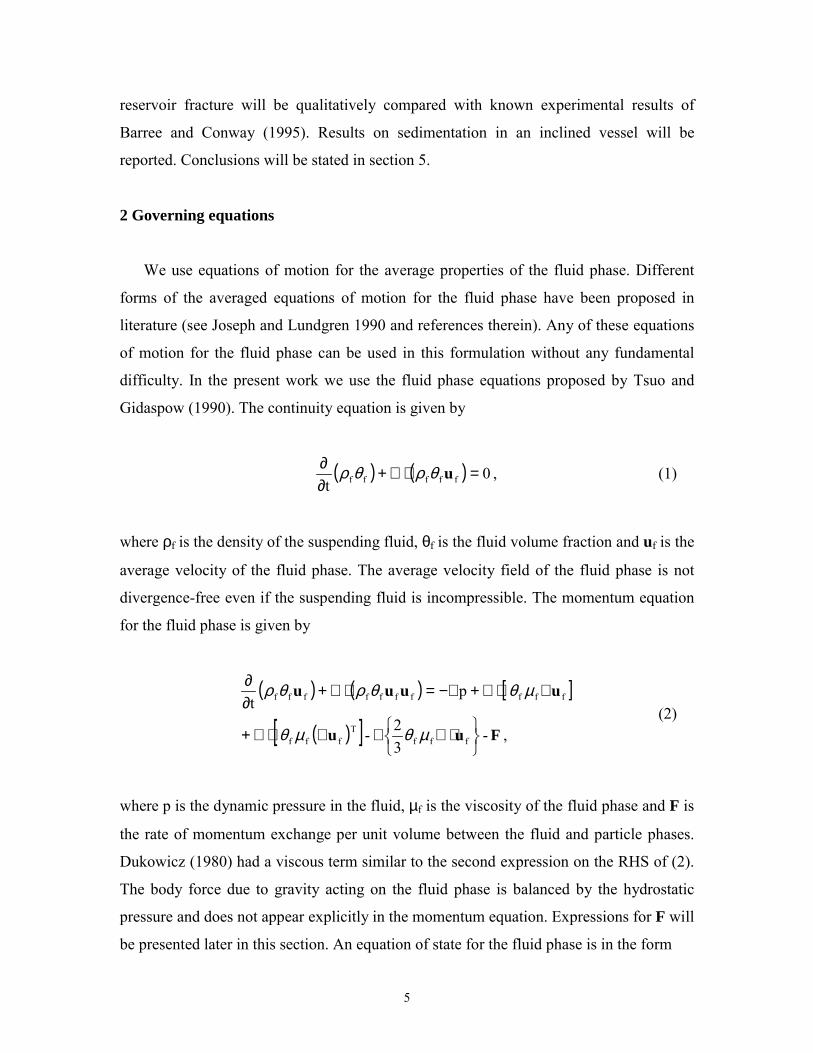
2 Governing equations

We use equations of motion for the average properties of the fluid phase. Different

forms of the averaged equations of motion for the fluid phase have been proposed in

literature (see Joseph and Lundgren 1990 and references therein). Any of these equations

of motion for the fluid phase can be used in this formulation without any fundamental

difficulty. In the present work we use the fluid phase equations proposed by Tsuo and

Gidaspow (1990). The continuity equation is given by

( ) ( ) , 0t fffff =⋅∇+

∂∂ uθρθρ (1)

where ρf is the density of the suspending fluid, θf is the fluid volume fraction and uf is the

average velocity of the fluid phase. The average velocity field of the fluid phase is not

divergence-free even if the suspending fluid is incompressible. The momentum equation

for the fluid phase is given by

( ) ( ) [ ]

( )[ ] , -32-

pt

fffT

fff

ffffffffff

Fuu

uuuu

���

��� ⋅∇∇∇⋅∇+

∇⋅∇+−∇=⋅∇+∂∂

µθµθ

µθθρθρ(2)

where p is the dynamic pressure in the fluid, µf is the viscosity of the fluid phase and F is

the rate of momentum exchange per unit volume between the fluid and particle phases.

Dukowicz (1980) had a viscous term similar to the second expression on the RHS of (2).

The body force due to gravity acting on the fluid phase is balanced by the hydrostatic

pressure and does not appear explicitly in the momentum equation. Expressions for F will

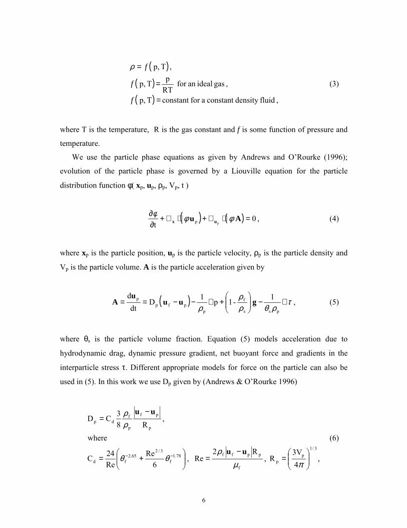
be presented later in this section. An equation of state for the fluid phase is in the form

6

( )( )( ) , fluiddensity constant afor constant T p,

, gas idealan for RTp T p,

, T p,

=

=

=

f

f

fρ

(3)

where T is the temperature, R is the gas constant and f is some function of pressure and

temperature.

We use the particle phase equations as given by Andrews and O’Rourke (1996);

evolution of the particle phase is governed by a Liouville equation for the particle

distribution function φ( xp, up, ρp, Vp, t )

( ) ( ) , 0 t pp =⋅∇+⋅∇+

∂∂ Au ux φφφ (4)

where xp is the particle position, up is the particle velocity, ρp is the particle density and

Vp is the particle volume. A is the particle acceleration given by

( ) , 1 -1p1 Ddt

d

pss

f

ppfp

p τρθρ

ρρ

∇−���

����

�+∇−−== guu

uA (5)

where θs is the particle volume fraction. Equation (5) models acceleration due to

hydrodynamic drag, dynamic pressure gradient, net buoyant force and gradients in the

interparticle stress τ. Different appropriate models for force on the particle can also be

used in (5). In this work we use Dp given by (Andrews & O’Rourke 1996)

,43V

R , R2

Re , 6

ReRe24C

where

, R8

3CD

3/1p

pf

ppff78.1f

3/265.2

fd

p

pf

p

fdp

���

����

�=

−=��

�

����

�+=

−=

−−

πµρ

θθ

ρρ

uu

uu

(6)

7

Cd is the drag coefficient, Re is the Reynolds number and Rp is the particle radius (we

assume spherical particles). Particle-particle collisions are modeled by an isotropic

interparticle stress given by (Harris and Crighton 1994)

scs

ssPθθ

θτβ

−= , (7)

where Ps has units of pressure, θcs is the particle volume fraction at close packing and β is

a constant. A discussion of the factors entering into the choice of Ps and β is given by

Snider et al. (1998). In (7) it is assumed that acceleration of a particle due to interparticle

stress is independent of its size and velocity. Any stress model that accounts for the effect

of particle size and velocity can replace (7) when available. The particle volume fraction

θs is defined by

���= pppps dddVV uρφθ . (8)

Fluid volume fraction θf is then given by

sf 1 θθ −= . (9)

The interphase momentum transfer function F is given by

( )������

�

���

�∇−−= ppp

ppfppp dddVp1DV uuuF ρ

ρρφ . (10)

Andrews and O’Rourke (1996) highlighted several important features of this formulation.

The previous Eulerian/ Lagrangian formulations (e.g. Dukowicz 1980) ignored the

interparticle stress term which is modeled in the present approach. It can be shown by

deriving the average momentum equation for particle phase from (4) that this formulation

8

accounts for the kinematic stress that arises from local particle velocity fluctuations about

the mean velocity. The effect of buoyancy driven currents is modeled in this formulation.

This can be verified by adding the average momentum equations for the fluid and particle

phases. This is also confirmed by our numerical simulation of the Rayleigh-Taylor

instability (to be presented later) during the sedimentation of particles initially placed at

the top in a sedimentation column.

3 Numerical scheme

We use a finite-volume method on an Eulerian grid to solve the fluid phase equations

in cartesian coordinate system. A non-staggered grid for velocity and pressure (Rhie and

Chow 1982) is used. The particle phase equations are solved by considering the motion

of a finite number of computational particles which represent a sample of the total

population of particles. Each computational particle, henceforth referred to as a parcel, is

considered to represent a group of particles of identical size, velocity and position.

3.1 Interpolation scheme

In order solve the particle equation of motion it is necessary to interpolate variables to

the particle position. Similarly the solution of fluid phase equations requires the

calculation of variables on the Eulerian grid. This requires the interpolation of these

variables from particle location to the Eulerian grid. This is accomplished by using

bilinear interpolation function formed from the product of linear interpolation functions

in the x, y and z directions (see Snider et al. 1998). The bilinear interpolation function

Sijk(x) is unity at a given grid node (i,j,k) which is at the cell center and decreases to zero

at the 26 neighboring nodes and the domain beyond these neighboring nodes. The

position xp of any particle can be located in a box defined by eight Eulerian grid nodes

surrounding it. The sum of the eight interpolation functions, due to the surrounding

nodes, at a particle location is unity.

The particle volume fraction on the Eulerian grid is calculated by

9

( )�=p

pijkppijk

sijk SVNV1 xθ , (11)

where θsijk is the particle volume fraction at grid node (i,j,k), Vijk is the volume of the

Eulerian cell (i,j,k) and Np is the number of particles in a parcel. The fluid volume

fraction θfijk at grid node (i,j,k) immediately follows from (9).

An example of the interpolation of a variable from the grid node to particle position is

given by

( )�=

=8

1fpfp S

ςςς uxu , (12)

where ufp is the fluid velocity at the particle location and ζ is an index for the eight grid

nodes bounding the particle.

The interphase momentum transfer Fijk at a grid node (i,j,k) is evaluated by an

interpolation scheme given by Snider et al. 1998. According to this scheme the

expression for Fijk is given by

( ) ( )

( ) ( )�

�

��

���

��

���

��

���

∇−−=

��

���

��

���

��

���

∇−−=

pijk

ppfijkppijkppp

ijk

pp

ppfpppijkppp

ijkijk

p1D SNVV1

p1D SNVV1

ρρ

ρρ

uux

uuxF

(13)

This gives a less diffusive interpolation scheme and increases the diagonal dominance of

the momentum equation of the fluid phase.

3.2 Numerical algorithm

We use an explicit update of the particle positions in which the translational motion

of the particles is solved based on the fluid velocity and pressure fields at the end of the

10

previous time step. Motion of each particle type represents the motion of the parcel it

represents. In our numerical algorithm we first solve for the particle equations of motion.

This is followed by a solution of the fluid phase equations. The fluid properties ρf and µf

are constant.

3.2.1 Numerical scheme for particle motion

Given the solution at the end of n time-steps i.e. given npu , n

px for particles in all the

parcels, nnf p and u , compute 1n

p+u and 1n

p+x by the following procedure:

For particles in all the parcels:

Set np

n,0p

np

n,0p , xxuu == .

do k=1,K

( )1-kn,p

ps

kn,*pp

p

fn

p

nfp1

11-kn,

pkn,*

p

at 1D

1p1D

where, K

t

xu

guf

fuu

��

���

∇−−

��

���

��

���

��

�

�

��

�

�−+∇−=

∆+=

τρθ

ρρ

ρ(14)

��

�

�

��

�

� +∆+=2K

t k*n,p

1-kn,p1-kn,

pkn,*

p

uuxx (15)

( )kn,*p

ps

kn,pp

p

fn

p

nfp2

211-kn,p

kn,p

at 1D

1p1D

where, 2K

t

xu

guf

ffuu

��

���

∇−−

��

���

��

���

��

�

�

��

�

�−+∇−=

��

���

� +∆+=

τρθ

ρρ

ρ(16)

11

��

�

�

��

�

� +∆+=2K

t kn,p

1-kn,p1-kn,

pkn,

p

uuxx (17)

enddo

Set Kn,p

1np

Kn,p

1np , xxuu == ++ . Calculate 1n

s+θ by using (11).

Here, ∆t is the time-step. In this step the effective time-step for the motion of particles is

reduced if the value of K is greater than one. This is helpful to avoid instability due to the

interparticle stress term. In our numerical simulations K varies between 2 to 5. Value

smaller than 2 led to instabilities. The choice of K depends on the application and is

usually set ad hoc based on numerical trials. Eventually a systematic choice of K is

desirable and is under investigation. Note that the original MP-PIC approach used an

implicit scheme to avoid using small time steps. A similar scheme was used by

Glowinski, Pan, Hesla and Joseph (1999) to solve for the motion of particles in their

direct numerical simulation method for fluid-particle mixtures. Near the close packing

limit we use a large but finite value for the particle stress. Our scheme is not completely

robust near the close packing limit although we did simulate some challenging problems

e.g. see fig. 4-7. Improvement of our scheme in this regard is the subject of our current

investigation.

3.2.2 Numerical scheme for fluid phase equations

We use a non-staggered cartesian grid to solve the fluid phase equations (Rhie and

Chow 1982). The pressure and the cartesian velocity components are defined at the center

of the control volume. Mass fluxes are defined at the mid-point of their corresponding

faces of the control volume. We use a Chorin-type fractional-step method (Chorin 1968)

based on a pressure correction scheme. This pressure correction based scheme has several

features similar to the SIMPLE approach of Patankar and Spalding (1972). A fractional-

step based pressure correction scheme for the turbulent flow of a Newtonian fluid was

12

presented by Comini and Del Giudice (1985). A variation of the fractional-step pressure

correction approach was also presented by Choi, Choi and Yoo (1996). The fluid phase

equations are solved by the following solution procedure:

(1) Given nnf p ,u , n

sθ , 1ns

+θ , 1np

+u and 1np

+x , compute the intermediate velocity *fu at the

grid nodes by solving:

( ) ( ) ( ) ( )

( )[ ] ,ijk node grid , D SNVV1p

tPD

t

p

1npp

1npijkppp

ijk

n1np

f1n

fnff

1nf

nf

nf

nffn*

f*ff

*f

1nff

∀+∇+

∇⋅∇−∇⋅∇+

∆+−∇=ℑ++

∆

�+++

++

+

ux

uu

uuuu

ρθ

µθµθ

θρθρ

(18)

where P is defined by

fff31-pP u⋅∇= µθ . (19)

and

( )[ ] ijk. node gridany for , D SNVV1D

pp

1npijkppp

ijkf �

+= xρ (20)

ℑ is the convection-diffusion operator whose operation on any vector v is given by

( ){ }vuv f1

fnf

1ff ∇−⋅∇=ℑ ++ µθθρ nn . (21)

Time discretization of (2) and appropriate rearrangement of the terms results in (18). A

‘half implicit’ expression, ( )1nf

nf

1nff

++⋅∇ uuθρ , is used for the convection term. This

expression is first-order accurate. Fluid phase velocity nfu in the convection term can be

13

replaced by a second-order accurate expression given by 1-nf

nf2 uu − (Turek 1996). We

can employ approximate factorization technique (Beam and Warming 1976, Briley and

McDonald 1977) in which (18) is factorized as

( )

( )

( ) ( ) ( ) ( )

( )[ ] ,ijk node grid , D SNVV1p

D t

P

C

t1C

t1C

t1t

C

p

1npp

1npijkppp

ijk

n1np

f1n

fnff

1nf

nf

nf

nff

1nf

nf

nffn

nf

*fz

uy

ux

u

u

∀+∇+

∇⋅∇−∇⋅∇+

ℑ−−−∆

+∇−

=−��

���

�ℑ∆+�

�

���

�ℑ∆+�

�

���

�ℑ∆+�

�

�

�

∆

�+++

++

+

ux

uu

uuu

uu

ρθ

µθµθ

θθρ

(22)

where

. z

uz

, y

uy

, x

ux

,t DC

f1n

fn

z f1n

ffz

f1n

fn

y f1n

ffy

f1n

fn xf

1nffx

f1n

ffu

���

���

��

�

�

∂∂−

∂∂=ℑ

���

���

���

�

�

∂∂−

∂∂=ℑ

���

���

��

�

�

∂∂−

∂∂=ℑ

∆+=

++

++

++

+

vv

vv

vv

µθθρ

µθθρ

µθθρ

θρ

(23)

It can be easily shown that the error in this factorization is O(∆t3). An approximate

factorization technique in conjunction with fractional-step method to simulate turbulent

flows was developed by Kim and Moin (1985).

We can solve either (18) or (22) during our simulations. Both approaches are first-

order with respect of temporal discretization and gave similar results. Solving (18) does

not involve the additional error of factorization whereas using (22) offers a faster solution

procedure. We use the power-law upwinding scheme (Patankar 1980) for this convection-

14

diffusion problem giving a first-order discretization in computational space. Boundary

values of the intermediate velocity are the same as the velocity specified at the boundary.

This is permissible for a first-order pressure correction based scheme where (26) (the

velocity correction equation to be presented later) shows that the resulting error is O(∆t2)

(Choi, Choi and Yoo 1997). The solution of (18) is obtained by a block-correction-based

multigrid method (Sathyamurthy and Patankar 1994). This method employs a multilevel

correction strategy and is based on the principle of deriving the coarse grid discretization

equations from the fine grid discretization equations. The solution of (22) is non-iterative

and faster involving solution of three tridiagonal matrices.

(2) Given *fu at the grid nodes, compute the intermediate velocity ( )cf

*fu on cell faces by

linear interpolation. Value of ( )cf*fu on the boundary cell faces is calculated by linear

extrapolation of the values of *fu at the interior grid nodes. Other upwind interpolation

methods such as the QUICK formulation (Leonard 1979) can be used. We consider only

linear interpolation scheme in the present work for this computational step.

(3) Given ( )cf*fu and Pn, compute Pn+1. Correction of cell face velocity is given by

( ) ( ) ,P

tcf

*f

1ffcf

1nf

1ff ′−∇=

∆− +++ uu nn θρθρ

(24)

where n1n P-PP +=′ is the pressure correction defined at grid node. The pressure

correction equation is obtained by using (24) in the continuity equation (1). The discrete

form of the equation is then given by

( ) ( )

( )[ ] ( )[ ] ( )[ ] , uz

uy

u x

t t1P

z z P

y y P

x x

cf*

z f1n

ffcf*

y f1n

ffcf* xf

1nff

nff

1nff

���

+++

���

∆−

∆=�

�

�

� ′+���

�

� ′+��

�

� ′

+++

+

θρδδθρ

δδθρ

δδ

θρθρδδ

δδ

δδ

δδ

δδ

δδ

(25)

15

where δ/δx, δ/δy and δ/δz represent discrete difference operators in the computational

space. We use the velocity specified at the boundary while setting up the pressure

correction equation (25). Thus pressure correction at the boundary does not appear in (25)

(Patankar 1980). We therefore do not need a boundary condition for pressure correction

to solve (25). We use the block-correction-based multigrid method (Sathyamurthy and

Patankar 1994) to solve (25). To obtain pressure correction at the boundary we apply (24)

at the boundary cell faces where both ( )cf1n

f+u and ( )cf

*fu are known. Pn+1 follows directly

from the solution for P′ . Velocities at the internal cell faces at the end of the present

time-step are computed using (24). These cell face velocities are used to calculate the

mass flux in the ‘half implicit’ convection term in the next time step.

(4) Given P′ , compute 1nf

+u and pn+1. The velocity at grid nodes is corrected by

( ) ( ) ,P

t

*f

1ff

1nf

1ff ′−∇=

∆− +++ uu nn θρθρ

(26)

where the gradient of pressure correction at the grid node is calculated by a central

difference scheme. The pressure pn+1 then follows from (19). The value of pressure in the

domain is calculated with respect to the value at some reference point inside the

computational space. Convergence is said to be achieved if the residue is less than 10-10.

4 Numerical results

We validate the numerical scheme by comparing calculated sedimentation rates with

the values measured in the experiments of Davis, Herbolzheimer and Acrivos (1982) for

a bimodal suspension. The sedimentation column in the experiment was vertical, 100 cm

tall and has a square cross-section with each side 5 cm wide. The calculation domain in

our simulations have x, y and z dimensions equal to 5 cm, 125 cm and 5 cm, respectively.

Gravity acts in the negative y-direction. The suspending fluid is Newtonian with the

density and viscosity being 992 kg/m3 and 0.0667 kg/(m-s), respectively. Particles of two

16

different densities are used in the calculations. The density of the heavy particles is 2990

kg/m3; their diameters vary uniformly between 177 µm to 219 µm. The density of lighter

particles is 2440 kg/m3 and their diameters range uniformly between 125 µm to 150 µm.

The initial concentration of the heavy particles is 0.01 and that of lighter particles is 0.03.

The particles are initially placed randomly with uniform distribution upto a height of 100

cm of the sedimentation column. To model the interparticle stress we choose Ps = 100 Pa,

β = 3 and θcs = 0.6.

In order to check the convergence of the numerical scheme we perform two

simulations with different grid size, number of parcels and time steps. In Case A there are

10 control volumes in the x and z directions and 50 control volumes in the y direction.

There are 9000 parcels of each type giving a total of 18000 parcels. The number of

particles in each parcel is chosen so that the total particle volume in each parcel is the

same for heavy and light parcel types, respectively. The time step is 0.05 s. To start the

simulation from rest we use smaller time steps beginning from 0.00078125 s and

increasing every subsequent time step by a factor of two until it becomes 0.05 s. For Case

B we double the number of control volumes and parcels in the domain. The time step is

reduced by half. Here we present convergence results for the numerical scheme based on

the solution procedure without approximate factorization. Similar convergence tests were

also performed for the method of approximate factorization and are not reported here.

Figure 1 shows the transient interface levels of the two types of particles. Here the

comparison is made between the LNS calculations from Cases A and B and the

experimental data of Davis et al. (1982). We see that they are in good agreement thus

validating the calculations by the present numerical procedure. Figure 2 shows the parcel

positions in the channel at different times for Case B. Figure 3 shows the particle

positions at t = 300 s calculated from Cases A and B. We see that they have almost

identical particle distributions. The coarse mesh simulation required around 4 MB

memory and took less than 8 s CPU time for completing one time step on a SGI machine.

We now apply the scheme to the sedimentation of particles initially placed at the top

in a sedimentation column. This is similar to the presence of heavy fluid on top of a light

fluid. Such a configuration should then give rise to a Rayleigh-Taylor instability. This

instability was indeed reproduced in the direct numerical simulation of particles falling a

17

Newtonian fluid by Glowinski et al. (1999). To ensure that our numerical scheme is able

to capture such instabilities we simulated this case. The x, y and z dimensions of the

sedimentation column are 10 cm, 50 cm and 5 cm, respectively. Gravity acts in the

negative y-direction. The density and viscosity of the Newtonian suspending fluid are

1000 kg/m3 and 0.00667 kg/(m-s), respectively. The particle density is 2500 kg/m3 and

the diameter is 126 µm. Particles are initially placed in the top half of the sedimentation

column in a regular array and their volume fraction is 0.1. We use the same parameters as

before to model the interparticle stress. There are 17280 parcels in the calculation domain

with each parcel having 6910 particles. There are 10 control volumes in the x-direction,

40 in the y-direction and 5 in the z-direction. The time step after the initial transient is

0.05 s.

Figure 4 shows the particle positions in the sedimentation column at different times.

Figure 5 shows the three-dimensional view at t = 17.5 s. It is seen that a Rayleigh-Taylor

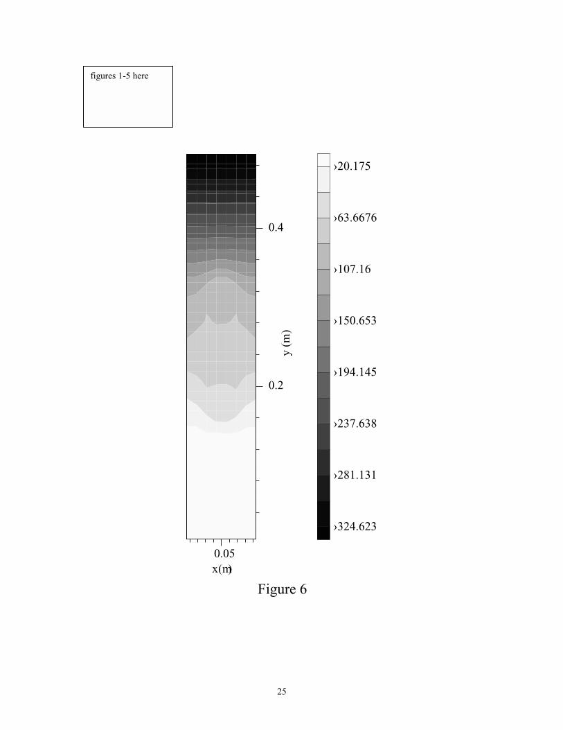
instability develops leading to particles falling faster near the walls (Figure 4a). Particles

near the axis of the channel are retarded due to an adverse pressure gradient acting on

them (Figure 6). The falling particles further ‘pull’ the particles from the top. This motion

eventually leads to the entrainment of fluid in the fluid-particle suspension (Figure 4b).

The ‘bubble’ of fluid rises and breaks open at the top of the column leading to the

ejection of particles (Figure 4b, Figure 5 and Figure 4c). This also leads to the formation

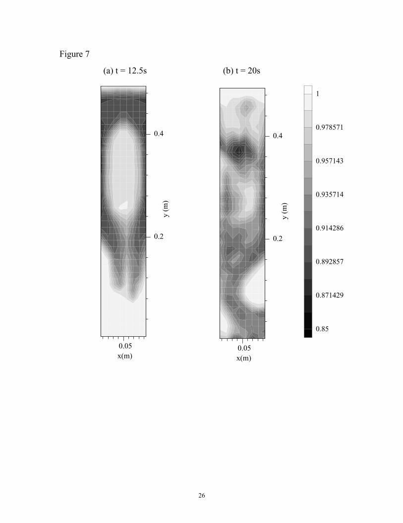
of local particle clusters (Figure 4d and Figure 7b). The particles eventually begin to

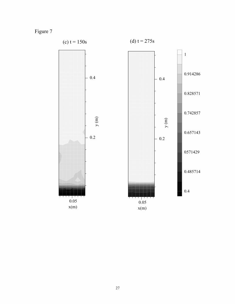
settle steadily to the bottom of the column to a no-motion state. Figure 7 shows the fluid

concentration at different times in the x-y plane and averaged with respect to the z-

direction. In the final no-motion state (Figure 7d) the extra weight of the particles is

balanced by the interparticle stress.

The present scheme is used to simulate the flow of solid-liquid mixtures in fractured

reservoirs. Barree and Conway (1995) reported experimental and numerical study of

convective proppant transport. We consider the flow of solid-liquid mixture in a channel

or slot that is 7.5 m long (x-direction), 25 cm high (y-direction) and 6.3 mm wide (z-

direction). Gravity acts in the negative y-direction. We have 150 control volumes in the

x-direction, 10 control volumes in the y-direction and 5 control volumes in the z-

direction. The fluid and particle properties and the parameters for interparticle stress

18

model are the same as that used in the simulation of the sedimentation column. There are

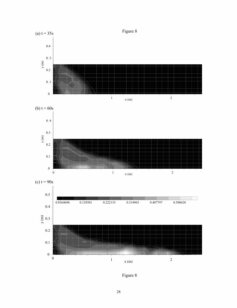
initially no particles in the channel. We simulate two cases. Figure 8 shows the particle

concentration at different times in the x-y plane and averaged with respect to the z-

direction for the first case. In this case the fluid-particle mixture is introduced uniformly,

at a volumetric flow rate of 19.69 cm3/s and particle concentration of 10%, from the top

half of the channel at the left end. It is seen that a gravity tongue develops which is

identical to the one seen in the experiments of Barree and Conway (1995). The particles

continue to fall, impinge on the bottom and flow with an increased rate of lateral

transport at the bottom of the channel. This is in agreement with the experimental

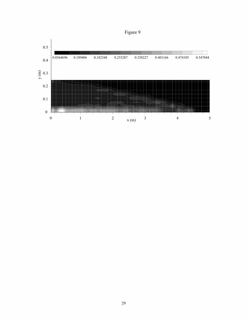
observation. In the second case the fluid-particle mixture is introduced uniformly at the

left end of the channel at a volumetric flow rate of 78.75 cm3/s and 10% particle

concentration. Once again we see formation of the gravity tongue that traverses along the

channel length (Figure 9). It is known from experiments (Kern, Perkins and Wyant 1959)

that, in such flows, particles settle and form a bed at the channel bottom. It is seen in

Figure 9 that a bed of particles is beginning to form. In these simulations there were

around 200,000 parcels in the computational domain.

We perform inclined sedimentation calculations using our numerical scheme. Acrivos

and Herbolzheimer (1979) performed experiments to calculate the sedimentation rates in

inclined columns. Experiments were run with the container tilted at different angles.

Following Snider et al. (1998) we perform calculations in a two-dimensional domain.

Our code for three-dimensional domains is used to perform calculations in two-

dimensions. The calculation domain in our simulations have x and y dimensions equal to

5 cm and 60 cm, respectively. There are 32 control volumes in the x-direction and 72

control volumes in the y-direction. Gravity acts at an angle of 35o with the negative y-

direction. Suspending fluid properties are the same as bimodal sedimentation. Density of

the particles is 2420 kg/m3; their diameters vary uniformly between 130 µm to 142 µm.

Initial concentration of the particles is 0.1. Initially, the particles are randomly placed

with uniform distribution upto a height of 52.33 cm along the y-axis (the mixture-fluid

interface is tilted at an angle to vessel walls). We use Model A for interparticle collision

with the same parameters as before. There are 18111 parcels in the calculation domain.

19

The number of particles in each parcel is chosen so that the total particle volume in each

parcel is the same. The time step is same as in bimodal simulations.

Figure 10 compares the transient interface levels of the particles from experiment

(Acrivos and Herbolzheimer 1979) and simulation. Figure 11 shows the particle positions

at different times.

The mixture-fluid interface can form wave instabilities similar to those of a fluid

flowing down an inclined plane. Herbolzheimer (1983) presented photographs of waves

at the interface in inclined sedimentation. Snider et al. (1998) simulated wave instability

at the interface. We perform the same simulation as Snider et al. (1998) and reproduce

the wave observed by them in their simulations. Fluid viscosity is changed to 0.0188 Pa-

s, particle diameter is 132 µm and particle density is 2440 kg/m3. Column inclination is

20o. Particles are filled in the column upto a height of 40 cm. All other parameters are the

same as the inclined sedimentation simulations above. Figure 12 shows the formation of

wave on the mixture-fluid interface similar to that reported by Snider et al. (1998).

Animations of some simulations reported here and some other simulations can be

seen at our web site http://www.aem.umn.edu/Solid-Liquid_Flows.

5 Conclusion

In this paper we have described an Eulerian-Lagrangian numerical simulation (LNS)

scheme for the flow of particulate mixtures. We have implemented an efficient three-

dimensional time dependent finite volume algorithm. A Chorin-type pressure-correction

based fractional-step scheme was used to solve the fluid phase equations on a non-

staggered cartesian grid. The reported scheme can account for suspending fluids with

non-constant properties.

The numerical scheme was tested through convergence tests for the bimodal

sedimentation of particles in a vessel. Results on the Rayleigh-Taylor instability of

particles sedimenting in a fluid from a height were presented. They were in good

agreement with the direct numerical simulation results reported in literature. Calculations

were done for inclined sedimentation in a vessel. Wave instability on the fluid-mixture

interface during inclined sedimentation was observed. We also simulated the flow of

20

particulate mixture in a fracture. The calculated results were in good qualitative

agreement with the experimental observations.

In summary, we present a numerical scheme that extends the MP-PIC method in the

following way (even if the viscous terms in the fluid phase equations are to be neglected):

(a) A fractional step algorithm for fluid-particle equations and (b) collocated grid for

pressure and velocity.

The numerical scheme is not limited to the particular model used for viscous stress

terms in the fluid phase. It has the flexibility to use different models for these terms. The

primary objective behind adding a viscous stress term was to provide a numerical

framework that has the flexibility to incorporate different models for various applications.

The way models are tested is through comparisons with experiments. Every model must

pass this test. If the prediction of a model disagrees with experiments then it is not valid.

If the predictions agree with few experiments it doesn’t mean that it is valid either. Our

model with viscous terms agree qualitatively with some experiments; so we are

encouraged to look further.

Acknowledgments

We acknowledge the support from NSF under KDI/NCC grant NSF/CTS-9873236 and

STIM-LAB.

References

Acrivos, A. & Herbolzheimer, E. 1979 Enhanced sedimentation in settling tanks with

inclined walls. J. Fluid Mech. 92, 435-457.

Andrews, M. J. & O’Rourke, P. J. 1996 The multiphase particle-in-cell (MP-PIC) method

for dense particulate flows. Int. J. Multiphase Flow 22, 379-402.

Barree, R. D. & Conway, M. W. 1995 Experimental and numerical modeling of

convective proppant transport. J. Petroleum Tech. 47, 216-222.

Batchelor, G. K. 1988 A new theory of the instability of a uniform fluidized bed. J. Fluid

Mech. 193, 75-110.

21

Beam, R. M. & Warming, R. F. 1976 An implicit finite-difference algorithm for

hyperbolic systems in conservation-law form. J. Comput. Phys. 22, 87-110.

Briley, W. R. & McDonald, H. 1977 Solution of the multidimensional compressible

Navier-Stokes equations by a generalized implicit method. J. Comput. Phys. 24, 372-

397.

Choi, H. G., Choi, H. & Yoo, J. Y. 1997 A fractional four-step finite element formulation

of the unsteady incompressible Navier-Stokes equations using SUPG and linear

equal-order element methods. Comput. Methods Appl. Mech. Engrg. 113, 333-348.

Chorin, A. J. 1968 Numerical solution of the Navier-Stokes equations. Math. Comput. 22,

745-762.

Comini, G. & Del Giudice S. 1985 A (k-ε) model of turbulent flow. Numer. Heat

Transfer 8, 133-147.

Crowe, C. T., Sharma, M. P. & Stock, D. E. 1977 The particle-source-in cell (PSI-CELL)

model for gas-droplet flows. Trans. ASME J. Fluids Engrg. 99, 325-332.

Davis, R. H., Herbolzheimer, E. & Acrivos, A. 1982 The sedimentation of polydisperse

suspensions in vessels having inclined walls. Int. J. Multiphase Flow 8, 571-585.

Dukowicz, J. K. 1980 A particle-fluid numerical model for liquid sprays. J. Comput.

Phys. 35, 229-253.

Gauvin, W. H., Katta, S. & Knelman, F. H. 1975 Drop trajectory predictions and their

importance in the design of spray dryers. Int. J. Multiphase Flow 1, 793-816.

Gidaspow, D. 1994 Multiphase Flow and Fluidization Continuum and Kinetic Theory

Descriptions. Academic Press, Boston, MA.

Glowinski, R., Pan, T.-W., Hesla, T. I. & Joseph, D. D. 1999 A distributed Lagrange

multiplier/fictitious domain method for particulate flows. Int. J.Multiphase Flow, to

appear.

Harris, S. E. & Crighton, D. G. 1994 Solitons, solitary waves and voidage disturbances in

gas-fluidized beds. J. Fluid Mech. 266, 243-276.

Herbolzheimer, E. 1983 Stability of the flow during sedimentation in inclined channels.

Phys. Fluids 26, 2043-2045.

Hu, H. H. 1996 Direct simulation of flows of solid-liquid mixtures. Int. J. Multiphase

Flow 22, 335-352.

22

Hu, H. H., Joseph, D. D. & Crochet, M. J. 1992 Direct numerical simulation of fluid

particle motions. Theoret. Comput. Fluid Dynamics. 3, 285-306.

Johnson, A. & Tezduyar, T. 1997 Fluid-particle simulations reaching 100 particles.

Research report 97-010, Army High Performance Computing Research Center,

University of Minnesota.

Joseph, D. D. & Lundgren, T. S. 1990 Ensemble averaged and mixture theory equations

for incompressible fluid-particle suspensions. Int. J. Multiphase Flow 16, 35-42.

Kern, L. R., Perkins, T. K. & Wyant, R. E. 1959 The mechanics of sand movement in

fracturing. Pet. Trans. AIME 216, 403-405.

Kim, J. & Moin, P. 1985 Application of a fractional-step method to incompressible

Navier-Stokes equations. J. Comput. Phys. 59, 308-323.

Leonard, B. P. 1979 A stable and accurate convective modeling procedure based on

quadratic upstream interpolation. Comput. Methods Appl. Mech. Engrg. 19, 59-98.

Patankar, N. A., Singh, P., Joseph, D. D., Glowinski, R. & Pan, T.-W. 1999 A new

formulation of the distributed Lagrange multiplier/fictitious domain method for

particulate flows. Int. J. Multiphase Flow, to appear.

Patankar, S. V. 1980 Numerical Heat Transfer and Fluid Flow. Hemisphere Publishing

Corporation, New York, NY.

Patankar, S. V. & Spalding, D. B. 1972 A calculation procedure for heat, mass and

momentum transfer in three-dimensional parabolic flows. Int. J. Heat Mass Transfer

15, 1787-1806.

Perić, M., Kessler, R. & Scheuerer, G. 1988 Comparison of finite-volume numerical

methods with staggered and colocated grids. Comput. Fluids 16, 389-403.

Rhie, C. M. & Chow, W. L. 1982 A numerical study of the turbulent flow past an isolated

airfoil with trailing edge separation. AIAA-82-0998.

Sathyamurthy, P. S. & Patankar, S. V. 1994 Block-correction-based multigrid method for

fluid flow problems. Numer. Heat Transfer, Part B 25, 375-394.

Snider, D. M., O’Rourke, P. J. & Andrews, M. J. 1998 Sediment flow in inclined vessels

calculated using a multiphase particle-in-cell model for dense particle flows. Int. J.

Multiphase Flow 24, 1359-1382.

23

Tsuo, Y. P. & Gidaspow, D. 1990 Computation of flow patterns in circulating fluidized

beds. AIChE J. 36, 885-896.

Turek, S. 1996 A comparative study of time-stepping techniques for the incompressible

Navier-Stokes equations: from fully implicit non-linear schemes to semi-implicit

projection methods. Int. J. Numer. Methods Fluids 22, 987-1011.

Williams, F. A. 1985 Combustion Theory, 2nd Edn. Benjamin/Cummings, Menlo Park,

CA.

Zhang, Y., Street, R. L. & Koseff, J. R. 1994 A non-staggered grid, fractional step

method for time-dependent incompressible Navier-Stokes equations in curvilinear

coordinates. J. Comput. Phys. 114, 18-33.

24

Figure Captions

Figure 1. Transient interface levels for bimodal batch sedimentation of particles.

Figure 2. Calculated (Case B) parcel positions at different times for bimodal batch

sedimentation of particles.

Figure 3. Comparison of parcel positions in bimodal batch sedimentation for Cases A and

B at t = 300s.

Figure 4. Parcel positions at different times depicting the Rayleigh-Taylor instability of

particles falling in a sedimentation column.

Figure 5. A three-dimensional view of parcel positions in a sedimentation column.

Figure 6. Contour plot for pressure averaged in the z-direction in a sedimentation column.

Figure 7. Contour plot of fluid volume fraction averaged in the z-direction at different

times in a sedimentation column. The particles are fully settled at t = 275s.

Figure 8. Contour plot of particle volume fraction averaged in the z-direction at different

times for flow of fluid-particle mixture in a fracture. Particles are introduced

uniformly at the top half of the channel entrance to the left.

Figure 9. Contour plot of particle volume fraction averaged in the z-direction at t = 79.2s

for flow of fluid-particle mixture in a fracture. Particles are introduced uniformly at

the channel entrance to the left.

Figure 10. Transient interface level during inclined sedimentation of particles.

Figure 11. Parcel positions at different times during inclined sedimentation.

Figure 12. Formation of wave at the fluid-mixture interface during inclined

sedimentation.

25

figures 1-5 here

0.2

0.4

y (

m)

0.05

x(m)

›20.175

›63.6676

›107.16

›150.653

›194.145

›237.638

›281.131

›324.623

Figure 6

26

0.2

0.4

y (

m)

0.05

x(m)

1

0.978571

0.957143

0.935714

0.914286

0.892857

0.871429

0.85

(b) t = 20s

0.2

0.4

y (

m)

0.05

x(m)

(a) t = 12.5s

Figure 7

27

0.2

0.4

y (

m)

0.05

x(m)

(c) t = 150s

Figure 7

0.2

0.4

y (

m)

0.05

x(m)

1

0.914286

0.828571

0.742857

0.657143

0.571429

0.485714

0.4

(d) t = 275s

28

x (m)

y (

m)

1 2

0

0. 1

0.2

0. 3

0.4

(a) t = 35sFigure 8

x (m)

y (

m)

0 1 2

0

0.1

0.2

0.3

0. 4

(b) t = 60s

x (m)

y (

m)

1 2

0

0.1

0.2

0.3

0.4

0.5

0.0364696 0.129301 0.222133 0.314965 0.407797 0.500628

(c) t = 90s

Figure 8

0

29

x (m)

y (

m)

1 2 3 4 5

0

0.1

0.2

0.3

0.4

0.5

0.0364696 0.109406 0.182348 0.255287 0.328227 0.401166 0.474105 0.547044

Figure 9

0