LabVIEWMathscript

LabVIEWMathscript

A LabVIEW tool for executing textual mathematical commands

– Matrix and vector based calculations (linear algebra) 

– Visualization of data in plots 

– Running scripts containing a number of commands written in a file 

– A large number of mathematical functions. MathScriptcommand are equal to MATLAB commands (some MATLAB commands may not be implemented). 

LabVIEWMathscript

MathScript can be used in two ways:

– In a MathScript node which appears as a frame inside the Block diagram of a VI (available on the Functions / Mathematics / Scripts & Formulas palette.)

– In a MathScript window as a desktop mathematical tool independent of LabVIEW

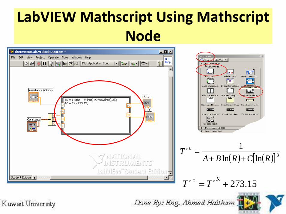
LabVIEWMathscript Using MathscriptNode

( ) ( )[ ]3lnln1

RCRBAT K

++=o

15.273+=KTT C oo

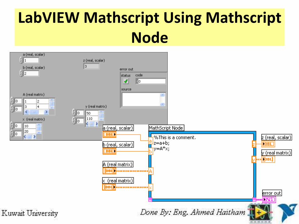
LabVIEWMathscript Using MathscriptNode

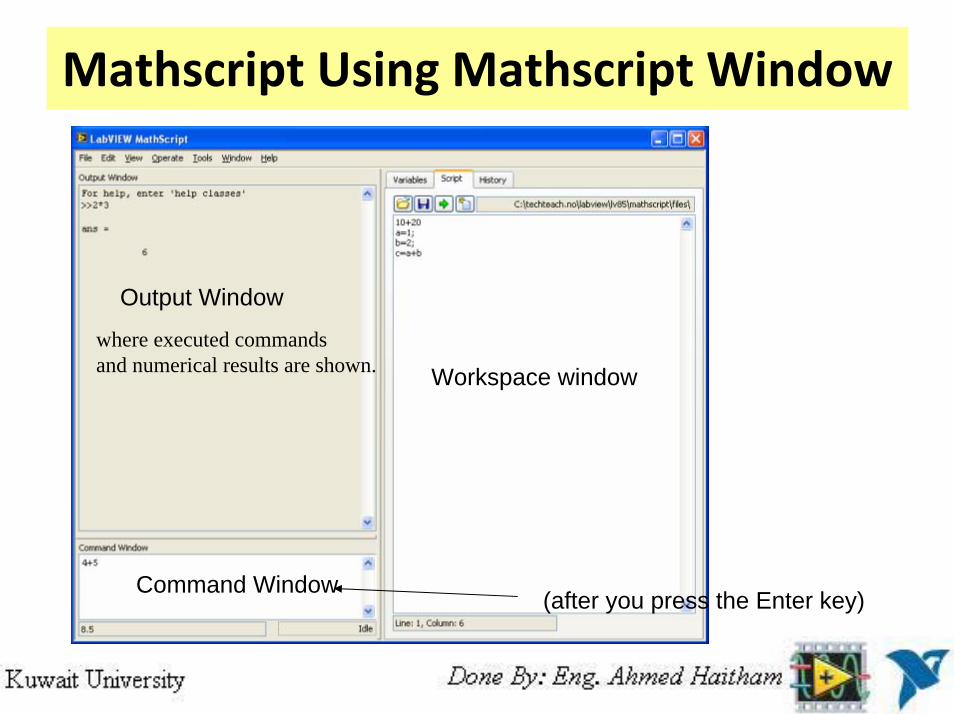
Mathscript Using Mathscript Window

Command Window

Output Window

Workspace window

(after you press the Enter key)

where executed commands and numerical results are shown.

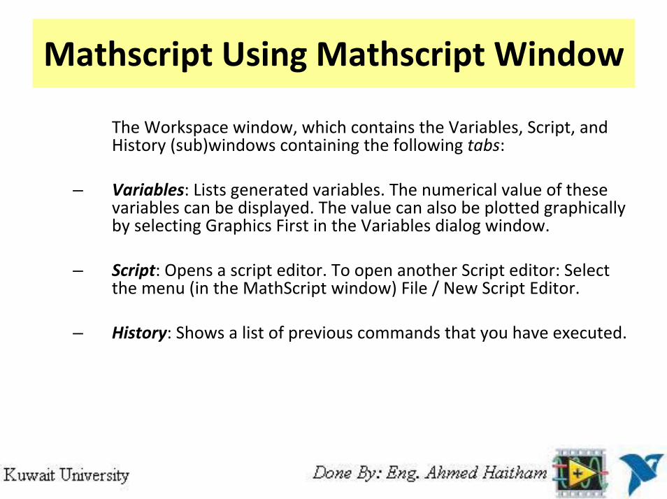
Mathscript Using Mathscript Window

The Workspace window, which contains the Variables, Script, and History (sub)windows containing the following tabs: 

– Variables: Lists generated variables. The numerical value of these variables can be displayed. The value can also be plotted graphically by selecting Graphics First in the Variables dialog window. 

– Script: Opens a script editor. To open another Script editor: Select the menu (in the MathScript window) File / New Script Editor. 

– History: Shows a list of previous commands that you have executed. 

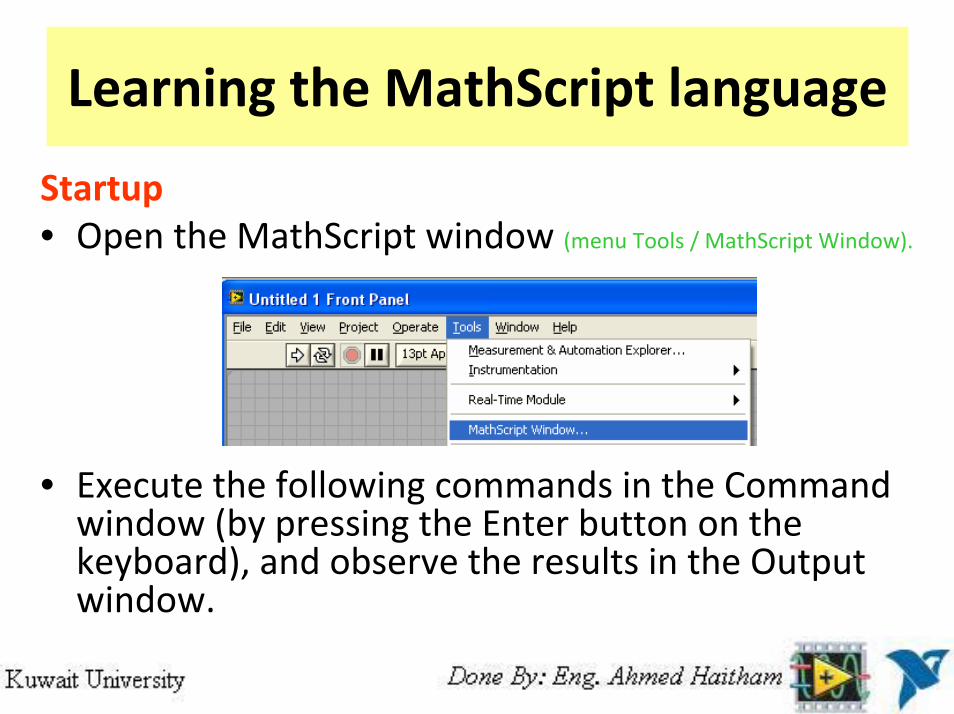
Learning the MathScript language

Startup• Open the MathScript window (menu Tools / MathScript Window).

• Execute the following commands in the Command window (by pressing the Enter button on the keyboard), and observe the results in the Output window.

Learning the MathScript language• 1+2 The result is 3 

To add 4 to ans:• ans+4 ans now gets value 7

• Several commands may be written on one line, separating the commands using either semicolon or comma. 

• With semicolon the result of the command is not displayed in the Output window, but the command is executed. 

• With comma the result is displayed.• a=5; b=7, c=a+b• With the above commands the value of a is not displayed, 

while the values of b and c are displayed

Learning the MathScript language

Recalling previous commands• To recall previous commands, press the Arrow Up button on the keyboard as many times as needed.

• To recall a previous command starting with certain characters, type these characters followed by pressing the Arrow Down button on the keyboard. Try recalling the previous command(s) beginning with the a character:

Learning the MathScript language

Case sensitivity

• MathScript is case sensitive: 

Help• Above you used the help command. It command displays information about a known command, typically including an example. Try help sin

Number Formats

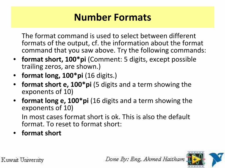
The format command is used to select between different formats of the output, cf. the information about the format command that you saw above. Try the following commands:

• format short, 100*pi (Comment: 5 digits, except possible trailing zeros, are shown.)

• format long, 100*pi (16 digits.)• format short e, 100*pi (5 digits and a term showing the 

exponents of 10)• format long e, 100*pi (16 digits and a term showing the 

exponents of 10)In most cases format short is ok. This is also the default format. To reset to format short:

• format short

Number Formats

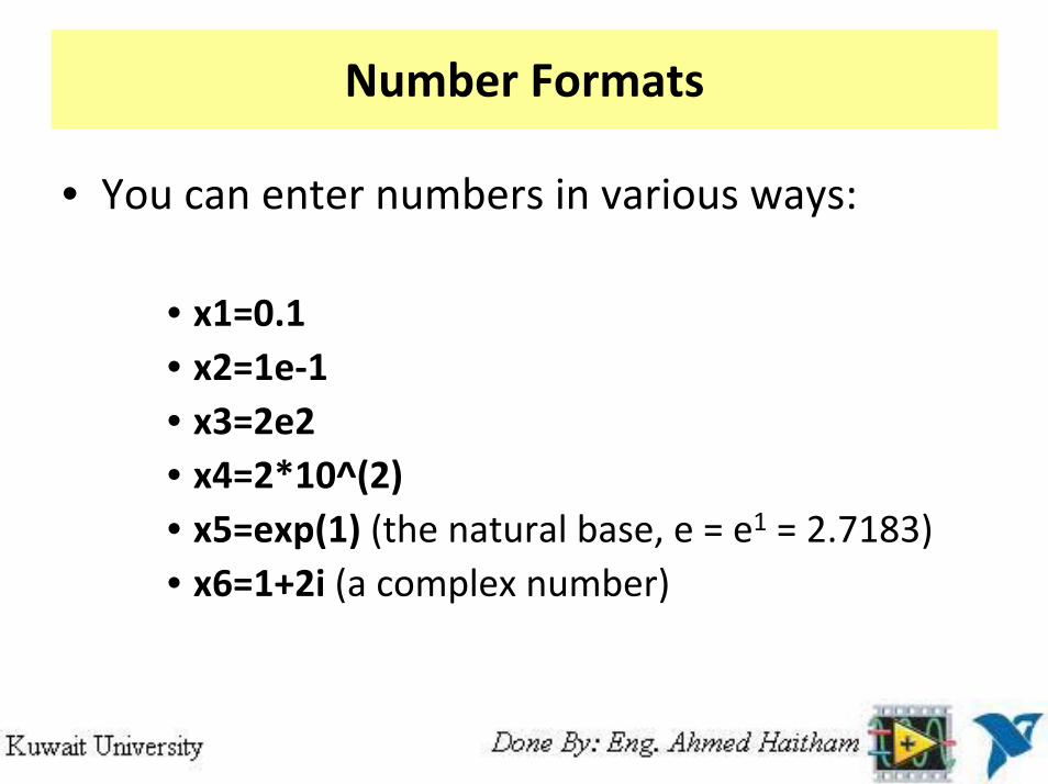
• You can enter numbers in various ways:

• x1=0.1• x2=1e‐1• x3=2e2• x4=2*10^(2)• x5=exp(1) (the natural base, e = e1 = 2.7183)• x6=1+2i (a complex number)

• All variables generated in a MathScript session (a session lasts between launching and quitting MathScript) are saved in the MathScriptWorkspace. You can see the contents of the Workspace using the menu Tools / Workspace / Variables (tab). Alternatively, you can use the who command: who

• You can delete a variable from the Workspace:clear x6

• MathScript functions are polymorphic, i.e. they typically take both scalars and vectors (arrays) as arguments. As an example, the following two commands calculate the square root of the scalar 2 and the square root of each of the elements of the vector of integers from 0 to 5, respectively:sqrt(2)sqrt([0,1,2,3,4,5])

• When the argument is a vector as in this case, the calculation is said to be vectorized.

Matrices and vectors• The matrix is the basic data element in MathScript. A matrix having only 

one row or one line are frequently denoted vector. Below are examples of creating and manipulating matrices (and vectors).

• To create a matrix, use comma to separate the elements of a row and semicolon to separate columns. For example, to create a matrix having numbers 1 and 2 in the first row and 3 and 4 in the second row:A=[1,2;3,4]

• with the resultA =

1 2 3 4 

• To transpose a matrix use the apostrophe:B=A'

• To create a row vector from say 0 to 4 with increment 1:R1=[0:4]

Matrices and vectors• To create a row vector from say 0 to 4 with increment 0.5:

R2=[0:0.5:4]• To create a column vector from say 0 to 4 with increment 1:

R3=[0:4]'• You can create matrices by combining vectors (or matrices):

C1=[1,2,3]'; C2=[4,5,6]'; M=[C1,C2]• Here are some special matrices:• You can address an element in a matrix using the standard (row number, column 

number) indexing. Note: The element indexes starts with one, not zero. (In LabVIEW, array indexes starts with zero....) For example (assuming matrix A=[1,2;3,4] is still in the Workspace), to address the (2,1) element of A and assign the value of that element to the variable w:

• w=A(2,1)with result w=3.

• You can address one whole row or column using the : (colon)operator. For example,

• C2=A(2,:)with result C2=[3,4] (displayed a little different in the Output window, though).

Element‐by‐element calculations

• Element‐by‐element calculations are executed using the dot operator together with the mathematical operator. Here is an example of calculating the product of each of the elements in two vectors:

[1,2,3].*[4,5,6]

• with result [4 10 18].

Scripts

Create a script in the Script editor (which is on the Script tab in the Workspace window (a new Script editor can opened via the menu File / New Script Editor) of name script1.m with the following contents:a=1;b=2;c=a+b

• Save the script in any folder you want.• Run the script by clicking the Run button. All the commands in the 

script are executed from top to bottom as if they were entered at the command line.

• You should make it a habit to use scripts for all your work. In this way you save your work, and you can automate your tasks.

Plotting• You can plot data using the plot command (several addition plotting 

commands are available, too). Here is an example:• Generate a vector t of assumed time values from 0 to 100 with 

increment 0.1:t=[0:.1:100]';

• Generate a vector x as a function of t:x=‐1+0.02*t;

• Generate a vector y as a function of t:y=sin(0.2*t);

• Open Figure no 1:figure(1)

• Plots x verus t, and y versus t, in the same graph:plot(t,x,t,y)

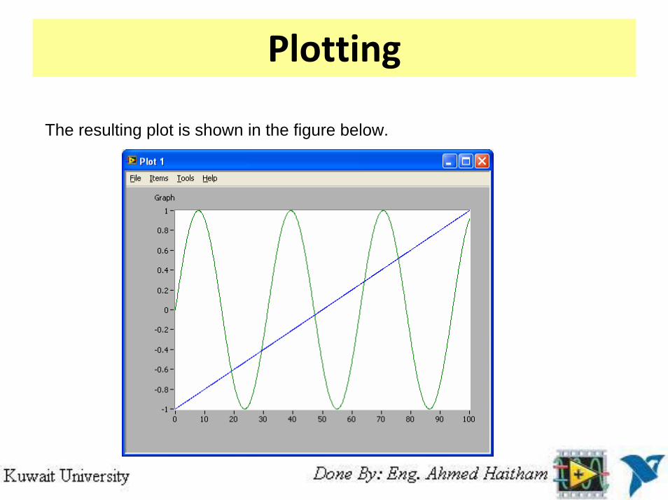
Plotting

The resulting plot is shown in the figure below.

Plotting• Probably you want to add labels, annotations, change line color etc. This can be 

done using menus in the Plot window. This is straightforward, so the options are not described here.

• As an alternative to setting labels etc. via menus in the Plot window, these can be set using commands. Below is an example, which should be self‐explaining, however note how the attributes to each curve in the plot is given, see the plot() line in the code below.t=[0:.1:100]';x=‐1+0.02*t;y=sin(0.2*t);figure(1)plot(t,x,'r‐‐',t,y,'b‐') %x(t) in dashed red. y(t) in solid blue.xmin=0;xmax=100;ymin=‐2;ymax=2;axis([xmin xmax ymin ymax])gridxlabel('t [sec]')ylabel('x (red, dashed) og y (blue, solid) [Volt]')title('Data from Experiment 1')

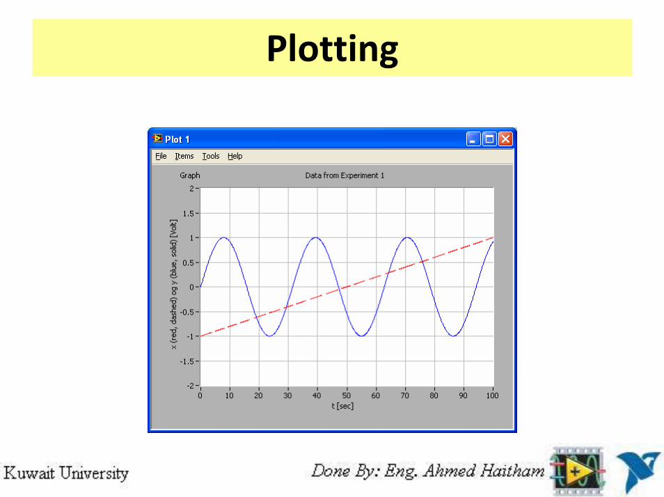
Plotting

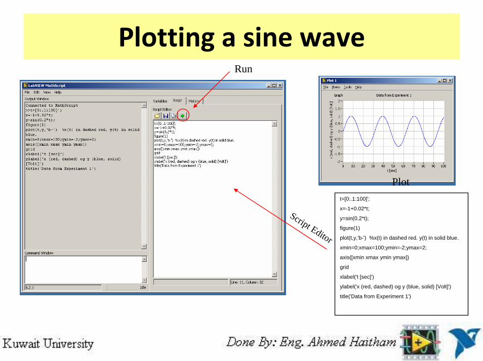
Plotting a sine wave

Script Editor

Run

Plott=[0:.1:100]';

x=-1+0.02*t;

y=sin(0.2*t);

figure(1)

plot(t,y,'b-') %x(t) in dashed red. y(t) in solid blue.

xmin=0;xmax=100;ymin=-2;ymax=2;

axis([xmin xmax ymin ymax])

grid

xlabel('t [sec]')

ylabel('x (red, dashed) og y (blue, solid) [Volt]')

title('Data from Experiment 1')

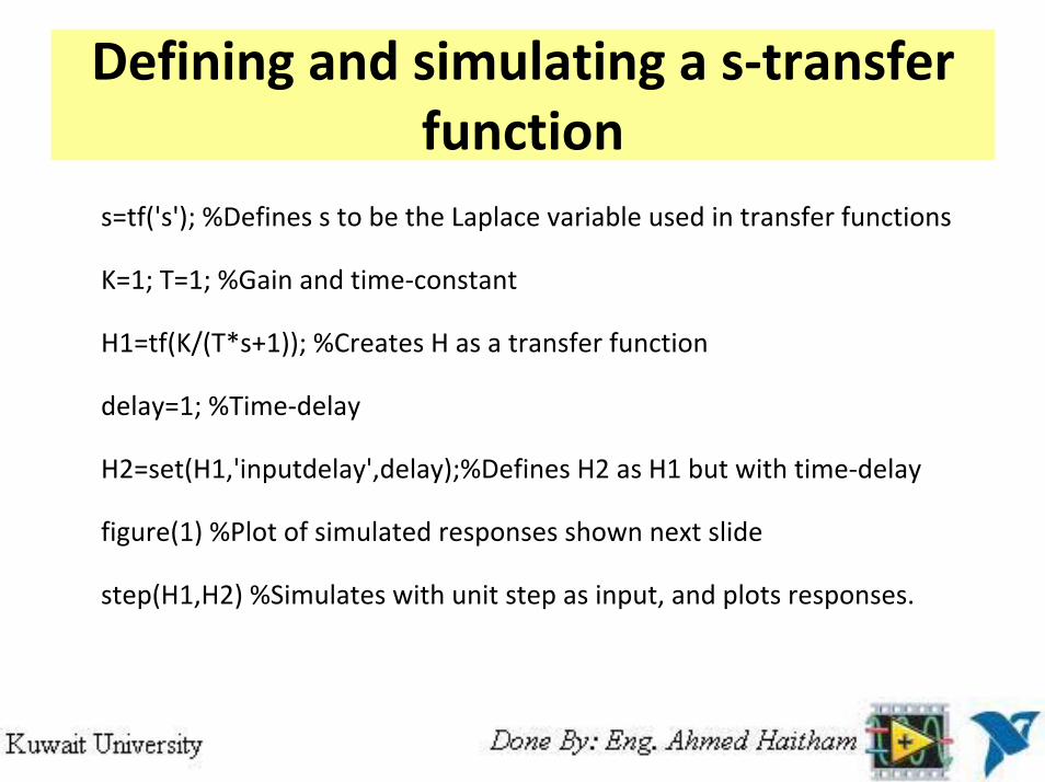
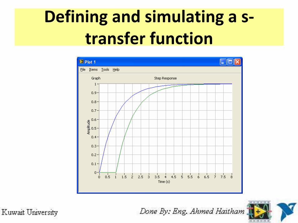
Defining and simulating a s‐transfer function

s=tf('s'); %Defines s to be the Laplace variable used in transfer functions

K=1; T=1; %Gain and time‐constant

H1=tf(K/(T*s+1)); %Creates H as a transfer function

delay=1; %Time‐delay

H2=set(H1,'inputdelay',delay);%Defines H2 as H1 but with time‐delay

figure(1) %Plot of simulated responses shown next slide

step(H1,H2) %Simulates with unit step as input, and plots responses.

Defining and simulating a s‐transfer function

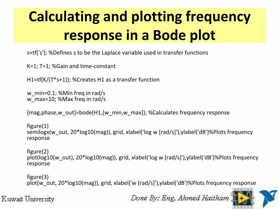
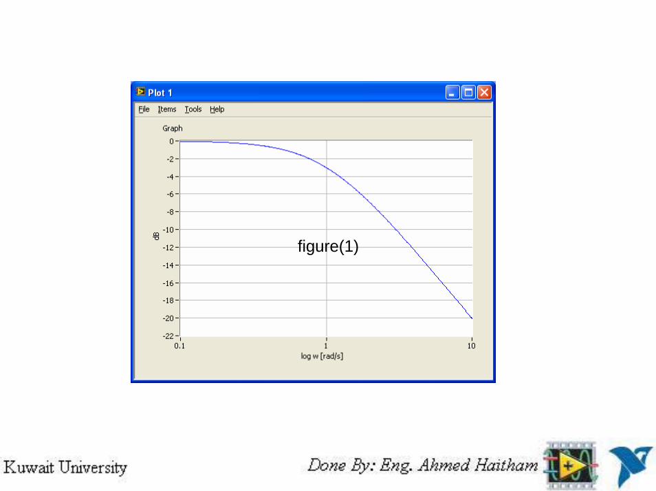
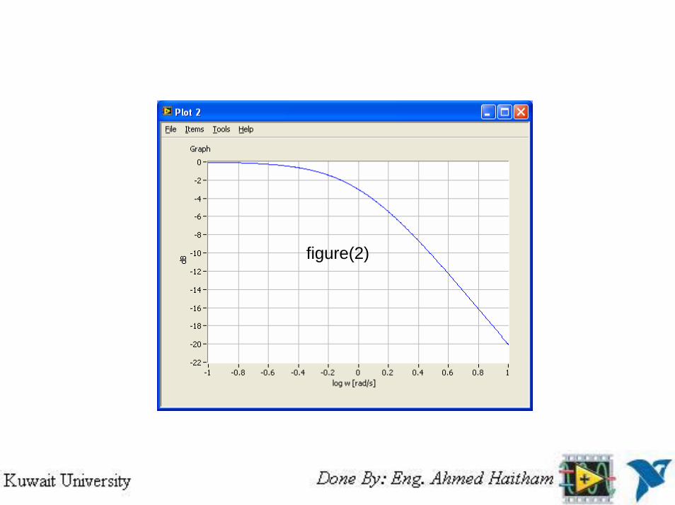
Calculating and plotting frequency response in a Bode plot

s=tf('s'); %Defines s to be the Laplace variable used in transfer functions

K=1; T=1; %Gain and time‐constant

H1=tf(K/(T*s+1)); %Creates H1 as a transfer function

w_min=0.1; %Min freq in rad/sw_max=10; %Max freq in rad/s

[mag,phase,w_out]=bode(H1,[w_min,w_max]); %Calculates frequency response

figure(1)semilogx(w_out, 20*log10(mag)), grid, xlabel('log w [rad/s]'),ylabel('dB')%Plots frequency response

figure(2)plot(log10(w_out), 20*log10(mag)), grid, xlabel('log w [rad/s]'),ylabel('dB')%Plots frequency response

figure(3)plot(w_out, 20*log10(mag)), grid, xlabel('w [rad/s]'),ylabel('dB')%Plots frequency response

figure(1)

figure(2)

figure(3)

Frequency response analysis and simulation of feedback (control) systems

• The next script shows how you can analyze a control system. In this example, the process to be controller is a time‐constant system in series with a time‐delay. The sensor model is just a gain. The controller is a PI controller.

• The time‐delay is approximated with a rational transfer function (on the normal numerator‐denominator form). This is necessary when you want to calculate the tracking transfer function and the sensitivity transfer function automatically using the feedback function. The time‐delay approximation is implemented with the pade function (Padé approximation).

• First, the models are defined using the tf function. The time‐delay is approximated using the pade function. 

Frequency response analysis and simulation of feedback (control) systems

• The control system is simulated using the step function. • The stability margins and corresponding crossover 

frequencies are calculated using the margin function. • The control system transfer functions ‐ namely the loop 

transfer function, tracking transfer funtion and the sensitivity transfer function ‐ are calculated using the series function and the feedback function. 

• These transfer functions are plotted in a Bode diagram using the bode function. 

• Although the system in this example is a continuous‐time system, discrete‐time systems can be analysed in the same way. (With a discrete‐time system, no Padé‐approximation is necessary because time‐delays can be precisely represented in the model.)

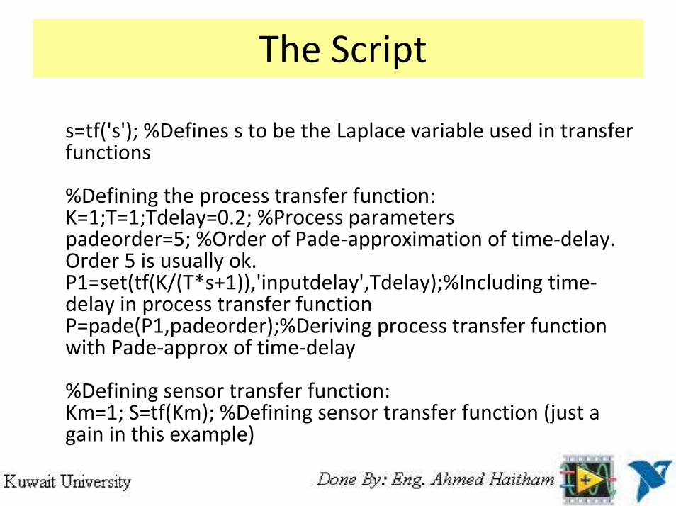
The Script

s=tf('s'); %Defines s to be the Laplace variable used in transfer functions

%Defining the process transfer function:K=1;T=1;Tdelay=0.2; %Process parameterspadeorder=5; %Order of Pade‐approximation of time‐delay. Order 5 is usually ok.P1=set(tf(K/(T*s+1)),'inputdelay',Tdelay);%Including time‐delay in process transfer functionP=pade(P1,padeorder);%Deriving process transfer function with Pade‐approx of time‐delay

%Defining sensor transfer function:Km=1; S=tf(Km); %Defining sensor transfer function (just a gain in this example)

Continue Script

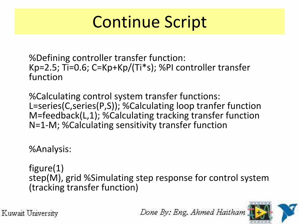
%Defining controller transfer function:Kp=2.5; Ti=0.6; C=Kp+Kp/(Ti*s); %PI controller transfer function

%Calculating control system transfer functions:L=series(C,series(P,S)); %Calculating loop tranfer functionM=feedback(L,1); %Calculating tracking transfer functionN=1‐M; %Calculating sensitivity transfer function

%Analysis:

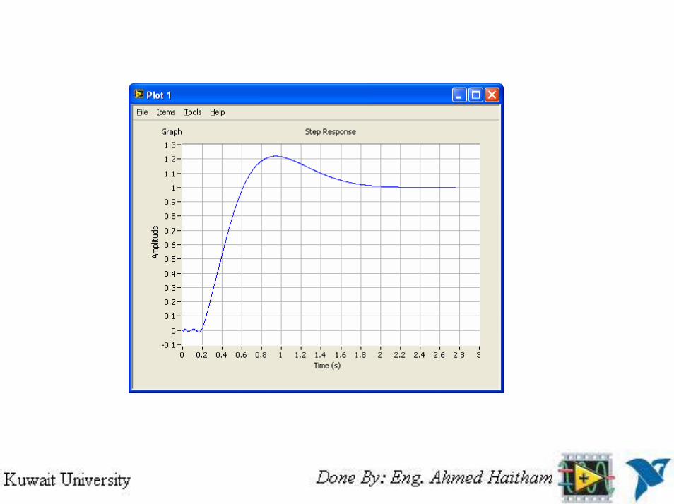
figure(1)step(M), grid %Simulating step response for control system (tracking transfer function)

Continue Script

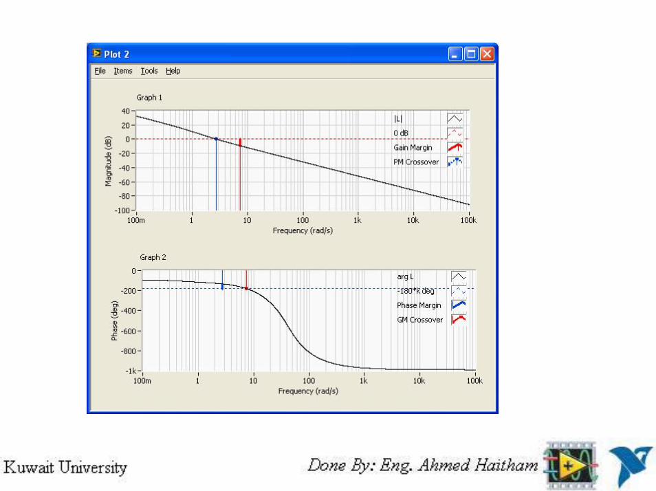
%Calcutating stability margins and crossover frequencies:[gain_margin, phase_margin, gm_freq, pm_freq] = margin(L)%Note: Help margin in LabVIEW shows erroneously parameters in other order than above.

figure(2)margin(L), grid %Plotting L and stability margins and crossover frequencies in Bode diagram

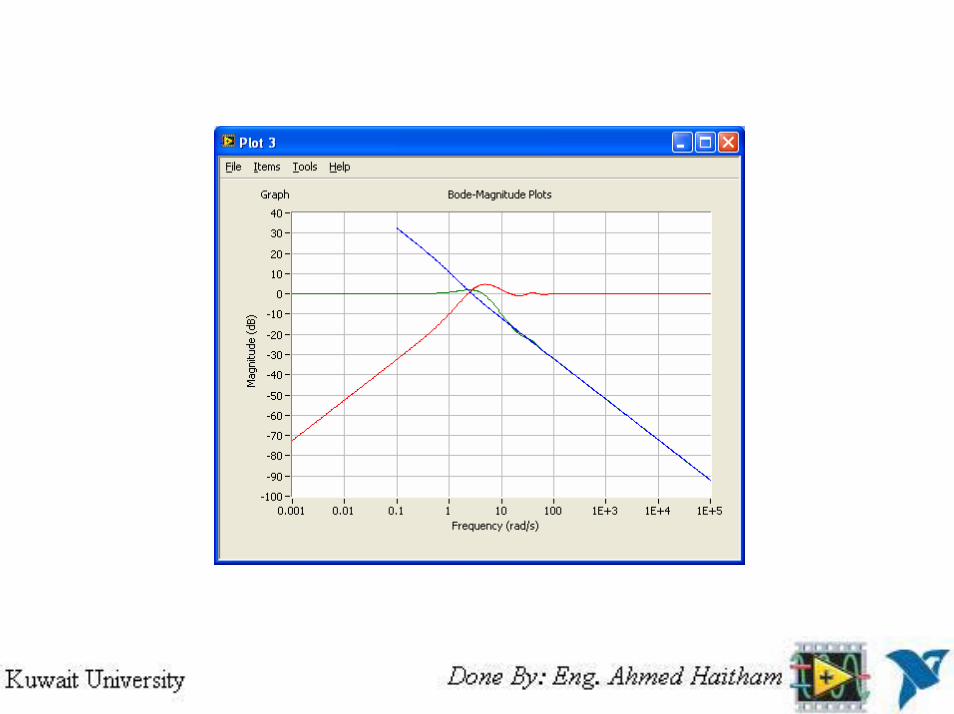
figure(3)bodemag(L,M,N), grid %Plots maginitude of L, M, and N in Bode diagram