Embed Size (px)
Citation preview

Labour Market Programmes and Labour Market
Outcomes: A study of the Swedish Active Labour Market
Interventions
Jerome Adda Monica Costa Dias Costas Meghir
Barbara Sianesi
University College London and Institute for Fiscal Studies
October 2007
Abstract
This paper assesses the impact of Swedish welfare-to-work programmes on labour
market performance including wages, labour market status, unemployment duration and
future welfare-to-work participation. We develop a structural dynamic model of labour
supply which incorporates detailed institutional features of these policies and allows for
selection on observables and unobservables. We estimate the model from a rich admin-
istrative panel data set and show that training programmes - which account for a large
proportion of programmes - have little effect on future outcomes, whereas job experience
programmes have a beneficial effect.
Acknowledgements: This research has benefited from discussions with Eric French,
John Ham and Ken Judd and the comments of two referees. We have also benefited
1

from the opportunity to present this work at the COST workshop (2005), IZA work-
shop on ”Structural Econometric Analysis of Labor Market Policy” (2005), IFAU (2006),
the Tinbergen Institute (2006), the Tilburg University (2006), Technical University of
Lisbon (2006), workshop on ”Labour force participation, labour market dynamics and
programme evaluation” (Venice 2006), Econometric Society European Meeting (2006),
University of Texas-Austin (2006) University of Southern California (2007), Yale Uni-
versity (2007) and North American Winter Meeting of the Econometric Society (2007).
Thanks also to Helge Bennmarker for helpful institutional information and data issues
clarifications. Financial support from IFAU and from the ESRC Centre for the Microe-
conomic Analysis of Fiscal Policy at the IFS is gratefully acknowledged.
2

1 Introduction
Active labour market programmes have become increasingly important in a number of OECD
countries as a way of combating unemployment and helping workers reallocate to new sectors
in the wake of economic shocks. Such programmes have indeed become the centrepiece for
UK employment policy through the ”New Deal” introduced in 1998, and have been a well
established institution in Sweden, where there has been a strong link with benefit eligibility.
In one form or another they have also been an important presence in the US, with programmes
such as the JTPA or other smaller scale training programmes. However, the success of such
programmes is controversial, with a large number of evaluations putting in doubt their overall
effectiveness. Nevertheless, the programmes considered are highly heterogeneous, comprising
anything from job-search assistance, to training and subsidised work.
There is an extensive body of evidence from micro-econometric studies on the effects of var-
ious types of programmes on participants’ subsequent labour market outcomes. Evidence from
different OECD countries shows that subsidised employment has a greater impact than public
training (for which negative effects have at times been estimated). Recent work comparing the
effectiveness of the four options of the New Deal for Young People in the UK similarly finds
that the employment option performs best compared to full-time education and training, the
voluntary sector and the environmental task force (Bonjour et al., 2001; Dorsett, 2006). The
finding that the ’work first’ approach of the employment programme dominates the human
capital approach of the training measure is also in line with the meta-analysis of US welfare-
to-work programmes by Greenberg et al. (2004). Using similar data as in this paper and
based on a non-parametric matching approach, Sianesi (2001a,b) finds that those programmes
providing subsidised workplace experience and on-the-job training at an employer are not only
cheaper, but considerably more effective for participants’ subsequent labour market success
than classroom training courses.
The focus of traditional empirical approaches to evaluation (reviewed extensively in Heck-
3

man et al., 1999) is mostly on statistical robustness; seeking to identify causal effects without
functional-form restrictions, they typically rely on conditional independence assumptions or
the availability of instrumental variables or direct randomisation. Considering mainly reduced-
form models and lacking economic structure, the conventional treatment effect literature is es-
sentially static. However, labour market choices are intrinsically dynamic as current decisions
affect future outcomes and expected future outcomes affect current decisions. To understand
how programmes operate on employment and unemployment durations and on earnings, and
to be in a position to study policy reforms the underlying dynamics have to be modelled.
To achieve this we need to model selection into the (different) programmes and into sub-
sequent employment (cf. Ham and Lalonde, 1996) as economic decisions. Moreover, we need
to account for the incentive structure generated by the institutional framework. For example,
labour market institutions such as the Swedish one (or those of many European countries) add
to the dynamic nature of the problem in two ways: first, by having a large set of different
programmes from which to choose from and second, by linking programme participation to
the renewal of eligibility to unemployment benefits.
To deal with these issues, we develop a dynamic structural model to assess the impact of
a complex welfare-to-work system taking into account how it affects working and future pro-
gramme participation incentives. We model labour supply decisions, programme participation
decisions and earnings, taking into account the institutional features, in particular the eligi-
bility to unemployment insurance and its renewal through programme participation or work.
We allow for selection on unobserved heterogeneity and model explicitly the dynamic selection
choices of forward-looking and optimizing individuals.
We estimate the differential impact of each type of programme or of sequences of pro-
grammes, the short- and long-term effects, and the effects on final and on intermediate out-
comes. We estimate the mean and the full distribution of treatment effects. In the presence of
selection into the programmes based on (unobserved) returns, the average effects uncovered by
4

reduced-form methods may mask important heterogeneity in impacts by types of individuals.
Thus the aim of this paper is to provide a unified framework for evaluating programmes,
recognising their dynamic effects and intertemporal incentives and considering the longer term
impacts on individual careers, including employment and unemployment durations, welfare
dependency and wages. In doing so we specify a model that is capable of simulating the
effects of reforms to the existing system. Thus our approach differs from the recent spate of
evaluations in that we seek to specify and estimate a dynamic economic model of programme
participation, employment and wages. This model is capable both of offering an evaluation of
existing programmes and of simulating the effects of alternative policies.
The Swedish labour market programmes have been considered before1, though never in such
a systematic way as we propose here. Furthermore, we have put together a detailed data set
which follows a cohort of unemployed for a number of years. The employment status data has
been linked to earnings records allowing us to follow career outcomes of workers for a number
of years, free from recall bias.
We find that training programmes seem to have no beneficial impact on the treated. On the
contrary, they postpone exit from unemployment due to the lock-in effect, whereby treated are
deterred from moving into employment while on the programme, which can be used to renew
unemployment insurance eligibility. Subsidised employment seems to be more beneficial, par-
ticularly to high ability individuals. First, it speeds up transitions into employment although
not enough to recover from the lock-in effect. Second, it seems to have some impact on wages
although less than usual job experience. And third, treated individuals of high ability enjoy
longer employment spells after treatment.
The next section discusses the Swedish institutional context, the essence of which we try to
capture in our dynamic structural model, and describes the data used in our analysis. Section 3
sets up the model. Section 4 presents the estimated effects of treatment and section 5 discusses
1e.g. Forslund and Krueger (1997) and Sianesi (2001a,b and 2004).
5

the predicted outcomes of alternative policy scenarios. Finally section 6 concludes the paper.
2 Data and institutional background
2.1 The Swedish labour market policy
Sweden runs one of the world’s most generous welfare policies targeted at the unemployed. We
briefly describe the prevalent and most relevant features of Swedish labour market institutions
of the late nineties (1996-1998, corresponding to the time period covered by the data) that will
set the ground for our model.
Unemployment insurance (UI) in Sweden amounts to 80% of the individuals salary in the
previous job up to a ceiling of about SEK16,500 per month. To first become eligible to 14
months of UI benefits, an individual needs to have worked for a minimum of 80 days over 5
calendar months during the previous 12 months.2 After meeting such requirement, eligibility
to UI can always be renewed through an additional 80 days over 5 calendar months of work or
treatment through one or more of the many programmes offered to the unemployed.
There are a great number of alternative treatments being offered at any time to unemployed
individuals, in particular job subsidies, trainee replacement schemes, vocational labour market
training (AMU), relief work, and work practice schemes (including work experience replace-
ment, ALU, and workplace introduction, API). In this paper we distinguish between subsidised
employment, which includes the first two treatments mentioned above, and all the other pro-
grammes in assessing their differential impact on labour market performance. In what follows,
the latter will be called training programmes.3
2There is also a membership condition, requiring payment of the (almost negligible) membership fees to the
UI fund for at least 12 months prior to the claim. However, opting out of membership seems to be a rare event
and we deal with UI membership as if it was compulsory.3Although alternative aggregate rules could have been used and argued for, our choice was to classify the
programmes according to their compensation regime as this reflects their relative closeness to the labour market.
6

There have been numerous policy changes although the 1996-1998 period has been remark-
ably stable. Notwithstanding, reforms occurred in July 1997, regarding the eligibility rules
to unemployment compensation, and in September 1997, regarding the compensation level.
These have been minor changes and we disregard them in the model. Perhaps the major pol-
icy change after our observational time window occurred in February 2001 when the possibility
to renew eligibility to UI through programme participation was abolished. Using our model
and results, we will assess the potential impacts of such policy change.4
2.2 Data
This section briefly discusses the main data related issues. More details can be found in
Appendix C.
Data sources The data set we use is drawn from four different administrative data sets
which have been merged for the purpose of the study:
• The Unemployment Register Handel provides information from August 1991 onwards on
unemployment spells, programme participation spells and the subsequent labour market
status of those who are deregistered (e.g. employment, education, inactivity or ‘lost’
(attrition)).
• The Akstat data base provides information on unemployment compensation from January
1994 onwards.
• The Kontrolluppgifts-registry provides employment information by employer from Jan-
uary 1990 onwards. This is employer provided data for tax purposes and is reported
A finer classification could have disclosed more detailed information about the programmes and will be the
subject of further work.4In future work we plan to explore the use of the most relevant policy changes to validate a structural
model.
7

yearly. It includes the period of employment and the total earnings (which we also des-
ignate by wages) over the period by employer. Reported earnings are equally split over
working period on a monthly basis. These are total earnings, not adjusted for hours
worked.
• The Sysreg dataset provides information on educational achievement (highest educational
level) by calendar year, starting in 1990.
The different data sets are merged together using the individual’s unique social security
number. The data cover the whole working age population in Sweden.
Sample selection From the data we select the group individuals becoming unemployed
during 1996 and follow them up to December 1998. For simplicity, we focus on a relatively
homogeneous group. Selection was ruled by two main criteria: (i) the relative importance
of the group in terms of size and expected returns from treatment and (ii) the nature of
the decision process among the individuals of the group. Our final sample is composed of
individuals with the following characteristics:
• Males - by excluding females we avoid having to deal with fertility decisions.
• Unskilled - these are disproportionately represented among the unemployed. We choose
individuals having completed no more than 1 to 2 years of high school and not upgrading
during the observation period (this is true for 95% of the unskilled population of the age
group being considered - see below).
• Aged 26 to 30 at the time of their sample inflow - young individuals have been the
object of attention of both policies and empirical research for two reasons: (i) they are to
become the major labour force group in the near future and (ii) their perceived plasticity
facilitates learning and adaptation to new conditions or environments. We focused on a
young group outside the educational years to avoid dealing with the educational decisions.
8

• Not disabled or self-employed - these individuals face different conditions and policies.
Using these selection criteria, our data set contains 14,370 individuals who all start an
unemployment spell in 1996. From these data we have excluded individuals for whom the
information from the unemployment register and from the employer is incompatible. These
are individuals who have a relatively long history of past employment as derived from the
employer-provided data, but who are not eligible for unemployment benefits as detailed in the
unemployment registry data. About 20% of the sample has been excluded on these grounds.5
We have also dropped individuals eligible to unemployment insurance at sample inflow but with
no previous employment history. These amount to less then 2% of the sample. Estimation
used a randomly selected 20% sub-sample of these cleaned and selected data.
Labour market activity In each calendar month from inflow to December 1998, the in-
dividual’s activity is classified in one of the four alternatives: employment, unemployment,
subsidised employment or training programme. When more than one activity is present in
any given month, we selected the one that lasted longest in that month. Since the employer-
provided data is not as reliable as the unemployment register, we gave preference to unem-
ployment information in case of conflict. This means that employment is the residual activity
whenever a positive wage is simultaneously observed.
We do not distinguish between part- and full-time employment. While on part-time em-
ployment, individuals may still be entitled to UI (a share of the full amount) and have priority
access to treatment as compared to unregistered individuals. However, part-time employment
contributes towards renewing UI eligibility, just as full time employment does. We therefore
decided to classify both types of jobs in the “employment” state.
5Although membership to UI funds is voluntary and is a pre-requisite to eligibility, it is unlikely that it
explains this disparity between eligibility and employment history as the number of workers that opt out from
UI funds seems to be small.
9

Programme occurrences were only considered if in long spells, defined as lasting for more
than 2 months. In such case, treatment spells are split in 4 months periods and considered
as sequences of treatment events. While such simplification reduces the dimensionality of our
problem, it also corresponds to the patterns found in the data. Descriptive analysis has shown
that the duration of the treatment spells peaks at 3 to 4 months.6
However rich and effective the data is in following individuals over their working life, it
sometimes happens that we lose contact with one individual in a given month during our
observational time window, meaning that the agent is neither registered as unemployed, in
a treatment spell or in paid work. This may happen because, for example, the individual
moves into education, out of the country or into inactivity (unregistered unemployment). We
censor the history of affected individuals from that moment onwards. This affects 30% of the
individuals in the sample.
Variables Based on the historical information back to 1990, we constructed a number of
variables to characterise the individuals’ state: (i) working experience, which is simply the
cumulated number of months in employment since January 1990; (ii) remaining eligibility
to UI in months, which varies from 0 to 14, is used up while in unemployment and can be
recovered through employment or programme participation; and (iii) the criterion to renew
full eligibility to UI (14 months), which measures the time in work or treatment since the last
unemployment spell.
6It should be noticed that although the policy requirement to renew UI eligibility is 5 months in either
employment or treatment, we will use a 4-month rule in the model discussed below. Such choice reflects the
different criteria used by the employment services and in our study in measuring time in each labour market
status. Calendar months are used in both cases. As explained before, the employment services require the
agent to work for 80 days over 5 months, meaning that in some of these months the agent may work for as
little as 1 day. Our criterion, however, is to use the predominant labour market status over the calendar month
and to require 4 months of employment/treatment. By being more demanding, our measure will under-predict
the accumulated experience towards renewing eligibility.
10
2.3 Descriptive statistics
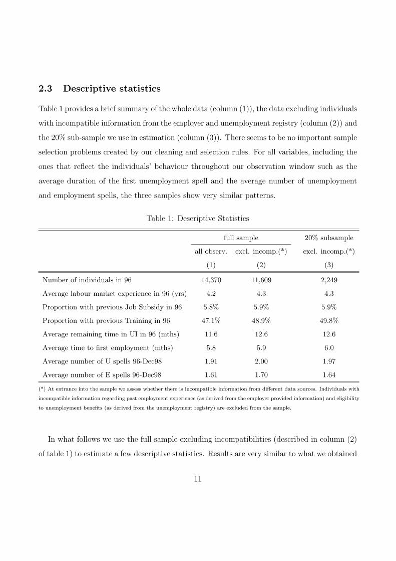
Table 1 provides a brief summary of the whole data (column (1)), the data excluding individuals
with incompatible information from the employer and unemployment registry (column (2)) and
the 20% sub-sample we use in estimation (column (3)). There seems to be no important sample
selection problems created by our cleaning and selection rules. For all variables, including the
ones that reflect the individuals’ behaviour throughout our observation window such as the
average duration of the first unemployment spell and the average number of unemployment
and employment spells, the three samples show very similar patterns.
Table 1: Descriptive Statistics
full sample 20% subsample
all observ. excl. incomp.(*) excl. incomp.(*)
(1) (2) (3)
Number of individuals in 96 14,370 11,609 2,249
Average labour market experience in 96 (yrs) 4.2 4.3 4.3
Proportion with previous Job Subsidy in 96 5.8% 5.9% 5.9%
Proportion with previous Training in 96 47.1% 48.9% 49.8%
Average remaining time in UI in 96 (mths) 11.6 12.6 12.6
Average time to first employment (mths) 5.8 5.9 6.0
Average number of U spells 96-Dec98 1.91 2.00 1.97
Average number of E spells 96-Dec98 1.61 1.70 1.64
(*) At entrance into the sample we assess whether there is incompatible information from different data sources. Individuals with
incompatible information regarding past employment experience (as derived from the employer provided information) and eligibility
to unemployment benefits (as derived from the unemployment registry) are excluded from the sample.
In what follows we use the full sample excluding incompatibilities (described in column (2)
of table 1) to estimate a few descriptive statistics. Results are very similar to what we obtained
11
using the 20% subsample but are more precise.
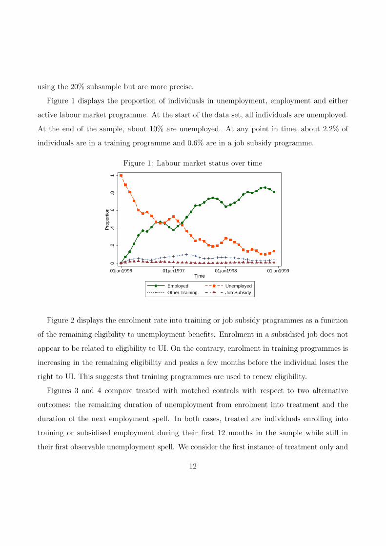
Figure 1 displays the proportion of individuals in unemployment, employment and either
active labour market programme. At the start of the data set, all individuals are unemployed.
At the end of the sample, about 10% are unemployed. At any point in time, about 2.2% of
individuals are in a training programme and 0.6% are in a job subsidy programme.
Figure 1: Labour market status over time
0.2
.4.6
.81
Pro
port
ion
01jan1996 01jan1997 01jan1998 01jan1999Time
Employed UnemployedOther Training Job Subsidy
Figure 2 displays the enrolment rate into training or job subsidy programmes as a function
of the remaining eligibility to unemployment benefits. Enrolment in a subsidised job does not
appear to be related to eligibility to UI. On the contrary, enrolment in training programmes is
increasing in the remaining eligibility and peaks a few months before the individual loses the
right to UI. This suggests that training programmes are used to renew eligibility.
Figures 3 and 4 compare treated with matched controls with respect to two alternative
outcomes: the remaining duration of unemployment from enrolment into treatment and the
duration of the next employment spell. In both cases, treated are individuals enrolling into
training or subsidised employment during their first 12 months in the sample while still in
their first observable unemployment spell. We consider the first instance of treatment only and
12
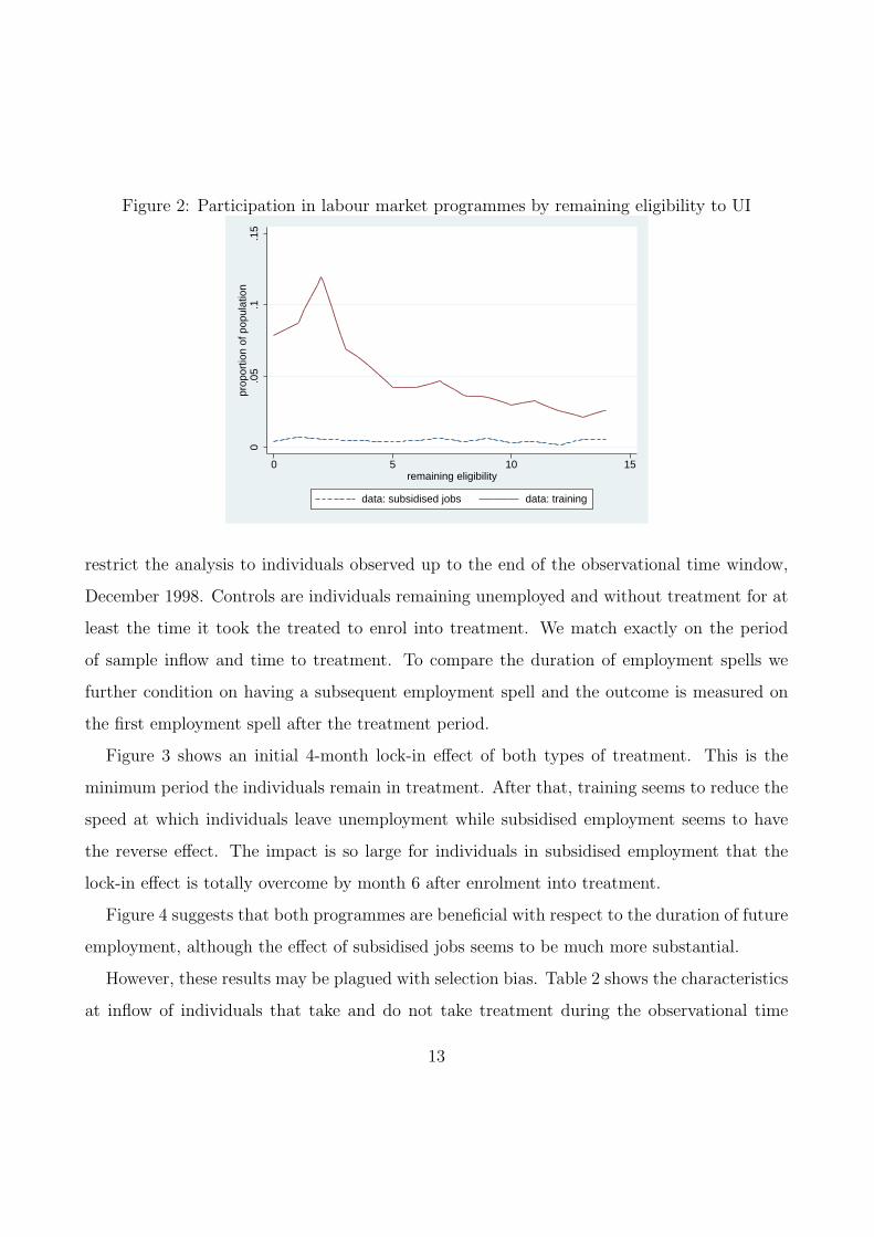
Figure 2: Participation in labour market programmes by remaining eligibility to UI
0.0
5.1
.15
prop
ortio
n of
pop
ulat
ion
0 5 10 15remaining eligibility
data: subsidised jobs data: training
restrict the analysis to individuals observed up to the end of the observational time window,
December 1998. Controls are individuals remaining unemployed and without treatment for at
least the time it took the treated to enrol into treatment. We match exactly on the period
of sample inflow and time to treatment. To compare the duration of employment spells we
further condition on having a subsequent employment spell and the outcome is measured on
the first employment spell after the treatment period.
Figure 3 shows an initial 4-month lock-in effect of both types of treatment. This is the
minimum period the individuals remain in treatment. After that, training seems to reduce the
speed at which individuals leave unemployment while subsidised employment seems to have
the reverse effect. The impact is so large for individuals in subsidised employment that the
lock-in effect is totally overcome by month 6 after enrolment into treatment.
Figure 4 suggests that both programmes are beneficial with respect to the duration of future
employment, although the effect of subsidised jobs seems to be much more substantial.
However, these results may be plagued with selection bias. Table 2 shows the characteristics
at inflow of individuals that take and do not take treatment during the observational time
13
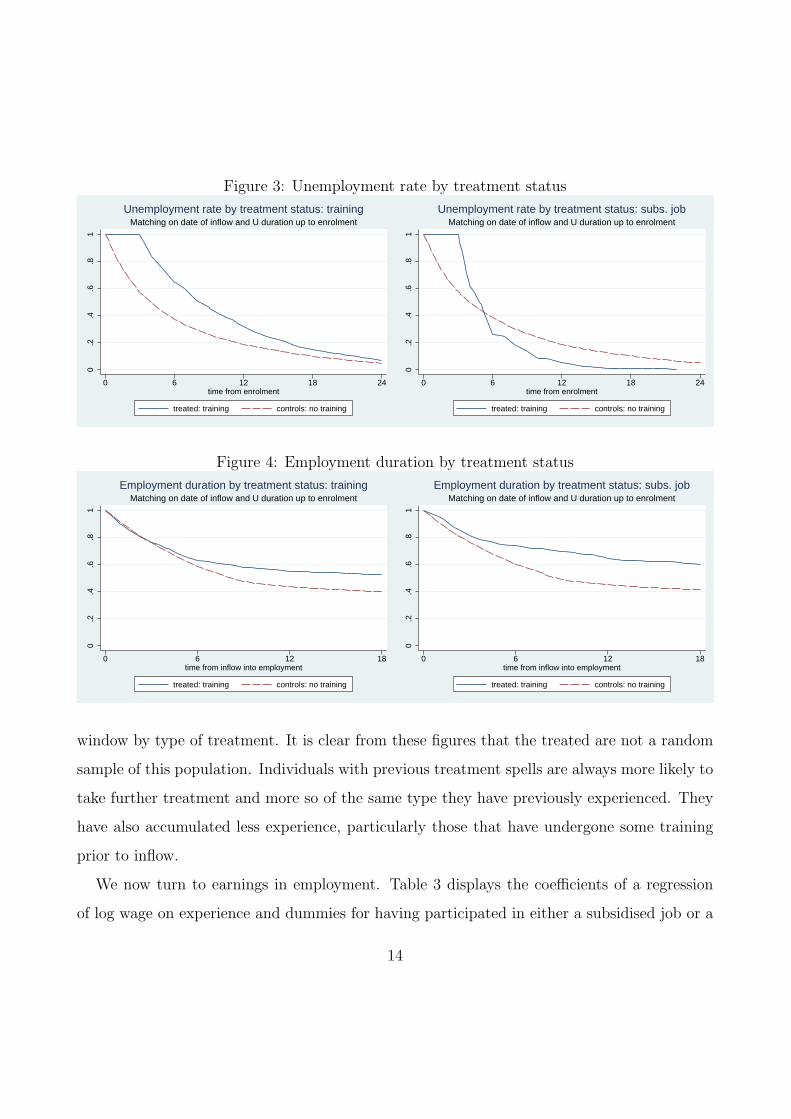
Figure 3: Unemployment rate by treatment status
0.2
.4.6
.81
0 6 12 18 24time from enrolment
treated: training controls: no training
Matching on date of inflow and U duration up to enrolmentUnemployment rate by treatment status: training
0.2
.4.6
.81
0 6 12 18 24time from enrolment
treated: training controls: no training
Matching on date of inflow and U duration up to enrolmentUnemployment rate by treatment status: subs. job
Figure 4: Employment duration by treatment status
0.2
.4.6
.81
0 6 12 18time from inflow into employment
treated: training controls: no training
Matching on date of inflow and U duration up to enrolmentEmployment duration by treatment status: training
0.2
.4.6
.81
0 6 12 18time from inflow into employment
treated: training controls: no training
Matching on date of inflow and U duration up to enrolmentEmployment duration by treatment status: subs. job
window by type of treatment. It is clear from these figures that the treated are not a random
sample of this population. Individuals with previous treatment spells are always more likely to
take further treatment and more so of the same type they have previously experienced. They
have also accumulated less experience, particularly those that have undergone some training
prior to inflow.
We now turn to earnings in employment. Table 3 displays the coefficients of a regression
of log wage on experience and dummies for having participated in either a subsidised job or a
14

Table 2: Treated versus non-treated within observational time window - characteristics at
inflow
Subsidized job Training
non-treated treated non-treated treated
past experience in months 51.1 49.6 52.4 47.3
% had subsidised jobs in the past 5.7% 10.3% 5.4% 7.3%
% participated in training in the past 48.6% 57.4% 45.0% 60.5%
Notes: Table shows characteristics at inflow of individuals that take and do not take treatment during the observa-
tional time window (January 96 to December 98), by type of treatment.
training programme during the observational window. The analysis is conditional on having
had no treatment prior to inflow. We compute the treatment effects using both OLS and a
fixed effects regression. Cross section estimates (columns (1) and (2) in the table) suggest that
subsidised jobs have a positive impact on earnings of almost 3.5%. On the contrary, training
seems to have a detrimental effect on earnings of over 9%. However, these numbers are unlikely
to be consistent estimates of the treatment effects if selection into treatment is not random.
The next two columns in table 3 display the first differences estimates of a similar regression.
By using first differences, we remove fixed differences in productivity at individual level. While
individuals experiencing unemployment see a 2% decrease in their wage, the effects of both
labour market programmes are positive, 7.5% for subsidised jobs and 5.9% for training. There
are at least three possible explanations for these results. The first, of course, is that treatment
genuinely improves the earnings of participants. The second is that some mechanism like the
Ashenfelter’s dip rules participation: agents that have suffered a drop in earnings before be-
coming unemployed are more likely to enrol into treatment. However, a simple comparison
of the earnings growth rates of treated and non-treated before an unemployment spell does
not support this hypothesis. The third explanation is that programme participation affects
15

Table 3: Determinants of log earnings
OLS First differences
Coefficient sd. err. Coefficient sd. err.
(1) (2) (3) (4)
experience (log) 0.155 0.011 -0.610 0.353
Job subsidy 0.035 0.014 0.075 0.044
Training -0.093 0.007 0.059 0.021
unemployment 0.011 0.007 -0.023 0.005
constant 8.963 0.045 0.0089 0.005
observations 98,843 93,748
Notes: Regressions are conditional on no programme participation prior to first ob-
servation. The observations in these regressions are the months in employment of all
individuals included in the selected sample with no incompatibilities. This is why
there are many more observations used in these regressions than individuals in the
sample. The regression in first differences discards the first working observation for
each individual with at least one employment spell over the observational window.
selection into employment and the selection process generates these results. Programme par-
ticipation provides treatment and renews eligibility to UI. As a consequence, unemployment
may become a more valued option after treatment, increasing the reservation wage and making
individuals more selective about which jobs to accept.
The large differences between estimates obtained using OLS and fixed effects show how
important it is to take into account unobserved heterogeneity related to labour productivity.
In the next section we develop a model that explicitly addresses the dynamic selection issues
and allows for unobserved heterogeneity.
16

3 The model
3.1 An overview
We model labour supply and programme participation for a group of workers who have become
unemployed early on in their career. The model incorporates the main institutional features
of the Swedish active labour market programmes faced by this cohort in the late nineties.
Individuals are assumed to be forward looking and to make fully informed decisions about
their working lives. The framework we use has its origins in the seminal work by Eckstein and
Wolpin (1989a and b).
The model is set in discrete time with one period corresponding to a month. Because the
individuals are young when they enter the sample we solve their optimisation problem as if
they were infinitely lived. In each time period, the individual chooses an activity to maximise
the expected present value of rewards (utility) subject to constraints (e.g. ”is an offer of
a job available?”) and to available information. Possible (mutually exclusive) activities are
employment, unemployment and participation in one of two programmes - subsidised job and
training.
Thus, while out of work, the individual may be offered a job or a place on a programme.
The individual then assesses the relative costs and benefits of participation, including those
expected in the future, and chooses the best option. Individuals receive offers at different rates,
depending on their characteristics. These may change over time, as a result of the individual’s
actions.
Once in a job, the individual receives a wage determined by her/his characteristics and
subject to random shocks. Individuals who receive sufficiently bad stochastic shocks may move
into unemployment. We do not separate between voluntary and involuntary job separations
because the data does not seem to support such distinction. According to previous estimates
of our model, where a job destruction probability was introduced instead of allowing for some
17
permanent taste from employment, the job destruction probability is zero and the model is
incapable of reproducing the transitions into employment, both from unemployment and the
programmes. Accordingly, we also do not account for differences between quits and layoffs in
terms of eligibility to UI while in reality the former would not be eligible. This is also in line
with the fact that UI sanctions are rare in Sweden. We therefore abstract from this aspect of
the unemployment policy.
There are several sources of dynamics in the model: (i) participation in programmes affects
future benefits while out of work, future earnings and the chances of receiving job and treatment
offers; and (ii) employment affects experience, earnings and the benefits while out of work.
3.2 A formal description of the model
3.2.1 The state space
In each period the individual decides about labour market status. We consider four possible
alternatives, employment (E), unemployment (U), subsidised employment (J) and training
(T ). The decision at each point in time is determined by the information set at the individual’s
disposal. We assume the relevant information is described by a set of relevant variables, some
observable and others unobservable by the econometrician.
The observable state space includes work experience (e); the remaining number of months of
entitlement to UI benefits (u where u is below a cap u = 14 months); the accumulated number
of periods working or in a programme since UI eligibility was last exhausted (m where m is
below a cap m = 4);7 the number of spells in subsidised employment and training programmes
(pJ and pT , respectively), and the number of such spells completed at the start of the current
out-of-work spell if applicable (sJ and sT , respectively); the exogenous variables (x) including
7Although the true policy parameter is m = 5 we choose to use m = 4. See the data section for a justification
of this choice.
18

region of residence.8 The set of possible values of these observable variables constitute the
state space Ω; at each point in time, t agent i draws a point in this state space, Ωit.
The state space for the unobservable variables is denoted by Γ where Γit is the point drawn
by individual i at time t. Γ includes a number of variables: (i) a productivity innovation,
ν, which arrives with probability π if the agent is employed or in a subsidised job and is
also realised by non-employed individuals receiving a job offer; (ii) job and programme offers,
which arrive with probabilities ol for l = E, J, T ; and (iii) the transitory taste shocks, εl for
l = E, J, T .
Finally, we also allow for two sources of unobserved heterogeneity: θW , which explains per-
manent differences in productivity (wage) levels; and θE, which explains permanent differences
in job attachment. In what follows we call the former ability and the latter taste for employ-
ment. We denote by θ the 2-factor unobserved heterogeneity, θ =(θW , θE
). Both sources
of heterogeneity have a discrete distribution. Following some experimentation the former has
three points of support and the latter two.
3.3 The individual’s problem
Let dit describe the labour market status of individual i at time t with possible values l =
U,E, J, T . This is the decision variable. dit = l means that alternative l has been selected in
period t.
The problem of individual i in period τ is to select the optimal sequence of feasible activities
over the future, ditt=τ,..., conditional on the contemporaneous information set, (Ωiτ , Γiτ , θi),
maxditt=τ,...
Eτ
∞∑t=τ
∑
l∈U,E,J,Tβt−τ1(dit = l)Rl
it (Ωit, Γit, θi)
∣∣∣∣∣∣Ωiτ , Γiτ , θi
where β is the discount rate, Rl represents the per period reward or utility function when
8sJ and sT determine the amount of compensation while in unemployment, not pJ and pT .
19

labour market option l is selected and Eτ is the expectations operator conditional on the
available information at time τ .
This maximisation problem is subject to a number of restrictions, including the laws of
motion for the state variables and the feasibility of the different labour market options in
each period. We now describe the per-period reward functions and the restrictions to the
maximisation problem.
3.4 Per period reward functions
Contemporaneous utility is assumed to be logarithmic in income. Income is modelled as
a dynamic process. Working and programme participation affect future earnings while in
employment, as well as income while out of work given its link to the market wage.
The contemporaneous utility from employment The market wage for an individual of
ability type θW with e periods of working experience and (pJ , pT ) treatments is w(eit, pJit, p
Tit, θ
Wi ).
The actual earnings are also determined by the transitory productivity shock, ν, so that
wit = w(eit, pJit, p
Tit, θ
Wi ) exp(νit).
Following the patterns in the data, we model the persistence in ν through a positive prob-
ability but smaller than 1 probability of receiving a wage innovation in each period (π).9 So,
for an individual who has two sequential employment periods,
wit+1 =
wit with probability π
w(eit+1, pJit+1, p
Tit+1, θ
Wi ) exp(νit+1) with probability 1− π
If a wage innovation is received while in employment, it is drawn from the distributionN (0, σ1).
While out of work, a new job offer is drawn from the distribution of wage innovations, N (0, σ0).
9We have experimented with an AR(1) process for the innovation ν. However such model could not reproduce
important patterns in the data such as the transitions from employment.
20
The current reward of employment for individual i at time t can now be expressed as,
RE (Ωit, Γit, θi) = ln(w
(eit, p
Jit, p
Tit, θ
Wi
)exp (νit)
)+ θE
i + εEit
where the taste for employment is captured by the unobserved heterogeneity term, θE. The
transitory taste shock, εE, is uncorrelated over time and has distribution N (0, σ2E).
The contemporaneous utility from unemployment The period utility from unemploy-
ment depends on the eligibility status to UI. An eligible individual (u > 0) is entitled to a
proportion α of the market wage for a worker of similar characteristics up to a ceiling, B.10 An
ineligible individual (u = 0) is entitled to a flat social security rate, b. The contemporaneous
utility function for an unemployed individual i at time t is
RU (Ωit, Γit, θ) =
ln(UIit) = ln(min
αw
(eit, s
Jit, s
Tit, θ
Wi
), B
)if uit > 0
ln(b) if uit = 0
where sJ and sT measure the number of programmes the individual has participated in up
to the beginning of the current out-of-work spell and UIit is the amount of unemployment
insurance the individual receives while entitled.
The contemporaneous utility from subsidised employment We define a subsidised
employment spell to equal the number of months required for the renewal of benefit eligibility
(m). An individual may have consecutive spells in subsidised emplyment. This treatment does
not change the individual’s work experience. Instead, the productivity effects are measured by
an indicator of the number of past treatment spells, pJit. The two other differences to regular
employment are that subsidised employment does not accrue utility θEi and the taste shock is
specific to the programme. The reward function for the whole m-months period on a subsidised
10This is a simplification of the actual policy, which states that the individual is entitled to a proportion α
of the earnings in the last employment up to a ceiling, B.
21
job is,
RJ (Ωit, Γit, θ) =1− βm
1− βln
(w(eit, p
Jit, p
Tit, θi) exp (νit)
)+ εJ
it
where t is the first treatment period. The transitory taste shock, εJ , is assumed to be uncor-
related over time and has distribution N (0, σ2J).
In consecutive subsidised employment spells, the productivity innovation is allowed to ex-
hibit some persistence in a fashion similar to what is described above for consecutive employ-
ment periods.
The contemporaneous utility from training Finally, the contemporaneous returns to
training programmes depend on whether the minimum working experience requirement for
UI has been fulfilled in the past. Again, we only consider long spells, lasting for at least m
months, and the longer spells are split into subsequent spells of exactly m months. The per-
period income is either the UI benefit or the social security flat rate subsidy, depending on
whether e is larger or smaller than m. The reward function for the whole m periods is,
RT (Ωit, Γit, θ) =
1−βm
1−βln(UIit) + εT
it if eit ≥ m
1−βm
1−βln(b) + εT
it if eit < m
where the transitory taste component, εTit, is uncorrelated over time and has distribution
N (0, σ2T ).
3.5 Transitions
The feasible set of activities in any period is restricted by the present activity and the arrival
of offers for the alternative activities l = E, J, T . We follow the patterns observed in data,
excluding direct transitions from employment into the programmes and from subsidised jobs
into training. Conditional on receiving an offer, the individual will then decide whether to
accept it or to remain (or become) unemployed. We assume the time intervals to be sufficiently
22

small to ensure that at most one offer arrives in each period. The offer arrival probabilities,
ol for l = E, J, T , are allowed to vary with the individual’s characteristics. They are modelled
as a logistic function of the activity in the previous period, past programme participation and
region of residence. Treatment offers also depend on remaining eligibility time, to reflect the
fact that the case officers in the job-centres will often prioritise finding a placement for those
who are running out of benefits.11
3.6 The intertemporal value functions
Conditional on receiving an offer, the individual’s decision is based on the comparison of the
present and future value of each option. This process is described by the comparison of value
functions for each alternative activity. We now describe these value functions. We denote
by V lit the inter-temporal value of option l at time t for individual i. It is a function of all
contemporaneous observable and unobservable variables but we omit this dependence for ease
of notation.
The value of employment depends on its contemporaneous returns, RE (Ωit, Γit, θi), and
on future prospects as affected by current employment while assuming optimal decisions in
the future. Employed individuals can always remain employed for as long as the value of
employment remains high enough. The outside option is to move into unemployment. The
value of being employed can then be written as,
V Eit = RE (Ωit, Γit, θi) +
β(1− π)EεE
[max
V U
it+1, VEit+1
∣∣ θi,Ωit, wit+1 = wit, dit = E]+
βπE(εE ,ν)
[max
V U
it+1, VEit+1
∣∣ θi, Ωit, wit+1 6= wit, dit = E]
where the two last terms represent the continuation values under the two alternatives depend-
ing on the realisation or not of a wage innovation. An innovation occurs with probability π
11In offering treatment, priority is given to individuals close to exhausting their eligibility to UI.
23

(3rd line in the equation). The operators EεE and EεE ,ν stand for the expectations with respect
to εE or (εE, ν) at time t+1, respectively. In all that follows, Eα represents the expected value
with respect to the random variable α at t+1. The expectations are conditional on the present
(time t) information and use the laws of motion described below to learn about the state space
at t + 1 which is the (omitted) argument of V lt+1 for l = U,E. The notation we use below is in
line with the one just discussed.
The value of unemployment While unemployed, the individual may receive an offer of
any type (employment and the two programme types). The decision of whether or not to
move will depend on the relative value of the two alternatives, where unemployment is always
a possibility. Thus, the value of unemployment at period t is
V Uit = RU (Ωit, Γit, θi) +
βoE (Ωit+1, dit = U) E(εE ,ν)
[max
V U
it+1, VEit+1
∣∣ θi, Ωit, dit = U]+
βoJ (Ωit+1, dit = U) E(εJ ,ν)
[max
V U
it+1, VJit+1
∣∣ θi, Ωit, dit = U]+
βoT (Ωit+1, dit = U) EεT
[max
V U
it+1, VTit+1
∣∣ θi, Ωit, dit = U]+
β[1− oE (Ωit+1, dit = U)− oJ (Ωit+1, dit = U)− oT (Ωit+1, dit = U)
]E
[V U
it+1
∣∣iθi, Ωit, dit = U
]
where the terms in lines 2, 3 and 4 correspond to the possibility of receiving a job, subsidised
employment or training offers, respectively. The last term deals with the possibility that no
offer to start at t + 1 arrives, in which case the individuals has no option but to remain
unemployed.
The value of subsidised employment and training The current utility while on a sub-
sidised job, RJ (Ωit, Γit, θi), accounts for the duration of the spell (m months). In m months
time the individual will be weighing up the options and if possible will be deciding whether to
move into employment or a new subsidised employment spell.12 The value of a subsidised job
12Direct transitions into training programmes from subsidised jobs have been excluded as they are not
observed in the data.
24

is
V Jit = RJ (Ωit,Γit, θi) +
βmoE (Ωit+m, dit = J) E(εE ,ν)
[max
V U
it+m, V Eit+m
∣∣ θi, Ωit, dit = J]+
βmoJ (Ωit+m, dit = J) (1− π)EεJ
[max
V U
it+m, V Jit+m
∣∣ θi, Ωit, wit+m = wit, dit = J]+
βmoJ (Ωit+m, dit = J) πE(εJ ,ν)
[max
V U
it+m, V Jit+m
∣∣ θi,Ωit, wit+m 6= wit, dit = J]+
βm[1− oE (Ωit+m, dit = J)− oJ (Ωit+m, dit = J)
]E
[V U
it+m
∣∣ θi, Ωit, dit = J]
The value of the training option is similarly given by
V Tit = RT (Ωit, Γit, θi) +
βmoE (Ωit+m, dit = T ) E(εE ,ν)
[max
V U
it+m, V Eit+m
∣∣ θi, Ωit, dit = T]+
βmoJ (Ωit+m, dit = T )E(εJ ,ν)
[max
V U
it+m, V Jit+m
∣∣ θi, Ωit, dit = T]+
βmoT (Ωit+m, dit = T ) EεT
[max
V U
it+m, V Tit+m
∣∣ θi, Ωit, dit = T]+
βm[1− oE (Ωit+m, dit = T )− oJ (Ωit+m, dit = T )− oT (Ωit+m, dit = T )
]E
[V U
it+m
∣∣ θi, Ωit, dit = T]
3.7 Dynamics of the information set
The rules governing the dynamics of the observable state variables depend on the present
activity. Conditional on activity, they follow simple, deterministic rules.
Working experience is accumulated on the job only, each month in employment representing
an additional period.
Eligibility to UI is determined by the variable u, which measures the remaining months of
UI entitlement. u is limited by a maximum number of entitlement periods, u, and is “used
up” while the individual is unemployed: for each period in unemployment, the individual loses
entitlement to one period of UI benefits. The associated variable m defines the eligibility
25

requirement. To first gain eligibility to the full u months of insured unemployment the indi-
vidual must complete m months in regular employment. After that, full eligibility is regained
by either completing a further m periods on a job or by participating in programmes for the
same length of time. Since we are only considering long programme spells, lasting at least for
m months, programme enrolment will always lead to full eligibility after the initial working
requirement is fulfilled. Both m and u are zero at the start of working life. At the start of our
observational time window, however, they will generally be different from zero as individuals
have had time to accumulate some working and treatment experience.
Programme experience is accumulated through programme participation. We consider pro-
gramme spells lasting for exactly m and split longer spells in sequences of treatments. We only
consider the impact of the first treatment spell of each type.
3.8 Estimation method
The full structural model is estimated by maximum likelihood using a nested optimisation
algorithm where the inner routine solves the structural problem of the worker conditional on
the model parameters and the outer routine maximises the likelihood function (see Rust, 1994,
for a description of these sort of algorithms). To ensure stationarity, experience is assumed to
have no impact on earnings after 20 years of work.
Unobserved heterogeneity is assumed to follow a discrete distribution. We allowed for 6
different unobserved types, resulting from a combination of 3 ability types and 2 preference
types. Unobserved heterogeneity affects decisions through a number of dimensions, including
earnings, returns to experience and returns to treatment, employment and treatment offer
probabilities and job attachment. We estimate the distribution of unobserved herogeneity
using non-parametric maximum likelihood following (see Heckman and Singer, 1984).
The sample selection process, which chooses 25-30 years old males flowing into unemploy-
ment during 1996, creates an initial conditions problem: working experience and accumulated
26

programme participation at entrance are endogenous in the sense that they are correlated with
unobserved heterogeneity. While we do not deal with it here, we plan to do so in the future.
The full likelihood function can be found in appendix B.
As described in the data section above, estimation was based on a random sub-sample of
20% of the individuals in the administrative data that start an unemployment spell during
1996.
4 Estimation results
4.1 Estimated parameters
The model is fully described by a total of 40 parameters and all the estimates are presented in
appendix A. Here we provide a brief description of some of the more meaningful parameters.
Table 4: Unobserved heterogeneity: joint distribution of the two factors
Heterogeneity in preferences
Low taste for E High taste for E
Ability
low 5.14% 3.02%
medium 17.80% 58.25%
high 15.72% 0.06%
Table 4 shows the distribution of unobserved heterogeneity over the population. Over 75%
of our sample is concentrated in the “medium-ability” group, with most of them having “high
taste from employment”. In contrast, we find few people in the tails with “lower” or “higher”
ability. One interpretation is that unobservable characteristics are not playing a very important
role in explaining observed behaviour.
27
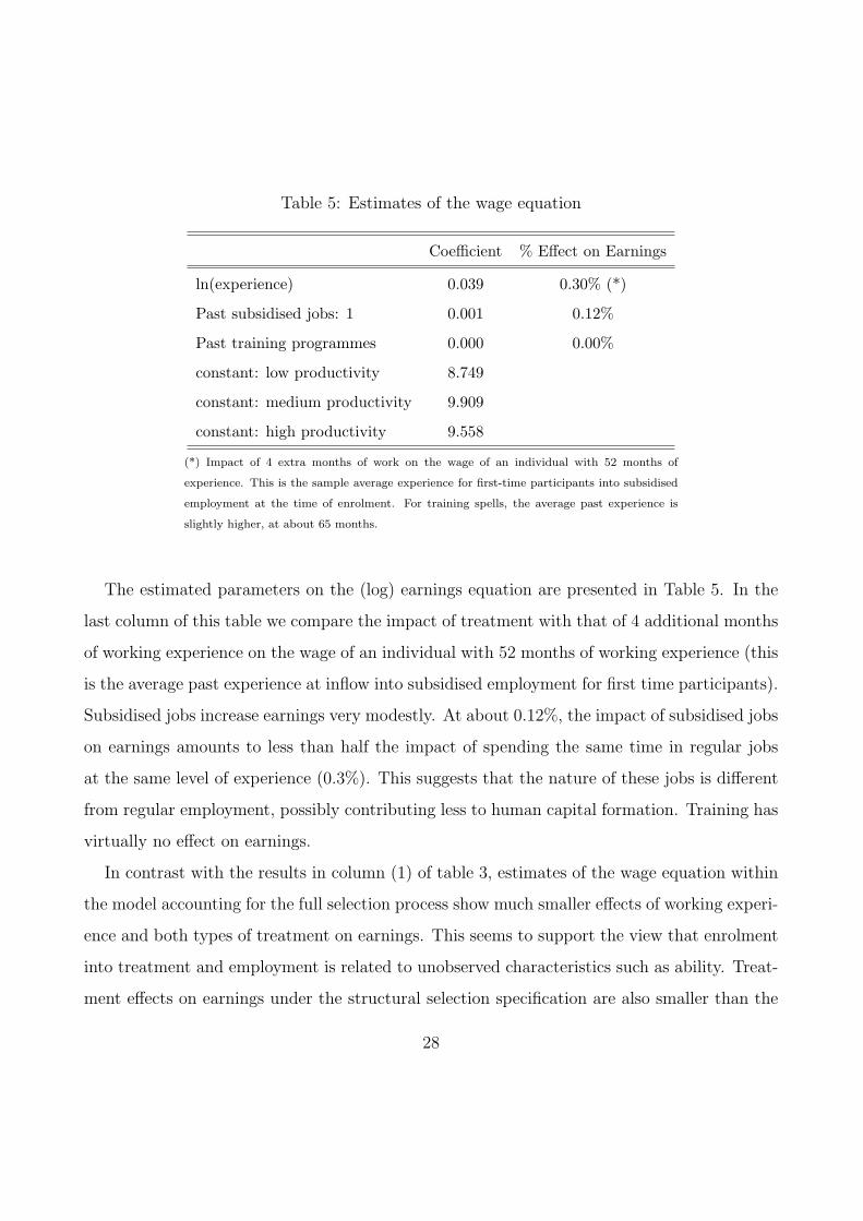
Table 5: Estimates of the wage equation
Coefficient % Effect on Earnings
ln(experience) 0.039 0.30% (*)
Past subsidised jobs: 1 0.001 0.12%
Past training programmes 0.000 0.00%
constant: low productivity 8.749
constant: medium productivity 9.909
constant: high productivity 9.558
(*) Impact of 4 extra months of work on the wage of an individual with 52 months of
experience. This is the sample average experience for first-time participants into subsidised
employment at the time of enrolment. For training spells, the average past experience is
slightly higher, at about 65 months.
The estimated parameters on the (log) earnings equation are presented in Table 5. In the
last column of this table we compare the impact of treatment with that of 4 additional months
of working experience on the wage of an individual with 52 months of working experience (this
is the average past experience at inflow into subsidised employment for first time participants).
Subsidised jobs increase earnings very modestly. At about 0.12%, the impact of subsidised jobs
on earnings amounts to less than half the impact of spending the same time in regular jobs
at the same level of experience (0.3%). This suggests that the nature of these jobs is different
from regular employment, possibly contributing less to human capital formation. Training has
virtually no effect on earnings.
In contrast with the results in column (1) of table 3, estimates of the wage equation within
the model accounting for the full selection process show much smaller effects of working experi-
ence and both types of treatment on earnings. This seems to support the view that enrolment
into treatment and employment is related to unobserved characteristics such as ability. Treat-
ment effects on earnings under the structural selection specification are also smaller than the
28
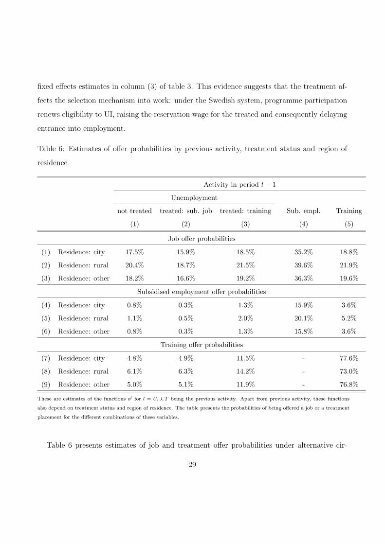
fixed effects estimates in column (3) of table 3. This evidence suggests that the treatment af-
fects the selection mechanism into work: under the Swedish system, programme participation
renews eligibility to UI, raising the reservation wage for the treated and consequently delaying
entrance into employment.
Table 6: Estimates of offer probabilities by previous activity, treatment status and region of
residence
Activity in period t− 1
Unemployment
not treated treated: sub. job treated: training Sub. empl. Training
(1) (2) (3) (4) (5)
Job offer probabilities
(1) Residence: city 17.5% 15.9% 18.5% 35.2% 18.8%
(2) Residence: rural 20.4% 18.7% 21.5% 39.6% 21.9%
(3) Residence: other 18.2% 16.6% 19.2% 36.3% 19.6%
Subsidised employment offer probabilities
(4) Residence: city 0.8% 0.3% 1.3% 15.9% 3.6%
(5) Residence: rural 1.1% 0.5% 2.0% 20.1% 5.2%
(6) Residence: other 0.8% 0.3% 1.3% 15.8% 3.6%
Training offer probabilities
(7) Residence: city 4.8% 4.9% 11.5% - 77.6%
(8) Residence: rural 6.1% 6.3% 14.2% - 73.0%
(9) Residence: other 5.0% 5.1% 11.9% - 76.8%
These are estimates of the functions ol for l = U, J, T being the previous activity. Apart from previous activity, these functions
also depend on treatment status and region of residence. The table presents the probabilities of being offered a job or a treatment
placement for the different combinations of these variables.
Table 6 presents estimates of job and treatment offer probabilities under alternative cir-
29
cumstances depending on previous activity, whether or not the individual has been treated in
the past and region of residence. Activity in period t − 1 strongly affects offer probabilities.
Being in a subsidised job spell more than doubles the probability of being offered a job in the
next period (column (4) as compared with the remaining columns, rows(1)-(3)). This probably
reflects a transformation of the subsidised job into regular employment where the individual
remains in the same firm, possibly doing a similar task but now in the regular workforce. How-
ever, having had subidised jobs in the past does not seem to help job search. On the contrary,
it has a small negative impact on job offer probabilities, suggesting it might give a bad signal
to potential employers (column (2) versus columns (1) and (3), rows (1)-(3)). Training does
not seem to affect offer probabilities other than those of training: past training spells make
training offers more likely to arrive (column (3), rows (7)-(9)) while having been in training
at t − 1 makes it very probable to be able to continue (column (5), rows (7)-(9)). These es-
timates together with the also high offer probabilities of subisdised employment for agents in
subsidised employment are partly determined by the continuation of the same treatment spell
over 4 months.
4.2 Fit of the model
In this section we show some evidence on the fit of the model along with a discussion of the
directly observable patterns of the data. In assessing the fit we use the distribution of initial
conditions in our sample and simulate the individual decisions throughout the observable
period. Each individual is simulated 30 times. We then compare the patterns created by the
simulated data with what is observed in the real data.
Table 7 displays the data and simulated month-to-month transition probabilities between
alternative labour market states. Rows (5) and (10) show the proportion of observations falling
in each state and, as expected, the simulations reproduce observable data very closely. This
is confirmed in figure 5, which presents the proportion of individuals in each state over time
30

Table 7: Fit of Model - transitions between labour market states
U E S T
Real Data:
(1) unemployment (U) 0.781 0.177 0.005 0.038
(2) employment (E) 0.064 0.936 0.000 0.000
(3) subsidised job (S) 0.133 0.084 0.783 0.000
(4) training (T) 0.142 0.039 0.003 0.826
(5) total 0.320 0.610 0.007 0.063
Simulated Data:
(6) unemployment (U) 0.785 0.174 0.005 0.036
(7) employment (E) 0.066 0.934 0.000 0.000
(8) subsidised job (S) 0.133 0.080 0.787 0.000
(9) training (T) 0.139 0.041 0.003 0.817
(10) total 0.325 0.607 0.008 0.060
from the moment of sample inflow. The dashed and full lines stand for simulated and real
data, respectively. The simulated data seem to reproduce the average evolution of labour
market status quite closely but fails to capture the seasonal patterns (the current version of
the estimates does not allow for seasonal variation but this will be incorporated in future
versions of the model).
Another particularly important feature is the pattern of transitions between different states.
The remaining rows in table 7 present the data (rows (1) to (4)) and model (rows (6) to (9))
transition probabilities. Again, the simulated pattern is very closed to the observed one.
Figures 6 and 7 compare data and model regarding the probabilities of inflow into treatment
and employment by remaining months of eligibility to unemployment benefit. While we are able
to reproduce the inflows into treatment quite closely, the model does very badly in accounting
31

Figure 5: Fit of the model - labour market status over time
0.2
.4.6
.81
prop
ortio
n of
pop
ulat
ion
0 10 20 30 40(calendar) time
data: unemployment simulation: unemploymentdata: employment simulation: employmentdata: subsidised jobs simulation: subsidised jobsdata: training simulation: training
Figure 6: Fit of the model - Transitions into treatment by remaining eligibility time
0.0
5.1
.15
prop
ortio
n of
pop
ulat
ion
0 5 10 15remaining eligibility
data: subsidised jobs simulation: subsidised jobsdata: training simulation: training
for the inflows into employment. Instead of the generally upward sloping curve displayed by
the data, which suggests compositional changes in the pool of unemployment by eligibility
time, the model captures a slightly downward curve due to the increasing costs of remaining
32
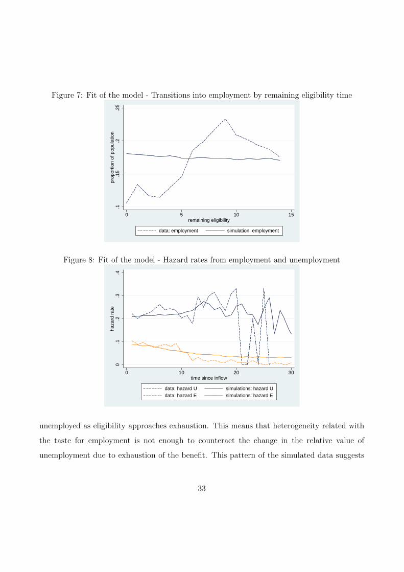
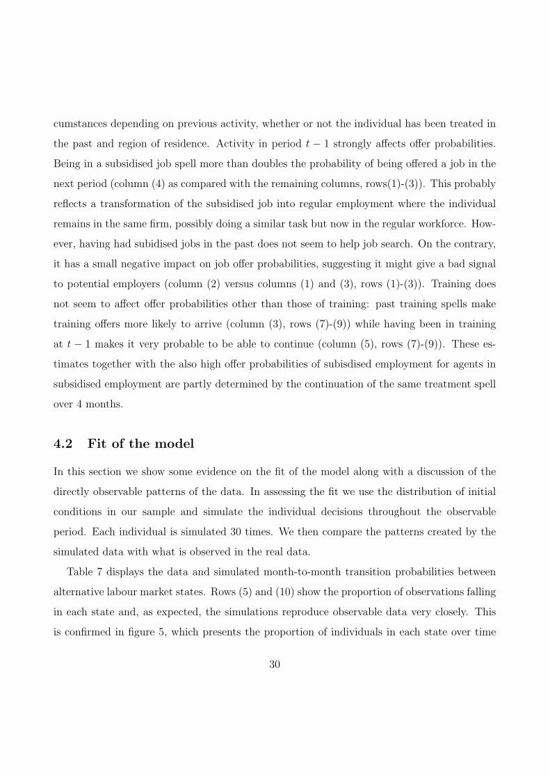
Figure 7: Fit of the model - Transitions into employment by remaining eligibility time
.1.1
5.2
.25
prop
ortio
n of
pop
ulat
ion
0 5 10 15remaining eligibility
data: employment simulation: employment
Figure 8: Fit of the model - Hazard rates from employment and unemployment
0.1
.2.3
.4ha
zard
rat
e
0 10 20 30time since inflow
data: hazard U simulations: hazard Udata: hazard E simulations: hazard E
unemployed as eligibility approaches exhaustion. This means that heterogeneity related with
the taste for employment is not enough to counteract the change in the relative value of
unemployment due to exhaustion of the benefit. This pattern of the simulated data suggests
33

that an additional source of heterogeneity might be needed and requires careful attention in
future work.
Instead, heterogeneity related to the taste for employment is much more effective in captur-
ing duration dependence on the job. Figure 8 shows that the evolution of the hazard rates from
both employment and unemployment is captured quite well by the model. Figure 8 also shows
a peak in the outflows from unemployment around a duration of 14 months, which is captured
by the model as a response to benefit exhaustion. According to figures 6 and 7, such peak
arises from the transitions into training near or at benefit exhaustion, not from transitions into
employment.
Table 8: Fit of the Model - Distribution of the logarithm of observed earnings
Data Model
Mean 9.68 9.69
St. deviation 0.42 0.52
Percentile:
1 8.00 8.35
5 8.92 8.81
25 9.57 9.36
50 9.72 9.71
75 9.89 10.04
95 10.24 10.53
99 10.62 10.89
Tables 8 and 9 show how close the model reproduces the data on earnings. Table 8 shows
that the distribution of earnings among workers is very close in the two datasets. Table 9
then assesses the correlation between earnings among the employed and different individual
34
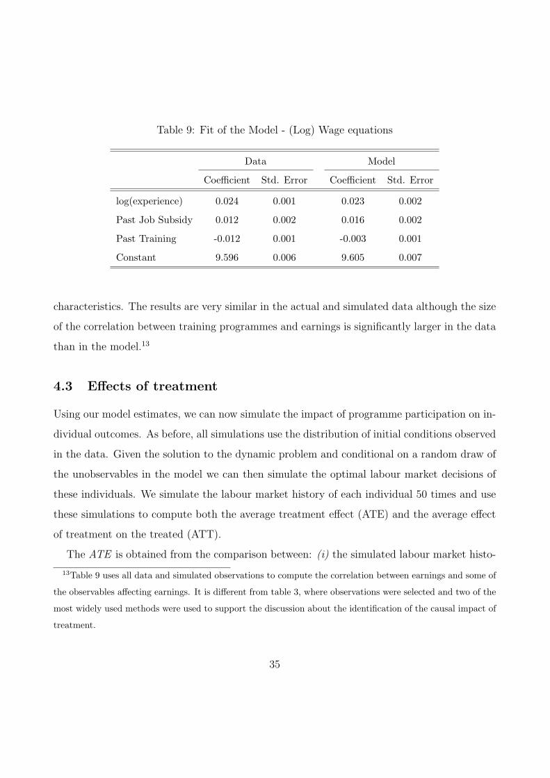
Table 9: Fit of the Model - (Log) Wage equations
Data Model
Coefficient Std. Error Coefficient Std. Error
log(experience) 0.024 0.001 0.023 0.002
Past Job Subsidy 0.012 0.002 0.016 0.002
Past Training -0.012 0.001 -0.003 0.001
Constant 9.596 0.006 9.605 0.007
characteristics. The results are very similar in the actual and simulated data although the size
of the correlation between training programmes and earnings is significantly larger in the data
than in the model.13
4.3 Effects of treatment
Using our model estimates, we can now simulate the impact of programme participation on in-
dividual outcomes. As before, all simulations use the distribution of initial conditions observed
in the data. Given the solution to the dynamic problem and conditional on a random draw of
the unobservables in the model we can then simulate the optimal labour market decisions of
these individuals. We simulate the labour market history of each individual 50 times and use
these simulations to compute both the average treatment effect (ATE) and the average effect
of treatment on the treated (ATT).
The ATE is obtained from the comparison between: (i) the simulated labour market histo-
13Table 9 uses all data and simulated observations to compute the correlation between earnings and some of
the observables affecting earnings. It is different from table 3, where observations were selected and two of the
most widely used methods were used to support the discussion about the identification of the causal impact of
treatment.
35

ries of individuals flowing into unemployment during 1996 and (ii) their simulated histories had
they been forced into treatment at inflow into unemployment in 1996. We do this separately
for both subsidised employment and training.
The ATT is obtained from the comparison between: (i) the simulated labour market histo-
ries of individuals flowing into unemployment during 1996 and joining a programme at some
point during the first 2 simulated years and (ii) the simulated labour market history of the
same subgroup of individuals had they been refused participation on that first treatment they
intended to take. That is, the ATT measures the impact on individuals that are observed in
the simulations to select into treatment.14
For both the ATE and the ATT, we then simulate individual choices over the next 3 years in
both treatment scenarios (being and not being treated) and compute the effects by comparing
treated and controls. The effects arise as a combination of impacts of treatment on productivity
levels, job offer probabilities and a change in the returns to unemployment due to the way
treatment affects eligibility to unemployment benefits.
There are two substantial differences between the ATE and the ATT. First, of course, is
the nature of the parameter: ATE is the average impact on a randomly selected individual
while ATT is the impact on individuals that self-select into treatment. And second, different
definitions of treatment are used in each case: the ATE measures the impact of treatment at
inflow into unemployment while ATT measures the impact of treatment at a moment in the
first unemployment spell selected by the individual.
The first two columns of Table 10 display the ATE on income and activity over the 3 years
that follow completion of treatment. Both programmes have a negative effect on earnings.
This is especially true for training, which reduces earnings by 1.1%. Training also substantially
decreases time in employment (by about 5%). Two factors explain this effect: training induces
14This treated group is similar to the one used to plot the impact of treatment on the duration of unemploy-
ment and subsequent employment spells as displayed in figures 3 and 4.
36
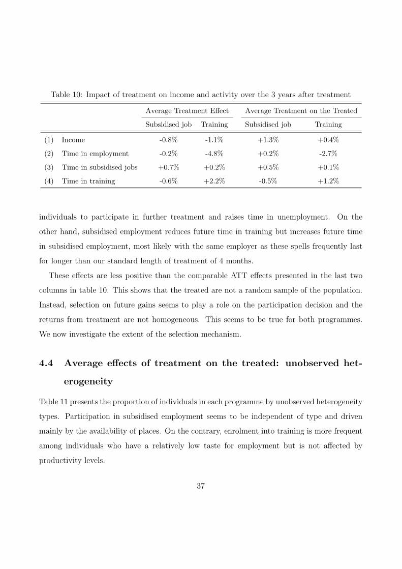
Table 10: Impact of treatment on income and activity over the 3 years after treatment
Average Treatment Effect Average Treatment on the Treated
Subsidised job Training Subsidised job Training
(1) Income -0.8% -1.1% +1.3% +0.4%
(2) Time in employment -0.2% -4.8% +0.2% -2.7%
(3) Time in subsidised jobs +0.7% +0.2% +0.5% +0.1%
(4) Time in training -0.6% +2.2% -0.5% +1.2%
individuals to participate in further treatment and raises time in unemployment. On the
other hand, subsidised employment reduces future time in training but increases future time
in subsidised employment, most likely with the same employer as these spells frequently last
for longer than our standard length of treatment of 4 months.
These effects are less positive than the comparable ATT effects presented in the last two
columns in table 10. This shows that the treated are not a random sample of the population.
Instead, selection on future gains seems to play a role on the participation decision and the
returns from treatment are not homogeneous. This seems to be true for both programmes.
We now investigate the extent of the selection mechanism.
4.4 Average effects of treatment on the treated: unobserved het-
erogeneity
Table 11 presents the proportion of individuals in each programme by unobserved heterogeneity
types. Participation in subsidised employment seems to be independent of type and driven
mainly by the availability of places. On the contrary, enrolment into training is more frequent
among individuals who have a relatively low taste for employment but is not affected by
productivity levels.
37

Table 11: Selection into treatment by unobserved heterogeneity - proportion of treated in
group
Low taste for E High taste for E
Ability Ability
All low medium high low medium high
% in Subsidised job 2.2% 2.0% 1.9% 2.2% 2.6% 2.2% 0.0%
% in Training 15.7% 21.8% 22.5% 22.3% 10.7% 11.6% 10.5%
Table 12 displays the ATT by types of unobserved heterogeneity. All types of individuals
benefit from treatment in terms of income but these effects arise through different channels
depending on the individual’s characteristics and type of treatment.
Subsidised employment leads individuals with a lower taste for employment to reduce future
employment participation and gains arise essentially from the prolonged eligibility to unem-
ployment insurance and improved chances of further subsidised employment spells. Individuals
with a higher taste for employment increase future time in regular and subsidised employment
by over 1% of their time during the following three years (or about 11 days), independently
of productivity level, and this is the main source of additional income. In both cases, future
take up of training is reduced as this is mostly a substitute for subsidised employment in the
attempt to prolong eligibility to unemployment benefits.
By contrast, training has a smaller but still positive impact on future income, of about
0.4% (row (2)). If we break up this impact by remaining eligibility time, the impact is larger,
at about 1.6%, for individuals within six months of benefit exhaustion but is negative, about
-0.5%, for individuals farther away from exhaustion.15 Individuals with a higher taste for
employment are less likely to participate in training programmes and they also benefit less in
15These results are not in the table and can be obtained from the authors under request.
38
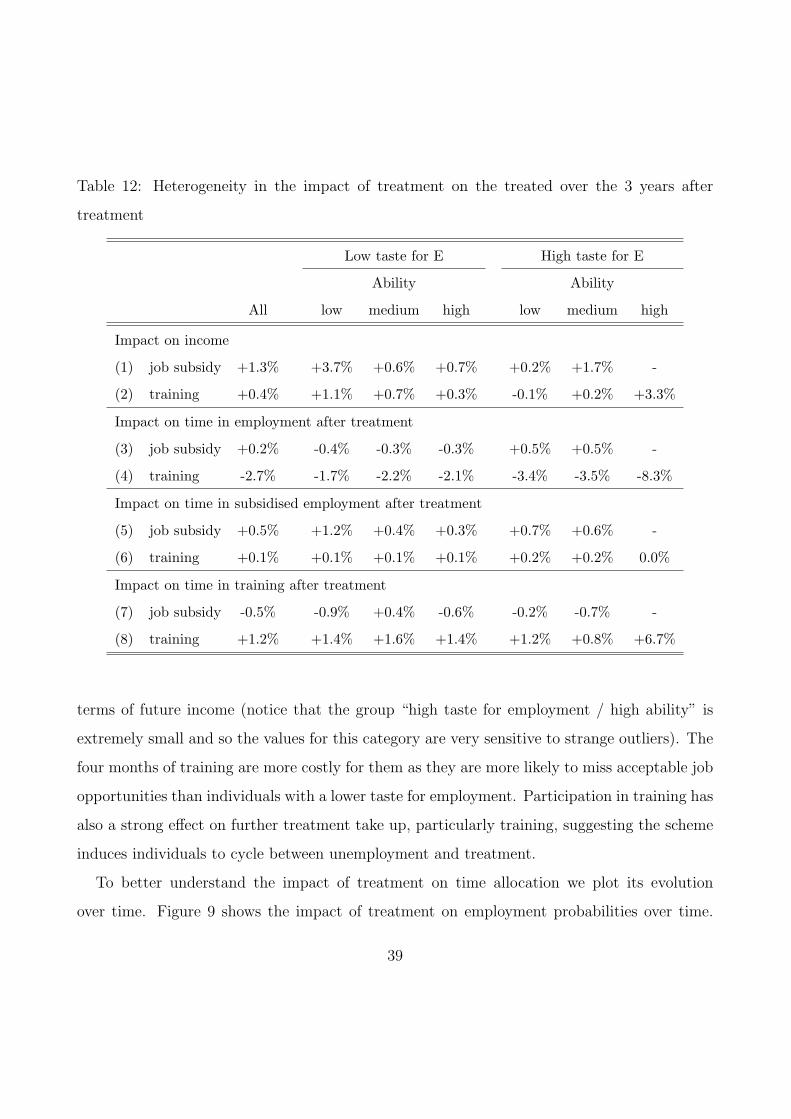
Table 12: Heterogeneity in the impact of treatment on the treated over the 3 years after
treatment
Low taste for E High taste for E
Ability Ability
All low medium high low medium high
Impact on income
(1) job subsidy +1.3% +3.7% +0.6% +0.7% +0.2% +1.7% -
(2) training +0.4% +1.1% +0.7% +0.3% -0.1% +0.2% +3.3%
Impact on time in employment after treatment
(3) job subsidy +0.2% -0.4% -0.3% -0.3% +0.5% +0.5% -
(4) training -2.7% -1.7% -2.2% -2.1% -3.4% -3.5% -8.3%
Impact on time in subsidised employment after treatment
(5) job subsidy +0.5% +1.2% +0.4% +0.3% +0.7% +0.6% -
(6) training +0.1% +0.1% +0.1% +0.1% +0.2% +0.2% 0.0%
Impact on time in training after treatment
(7) job subsidy -0.5% -0.9% +0.4% -0.6% -0.2% -0.7% -
(8) training +1.2% +1.4% +1.6% +1.4% +1.2% +0.8% +6.7%
terms of future income (notice that the group “high taste for employment / high ability” is
extremely small and so the values for this category are very sensitive to strange outliers). The
four months of training are more costly for them as they are more likely to miss acceptable job
opportunities than individuals with a lower taste for employment. Participation in training has
also a strong effect on further treatment take up, particularly training, suggesting the scheme
induces individuals to cycle between unemployment and treatment.
To better understand the impact of treatment on time allocation we plot its evolution
over time. Figure 9 shows the impact of treatment on employment probabilities over time.
39

Figure 9: Re-employment probabilities over time after treatment
−.4
−.3
−.2
−.1
0ef
fect
on
empl
oym
ent r
ate
0 6 12 18 24 30 36time from enrolment into treatment in months
subsidised job training
ATT: Effect of treatment on employment probabilities
There are very strong negative effects of both types of treatment immediately after enrolment,
the lock-in effect. But as treatment finishes, individuals in subsidised employment flow into
regular employment very fast and become slightly more likely to be employed after 1 year from
enrolment than if they had not been treated. The recovery from the lock-in effect is much
slower for individuals in training and they are always less likely to be employed in the future
than if they had not participated in the training programme. As training raises the value of
unemployment but does not change the value of employment, it will lead individuals to remain
out of work for longer.
Figures 10 to 12 show how the duration of unemployment and employment spells are af-
fected by treatment. Figure 10 plots the remaining duration of the first unemployment spell
after enrolment into treatment. The graph displays the behaviour of treated and comparable
controls. It shows that both types of treatment have a positive impact on the duration of
unemployment. In the case of subsidised jobs, the increased speed at which treated move into
jobs is not enough to compensate for the lock-in effect of treatment. Training, however, if
anything has a zero effect on the speed at which unemployed find jobs, thus further prolonging
40

Figure 10: Duration of unemployment from time of enrolment into treatment by type of
treatment: comparison between treated and controls0
.2.4
.6.8
1P
ropo
rtio
n in
une
mpl
oym
ent
0 6 12 18 24time from start of spell in months
treated: subsidised job controls: subsidised jobtreated: training controls: training
Duration of unemployment
Figure 11: Duration of first employment spell after treatment by type of treatment: comparison
between treated and controls
0.2
.4.6
.81
Pro
port
ion
in e
mpl
oym
ent
0 6 12 18 24time from start of spell in months
treated: subsidised job controls: subsidised jobtreated: training controls: training
Duration of employment
time out of work. On average, treated taking subsidised jobs experience an out-of-employment
41
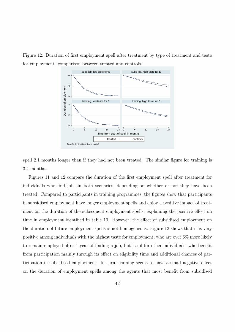
Figure 12: Duration of first employment spell after treatment by type of treatment and taste
for employment: comparison between treated and controls0
.51
0.5
1
0 6 12 18 24 0 6 12 18 24
subs job, low taste for E subs job, high taste for E
training, low taste for E training, high taste for E
treated controls
Dur
atio
n of
em
ploy
men
t
time from start of spell in months
Graphs by treatment and tasteE
spell 2.1 months longer than if they had not been treated. The similar figure for training is
3.4 months.
Figures 11 and 12 compare the duration of the first employment spell after treatment for
individuals who find jobs in both scenarios, depending on whether or not they have been
treated. Compared to participants in training programmes, the figures show that participants
in subsidised employment have longer employment spells and enjoy a positive impact of treat-
ment on the duration of the subsequent employment spells, explaining the positive effect on
time in employment identified in table 10. However, the effect of subsidised employment on
the duration of future employment spells is not homogeneous. Figure 12 shows that it is very
positive among individuals with the highest taste for employment, who are over 6% more likely
to remain employed after 1 year of finding a job, but is nil for other individuals, who benefit
from participation mainly through its effect on eligibility time and additional chances of par-
ticipation in subsidised employment. In turn, training seems to have a small negative effect
on the duration of employment spells among the agents that most benefit from subsidised
42

employment. Driving this effect are the zero returns to productivity of training and the higher
value of unemployment due to renewed eligibility to unemployment insurance.
4.5 Average effects of treatment on the treated: observed charac-
teristics
The results above show that the impact of treatment is heterogeneous and selection on unob-
served gains is important (although not so much for subsidised employment, perhaps because
it is in such low offer). However, these are not very useful for the policy maker, who cannot
observe unobservable types, and therefore cannot use this information to target interventions
more effectively. We now discuss how selection and treatment effects vary with observable
characteristics.
Table 13: Selection into treatment by observable characteristics - proportion of treated in
group
% in subsidised employment % in training
By experience at inflow
(1) lowest quartile 2.7% 18.7%
(2) 2nd quartile 2.4% 16.3%
(3) 3rd quartile 1.9% 14.6%
(4) highest quartile 1.6% 13.1%
By duration of unemployment up to enrolment
(5) less than 5 months 1.4% 9.8%
(6) 6 to 12 months 11.7% 88.3%
(7) over 12 months 8.6% 91.1%
Total 2.2% 15.7%
43
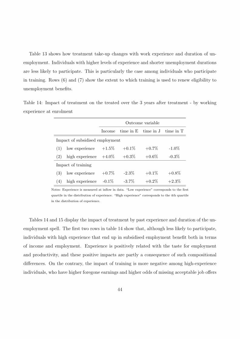
Table 13 shows how treatment take-up changes with work experience and duration of un-
employment. Individuals with higher levels of experience and shorter unemployment durations
are less likely to participate. This is particularly the case among individuals who participate
in training. Rows (6) and (7) show the extent to which training is used to renew eligibility to
unemployment benefits.
Table 14: Impact of treatment on the treated over the 3 years after treatment - by working
experience at enrolment
Outcome variable
Income time in E time in J time in T
Impact of subsidised employment
(1) low experience +1.5% +0.1% +0.7% -1.0%
(2) high experience +4.0% +0.3% +0.6% -0.3%
Impact of training
(3) low experience +0.7% -2.3% +0.1% +0.8%
(4) high experience -0.1% -3.7% +0.2% +2.3%
Notes: Experience is measured at inflow in data. “Low experience” corresponds to the first
quartile in the distribution of experience. “High experience” corresponds to the 4th quartile
in the distribution of experience.
Tables 14 and 15 display the impact of treatment by past experience and duration of the un-
employment spell. The first two rows in table 14 show that, although less likely to participate,
individuals with high experience that end up in subsidised employment benefit both in terms
of income and employment. Experience is positively related with the taste for employment
and productivity, and these positive impacts are partly a consequence of such compositional
differences. On the contrary, the impact of training is more negative among high-experience
individuals, who have higher foregone earnings and higher odds of missing acceptable job offers
44
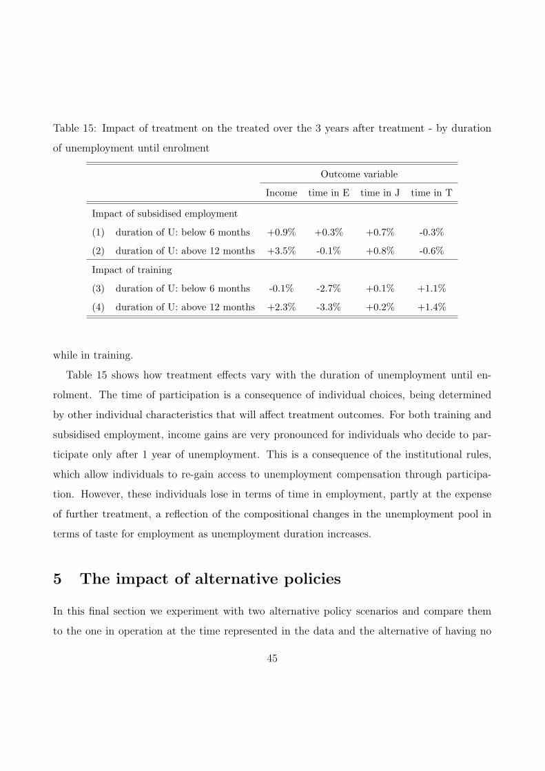
Table 15: Impact of treatment on the treated over the 3 years after treatment - by duration
of unemployment until enrolment
Outcome variable
Income time in E time in J time in T
Impact of subsidised employment
(1) duration of U: below 6 months +0.9% +0.3% +0.7% -0.3%
(2) duration of U: above 12 months +3.5% -0.1% +0.8% -0.6%
Impact of training
(3) duration of U: below 6 months -0.1% -2.7% +0.1% +1.1%
(4) duration of U: above 12 months +2.3% -3.3% +0.2% +1.4%
while in training.
Table 15 shows how treatment effects vary with the duration of unemployment until en-
rolment. The time of participation is a consequence of individual choices, being determined
by other individual characteristics that will affect treatment outcomes. For both training and
subsidised employment, income gains are very pronounced for individuals who decide to par-
ticipate only after 1 year of unemployment. This is a consequence of the institutional rules,
which allow individuals to re-gain access to unemployment compensation through participa-
tion. However, these individuals lose in terms of time in employment, partly at the expense
of further treatment, a reflection of the compositional changes in the unemployment pool in
terms of taste for employment as unemployment duration increases.
5 The impact of alternative policies
In this final section we experiment with two alternative policy scenarios and compare them
to the one in operation at the time represented in the data and the alternative of having no
45

available treatments while unemployed.
The first policy alternative (policy 1 ) removes the link between UI eligibility and programme
participation. In this case, only regular employment can allow one to regain access to fully
subsidised unemployment. This policy scenario reproduces the design introduced in February
2001.
The second policy alternative (policy 2 ) sanctions the refusal to participate in an offered
treatment by cutting eligibility to unemployment compensation until the individual regains
eligibility through treatment or employment. While refusal to take up adequate treatment or
employment is sanctioned in Sweden, this seems to happen only on the paper, being seldom
used in practiced. In this policy scenario we enquire what would happen if treatment were to
become compulsory as has been implemented in other countries such as the UK with the New
Deal for Young People.
We denote by baseline the scenario where no treatment is available and by current policy the
scenario used in estimation characterised by both treatments being available, the possibility
to renew eligibility through treatment and the absence of sanctions.
In all this analysis we are abstracting from potential indirect effects. This is a reasonable
assumption if the policy affects a small proportion of individuals but is not as credible if we are
discussing large policy reforms. In particular, the transition from our baseline scenario to one
of the alternative policies could arguably involve important changes in the functioning of the
labour market that would change the parameters we take as structural. However, to study the
labour market responses to the change in policy scenarios is outside the scope of this paper.
Instead, our impacts can be understood at an individual level as if others would continue to
face the policy scenario used in estimation.
To construct the simulated data we use the initial distribution of observable characteristics
from the real data and simulate the labour market behaviour of these individuals for three years
from inflow. In all cases we compute the additional cost per capita of providing treatment as
46

compared to a baseline where only unemployment benefits are available. Our estimates of the
costs of unemployment include the income paid to individuals while out of work and the cost
of programmes as reported in Carling and Richardson (2004). We then simulate the effect
of the different scenarios on labour market outcomes under the assumption that the required
additional funding to support the alternative policies comes from sources other than the tax
payments of the target group.
Table 16: Effects of alternative policies on outcomes over the first 3 years after inflow
Effects of alternative policies
Current Policy 1: Policy 2:Baseline policy no renew sanction
(1) Time in unemployment 33.5% -1.05% -1.82% -4.63%
(2) Time in employment 66.5% -5.33% -3.69% -2.44%
(3) Utility 110.4(**) +1.33% +0.89% -2.62%
(4) Income 579.9(*) -0.53% -0.88% -5.18%
(5) Income from employment 447.4(*) -8.32% -5.77% -4.05%
(6) Gov’t expenditure 132.5(*) +31.45% +20.32% -2.91%
(*) Values are in 1000s SEK and per capita over the 3 years.
(**) Accumulated utility over the 3 years.
Table 16 shows how the three alternative policies compare with the scenario where no
treatment is available. All policies imply less unemployment and less employment, with the
difference being taken up by programmes. However, it is quite clear that in this respect the
policy that reduces employment most is the current policy. The removal of the link between
eligibility and the sanctions increase employment relative to the current policy.
Both the current policy and policy 1 have positive effects on the well-being of these individ-
uals (row (3)) despite the reduction in income (row (4)). The reduction in earnings (row (5))
is compensated by an increase in subsidies. The reason for the increase in welfare may be due
47

to the reduction in income volatility - our individuals are risk averse with a log utility.
Row (6) displays the change in government costs to support the change in policy. These
include direct costs of unemployment benefits and the provision of treatment but not changes
in revenue due to changes in employment choices and, therefore, in income tax revenue. The
second and third columns in row (6) show that making treatment available is very expensive,
increasing expenditure on unemployment compensation and the provision of treatment by up
to 30% (the impact would be even more negative if we account for losses in revenue due to
decreased taxable income). However, excluding the possibility of renewing eligibility through
programme participation allows for important savings as compared with the current policy,
and does so without substantially affecting wellbeing or income.
The introduction of sanctions reduces utility and income much more dramatically because it
induces very short subsidised unemployment spells. Employment income is higher relative to
the other two policy alternatives. As a consequence of the substantial reductions in transfers
to the unemployed, the introduction of sanctions could actually lead to government savings as
compared to the baseline scenario. This, however, is at the expense of large losses in welfare
and income for this group.
Figure 13 shows that the reduction in employment probabilities due to the availability of
treatment is persistent over time, particularly for the current policy and policy 1. Out-of-work
probabilities under policy 2 seem to catch up with those of the baseline as unemployment
becomes much less attractive under this policy. The strong penalty that sanctions impose on
unemployment is confirmed in figure 14, which shows that policy 2 is the only one to positively
affect the duration of employment as compared to the baseline.
48
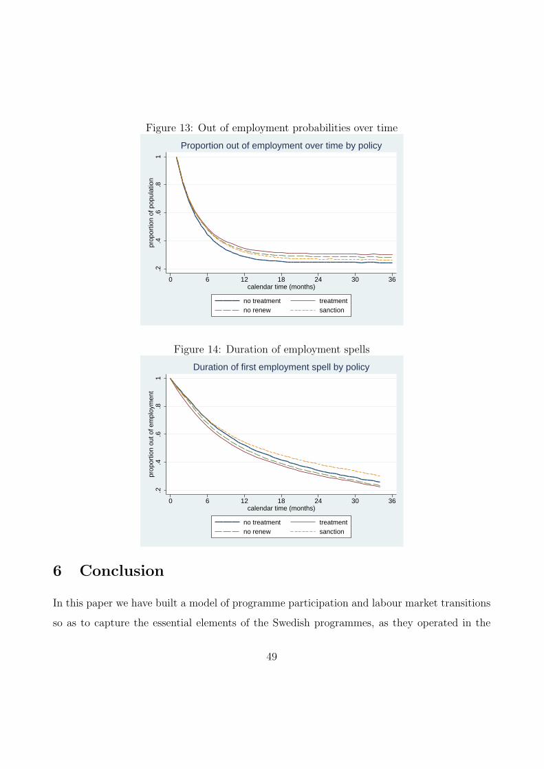
Figure 13: Out of employment probabilities over time
.2.4
.6.8
1pr
opor
tion
of p
opul
atio
n
0 6 12 18 24 30 36calendar time (months)
no treatment treatmentno renew sanction
Proportion out of employment over time by policy
Figure 14: Duration of employment spells
.2.4
.6.8
1pr
opor
tion
out o
f em
ploy
men
t
0 6 12 18 24 30 36calendar time (months)
no treatment treatmentno renew sanction
Duration of first employment spell by policy
6 Conclusion
In this paper we have built a model of programme participation and labour market transitions
so as to capture the essential elements of the Swedish programmes, as they operated in the
49

mid to late 90s. Our model also accounts for UI eligibility and how this relates both to work
and programme spells. Contrary to earlier evaluations, our model captures the important dy-
namic interactions and considers both short term and longer term outcomes including earnings.
Questions we consider include the effectiveness of job training programmes and subsidised job
placements in reducing unemployment, improving job attachment and increasing earnings. To
achieve this we model transitions between unemployment, programmes and work, jointly with
earnings, for a cohort of individuals who became unemployed in 1996. The model is of the
dynamic, discrete choice, forward-looking type and is estimated for the population of unskilled
males aged 26 to 30 who have a period of unemployment starting during 1996. We use rich
administrative data which have been put together for this purpose.
Our results are sobering. The current policy reduces employment quite substantially by
increasing programme participation (including subsidised jobs). There is practically no effect
on earnings - training leaves them unchanged, while a spell in subsidised employment has a
third of the effect on earnings than does a normal job. However the current policy, despite the
decline in income, does seem to increase welfare; the reason for this is likely to be the reduction
in income volatility.
A substantial improvement over the current policy is obtained if programmes cannot be used
to renew eligibility for unemployment insurance: while the positive welfare gains are maintained
there is a substantial increase in employment, relative to the current policy. Further increases
in employment, but this time at the expense of a decline in overall welfare for this group, can
be achieved by imposing sanctions on those who refuse to participate in a programme.
The results seem to show that the programme component of the Swedish active labour
market system is at best a costly and ineffective approach. The insurance element of the
system seems important for welfare purposes. The large costs of the programmes would seem
to be better spent on other interventions. One element of the programmes that could perhaps
be thought useful are subsidised placements. So if anything, the training component should
50
be reduced and the subsidy programmes expanded.
Appendix A: Estimates
Tables 17 and 18 present the full set of estimated parameter of the model together with the
respective standard errors.
Appendix B: Likelihood function
The contribution to the likelihood of each type of transition conditional on unobserved het-
erogeneity is described below. In the end, we set up the overall likelihood function.
Let V Eit be the present value of the employment option for individual i at time t excluding
the contemporary transitory taste shock. Thus, V Eit = V E
it − εEit . Similarly define V J
it = V Jit − εJ
it
and V Tit = V T
it − εTit. For ease of notation, we omit the arguments from the value functions in
what follows, namely (Ωit, Γit, θi) as defined in the main text. However, for clarity we include
the productivity shock when relevant. Finally, let Lit(l, l′) be the contribution to the likelihood
a transition from activity l to activity l′ observed between period t− 1 and t for individual i.
It may or may not include a model of earnings depending on the type of transitions. This is
made explicit in what follows.
Transitions from employment into employment
• No wage innovation occurs with probability 1 − π, in which case the wage in period t
is the same as in period t − 1 and the productivity shock, νit, is such that wit = wit−1.
Let V E be evaluated at such point and denote it by V Eit (νit : wit = wit−1). Then the
51
contribution to the likelihood function of such transitions and wage draw is
Lit(E, E) = g(d,w) (dit = E, wit|dit−1 = E, νit−1, Ωit, θi)
= (1− π)
[1− Φ
(V U
it − V Eit (νit : wit = wit−1)
σE
)]
where g(d,w) is the conditional joint density of present labour market activity and earnings
given the particular state space realisation.
• A wage innovation occurs then the new productivity shock ν is drawn from the distribu-
tion N (0, σ1). Let V E be evaluated at the drawn innovation and denote it by V Eit (νit).
Then the contribution to the likelihood function of such transition and wage draw is
Lit(E, E) = g(d,w) (dit = E, wit|dit−1 = E, Ωit, θi)
= π
[1− Φ
(V U
it − V Eit (νit)
σE
)]φ
(νit
σ1
)1
σ1
Transitions from employment into unemployment The contribution to the likelihood
in this case weights the two possibilities: having or not experienced a wage innovation. Using
the same notation as above we have
Lit(E, U) = gd (dit = U |dit−1 = E, νit−1, Ωit, θi)
= (1− π)Φ
(V U
it − V Eit (νit : wit = wit−1)
σE
)+
π
∫ +∞
−∞Φ
(V U
it − V Eit (ν)
σE
)φ
(ν
σ1
)1
σ1
dν
where gd is the conditional probability of the present labour market activity given the particular
state space realisation.
Transitions from subsidised employment into employment We assume there is always
an innovation in this case, which is consistent with the data. We use the same notation as
52

above. We also omit the arguments from the offer probabilities for simplicity of notation except
for the previous labour market status,
Lit(J,E) = g(d,w) (dit = E, wit|dit−1 = J, Ωit, θi)
= oEit (dit−1 = J)
[1− Φ
(V U
it − V Eit (νit)
σE
)]φ
(νit
σ1
)1
σ1
Transitions from subsidised employment into subsidised employment Again, there
are two possibilities depending on whether there is an innovation. However, there is never an
innovation in the data so we consider the case of no innovation only. We use a similar notation
to the explained above.
Lit(J, J) = g(d,w) (dit = J,wit|dit−1 = J, νit−1, Ωit, θi)
= oJit (dit−1 = J) (1− π)
[1− Φ
(V U
it − V Jit (νit : wit = wit−1)
σJ
)]
Transitions from subsidised employment into unemployment In this case we consider
the possibility of having or not received a wage innovation if another instance of subsidised
employment is offered (and rejected),
Lit(J, U) = gd (dit = U |dit−1 = J, νit−1, Ωit, θi)
= oEit (dit−1 = J)
∫ +∞
−∞Φ
(V U
it − V Eit (ν)
σE
)φ
(ν
σ1
)1
σ1
dν +
oJit (dit−1 = J) (1− π)Φ
(V U
it − V Jit (νit : wit = wit−1)
σJ
)+
oJit (dit−1 = J) π
∫ +∞
−∞Φ
(V U
it − V Jit (ν)
σJ
)φ
(ν
σ1
)1
σ1
dν +
[1− oE
it (dit−1 = J)− oJit (dit−1 = J)
]
Transitions from training or unemployment into employment Let l denote the labour
market status in period t− 1, either training T or unemployment U . In this case, transitions
53

to employment can only occur if there is an offer and this is a draw from the wage distribution
determined by the productivity shocks, which follow a distribution N (0, σ0). Transitions into
employment make the following contribution to the likelihood function,
Lit(l, E) = g(d,w) (dit = E, wit|dit−1 = l, Ωit, θi)
= oEit (dit−1 = l)
[1− Φ
(V U
it − V Eit (νit)
σE
)]φ
(νit
σ0
)1
σ0
Transitions from training or unemployment into subsidised employment Following
the same notation as above,
Lit(l, J) = g(d,w) (dit = J, wit|dit−1 = l, Ωit, θi)
= oJit (dit−1 = l)
[1− Φ
(V U
it − V Jit (νit)
σJ
)]φ
(νit
σ0
)1
σ0
Transitions from training or unemployment into training These are also conditional
on receiving an offer but no wage is drawn,
Lit(l, T ) = gd (dit = T |dit−1 = l, Ωit, θi)
= oTit (dit−1 = l)
[1− Φ
(V U
it − V Tit
σT
)]
54

Transitions from training or unemployment into unemployment Following the same
notation as before,
Lit(l, U) = g(d,w) (dit = U |dit−1 = l, Ωit, θi)
= oEit (dit−1 = l)
∫ +∞
−∞Φ
(V U
it − V Eit (ν)
σE
)φ
(ν
σ0
)1
σ0
dν +
oJit (dit−1 = l)
∫ +∞
−∞Φ
(V U
it − V Jit (ν)
σJ
)φ
(ν
σ0
)1
σ0
dν +
oTit (dit−1 = l) Φ
(V U
it − V Tit
σT
)+
[1− oE
it (dit−1 = l)− oJit (dit−1 = l)− oT
it (dit−1 = l)]
Overall likelihood The overall likelihood for the conditional sample of individuals entering
unemployment at time t = 1 is
L =N∏
i=1
∫
θ∈Θ
T∏t=2
∏
l,l′=U,E,J,T
Lit (l, l′)1(dit=l′,dit−1=l) ∗ fΩt|Ωt−1,dt−1,θ (Ωit|Ωit−1, dit−1, θ) ∗
fΩ1|d0,d1,θ (Ωi1|di0 = E, di1 = U, θ) ∗ fθ|d0,d1 (θ|di0 = E, di1 = U)
dθ
In the present case we consider a discrete distribution for the unobserved heterogene-
ity. This means that the integral in the above expression can be replace by a summation.
We also consider a deterministic evolution of the observable variables conditional on the
previous period information, so fΩt|Ωt−1,dt−1,θ (Ωit|Ωit−1, dit−1, θ) is excluded from the likeli-
hood function. At this stage we are also taking the initial conditions as exogeneous so that
fΩ1|d0,d1,θ (Ωi1|di0 = E, di1 = U, θ) is not included in the likelihood function. This will be relaxed
in future work. So the likelihood function simplifies to,
L =N∏
i=1
∑
θ∈Θ
T∏t=2
∏
l,l′=U,E,J,T
Lit (l, l′)1(dit=l′,dit−1=l)fθ|d0,d1 (θ|di0 = E, di1 = U)
55

Appendix C: Data
Data sources
The estimation of the structural model relies on the availability of a particularly rich data set,
which follows workers through a long period and allows one to link earnings information to
employment, programme and unemployment spells. We exploited a uniquely comprehensive
combination of both new and updated series of datasets. This involved linking the various
types of available information, summarised in Table C1, both over time (from January 1990 to
December 1998) and across labour market states (spells in education, employment, compen-
sated and uncompensated unemployment, programme participation and inactivity).
Unemployment and programme participation histories are provided by the various databases
of Handel, the unemployment register. This longitudinal event history dataset, available from
August 1991 to June 2000, has information on all unemployed individuals registered at the
public employment offices and provides labour market status information over time (e.g. un-
employed, on a given programme, temporarily employed), together with important personal
characteristics of the job-seeker and the reason for leaving the employment office (e.g. obtained
employment, gone on regular education or left the workforce).
Akstat, available from January 1994 to June 2000, originates from the unemployment in-
surance funds and provides information on spells of unemployment benefits, including the type
(UI or KAS where KAS is cash assistance and is unrelated to previous earnings) and amount
of compensation paid out.
Employment information by employment and calendar year is available from the Kontrolluppgifts-
registry from 1990 to 1998. This information is provided by each employer for tax purposes
and contains the first and last calendar months where the worker has been employed by that
employer as well as the corresponding employment income paid out to him during that period.
The highest educational qualification achieved within a given calendar year (1990 to 1998)
56

together with other demographic information is obtained from Statistics Sweden.
The end result is a very large and representative dataset, with information about the du-
ration of stay in a labour market state, employment earnings, an array of demographic and
human capital variables and, for entitled individuals, additional information on type of enti-
tlement, unemployment benefit recipiency and previous working conditions.
Data issues
Despite the comprehensiveness of the data, a number of important shortcomings had to be
dealt with to construct the dataset for analysis.
The first problem relates to the availability of information while out of the unemploy-
ment register (Handel). Handel is the most reliable data source but it contains no additional
information about individuals labour market status in between registration periods beyond
the initial state to which the individual moves upon leaving the office. Furthermore, the at-
trition/misclassification problem of individuals being recorded as having left simply because
“contact ended” means that we do not know whether they have found a job they did not
report, or are still in (unregistered) unemployment (cf. Bring and Carling, 2000, and Sianesi,
2004).
The employment information reported by employers has been used to fill in such gaps.
However, it is in itself not free of problems. First, employment spells recorded in the data
are not necessarily uninterrupted; we only know that an individual has been paid at least in
the first and last months recorded by that employer but we cannot ascertain for sure whether
the worker has been paid in the intermediate period unless he/she re-registers as unemployed
or participates in a programme. Second, and potentially more serious, is the occurrence of
employment spells with missing start and end dates and whose income is thus unallocated
over the calendar year. The incidence of such spells is low (2-3% of total spells) but they
affect 20% of our sample individuals. Based on a number of exploratory analysis, our preferred
57

procedure has been to spread these spells over the whole year for as long as the worker is
not reported as being in registered unemployment or on a programme. A third problem with
the employment data relates to the suspected over-reporting of January-to-December spells.
Again, these spells have been interrupted for eventual periods in registered unemployment or
on programmes.
We detect participation in education using outflows from registered unemployment into
education and from upgrades to the highest qualification. However, the incidence of missing
information for the “reason to leave registered unemployment” together with the fact that
educational data are censored at the end of 1998 (and therefore, ongoing investments cannot
be determined) imply that some upgrades and educational spells will be missed.
Once cleaned and merged, the data suffer from the following shortcomings:
• Low consistency of information from the various sources, in particular: (i) time in em-
ployment according to Handel and to the employer-provided data (10% of employment
spells in the latter are not compatible with unemployment or programme participation
reported in Handel); (ii) monthly income from Akstat and the one derived from the an-
nual payments reported by employers; (iii) highest educational attainment at the time of
registering as unemployed from Handel and in that calendar year from Statistics Sweden
(good correspondence at the compulsory and secondary levels, but not at the tertiary
one); and (iv) unemployment compensation according to Akstat and Handel (21% of
monthly spells where individuals receive compensation are not compatible with states
measured in Handel).
To deal with these inconsistencies, priority has been given to the most reliable data source
in a given case, and further decisions taken on the basis of exploratory and cross-checking
analyses which also involved the use of additional data sources (in particular, Louise and
education data from compulsory school Grundskola).
58

• Definition of an individual’s labour market state in a given month: it is not straight-
forward to reliably specify the state in which an individual is in a given month, this
being especially the case for education and employment, for which no monthly data is
available. Further conceptual issues relate to how to treat part-time employment whilst
registered at the unemployment office. Based on exploratory analysis (e.g. the income
they earn is substantial compared to income earned on other employment spells) and
the institutional treatment of part-time employment (which counts towards renewing
eligibility to UI just as full-time employment does), we have decided to treat part-time
employment as full-time employment. However, part-time employed workers do receive
unemployment compensation and have preferential access to programmes as compared
to deregistered individuals.
• Computation of monthly employment income: while employment income would be per-
fectly apportioned over a calendar year (confirmed also by the very good correspondence
between total employment income in that calendar year and income from the Louise
dataset), it is difficult to apportion employment income exactly over calendar months
due to the lack of reliable measures of the spell durations mentioned above.
Data preparation and set-up
Obvious mistakes giving rise to negative spells in Handel have been corrected and the re-
maining individuals with at least a negative spell have later been dropped from the sample
(this amounted to less than 4% of the original sample). Before being merged, the data has
been reshaped into calendar month history, taking the labour market state that lasted longest
in a month as the reference state for that month. The employer-provided data on employ-
ment spells has been corrected based on unemployment and programme spells information in
Handel. Monthly income from employment has then been calculated based on the corrected
59

employment spells and taking into account overlapping spells with different employers.
The following adjustments have also been made to set-up the data for estimating the model:
• Treatment spells: we only consider “long” programmes, i.e. those lasting more than
2 months. If a programme spell lasts 2 or fewer months, it is considered as time in
unemployment; if it lasts 3 months, one extra month on the programme is added; and
if it lasts more than 4 months, it is split up into shorter programme spells of 4 months
each.
• Direct employment-to-programme transitions: these occur in less than 0.2% of the transi-
tions on a monthly basis and are therefore prevented by including an intermediate period
in unemployment.
• Employment with no income: given the data limitations highlighted above, employment
is a residual category for when an individual is not registered as unemployed or taking
part in a programme. In terms of history before inflow, employment spells with no
corresponding income are set to unemployment; after inflow, employment or subsidised
employment spells with no corresponding income are censored from the moment the
individual enters the spell.
• Entitlement to unemployment insurance: over our analysis window, we consider individ-
uals as becoming eligible to 14 months of UI after being in employment or treatment for
4 months. The following variables have been created to capture these factors:
– Work experience: set to 0 in January 1990, experience is then calculated as the
cumulated number of months in employment till then.
– Months in employment or treatment to count towards renewing full eligibility: num-
ber of months in employment or treatment since the last time the individual has
started an unemployment spell being fully entitled to the 14 months of UI.
60

– Remaining months of UI eligibility: varies between 0 to 14 and is used up while in
unemployment.
Sample selection
The original dataset covered the population registering at an unemployment office between 1
August 1991 and 31 December 1998, with no occupational handicap and aged 16 to 30 (age
being defined as year of registering minus year of birth).
For our analysis we have selected the population of Swedish males registering at an unem-
ployment office during 1996 (note that from January 1996 individuals can no longer become
eligible to UI for the first time via a programme) as either full-time unemployed or to take
part in a programme. Individuals are then followed until December 1998, and their history
is known back to January 1990. Additionally, at the time of registering individuals had to
be aged 26-30 and have either compulsory education or 1-2 years of high school (60% of the
full inflow sample; educational attainment has been derived from Statistics Sweden under the
assumption that courses finish in May). The selected individuals are further observed not
to upgrade their educational level during the analysis window (representing over 93% of the
low-education individuals), never to have an occupational handicap (over 98% of original sam-
ple), never to be self-employed or sailors, never to have a negative spell (after corrections of
obvious mistakes, over 96% of the original sample), and never to be in programmes for older,
disabled or immigrant workers, in vocational rehabilitation or in self-employment grants. We
have further dropped from the sample individuals with UI at inflow but no compensation left
(less than 2%), as well as individuals not entitled to UI compensation at inflow but who fulfil
the eligibility criteria (20% of the sample).
61

References
[1] Bonjour, D., Dorsett, R., Kinght, G., Lissenburgh, S., Mukherjee, A., Payne, J., Range,
M., Urwin, P. and White, M. (2001), “New Deal for Young People: National Survey of
Participants, Stage 2”, Employment Service Report ESR67.
[2] Bring, J. and Carling, K. (2000), “Attrition and Misclassification of Drop-Outs in the
Analysis of Unemployment Duration”, Journal of Official Statistics, 4, 321-330.
[3] Carling, K. and Richardson K. (2004), “The relative efficiency of labor market programs:
Swedish experience from the 1990’s”, Labour Economics, 11(3), 335-54.
[4] Dorsett, R. (2006), “The new deal for young people: effect on the labour market status
of young men”, Labor Economics, 13(3), 405-22.
[5] Eckstein, Z. and Wolpin, K. (1989a), “Dynamic Labor Force Participation of Married
Women and Endogenous Work Experience”, Review of Economic Studies, 56(3), 375-90.
[6] Eckstein, Z. and Wolpin, K. (1989b), “The Specification and Estimation of Dynamic
Stochastic Discrete Choice Models: A Survey”, Journal of Human Resources, 24, 562-98.
[7] Forslund, A. and Krueger, A. (1997), “An Evaluation of the Swedish Active Labor Market
Policy: New and Received Wisdom”, in R. Freeman, R. Topel and B. Swedenborg (eds.),
The welfare state in transition, University of Chicago Press, 267-98.
[8] Greenberg, D., Ashworth, K., Cebulla, A. and Walker, R. (2004), “Do Welfare-to-Work
Programmes Work for Long?”, Fiscal Studies, 25, 27-53.
[9] Gregory, A. and Veale, M. (1985), ”Formulating Wald Tests of Non-Linear Restrictions”,
Econometrica, 53, 1465-1468.
62

[10] Ham, J. C. and LaLonde, R.J. (1996), “The Effect of Sample Selection and Initial Condi-
tions in Duration Models: Evidence from Experimental Data on Training”, Econometrica,
64, 175-205.
[11] Heckman, J., LaLonde, R.J. and Smith, J.A. (1999), “The Economics and Econometrics of
Active Labour Market Programs”, in Ashenfelter, O. and Card, D. (eds.), The Handbook
of Labour Economics, Volume III.
[12] Heckman, J. and Singer, B. (1984), “A Method for Minimizing the Impact of Distri-
butional Assumptions in Econometric Models for Duration Data”, Econometrica, 52(2),
271-320.
[13] Rust, J. (1994), “Structural Estimation of Markov Decision Processes” in Engle, R. and
McFadden, D. (eds.), Handbook of Econometrics, Volume 4, 30823139, North Holland.
[14] Sianesi, B. (2001a), “Swedish Active Labour Market Programmes in the 1990s: Overall
Effectiveness and Differential Performance”, Swedish Economic Policy Review, 8, 2, 133-
169.
[15] Sianesi, B. (2001b), “Differential Effects of Swedish Active Labour Market Programmes
for Unemployed Adults during the 1990s”, IFS working paper W01/25.
[16] Sianesi, B. (2004), “An Evaluation of the Swedish System of Active Labour Market Pro-
grammes in the 1990s”, Review of Economics and Statistics, 86, 1, 133-155.
63
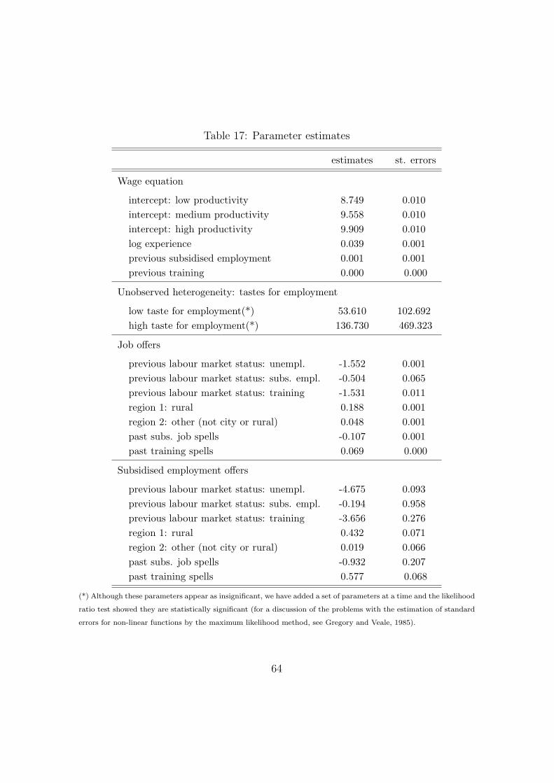
Table 17: Parameter estimates
estimates st. errors
Wage equation
intercept: low productivity 8.749 0.010intercept: medium productivity 9.558 0.010intercept: high productivity 9.909 0.010log experience 0.039 0.001previous subsidised employment 0.001 0.001previous training 0.000 0.000
Unobserved heterogeneity: tastes for employment
low taste for employment(*) 53.610 102.692high taste for employment(*) 136.730 469.323
Job offers
previous labour market status: unempl. -1.552 0.001previous labour market status: subs. empl. -0.504 0.065previous labour market status: training -1.531 0.011region 1: rural 0.188 0.001region 2: other (not city or rural) 0.048 0.001past subs. job spells -0.107 0.001past training spells 0.069 0.000
Subsidised employment offers
previous labour market status: unempl. -4.675 0.093previous labour market status: subs. empl. -0.194 0.958previous labour market status: training -3.656 0.276region 1: rural 0.432 0.071region 2: other (not city or rural) 0.019 0.066past subs. job spells -0.932 0.207past training spells 0.577 0.068
(*) Although these parameters appear as insignificant, we have added a set of parameters at a time and the likelihood
ratio test showed they are statistically significant (for a discussion of the problems with the estimation of standard
errors for non-linear functions by the maximum likelihood method, see Gregory and Veale, 1985).
64
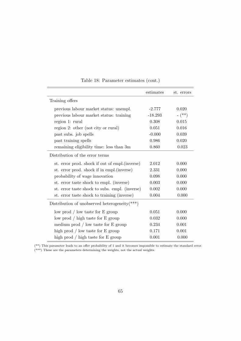
Table 18: Parameter estimates (cont.)
estimates st. errors
Training offers
previous labour market status: unempl. -2.777 0.020previous labour market status: training -18.293 - (**)region 1: rural 0.308 0.015region 2: other (not city or rural) 0.051 0.016past subs. job spells -0.000 0.039past training spells 0.986 0.020remaining eligibility time: less than 3m 0.860 0.023
Distribution of the error terms
st. error prod. shock if out of empl.(inverse) 2.012 0.000st. error prod. shock if in empl.(inverse) 2.331 0.000probability of wage innovation 0.098 0.000st. error taste shock to empl. (inverse) 0.003 0.000st. error taste shock to subs. empl. (inverse) 0.002 0.000st. error taste shock to training (inverse) 0.004 0.000
Distribution of unobserved heterogeneity(***)
low prod / low taste for E group 0.051 0.000low prod / high taste for E group 0.032 0.000medium prod / low taste for E group 0.234 0.001high prod / low taste for E group 0.171 0.001high prod / high taste for E group 0.001 0.000
(**) This parameter leads to an offer probability of 1 and it becomes impossible to estimate the standard error.
(***) These are the parameters determining the weights, not the actual weights.
65


![British Columbia Labour Market Outlook 2010 - 2020 · Labour Market OutlookLabour Market Outlook British Columbia Labour Market Outlook: 2010-2020 [2] B.C. Labour Market Outlook,](https://img.pdfslide.us/doc/110x75/5e167e8e481eae63a43f8127/british-columbia-labour-market-outlook-2010-2020-labour-market-outlooklabour-market.jpg)