Labour flexibility and its effects on labour

productivity growth

Master thesis

Master of science in management of technology Faculty of Technology Policy and Management

Author:

Arnar Ingason a.ingason@student.tudelft.nl Student number: 4186087

Graduation committee:

Chairman: Dr. Alfred Kleinknecht First supervisor: Dr. Servaas Storm Second supervisor: Dr. Jan van den Berg Third supervisor: Dr. Adrie C.M. Dumaij

Date: May 2013

1

Abstract

This study examines the relationship between labour productivity growth and labour

flexibility in Schumpeter Mark I and Mark II industries, with a focus on numerical and

functional flexibility. Ordinary least square regressions were estimated using panel data from

Dutch firms covering the years 2003-2009. The results revealed a negative and significant

relationship between the use of temporary labour and growth of sales per employee as a

measure of labour productivity. A doubling of workers on temporary contracts leads to an up

to ten per cent decline of labour productivity growth. Functional flexibility had to be

excluded from the estimates due to very low numbers of observations in the database. The

results suggest that high use of temporary labour will hamper productivity growth within

firms regardless of their innovation regime.

2

Table of Contents Abstract ................................................................................................................................................... 1

List of graphs, figures and tables ............................................................................................................. 4

1. The problem .................................................................................................................................... 5

1.1. Introduction ............................................................................................................................. 5

1.2. Theoretical background ........................................................................................................... 6

1.2.1. Labour productivity and growth trends .......................................................................... 6

1.2.2. The Anglo-Saxon model ................................................................................................... 7

1.2.3. The Continental (Rhineland) model ................................................................................ 8

1.2.4. The labour market ........................................................................................................... 8

1.2.5. The innovation regimes ................................................................................................... 9

1.3. Problem statement ................................................................................................................ 10

1.4. The purpose of the research ................................................................................................. 11

1.5. The research question ........................................................................................................... 12

1.6. Relevance of the study .......................................................................................................... 12

1.7. The Data ................................................................................................................................ 13

1.8. The outline of the research ................................................................................................... 14

2. Literature review and hypotheses ................................................................................................. 15

2.1. Review of literature ............................................................................................................... 15

2.1.1. Labour productivity, flexibility and Verdoorn’s law ...................................................... 15

2.1.2. Innovation regimes and possible effects on labour productivity .................................. 22

2.2. Conceptual model ................................................................................................................. 26

3. Research design and methodology ............................................................................................... 27

3.1. Research design ..................................................................................................................... 27

3.2. Data collection ....................................................................................................................... 28

3.3. Operational definition of research variables ......................................................................... 30

4. Analysis of data and interpretation of results ............................................................................... 34

4.1. Descriptive analysis ............................................................................................................... 34

4.1.1. Labour productivity ....................................................................................................... 34

4.1.2. Labour productivity growth ........................................................................................... 35

4.1.3. External (numerical) flexibility ....................................................................................... 37

4.1.4. Internal (functional) flexibility ....................................................................................... 38

4.1.5. Sales growth (Verdoorn effect) ..................................................................................... 40

4.1.6. Sector dummies ............................................................................................................. 41

3

4.2. Multiple regression analysis .................................................................................................. 42

4.3. The models ............................................................................................................................ 44

4.3.1. Models 1-5 ..................................................................................................................... 45

4.3.2. Models 6 and 7 .............................................................................................................. 50

5. Discussion, summary, conclusion and recommendations ............................................................ 53

5.1. Discussion, summary and conclusion .................................................................................... 53

5.2. Recommendations................................................................................................................. 55

6. Limitations and further research ................................................................................................... 56

Bibliography ........................................................................................................................................... 57

Appendix A ........................................................................................................................................ 63

Appendix B ........................................................................................................................................ 64

Appendix C......................................................................................................................................... 65

Appendix D ........................................................................................................................................ 67

4

List of graphs, figures and tables

Graph 1: Labour productivity growth trend in the euro area .................................................... 5

Graph 2: Labour productivity growth trends in US .................................................................... 6

Graph 3: Difference in amount of observations with or without intermediary goods ........... 30

Graph 4: Number of participants in the first 14 industries ...................................................... 32

Graph 5: Amount of observations in different firm size groups .............................................. 33

Graph 6: Labour productivity without sales spent on acquisition of intermediate inputs

versus labour productivity with sales spent on acquisition of intermediate inputs ............... 64

Figure 1: The conceptual model ............................................................................................... 26

Table 1: Industry categorization according to SBI93 code ....................................................... 14

Table 2: Descriptive test for the prior labour productivity variable ........................................ 34

Table 3: Descriptive analysis of the variable labour productivity growth ............................... 36

Table 4: Descriptive analysis of % of temporary workers ........................................................ 37

Table 5: Descriptive analysis of labour turnover...................................................................... 38

Table 6: Descriptive analysis of the variable % of reallocated personnel................................ 39

Table 7: Descriptive analysis of the variable sales growth ...................................................... 40

Table 8: Sectors and the corresponding SBI93 codes .............................................................. 41

Table 9: OLS regression using only two variables .................................................................... 44

Table 10: The categorization of industries into Mark I and Mark II innovation regimes ........ 46

Table 11: Results from analysis of models 1-3 ......................................................................... 47

Table 12: Results from analysis of models 4 and 5 .................................................................. 49

Table 13: Results from analysis of models 6 and 7 .................................................................. 51

Table 14: Correlation table including the main variables ........................................................ 64

Table 15: Data gathered after 2008 excluded .......................................................................... 65

Table 16: Model including the internal reallocation variable .................................................. 66

Table 17: Overview of hypotheses, criterion and results ........................................................ 67

5

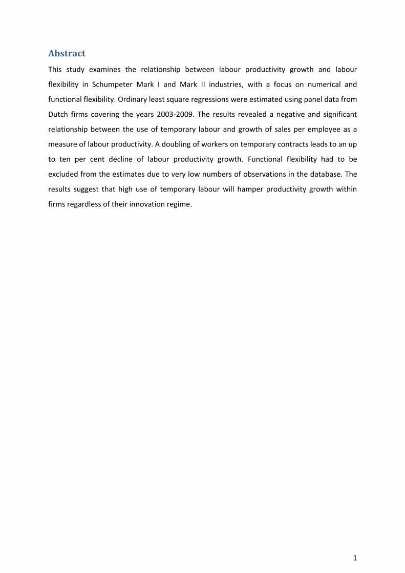
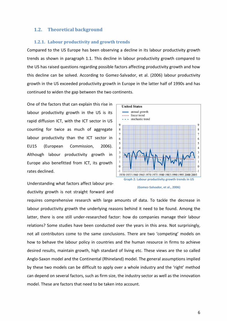
Graph 1: Labour productivity growth trend in the euro area

(Gomez-Salvador, et al., 2006)

1. The problem

1.1. Introduction

Throughout history the human being has strived towards increasing its stand, security and

welfare in society by all means possible. When the world was divided into many smaller

kingdoms the formula was simple: harvest crops and pay land taxes to your king. Today

though with the use of money instead of barter as a medium of exchange and increasing

globalization, what you do does just as much matter as what all others are doing. And the

fact that the global economy is not a zero-sum game if someone is doing much better than

you (in producing goods and services etc.) you lose your competitiveness and eventually you

go bankrupt and thus lose your stand, security and future welfare in the society. Therefore

doing better and thus stay competitive is an essential matter of survival, not only for

individuals and firms but for the society as a whole and to do that firms need to be

productive and utilize their resources as efficiently as possible.

Today the decrease in labour productivity

growth and their effects on the welfare of

societies are increasingly getting attention

from governments and firms around the

world as it has been declining1 in Europe

since the 1950s (Gomez-Salvador, et al.,

2006) as can be seen in graph 1.

One of firms’ most important factors is their

labour productivity. For staying competitive

and survive in the global market keeping it

high and growing is vital. Labour productivity is not only important at micro level, it is also

one of the key drivers for economic performance and it directly affects the welfare of

societies as a whole. It increases and maintains the standard of living and keeps countries in

the forefront of global performance (OECD, 2011).

1 The labour productivity growth has been declining as can be seen in chart 1 even though the labour

productivity itself has been increasing (Gomez-Salvador, et al., 2006). The labour productivity growth is the change in labour productivity (value added divided by labour units) from time t to t+1.

6

1.2. Theoretical background

1.2.1. Labour productivity and growth trends

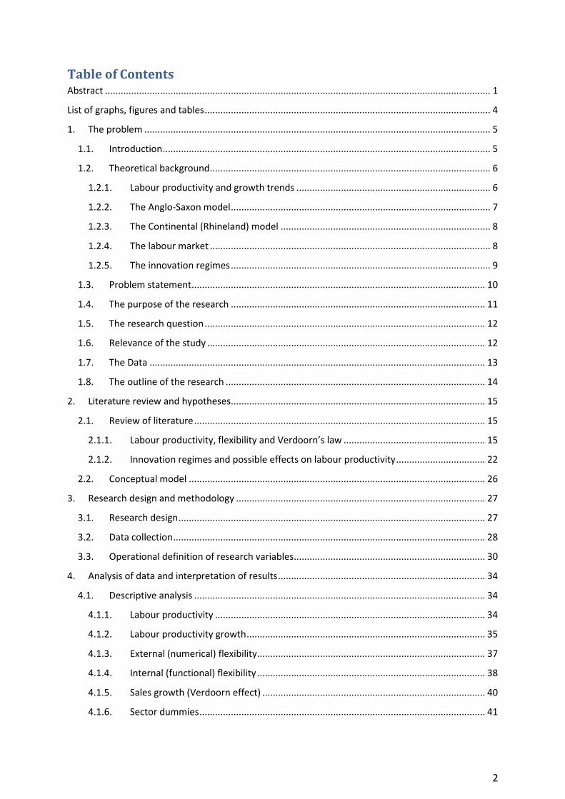
Compared to the US Europe has been observing a decline in its labour productivity growth

trends as shown in paragraph 1.1. This decline in labour productivity growth compared to

the US has raised questions regarding possible factors affecting productivity growth and how

this decline can be solved. According to Gomez-Salvador, et al. (2006) labour productivity

growth in the US exceeded productivity growth in Europe in the latter half of 1990s and has

continued to widen the gap between the two continents.

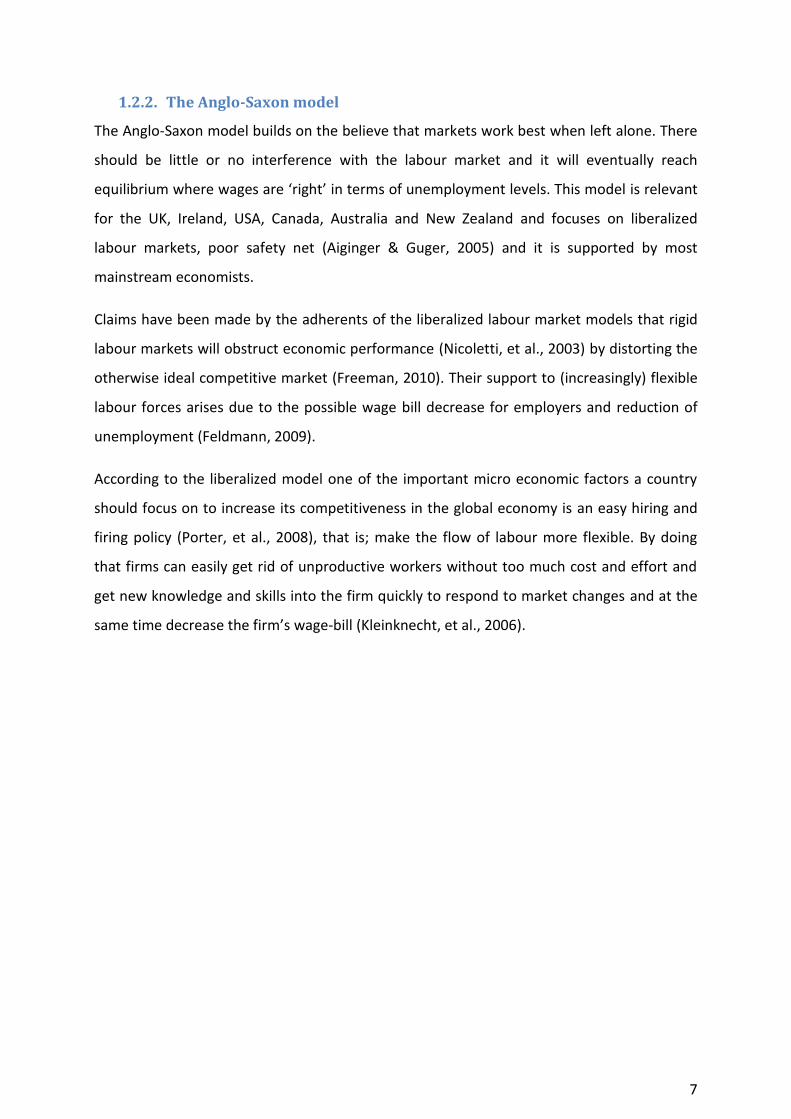
One of the factors that can explain this rise in

labour productivity growth in the US is its

rapid diffusion ICT, with the ICT sector in US

counting for twice as much of aggregate

labour productivity than the ICT sector in

EU15 (European Commission, 2006).

Although labour productivity growth in

Europe also benefitted from ICT, its growth

rates declined.

Understanding what factors affect labour pro-

ductivity growth is not straight forward and

requires comprehensive research with large amounts of data. To tackle the decrease in

labour productivity growth the underlying reasons behind it need to be found. Among the

latter, there is one still under-researched factor: how do companies manage their labour

relations? Some studies have been conducted over the years in this area. Not surprisingly,

not all contributors come to the same conclusions. There are two ‘competing’ models on

how to behave the labour policy in countries and the human resource in firms to achieve

desired results, maintain growth, high standard of living etc. These views are the so called

Anglo-Saxon model and the Continental (Rhineland) model. The general assumptions implied

by these two models can be difficult to apply over a whole industry and the ‘right’ method

can depend on several factors, such as firm size, the industry sector as well as the innovation

model. These are factors that need to be taken into account.

Graph 2: Labour productivity growth trends in US

(Gomez-Salvador, et al., 2006)

7

1.2.2. The Anglo-Saxon model

The Anglo-Saxon model builds on the believe that markets work best when left alone. There

should be little or no interference with the labour market and it will eventually reach

equilibrium where wages are ‘right’ in terms of unemployment levels. This model is relevant

for the UK, Ireland, USA, Canada, Australia and New Zealand and focuses on liberalized

labour markets, poor safety net (Aiginger & Guger, 2005) and it is supported by most

mainstream economists.

Claims have been made by the adherents of the liberalized labour market models that rigid

labour markets will obstruct economic performance (Nicoletti, et al., 2003) by distorting the

otherwise ideal competitive market (Freeman, 2010). Their support to (increasingly) flexible

labour forces arises due to the possible wage bill decrease for employers and reduction of

unemployment (Feldmann, 2009).

According to the liberalized model one of the important micro economic factors a country

should focus on to increase its competitiveness in the global economy is an easy hiring and

firing policy (Porter, et al., 2008), that is; make the flow of labour more flexible. By doing

that firms can easily get rid of unproductive workers without too much cost and effort and

get new knowledge and skills into the firm quickly to respond to market changes and at the

same time decrease the firm’s wage-bill (Kleinknecht, et al., 2006).

8

1.2.3. The Continental (Rhineland) model

Recently a number of studies from heterodox economists opposes the mainstream

economic view that rigidity of labour markets is bad and hampers labour productivity

growth. The heterodox economists defend more rigid labour markets and thus instead

support stronger labour relations, saying that stronger labour relations will in fact increase

labour productivity growth (Dekker & Kleinknecht, 2011) in firms and this again increases the

firms’ business success (Demeter, et al., 2010).

These studies have also shown that there is a negative relation between externally flexible

labour and labour productivity growth (Kleinknecht, et al., 2006). Recent studies suggest that

the relation between labour flexibility (internal and external) and labour productivity growth

may be moderated by whether the firms fall under the Schumpeter Mark I or Schumpeter

Mark II innovation model (Dekker & Kleinknecht, 2011). The Continental model focuses on

strong labour relations with high commitment and possibility of reallocation of labour within

companies, on active labour unions that have a strong and legal power to protect their

people’s right, and on high social benefits for out of work personnel as well as protection

against easy firing.

The free-flow of labour has often been attached to the increase globalization but Agell

(1999) came to the conclusion, by looking at data from the OECD countries, that increased

globalization of economic activities can lead to increase in the demand for different labour

market rigidities.

1.2.4. The labour market

The two models, Anglo-Saxon and the Continental model discussed above, both focus on

how to organize the labour market and it is divided into two main categories.

i) External (numerical) labour flexibility

External (numerical) labour flexibility involves focusing on easy hiring and firing of personnel

as the main target (Porter, et al., 2008). The use of externally flexible labour policies involves

high labour turnover, high shares of temporary workers and workers from labour force

agencies, weak labour unions and low social benefits for unemployed personnel

(Kleinknecht, 2011). Some of the heterodox economists’ argue against the external labour

9

flexibility policy implemented in the Anglo-Saxon model saying it may lead to a reduction of

trust between employees and the employer (Kleinknecht, et al., 2006).

As mentioned above, one of the factors adherents to increased external labour flexibility aim

at is the possible effect of decreasing the firms wage bill. Focusing on the firms’ wage bill

however seems more relevant in the short-term. What firms need to focus on are the

actions for long-term results. Having a high labour turnover will indeed decrease the wage

bill but the high turnover can result in leakage of firm specific knowledge and tacit

knowledge amongst employees (Kleinknecht, et al., 2006).

ii) Internal (functional) labour flexibility

While external (numerical) labour flexibility focuses on easing the flow of labour with as little

constraints as possible the internal (functional) flexibility focuses in steering the flow,

increase workers safety and the reallocation/movement of personnel within companies. In

other words, internal labour flexibility promotes mobility, adaptability and movement within

a firm, both horizontal and vertical movement (Qian, et al., 2012).

Heterodox economists argue that the reallocation of personnel within the company would

then increase employees’ commitment to the firm and their willingness to learn and use

their full potential for the firm (Kleinknecht, et al., 2006). This could result in reduction of

possible tacit knowledge leakage and maintain high level of firm specific expertise and thus

reduce the cost of training and educating large amounts of new personnel. Mainstream

economists however argue that too strict labour policies will obstruct possible growth of the

firms because getting new talent into the firma and get rid of unproductive workers will be

too hard and expensive.

1.2.5. The innovation regimes

In the modern world with ever increasing technology development firms need to be alert for

changes in the industry and be ready to adapt and implement new technologies through

continuous innovation processes. Successful innovation within companies keeps them

competitive by allowing them to acquire first mover’s advantages and reap high profits

(Mohr, et al., 2009).

Increasingly studies are being done to examine the possible mediating effects of the

innovation model firms follow on labour productivity growth under different labour

10

flexibility policies. There are two definitions of different innovation regimes in industry

explained by Austrian American economist Joseph Alois Schumpeter. The first one referred

to as Schumpeter Mark I and the latter as Schumpeter Mark II.

i) Schumpeter Mark I industries are characterized by low entry barriers in form of

cost and or technology. They consist of entrepreneurs and firms participating in

innovative activities and are characterized by creative destruction (Breschi, et al.,

2000). These industries are faced with high competition and lower levels of

concentration (Nelson & Winter, 1978).

ii) The Schumpeter Mark II on the other hand is characterized by creative

accumulation, large entry barriers and large established firms that make it difficult

for new innovators to enter the market (Breschi, et al., 2000). These industries are

often characterized by more advanced sciences (Keklik, 2003), oligopolistic

industries and are thus more concentrated.

The innovation regime a firm is located in can have a significant importance on how to

manage the human resources in the firm regarding the innovative success of the firm

(Martínez-Sánchez, et al., 2011) and therefore distinguishing between firms’ industry

characterizations can be helpful when examining the relationship between (internal and/or

external) labour flexibility and labour productivity growth.

1.3. Problem statement

Even with the increase in studies regarding labour productivity growth and the possible

factors contributing to its changes there has no consensus been reach that could explain the

changing trend in labour productivity growth. There most certainly is more than one factor

having an impact but one of the most debated ones is how to manage labour force with

regard to its flexibility. Should a free flow of labour with easy hiring and firing be even

increased with less regulation or should it be more rigid to protect labour and prevent easy

hiring and firing policies? It all depends on what the goal is. What do we want to achieve? Do

we want to increase wages, decrease unemployment or is the ultimate goal to increase

firms’ productivity growth and make our economy sustainable and competitive?

11

The problem to be addressed in this research is labour productivity growth, specifically the

decline of it recently, and how does flexibility of the labour force affect it?

Firms are different in structure and that needs to be taken into account when assessing a

problem facing the economy as a whole. Therefore, when assessing the problem of declining

labour productivity growth looking at labour flexibility alone is not sufficient. Other factors

as mentioned above, such as firm size, what industry the firms are in, the innovation model

they follow and output generation need to be examined also to effectively examine the

problem.

By searching for a relationship between labour productivity growth and the flow of the

labour force the hope is to shed light on how firms can manage their labour relations to

increase the firms’ labour productivity growth and therefore increase their competitiveness

in the global economy. The fact that the global economy is opening up even more with

emerging markets and cheap work forces in Asia, South-America as well as Africa makes the

decline in labour productivity growth in Europe an important issue to solve quickly and

effectively.

The increased involvement of the emerging markets in the world trade of manufacturing

goods has and increasingly will have implications on the competitiveness amongst countries

in Europe, North-America and all other OECD countries (OECD, 2002). Therefore the problem

of declining labour productivity growth is of most importance and needs to be addressed to

maintain Europe’s stand as a global leader in the forefront of economic activities.

1.4. The purpose of the research

The purpose of this research is to deepen the knowledge on factors affecting labour

productivity growth within firms in a market orientated economy and hopefully then find

key drivers and how they can be manipulated to improve labour productivity growth within

firms. Also the difference in effects regarding firms’ industry status as well as the innovation

regime they fall under, that is Schumpeter Mark I or Mark II, specifically;

The objective of this research is to investigate the significance of labour flexibility and how

the flexibility affects labour productivity growth in market orientated firm’s following

either Schumpeter Mark I or Mark II innovation models.

12

1.5. The research question

To be able to realize the research objective laid out above a relevant research question

needs to be answered. The following main research question has been formulated and put

forward:

What factors affect firms’ labour productivity growth in market orientated firms that can

be characterized as either Schumpeter Mark I or Schumpeter Mark II firms?

The question above is in quite general form and there are several interesting factors that

possibly work together in affecting the labour productivity growth. Therefore the research

question above can be broken into two sub-questions;

I. How and to what extent does internal (functional) labour flexibility affect firms’

labour productivity growth?

II. How and to what extent does external (numerical) labour flexibility affect firms’

labour productivity growth?

By answering these questions the objective should be realized and be a valuable input into

the current literature and knowledge in the field.

1.6. Relevance of the study

Today with increased global flow of workforces, more specialized jobs and increased

competition in the global economy being productive is an essential element for all firms to

stay competitive and excel in their field. Even though in recent decades the technology has

improved the productivity of most firms implementing automotive machinery, ICT etc. many

firms still rely to a large extent on the human labour force. The larger part of costs carried by

most firms is in its payment to employees in exchange for their work. It is therefore very

important for firms to understand the underlying reasons in their human resource

management that affects the firm’s productivity to increase ‘value for the money’ spent on

its labour.

Understanding the effects of flexible labour not only benefits firms but the society as a

whole. It can give an idea on how to generate labour policies within economies to sustain

13

and further increase countries’ social level, standard of living and general economic welfare.

The importance of implementing the ‘right’ policies is highly relevant and connected to how

firms manage their human resource management.

This research is not intended to solve the problem on its own, rather to serve as a valuable

input into the current scientific literature and together with the increasing knowledge gained

by similar research shed a light on ‘best’ practices to take, both on a societal level and firm

level.

1.7. The Data

The data to be used in this research are gathered from the Dutch Organization for Strategic

Labour Market Research 2 (OSA) that in 2010 was taken over by the Netherlands Office for

Social Research. OSA has conducted surveys every other year since 1989 for the purpose of

gathering data about Dutch firms. The survey consists of more than 500 questions and

around 3000 firms participate in the survey every other year. Not all firms participate in

every survey, some fall out due to bankruptcy, merger and acquisitions or simply do not

respond.

Each survey consists of telephone interviews as well as a written questionnaire. The

telephone interviews are three in total and the written questionnaire is only once and these

data are gathered on odd years and published on even years. The surveys have undergone

some changes during the course of time, new questions were added, and questions taken

out or reframed. Due to these changes data published in the years 2004-2010 (gathered in

2003-2009), total of 4 survey waves, will be used as in this time frame while the questions

remained the same.

The questions answered by the firms in the sample include general firm information,

financial and investment information, innovation, R&D expenditures and more. All the firms

are assigned a unique company number as well as a specific industry number called SBI3

code. In table 1 a broad list of different industries and their SBI codes can be seen.

2 Organisatie voor Strategisch Arbeidsmarktonderzoek (OSA)

3 The SBI (Standaard Bedrijfsindeling/Standard Industrial Classification) code is a coding procedure to

categorize firms according to their main activities in the market. The codes in the surveys were in accordance to the codes from 1993, SBI93.

14

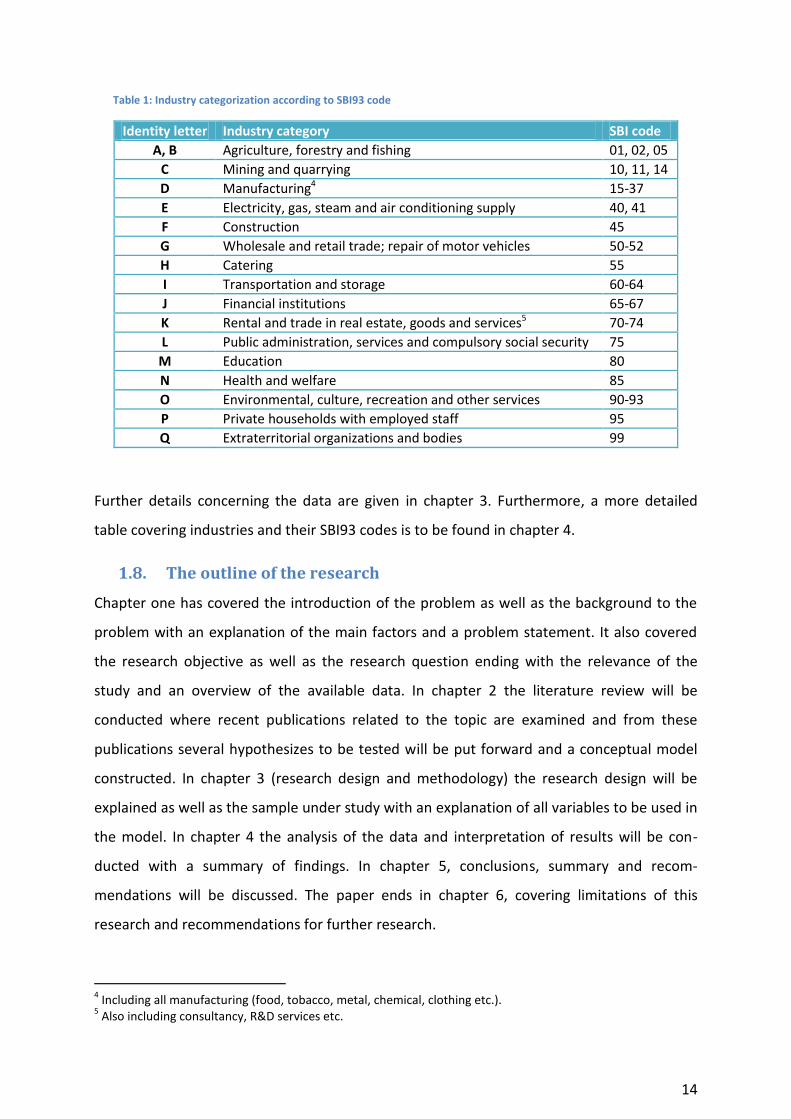
Table 1: Industry categorization according to SBI93 code

Identity letter Industry category SBI code

A, B Agriculture, forestry and fishing 01, 02, 05

C Mining and quarrying 10, 11, 14

D Manufacturing4 15-37

E Electricity, gas, steam and air conditioning supply 40, 41

F Construction 45

G Wholesale and retail trade; repair of motor vehicles 50-52

H Catering 55

I Transportation and storage 60-64

J Financial institutions 65-67

K Rental and trade in real estate, goods and services5 70-74

L Public administration, services and compulsory social security 75

M Education 80

N Health and welfare 85

O Environmental, culture, recreation and other services 90-93

P Private households with employed staff 95

Q Extraterritorial organizations and bodies 99

Further details concerning the data are given in chapter 3. Furthermore, a more detailed

table covering industries and their SBI93 codes is to be found in chapter 4.

1.8. The outline of the research

Chapter one has covered the introduction of the problem as well as the background to the

problem with an explanation of the main factors and a problem statement. It also covered

the research objective as well as the research question ending with the relevance of the

study and an overview of the available data. In chapter 2 the literature review will be

conducted where recent publications related to the topic are examined and from these

publications several hypothesizes to be tested will be put forward and a conceptual model

constructed. In chapter 3 (research design and methodology) the research design will be

explained as well as the sample under study with an explanation of all variables to be used in

the model. In chapter 4 the analysis of the data and interpretation of results will be con-

ducted with a summary of findings. In chapter 5, conclusions, summary and recom-

mendations will be discussed. The paper ends in chapter 6, covering limitations of this

research and recommendations for further research.

4 Including all manufacturing (food, tobacco, metal, chemical, clothing etc.).

5 Also including consultancy, R&D services etc.

15

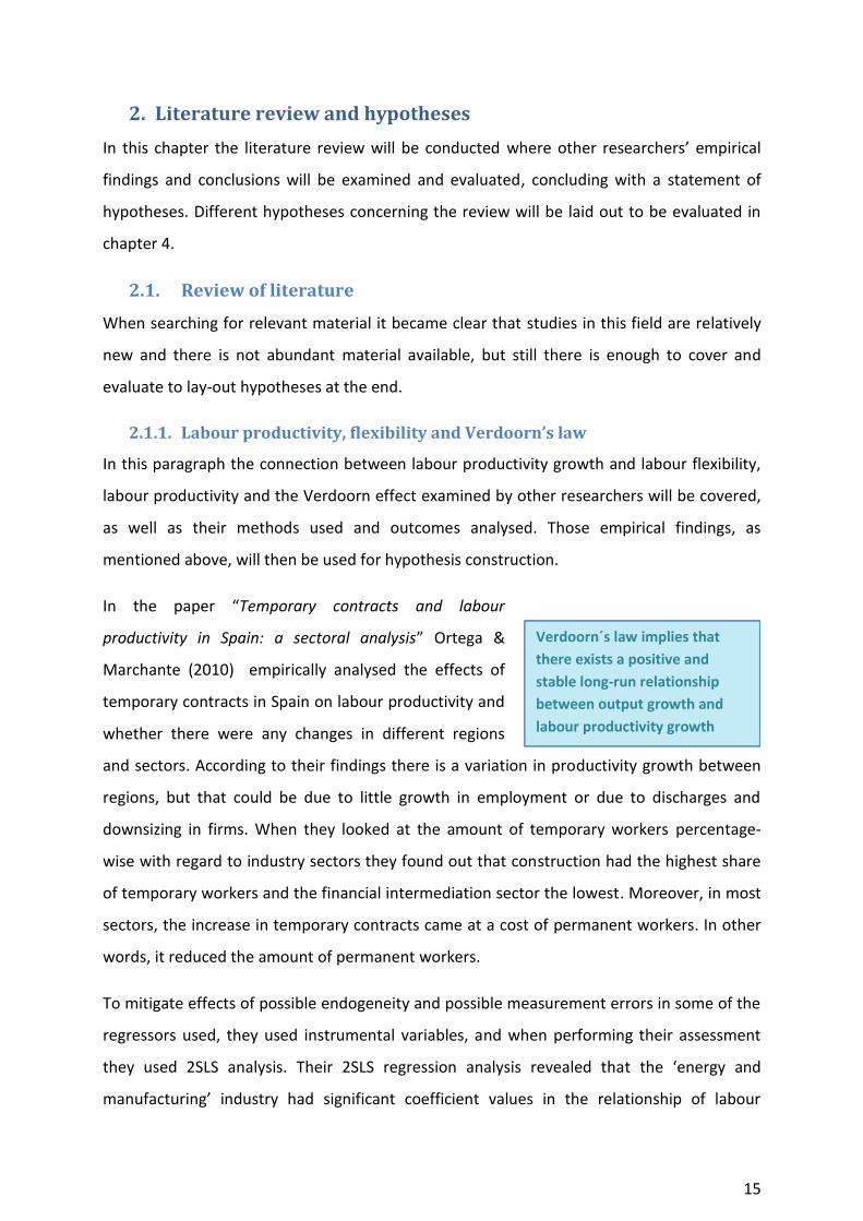
Verdoorn´s law implies that

there exists a positive and

stable long-run relationship

between output growth and

labour productivity growth

2. Literature review and hypotheses

In this chapter the literature review will be conducted where other researchers’ empirical

findings and conclusions will be examined and evaluated, concluding with a statement of

hypotheses. Different hypotheses concerning the review will be laid out to be evaluated in

chapter 4.

2.1. Review of literature

When searching for relevant material it became clear that studies in this field are relatively

new and there is not abundant material available, but still there is enough to cover and

evaluate to lay-out hypotheses at the end.

2.1.1. Labour productivity, flexibility and Verdoorn’s law

In this paragraph the connection between labour productivity growth and labour flexibility,

labour productivity and the Verdoorn effect examined by other researchers will be covered,

as well as their methods used and outcomes analysed. Those empirical findings, as

mentioned above, will then be used for hypothesis construction.

In the paper “Temporary contracts and labour

productivity in Spain: a sectoral analysis” Ortega &

Marchante (2010) empirically analysed the effects of

temporary contracts in Spain on labour productivity and

whether there were any changes in different regions

and sectors. According to their findings there is a variation in productivity growth between

regions, but that could be due to little growth in employment or due to discharges and

downsizing in firms. When they looked at the amount of temporary workers percentage-

wise with regard to industry sectors they found out that construction had the highest share

of temporary workers and the financial intermediation sector the lowest. Moreover, in most

sectors, the increase in temporary contracts came at a cost of permanent workers. In other

words, it reduced the amount of permanent workers.

To mitigate effects of possible endogeneity and possible measurement errors in some of the

regressors used, they used instrumental variables, and when performing their assessment

they used 2SLS analysis. Their 2SLS regression analysis revealed that the ‘energy and

manufacturing’ industry had significant coefficient values in the relationship of labour

16

productivity and share of temporary workers. Likewise, when all industries are pooled

together, a decrease of 1 percentage point in the amount of temporary contracts would

involve an increase of 0.32 percentage points in the mean annual growth rate in labour

productivity. Ortega & Marchante end their paper by emphasizing the urge to change the

amount of temporary contracts in the Spanish industry, mainly in energy and manufacturing.

The research performed by Ortega & Marchante also indicates that there is a negative

relationship between temporary contracts and labour productivity growth. This further

strengthens the view that too much usage of temporary labour can hamper labour pro-

ductivity growth in firms.

Another analysis was made by Lucidi (2008) who empirically analysed the effects of external

labour flexibility on labour productivity growth using firm-level data from the Italian Institute

for Vocational Training. The data contain information about firms’ contractual arrangement

to its employees, gender type, qualification of staff as well as the amount of personnel on

different types of contracts. Also information concerning firms’ financial statements was

used in constructing relevant variables. Because the data were presented both in cross-

sectional as well as in longitudinal form Lucidi used a two-step estimation procedure. The

variables he used in his model concerned growth rate of labour productivity as well as the

growth rate of firms’ value added (Verdoorn law), labour cost growth rate relative to price of

machinery and growth rate for fixed capital per employee.

When assessing the effects of flexible labour on labour productivity growth he used the

following variables: share of fixed term contracts, share of contract workers, and share of

temporary help workers. He also divided these variables into 4 categories (dummy variables)

to mitigate for possible non-linearity of the variables. The results indicated a negative

relationship between fixed term contracts and labour productivity with the coefficient

magnitude at -0.63 percentage points. The share of temporary help workers also reveals a

statistically significant negative relationship with labour productivity with the coefficient

magnitude at -0.86 percentage points. Interestingly, the research revealed that the share of

contract workers was positively and significantly correlated to labour productivity growth.

According to Lucidi (2008) this could be due to the fact that many contract workers are

17

consultants and or expert workers, but the database used did not have the information

about education and expertise level to assess this kind of information.

When the variables were split into groups (low, medium and high) they revealed an

increased negative correlation with an increased share of fixed term workers, with the high

group (more than 20% of personnel with fixed term contracts) statistical significance at the

1% level. The contract workers showed an increased positive relationship after being divided

into groups, with the high group statistically significant at the 5% level. After dividing the

temporary help workers into groups none of them showed statistical significance, as was the

case before group division.

Lucidi also looked at the possible effect of firm size (measured by number of personnel) on

labour productivity growth, as well as the possible Verdoorn effect, and found that

increasing firm size corresponds to increased labour productivity. That could be because

large firms often benefit from scale economies. The Verdoorn effects also showed a positive

correlation with labour productivity growth indicating increasing returns at firm level.

The results Lucidi got from his analysis indicate as Ortega & Marchante concluded also, that

there exists a negative relationship between labour productivity growth and the use of

temporary workforce. Lucidi also came to the conclusion that the Verdoorn effect does

indeed have a positive and significant relationship with labour productivity growth which

confirms the theory by Verdoorn that there exists a positive relationship between labour

productivity and output (Thirlwall, 1980).

Auer et al. (2005) investigated the effects of employment tenure (the time a worker has

spent on working for the same employer) on productivity and if so what would be the

optimal tenure length for productivity, both on a firm level and economic level? They

extracted and analysed data (from the European Union Labour Force Survey for 13 European

countries; for the USA and Japan similar national sources were used) spanning the years

1992-2002 using a simple econometric analysis.

They concluded that the average tenure in Europe was around 10.5 years with a small

increasing trend and that there is a positive relationship between increase in average level of

tenure and labour productivity growth. Estimated in logs (logarithmic transformation), an

18

increase by one per cent in the average tenure results in a 0.155% increase in labour

productivity growth. To further investigate they divided the tenure into three groups: tenure

less than one year, tenure more than ten years, and tenure more than 20 years. All these

groups showed a significant relationship with labour productivity with the smallest and

largest groups having much larger negative constants than the middle (above ten years)

group. Finally they concluded that aggregate tenure has a positive effect on sectoral labour

productivity until 13.6 years and declined after that point. These findings imply that short

tenure and long tenure can have a negative effect on productivity.

Appelbaum et al. (2000) come to similar conclusion by examining the effects of high-

performance work systems (firms developing long relationship/investing in their employee

etc. /high road practices) on plant performance and employees’ working life. They focused

on three industries; steel, apparel, and medical electronic instruments and imaging. By

interviewing up to 4,400 employees in 40 different plants they were able to run a regression

analysis to determine the effects of the high-performance work systems. Their results

indicate that high-performance work systems are highly positively related to the plants’

output performance and employees working life.

Autor et al. (2007) examined the effects of employment protection laws in the US on labour

productivity and employment flows using data from the Longitudinal Business Database and

the Annual Survey of Manufacturers. Their results suggest that the increased adjustment

cost faced by firms when employment protection regulations were implemented drove

increased capital investment and usage of non-production workers. Consequently, this leads

to a rise in labour productivity, but at the same time decreases total factor productivity

which implies that an exogenous raise in adjustment costs does reduce efficiency.

19

Just like Auer et al. (2005) Boeri & Garibaldi (2007) examine the effects of job tenure, not

focusing on length of the tenure, but by investigating the effects of temporary contracts on

productivity in the Italian market. By analyzing panel data from a survey conducted by the

Capital bank involving about 1,300 Italian firms in the years 1995-2000 they conclude that

the increased usage of temporary labour forces in Italy has had a significant negative effect

on firms’ labour productivity growth.

Looking further into the effects of high-performance work systems Huselid (1995)

investigated like Appelbaum et al. (2000) the potential relations between high performance

work practices and firm performance. In one of his models he uses labour turnover as a

dependent variable and, total employment (nr. of personnel), capital intensity, employee’s

skill and organizational structure (reward systems, training etc.) and other control variables

to further investigate the relationship. He concludes that employee skill and organizational

structure exert a negative impact on labour turnover. He also tested for the effects on firms’

productivity (dependent variable) of the above mentioned control variables, including labour

turnover. From that analysis he concluded that increase in labour turnover had a negative

impact on the firms’ productivity while employee skill and organization showed very weak

positive impact on productivity.

Again Lucidi (2012) empirically examined and tested using firm level data the possible effects

of labour flexibility on labour productivity growth in firms in the Italian industry. The data he

used were from ‘survey of manufacturing’ that was conducted by the Capital Bank Research

Centre. The data covered the time frame 2001-2003. It included around 4,300 firms with

number of employees above ten. This data included information such as work force

composition (number of employees, number of part time contracts, number of newly hired

and fired etc.) as well as information regarding R&D spending and other innovation

indicators, sales, investment etc. With surveys such as these there are often missing data

and after accounting for them Lucidi had around 2,600 datasets to work with.

To construct the productivity equations Lucidi used a modified version of Sylos Labini’s6

equations for the determination of labour productivity growth. Lucidi modified Sylos model

6 That model explains labour productivity growth in three components; 1) difference of wages relative to price

of investment goods, 2) growth of aggregate demand to verify the existence of increasing returns (Verdoorn effects), 3) investment spending to consider the influence of technology in new fixed capital.

20

in several ways: he included initial level of value added per employee to take into account

possible technology catch-up amongst the firms; he used an indicator of real labour cost per

worker instead of wage cost relative to capital cost to comprise cost driven increase in

productivity; he used sectoral value added to account for demand driven productivity; and

to account for investment driven productivity he used investment in machinery and equip-

ment per worker.

Lucidi’s application of the Sylos model included considerations regarding monetary variables

(he standardized them to take firm size into account), the fact that there was no information

regarding employees working hours and finally that the independent variables had a large

degree of endogeneity. To reduce the endogeneity Lucidi performed OLS cross section

regression for the labour productivity growth in the time frame 2001-2003 using lagged

values of the regressors. He used several indicators to explain labour productivity growth. As

data to account for labour flexibility in the model he used the number of fixed term

contracts and labour turnover. As an exogenous variable he used R&D spending over sales to

account for innovative activities and dummies for industries, firm size and geographical

location of the firms as well as age.

Initially he performed the regression in several steps. First he excluded the R&D investment

variable as well as the labour flexibility indicators which showed a negative effect of the

prior productivity level on labour productivity growth. This could be due to firms that have

already high levels of labour productivity and have difficulties in further increasing it while

firms with low labour productivity have potential for ‘catching up’. After including the

flexibility variables (fixed term contract and labour turnover), first separately, the results

showed that there is a negative effect from fixed term contracts and labour turnover

towards productivity growth. However, when introduced both at the same time the turnover

variable became non-significant (due to correlation with fixed term contracts).

Finally, he estimated the effects of firms both performing R&D activities and not performing

R&D activities by making dummies from them and multiplying with the flexible labour

variables. The interesting outcome showed that the negative effect of external flexibility on

labour productivity growth was restricted to non-R&D firms.

21

In this paper Lucidi confirmed his prior paper from 2008 and showed that there exists a

negative relationship between prior labour productivity levels and labour productivity

growth. He also confirmed the Verdoorn law, even though the law not being as strong as

Verdoorn first believed (Verdoorn, 1980), showing a positive relationship between output

growth and labour productivity growth.

The results reported by Lucidi (2012) had previously been shown by Lucidi & Kleinknecht

(2010) showing a negative relationship between labour flexibility and labour productivity

growth, once again underlining the importance of labour relations on firm performance.

The purpose of this literature review was to construct hypotheses. And from the above

analysed papers and the empirical results the following hypotheses to be tested are

constructed:

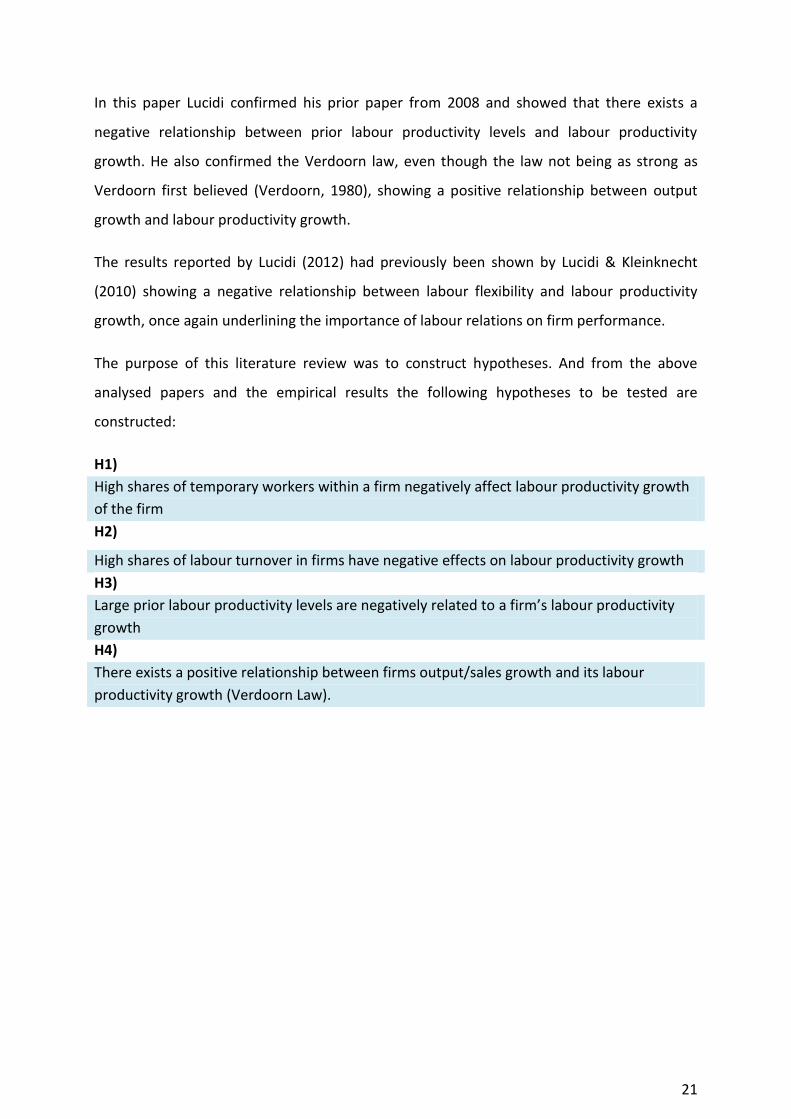
H1)

High shares of temporary workers within a firm negatively affect labour productivity growth

of the firm

H2)

High shares of labour turnover in firms have negative effects on labour productivity growth

H3)

Large prior labour productivity levels are negatively related to a firm’s labour productivity

growth

H4)

There exists a positive relationship between firms output/sales growth and its labour

productivity growth (Verdoorn Law).

22

2.1.2. Innovation regimes and possible effects on labour productivity

It is hard to generalize over a whole economy that labour flexibility hampers labour

productivity within firms. The vast diversity of firms, the industry they are in, the structural

composition (size, age etc.) make it impossible to do such a generalization. Thus researchers

have been investigating what effects flexible labour has on firms under different conditions.

Lucidi & Kleinknecht (2010) and Dekker & Kleinknecht (2011) included firm size and firm age

to see whether different results would emerge. What they did also was including industry

dummies, and showed their results for certain industries so changes between them could be

observed.

There are however theories implying that depending on the firms innovation regime the

effects from flexible labour can have different outcomes. Martínez-Sánchez, et al. (2011)

investigated the effects of human resource practices on innovativeness within firms in the

automotive supplier industry. With empirical analysis they concluded that flexible labour

(specifically temporary labour) negatively affected the innovativeness of the firms whereas

internally flexible labour had positive effects on the innovativeness of the firms.

Kleinknecht, et al. (2006) concluded from their empirical findings that innovative firms

benefit more from reallocation of personnel within the firm (internal labour flexibility). This

suggests that a firms’ innovation regime does have effects on the relationship between

labour flexibility and labour productivity growth.

Acharya et al. (2010) investigated the effects of the legal framework of labour laws and its

possible effects on firms’ innovation. They used data about patents issued in the U.S. by the

United States Patent and Trademark Office. They did a regression analysis where they used

number of patents as the dependent variable and dismissal laws (measured in stringency of

the laws), creditor rights index, import/export and other control variables. The results

revealed that increased stringent dismissal laws positively affect the number of patents

filed/issued supporting the hypothesis that regulated labour markets support innovation

amongst firms.

Like in paragraph 2.1.1 the Italian economy has been the source of investigation when it

comes to labour laws, innovation and productivity. Pieroni & Pompei (2008) conducted a

research in Italian industry by examining the linkage between labour market flexibility and

23

innovation by focusing on different innovation regimes and geographical areas within Italy.

By dividing the industry into high-tech (Schumpeter Mark II) and low-tech (Schumpeter Mark

I) groups they investigated if observable changes in the relationship between innovation and

labour market flexibilities would emerge. They used patents per capita as a dependent

variable to be able to describe the innovation activities within certain regional sectors of

industry. To construct the labour flexibility variable they used the gross job turnover rate

(the sum of job creation and job destruction). They also included wage (blue-collar and

white-collar separately) levels as explanatory variable and year dummies to account for

cyclical fluctuations. Finally to distinguish between low-tech and high-tech industries they

used 10 different industries classified according to OECD classification.

Before dividing into low/high-tech industries, by using a two-way static panel data approach

they concluded that blue collar wages had impact on patent performance, while white collar

wages showed less impact. Interestingly, job turnover showed a non-significant impact on

the patent performance as they expected to begin with. Even after dividing the industries

into low-tech and high-tech groups the job turnover still did not show statistical significance.

They concluded in their models that blue and white collar wage levels exhibited a positive

and significant impact on patent activities while the job turnover showed no statistical

significance in any of their models: However, by interacting the job turnover variable with

geographical areas an observed significance in two of four regions was detected.

Michie & Sheehan (2003) studied the impact of a firm’s use of multiple sorts of flexible

labour, human resource techniques and industrial relation systems on innovation practices.

By conducting a survey they managed to capture data from 361 respondents regarding their

firms’ labour flexibility (internal, external) and human resource practices. The dependent

variable in their model was whether firms innovate or not (also split into process innovation

and product innovation). Their independent variables were age, size, industry dummies and

the flexibility variables including internal flexibility and external flexibility (% of part-time

workers, % of temporary contracts and % of fixed-term, casual or seasonal contracts).

In their estimations the size variables are weak or non-significant for the middle groups

while the largest and smallest firms show significant negative and positive relationship with

the dependent variable. Their estimations also indicate that low road practices, i.e. use of

24

short term contracts, are negatively correlated with innovation, and in contrast the high

road practices, internal flexibility, are positively correlated with innovation. However, only

the internal flexibility and the labour turnover variables were significant while the others

(part-time, temporary and seasonal contracts) did show weak or non-significance in the

relationship with the dependent variable and thus the relationship is less clear.

In their earlier paper, Michie & Sheehan (2001) work with the same data they used in their

paper “Labour marked deregulation, ‘flexibility’ and innovation” from 2003 and come to the

same conclusion as in the 2003 paper. What they test here also is what happens if the

dependent variable is financial performance of the firms, not innovation, and in that sce-

nario both the external and internal flexibility variables positively affect financial perfor-

mance. That could be because using temporary labour forces can, in the short run, decrease

the wage bill of the firms’ (Kleinknecht, et al., 2006) while the internal flexibility can increase

the productivity of the firms in the long run.

Further researches have been done in the field of innovation and labour flexibility. Altuzarra

& Serrano (2010) concluded that a firm’s probability of carrying out R&D activities and

innovation increased up to a certain threshold with increased number of temporary workers.

However, they concluded that this would change after a certain limit.

As mentioned in chapter 1 the different innovation regimes are categorized by Schumpeter

Mark I and Mark II, where the Mark I theory suggested that the industry is characterized by

low entry barriers and high competition, often called ‘garage businesses’ where innovation is

performed in volatile and low concentrated markets. Whereas Mark II suggested that the

industry is made up by large established firms with monopoly power due to large entry

barriers. These industries are often highly concentrated.

From the empirical analyses conducted to research different relationships between labour

flexibility and labour productivity growth under different innovation regimes the following

hypotheses to be tested are laid out:

25

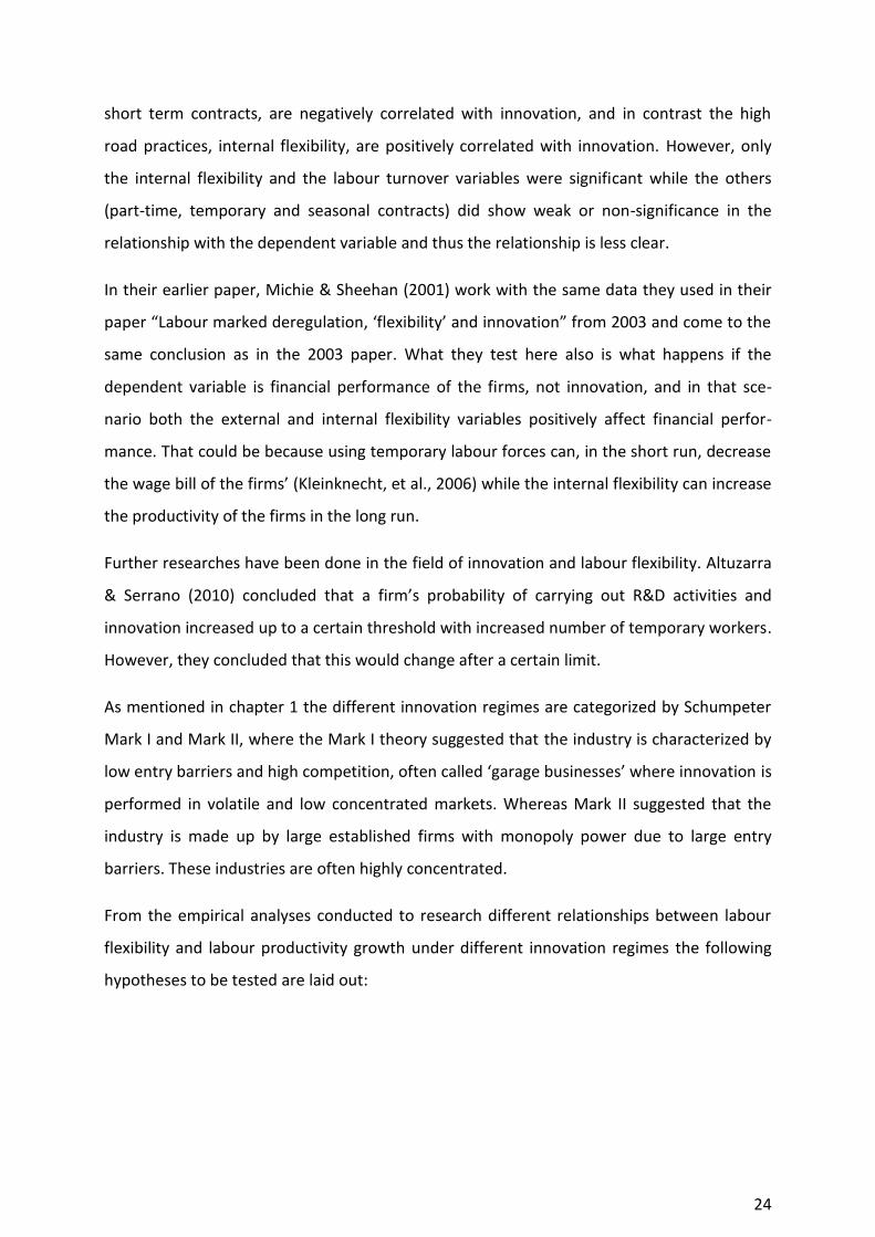
H5)

External flexibility in firms under Schumpeter Mark I innovation regime will have a positive

effect on labour productivity growth

H6)

External flexibility in firms under Schumpeter Mark II innovation regime will have a negative

effect on labour productivity growth

H7)

Internal flexibility in firms under Schumpeter Mark I innovation regime will have a negative

effect on labour productivity growth

H8)

Internal flexibility in firms under Schumpeter Mark II innovation regime will have a positive

effect on labour productivity growth

In the papers reviewed, firm size played a role also and as mentioned before different size

can have different impact when assessing the effects of labour flexibility on firms labour

productivity growth. Thus from the literature review, the following hypothesis is also laid out

to be further investigated:

H9)

Smaller firms will have lower labour productivity growth

The hypotheses laid out in this paragraph 2.1.1 and 2.1.2 will serve as a guideline when

constructing the conceptual model in paragraph 2.2 and will then be evaluated and tested in

chapter 4.

26

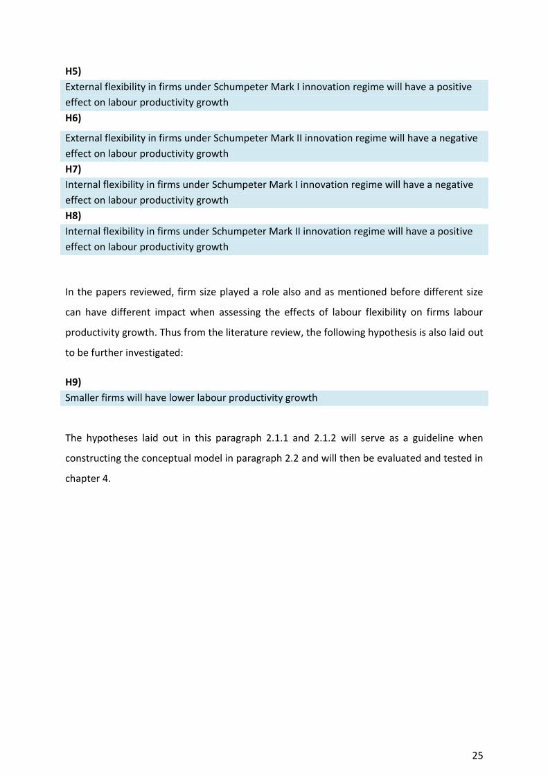
2.2. Conceptual model

On the grounds of the literature review and hypotheses stated above the conceptual model

will be constructed and visualized. As is evident from the literature review there is expected

to be a relationship between flexible labour and labour productivity growth, but as

mentioned in paragraph 2.1.2 an interfering variable in the form of firm’s’ innovation regime

is expected to influence the relationship. Furthermore prior labour productivity levels are

expected to have a negative relationship with the labour productivity growth variable

(Lucidi, 2008) and the output/sales growth of the firm is expected to affect productivity

growth positively (Katz, 1968). Finally, a connection between productivity, industry sectors

(Bester, et al., 2012) and firm size is believed to occur. From this the following visualization

of the model can be seen:

As figure 1 shows we expect a direct relationship between firm size, industry group, sales

growth and labour productivity levels and the dependent variable labour productivity

growth. The relationship between the labour flexibility variables (internal and external) is

expected to be interfered by the Mark I and Mark II innovation regime variables.

- Firm size (+) - Industry group (+/-) - Level of labour productivity (+) - Sales growth (+)

- Internal flexibility (+) - External flexibility (-)

Labour productivity growth

- Mark I - Mark II

Figure 1: The conceptual model

27

3. Research design and methodology

In this chapter the problem will be operationalized and the research design explicitly

explained, followed by a description of the population under study. The chapter ends with

an operational definition of the variables that will be used in the models to be estimated.

3.1. Research design

As is evident from the literature review chapter, many researchers found a negative

relationship between external labour flexibility and labour productivity growth (Lucidi &

Kleinknecht, 2010) (Ortega & Marchante, 2010) and others. The declining labour productivity

growth in Europe during the last decades (Gomez-Salvador, et al., 2006) can have a

significant impact on the competitive level of European countries in the global market. To

further understand the problem the relationship between labour flexibility (external and

internal) and labour productivity growth has to be examined.

There are several ways to examine relationships between variables and one of them is by a

quantitative analysis and that is what will be done in this research. In this paragraph the

design of the research will be discussed and justified from the viewpoint of the problem

statement and prior research carried out concerning labour productivity.

To examine the relationships explained in the conceptual-model in chapter 2 a multiple OLS

regression analysis will be performed by using the statistical program SPSS. By using a

multiple OLS regression, the relationship between multiple independent variables and a

dependent variable can be explained (Cameron & Trivedi, 2005), that is the behavior in the

dependent variable can be explained by the multiple independent variables. Further

explanation of the regression analysis to be performed is explained in detail in paragraph

4.2.

28

3.2. Data collection

In this paragraph the data collection, variables used and the population under study will be

explained in detail.

As mentioned in paragraph 1.7 the data used in this research are extracted from the OSA

database and cover around 3000 Dutch organizations in the entire country. The database

contains more than 500 different questions that the participating firms answer covering a

variety of different factors. In this research only a fraction of the questions is to be used.

Some are used directly and others will be used to construct a final variable that then again is

used in the analysis itself.

The data are time series (panel data) and the timespan used in this research covers the data

published in the years 2004-2010. These will then be pooled together to be used in the OLS

analysis. To construct the sales growth and labour productivity growth variable, information

in the dataset from the last survey is needed. The data for the financial information and fte's

are not available for the years before, that is in the data from 2003 there are only financial

and fte’s information for that particular year (year t) not year t-2. So to tackle that a Python

program was written that compared the company’s ID numbers between two datasets (2003

compared to 2005, 2005 compared to 2007 and so on) and the companies that did not

participate in two consecutive years were thus omitted, and by doing so construction of the

sales growth and labour productivity growth variable was achieved.

To decide what questions answered by the firms’ should be used, the literature review and

conceptual model designed in chapter 2 are used as a roadmap. Here below the hypotheses

stated in chapter 2 will be laid out again and the variables needed to test them will be

assigned to them, the exact construction and operationalization of the variables will be

explained in paragraph 3.3.

Hypothesis 1: to be able to test hypothesis 1 information regarding firms’ use of temporary

work force is needed. Fortunately the OSA database contains information regarding the

percentage of employees on temporary contracts and that data will be used to serve as the

amount of temporary contracts within a firm. The variable labour productivity growth will be

constructed using several other variables, the construction and variables used to construct

29

the labour productivity and the labour productivity growth will be explained in detail in

chapter 3.3.

Hypothesis 2: To test this hypothesis information regarding the total number of employees

within the firms as well as the amount of personnel leaving and entering the firm is needed.

These data are available in the OSA database, that is, total number of personnel, percentage

of personnel leaving and percentage of personnel entering the firm.

Hypothesis 3: To test the validity of this hypothesis there are several variables needed that

together form the prior labour productivity levels. What is needed are the number of Fte’s

(full time equivalents) working for the firms, the total revenue from the firms’ balance sheet

as well as the percentage of sales spent on purchases of intermediate inputs. This

information is available in the OSA database and will be extracted from it to form the

variable itself.

Hypothesis 4: To test the validity of this hypothesis, information to construct the sales

growth of the firms is needed. So information regarding the firms’ revenues, both present

and past, is needed. All information regarding the firms’ financials is available in the OSA

database.

Hypothesis 5-8: Here, information regarding the firm’s innovation regimes that is whether

they belong to Schumpeter Mark I innovation regime or Schumpeter Mark II regime and also

what industry category they belong to is needed. The information regarding industry

category is available in the OSA database but the information regarding the Mark I or Mark II

regime is not available in the OSA database. The information regarding what innovation

regime the firms’ do belong to will be gathered based on their Herfindahl index.

Hypothesis 9: Information regarding firm size in number of employees is available in the OSA

database and will be extracted from it and used in the research.

The data to be used are in raw form when extracted from the OSA database and have to be

transformed slightly before being used in the OLS analysis. The operationalization of each

variable will be explained in detail in paragraph 3.3. A further examination of the variables,

the descriptive statistics, and any data manipulation will be explained in chapter 4.

30

0

500

1000

1500

2000

2500

3000

Withintermediary

goods

Withoutintermediary

goods

3.3. Operational definition of research variables

The operationalization and other calculations with the data will now be explained in detail so

if desired by others they can replicate the research. Each transformation and computation of

selected variables is visualized in mathematical form in appendix A.

Labour productivity

As described in paragraph 1.7 the OSA data chapter the data-sampling was done every other

year and the time-span used in this research is from 2003-2009. The variable labour

productivity is made up from several other variables that are extracted from the OSA

database. The data to be used to construct the labour productivity variable are the number

of employees/fte's (Full-time equivalent), the revenue generated by the firms and the

percentage of sales spent on acquisition of intermediate inputs. The labour productivity

variable was constructed by subtracting the percentage of sales spent on purchases of

intermediate inputs from the turnover and dividing the results by the number of fte’s. It was

both made for the current year and the year before (using information from year t and t-2),

(see appendix A).

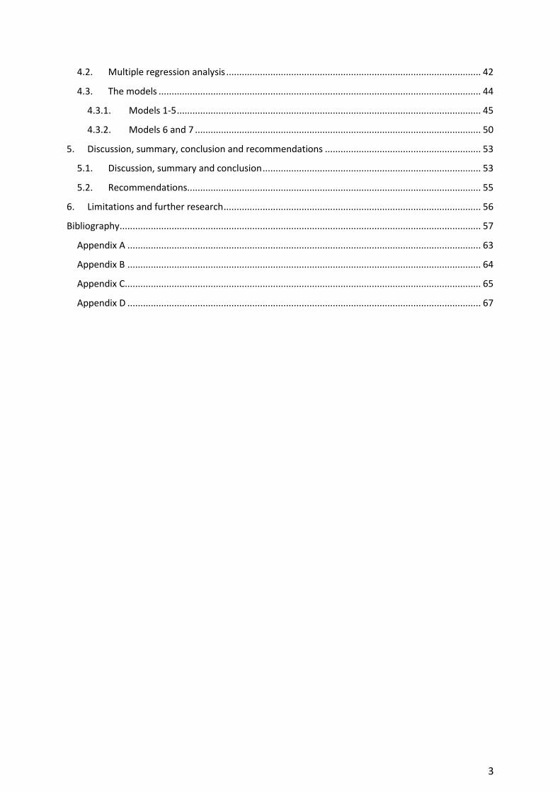
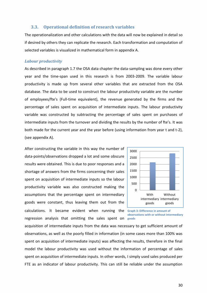
After constructing the variable in this way the number of

data-points/observations dropped a lot and some obscure

results were obtained. This is due to poor responses and a

shortage of answers from the firms concerning their sales

spent on acquisition of intermediate inputs so the labour

productivity variable was also constructed making the

assumptions that the percentage spent on intermediary

goods were constant, thus leaving them out from the

calculations. It became evident when running the

regression analysis that omitting the sales spent on

acquisition of intermediate inputs from the data was necessary to get sufficient amount of

observations, as well as the poorly filled in information (in some cases more than 100% was

spent on acquisition of intermediate inputs) was affecting the results, therefore in the final

model the labour productivity was used without the information of percentage of sales

spent on acquisition of intermediate inputs. In other words, I simply used sales produced per

FTE as an indicator of labour productivity. This can still be reliable under the assumption

Graph 3: Difference in amount of observations with or without intermediary goods

31

that, during the two years’ observation period, the percentage share of intermediary goods

does not change much. To support the reliability of the labour productivity variable after

discarding the % of sales spent on acquisition of intermediate inputs graph 6 in appendix b

compares labour productivity level variables with and without sales spent on acquisition of

intermediate inputs.

Labour productivity growth

To construct the labour productivity growth variable the variables labour productivity from

year t and t-2 were needed. They were then compared to capture the growth in percentages

between the 2 years. When the labour productivity variables contained information on

percentage of sales spent on acquisition of intermediate inputs the labour productivity

growth variable showed many strange data-points (extreme values), and that was one of the

factors in the decision of omitting the percentage of sales spent on acquisition of

intermediate inputs variable in all calculations (see appendix a).

External (numerical) flexibility

The external flexibility was first measured using three variables; i) percentage of personnel

on temporary contracts, ii) personnel turnover (number of personnel leaving and joining the

organization in year t divided by total number of employees) and iii) percentage of

employees from man-power agencies. Later the variable percentage of employees from

man-power agencies was omitted due to the low response rate. At first a model was tested

that incorporated both % of personnel on temporary contracts and also labour turnover, but

due to high correlation between them it was decided to run different models containing the

two variables separately. A correlation table can be seen in appendix b.

Internal (functional) flexibility

To capture the possible impact of the movement of personnel within the firms on labour

productivity growth, the variable was constructed using the percentage of total personnel

reallocated within the company during year t. This information is available in the OSA

database but not many firms responded this question. After combining the surveys about

20% of the firms responded to this question but regardless this variable is one of the main

factors in the analysis and will thus be included to begin with and after testing the models a

decision will be made if it will be used or not in the final model.

32

Sales growth (Verdoorn effect)

According to J.P. Verdoorn who in 1949 examined the relation between output growth and

labour productivity there exist a long run stable relationship between the variables (Katz,

1968). The sales growth (Verdoorn effect) variable was constructed by calculating the annual

growth rate, thus by doing that capture any possible change in output growth of the firms.

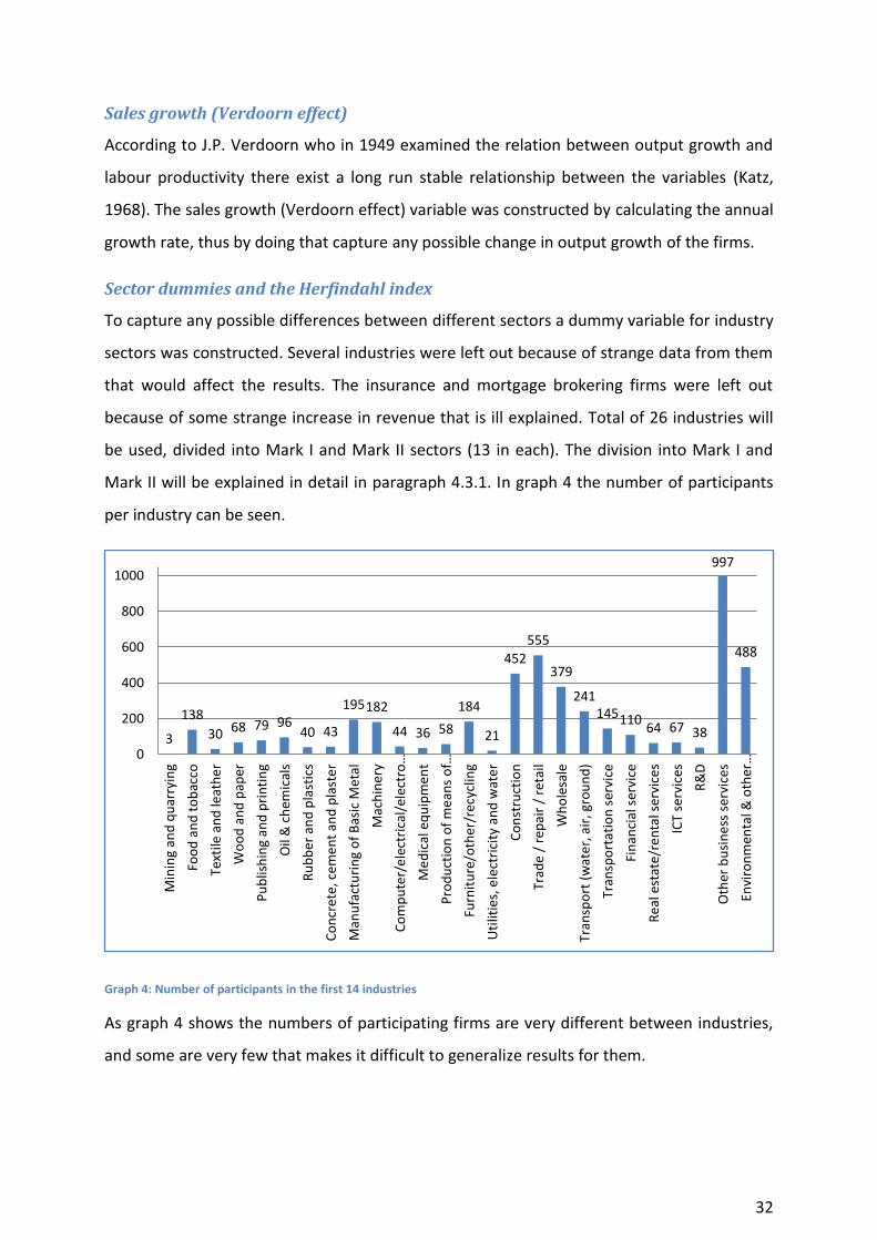
Sector dummies and the Herfindahl index

To capture any possible differences between different sectors a dummy variable for industry

sectors was constructed. Several industries were left out because of strange data from them

that would affect the results. The insurance and mortgage brokering firms were left out

because of some strange increase in revenue that is ill explained. Total of 26 industries will

be used, divided into Mark I and Mark II sectors (13 in each). The division into Mark I and

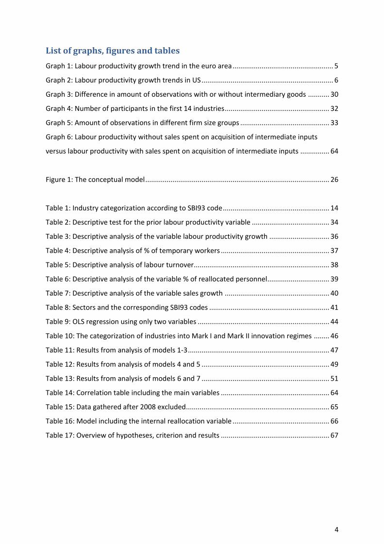
Mark II will be explained in detail in paragraph 4.3.1. In graph 4 the number of participants

per industry can be seen.

Graph 4: Number of participants in the first 14 industries

As graph 4 shows the numbers of participating firms are very different between industries,

and some are very few that makes it difficult to generalize results for them.

3

138

30 68 79 96 40 43

195 182

44 36 58

184

21

452

555

379

241 145 110

64 67 38

997

488

0

200

400

600

800

1000

Min

ing

and

qu

arry

ing

Foo

d a

nd

to

bac

co

Text

ile a

nd

leat

he

r

Wo

od

an

d p

aper

Pu

blis

hin

g an

d p

rin

tin

g

Oil

& c

hem

ical

s

Ru

bb

er a

nd

pla

stic

s

Co

ncr

ete

, ce

me

nt

and

pla

ster

Man

ufa

ctu

rin

g o

f B

asic

Met

al

Mac

hin

ery

Co

mp

ute

r/e

lect

rica

l/el

ectr

o…

Me

dic

al e

qu

ipm

en

t

Pro

du

ctio

n o

f m

ean

s o

f…

Furn

itu

re/o

the

r/re

cycl

ing

Uti

litie

s, e

lect

rici

ty a

nd

wat

er

Co

nst

ruct

ion

Trad

e /

rep

air

/ re

tail

Wh

ole

sale

Tran

spo

rt (

wat

er,

air

, gro

un

d)

Tran

spo

rtat

ion

ser

vice

Fin

anci

al s

ervi

ce

Re

al e

stat

e/r

en

tal s

ervi

ces

ICT

serv

ices

R&

D

Oth

er b

usi

ne

ss s

erv

ices

Envi

ron

men

tal &

oth

er…

33

To see any differences whether companies following Schumpeter Mark I or Schumpeter

Mark II innovation models will have any effect on the labour productivity growth the

industry sectors are assigned a Herfindahl index. The Herfindahl index is a measure of

concentration of R&D in an industry, the value of the index is the sum of the squares of the

R&D shares of all firms in an industry, and higher Herfindahl value is associated with greater

concentration of R&D. The values range from 0-1.

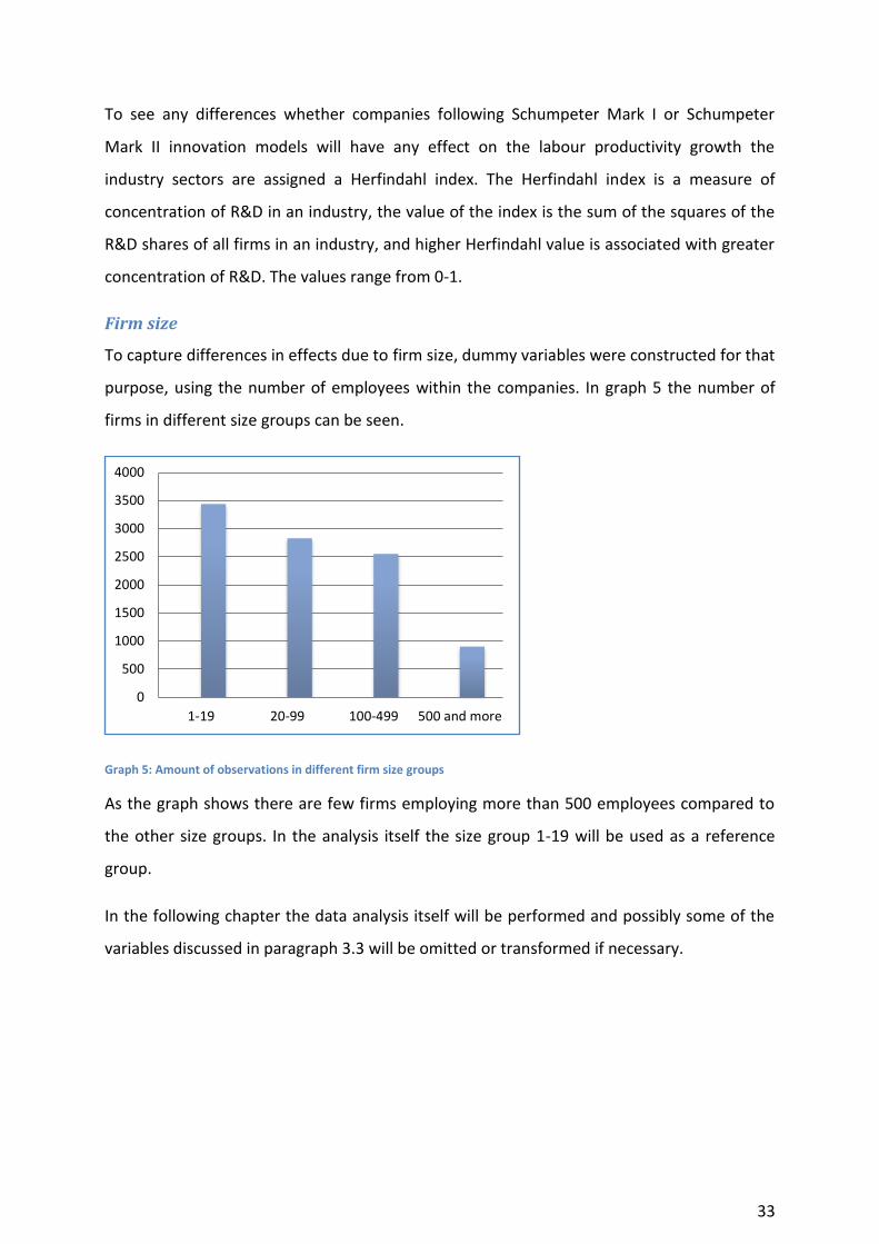
Firm size

To capture differences in effects due to firm size, dummy variables were constructed for that

purpose, using the number of employees within the companies. In graph 5 the number of

firms in different size groups can be seen.

Graph 5: Amount of observations in different firm size groups

As the graph shows there are few firms employing more than 500 employees compared to

the other size groups. In the analysis itself the size group 1-19 will be used as a reference

group.

In the following chapter the data analysis itself will be performed and possibly some of the

variables discussed in paragraph 3.3 will be omitted or transformed if necessary.

0

500

1000

1500

2000

2500

3000

3500

4000

1-19 20-99 100-499 500 and more

34

4. Analysis of data and interpretation of results

In this chapter the procedure of the data analysis will be discussed, descriptive analysis of all

variables will be presented and the cleaning procedure to eliminate outliers (if necessary)

will be explained. Furthermore the regression model will be explained and different analyses

using different models are shown. At the end the results will be elaborated on and

interpreted with respect to the problem definition, research questions and hypotheses.

4.1. Descriptive analysis

In this paragraph the variables to be used in the model will be further examined in detail by

performing descriptive analysis for each variable. After examining each variable further

action will be taken such as cleaning for extreme outliers, by examining the frequency tables,

and performing data transformation if considered necessary.

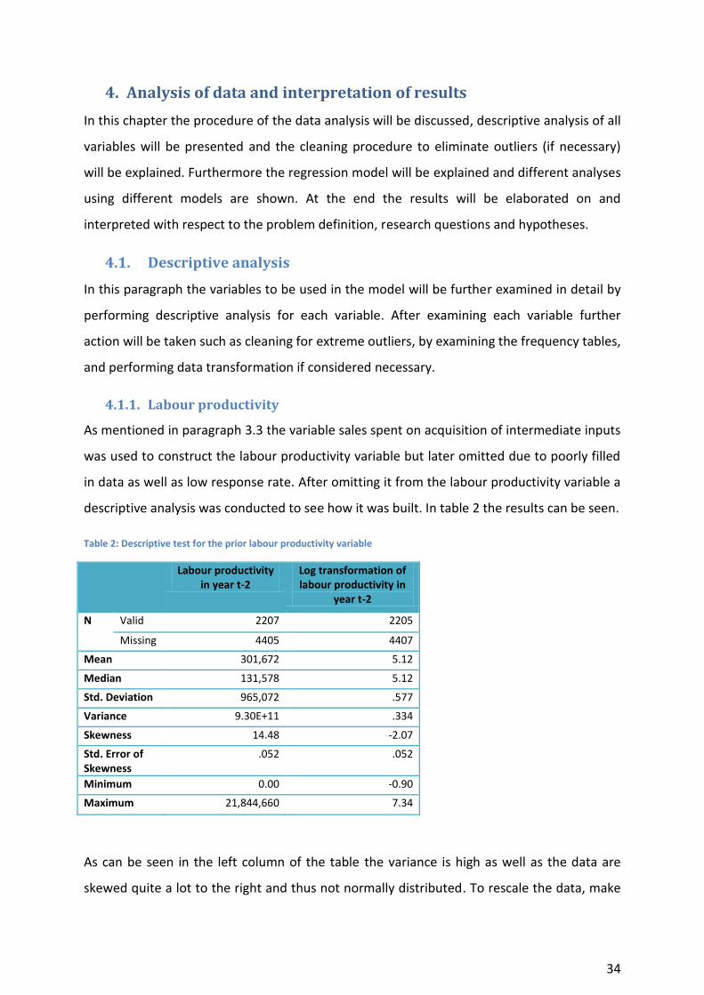
4.1.1. Labour productivity

As mentioned in paragraph 3.3 the variable sales spent on acquisition of intermediate inputs

was used to construct the labour productivity variable but later omitted due to poorly filled

in data as well as low response rate. After omitting it from the labour productivity variable a

descriptive analysis was conducted to see how it was built. In table 2 the results can be seen.

Table 2: Descriptive test for the prior labour productivity variable

Labour productivity in year t-2

Log transformation of labour productivity in

year t-2

N Valid 2207 2205

Missing 4405 4407

Mean 301,672 5.12

Median 131,578 5.12

Std. Deviation 965,072 .577

Variance 9.30E+11 .334

Skewness 14.48 -2.07

Std. Error of Skewness

.052 .052

Minimum 0.00 -0.90

Maximum 21,844,660 7.34

As can be seen in the left column of the table the variance is high as well as the data are

skewed quite a lot to the right and thus not normally distributed. To rescale the data, make

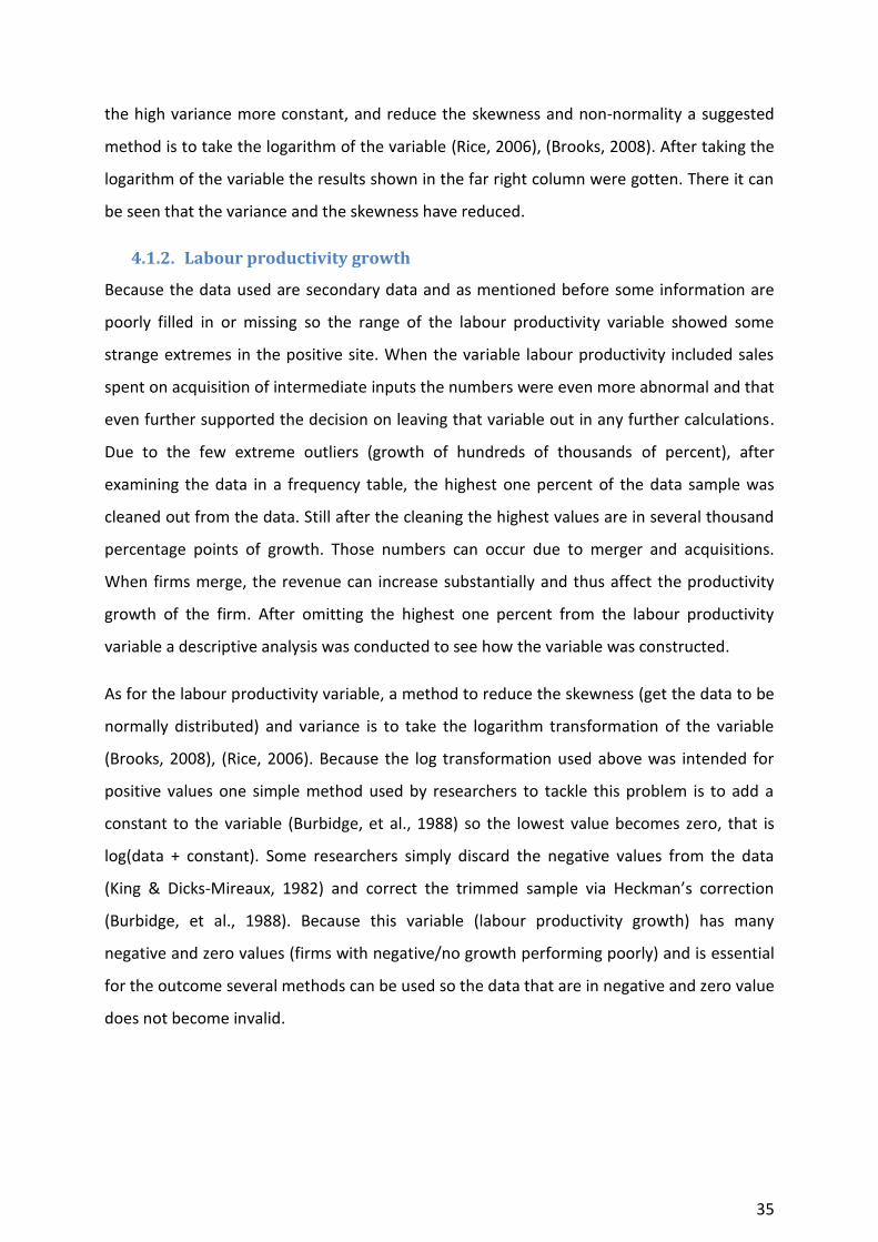
35

the high variance more constant, and reduce the skewness and non-normality a suggested

method is to take the logarithm of the variable (Rice, 2006), (Brooks, 2008). After taking the

logarithm of the variable the results shown in the far right column were gotten. There it can

be seen that the variance and the skewness have reduced.

4.1.2. Labour productivity growth

Because the data used are secondary data and as mentioned before some information are

poorly filled in or missing so the range of the labour productivity variable showed some

strange extremes in the positive site. When the variable labour productivity included sales

spent on acquisition of intermediate inputs the numbers were even more abnormal and that

even further supported the decision on leaving that variable out in any further calculations.

Due to the few extreme outliers (growth of hundreds of thousands of percent), after

examining the data in a frequency table, the highest one percent of the data sample was

cleaned out from the data. Still after the cleaning the highest values are in several thousand

percentage points of growth. Those numbers can occur due to merger and acquisitions.

When firms merge, the revenue can increase substantially and thus affect the productivity

growth of the firm. After omitting the highest one percent from the labour productivity

variable a descriptive analysis was conducted to see how the variable was constructed.

As for the labour productivity variable, a method to reduce the skewness (get the data to be

normally distributed) and variance is to take the logarithm transformation of the variable

(Brooks, 2008), (Rice, 2006). Because the log transformation used above was intended for

positive values one simple method used by researchers to tackle this problem is to add a

constant to the variable (Burbidge, et al., 1988) so the lowest value becomes zero, that is

log(data + constant). Some researchers simply discard the negative values from the data

(King & Dicks-Mireaux, 1982) and correct the trimmed sample via Heckman’s correction

(Burbidge, et al., 1988). Because this variable (labour productivity growth) has many

negative and zero values (firms with negative/no growth performing poorly) and is essential

for the outcome several methods can be used so the data that are in negative and zero value

does not become invalid.

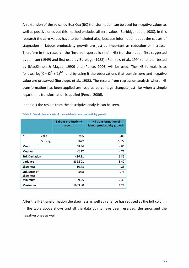
36

An extension of the so called Box-Cox (BC) transformation can be used for negative values as

well as positive ones but this method excludes all zero values (Burbidge, et al., 1988). In this

research the zero values have to be included also, because information about the causes of

stagnation in labour productivity growth are just as important as reduction or increase.

Therefore in this research the ‘inverse hyperbolic sine’ (IHS) transformation first suggested

by Johnson (1949) and first used by Burbidge (1988), (Ramirez, et al., 1994) and later tested

by (MacKinnon & Magee, 1990) and (Pence, 2006) will be used. The IHS formula is as

follows; log(X + (X2 + 1)1/2) and by using it the observations that contain zero and negative

value are preserved (Burbidge, et al., 1988). The results from regression analysis where IHS

transformation has been applied are read as percentage changes, just like when a simple

logarithmic transformation is applied (Pence, 2006).

In table 3 the results from the descriptive analysis can be seen.

Table 3: Descriptive analysis of the variable labour productivity growth

Labour productivity growth.

IHS transformation of labour productivity growth

N Valid 985 985

Missing 5672 5672

Mean 68.84 -.05

Median -2.77 -.77

Std. Deviation 486.31 1.85

Variance 236,501 3.40

Skewness 10.78 .25

Std. Error of Skewness

.078 .078

Minimum -99.95 -2.30

Maximum 8663.90 4.24

After the IHS transformation the skewness as well as variance has reduced as the left column

in the table above shows and all the data points have been reserved, the zeros and the

negative ones as well.

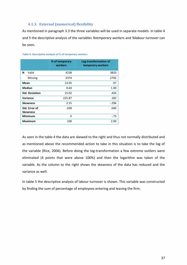
37

4.1.3. External (numerical) flexibility

As mentioned in paragraph 3.3 the three variables will be used in separate models. In table 4

and 5 the descriptive analysis of the variables %temporary workers and %labour turnover can

be seen.

Table 4: Descriptive analysis of % of temporary workers

% of temporary workers

Log transformation of temporary workers

N Valid 4238 3820

Missing 2374 2792

Mean 13.05 .97

Median 8.60 1.00

Std. Deviation 15.02 .426

Variance 225.87 .182

Skewness 2.55 -.296

Std. Error of Skewness

.038 .040

Minimum 0 -.73

Maximum 100 2.00

As seen in the table 4 the data are skewed to the right and thus not normally distributed and

as mentioned above the recommended action to take in this situation is to take the log of

the variable (Rice, 2006). Before doing the log-transformation a few extreme outliers were

eliminated (4 points that were above 100%) and then the logarithm was taken of the

variable. As the column to the right shows the skewness of the data has reduced and the

variance as well.

In table 5 the descriptive analysis of labour turnover is shown. This variable was constructed

by finding the sum of percentage of employees entering and leaving the firm.

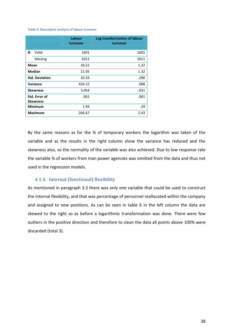
38

Table 5: Descriptive analysis of labour turnover

Labour turnover

Log transformation of labour turnover

N Valid 1601 1601

Missing 5011 5011

Mean 26.52 1.32

Median 21.05 1.32

Std. Deviation 20.59 .296

Variance 424.15 .088

Skewness 3.054 -.031

Std. Error of Skewness

.061 .061

Minimum 1.94 .29

Maximum 266.67 2.43

By the same reasons as for the % of temporary workers the logarithm was taken of the

variable and as the results in the right column show the variance has reduced and the

skewness also, so the normality of the variable was also achieved. Due to low response rate

the variable % of workers from man power agencies was omitted from the data and thus not

used in the regression models.

4.1.4. Internal (functional) flexibility

As mentioned in paragraph 3.3 there was only one variable that could be used to construct

the internal flexibility, and that was percentage of personnel reallocated within the company

and assigned to new positions. As can be seen in table 6 in the left column the data are

skewed to the right so as before a logarithmic transformation was done. There were few

outliers in the positive direction and therefore to clean the data all points above 100% were

discarded (total 3).

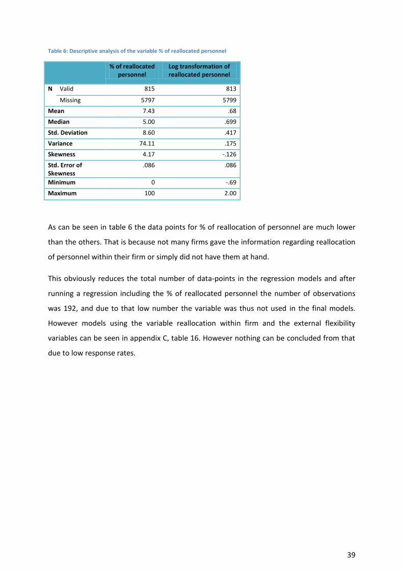
39

Table 6: Descriptive analysis of the variable % of reallocated personnel

% of reallocated personnel

Log transformation of reallocated personnel

N Valid 815 813

Missing 5797 5799

Mean 7.43 .68

Median 5.00 .699

Std. Deviation 8.60 .417

Variance 74.11 .175

Skewness 4.17 -.126

Std. Error of Skewness

.086 .086

Minimum 0 -.69

Maximum 100 2.00

As can be seen in table 6 the data points for % of reallocation of personnel are much lower

than the others. That is because not many firms gave the information regarding reallocation

of personnel within their firm or simply did not have them at hand.

This obviously reduces the total number of data-points in the regression models and after

running a regression including the % of reallocated personnel the number of observations

was 192, and due to that low number the variable was thus not used in the final models.

However models using the variable reallocation within firm and the external flexibility

variables can be seen in appendix C, table 16. However nothing can be concluded from that

due to low response rates.

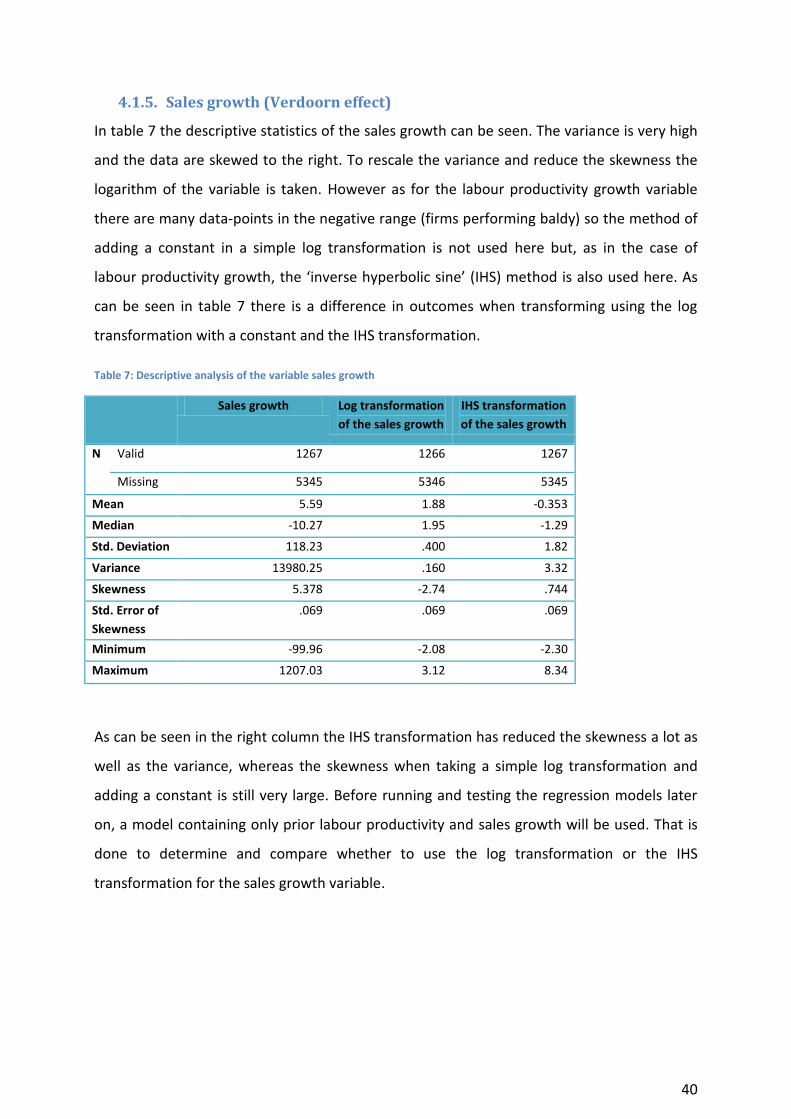
40

4.1.5. Sales growth (Verdoorn effect)

In table 7 the descriptive statistics of the sales growth can be seen. The variance is very high

and the data are skewed to the right. To rescale the variance and reduce the skewness the

logarithm of the variable is taken. However as for the labour productivity growth variable

there are many data-points in the negative range (firms performing baldy) so the method of

adding a constant in a simple log transformation is not used here but, as in the case of

labour productivity growth, the ‘inverse hyperbolic sine’ (IHS) method is also used here. As

can be seen in table 7 there is a difference in outcomes when transforming using the log

transformation with a constant and the IHS transformation.

Table 7: Descriptive analysis of the variable sales growth

Sales growth Log transformation

of the sales growth

IHS transformation

of the sales growth

N Valid 1267 1266 1267

Missing 5345 5346 5345

Mean 5.59 1.88 -0.353

Median -10.27 1.95 -1.29

Std. Deviation 118.23 .400 1.82

Variance 13980.25 .160 3.32

Skewness 5.378 -2.74 .744

Std. Error of

Skewness

.069 .069 .069

Minimum -99.96 -2.08 -2.30

Maximum 1207.03 3.12 8.34

As can be seen in the right column the IHS transformation has reduced the skewness a lot as

well as the variance, whereas the skewness when taking a simple log transformation and

adding a constant is still very large. Before running and testing the regression models later

on, a model containing only prior labour productivity and sales growth will be used. That is

done to determine and compare whether to use the log transformation or the IHS

transformation for the sales growth variable.

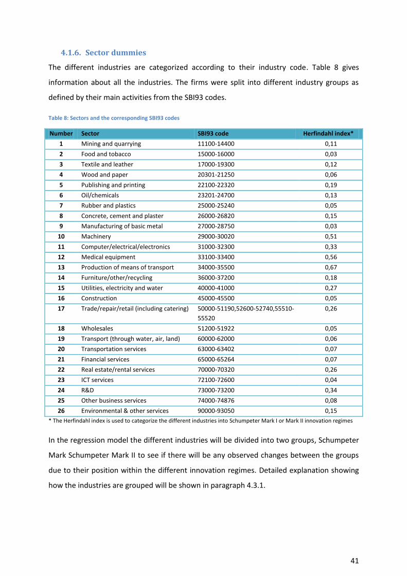
41

4.1.6. Sector dummies

The different industries are categorized according to their industry code. Table 8 gives

information about all the industries. The firms were split into different industry groups as

defined by their main activities from the SBI93 codes.

Table 8: Sectors and the corresponding SBI93 codes

Number Sector SBI93 code Herfindahl index*

1 Mining and quarrying 11100-14400 0,11

2 Food and tobacco 15000-16000 0,03

3 Textile and leather 17000-19300 0,12

4 Wood and paper 20301-21250 0,06

5 Publishing and printing 22100-22320 0,19

6 Oil/chemicals 23201-24700 0,13

7 Rubber and plastics 25000-25240 0,05

8 Concrete, cement and plaster 26000-26820 0,15

9 Manufacturing of basic metal 27000-28750 0,03

10 Machinery 29000-30020 0,51

11 Computer/electrical/electronics 31000-32300 0,33

12 Medical equipment 33100-33400 0,56

13 Production of means of transport 34000-35500 0,67

14 Furniture/other/recycling 36000-37200 0,18

15 Utilities, electricity and water 40000-41000 0,27

16 Construction 45000-45500 0,05

17 Trade/repair/retail (including catering) 50000-51190,52600-52740,55510-

55520

0,26

18 Wholesales 51200-51922 0,05

19 Transport (through water, air, land) 60000-62000 0,06

20 Transportation services 63000-63402 0,07

21 Financial services 65000-65264 0,07

22 Real estate/rental services 70000-70320 0,26

23 ICT services 72100-72600 0,04

24 R&D 73000-73200 0,34

25 Other business services 74000-74876 0,08

26 Environmental & other services 90000-93050 0,15

* The Herfindahl index is used to categorize the different industries into Schumpeter Mark I or Mark II innovation regimes

In the regression model the different industries will be divided into two groups, Schumpeter

Mark Schumpeter Mark II to see if there will be any observed changes between the groups

due to their position within the different innovation regimes. Detailed explanation showing

how the industries are grouped will be shown in paragraph 4.3.1.

42

4.2. Multiple regression analysis

An ordinary least square (OLS) multiple regression analysis will be used to examine the

relationships between the variables of interest. To evaluate relationships between several

independent variables and one or more dependent variable a multiple regression analysis is

one method frequently used. The multiple regression analysis examines the relationship

between the dependent variable (labour productivity growth) and the multiple independent

variables, that is a change in a variable is explained by referencing a change in other

variables (Brooks, 2008). The general model of an ordinary least square regression is:

Where is the dependent variable, is the unknown constant, is the corresponding

unknown coefficient for the independent variable and is the corresponding unknown

coefficient for the independent variable and the corresponding unknown coefficient

for the independent variable k, and finally the random error (Mendenhall, et al., 2008).

The different OLS models to be analysed are explained in further detail in the next chapter.

There are some factors that need to be examined when performing OLS analysis, such as

multicollinearity and, due to nature of the data, autocorrelation (serial-correlation).

Multicollinearity

Multicollinearity occurs when two or more independent variables in a model are highly

correlated with each other. If several independent variables happen to be highly correlated

with each other they can affect the overall outcome of the model and show incorrect results

(York, 2012). The model could look decent and have a large R-square but individual variables

would be insignificant, that is, they would be inflated due to inter-correlation; also the

model becomes highly sensitive to small changes (not robust) (Brooks, 2008). To check for

multicollinearity in the models in chapter 4 the variance inflation factors (VIFs) were

examined. A general rule is that the VIFs should not exceed 10 (Robinson & Schumacker,

2009), in all cases the VIFs were below 2, so no actions needed to be taken regarding

multicollinearity.

43

Autocorrelation (Serial-correlation)

When working with time series data where the data from the different time periods have

been pooled together, the assumption of independence of the errors can be violated

(Bence, 1995) and thus the variables collected in different times become correlated

(autocorrelation), sometimes called serial-correlation. Autocorrelation can affect the

parameter estimates with positive autocorrelation making the parameters looking more

accurate than they actually are and thus the null-hypothesis could be rejected when it

should not be (Williams, 2012).

There is a test for autocorrelation in time-series data like the one used here and that is the

Durbin-Watson test (Brooks, 2008). The Durbin-Watson test examines the relationship

between the error term and its instant preceding value (Durbin & Watson, 1950) in time

series data. The outcome of the Durbin-Watson test is a number in the range from 0-4

(Brooks, 2008) and with a value of 2.0 there is considered to be no autocorrelation, value of

0 is a perfect positive autocorrelation and value of 4 is then a perfect negative

autocorrelation (Durbin & Watson, 1951). When the models that will be described in next

chapter were tested the Durbin-Watson test was also conducted and in all cases it ranged

from 1.9-2.1 and thus no further actions was required regarding autocorrelation in the

models.

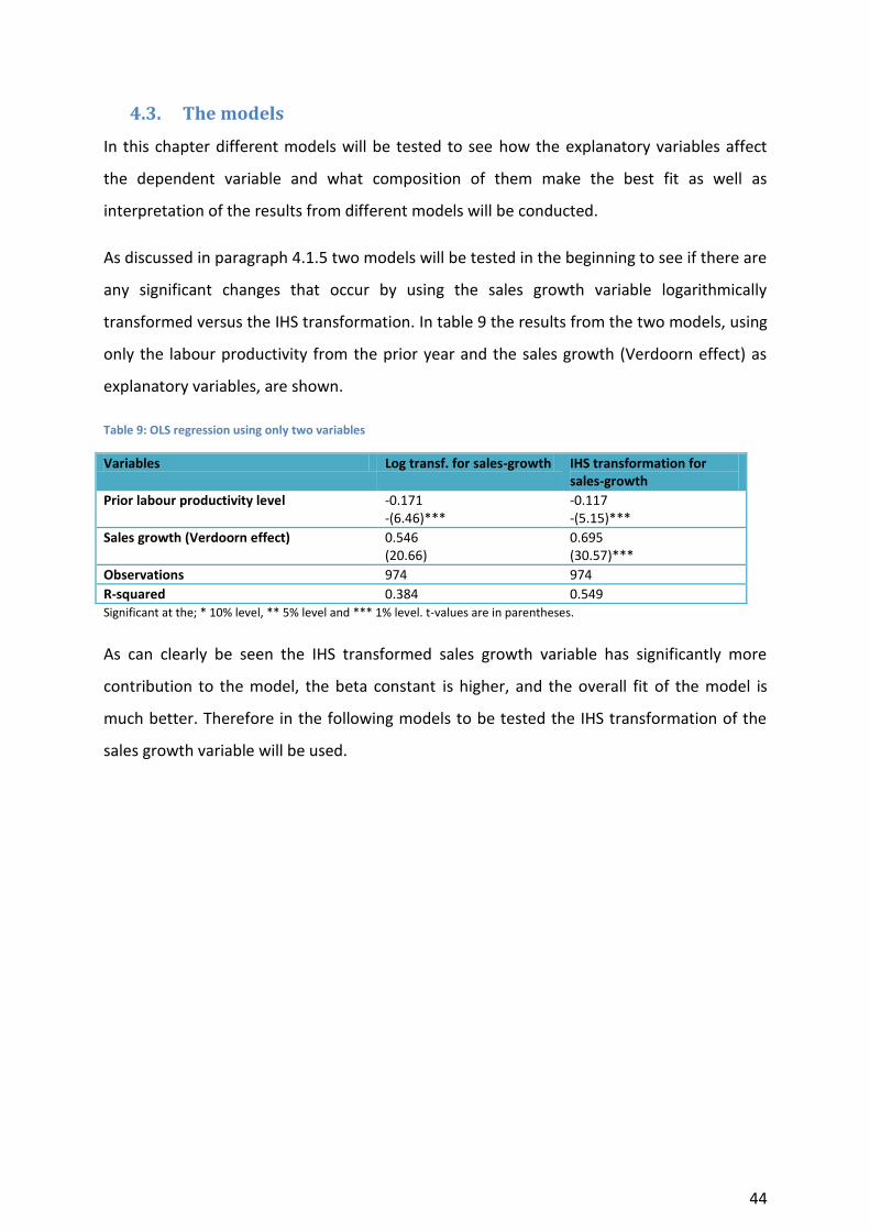
44

4.3. The models

In this chapter different models will be tested to see how the explanatory variables affect

the dependent variable and what composition of them make the best fit as well as

interpretation of the results from different models will be conducted.

As discussed in paragraph 4.1.5 two models will be tested in the beginning to see if there are

any significant changes that occur by using the sales growth variable logarithmically

transformed versus the IHS transformation. In table 9 the results from the two models, using

only the labour productivity from the prior year and the sales growth (Verdoorn effect) as

explanatory variables, are shown.

Table 9: OLS regression using only two variables

Variables Log transf. for sales-growth IHS transformation for sales-growth

Prior labour productivity level -0.171 -(6.46)***

-0.117 -(5.15)***

Sales growth (Verdoorn effect) 0.546 (20.66)

0.695 (30.57)***

Observations 974 974

R-squared 0.384 0.549 Significant at the; * 10% level, ** 5% level and *** 1% level. t-values are in parentheses.

As can clearly be seen the IHS transformed sales growth variable has significantly more

contribution to the model, the beta constant is higher, and the overall fit of the model is

much better. Therefore in the following models to be tested the IHS transformation of the

sales growth variable will be used.

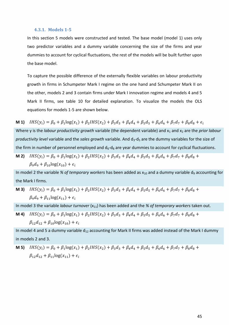
45

4.3.1. Models 1-5

In this section 5 models were constructed and tested. The base model (model 1) uses only

two predictor variables and a dummy variable concerning the size of the firms and year

dummies to account for cyclical fluctuations, the rest of the models will be built further upon

the base model.

To capture the possible difference of the externally flexible variables on labour productivity

growth in firms in Schumpeter Mark I regime on the one hand and Schumpeter Mark II on

the other, models 2 and 3 contain firms under Mark I innovation regime and models 4 and 5

Mark II firms, see table 10 for detailed explanation. To visualize the models the OLS

equations for models 1-5 are shown below.

M 1)

Where y is the labour productivity growth variable (the dependent variable) and x1 and x2 are the prior labour

productivity level variable and the sales growth variable. And d3-d5 are the dummy variables for the size of

the firm in number of personnel employed and d6-d8 are year dummies to account for cyclical fluctuations.

M 2)

In model 2 the variable % of temporary workers has been added as x10 and a dummy variable d9 accounting for

the Mark I firms.

M 3)

In model 3 the variable labour turnover (x11) has been added and the % of temporary workers taken out.

M 4)

In model 4 and 5 a dummy variable d12 accounting for Mark II firms was added instead of the Mark I dummy

in models 2 and 3.

M 5)

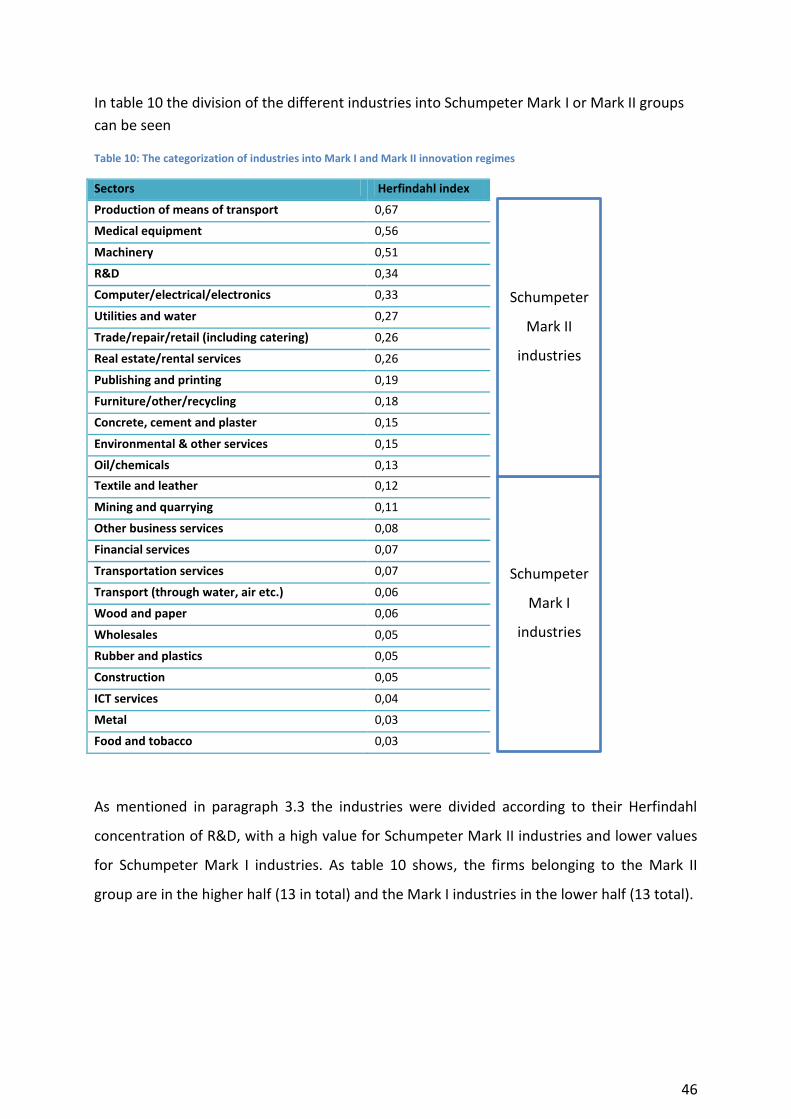
46

In table 10 the division of the different industries into Schumpeter Mark I or Mark II groups

can be seen

Table 10: The categorization of industries into Mark I and Mark II innovation regimes

Sectors Herfindahl index

Production of means of transport 0,67

Medical equipment 0,56

Machinery 0,51

R&D 0,34

Computer/electrical/electronics 0,33

Utilities and water 0,27

Trade/repair/retail (including catering) 0,26

Real estate/rental services 0,26

Publishing and printing 0,19

Furniture/other/recycling 0,18

Concrete, cement and plaster 0,15

Environmental & other services 0,15

Oil/chemicals 0,13

Textile and leather 0,12

Mining and quarrying 0,11

Other business services 0,08

Financial services 0,07

Transportation services 0,07

Transport (through water, air etc.) 0,06

Wood and paper 0,06

Wholesales 0,05

Rubber and plastics 0,05

Construction 0,05

ICT services 0,04

Metal 0,03

Food and tobacco 0,03

As mentioned in paragraph 3.3 the industries were divided according to their Herfindahl

concentration of R&D, with a high value for Schumpeter Mark II industries and lower values

for Schumpeter Mark I industries. As table 10 shows, the firms belonging to the Mark II

group are in the higher half (13 in total) and the Mark I industries in the lower half (13 total).

Schumpeter

Mark I

industries

Schumpeter

Mark II

industries

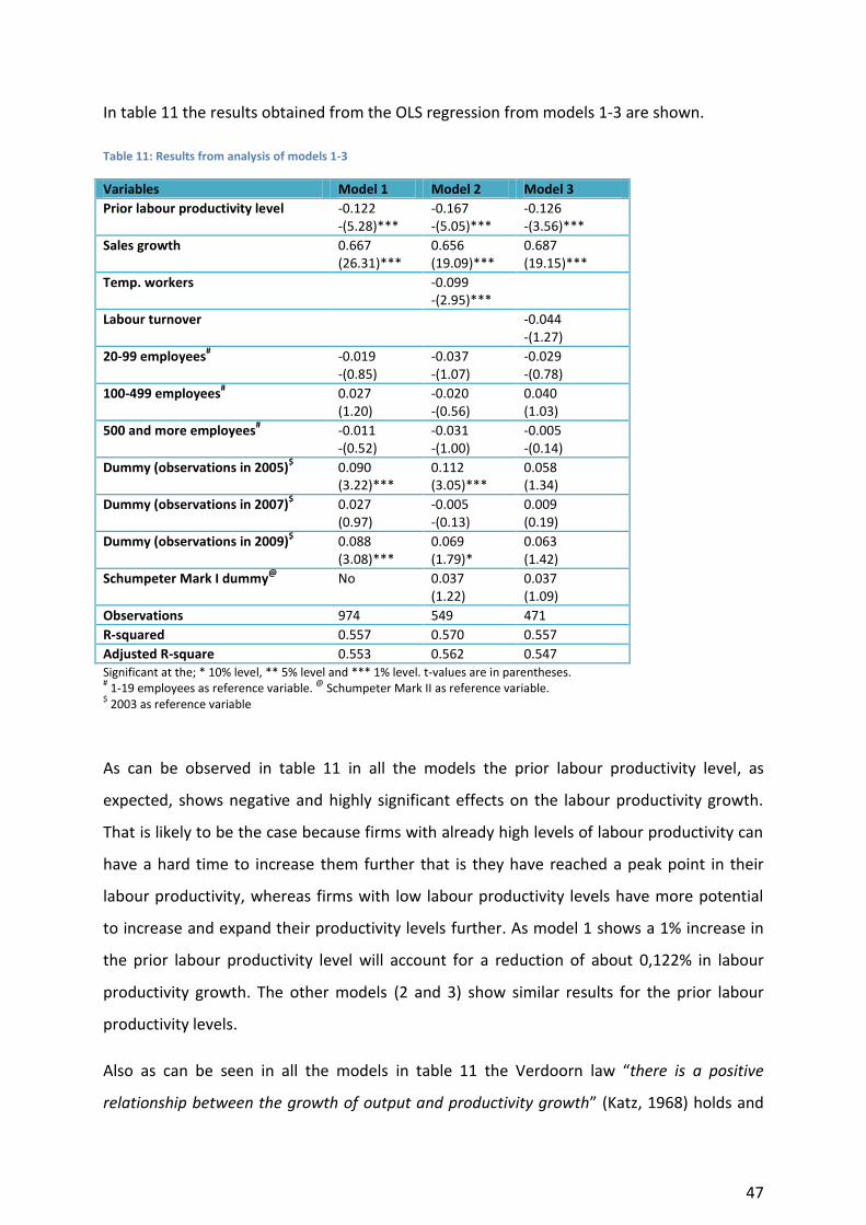
47

In table 11 the results obtained from the OLS regression from models 1-3 are shown.

Table 11: Results from analysis of models 1-3

Variables Model 1 Model 2 Model 3

Prior labour productivity level -0.122 -(5.28)***

-0.167 -(5.05)***

-0.126 -(3.56)***

Sales growth 0.667 (26.31)***

0.656 (19.09)***

0.687 (19.15)***

Temp. workers -0.099 -(2.95)***

Labour turnover

-0.044 -(1.27)

20-99 employees# -0.019

-(0.85) -0.037 -(1.07)

-0.029 -(0.78)

100-499 employees# 0.027

(1.20) -0.020 -(0.56)

0.040 (1.03)

500 and more employees# -0.011

-(0.52) -0.031 -(1.00)

-0.005 -(0.14)

Dummy (observations in 2005)$

0.090 (3.22)***

0.112 (3.05)***

0.058 (1.34)

Dummy (observations in 2007)$

0.027 (0.97)

-0.005 -(0.13)

0.009 (0.19)

Dummy (observations in 2009)$

0.088 (3.08)***

0.069 (1.79)*

0.063 (1.42)

Schumpeter Mark I dummy@

No 0.037 (1.22)

0.037 (1.09)

Observations 974 549 471

R-squared 0.557 0.570 0.557

Adjusted R-square 0.553 0.562 0.547 Significant at the; * 10% level, ** 5% level and *** 1% level. t-values are in parentheses. # 1-19 employees as reference variable.

@ Schumpeter Mark II as reference variable.

$ 2003 as reference variable

As can be observed in table 11 in all the models the prior labour productivity level, as

expected, shows negative and highly significant effects on the labour productivity growth.

That is likely to be the case because firms with already high levels of labour productivity can

have a hard time to increase them further that is they have reached a peak point in their

labour productivity, whereas firms with low labour productivity levels have more potential

to increase and expand their productivity levels further. As model 1 shows a 1% increase in

the prior labour productivity level will account for a reduction of about 0,122% in labour

productivity growth. The other models (2 and 3) show similar results for the prior labour

productivity levels.

Also as can be seen in all the models in table 11 the Verdoorn law “there is a positive

relationship between the growth of output and productivity growth” (Katz, 1968) holds and

48

shows a strong positive and highly significant impact of sales growth on labour productivity

growth. For a 1% increase in sales growth the labour productivity growth increases by

0.667% in model 1, and similar results are observed in the other models, with a slight

increase in model 3, or 0.687% increase in labour productivity growth for a 1% increase in

annual sales growth.

In all the models the firm size variables are not significant and they do change depending on

variables used, but what can be observed is that there is a week negative relationship,

notably for the smallest firm size group and the largest firm size group. The models were

also tested without the firm size variable and that did not affect the other variables in the

models.

According to theories and other empirical results analysed in chapter 2 the percentages of

temporary employees in firms can affect labour productivity growth in a negative way.

Model 2 shows that when the variable % of temporary employees has been added it clearly

shows a negative and significant impact on labour productivity growth. That is a doubling in

the amount of temporary workers used will cause a reduction of 9.9% in labour productivity

growth for Mark I firms. The labour turnover shows also a negative relationship (weakly

significant), with a reduction of 4.4% in labour productivity growth, for Mark I firms, if labour

turnover is doubled.

This result obtained in models 2 and 3 supports hypothesis 1 that high shares of temporary

workers have a negative impact on labour productivity growth in firms. Hypothesis 2 (High

shares of labour turnover in firms have negative effects on the labour productivity growth) is

rejected due to the relatively small t-value though indicating a negative direction.

What can be seen in model 3 is the small reduction in R-square and adjusted R-square when

introducing the labour turnover variable, if this reduction will increase in further models this

loss of efficiency can indicate that the variable might not be relevant for this model (Fomby,

1981) (Granger & Newbold , 1974) and does not add any information to the model. If the

reduction will however be as little as observed it will still be used in the next models.

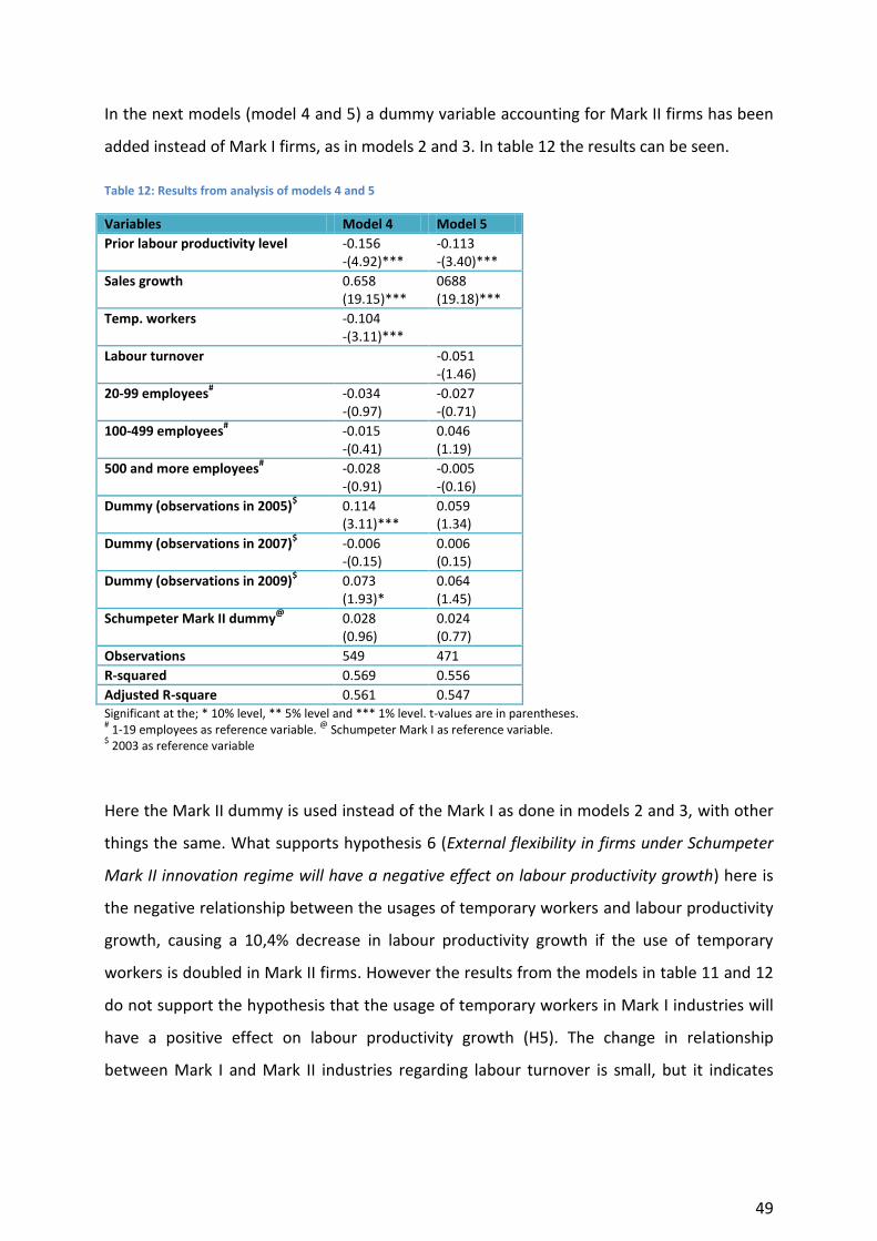
49

In the next models (model 4 and 5) a dummy variable accounting for Mark II firms has been

added instead of Mark I firms, as in models 2 and 3. In table 12 the results can be seen.

Table 12: Results from analysis of models 4 and 5

Variables Model 4 Model 5

Prior labour productivity level -0.156 -(4.92)***

-0.113 -(3.40)***

Sales growth 0.658 (19.15)***

0688 (19.18)***

Temp. workers -0.104 -(3.11)***

Labour turnover -0.051 -(1.46)

20-99 employees# -0.034

-(0.97) -0.027 -(0.71)

100-499 employees# -0.015

-(0.41) 0.046 (1.19)

500 and more employees# -0.028

-(0.91) -0.005 -(0.16)

Dummy (observations in 2005)$ 0.114

(3.11)*** 0.059 (1.34)

Dummy (observations in 2007)$ -0.006

-(0.15) 0.006 (0.15)

Dummy (observations in 2009)$ 0.073

(1.93)* 0.064 (1.45)

Schumpeter Mark II dummy@

0.028 (0.96)

0.024 (0.77)

Observations 549 471

R-squared 0.569 0.556

Adjusted R-square 0.561 0.547 Significant at the; * 10% level, ** 5% level and *** 1% level. t-values are in parentheses. # 1-19 employees as reference variable.

@ Schumpeter Mark I as reference variable.

$ 2003 as reference variable

Here the Mark II dummy is used instead of the Mark I as done in models 2 and 3, with other

things the same. What supports hypothesis 6 (External flexibility in firms under Schumpeter

Mark II innovation regime will have a negative effect on labour productivity growth) here is

the negative relationship between the usages of temporary workers and labour productivity

growth, causing a 10,4% decrease in labour productivity growth if the use of temporary

workers is doubled in Mark II firms. However the results from the models in table 11 and 12

do not support the hypothesis that the usage of temporary workers in Mark I industries will

have a positive effect on labour productivity growth (H5). The change in relationship

between Mark I and Mark II industries regarding labour turnover is small, but it indicates

50

(though weakly significant) however that high labour turnover hampers labour productivity

growth in firms regardless of their innovation regime.

For the firm size variables the same can be observed in models 4 and 5: firm size is insigni-

ficant and thus it indicates that they do not matter for labour productivity growth. All the

models were also tested without the size variables to see if it affected the other variables,

and it did not pose any changes to the remainder of the variables. Because of the strong

positive relationship between firm size and labour productivity, obtained by Dekker and

Kleinknecht (2011) when they researched data from Dutch industries, it was decided to run

the model again discarding the data gathered after the 2008 financial crisis, because the

distortion on the market following the crisis might have impacted the market. But discarding

data after 2008 did not change the firm size variable, the results can be seen in appendix c.

What can also be seen in the models is that year 2005 and 2009 are significant and thus do

not show same characters like the reference variable (year 2003). The 2007 variable is

insignificant and is therefore similar in behavior as the reference variable, thus indicating

cyclical fluctuation in the business cycles.

4.3.2. Models 6 and 7

As previously discussed the theory suggests that firms under Schumpeter Mark I innovation

regime will perform better in externally flexible markets (that is high share of temporary

workers etc.) than Schumpeter Mark II firms (Zhou, et al., 2011). To check whether the data

used in this research will give similar conclusion two new models were constructed (model 6

and 7) and an interaction term was added to the model. In the models the Mark II dummy

was multiplied with the % of temporary worker variable and the labour turnover variable. On

next page the regression equation for models 6 and 7 can be seen.

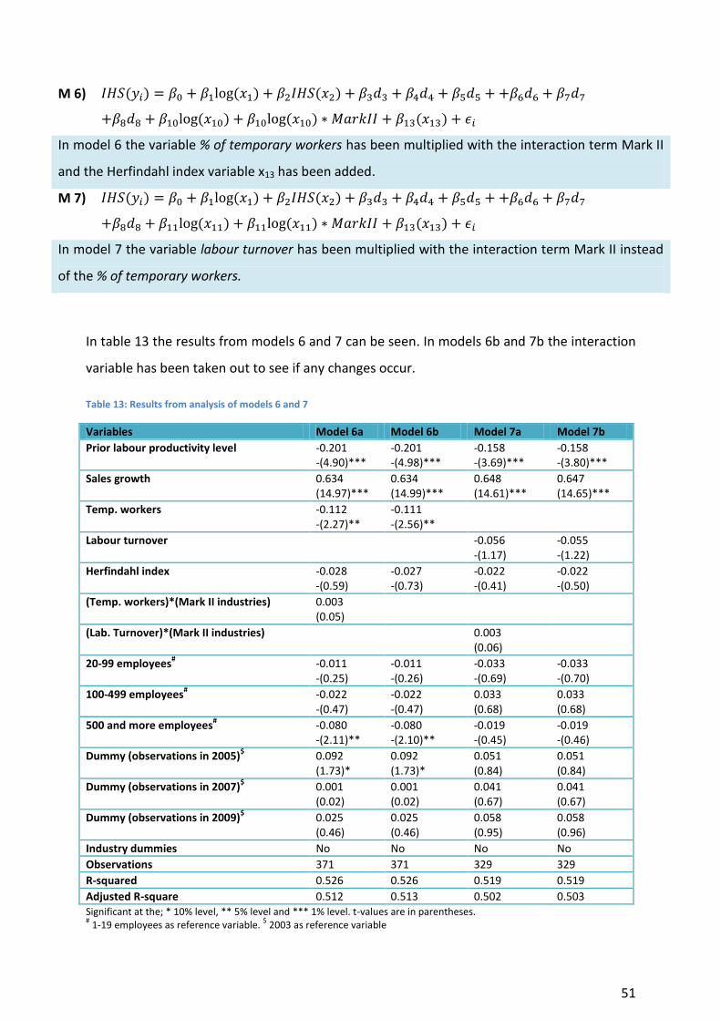
51

M 6)

In model 6 the variable % of temporary workers has been multiplied with the interaction term Mark II

and the Herfindahl index variable x13 has been added.

M 7)

In model 7 the variable labour turnover has been multiplied with the interaction term Mark II instead

of the % of temporary workers.

In table 13 the results from models 6 and 7 can be seen. In models 6b and 7b the interaction

variable has been taken out to see if any changes occur.

Table 13: Results from analysis of models 6 and 7

Variables Model 6a Model 6b Model 7a Model 7b

Prior labour productivity level -0.201 -(4.90)***

-0.201 -(4.98)***

-0.158 -(3.69)***

-0.158 -(3.80)***

Sales growth 0.634 (14.97)***

0.634 (14.99)***

0.648 (14.61)***

0.647 (14.65)***

Temp. workers -0.112 -(2.27)**

-0.111 -(2.56)**

Labour turnover -0.056 -(1.17)

-0.055 -(1.22)

Herfindahl index -0.028 -(0.59)

-0.027 -(0.73)

-0.022 -(0.41)

-0.022 -(0.50)

(Temp. workers)*(Mark II industries) 0.003 (0.05)

(Lab. Turnover)*(Mark II industries) 0.003 (0.06)

20-99 employees# -0.011

-(0.25) -0.011 -(0.26)

-0.033 -(0.69)

-0.033 -(0.70)

100-499 employees# -0.022

-(0.47) -0.022 -(0.47)

0.033 (0.68)

0.033 (0.68)

500 and more employees# -0.080

-(2.11)** -0.080 -(2.10)**

-0.019 -(0.45)

-0.019 -(0.46)

Dummy (observations in 2005)$ 0.092

(1.73)* 0.092 (1.73)*

0.051 (0.84)

0.051 (0.84)

Dummy (observations in 2007)$ 0.001

(0.02) 0.001 (0.02)

0.041 (0.67)

0.041 (0.67)

Dummy (observations in 2009)$ 0.025

(0.46) 0.025 (0.46)

0.058 (0.95)

0.058 (0.96)

Industry dummies No No No No

Observations 371 371 329 329

R-squared 0.526 0.526 0.519 0.519

Adjusted R-square 0.512 0.513 0.502 0.503 Significant at the; * 10% level, ** 5% level and *** 1% level. t-values are in parentheses. # 1-19 employees as reference variable.

$ 2003 as reference variable

52

In models 6a and 7a it can be observed that the interaction variable, the labour turnover

variable and the Herfindahl variables are all insignificant. The industry dummies are not used

because they correlate highly with the Herfindahl index variable. The prior labour

productivity variable and the sales growth variable behave like they did in the previous

models, further supporting the hypotheses (H3 and H4) laid out in chapter 2. What can be

observed in models 6b and 7b is that no changes occur (in t-value, constants or r-square)

after eliminating the interaction variable, indicating it did not bring value to the models.

53

5. Discussion, summary, conclusion and recommendations

5.1. Discussion, summary and conclusion

In this research we have investigated the relationship between various independent

variables and their effects on labour productivity growth in Dutch firms, covering data from

2003-2009. The variables of interest are labour flexibility, firms’ prior labour productivity

levels, the annual sales growth (Verdoorn effect), firm size, and industry dummies. After

putting forward the problem statement and research question a detailed literature review

was conducted by examining previous researches in the field of human resource manage-

ment, labour laws and regulation, labour flexibility, productivity, and sales.

After reviewing the current literature and extracting information about previous empirical

results hypotheses to be tested were constructed. We expected a negative impact to be

exerted on labour productivity growth in firms using externally flexible labour (i.e. temporary

contracts and high labour turnover) and therefore we put forward hypothesis 1 which is

“High shares of temporary workers within a firm negatively affects the labour productivity

growth of the firm”. In appendix d, table 17, an overview of the hypotheses the criterion and

results can be seen.

Hypothesis (6) stating “External flexibility in firms under Schumpeter Mark II innovation

regime will have a negative effect on labour productivity growth” cannot be rejected, in

terms of temporary labour forces, where negative relationships were found. However

hypothesis (5) stating “External flexibility in firms under Schumpeter Mark I innovation

regime will have a positive effect on labour productivity growth” is rejected because the

relationship was negative as well as significant, not positive as believed to be the case in the

beginning.

To capture any possible changes in impacts between firms in different innovation regimes

we tested models involving firms characterized as Schumpeter Mark I and Schumpeter Mark

II firms. What could be observed in both cases is that the usage of temporary labour forces

negatively affects the labour productivity growth in firms, with a slightly higher negative

impact for firms in Schumpeter Mark II regimes.

54

To account for the impact of high labour turnover two separate models including labour

turnover instead of the % of temporary labour forces were constructed. In that case we did

not get significant results, but the direction of the relationship implied a negative impact

from labour turnover on labour productivity growth. From these results we reject hypothesis

2 implying a negative effects from labour turnover on labour productivity growth.

As previous researches suggested by Dekker & Kleinknecht (2011) and Ortega & Marchante

(2010) we were expecting a negative relationship between the prior level of labour

productivity and labour productivity growth. In all our models there was a highly significant

and negative relationship between the variables that supported previous findings and our

hypothesis 3; “Large prior labour productivity levels are negatively related to firms labour

productivity growth levels“. These findings indicate that firms with already high levels of

productivity have little ”space“ to further improve them whereas firms with low levels have

the potential to improve the productivity further.

As expected, Verdoorn’s Law that implies a positive relationship between sales growth and

productivity growth, did hold in our research, as previous findings also indicated. We found a

very strong positive relationship between sales growth and productivity growth, showing

little changes regardless of industry implying that a rise in productivity growth can be related

to an increase of sales growth in all industries.

What was interesting, however, is that the firm size variables did not show any significant

results as expected. Contrary to Dekker and Kleinknecht (2011) that found a positive rela-

tionship between firm size and labour productivity growth, our results implied no such rela-

tionship. We therefore reject our hypothesis 9 (Smaller firms will have lower labour pro-

ductivity growth) because of the non-significant relationship in our estimates.

In our last models (model 6 and 7) we did not get the significance as expected and therefore

cannot conclude on the interaction terms applied to the flexibility variables. However, the

strong impact from prior productivity levels as well as the sales growth are once again

evident and show the importance of them in regard of labour productivity growth.

55

Finally to answer our research question: “What factors do affect firms’ labour productivity

growth in market orientated firms that can be characterized as either Schumpeter Mark I or

Schumpeter Mark II firms?” we can conclude from our models that the usage of temporary

labour forces, the prior productivity levels as well as the annual sales-growth of the firms do

indeed affect labour productivity growth. Answering sub-question one: “How and to what

extent does internal (functional) labour flexibility affect firms’ labour productivity growth?” is

not possible due to low response rates regarding internal reallocation of personnel within

firms. However answering the second sub-question: “How and to what extent does external

(numerical) labour flexibility affect firms’ labour productivity growth?” can be done by

looking at the results in models 1-5. There it can be seen that external flexibility (in terms of

temporary contracts) does negatively affect labour productivity growth. However there

might be, and probably are, other factors as well, not tested here, that can affect labour

productivity growth in firms, but that, on its own, has to be the subject of another research.

5.2. Recommendations

Our aim with this research was to ”investigate the significance of labour flexibility and how

the flexibility affects labour productivity growth in market orientated firm’s following either

Schumpeter Mark I or Mark II innovation models“ and, by doing so, providing a guidance for

human resource managers, lawmakers and others that can, in the power of their position,

influence the labour market.

Our conclusions shed light on several important factors that affect labour productivity

growth in firms, indicating that the usage of externally flexible labour forces in the form of

temporary/short term contracts reduces labour productivity growth. Based on the results

from the analysis it is recommended that care is taken when choosing the composition of

the workforce as well as when constructing and implementing regulations.

56

6. Limitations and further research

This research, as all other, faces limitations in any form whether it is due to imperfect data,

imperfect programs used, or just plain time constraint. The main limitation faced by this

research is the data that are used to test the reliability of the theories. The fact that the data

are gathered by external parties, not the researcher, constrains the execution of the

research. Many firms did not answer questions regarding the internal movement of its

employees and that resulted in non-conclusive results concerning that particular variable.

The imperfect entry of data also poses limitations when extreme outliers are observed.

For the possibility of further research in this area, conducting an own survey to minimize

data loss could be done despite being time consuming. It would, however, be interesting to

do so to strive for increase in the response rate of internal movement of employees whereas

the literature suggests that it could have a significant impact on labour productivity growth.

Though, posed to limitations, this research has contributed to the ever-expanding know-

ledge in labour economics, where this area of study is gradually more being examined and it

will be exciting to follow future researches and their contributions to the literature.

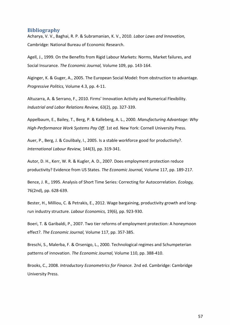
57

Bibliography Acharya, V. V., Baghai, R. P. & Subramanian, K. V., 2010. Labor Laws and Innovation,

Cambridge: National Bureau of Economic Research.

Agell, J., 1999. On the Benefits from Rigid Labour Markets: Norms, Market failures, and

Social Insurance. The Economic Journal, Volume 109, pp. 143-164.

Aiginger, K. & Guger, A., 2005. The European Social Model: from obstruction to advantage.

Progressive Politics, Volume 4.3, pp. 4-11.

Altuzarra, A. & Serrano, F., 2010. Firms' Innovation Activity and Numerical Flexibility.

Industrial and Labor Relations Review, 63(2), pp. 327-339.

Appelbaum, E., Bailey, T., Berg, P. & Kalleberg, A. L., 2000. Manufacturing Advantage: Why

High-Performance Work Systems Pay Off. 1st ed. New York: Cornell University Press.

Auer, P., Berg, J. & Coulibaly, I., 2005. Is a stable workforce good for productivity?.

International Labour Review, 144(3), pp. 319-341.

Autor, D. H., Kerr, W. R. & Kugler, A. D., 2007. Does employment protection reduce

productivity? Evidence from US States. The Economic Journal, Volume 117, pp. 189-217.

Bence, J. R., 1995. Analysis of Short Time Series: Correcting for Autocorrelation. Ecology,

76(2nd), pp. 628-639.

Bester, H., Milliou, C. & Petrakis, E., 2012. Wage bargaining, productivity growth and long-

run industry structure. Labour Economics, 19(6), pp. 923-930.

Boeri, T. & Garibaldi, P., 2007. Two tier reforms of employment protection: A honeymoon

effect?. The Economic Journal, Volume 117, pp. 357-385.

Breschi, S., Malerba, F. & Orsenigo, L., 2000. Technological regimes and Schumpeterian

patterns of innovation. The Economic Journal, Volume 110, pp. 388-410.

Brooks, C., 2008. Introductory Econometrics for Finance. 2nd ed. Cambridge: Cambridge

University Press.

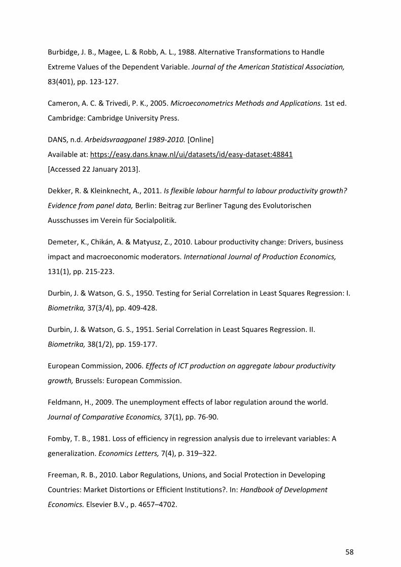
58

Burbidge, J. B., Magee, L. & Robb, A. L., 1988. Alternative Transformations to Handle

Extreme Values of the Dependent Variable. Journal of the American Statistical Association,

83(401), pp. 123-127.

Cameron, A. C. & Trivedi, P. K., 2005. Microeconometrics Methods and Applications. 1st ed.

Cambridge: Cambridge University Press.

DANS, n.d. Arbeidsvraagpanel 1989-2010. [Online]

Available at: https://easy.dans.knaw.nl/ui/datasets/id/easy-dataset:48841

[Accessed 22 January 2013].

Dekker, R. & Kleinknecht, A., 2011. Is flexible labour harmful to labour productivity growth?

Evidence from panel data, Berlin: Beitrag zur Berliner Tagung des Evolutorischen

Ausschusses im Verein für Socialpolitik.

Demeter, K., Chikán, A. & Matyusz, Z., 2010. Labour productivity change: Drivers, business

impact and macroeconomic moderators. International Journal of Production Economics,

131(1), pp. 215-223.

Durbin, J. & Watson, G. S., 1950. Testing for Serial Correlation in Least Squares Regression: I.

Biometrika, 37(3/4), pp. 409-428.

Durbin, J. & Watson, G. S., 1951. Serial Correlation in Least Squares Regression. II.

Biometrika, 38(1/2), pp. 159-177.

European Commission, 2006. Effects of ICT production on aggregate labour productivity

growth, Brussels: European Commission.

Feldmann, H., 2009. The unemployment effects of labor regulation around the world.

Journal of Comparative Economics, 37(1), pp. 76-90.

Fomby, T. B., 1981. Loss of efficiency in regression analysis due to irrelevant variables: A

generalization. Economics Letters, 7(4), p. 319–322.

Freeman, R. B., 2010. Labor Regulations, Unions, and Social Protection in Developing

Countries: Market Distortions or Efficient Institutions?. In: Handbook of Development

Economics. Elsevier B.V., p. 4657–4702.

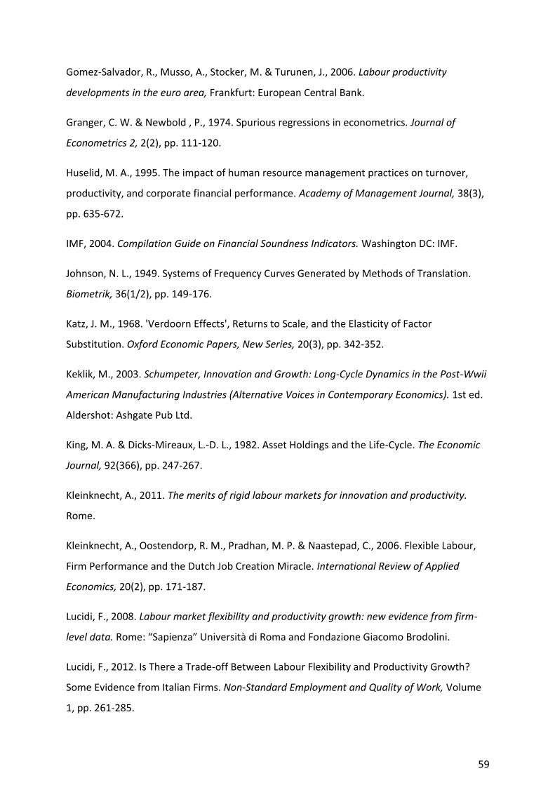
59

Gomez-Salvador, R., Musso, A., Stocker, M. & Turunen, J., 2006. Labour productivity

developments in the euro area, Frankfurt: European Central Bank.

Granger, C. W. & Newbold , P., 1974. Spurious regressions in econometrics. Journal of

Econometrics 2, 2(2), pp. 111-120.

Huselid, M. A., 1995. The impact of human resource management practices on turnover,

productivity, and corporate financial performance. Academy of Management Journal, 38(3),

pp. 635-672.

IMF, 2004. Compilation Guide on Financial Soundness Indicators. Washington DC: IMF.

Johnson, N. L., 1949. Systems of Frequency Curves Generated by Methods of Translation.

Biometrik, 36(1/2), pp. 149-176.

Katz, J. M., 1968. 'Verdoorn Effects', Returns to Scale, and the Elasticity of Factor

Substitution. Oxford Economic Papers, New Series, 20(3), pp. 342-352.

Keklik, M., 2003. Schumpeter, Innovation and Growth: Long-Cycle Dynamics in the Post-Wwii

American Manufacturing Industries (Alternative Voices in Contemporary Economics). 1st ed.

Aldershot: Ashgate Pub Ltd.

King, M. A. & Dicks-Mireaux, L.-D. L., 1982. Asset Holdings and the Life-Cycle. The Economic

Journal, 92(366), pp. 247-267.

Kleinknecht, A., 2011. The merits of rigid labour markets for innovation and productivity.

Rome.

Kleinknecht, A., Oostendorp, R. M., Pradhan, M. P. & Naastepad, C., 2006. Flexible Labour,

Firm Performance and the Dutch Job Creation Miracle. International Review of Applied

Economics, 20(2), pp. 171-187.

Lucidi, F., 2008. Labour market flexibility and productivity growth: new evidence from firm-

level data. Rome: “Sapienza” Università di Roma and Fondazione Giacomo Brodolini.

Lucidi, F., 2012. Is There a Trade-off Between Labour Flexibility and Productivity Growth?

Some Evidence from Italian Firms. Non-Standard Employment and Quality of Work, Volume

1, pp. 261-285.

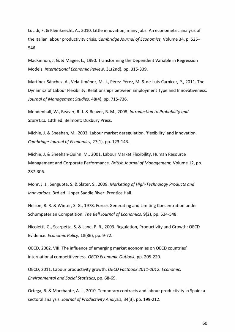
60

Lucidi, F. & Kleinknecht, A., 2010. Little innovation, many jobs: An econometric analysis of

the Italian labour productivity crisis. Cambridge Journal of Economics, Volume 34, p. 525–

546.

MacKinnon, J. G. & Magee, L., 1990. Transforming the Dependent Variable in Regression

Models. International Economic Review, 31(2nd), pp. 315-339.

Martínez-Sánchez, A., Vela-Jiménez, M.-J., Pérez-Pérez, M. & de-Luis-Carnicer, P., 2011. The

Dynamics of Labour Flexibility: Relationships between Employment Type and Innovativeness.

Journal of Management Studies, 48(4), pp. 715-736.

Mendenhall, W., Beaver, R. J. & Beaver, B. M., 2008. Introduction to Probability and

Statistics. 13th ed. Belmont: Duxbury Press.

Michie, J. & Sheehan, M., 2003. Labour market deregulation, 'flexibility' and innovation.

Cambridge Journal of Economics, 27(1), pp. 123-143.

Michie, J. & Sheehan-Quinn, M., 2001. Labour Market Flexibility, Human Resource

Management and Corporate Performance. British Journal of Management, Volume 12, pp.

287-306.

Mohr, J. J., Sengupta, S. & Slater, S., 2009. Marketing of High-Technology Products and

Innovations. 3rd ed. Upper Saddle River: Prentice Hall.

Nelson, R. R. & Winter, S. G., 1978. Forces Generating and Limiting Concentration under

Schumpeterian Competition. The Bell Journal of Economics, 9(2), pp. 524-548.

Nicoletti, G., Scarpetta, S. & Lane, P. R., 2003. Regulation, Productivity and Growth: OECD

Evidence. Economic Policy, 18(36), pp. 9-72.

OECD, 2002. VIII. The influence of emerging market economies on OECD countries’

international competitiveness. OECD Economic Outlook, pp. 205-220.

OECD, 2011. Labour productivity growth. OECD Factbook 2011-2012: Economic,

Environmental and Social Statistics, pp. 68-69.

Ortega, B. & Marchante, A. J., 2010. Temporary contracts and labour productivity in Spain: a

sectoral analysis. Journal of Productivity Analysis, 34(3), pp. 199-212.

61

Pence, K. M., 2006. The Role of Wealth Transformations: An Application to Estimating the

Effect of Tax Incentives on Saving. The B.E. Journal of Economic Analysis & Policy, 5(1), p.

Article 20.

Pieroni, L. & Pompei, F., 2008. Evaluating Innovation and LabourMarket Relationships: The

Case of Italy. Cambridge Journal of Economics, 32(2), pp. 325-347.

Porter, M. E., Delgado, M., Ketels, C. & Stern, S., 2008. The Global Competitiveness Report

2008–2009: Moving to a New Global Competitiveness Index, Geneva: World Economic

Forum.

Qian, C., Zhou, W., Chen, L. & Zhang, W., 2012. The Research of Human Resources Flexibility.

Business, Economics, Financial Sciences, and Management, Advances in Intelligent and Soft

Computing, Volume 143, pp. 271-275.

Ramirez, O. A., Moss, C. B. & Boggess, W. G., 1994. Estimation and use of the inverse

hyperbolic sine transformation to model non-normal correlated random variables. Journal of

Applied Statistics, 21(4), pp. 289-304.

Rice, J. A., 2006. Mathematical Statistics and Data Analysis. 3rd ed. s.l.:Duxbury Press.

Riege, A., 2005. Three-dozen knowledge-sharing barriers managers must consider. Journal of

Knowledge Management, 9(3), pp. 18-35.

Robinson, C. & Schumacker, R. E., 2009. Interaction Effects: Centering, Variance Inflation

Factor, and Interpretation Issues. Multiple Linear Regression Viewpoints, 35(1), pp. 6-11.

Thirlwall, A. P., 1980. Rowthorn's Interpretation of Verdoorn's Law. The Economic Journal,

90(358), pp. 386-388.

Tidd, J., Bessant, J. & Pavitt, K., 2005. Mananging Innovation, Integrating Technological,

Market and Organizational Change. 3rd ed. Chichester: John Wiley & Sons Ltd.

Verdoorn, P. J., 1980. Verdoorn's Law in Retrospect: A Comment. The Economic Journal,

90(358), pp. 382-385.

Williams, R. A., 2012. Serial Correlation (Very Brief Overview).

62

York, R., 2012. Residualization is not the answer: Rethinking how to address

multicollinearity. Social Science Research, 41(6), p. 1379–1386.

Zhou, H., Dekker, R. & Kleinknecht, A., 2011. Flexible labor and innovation performance:

evidence from longitudinal firm-level data. Industrial and Corporate Change Advance Access,

pp. 1-28.

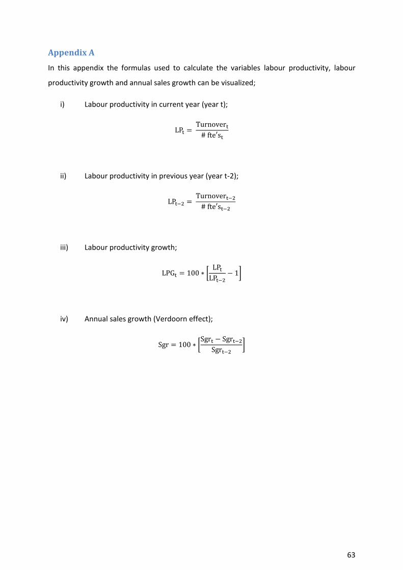
63

Appendix A

In this appendix the formulas used to calculate the variables labour productivity, labour

productivity growth and annual sales growth can be visualized;

i) Labour productivity in current year (year t);

ii) Labour productivity in previous year (year t-2);

iii) Labour productivity growth;

[

]

iv) Annual sales growth (Verdoorn effect);

[

]

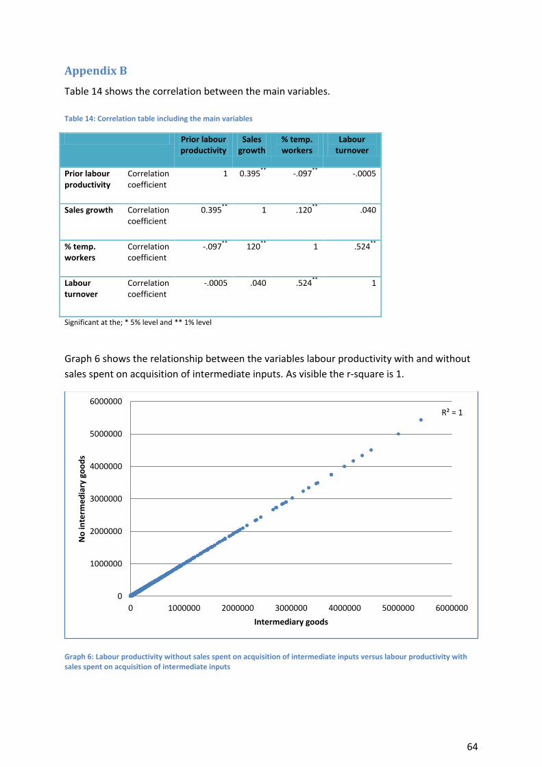
64

Appendix B

Table 14 shows the correlation between the main variables.

Table 14: Correlation table including the main variables

Prior labour productivity

Sales growth

% temp. workers

Labour turnover

Prior labour productivity

Correlation coefficient

1 0.395**

-.097**

-.0005

Sales growth Correlation coefficient

0.395**

1 .120**

.040

% temp. workers

Correlation coefficient

-.097**

120**

1 .524**

Labour turnover

Correlation coefficient

-.0005 .040 .524**

1

Significant at the; * 5% level and ** 1% level

Graph 6 shows the relationship between the variables labour productivity with and without

sales spent on acquisition of intermediate inputs. As visible the r-square is 1.

Graph 6: Labour productivity without sales spent on acquisition of intermediate inputs versus labour productivity with sales spent on acquisition of intermediate inputs

R² = 1

0

1000000

2000000

3000000

4000000

5000000

6000000

0 1000000 2000000 3000000 4000000 5000000 6000000

No

inte

rme

dia

ry g

oo

ds

Intermediary goods

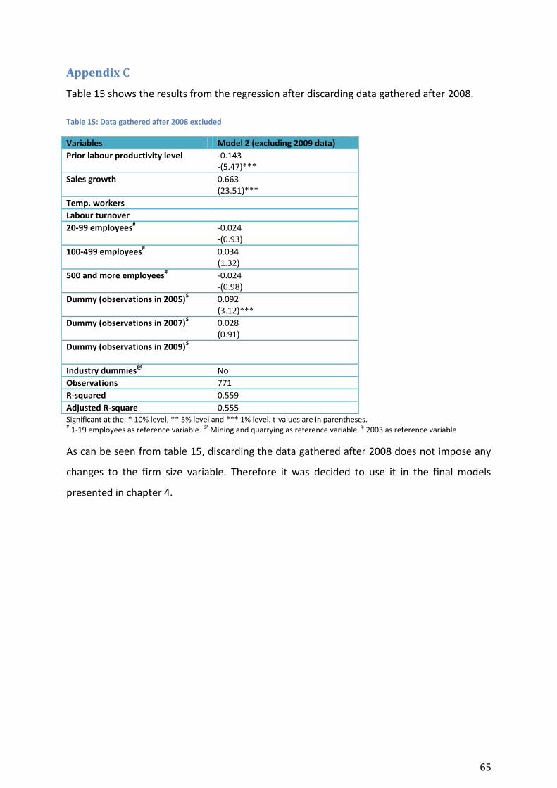
65

Appendix C

Table 15 shows the results from the regression after discarding data gathered after 2008.

Table 15: Data gathered after 2008 excluded

Variables Model 2 (excluding 2009 data)

Prior labour productivity level -0.143 -(5.47)***

Sales growth 0.663 (23.51)***

Temp. workers

Labour turnover

20-99 employees# -0.024

-(0.93)

100-499 employees# 0.034

(1.32)

500 and more employees# -0.024

-(0.98)

Dummy (observations in 2005)$

0.092 (3.12)***

Dummy (observations in 2007)$

0.028 (0.91)

Dummy (observations in 2009)$

Industry dummies@

No

Observations 771

R-squared 0.559

Adjusted R-square 0.555 Significant at the; * 10% level, ** 5% level and *** 1% level. t-values are in parentheses. # 1-19 employees as reference variable.

@ Mining and quarrying as reference variable.

$ 2003 as reference variable

As can be seen from table 15, discarding the data gathered after 2008 does not impose any

changes to the firm size variable. Therefore it was decided to use it in the final models

presented in chapter 4.

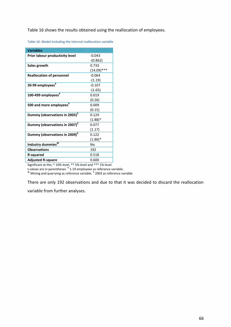
66

Table 16 shows the results obtained using the reallocation of employees.

Table 16: Model including the internal reallocation variable

Variables

Prior labour productivity level -0.043 -(0.862)

Sales growth 0.733 (14.09)***

Reallocation of personnel -0.064 -(1.19)

20-99 employees# -0.107

-(1.65)

100-499 employees# 0.019

(0.26)

500 and more employees# 0.009

(0.15)

Dummy (observations in 2005)$ 0.124

(1.88)*

Dummy (observations in 2007)$ 0.077

(1.17)

Dummy (observations in 2009)$ 0.122

(1.86)*

Industry dummies@

No

Observations 192

R-squared 0.518

Adjusted R-square 0.600 Significant at the; * 10% level, ** 5% level and *** 1% level. t-values are in parentheses.

# 1-19 employees as reference variable.

@ Mining and quarrying as reference variable.

$ 2003 as reference variable

There are only 192 observations and due to that it was decided to discard the reallocation

variable from further analyses.

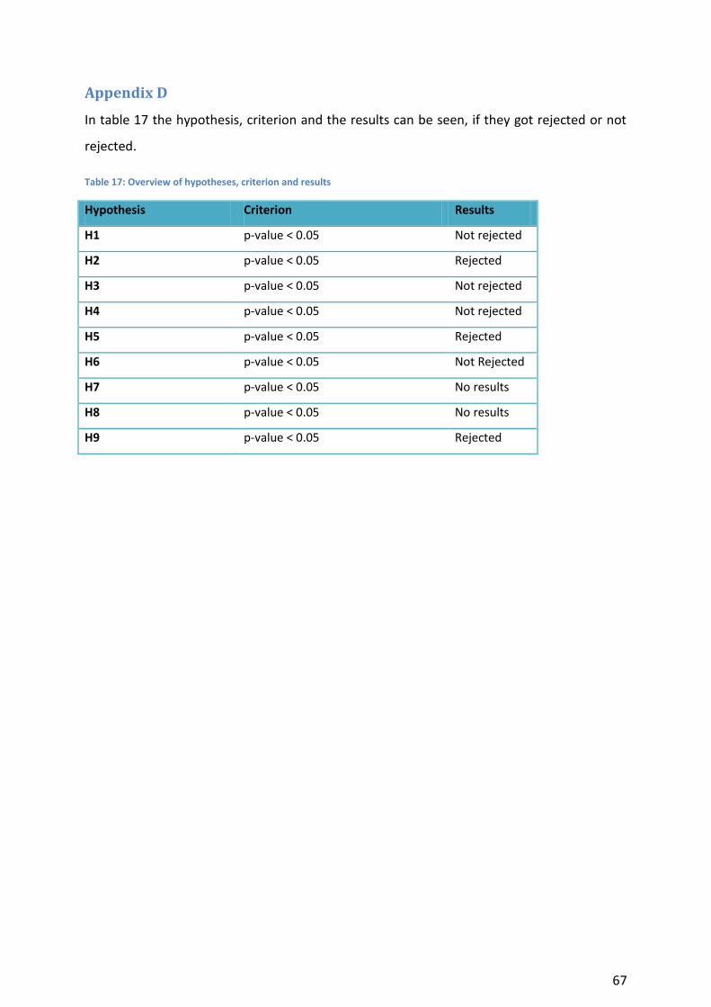
67

Appendix D

In table 17 the hypothesis, criterion and the results can be seen, if they got rejected or not

rejected.

Table 17: Overview of hypotheses, criterion and results

Hypothesis Criterion Results

H1 p-value < 0.05 Not rejected

H2 p-value < 0.05 Rejected

H3 p-value < 0.05 Not rejected

H4 p-value < 0.05 Not rejected

H5 p-value < 0.05 Rejected

H6 p-value < 0.05 Not Rejected

H7 p-value < 0.05 No results

H8 p-value < 0.05 No results

H9 p-value < 0.05 Rejected