Embed Size (px)
Citation preview
Islamic University-Gaza
Faculty of Science
Department of Physics
Laboratory Experiments in Optics
Prepared by
Zaher Nassar
and
Revised by
Dr. Hussian Dawoud
2007
Contents
1 Michelson Interferometer 6
1.1 Objective . . . . . . . . . . . . . . . . . . . . . . . . . . . . . . . . . . . . 6
1.2 Principle and Task . . . . . . . . . . . . . . . . . . . . . . . . . . . . . . . 6
1.3 Theory . . . . . . . . . . . . . . . . . . . . . . . . . . . . . . . . . . . . . . 6
1.3.1 Coherent sources . . . . . . . . . . . . . . . . . . . . . . . . . . . . 6
1.3.2 Composition of two simple harmonic motions in a straight line . . . 7
1.3.3 Michelson interferometer . . . . . . . . . . . . . . . . . . . . . . . . 8
1.4 Equipment . . . . . . . . . . . . . . . . . . . . . . . . . . . . . . . . . . . . 11
1.5 Setup and Procedure . . . . . . . . . . . . . . . . . . . . . . . . . . . . . . 11
1.5.1 Adjustment of the interferometer . . . . . . . . . . . . . . . . . . . 11
1.5.2 Measuring the wavelength of the laser light . . . . . . . . . . . . . . 12
1.6 Measurements and Calculations . . . . . . . . . . . . . . . . . . . . . . . . 12
2 Interference of Microwaves 14
2.1 Objective . . . . . . . . . . . . . . . . . . . . . . . . . . . . . . . . . . . . 14
2.2 Principle and Task . . . . . . . . . . . . . . . . . . . . . . . . . . . . . . . 14
2.3 Theory . . . . . . . . . . . . . . . . . . . . . . . . . . . . . . . . . . . . . . 14
2.3.1 Standing waves . . . . . . . . . . . . . . . . . . . . . . . . . . . . . 14
2.3.2 Interference of microwaves by using Michelson interferometer . . . . 16
2.4 Equipment . . . . . . . . . . . . . . . . . . . . . . . . . . . . . . . . . . . . 17
2.5 Setup and Procedure . . . . . . . . . . . . . . . . . . . . . . . . . . . . . . 18
2.5.1 Reflection at the metal plate (standing waves) . . . . . . . . . . . . 18
2.5.2 Interference of Microwaves in the Michelson Interferometer . . . . . 19
3 Diffraction of Microwaves 21
3.1 Objective . . . . . . . . . . . . . . . . . . . . . . . . . . . . . . . . . . . . 21
3.2 Principle and Task . . . . . . . . . . . . . . . . . . . . . . . . . . . . . . . 21
3.3 Theory . . . . . . . . . . . . . . . . . . . . . . . . . . . . . . . . . . . . . . 21
3.3.1 Fresnel’s assumptions and Fresnel’s zones . . . . . . . . . . . . . . . 21
3.3.2 Huygens’ principle . . . . . . . . . . . . . . . . . . . . . . . . . . . 22
3.3.3 Fresnel and Fraunhofer diffraction . . . . . . . . . . . . . . . . . . . 23
3.3.4 Fraunhofer diffraction at a single slit . . . . . . . . . . . . . . . . . 24
2
3.4 Equipment . . . . . . . . . . . . . . . . . . . . . . . . . . . . . . . . . . . . 27
3.5 Setup and Procedure . . . . . . . . . . . . . . . . . . . . . . . . . . . . . . 28
3.6 Measurements and calculations . . . . . . . . . . . . . . . . . . . . . . . . 29
4 Refraction Through Prism 30
4.1 Objective . . . . . . . . . . . . . . . . . . . . . . . . . . . . . . . . . . . . 30
4.2 Principle and Task . . . . . . . . . . . . . . . . . . . . . . . . . . . . . . . 30
4.3 Theory . . . . . . . . . . . . . . . . . . . . . . . . . . . . . . . . . . . . . . 30
4.3.1 Refraction Through a Prism . . . . . . . . . . . . . . . . . . . . . . 31
4.3.2 Minimum Deviation . . . . . . . . . . . . . . . . . . . . . . . . . . 31
4.3.3 The Spectrometer . . . . . . . . . . . . . . . . . . . . . . . . . . . . 32
4.3.4 Measurement of the angle A, of a prism . . . . . . . . . . . . . . . . 33
4.3.5 Measurement of the minimum deviation Dm . . . . . . . . . . . . . 34
4.4 Equipment . . . . . . . . . . . . . . . . . . . . . . . . . . . . . . . . . . . . 34
4.5 Set up and procedure . . . . . . . . . . . . . . . . . . . . . . . . . . . . . . 35
4.5.1 Determination of the refracting angle A . . . . . . . . . . . . . . . . 35
4.5.2 Determination of the angle of minimum deviation Dm . . . . . . . . 36
4.6 Measurements and calculations . . . . . . . . . . . . . . . . . . . . . . . . 37
5 Polarimetry 38
5.1 Objective . . . . . . . . . . . . . . . . . . . . . . . . . . . . . . . . . . . . 38
5.2 Principle and Task . . . . . . . . . . . . . . . . . . . . . . . . . . . . . . . 38
5.3 Theory . . . . . . . . . . . . . . . . . . . . . . . . . . . . . . . . . . . . . . 38
5.3.1 Polarization of light waves . . . . . . . . . . . . . . . . . . . . . . . 38
5.3.2 Optical activity . . . . . . . . . . . . . . . . . . . . . . . . . . . . . 39
5.3.3 Specific rotation . . . . . . . . . . . . . . . . . . . . . . . . . . . . . 39
5.3.4 Laurent’s polarimeter . . . . . . . . . . . . . . . . . . . . . . . . . . 40
5.4 Equipment . . . . . . . . . . . . . . . . . . . . . . . . . . . . . . . . . . . . 42
5.5 Set up and procedure . . . . . . . . . . . . . . . . . . . . . . . . . . . . . . 42
5.6 Measurements and calculations . . . . . . . . . . . . . . . . . . . . . . . . 44
6 Measuring the Velocity of Light 46
6.1 Objective . . . . . . . . . . . . . . . . . . . . . . . . . . . . . . . . . . . . 46
6.2 Principle and Task . . . . . . . . . . . . . . . . . . . . . . . . . . . . . . . 46
3
6.3 Theory . . . . . . . . . . . . . . . . . . . . . . . . . . . . . . . . . . . . . . 46
6.3.1 Composition of two simple harmonic motions acting at right angles 47
6.3.2 Velocity of light in air . . . . . . . . . . . . . . . . . . . . . . . . . 49
6.3.3 Velocity of light in medium . . . . . . . . . . . . . . . . . . . . . . 50
6.4 Equipment . . . . . . . . . . . . . . . . . . . . . . . . . . . . . . . . . . . . 51
6.5 Set up and procedure . . . . . . . . . . . . . . . . . . . . . . . . . . . . . . 51
6.5.1 Adjustment of the apparatus . . . . . . . . . . . . . . . . . . . . . . 52
6.5.2 Measuring the velocity of light in air . . . . . . . . . . . . . . . . . 52
6.5.3 Measuring the velocity of light in medium . . . . . . . . . . . . . . 53
7 Newton’s Rings 55
7.1 Objective . . . . . . . . . . . . . . . . . . . . . . . . . . . . . . . . . . . . 55
7.2 Principle and Task . . . . . . . . . . . . . . . . . . . . . . . . . . . . . . . 55
7.3 Theory . . . . . . . . . . . . . . . . . . . . . . . . . . . . . . . . . . . . . . 55
7.3.1 Newton’s rings by transmitted light . . . . . . . . . . . . . . . . . . 56
7.4 Equipment . . . . . . . . . . . . . . . . . . . . . . . . . . . . . . . . . . . . 58
7.5 Set up and procedure . . . . . . . . . . . . . . . . . . . . . . . . . . . . . . 58
7.6 Measurements and calculations . . . . . . . . . . . . . . . . . . . . . . . . 59
8 Specific charge of the electron - e/me 60
8.1 Objective . . . . . . . . . . . . . . . . . . . . . . . . . . . . . . . . . . . . 60
8.2 Principle and Task . . . . . . . . . . . . . . . . . . . . . . . . . . . . . . . 60
8.3 Theory . . . . . . . . . . . . . . . . . . . . . . . . . . . . . . . . . . . . . . 60
8.3.1 Deflection of the electron in magnetic field . . . . . . . . . . . . . . 60
8.3.2 Magnetic field on the axis of a circular coil . . . . . . . . . . . . . . 62
8.3.3 Helmholtz coils . . . . . . . . . . . . . . . . . . . . . . . . . . . . . 63
8.4 Equipment . . . . . . . . . . . . . . . . . . . . . . . . . . . . . . . . . . . . 63
8.5 Set up and procedure . . . . . . . . . . . . . . . . . . . . . . . . . . . . . . 63
8.6 Measurements and calculations . . . . . . . . . . . . . . . . . . . . . . . . 65
9 Diffraction grating 67
9.1 Objective . . . . . . . . . . . . . . . . . . . . . . . . . . . . . . . . . . . . 67
9.2 Principle and Task . . . . . . . . . . . . . . . . . . . . . . . . . . . . . . . 67
9.3 Theory . . . . . . . . . . . . . . . . . . . . . . . . . . . . . . . . . . . . . . 67
4
9.4 Fraunhofer diffraction at double slit . . . . . . . . . . . . . . . . . . . . . . 67
9.4.1 Interference maxima and minima . . . . . . . . . . . . . . . . . . . 68
9.4.2 Diffraction maxima and minima . . . . . . . . . . . . . . . . . . . . 70
9.4.3 Plane transmission diffraction grating . . . . . . . . . . . . . . . . . 70
9.4.4 Determination of the wave length of a spectral line using plane
transmission grating . . . . . . . . . . . . . . . . . . . . . . . . . . 71
9.5 Equipment . . . . . . . . . . . . . . . . . . . . . . . . . . . . . . . . . . . . 71
9.6 Set up and procedure . . . . . . . . . . . . . . . . . . . . . . . . . . . . . . 71
9.7 Measurements and calculations . . . . . . . . . . . . . . . . . . . . . . . . 73
10 Laws of lenses 75
10.1 Objective . . . . . . . . . . . . . . . . . . . . . . . . . . . . . . . . . . . . 75
10.2 Principle and Task . . . . . . . . . . . . . . . . . . . . . . . . . . . . . . . 75
10.3 Theory . . . . . . . . . . . . . . . . . . . . . . . . . . . . . . . . . . . . . . 75
10.3.1 Thin Lens Equation . . . . . . . . . . . . . . . . . . . . . . . . . . 75
10.3.2 Bessel’s method . . . . . . . . . . . . . . . . . . . . . . . . . . . . . 76
10.4 Equipment . . . . . . . . . . . . . . . . . . . . . . . . . . . . . . . . . . . . 77
10.5 Setup and Procedure . . . . . . . . . . . . . . . . . . . . . . . . . . . . . . 78
10.5.1 Determination of the focal length of an unknown convex lens by
using thin lens equation method . . . . . . . . . . . . . . . . . . . . 78
10.5.2 Determination of the focal length of a convex lens by using Bessel’s
method. . . . . . . . . . . . . . . . . . . . . . . . . . . . . . . . . . 79
10.6 Measurements and Calculations . . . . . . . . . . . . . . . . . . . . . . . . 79
5
1 Michelson Interferometer
1.1 Objective
Determination of the wave length of the light of the helium-neon laser by means of Michel-
son interferometer.
1.2 Principle and Task
Light is made to produce interference in the Michelson arrangement by the use of two
mirrors. The wave length is determined by displacing one mirror using the micrometer
screw.
1.3 Theory
The phenomenon of interference of light has proved the validity of the wave theory of
light. Interference is produced due to the superposition of two waves. It is not possible
to show interference due to two independent sources of light because a large number
of difficulties are involved. The two independent sources may emit light waves of largely
different amplitude and wavelength, and the phase difference between the two may change
with time.
1.3.1 Coherent sources
Two sources are said to be coherent if they emit light waves of the same frequency, nearly
the same amplitude and are always in phase with each other. It means that the two
sources must emit radiation of the same color (wavelength). In actual it is not possible
to have two independent sources which are coherent. But for experimental purpose, two
virtual sources formed from a single source can act as coherent sources. Interference of
light takes place between the waves by two methods:
1. From the real source and a virtual source.
2. From two virtual sources formed due to a single source.
In all such cases, the two sources will act, as if they are perfectly similar in all respects.
6
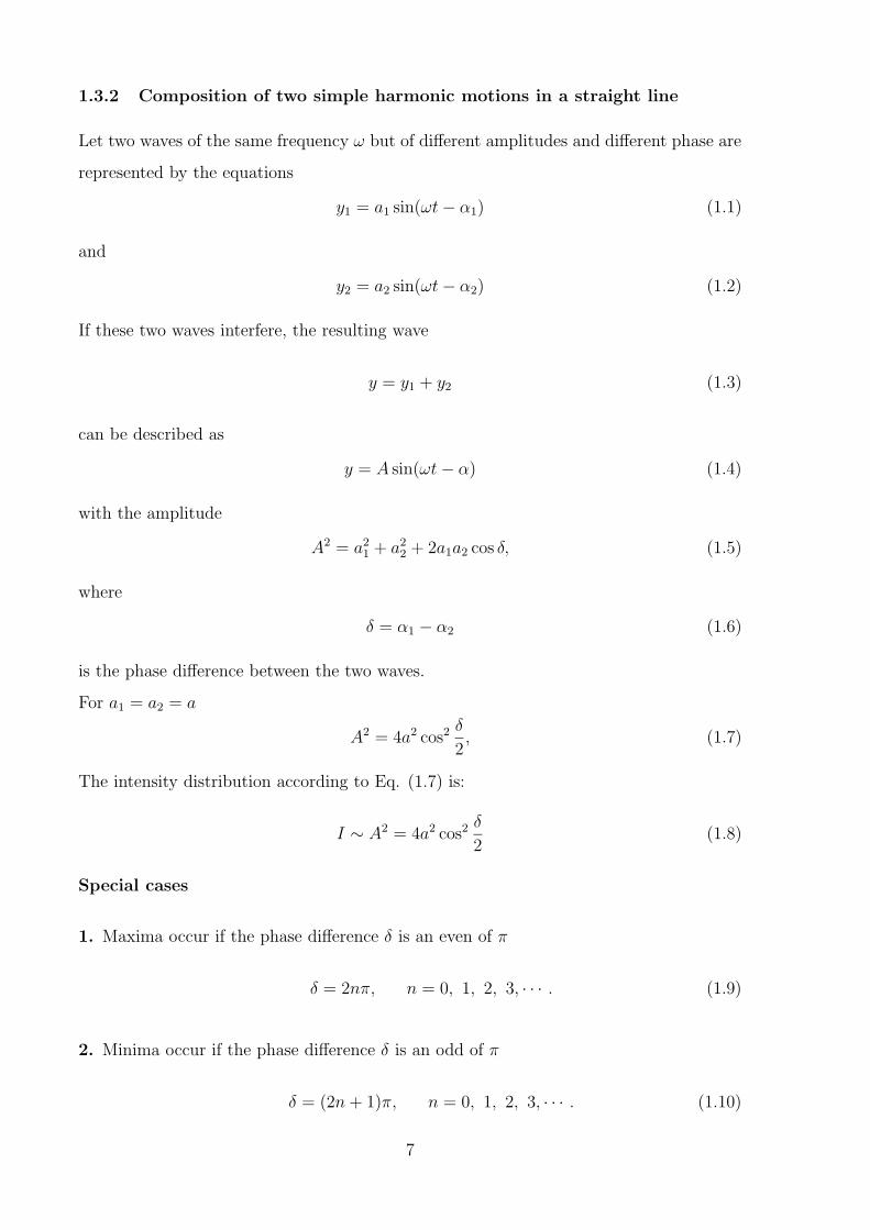
1.3.2 Composition of two simple harmonic motions in a straight line
Let two waves of the same frequency ω but of different amplitudes and different phase are
represented by the equations
y1 = a1 sin(ωt− α1) (1.1)
and
y2 = a2 sin(ωt− α2) (1.2)
If these two waves interfere, the resulting wave
y = y1 + y2 (1.3)
can be described as
y = A sin(ωt− α) (1.4)
with the amplitude
A2 = a21 + a2
2 + 2a1a2 cos δ, (1.5)
where
δ = α1 − α2 (1.6)
is the phase difference between the two waves.
For a1 = a2 = a
A2 = 4a2 cos2δ
2, (1.7)
The intensity distribution according to Eq. (1.7) is:
I ∼ A2 = 4a2 cos2δ
2(1.8)
Special cases
1. Maxima occur if the phase difference δ is an even of π
δ = 2nπ, n = 0, 1, 2, 3, · · · . (1.9)
2. Minima occur if the phase difference δ is an odd of π
δ = (2n+ 1)π, n = 0, 1, 2, 3, · · · . (1.10)
7
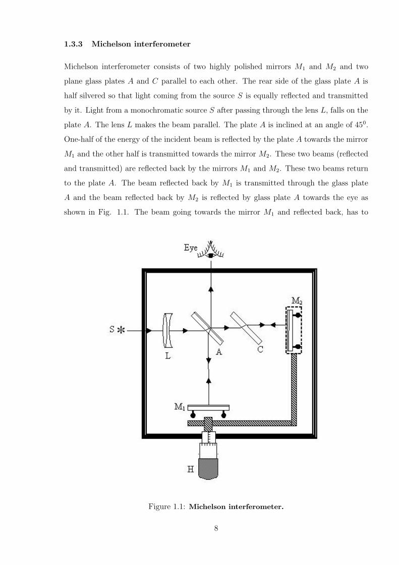
1.3.3 Michelson interferometer
Michelson interferometer consists of two highly polished mirrors M1 and M2 and two
plane glass plates A and C parallel to each other. The rear side of the glass plate A is
half silvered so that light coming from the source S is equally reflected and transmitted
by it. Light from a monochromatic source S after passing through the lens L, falls on the
plate A. The lens L makes the beam parallel. The plate A is inclined at an angle of 450.
One-half of the energy of the incident beam is reflected by the plate A towards the mirror
M1 and the other half is transmitted towards the mirror M2. These two beams (reflected
and transmitted) are reflected back by the mirrors M1 and M2. These two beams return
to the plate A. The beam reflected back by M1 is transmitted through the glass plate
A and the beam reflected back by M2 is reflected by glass plate A towards the eye as
shown in Fig. 1.1. The beam going towards the mirror M1 and reflected back, has to
Figure 1.1: Michelson interferometer.
8
pass twice through the glass plate A. Therefore, to compensate for the path, the plate C
is used between the mirror M2 and A. The light beam going towards the mirror M2 and
reflected back towards A also passes twice through the compensating plate C. Therefore,
the paths of the two rays in glass are the same. The mirror M2 can be moved with the
help of the micrometer handle H. The distance through which the mirror M2 is moved
can be read on the scale of the micrometer. The planes of the mirrors M1 and M2 can be
made perfectly perpendicular with the help of the fine screws attached to them.
• Remark
The compensating plate C is a necessity for white light fringes but can be dispensed with,
while using monochromatic light.
If the mirrors M1 and M2 are perfectly perpendicular, the observer’s eye will see the
images of the mirrors M1 and M2 through A. There will be an air film between the two
images and distance can be varied with the help of the micrometer handle H. The fringes
will be perfectly circular. If the two images ofM1 andM2 are inclined (the mirrorsM1 and
M2 not perfectly perpendicular) the enclosed air film will be wedge-shaped and straight
line fringes will be observed. When the mirror M2 is moved away or towards the glass
plate A with the help of handle H, the fringes cross the center of the field of view of the
observer’s eye. If M2 is moved through a distance λ/2, one fringe will cross the field of
view and will move to the position previously occupied by the next fringe.
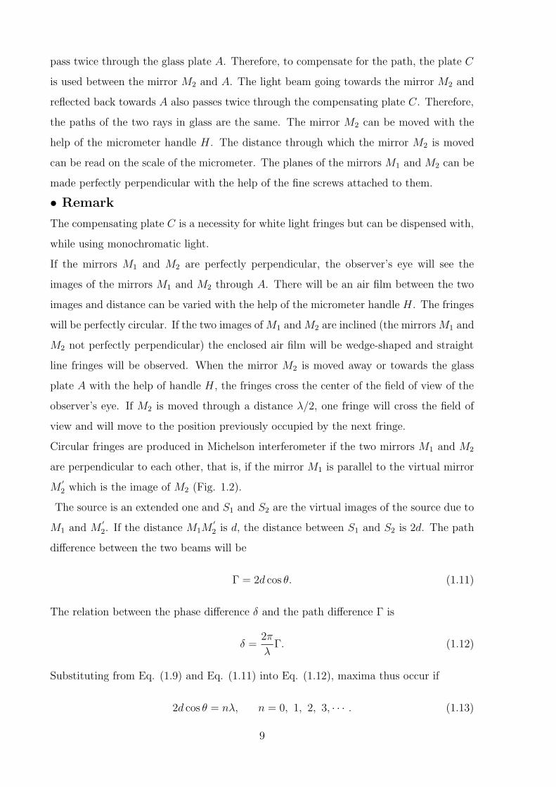
Circular fringes are produced in Michelson interferometer if the two mirrors M1 and M2
are perpendicular to each other, that is, if the mirror M1 is parallel to the virtual mirror
M′
2 which is the image of M2 (Fig. 1.2).
The source is an extended one and S1 and S2 are the virtual images of the source due to
M1 and M′
2. If the distance M1M′
2 is d, the distance between S1 and S2 is 2d. The path
difference between the two beams will be
Γ = 2d cos θ. (1.11)
The relation between the phase difference δ and the path difference Γ is
δ =2π
λΓ. (1.12)
Substituting from Eq. (1.9) and Eq. (1.11) into Eq. (1.12), maxima thus occur if
2d cos θ = nλ, n = 0, 1, 2, 3, · · · . (1.13)
9
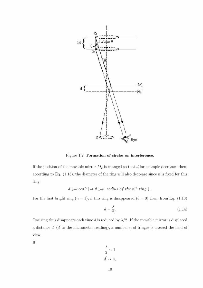
Figure 1.2: Formation of circles on interference.
If the position of the movable mirror M2 is changed so that d for example decreases then,
according to Eq. (1.13), the diameter of the ring will also decrease since n is fixed for this
ring:
d ↓⇒ cos θ ↑⇒ θ ↓⇒ radius of the nth ring ↓ .
For the first bright ring (n = 1), if this ring is disappeared (θ = 0) then, from Eq. (1.13)
d =λ
2. (1.14)
One ring thus disappears each time d is reduced by λ/2. If the movable mirror is displaced
a distance d′
(d′
is the micrometer reading), a number n of fringes is crossed the field of
view.
Ifλ
2∼ 1
d′
∼ n,
10
then
d′
= nλ
2(1.15)
or
2d′ = nλ. (1.16)
1.4 Equipment
Support base, helium-neon lazer, Michelson interferometer, screen.
1.5 Setup and Procedure
The experimental set up is as shown in Fig.1.3. In order to obtain the largest possi-
Figure 1.3: Experimental set-up for measuring wavelengths with the Michelson in-
terferometer.
ble number of interference fringes, the two mirrors of the interferometer are first of all
adjusted.
1.5.1 Adjustment of the interferometer
1. The laser beam is adjusted to strike the half-silvered mirror at an angle of 45◦.
11
2. The laser beam is split into two beams.
3. The resulting two beams are reflected by the mirrors and impinge on the screen.
4. Two points are obtained on the screen.
5. By means of the two adjusting screws, both points of light are made to coincide.
6. The points of light are enlarged and interference patterns are observed on the screen
(bands, circles).
7. By careful readjustment, an interference image of concentric circles can be obtained.
1.5.2 Measuring the wavelength of the laser light
1. The micrometer screw is turned to any initial position at which the center of the
circles is dark.
2. The initial reading of the micrometer is read.
3. The micrometer screws is now further turned in the same direction and 40 light-dark
periods are counted.
4. The distance travelled by the mirror must be read on the micrometer screw and
divided by ten (when the micrometer screw moves 10 mm the mirror is displaced
1 mm ).
5. If the central point of the circles moves outside the light spot area, a readjustment
has to be performed in order to obtain concentric fringes.
17. Repeat paragraphs 13-16 for 60, 80, 100, 120, 140,160 and 180 circles.
18. Record your measurements in Table 1.1.
1.6 Measurements and Calculations
• Plot n as x-axis versus d′
as y-axis.
• Find the slope, then calculate the wavelength λ from Eq. (1.15) where
λ = 2 slope.
12
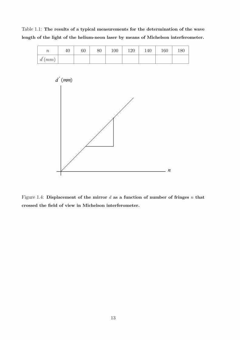
Table 1.1: The results of a typical measurements for the determination of the wave
length of the light of the helium-neon laser by means of Michelson interferometer.
n 40 60 80 100 120 140 160 180
d′
(mm)
Figure 1.4: Displacement of the mirror d as a function of number of fringes n that
crossed the field of view in Michelson interferometer.
13
2 Interference of Microwaves
2.1 Objective
Measurement of the wavelength of microwaves through the production of standing waves
with
1. reflection at the metal screen.
2. the Michelson interferometer.
2.2 Principle and Task
If a microwave beam is incident on a metal screen or glass plate, it will reflect and
interferes with the primary waves. The result of interference is said to be standing wave.
The wavelength of the microwave is determined from the resultant standing waves.
2.3 Theory
Interference of microwaves can take place by two methods:
1. Due to the superposition of the incident wave and reflected wave (standing waves).
2. Due to the superposition of two coherent virtual waves (Michelson interferometer).
2.3.1 Standing waves
Electromagnetic waves can be reflected; a conducting surface can serve as a reflector. The
superposition principle holds for electromagnetic waves just as for electric and magnetic
fields. The superposition of an incident wave and a perfectly reflected wave forms a
standing wave. The situation is analogous to standing waves on a stretched string.
We can derive a wave function for the standing wave by adding the functions for two waves
with equal amplitude, period and wave length, traveling in opposite directions. Call these
two wave functions E1 and E2.
Suppose E1 is the incident wave traveling to the left and described by the wave function
E1 = A sin(ωt+ kx), (2.1)
14
and E2 is the reflected wave traveling to the right and described by the wave function
E2 = −A sin(ωt− kx), (2.2)
where A is the amplitude of the wave, ω = 2πf is the angular frequency and k = 2π/λ is
the propagation constant.
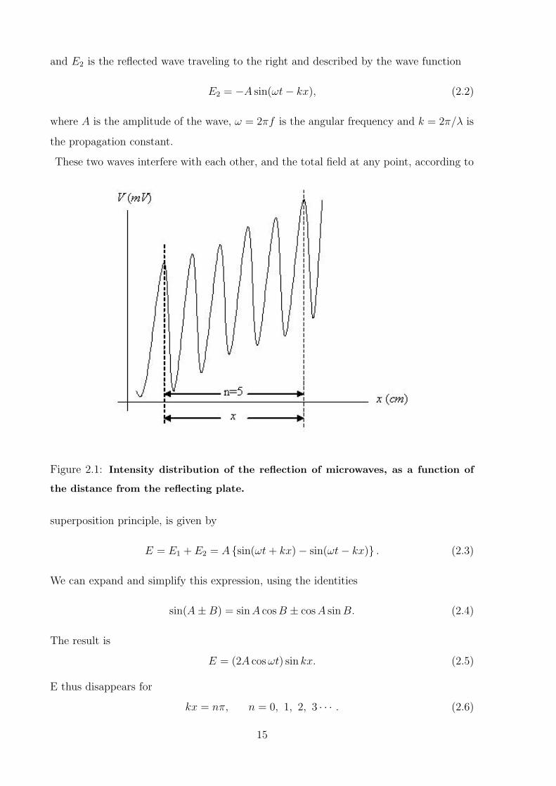
These two waves interfere with each other, and the total field at any point, according to
Figure 2.1: Intensity distribution of the reflection of microwaves, as a function of
the distance from the reflecting plate.
superposition principle, is given by
E = E1 + E2 = A {sin(ωt+ kx)− sin(ωt− kx)} . (2.3)
We can expand and simplify this expression, using the identities
sin(A±B) = sinA cosB ± cosA sinB. (2.4)
The result is
E = (2A cosωt) sin kx. (2.5)
E thus disappears for
kx = nπ, n = 0, 1, 2, 3 · · · . (2.6)
15
Since
k =2π
λ, (2.7)
then
x = n ·λ
2, n = 1, 2, 3 · · · (2.8)
From the distance between the maxima in Fig. 2.1, the wavelength can be calculated
using Eq. (2.8).
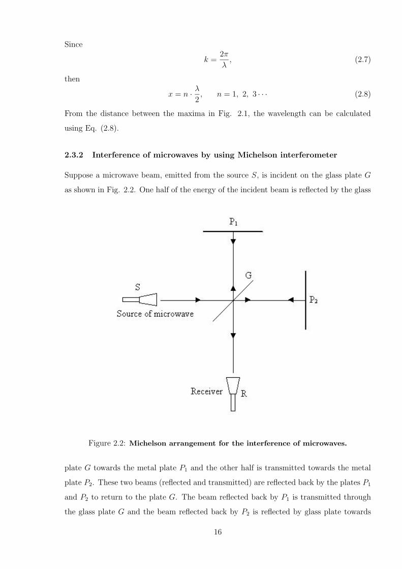
2.3.2 Interference of microwaves by using Michelson interferometer
Suppose a microwave beam, emitted from the source S, is incident on the glass plate G
as shown in Fig. 2.2. One half of the energy of the incident beam is reflected by the glass
Figure 2.2: Michelson arrangement for the interference of microwaves.
plate G towards the metal plate P1 and the other half is transmitted towards the metal
plate P2. These two beams (reflected and transmitted) are reflected back by the plates P1
and P2 to return to the plate G. The beam reflected back by P1 is transmitted through
the glass plate G and the beam reflected back by P2 is reflected by glass plate towards
16
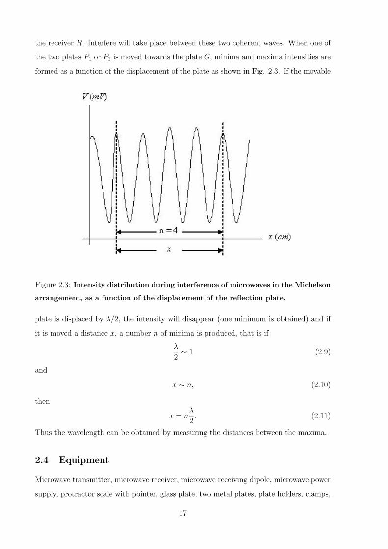
the receiver R. Interfere will take place between these two coherent waves. When one of
the two plates P1 or P2 is moved towards the plate G, minima and maxima intensities are
formed as a function of the displacement of the plate as shown in Fig. 2.3. If the movable
Figure 2.3: Intensity distribution during interference of microwaves in the Michelson
arrangement, as a function of the displacement of the reflection plate.
plate is displaced by λ/2, the intensity will disappear (one minimum is obtained) and if
it is moved a distance x, a number n of minima is produced, that is if
λ
2∼ 1 (2.9)
and
x ∼ n, (2.10)
then
x = nλ
2. (2.11)
Thus the wavelength can be obtained by measuring the distances between the maxima.
2.4 Equipment
Microwave transmitter, microwave receiver, microwave receiving dipole, microwave power
supply, protractor scale with pointer, glass plate, two metal plates, plate holders, clamps,
17
meter scale, tripod base, support rod, multimeter and connecting cable.
2.5 Setup and Procedure
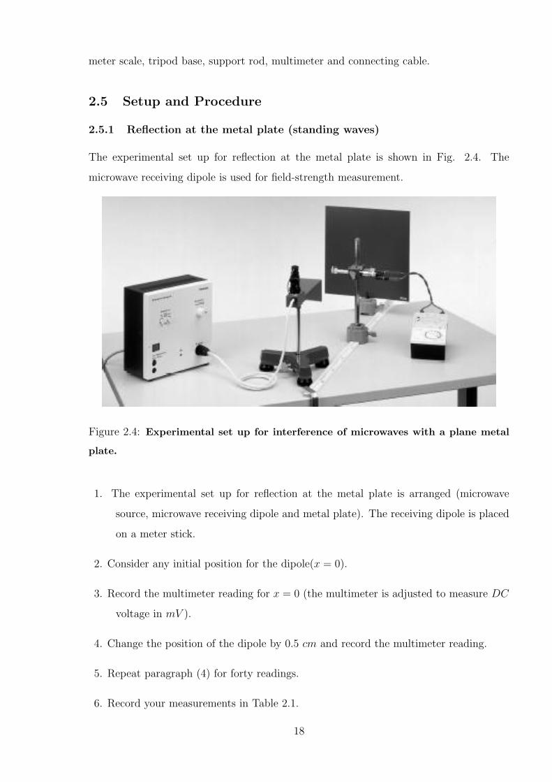
2.5.1 Reflection at the metal plate (standing waves)
The experimental set up for reflection at the metal plate is shown in Fig. 2.4. The
microwave receiving dipole is used for field-strength measurement.
Figure 2.4: Experimental set up for interference of microwaves with a plane metal
plate.
1. The experimental set up for reflection at the metal plate is arranged (microwave
source, microwave receiving dipole and metal plate). The receiving dipole is placed
on a meter stick.
2. Consider any initial position for the dipole(x = 0).
3. Record the multimeter reading for x = 0 (the multimeter is adjusted to measure DC
voltage in mV ).
4. Change the position of the dipole by 0.5 cm and record the multimeter reading.
5. Repeat paragraph (4) for forty readings.
6. Record your measurements in Table 2.1.
18
7. Plot the voltage V (mv) as y-axis versus the displacement x(cm) as x axis.
8. Measure the distance x between two maxima and count the number of minima n
within the distance x as shown in Fig. 2.1.
9. calculate the wave length of the microwave from Eq. (2.8).
Table 2.1: The results of a typical measurements for the determination of the wave
length of the microwave by means of reflection on the metal plate.
x(cm) 0 0.5 1 1.5 2 2.5 3 3.5 4 4.5 .... .... .... .... 20
V (mv)
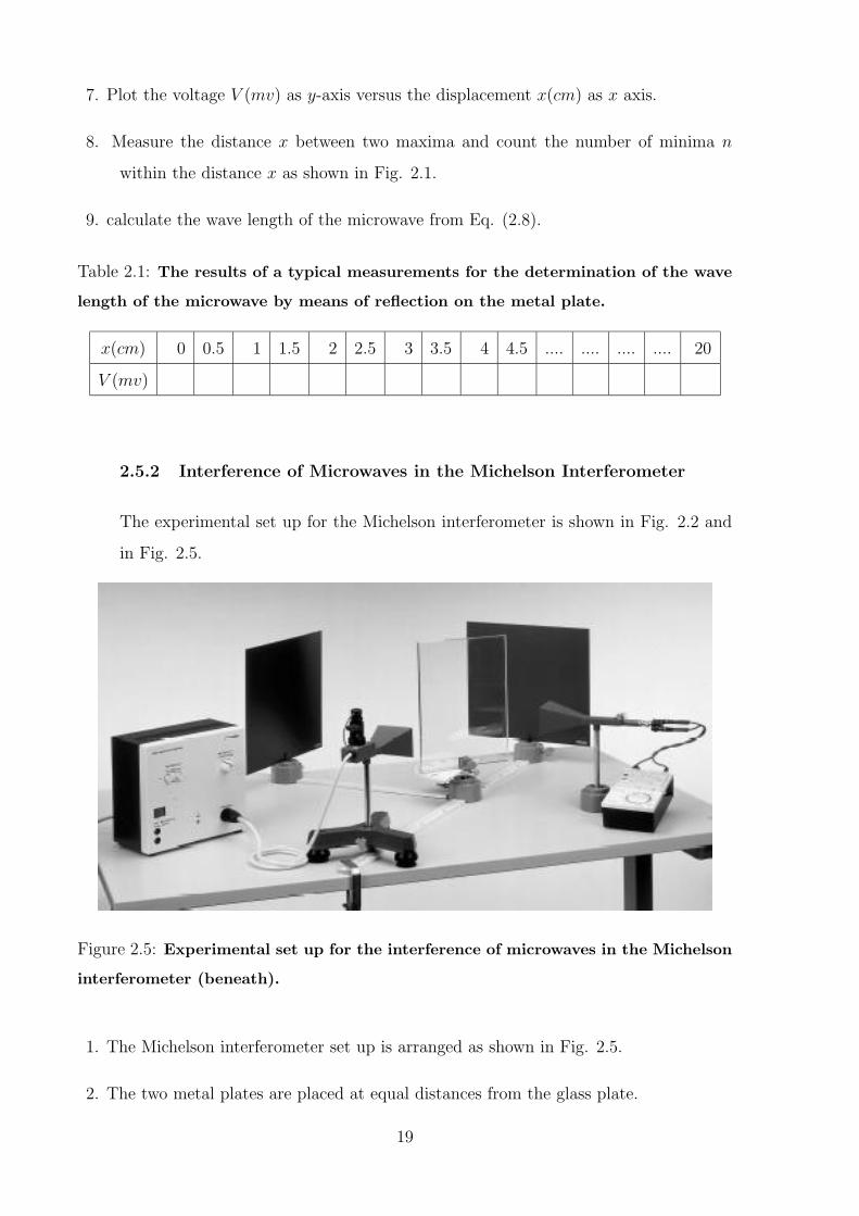
2.5.2 Interference of Microwaves in the Michelson Interferometer
The experimental set up for the Michelson interferometer is shown in Fig. 2.2 and
in Fig. 2.5.
Figure 2.5: Experimental set up for the interference of microwaves in the Michelson
interferometer (beneath).
1. The Michelson interferometer set up is arranged as shown in Fig. 2.5.
2. The two metal plates are placed at equal distances from the glass plate.
19
3. Consider the position of one of the metal plates to have the coordinate x = 0.
4. Record the multimeter reading for x = 0.
5. Displace the metal plate by 0.5 cm and record the multimeter reading.
6. Repeat paragraph (5) for forty readings.
7. Record your measurements in Table 2.2.
8. Plot the voltage V (mv) as y-axis versus the displacement x(cm) as x axis.
9. Measure the distance x between two maxima and count the number of minima n
within the distance x as shown in Fig. 2.1.
10. calculate the wave length of the microwave from Eq. (2.11).
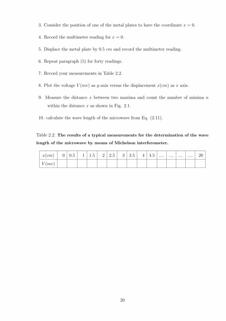
Table 2.2: The results of a typical measurements for the determination of the wave
length of the microwave by means of Michelson interferometer.
x(cm) 0 0.5 1 1.5 2 2.5 3 3.5 4 4.5 .... .... .... .... 20
V (mv)
20
3 Diffraction of Microwaves
3.1 Objective
Determination of the diffraction pattern of the microwave intensity after passing through
a slit.
3.2 Principle and Task
Microwaves impinge on a slit. The diffraction pattern is determined on the basis of
diffraction at this slit.
3.3 Theory
If an opaque obstacle is placed in the path of light, a sharp shadow is cast on the screen,
indicating thereby that light travels in straight lines. But it has observed that when a
beam of light passes through a small opening (a small circular hole or a narrow slit) it
spreads to some extent into the region of the geometrical shadow also. If light energy is
propagated in the form of waves, then similar to sound waves one would expect bending of
the beam of light round the edges of an opaque obstacle or illumination of the geometrical
shadow. The bending of light round the edges of an obstacle or the encroachment of light
within the geometrical shadow is called diffraction.
3.3.1 Fresnel’s assumptions and Fresnel’s zones
According to Fresnel, the resultant effect at an external point due to a wavefront will
depend on the factors discussed below:
In Fig. 3.1, S is a point source of monochromatic light, MN is a small aperture and XY
is the screen. MCN is the incident spherical wave front due to the point source S. To
obtain the resultant effect at a point P on the screen, Fresnel assumed that:
1. A wavefront can be divided into a large number of strips or zones called Fresnel’s zones
of small area and the resultant effect at any point will depend on the combined effect
of all the secondary waves emanating from the various zones.
2. the effect at a point due to any particular zone will depend on the distance of the point
from the zone.
21
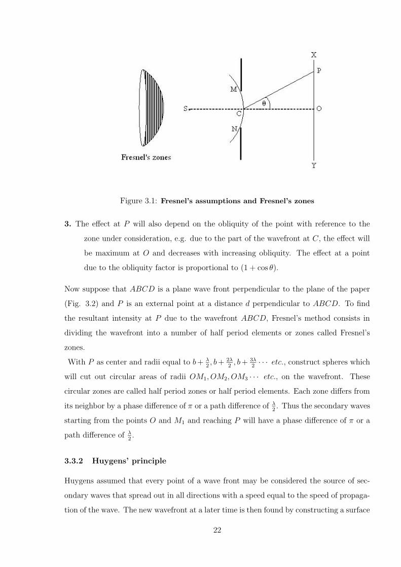
Figure 3.1: Fresnel’s assumptions and Fresnel’s zones
3. The effect at P will also depend on the obliquity of the point with reference to the
zone under consideration, e.g. due to the part of the wavefront at C, the effect will
be maximum at O and decreases with increasing obliquity. The effect at a point
due to the obliquity factor is proportional to (1 + cos θ).
Now suppose that ABCD is a plane wave front perpendicular to the plane of the paper
(Fig. 3.2) and P is an external point at a distance d perpendicular to ABCD. To find
the resultant intensity at P due to the wavefront ABCD, Fresnel’s method consists in
dividing the wavefront into a number of half period elements or zones called Fresnel’s
zones.
With P as center and radii equal to b+ λ2, b+ 2λ
2, b+ 3λ
2· · · etc., construct spheres which
will cut out circular areas of radii OM1, OM2, OM3 · · · etc., on the wavefront. These
circular zones are called half period zones or half period elements. Each zone differs from
its neighbor by a phase difference of π or a path difference of λ2. Thus the secondary waves
starting from the points O and M1 and reaching P will have a phase difference of π or a
path difference of λ2.
3.3.2 Huygens’ principle
Huygens assumed that every point of a wave front may be considered the source of sec-
ondary waves that spread out in all directions with a speed equal to the speed of propaga-
tion of the wave. The new wavefront at a later time is then found by constructing a surface
22
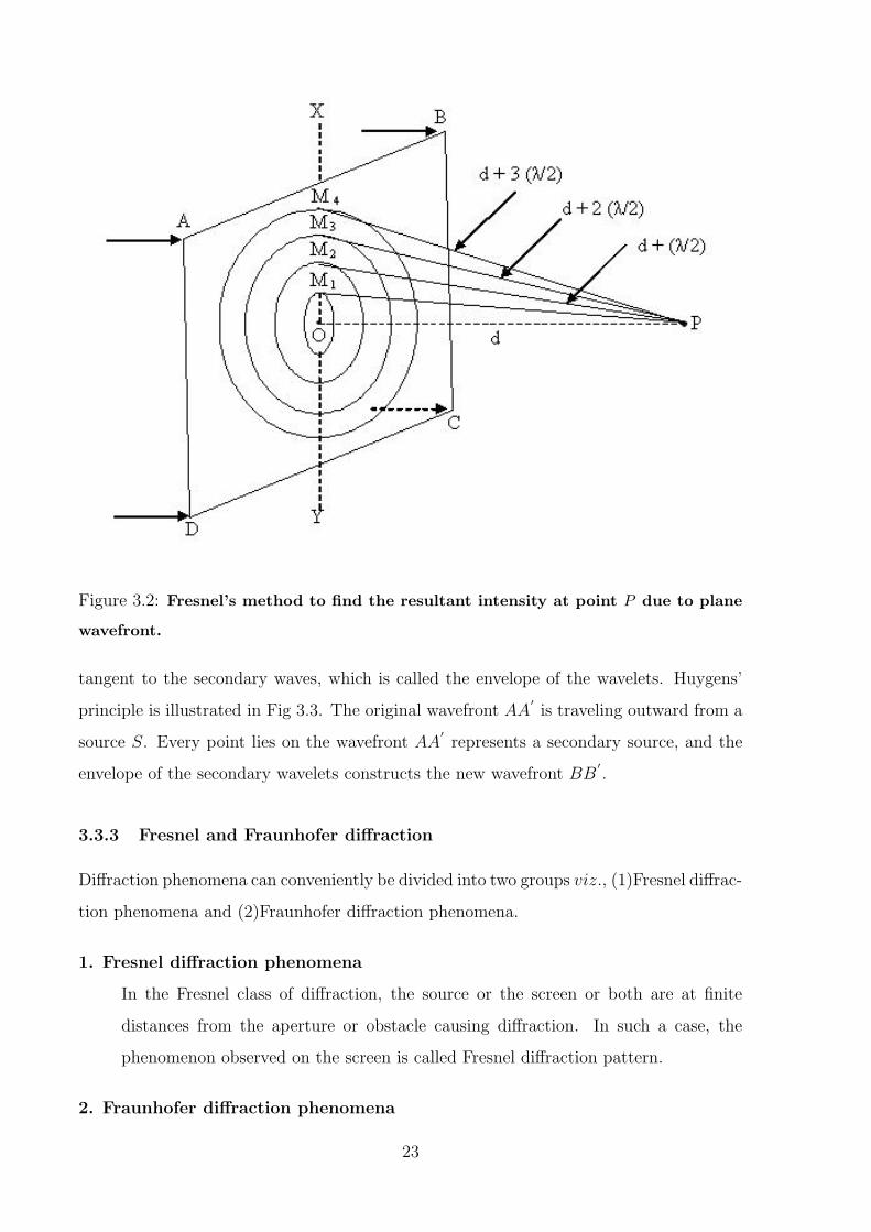
Figure 3.2: Fresnel’s method to find the resultant intensity at point P due to plane
wavefront.
tangent to the secondary waves, which is called the envelope of the wavelets. Huygens’
principle is illustrated in Fig 3.3. The original wavefront AA′
is traveling outward from a
source S. Every point lies on the wavefront AA′
represents a secondary source, and the
envelope of the secondary wavelets constructs the new wavefront BB′
.
3.3.3 Fresnel and Fraunhofer diffraction
Diffraction phenomena can conveniently be divided into two groups viz., (1)Fresnel diffrac-
tion phenomena and (2)Fraunhofer diffraction phenomena.
1. Fresnel diffraction phenomena
In the Fresnel class of diffraction, the source or the screen or both are at finite
distances from the aperture or obstacle causing diffraction. In such a case, the
phenomenon observed on the screen is called Fresnel diffraction pattern.
2. Fraunhofer diffraction phenomena
23
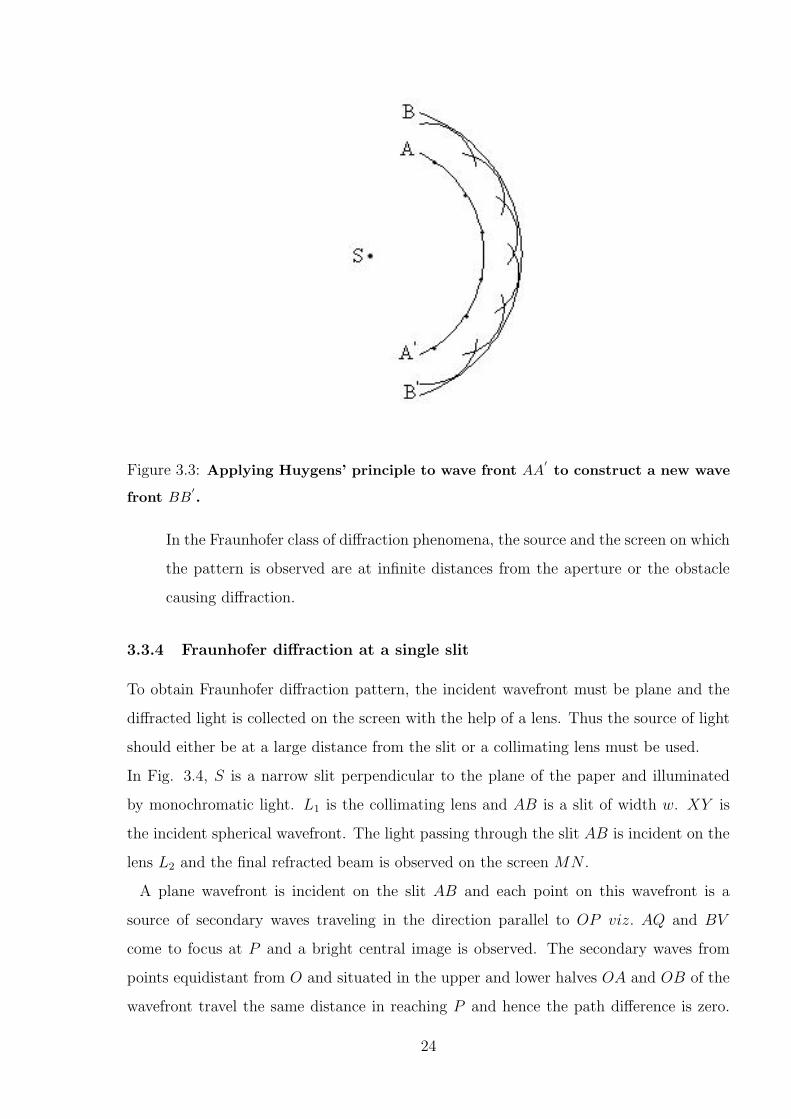
Figure 3.3: Applying Huygens’ principle to wave front AA′to construct a new wave
front BB′.
In the Fraunhofer class of diffraction phenomena, the source and the screen on which
the pattern is observed are at infinite distances from the aperture or the obstacle
causing diffraction.
3.3.4 Fraunhofer diffraction at a single slit
To obtain Fraunhofer diffraction pattern, the incident wavefront must be plane and the
diffracted light is collected on the screen with the help of a lens. Thus the source of light
should either be at a large distance from the slit or a collimating lens must be used.
In Fig. 3.4, S is a narrow slit perpendicular to the plane of the paper and illuminated
by monochromatic light. L1 is the collimating lens and AB is a slit of width w. XY is
the incident spherical wavefront. The light passing through the slit AB is incident on the
lens L2 and the final refracted beam is observed on the screen MN .
A plane wavefront is incident on the slit AB and each point on this wavefront is a
source of secondary waves traveling in the direction parallel to OP viz. AQ and BV
come to focus at P and a bright central image is observed. The secondary waves from
points equidistant from O and situated in the upper and lower halves OA and OB of the
wavefront travel the same distance in reaching P and hence the path difference is zero.
24
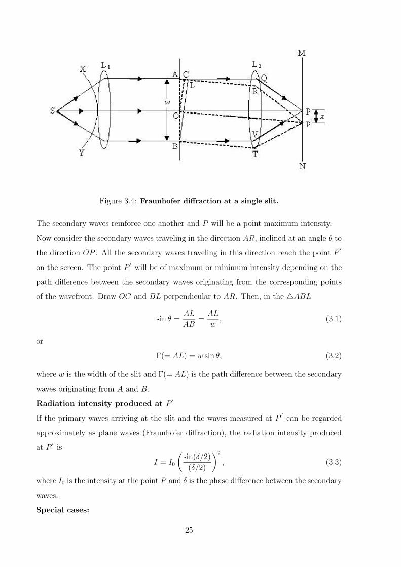
Figure 3.4: Fraunhofer diffraction at a single slit.
The secondary waves reinforce one another and P will be a point maximum intensity.
Now consider the secondary waves traveling in the direction AR, inclined at an angle θ to
the direction OP . All the secondary waves traveling in this direction reach the point P′
on the screen. The point P′
will be of maximum or minimum intensity depending on the
path difference between the secondary waves originating from the corresponding points
of the wavefront. Draw OC and BL perpendicular to AR. Then, in the 4ABL
sin θ =AL
AB=AL
w, (3.1)
or
Γ(= AL) = w sin θ, (3.2)
where w is the width of the slit and Γ(= AL) is the path difference between the secondary
waves originating from A and B.
Radiation intensity produced at P′
If the primary waves arriving at the slit and the waves measured at P′
can be regarded
approximately as plane waves (Fraunhofer diffraction), the radiation intensity produced
at P′
is
I = I0
(
sin(δ/2)
(δ/2)
)2
, (3.3)
where I0 is the intensity at the point P and δ is the phase difference between the secondary
waves.
Special cases:
25
1. Intensity is minimum when the phase difference δ is an even number multiple of π,
i.e., when
δ = 2nπ, n = 1, 2, 3 · · · . (3.4)
∵ δ =2π
λΓ, (3.5)
2nπ =2π
λΓ, (3.6)
∴ Γ = nλ. (3.7)
Thus, destructive interference takes place when the path difference is an integer
multiple of λ, and the point P′
will be of minimum intensity.
Equating Eq. (3.2) and Eq. (3.7) we can write
sin θn =nλ
w, n = 1, 2, 3 · · · , (3.8)
where θn gives the direction of the nth minimum.
2. Intensity is maximum when the phase difference δ is an odd number multiple of π, i.e.,
when
δ = (2n+ 1)π, n = 1, 2, 3 · · · . (3.9)
Similarly, we can show that a constructive interference takes place when the path
difference is an odd multiple of λ2, i.e., when
Γ =(2n+ 1)
2λ, n = 1, 2, 3 · · · , (3.10)
and the point P′
will be of maximum intensity.
Equating Eq. (3.2) and Eq. (3.10) gives
sin θn =(2n+ 1)λ
2w, n = 1, 2, 3 · · · , (3.11)
where θn gives the direction of the nth maximum.
Thus, the diffraction pattern due to a single slit consists of a central bright maximum at
P followed by secondary maxima and minima on both the sides as shown in Fig. 3.5.
If the lens L2 is very near the slit or the screen is far away from the lens L2, then
sin θn =xnf
=xnd, (3.12)
26
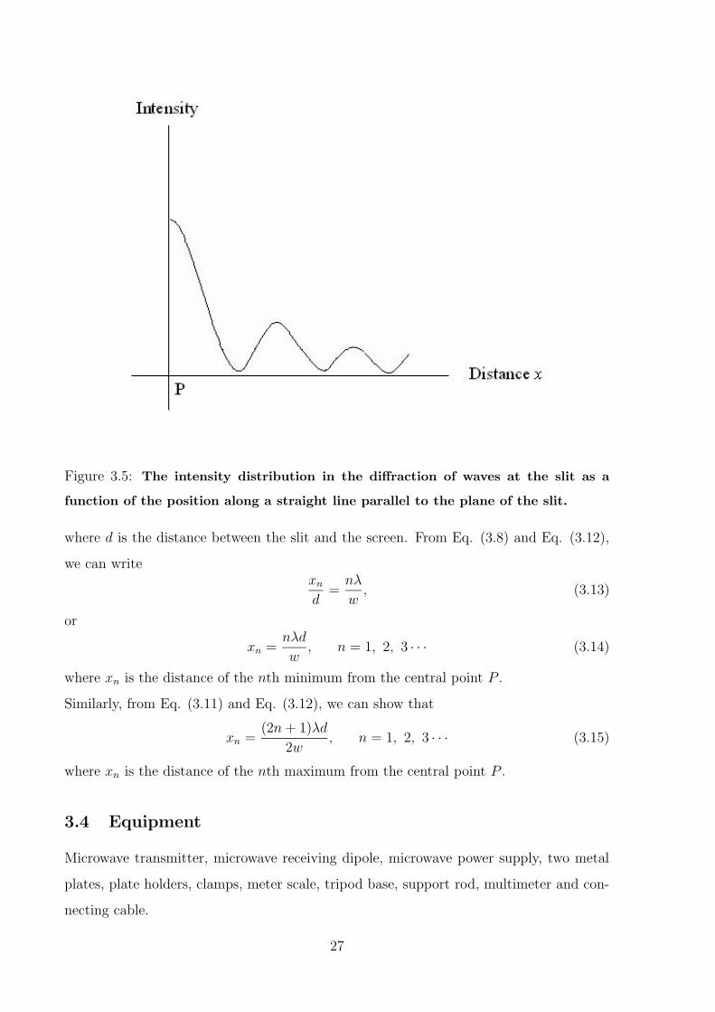
Figure 3.5: The intensity distribution in the diffraction of waves at the slit as a
function of the position along a straight line parallel to the plane of the slit.
where d is the distance between the slit and the screen. From Eq. (3.8) and Eq. (3.12),
we can writexnd
=nλ
w, (3.13)
or
xn =nλd
w, n = 1, 2, 3 · · · (3.14)
where xn is the distance of the nth minimum from the central point P .
Similarly, from Eq. (3.11) and Eq. (3.12), we can show that
xn =(2n+ 1)λd
2w, n = 1, 2, 3 · · · (3.15)
where xn is the distance of the nth maximum from the central point P .
3.4 Equipment
Microwave transmitter, microwave receiving dipole, microwave power supply, two metal
plates, plate holders, clamps, meter scale, tripod base, support rod, multimeter and con-
necting cable.
27
3.5 Setup and Procedure
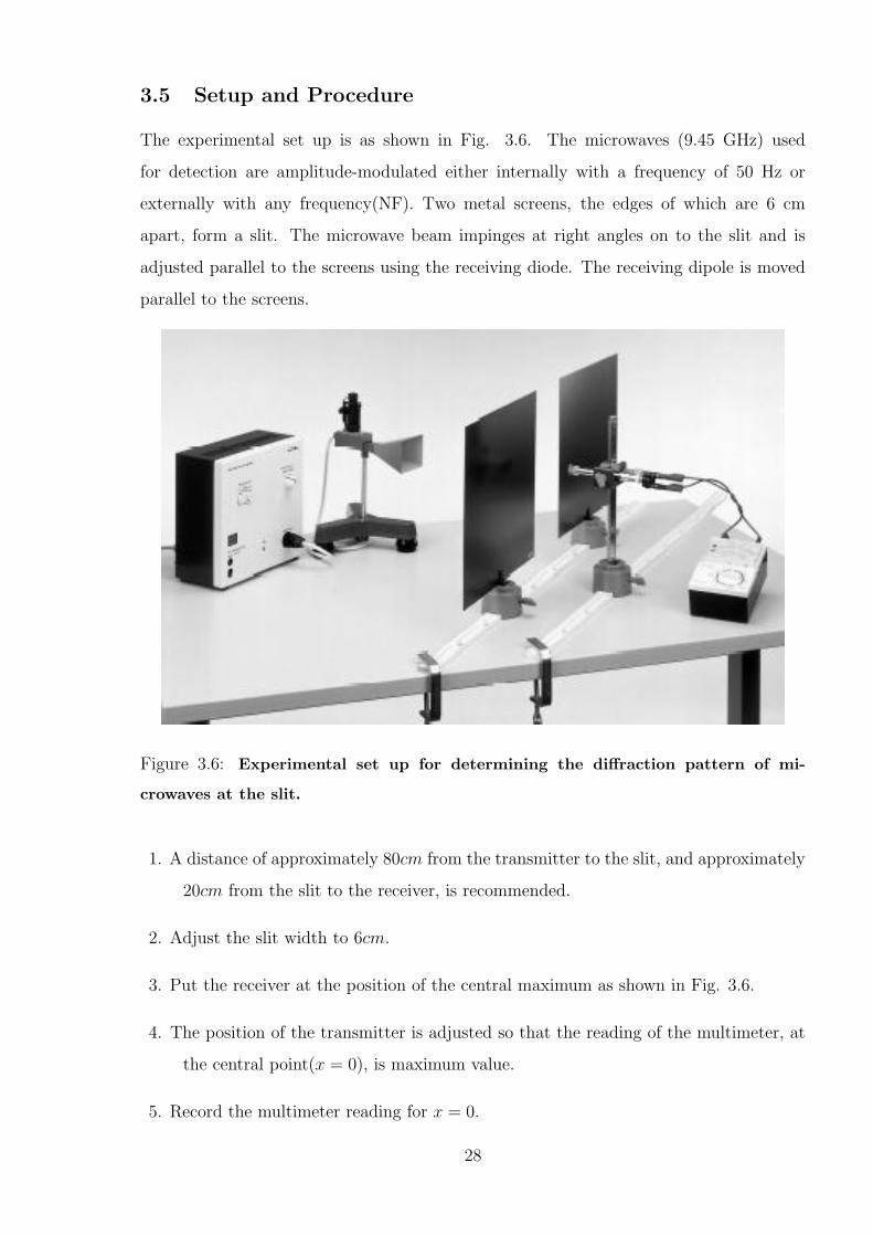
The experimental set up is as shown in Fig. 3.6. The microwaves (9.45 GHz) used
for detection are amplitude-modulated either internally with a frequency of 50 Hz or
externally with any frequency(NF). Two metal screens, the edges of which are 6 cm
apart, form a slit. The microwave beam impinges at right angles on to the slit and is
adjusted parallel to the screens using the receiving diode. The receiving dipole is moved
parallel to the screens.
Figure 3.6: Experimental set up for determining the diffraction pattern of mi-
crowaves at the slit.
1. A distance of approximately 80cm from the transmitter to the slit, and approximately
20cm from the slit to the receiver, is recommended.
2. Adjust the slit width to 6cm.
3. Put the receiver at the position of the central maximum as shown in Fig. 3.6.
4. The position of the transmitter is adjusted so that the reading of the multimeter, at
the central point(x = 0), is maximum value.
5. Record the multimeter reading for x = 0.
28
6. Change the position of the dipole by 0.5 cm to the right(in the +ve. x direction) and
record the multimeter reading.
7. Repeat paragraph 6, step by step, forty times.
8. Repeat paragraphs 6 and 7 for negative values of x.
6. Record your measurements in Table 3.1.
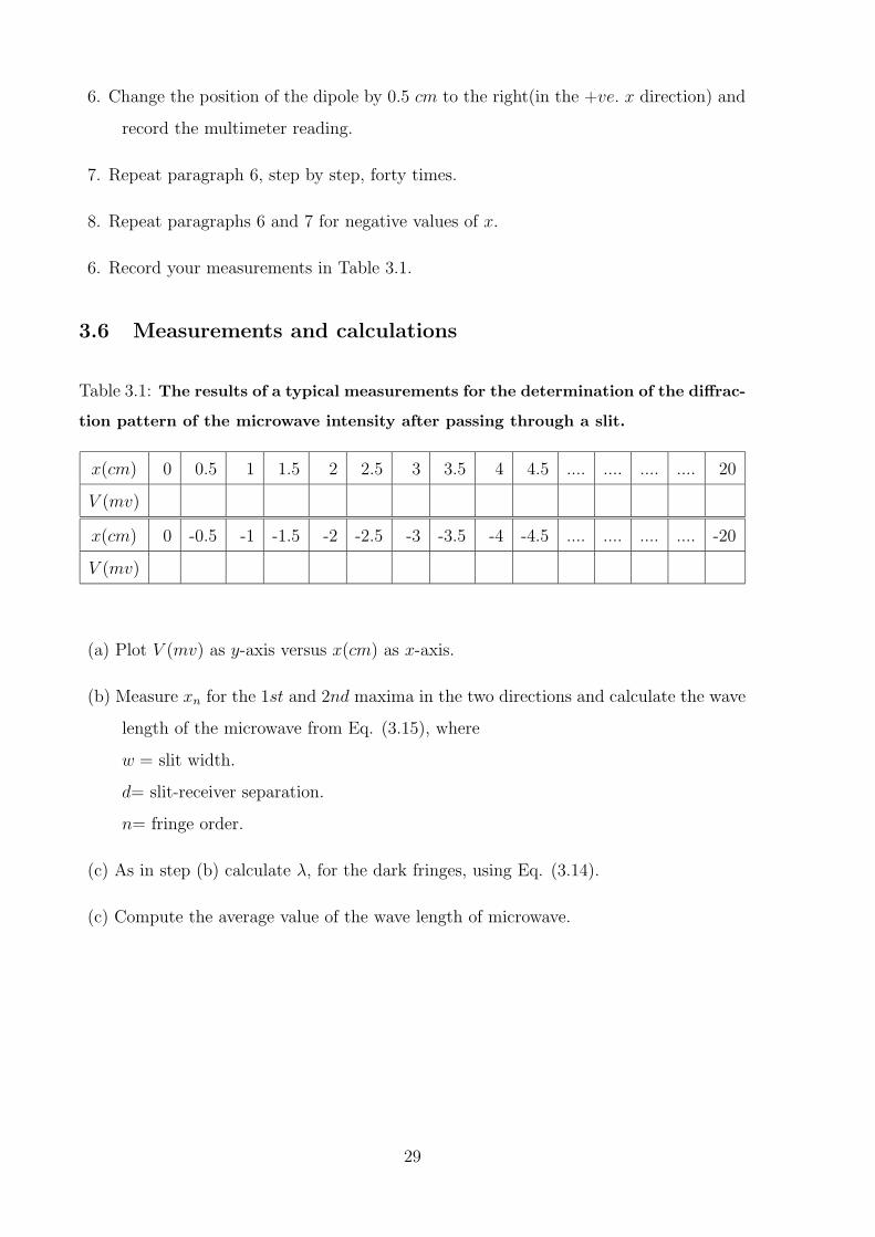
3.6 Measurements and calculations
Table 3.1: The results of a typical measurements for the determination of the diffrac-
tion pattern of the microwave intensity after passing through a slit.
x(cm) 0 0.5 1 1.5 2 2.5 3 3.5 4 4.5 .... .... .... .... 20
V (mv)
x(cm) 0 -0.5 -1 -1.5 -2 -2.5 -3 -3.5 -4 -4.5 .... .... .... .... -20
V (mv)
(a) Plot V (mv) as y-axis versus x(cm) as x-axis.
(b) Measure xn for the 1st and 2nd maxima in the two directions and calculate the wave
length of the microwave from Eq. (3.15), where
w = slit width.
d= slit-receiver separation.
n= fringe order.
(c) As in step (b) calculate λ, for the dark fringes, using Eq. (3.14).
(c) Compute the average value of the wave length of microwave.
29
4 Refraction Through Prism
4.1 Objective
1.To determine the refractive index of glass prism.
2.To determine the refractive index of various liquids in a hollow prism.
4.2 Principle and Task
The refractive indices of liquids and glass are determined by refraction of light through
the prism at minimum deviation.
4.3 Theory
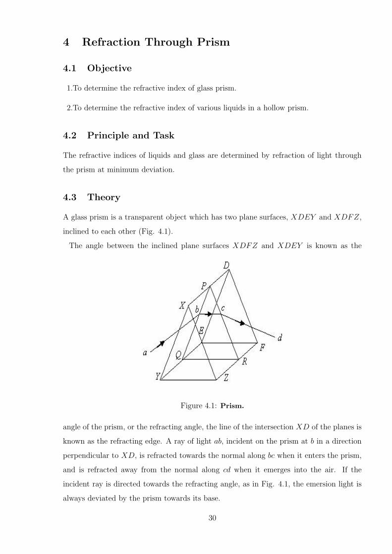
A glass prism is a transparent object which has two plane surfaces, XDEY and XDFZ,
inclined to each other (Fig. 4.1).
The angle between the inclined plane surfaces XDFZ and XDEY is known as the
Figure 4.1: Prism.
angle of the prism, or the refracting angle, the line of the intersection XD of the planes is
known as the refracting edge. A ray of light ab, incident on the prism at b in a direction
perpendicular to XD, is refracted towards the normal along bc when it enters the prism,
and is refracted away from the normal along cd when it emerges into the air. If the
incident ray is directed towards the refracting angle, as in Fig. 4.1, the emersion light is
always deviated by the prism towards its base.
30
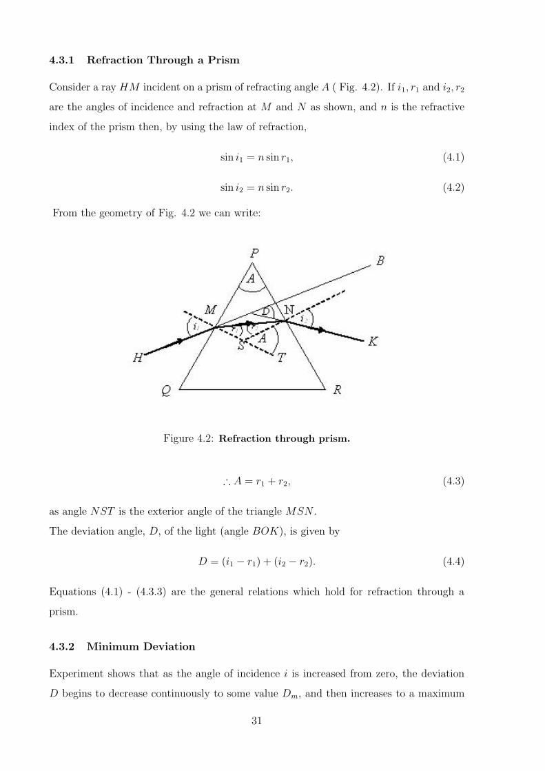
4.3.1 Refraction Through a Prism
Consider a ray HM incident on a prism of refracting angle A ( Fig. 4.2). If i1, r1 and i2, r2
are the angles of incidence and refraction at M and N as shown, and n is the refractive
index of the prism then, by using the law of refraction,
sin i1 = n sin r1, (4.1)
sin i2 = n sin r2. (4.2)
From the geometry of Fig. 4.2 we can write:
Figure 4.2: Refraction through prism.
∴ A = r1 + r2, (4.3)
as angle NST is the exterior angle of the triangle MSN .
The deviation angle, D, of the light (angle BOK), is given by
D = (i1 − r1) + (i2 − r2). (4.4)
Equations (4.1) - (4.3.3) are the general relations which hold for refraction through a
prism.
4.3.2 Minimum Deviation
Experiment shows that as the angle of incidence i is increased from zero, the deviation
D begins to decrease continuously to some value Dm, and then increases to a maximum
31
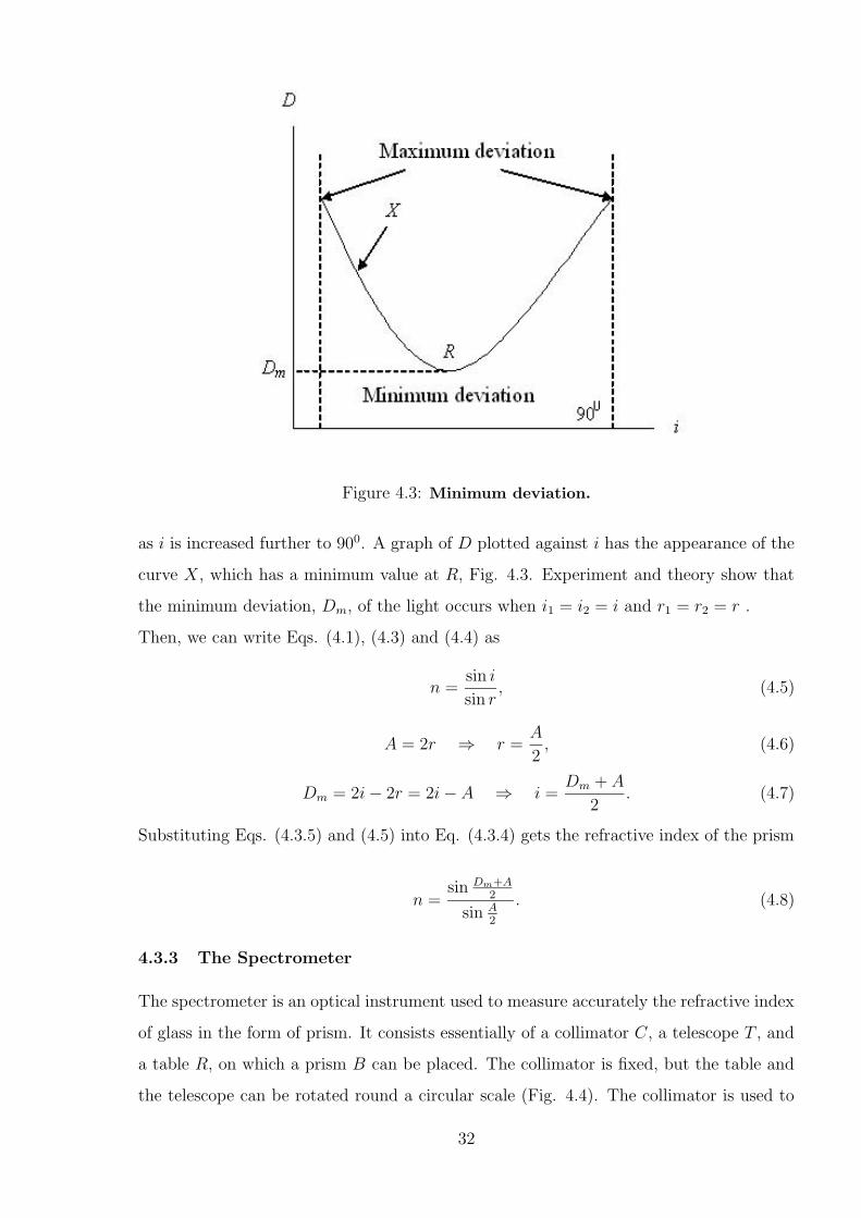
Figure 4.3: Minimum deviation.
as i is increased further to 900. A graph of D plotted against i has the appearance of the
curve X, which has a minimum value at R, Fig. 4.3. Experiment and theory show that
the minimum deviation, Dm, of the light occurs when i1 = i2 = i and r1 = r2 = r .
Then, we can write Eqs. (4.1), (4.3) and (4.4) as
n =sin i
sin r, (4.5)
A = 2r ⇒ r =A
2, (4.6)
Dm = 2i− 2r = 2i− A ⇒ i =Dm + A
2. (4.7)
Substituting Eqs. (4.3.5) and (4.5) into Eq. (4.3.4) gets the refractive index of the prism
n =sin Dm+A
2
sin A2
. (4.8)
4.3.3 The Spectrometer
The spectrometer is an optical instrument used to measure accurately the refractive index
of glass in the form of prism. It consists essentially of a collimator C, a telescope T , and
a table R, on which a prism B can be placed. The collimator is fixed, but the table and
the telescope can be rotated round a circular scale (Fig. 4.4). The collimator is used to
32
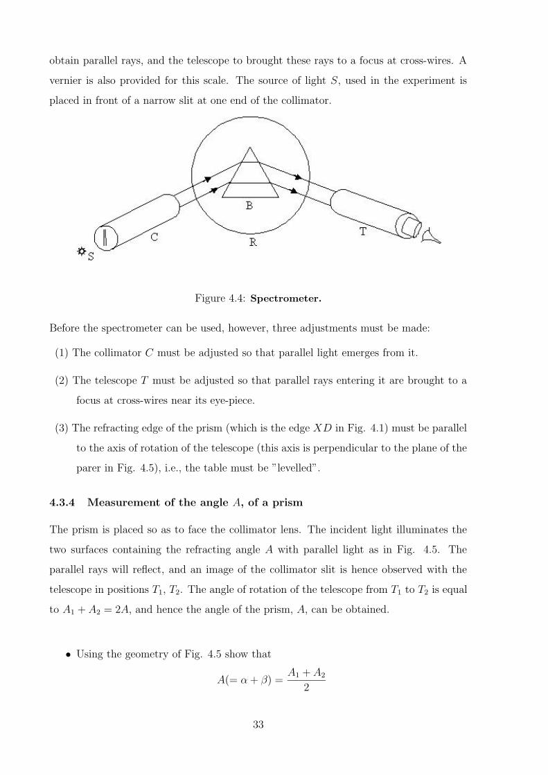
obtain parallel rays, and the telescope to brought these rays to a focus at cross-wires. A
vernier is also provided for this scale. The source of light S, used in the experiment is
placed in front of a narrow slit at one end of the collimator.
Figure 4.4: Spectrometer.
Before the spectrometer can be used, however, three adjustments must be made:
(1) The collimator C must be adjusted so that parallel light emerges from it.
(2) The telescope T must be adjusted so that parallel rays entering it are brought to a
focus at cross-wires near its eye-piece.
(3) The refracting edge of the prism (which is the edge XD in Fig. 4.1) must be parallel
to the axis of rotation of the telescope (this axis is perpendicular to the plane of the
parer in Fig. 4.5), i.e., the table must be ”levelled”.
4.3.4 Measurement of the angle A, of a prism
The prism is placed so as to face the collimator lens. The incident light illuminates the
two surfaces containing the refracting angle A with parallel light as in Fig. 4.5. The
parallel rays will reflect, and an image of the collimator slit is hence observed with the
telescope in positions T1, T2. The angle of rotation of the telescope from T1 to T2 is equal
to A1 + A2 = 2A, and hence the angle of the prism, A, can be obtained.
• Using the geometry of Fig. 4.5 show that
A(= α+ β) =A1 + A2
2
33
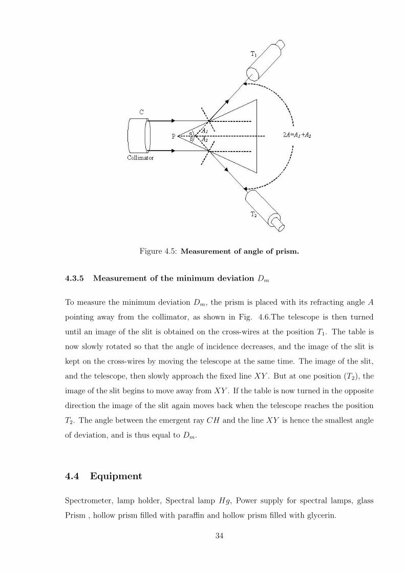
Figure 4.5: Measurement of angle of prism.
4.3.5 Measurement of the minimum deviation Dm
To measure the minimum deviation Dm, the prism is placed with its refracting angle A
pointing away from the collimator, as shown in Fig. 4.6.The telescope is then turned
until an image of the slit is obtained on the cross-wires at the position T1. The table is
now slowly rotated so that the angle of incidence decreases, and the image of the slit is
kept on the cross-wires by moving the telescope at the same time. The image of the slit,
and the telescope, then slowly approach the fixed line XY . But at one position (T2), the
image of the slit begins to move away from XY . If the table is now turned in the opposite
direction the image of the slit again moves back when the telescope reaches the position
T2. The angle between the emergent ray CH and the line XY is hence the smallest angle
of deviation, and is thus equal to Dm.
4.4 Equipment
Spectrometer, lamp holder, Spectral lamp Hg, Power supply for spectral lamps, glass
Prism , hollow prism filled with paraffin and hollow prism filled with glycerin.
34
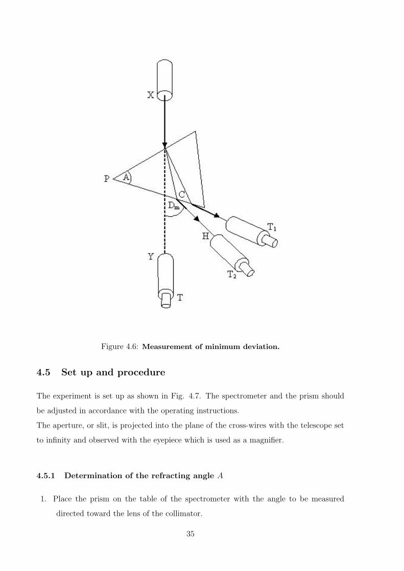
Figure 4.6: Measurement of minimum deviation.
4.5 Set up and procedure
The experiment is set up as shown in Fig. 4.7. The spectrometer and the prism should
be adjusted in accordance with the operating instructions.
The aperture, or slit, is projected into the plane of the cross-wires with the telescope set
to infinity and observed with the eyepiece which is used as a magnifier.
4.5.1 Determination of the refracting angle A
1. Place the prism on the table of the spectrometer with the angle to be measured
directed toward the lens of the collimator.
35
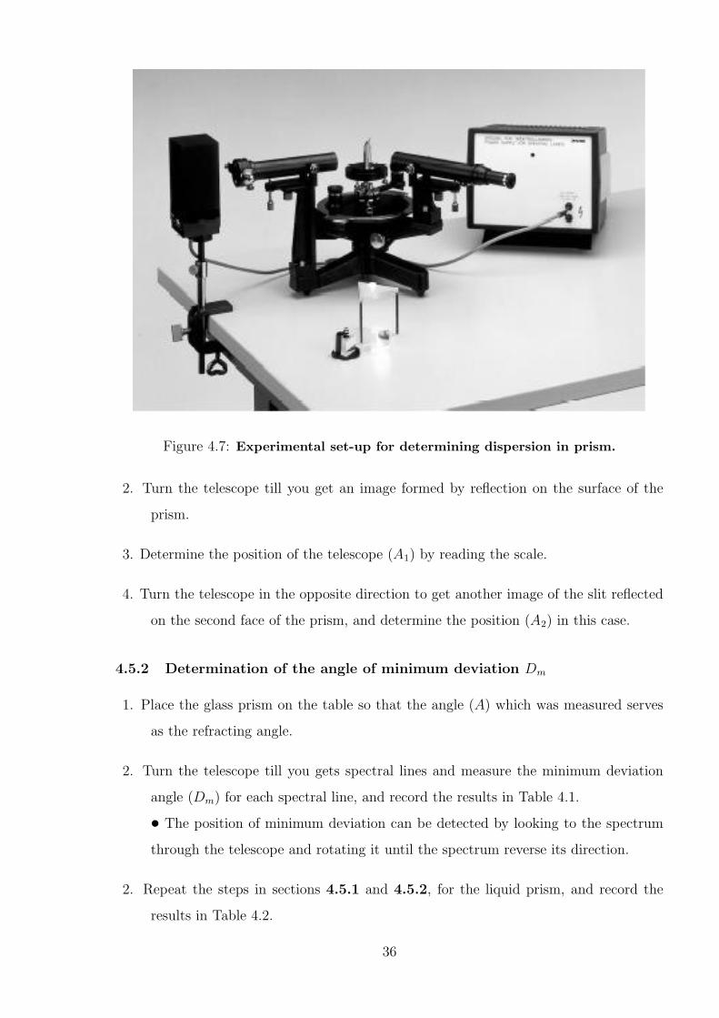
Figure 4.7: Experimental set-up for determining dispersion in prism.
2. Turn the telescope till you get an image formed by reflection on the surface of the
prism.
3. Determine the position of the telescope (A1) by reading the scale.
4. Turn the telescope in the opposite direction to get another image of the slit reflected
on the second face of the prism, and determine the position (A2) in this case.
4.5.2 Determination of the angle of minimum deviation Dm
1. Place the glass prism on the table so that the angle (A) which was measured serves
as the refracting angle.
2. Turn the telescope till you gets spectral lines and measure the minimum deviation
angle (Dm) for each spectral line, and record the results in Table 4.1.
• The position of minimum deviation can be detected by looking to the spectrum
through the telescope and rotating it until the spectrum reverse its direction.
2. Repeat the steps in sections 4.5.1 and 4.5.2, for the liquid prism, and record the
results in Table 4.2.
36
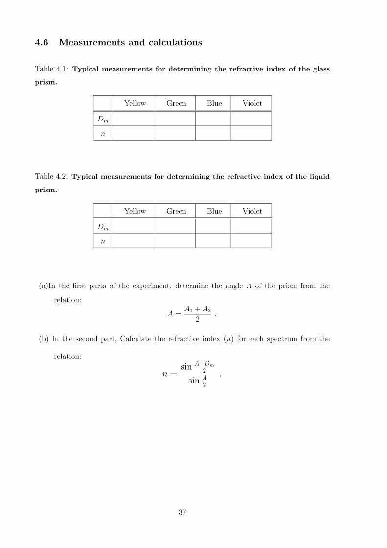
4.6 Measurements and calculations
Table 4.1: Typical measurements for determining the refractive index of the glass
prism.
Yellow Green Blue Violet
Dm
n
Table 4.2: Typical measurements for determining the refractive index of the liquid
prism.
Yellow Green Blue Violet
Dm
n
(a)In the first parts of the experiment, determine the angle A of the prism from the
relation:
A =A1 + A2
2.
(b) In the second part, Calculate the refractive index (n) for each spectrum from the
relation:
n =sin A+Dm
2
sin A2
.
37
5 Polarimetry
5.1 Objective
To determine the specific rotation of a sugar by measuring the rotation of various solutions
of known concentration.
5.2 Principle and Task
The rotation of the plane of polarization through a sugar solution measured with a po-
larimeter and the specific rotation of the sugar determined.
5.3 Theory
The experiments on interference and diffraction have shown that light is a form of wave
motion. These effects do not tell us about the type of wave motion i.e., whether the
light waves are longitudinal or transverse, or whether the vibrations are linear, circular
or torsional. The phenomenon of polarization has helped to establish beyond doubt that
light waves are transverse waves.
5.3.1 Polarization of light waves
Let light from a source S fall on a tourmaline crystal A which is cut parallel to its axis
(Fig. 5.1). On rotating the crystal A, no remarkable change is noticed. Now place the
crystal B parallel to A.
1. Rotate the crystals together so that their axes are always parallel. No change is
observed in the light coming out of B (Fig. 5.1 a).
2. Keep the crystal A fixed and rotate the crystal B. The light transmitted through B
becomes dimmer and dimmer. When B is at right angles to A, no light emerges out
of B (Fig. 5.1 b).
If the crystal B is further rotated, the intensity of light coming out of it gradually in-
creases and is maximum again when the two crystals are parallel.
This experiment shows conclusively that light is not propagated as longitudinal or com-
pressional waves. If we consider the propagation of light as a longitudinal wave motion
38
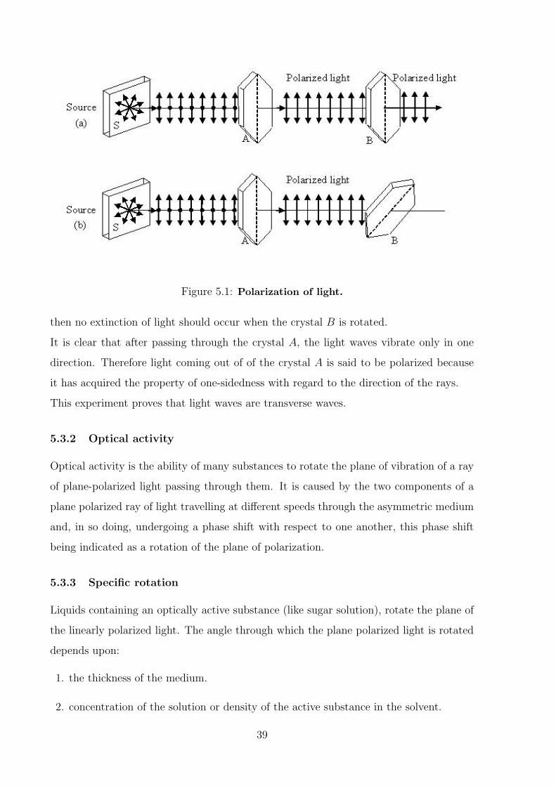
Figure 5.1: Polarization of light.
then no extinction of light should occur when the crystal B is rotated.
It is clear that after passing through the crystal A, the light waves vibrate only in one
direction. Therefore light coming out of of the crystal A is said to be polarized because
it has acquired the property of one-sidedness with regard to the direction of the rays.
This experiment proves that light waves are transverse waves.
5.3.2 Optical activity
Optical activity is the ability of many substances to rotate the plane of vibration of a ray
of plane-polarized light passing through them. It is caused by the two components of a
plane polarized ray of light travelling at different speeds through the asymmetric medium
and, in so doing, undergoing a phase shift with respect to one another, this phase shift
being indicated as a rotation of the plane of polarization.
5.3.3 Specific rotation
Liquids containing an optically active substance (like sugar solution), rotate the plane of
the linearly polarized light. The angle through which the plane polarized light is rotated
depends upon:
1. the thickness of the medium.
2. concentration of the solution or density of the active substance in the solvent.
39
3. wave length of light.
4. temperature.
The specific rotation (rotatory power) is defined as the rotation produced by a decimeter
(10cm) long column of the liquid containing 1gm of the active substance in one cc (cm3)
of solution. Therefore,
Stλ =10θ
lc(5.1)
where Stλ represents the specific rotation at temperature t oC for a wave length λ,θ is the
angle of rotation, l is the length of the solution in cm through which the plane polarized
light passes and c is the concentration of the active substance ingm/cm3 in the solution.
The angle through which the plane of polarization is rotated by the optically active
substance is determined with the help of a polarimeter.
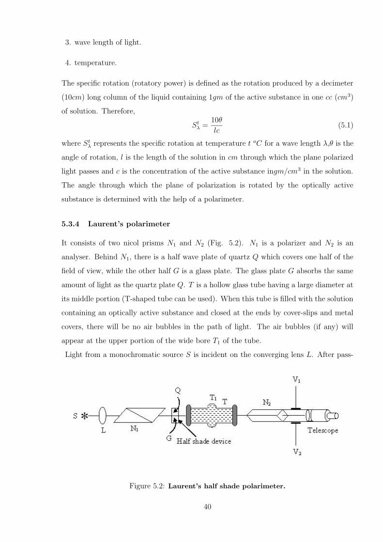
5.3.4 Laurent’s polarimeter
It consists of two nicol prisms N1 and N2 (Fig. 5.2). N1 is a polarizer and N2 is an
analyser. Behind N1, there is a half wave plate of quartz Q which covers one half of the
field of view, while the other half G is a glass plate. The glass plate G absorbs the same
amount of light as the quartz plate Q. T is a hollow glass tube having a large diameter at
its middle portion (T-shaped tube can be used). When this tube is filled with the solution
containing an optically active substance and closed at the ends by cover-slips and metal
covers, there will be no air bubbles in the path of light. The air bubbles (if any) will
appear at the upper portion of the wide bore T1 of the tube.
Light from a monochromatic source S is incident on the converging lens L. After pass-
Figure 5.2: Laurent’s half shade polarimeter.
40
ing through N1, the beam is plane polarized. One half of the beam passes through the
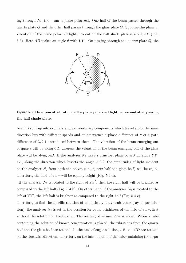
quartz plate Q and the other half passes through the glass plate G. Suppose the plane of
vibration of the plane polarized light incident on the half shade plate is along AB (Fig.
5.3). Here AB makes an angle θ with Y Y′
. On passing through the quartz plate Q, the
Figure 5.3: Direction of vibration of the plane polarized light before and after passing
the half shade plate.
beam is split up into ordinary and extraordinary components which travel along the same
direction but with different speeds and on emergence a phase difference of π or a path
difference of λ/2 is introduced between them. The vibration of the beam emerging out
of quartz will be along CD whereas the vibration of the beam emerging out of the glass
plate will be along AB. If the analyser N2 has its principal plane or section along Y Y′
i.e., along the direction which bisects the angle AOC, the amplitudes of light incident
on the analyser N2 from both the halves (i.e., quartz half and glass half) will be equal.
Therefore, the field of view will be equally bright (Fig. 5.4 a).
If the analyser N2 is rotated to the right of Y Y′
, then the right half will be brighter as
compared to the left half (Fig. 5.4 b). On other hand, if the analyser N2 is rotated to the
left of Y Y′
, the left half is brighter as compared to the right half (Fig. 5.4 c).
Therefore, to find the specific rotation of an optically active substance (say, sugar solu-
tion), the analyser N2 is set in the position for equal brightness of the field of view, first
without the solution on the tube T . The reading of vernier V1V2 is noted. When a tube
containing the solution of known concentration is placed, the vibrations from the quartz
half and the glass half are rotated. In the case of sugar solution, AB and CD are rotated
on the clockwise direction. Therefore, on the introduction of the tube containing the sugar
41
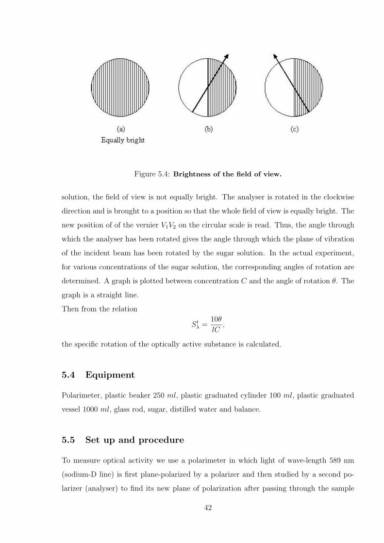
Figure 5.4: Brightness of the field of view.
solution, the field of view is not equally bright. The analyser is rotated in the clockwise
direction and is brought to a position so that the whole field of view is equally bright. The
new position of of the vernier V1V2 on the circular scale is read. Thus, the angle through
which the analyser has been rotated gives the angle through which the plane of vibration
of the incident beam has been rotated by the sugar solution. In the actual experiment,
for various concentrations of the sugar solution, the corresponding angles of rotation are
determined. A graph is plotted between concentration C and the angle of rotation θ. The
graph is a straight line.
Then from the relation
Stλ =10θ
lC,
the specific rotation of the optically active substance is calculated.
5.4 Equipment
Polarimeter, plastic beaker 250 ml, plastic graduated cylinder 100 ml, plastic graduated
vessel 1000 ml, glass rod, sugar, distilled water and balance.
5.5 Set up and procedure
To measure optical activity we use a polarimeter in which light of wave-length 589 nm
(sodium-D line) is first plane-polarized by a polarizer and then studied by a second po-
larizer (analyser) to find its new plane of polarization after passing through the sample
42
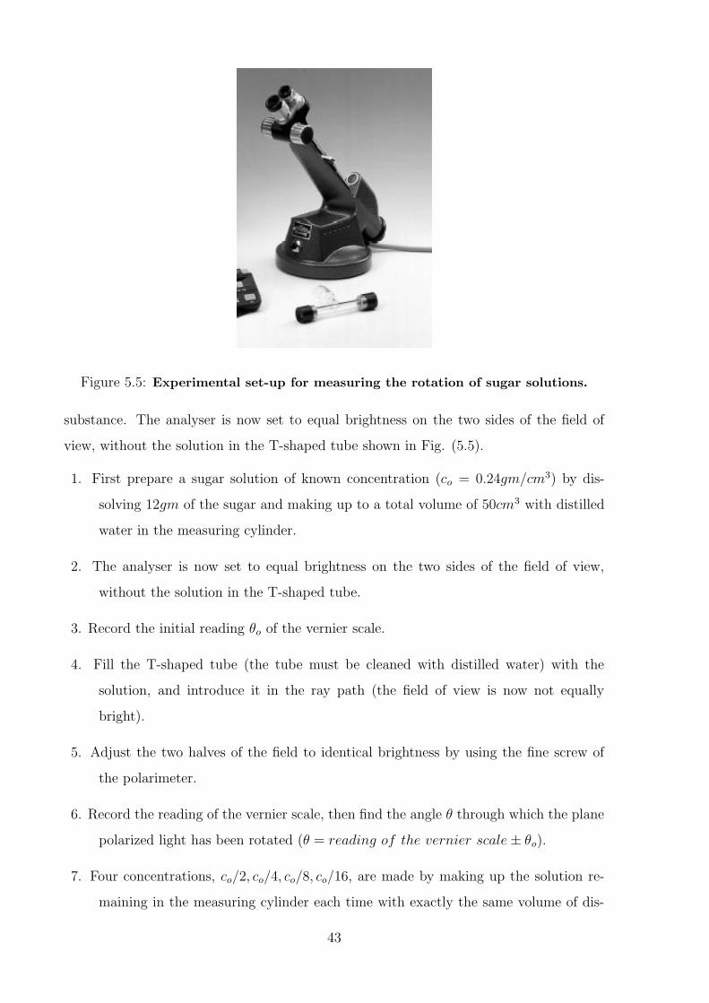
Figure 5.5: Experimental set-up for measuring the rotation of sugar solutions.
substance. The analyser is now set to equal brightness on the two sides of the field of
view, without the solution in the T-shaped tube shown in Fig. (5.5).
1. First prepare a sugar solution of known concentration (co = 0.24gm/cm3) by dis-
solving 12gm of the sugar and making up to a total volume of 50cm3 with distilled
water in the measuring cylinder.
2. The analyser is now set to equal brightness on the two sides of the field of view,
without the solution in the T-shaped tube.
3. Record the initial reading θo of the vernier scale.
4. Fill the T-shaped tube (the tube must be cleaned with distilled water) with the
solution, and introduce it in the ray path (the field of view is now not equally
bright).
5. Adjust the two halves of the field to identical brightness by using the fine screw of
the polarimeter.
6. Record the reading of the vernier scale, then find the angle θ through which the plane
polarized light has been rotated (θ = reading of the vernier scale± θo).
7. Four concentrations, co/2, co/4, co/8, co/16, are made by making up the solution re-
maining in the measuring cylinder each time with exactly the same volume of dis-
43
tilled water.
• Remark
Don’t prepare these solutions until you finish the measurement of the previous one,
that is, prepare co/2 then proceed to step 8 and so on.
8. Repeat paragraphes 4-6 for each of the solutions prepared in step 7, and record the
results in Table 5.1.
5.6 Measurements and calculations
Table 5.1: The results of a typical measurements for the determination of the specific
rotation of the cane sugar.
c (gm/cm3) 0.24 0.12 0.06 0.03 0.015
θo
A graph is plotted between concentration c as x-axis and the angle of rotation θ as
y-axis (Fig. 5.6).
From the relation
Stλ =10θ
lc,
the specific rotation of sugar can be calculated.
Stλ =θ
c= slope,
(related to a column length of 10 cm)
44
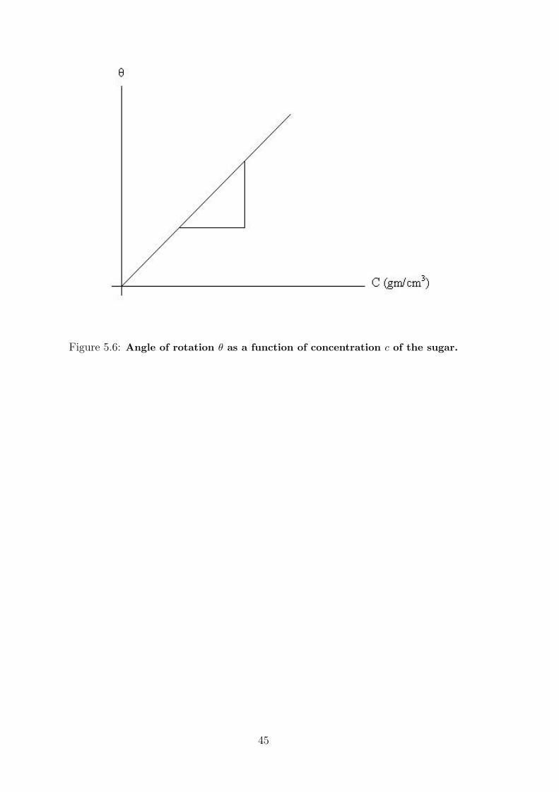
Figure 5.6: Angle of rotation θ as a function of concentration c of the sugar.
45
6 Measuring the Velocity of Light
6.1 Objective
1. To determine the velocity of light in air.
2. To determine the velocity of light in water and synthetic resin and to calculate the
refractive indices.
6.2 Principle and Task
The intensity of the light is modulated and the phase relationship of the transmitter and
receiver signal compared. The velocity of light is calculated from the relationship between
the changes in the phase and the light path.
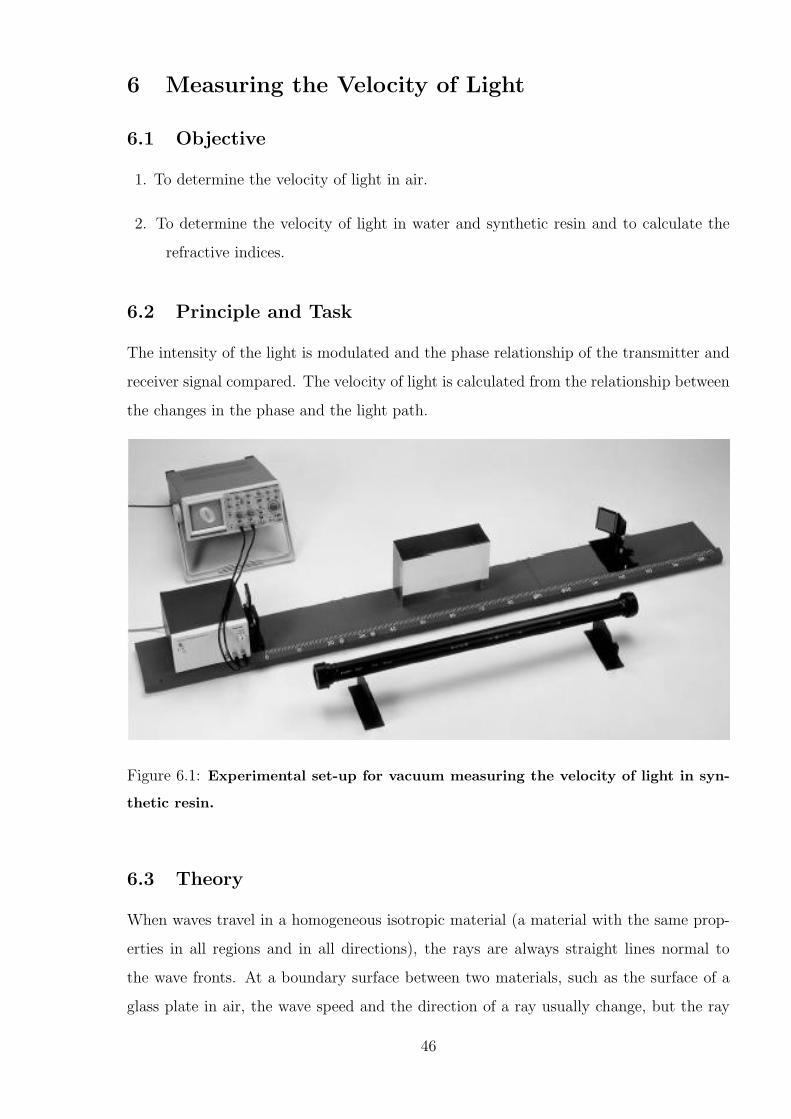
Figure 6.1: Experimental set-up for vacuum measuring the velocity of light in syn-
thetic resin.
6.3 Theory
When waves travel in a homogeneous isotropic material (a material with the same prop-
erties in all regions and in all directions), the rays are always straight lines normal to
the wave fronts. At a boundary surface between two materials, such as the surface of a
glass plate in air, the wave speed and the direction of a ray usually change, but the ray
46
segments in the air and in the glass are straight lines. The ratio of the speed of light in
air ca to the speed of light in a medium cm is called the refractive index n of the medium.
n =cacm
. (6.1)
6.3.1 Composition of two simple harmonic motions acting at right angles
Let
x = a sin(ωt+ α) (6.2)
and
y = b sin(ωt) (6.3)
represent the displacements of a particle along the x− and y−axes due to the influence
of two simple harmonic vibrations acting simultaneously on a particle in perpendicular
directions. Here, the two vibrations are of the same time period but are of different
amplitudes and different phase angles.
From (6.3.1),
sinωt =y
b, (6.4)
∴ cosωt =
√
1−y2
b2. (6.5)
From Eq. (6.3.1),x
a= (sinωt cosα + cosωt sinα) . (6.6)
Substituting the value of sinωt and cosωt in Eq. (6.6)
x
a=
(
y
b· cosα+
√
1−y2
b2· sinα
)
, (6.7)
orx
a−y
b· cosα =
√
1−y2
b2· sinα. (6.8)
Squaring Eq. (6.8)
x2
a2+y2
b2· cos2 α−
2xy
ab· cosα =
(
1−y2
b2
)
sin2 α, (6.9)
orx2
a2+y2
b2(
sin2 α + cos2 α)
−2xy
ab· cosα = sin2 α, (6.10)
∴x2
a2+y2
b2−
2xy
ab· cosα = sin2 α. (6.11)
47
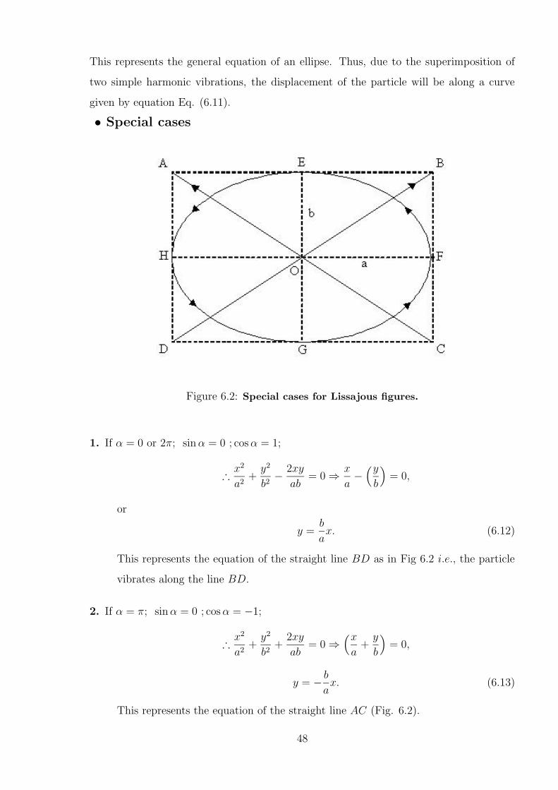
This represents the general equation of an ellipse. Thus, due to the superimposition of
two simple harmonic vibrations, the displacement of the particle will be along a curve
given by equation Eq. (6.11).
• Special cases
Figure 6.2: Special cases for Lissajous figures.
1. If α = 0 or 2π; sinα = 0 ; cosα = 1;
∴x2
a2+y2
b2−
2xy
ab= 0⇒
x
a−(y
b
)
= 0,
or
y =b
ax. (6.12)
This represents the equation of the straight line BD as in Fig 6.2 i.e., the particle
vibrates along the line BD.
2. If α = π; sinα = 0 ; cosα = −1;
∴x2
a2+y2
b2+
2xy
ab= 0⇒
(x
a+y
b
)
= 0,
y = −b
ax. (6.13)
This represents the equation of the straight line AC (Fig. 6.2).
48
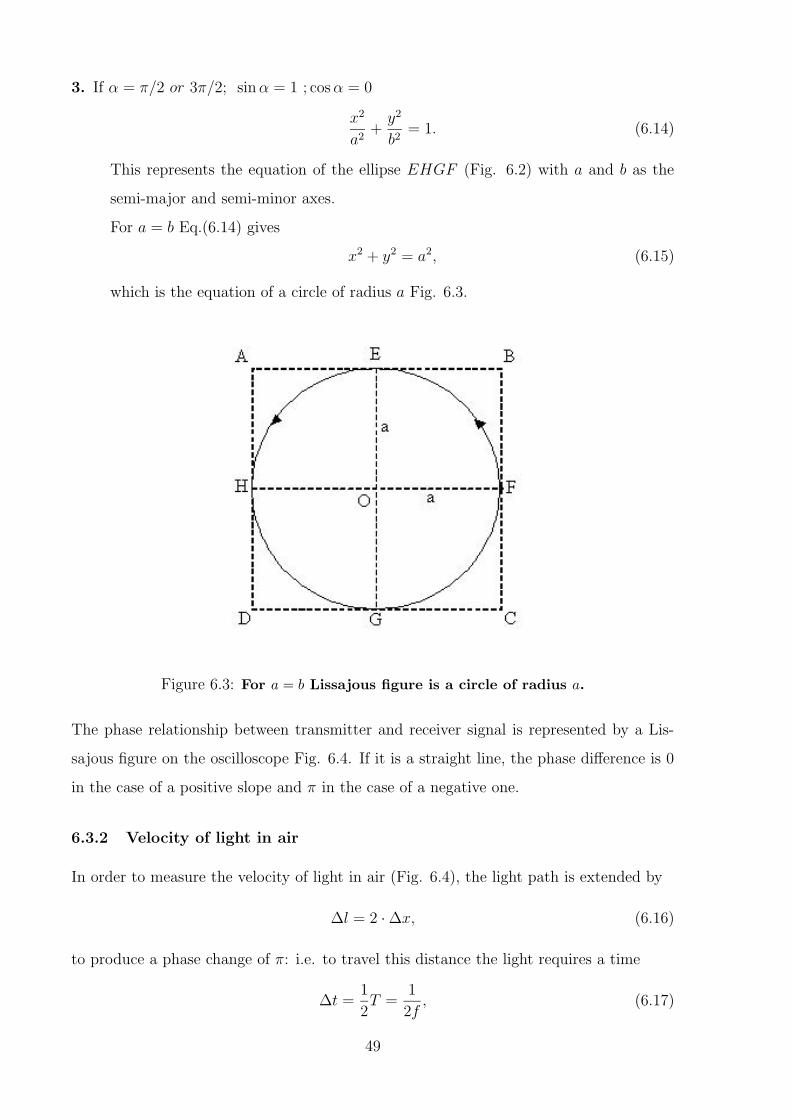
3. If α = π/2 or 3π/2; sinα = 1 ; cosα = 0
x2
a2+y2
b2= 1. (6.14)
This represents the equation of the ellipse EHGF (Fig. 6.2) with a and b as the
semi-major and semi-minor axes.
For a = b Eq.(6.14) gives
x2 + y2 = a2, (6.15)
which is the equation of a circle of radius a Fig. 6.3.
Figure 6.3: For a = b Lissajous figure is a circle of radius a.
The phase relationship between transmitter and receiver signal is represented by a Lis-
sajous figure on the oscilloscope Fig. 6.4. If it is a straight line, the phase difference is 0
in the case of a positive slope and π in the case of a negative one.
6.3.2 Velocity of light in air
In order to measure the velocity of light in air (Fig. 6.4), the light path is extended by
∆l = 2 ·∆x, (6.16)
to produce a phase change of π: i.e. to travel this distance the light requires a time
∆t =1
2T =
1
2f, (6.17)
49
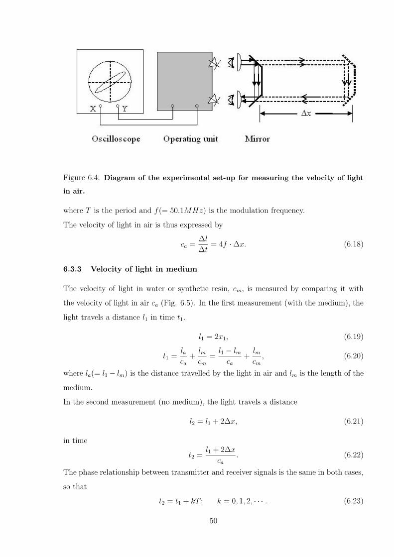
Figure 6.4: Diagram of the experimental set-up for measuring the velocity of light
in air.
where T is the period and f(= 50.1MHz) is the modulation frequency.
The velocity of light in air is thus expressed by
ca =∆l
∆t= 4f ·∆x. (6.18)
6.3.3 Velocity of light in medium
The velocity of light in water or synthetic resin, cm, is measured by comparing it with
the velocity of light in air ca (Fig. 6.5). In the first measurement (with the medium), the
light travels a distance l1 in time t1.
l1 = 2x1, (6.19)
t1 =laca
+lmcm
=l1 − lmca
+lmcm
, (6.20)
where la(= l1 − lm) is the distance travelled by the light in air and lm is the length of the
medium.
In the second measurement (no medium), the light travels a distance
l2 = l1 + 2∆x, (6.21)
in time
t2 =l1 + 2∆x
ca. (6.22)
The phase relationship between transmitter and receiver signals is the same in both cases,
so that
t2 = t1 + kT ; k = 0, 1, 2, · · · . (6.23)
50
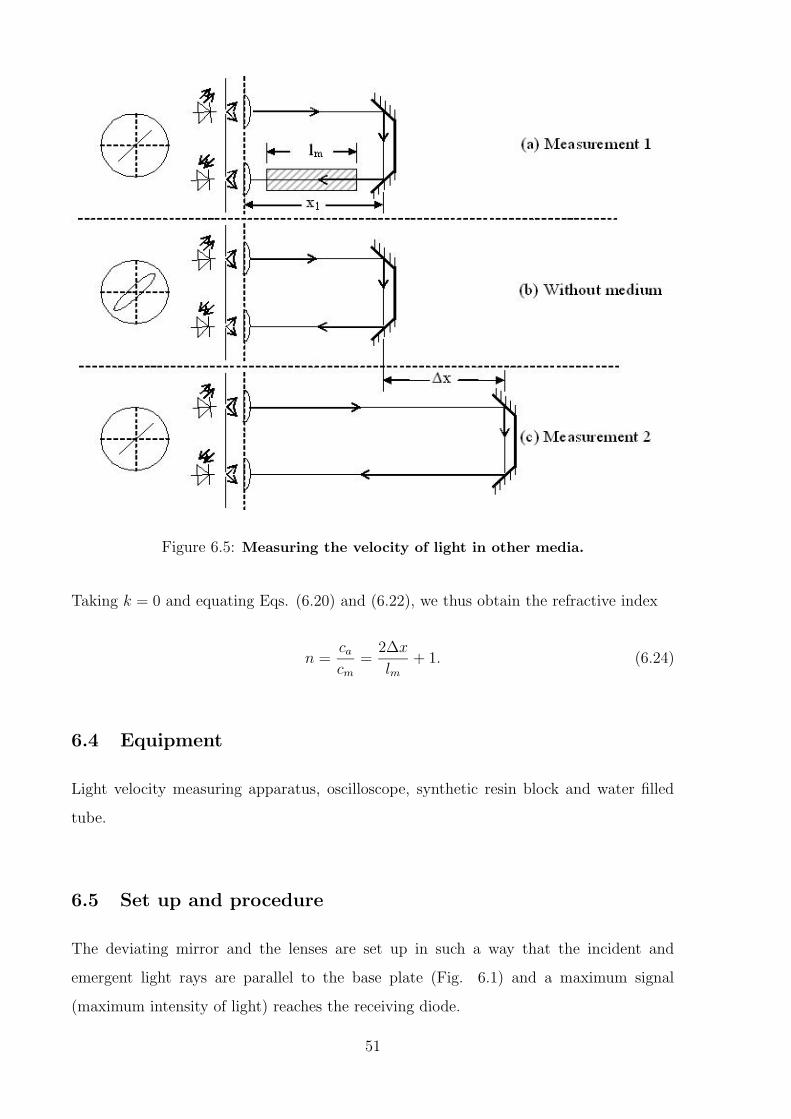
Figure 6.5: Measuring the velocity of light in other media.
Taking k = 0 and equating Eqs. (6.20) and (6.22), we thus obtain the refractive index
n =cacm
=2∆x
lm+ 1. (6.24)
6.4 Equipment
Light velocity measuring apparatus, oscilloscope, synthetic resin block and water filled
tube.
6.5 Set up and procedure
The deviating mirror and the lenses are set up in such a way that the incident and
emergent light rays are parallel to the base plate (Fig. 6.1) and a maximum signal
(maximum intensity of light) reaches the receiving diode.
51
6.5.1 Adjustment of the apparatus
1. Place the two lenses in front of the transmitter and the receiver (the flat surface must
be towards the operating unit).
2. Placed the mirror as far to the operating unit as possible.
3. Adjust the position of the lens, which is in front of the transmitter, until a spot of
light is appear on the surface of the mirror (you can use a white paper in the path
of the light ray in order to see this spot of light).
4. The light beam will reflect to incident on the second part of the mirror, and the spot
of light will appear on its surface (use the white paper to see the spot).
5. Adjust the screws, fitted on the mirror, so that the beam of light is incident on the
convex surface of the lens, which is in front of the receiver.
6. Adjust the position of this lens until the light is concentrated on the receiving diode.
6.5.2 Measuring the velocity of light in air
1. The mirror is now placed as close to the operating unit as possible (zero point on the
scale) and a Lissajous figure appears on the oscilloscope.
2. Using the ’phase’ knob on the operating unit, transform the Lissajous figure into a
straight line.
3. The mirror is then slide along the graduated scale until the phase has changed by π,
i.e. until a straight line sloping in the opposite direction is obtained.
4. The mirror displacement ∆x is measured; the measurement should be repeated several
times (four times at least).
5. Record the results in Table 6.1.
6.Using Eq. (6.18) calculate the velocity of light in air.
52
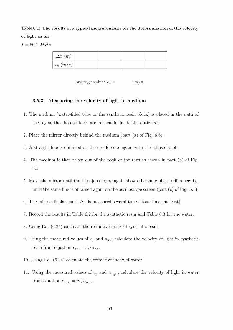
Table 6.1: The results of a typical measurements for the determination of the velocity
of light in air.
f = 50.1 MHz
∆x (m)
ca (m/s)
average value: ca = cm/s
6.5.3 Measuring the velocity of light in medium
1. The medium (water-filled tube or the synthetic resin block) is placed in the path of
the ray so that its end faces are perpendicular to the optic axis.
2. Place the mirror directly behind the medium (part (a) of Fig. 6.5).
3. A straight line is obtained on the oscilloscope again with the ’phase’ knob.
4. The medium is then taken out of the path of the rays as shown in part (b) of Fig.
6.5.
5. Move the mirror until the Lissajous figure again shows the same phase difference; i.e,
until the same line is obtained again on the oscilloscope screen (part (c) of Fig. 6.5).
6. The mirror displacement ∆x is measured several times (four times at least).
7. Record the results in Table 6.2 for the synthetic resin and Table 6.3 for the water.
8. Using Eq. (6.24) calculate the refractive index of synthetic resin.
9. Using the measured values of ca and ns.r, calculate the velocity of light in synthetic
resin from equation cs.r = ca/ns.r.
10. Using Eq. (6.24) calculate the refractive index of water.
11. Using the measured values of ca and nH2O
, calculate the velocity of light in water
from equation cH2O
= ca/nH2O.
53
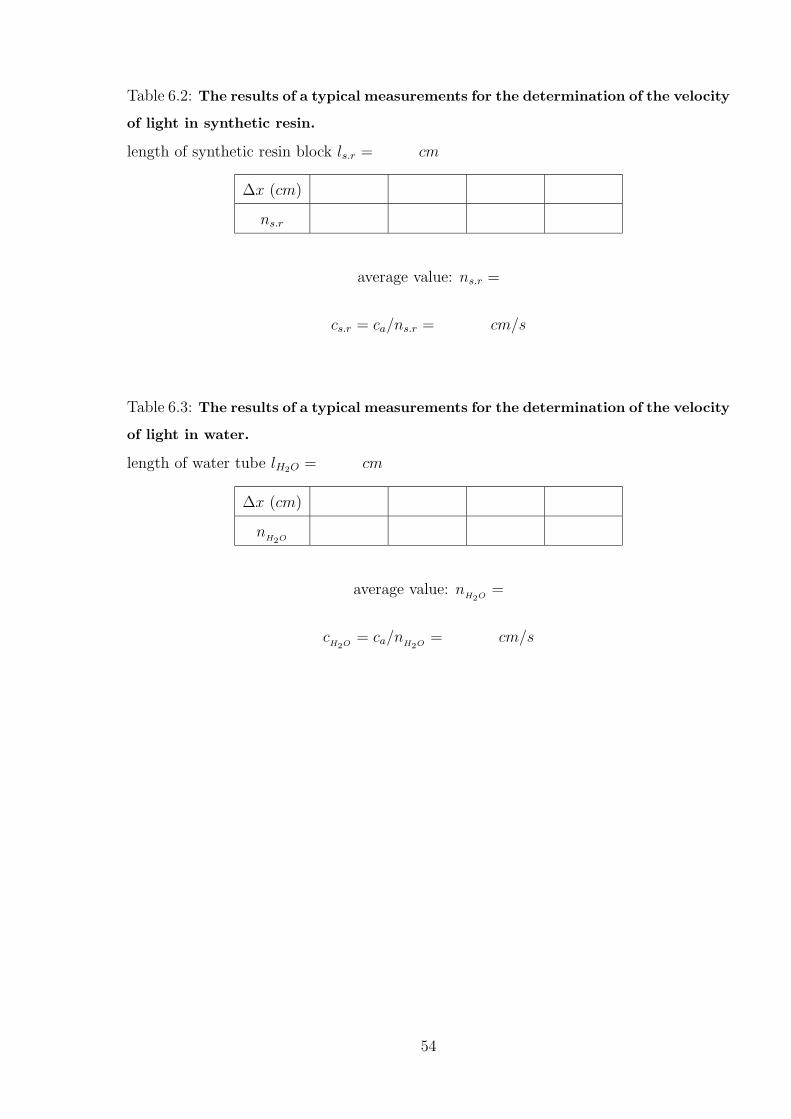
Table 6.2: The results of a typical measurements for the determination of the velocity
of light in synthetic resin.
length of synthetic resin block ls.r = cm
∆x (cm)
ns.r
average value: ns.r =
cs.r = ca/ns.r = cm/s
Table 6.3: The results of a typical measurements for the determination of the velocity
of light in water.
length of water tube lH2O = cm
∆x (cm)
nH2O
average value: nH2O
=
cH2O
= ca/nH2O= cm/s
54
7 Newton’s Rings
7.1 Objective
To determine the wavelengths for a given radius of curvature of the lens of Newton’s rings
apparatus.
7.2 Principle and Task
In a Newton’s rings apparatus, monochromatic light interferes in the thin film of air
between the slightly convex lens and a plane glass plate. The wavelengths are determined
from the radii of the interference rings.
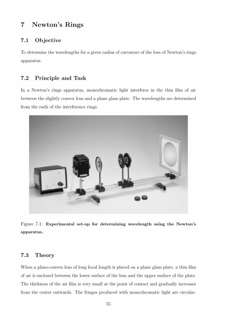
Figure 7.1: Experimental set-up for determining wavelength using the Newton’s
apparatus.
7.3 Theory
When a plano-convex lens of long focal length is placed on a plane glass plate, a thin film
of air is enclosed between the lower surface of the lens and the upper surface of the plate.
The thickness of the air film is very small at the point of contact and gradually increases
from the center outwards. The fringes produced with monochromatic light are circular.
55
The fringes are concentric circles, uniform in thickness and with the point of contact as
the center. When viewed with white light, the fringes are colored. With monochromatic
light, bright and dark circular fringes are produced in the air film.
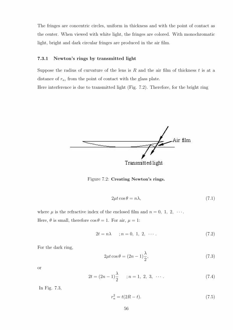
7.3.1 Newton’s rings by transmitted light
Suppose the radius of curvature of the lens is R and the air film of thickness t is at a
distance of rn, from the point of contact with the glass plate.
Here interference is due to transmitted light (Fig. 7.2). Therefore, for the bright ring
Figure 7.2: Creating Newton’s rings.
2µt cos θ = nλ, (7.1)
where µ is the refractive index of the enclosed film and n = 0, 1, 2, · · · .
Here, θ is small, therefore cos θ = 1. For air, µ = 1:
2t = nλ ;n = 0, 1, 2, · · · . (7.2)
For the dark ring,
2µt cos θ = (2n− 1)λ
2, (7.3)
or
2t = (2n− 1)λ
2;n = 1, 2, 3, · · · . (7.4)
In Fig. 7.3,
r2n = t(2R− t). (7.5)
56
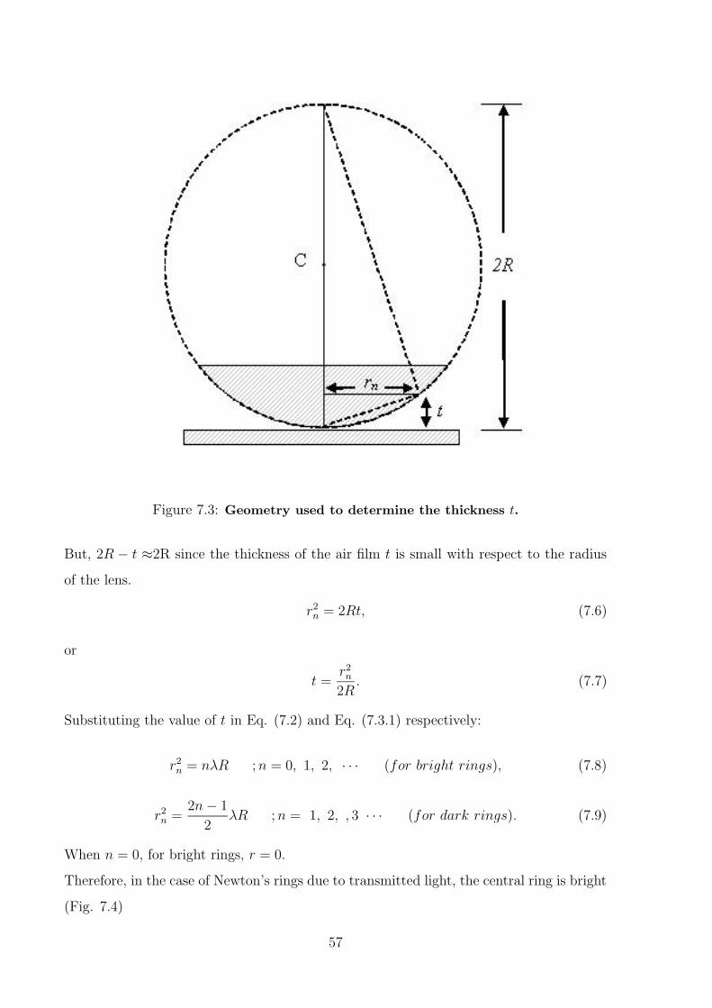
Figure 7.3: Geometry used to determine the thickness t.
But, 2R − t ≈2R since the thickness of the air film t is small with respect to the radius
of the lens.
r2n = 2Rt, (7.6)
or
t =r2n
2R. (7.7)
Substituting the value of t in Eq. (7.2) and Eq. (7.3.1) respectively:
r2n = nλR ;n = 0, 1, 2, · · · (for bright rings), (7.8)
r2n =
2n− 1
2λR ;n = 1, 2, , 3 · · · (for dark rings). (7.9)
When n = 0, for bright rings, r = 0.
Therefore, in the case of Newton’s rings due to transmitted light, the central ring is bright
(Fig. 7.4)
57
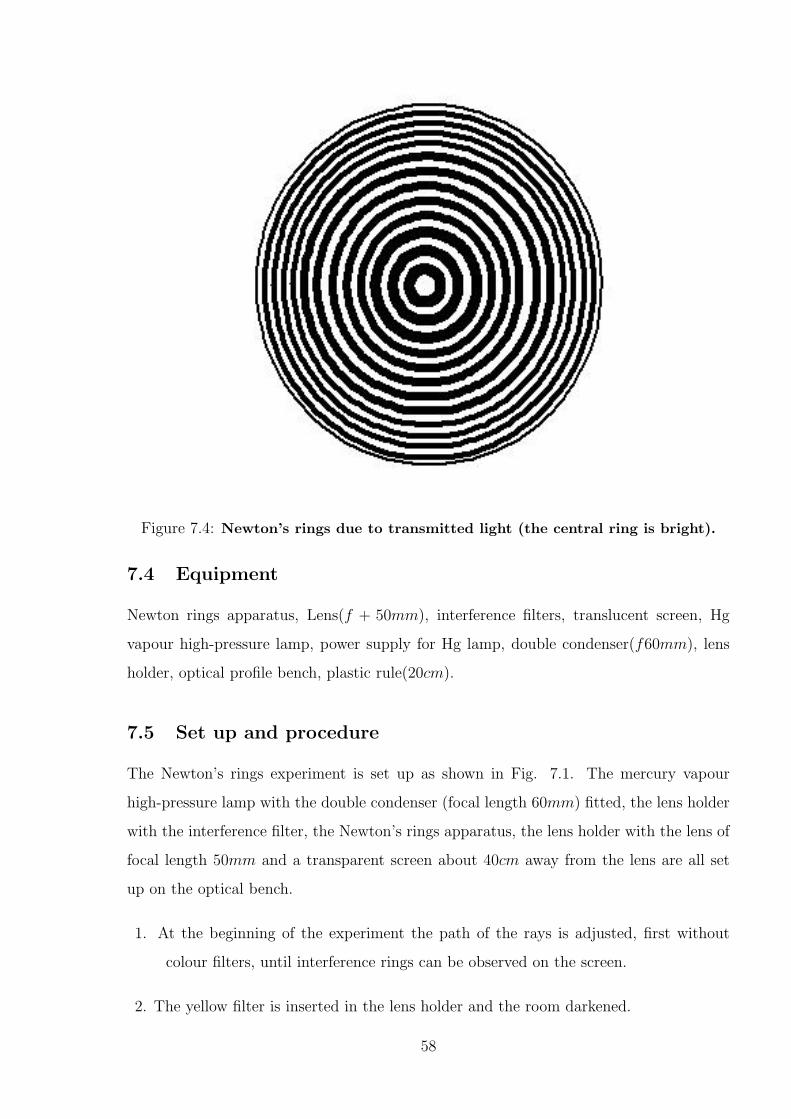
Figure 7.4: Newton’s rings due to transmitted light (the central ring is bright).
7.4 Equipment
Newton rings apparatus, Lens(f + 50mm), interference filters, translucent screen, Hg
vapour high-pressure lamp, power supply for Hg lamp, double condenser(f60mm), lens
holder, optical profile bench, plastic rule(20cm).
7.5 Set up and procedure
The Newton’s rings experiment is set up as shown in Fig. 7.1. The mercury vapour
high-pressure lamp with the double condenser (focal length 60mm) fitted, the lens holder
with the interference filter, the Newton’s rings apparatus, the lens holder with the lens of
focal length 50mm and a transparent screen about 40cm away from the lens are all set
up on the optical bench.
1. At the beginning of the experiment the path of the rays is adjusted, first without
colour filters, until interference rings can be observed on the screen.
2. The yellow filter is inserted in the lens holder and the room darkened.
58
3. By turning the three adjusting screws on the Newton’s rings apparatus to and fro, the
plano-convex lens is set on the plane-parallel glass plate so that the bright centre
of the interference rings is in the mid-point of the millimeter scale projected on the
screen.
• When making this adjustment, ensure that the lens and the glass plate only
just touch. This is achieved when no more rings emerge from the ring centre
when the adjusting screws are tightened up.
4. Measure the diameters Dn of the bright interference rings at the appropriate ordinals.
5. Record the measurements of Dn and the radii rn(=Dn
2) of the rings in table 7.1.
6. Repeat paragraphs 2, 4 and 5 for the blue colour filter at the appropriate ordinals.
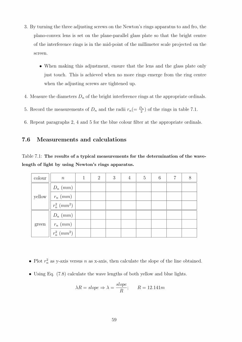
7.6 Measurements and calculations
Table 7.1: The results of a typical measurements for the determination of the wave-
length of light by using Newton’s rings apparatus.
colour
yellow
green
n 1 2 3 4 5 6 7 8
Dn (mm)
rn (mm)
r2n (mm2)
Dn (mm)
rn (mm)
r2n (mm2)
• Plot r2n as y-axis versus n as x-axis, then calculate the slope of the line obtained.
• Using Eq. (7.8) calculate the wave lengths of both yellow and blue lights.
λR = slope⇒ λ =slope
R; R = 12.141m
59
8 Specific charge of the electron - e/me
8.1 Objective
Determination of the specific charge of the electron (e/me) from the path of an electron
beam in crossed electric and magnetic fields of variable strength.
8.2 Principle and Task
Electrons are accelerated in an electric field and enter a magnetic field at right angles
to the direction of motion. The specific charge of the electron is determined from the
accelerating voltage, the magnetic field strength and the radius of the electron orbit.
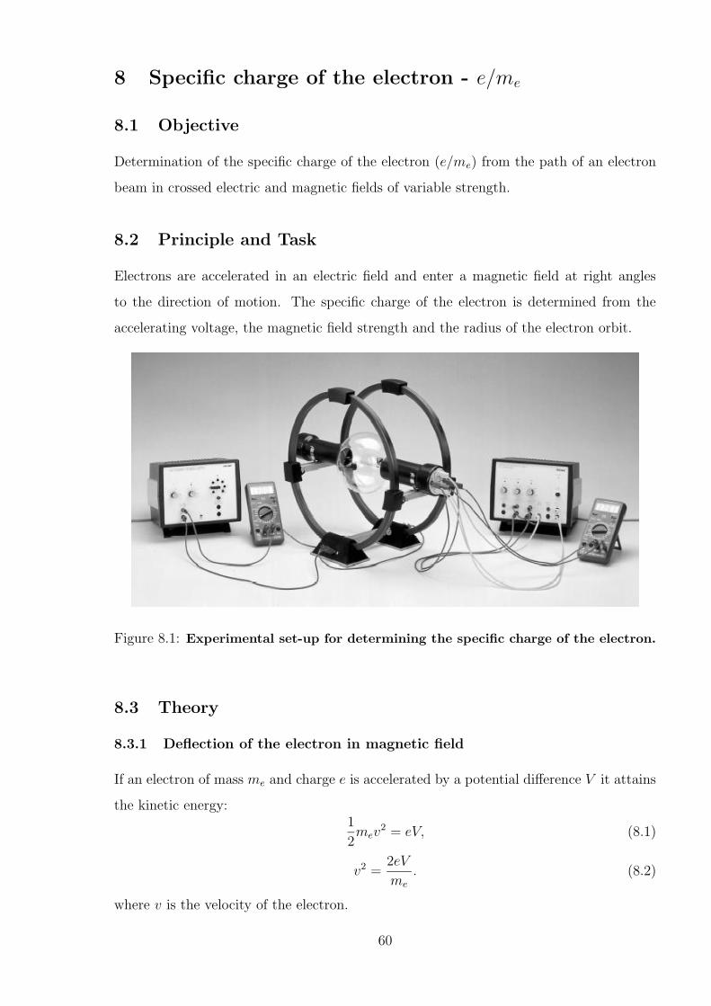
Figure 8.1: Experimental set-up for determining the specific charge of the electron.
8.3 Theory
8.3.1 Deflection of the electron in magnetic field
If an electron of mass me and charge e is accelerated by a potential difference V it attains
the kinetic energy:1
2mev
2 = eV, (8.1)
v2 =2eV
me
. (8.2)
where v is the velocity of the electron.
60
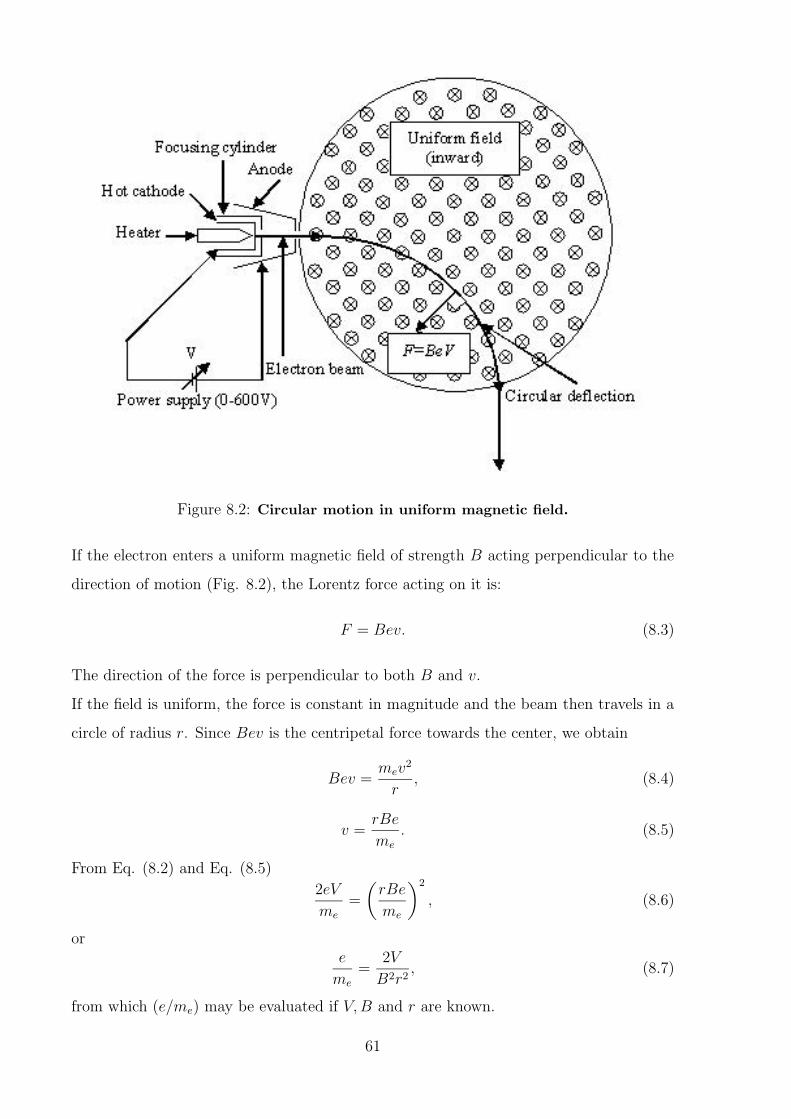
Figure 8.2: Circular motion in uniform magnetic field.
If the electron enters a uniform magnetic field of strength B acting perpendicular to the
direction of motion (Fig. 8.2), the Lorentz force acting on it is:
F = Bev. (8.3)
The direction of the force is perpendicular to both B and v.
If the field is uniform, the force is constant in magnitude and the beam then travels in a
circle of radius r. Since Bev is the centripetal force towards the center, we obtain
Bev =mev
2
r, (8.4)
v =rBe
me
. (8.5)
From Eq. (8.2) and Eq. (8.5)
2eV
me
=
(
rBe
me
)2
, (8.6)
ore
me
=2V
B2r2, (8.7)
from which (e/me) may be evaluated if V,B and r are known.
61
8.3.2 Magnetic field on the axis of a circular coil
To calculate the magnetic field B along the axis of a circular coil, the Biot-Savart law is
used.
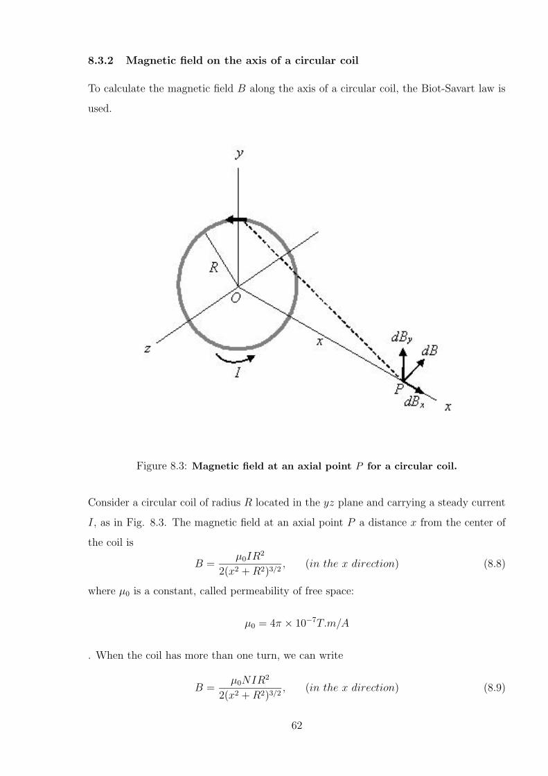
Figure 8.3: Magnetic field at an axial point P for a circular coil.
Consider a circular coil of radius R located in the yz plane and carrying a steady current
I, as in Fig. 8.3. The magnetic field at an axial point P a distance x from the center of
the coil is
B =µ0IR
2
2(x2 +R2)3/2, (in the x direction) (8.8)
where µ0 is a constant, called permeability of free space:
µ0 = 4π × 10−7T.m/A
. When the coil has more than one turn, we can write
B =µ0NIR2
2(x2 +R2)3/2, (in the x direction) (8.9)
62
8.3.3 Helmholtz coils
The field along the axis of a single coil varies with the distance x from the coil. In order
to obtain a uniform field, Helmholtz used two coaxial parallel coils of equal radii(each of
radius R). In this case, when the same current flows round each coil in the same direction,
the resultant field B is uniform for some distance on either side of the point on their axis
midway between the coils. This may be seen roughly by adding the fields due to each coil
alone. Helmholtz coils were used in Thomson’s determination of e/m.
The magnitude of the resultant field B at the mid point can be found from our previous
formula for a coil of N turns(Eq. (8.9)). We now have x = R/2). Thus, for the two coils,
B = 2µ0NIR2
2(R2/4 +R2)3/2=
(
4
5
)3/2µ0NI
R. (8.10)
8.4 Equipment
Narrow beam tube, pair of Helmholtz coils, Power supply(0 − 600V dc), Power sup-
ply(universal), two digital multimeters, Connecting cords.
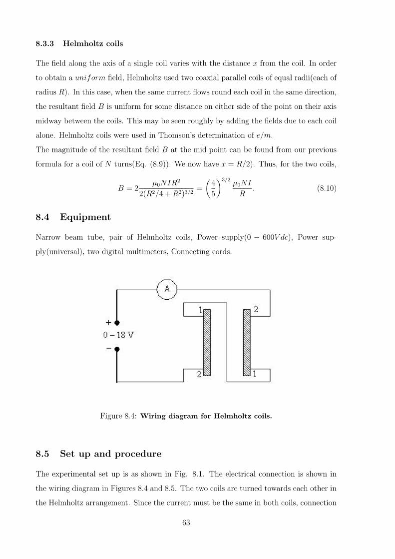
Figure 8.4: Wiring diagram for Helmholtz coils.
8.5 Set up and procedure
The experimental set up is as shown in Fig. 8.1. The electrical connection is shown in
the wiring diagram in Figures 8.4 and 8.5. The two coils are turned towards each other in
the Helmholtz arrangement. Since the current must be the same in both coils, connection
63
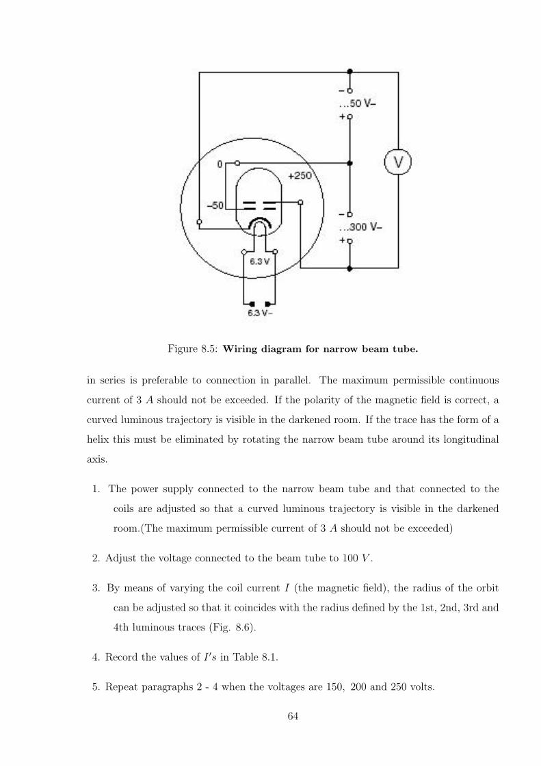
Figure 8.5: Wiring diagram for narrow beam tube.
in series is preferable to connection in parallel. The maximum permissible continuous
current of 3 A should not be exceeded. If the polarity of the magnetic field is correct, a
curved luminous trajectory is visible in the darkened room. If the trace has the form of a
helix this must be eliminated by rotating the narrow beam tube around its longitudinal
axis.
1. The power supply connected to the narrow beam tube and that connected to the
coils are adjusted so that a curved luminous trajectory is visible in the darkened
room.(The maximum permissible current of 3 A should not be exceeded)
2. Adjust the voltage connected to the beam tube to 100 V .
3. By means of varying the coil current I (the magnetic field), the radius of the orbit
can be adjusted so that it coincides with the radius defined by the 1st, 2nd, 3rd and
4th luminous traces (Fig. 8.6).
4. Record the values of I ′s in Table 8.1.
5. Repeat paragraphs 2 - 4 when the voltages are 150, 200 and 250 volts.
64
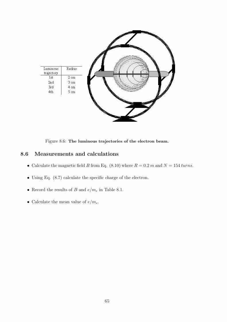
Figure 8.6: The luminous trajectories of the electron beam.
8.6 Measurements and calculations
• Calculate the magnetic fieldB from Eq. (8.10) where R = 0.2m andN = 154 turns.
• Using Eq. (8.7) calculate the specific charge of the electron.
• Record the results of B and e/me in Table 8.1.
• Calculate the mean value of e/me.
65
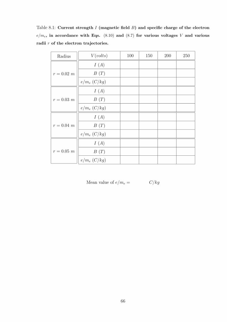
Table 8.1: Current strength I (magnetic field B) and specific charge of the electron
e/me, in accordance with Eqs. (8.10) and (8.7) for various voltages V and various
radii r of the electron trajectories.
Radius
r = 0.02 m
r = 0.03 m
r = 0.04 m
r = 0.05 m
V (volts) 100 150 200 250
I (A)
B (T )
e/me (C/kg)
I (A)
B (T )
e/me (C/kg)
I (A)
B (T )
e/me (C/kg)
I (A)
B (T )
e/me (C/kg)
Mean value of e/me = C/kg
66
9 Diffraction grating
9.1 Objective
1.To determine the wavelengths of the mercury spectral lines using plane transmission
grating.
9.2 Principle and Task
The wave lengths of the spectral lines of a mercury vapour lamp is determined with a
grating spectroscope.
9.3 Theory
Analytical treatment of interference of light due to double slit shows that the intensity at
a point on the screen is given by
I = 4a2 cos2δ
2, (9.1)
where a is the amplitude of the interfered waves and δ is the phase difference.
• When the phase difference δ = n(2π), or the path difference Γ = nλ, where n =
0, 1, 2, 3 · · · , then
I = 4a2. (9.2)
Thus, intensity is maximum when the path difference is a whole number multiple
of wave length.
• When the phase difference δ = (2n + 1)π, or the path difference Γ = (2n + 1) λ2,
where n = 0, 1, 2, 3 · · · , then
I = 0. (9.3)
Thus, intensity is minimum when the path difference is a whole number multiple of
wave length.
9.4 Fraunhofer diffraction at double slit
In Fig. 9.1, AB and CD are two rectangular slit parallel to one another and perpendicular
to the plane of the paper. the width of each slit is a and the width of the opaque portion is
67
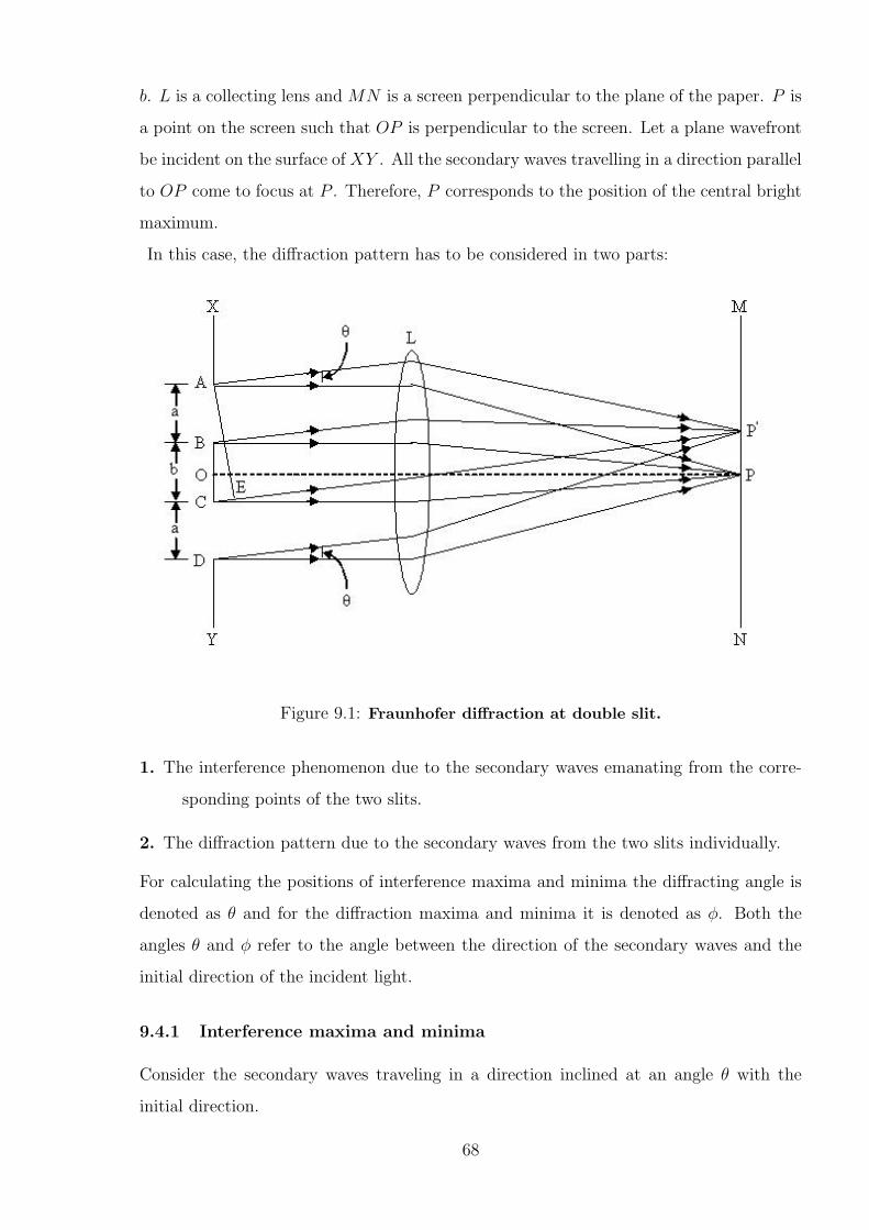
b. L is a collecting lens and MN is a screen perpendicular to the plane of the paper. P is
a point on the screen such that OP is perpendicular to the screen. Let a plane wavefront
be incident on the surface of XY . All the secondary waves travelling in a direction parallel
to OP come to focus at P . Therefore, P corresponds to the position of the central bright
maximum.
In this case, the diffraction pattern has to be considered in two parts:
Figure 9.1: Fraunhofer diffraction at double slit.
1. The interference phenomenon due to the secondary waves emanating from the corre-
sponding points of the two slits.
2. The diffraction pattern due to the secondary waves from the two slits individually.
For calculating the positions of interference maxima and minima the diffracting angle is
denoted as θ and for the diffraction maxima and minima it is denoted as φ. Both the
angles θ and φ refer to the angle between the direction of the secondary waves and the
initial direction of the incident light.
9.4.1 Interference maxima and minima
Consider the secondary waves traveling in a direction inclined at an angle θ with the
initial direction.
68
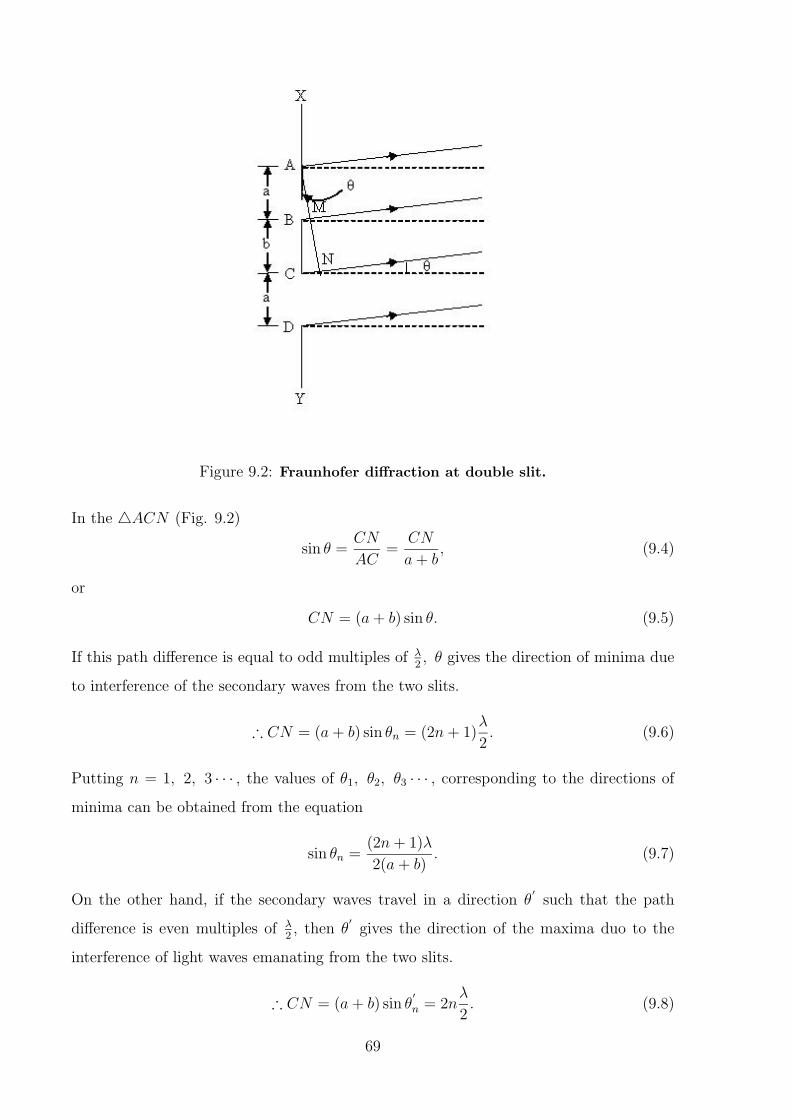
Figure 9.2: Fraunhofer diffraction at double slit.
In the 4ACN (Fig. 9.2)
sin θ =CN
AC=
CN
a+ b, (9.4)
or
CN = (a+ b) sin θ. (9.5)
If this path difference is equal to odd multiples of λ2, θ gives the direction of minima due
to interference of the secondary waves from the two slits.
∴ CN = (a+ b) sin θn = (2n+ 1)λ
2. (9.6)
Putting n = 1, 2, 3 · · · , the values of θ1, θ2, θ3 · · · , corresponding to the directions of
minima can be obtained from the equation
sin θn =(2n+ 1)λ
2(a+ b). (9.7)
On the other hand, if the secondary waves travel in a direction θ′
such that the path
difference is even multiples of λ2, then θ
′
gives the direction of the maxima duo to the
interference of light waves emanating from the two slits.
∴ CN = (a+ b) sin θ′
n = 2nλ
2. (9.8)
69
or
sin θ′
n =nλ
a+ b. (9.9)
Putting n = 1, 2, 3 · · · , the values of θ1, θ2, θ3 · · · , corresponding to the directions of
maxima can be obtained.
From Eq. (9.7)
sin θ1 =3λ
2(a+ b)(9.10)
and
sin θ2 =5λ
2(a+ b), (9.11)
∴ sin θ2 − sin θ1 =λ
a+ b. (9.12)
Thus the angular separation between any two consecutive minima (or maxima) is equal to
λa+b
. The angular separation is inversely proportional to d (= a+ b), the distance between
the two slits.
9.4.2 Diffraction maxima and minima
Consider the secondary waves traveling in a direction inclined at an angle φ with the
initial direction of the initial lights.
If the path BM is equal to λ the wave length of light used, then φ will give the direction
of the diffraction minimum (Fig. 9.2). That is, the path difference between the secondary
waves emanating from the extremities of a slit (i.e., points A and B) is equal to λ.
Considering the wavefront on AB to be made up of two halves, the path difference between
the corresponding points of the upper and lower half is equal to λ2. The effect at P
′
due
to the wavefront incident on AB is zero. Similarly for the same direction of the secondary
waves, the effect at P′
due to the wavefront incident on the slit CD is also zero. In
general,
a sinφn = nλ. (9.13)
Putting n = 1, 2, 3 · · · , the values of φ1, φ2, φ3 · · · , corresponding to the directions of
diffraction minima can be obtained.
9.4.3 Plane transmission diffraction grating
A diffraction grating is an extremely useful device and in one of its form it consists of a
very large number of narrow slits side by side. The slits are separated by opaque spaces.
70
The distance between two slits (a+ b or d) is known as the grating element and it is equal
to the reciprocal of the number of lines per centimeter (N):
d =1
N. (9.14)
When a wavefront is incident on a grating surface, light is transmitted through the slits
and obstructed by the opaque portions. Such a grating is called a transmission grating.
The secondary waves from the positions of the slits interfere with one another, similar to
the interference of waves in Young’s experiment.
9.4.4 Determination of the wave length of a spectral line using plane trans-
mission grating
In the laboratory, the grating spectrum of a given source of light is obtained by using a
spectrometer. Initially all the adjustments of the spectrometer are made and it is adjusted
for parallel rays.
If the source of light emits radiations of different wavelengths, then the beam gets dis-
persed by the grating and in each order a spectrum of the constituent wavelength is
observed. To find the wavelength of any spectral line, the diffracting angles are noted in
the first and the second orders and using the equation
d sin θn = nλ, (9.15)
the wavelength of the spectral line can be calculated.
9.5 Equipment
Spectrometer, lamp holder, spectral lamp Hg, power supply for spectral lamps, diffraction
grating.
9.6 Set up and procedure
The experiment is set up as shown in Fig. 9.3. The spectrometer and the grating should
be adjusted in accordance with the procedure (steps 1-3).
1. Illuminate the slit of the collimator by the mercury light.
71
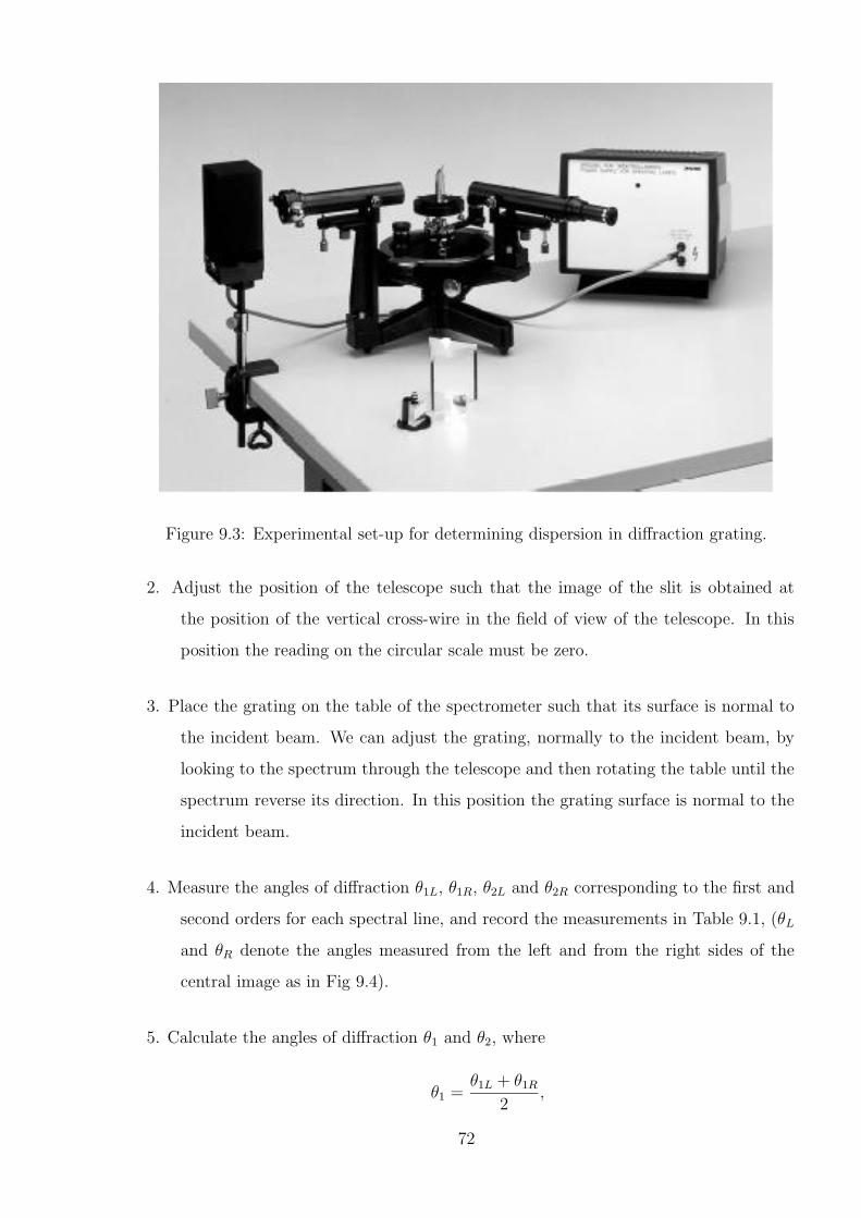
Figure 9.3: Experimental set-up for determining dispersion in diffraction grating.
2. Adjust the position of the telescope such that the image of the slit is obtained at
the position of the vertical cross-wire in the field of view of the telescope. In this
position the reading on the circular scale must be zero.
3. Place the grating on the table of the spectrometer such that its surface is normal to
the incident beam. We can adjust the grating, normally to the incident beam, by
looking to the spectrum through the telescope and then rotating the table until the
spectrum reverse its direction. In this position the grating surface is normal to the
incident beam.
4. Measure the angles of diffraction θ1L, θ1R, θ2L and θ2R corresponding to the first and
second orders for each spectral line, and record the measurements in Table 9.1, (θL
and θR denote the angles measured from the left and from the right sides of the
central image as in Fig 9.4).
5. Calculate the angles of diffraction θ1 and θ2, where
θ1 =θ1L + θ1R
2,
72
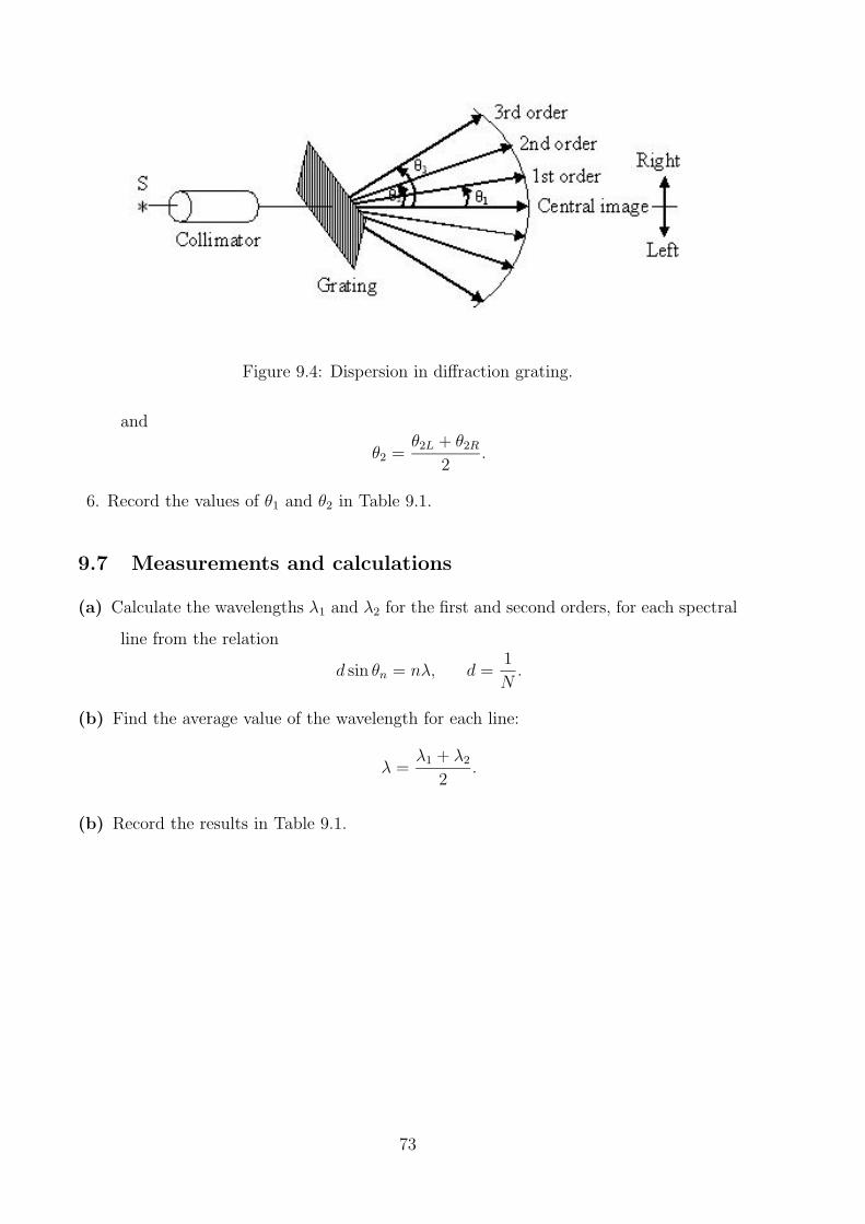
Figure 9.4: Dispersion in diffraction grating.
and
θ2 =θ2L + θ2R
2.
6. Record the values of θ1 and θ2 in Table 9.1.
9.7 Measurements and calculations
(a) Calculate the wavelengths λ1 and λ2 for the first and second orders, for each spectral
line from the relation
d sin θn = nλ, d =1
N.
(b) Find the average value of the wavelength for each line:
λ =λ1 + λ2
2.
(b) Record the results in Table 9.1.
73
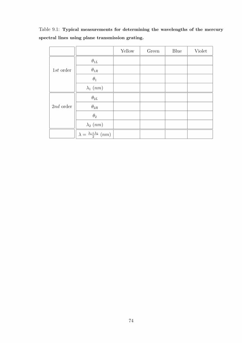
Table 9.1: Typical measurements for determining the wavelengths of the mercury
spectral lines using plane transmission grating.
1st order
2nd order
Yellow Green Blue Violet
θ1L
θ1R
θ1
λ1 (nm)
θ2L
θ2R
θ2
λ2 (nm)
λ = λ1+λ2
2(nm)
74
10 Laws of lenses
10.1 Objective
1. To determine the focal length of an unknown convex lens by measuring the distances
of image and object (using thin lens equation method).
2. To determine the focal length of a convex lens using Bessel’s method.
10.2 Principle and Task
The focal lengths of unknown lenses are determined by measuring the distances of image
and object and by Bessel’s method.
10.3 Theory
The focal length of a lens can be determined by several techniques. Some of these are less
difficult to use than others and some are more accurate. The following two subsections
are a brief description of some of the techniques.
10.3.1 Thin Lens Equation
The relationship between the focal length f of a lens, the object distance u and the image
distance v is obtained from geometrical optics. Three particular rays, the focal ray, the
parallel ray and the central ray, are used to construct the image (Fig. 10.1). From the
laws of similar triangles,I
O=
v
u(10.1)
andO
I=
f
v − f(10.2)
where I is the image size and O is the object size. From Eq. (10.3.1) and Eq. (10.3.2),
we can writeu
v=
f
v − f⇒ uv − uf = vf ⇒ uv = (u+ v)f, (10.3)
from which we obtain the lens formula
1
f=
1
u+
1
v, (10.4)
75
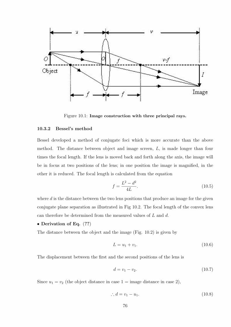
Figure 10.1: Image construction with three principal rays.
10.3.2 Bessel’s method
Bessel developed a method of conjugate foci which is more accurate than the above
method. The distance between object and image screen, L, is made longer than four
times the focal length. If the lens is moved back and forth along the axis, the image will
be in focus at two positions of the lens; in one position the image is magnified, in the
other it is reduced. The focal length is calculated from the equation
f =L2 − d2
4L. (10.5)
where d is the distance between the two lens positions that produce an image for the given
conjugate plane separation as illustrated in Fig 10.2. The focal length of the convex lens
can therefore be determined from the measured values of L and d.
• Derivation of Eq. (??)
The distance between the object and the image (Fig. 10.2) is given by
L = u1 + v1. (10.6)
The displacement between the first and the second positions of the lens is
d = v1 − v2. (10.7)
Since u1 = v2 (the object distance in case 1 = image distance in case 2),
∴ d = v1 − u1. (10.8)
76
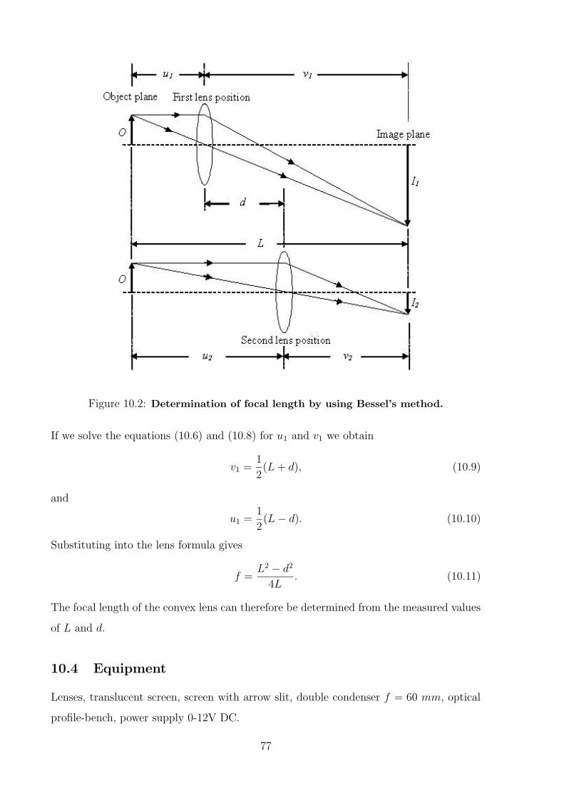
Figure 10.2: Determination of focal length by using Bessel’s method.
If we solve the equations (10.6) and (10.8) for u1 and v1 we obtain
v1 =1
2(L+ d), (10.9)
and
u1 =1
2(L− d). (10.10)
Substituting into the lens formula gives
f =L2 − d2
4L. (10.11)
The focal length of the convex lens can therefore be determined from the measured values
of L and d.
10.4 Equipment
Lenses, translucent screen, screen with arrow slit, double condenser f = 60 mm, optical
profile-bench, power supply 0-12V DC.
77
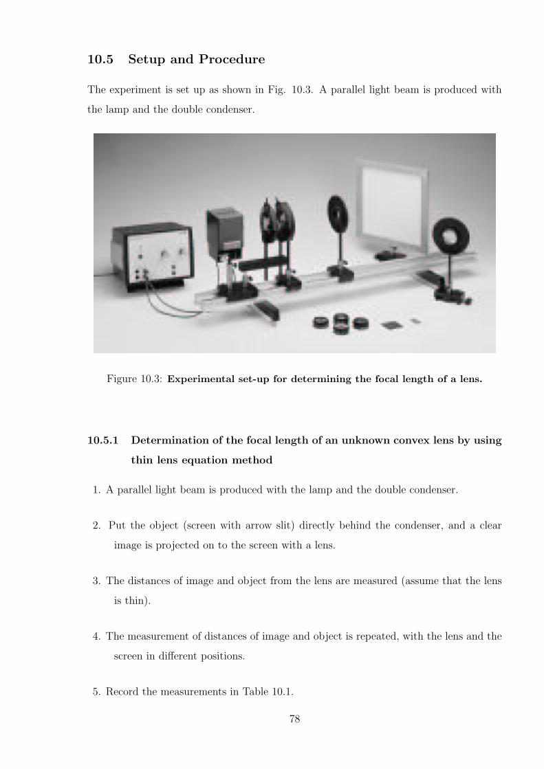
10.5 Setup and Procedure
The experiment is set up as shown in Fig. 10.3. A parallel light beam is produced with
the lamp and the double condenser.
Figure 10.3: Experimental set-up for determining the focal length of a lens.
10.5.1 Determination of the focal length of an unknown convex lens by using
thin lens equation method
1. A parallel light beam is produced with the lamp and the double condenser.
2. Put the object (screen with arrow slit) directly behind the condenser, and a clear
image is projected on to the screen with a lens.
3. The distances of image and object from the lens are measured (assume that the lens
is thin).
4. The measurement of distances of image and object is repeated, with the lens and the
screen in different positions.
5. Record the measurements in Table 10.1.
78
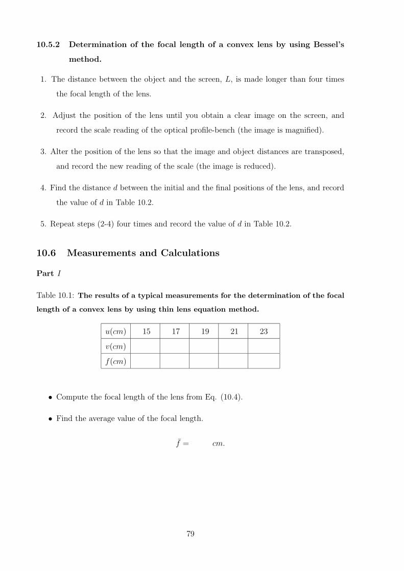
10.5.2 Determination of the focal length of a convex lens by using Bessel’s
method.
1. The distance between the object and the screen, L, is made longer than four times
the focal length of the lens.
2. Adjust the position of the lens until you obtain a clear image on the screen, and
record the scale reading of the optical profile-bench (the image is magnified).
3. Alter the position of the lens so that the image and object distances are transposed,
and record the new reading of the scale (the image is reduced).
4. Find the distance d between the initial and the final positions of the lens, and record
the value of d in Table 10.2.
5. Repeat steps (2-4) four times and record the value of d in Table 10.2.
10.6 Measurements and Calculations
Part I
Table 10.1: The results of a typical measurements for the determination of the focal
length of a convex lens by using thin lens equation method.
u(cm) 15 17 19 21 23
v(cm)
f(cm)
• Compute the focal length of the lens from Eq. (10.4).
• Find the average value of the focal length.
f̄ = cm.
79
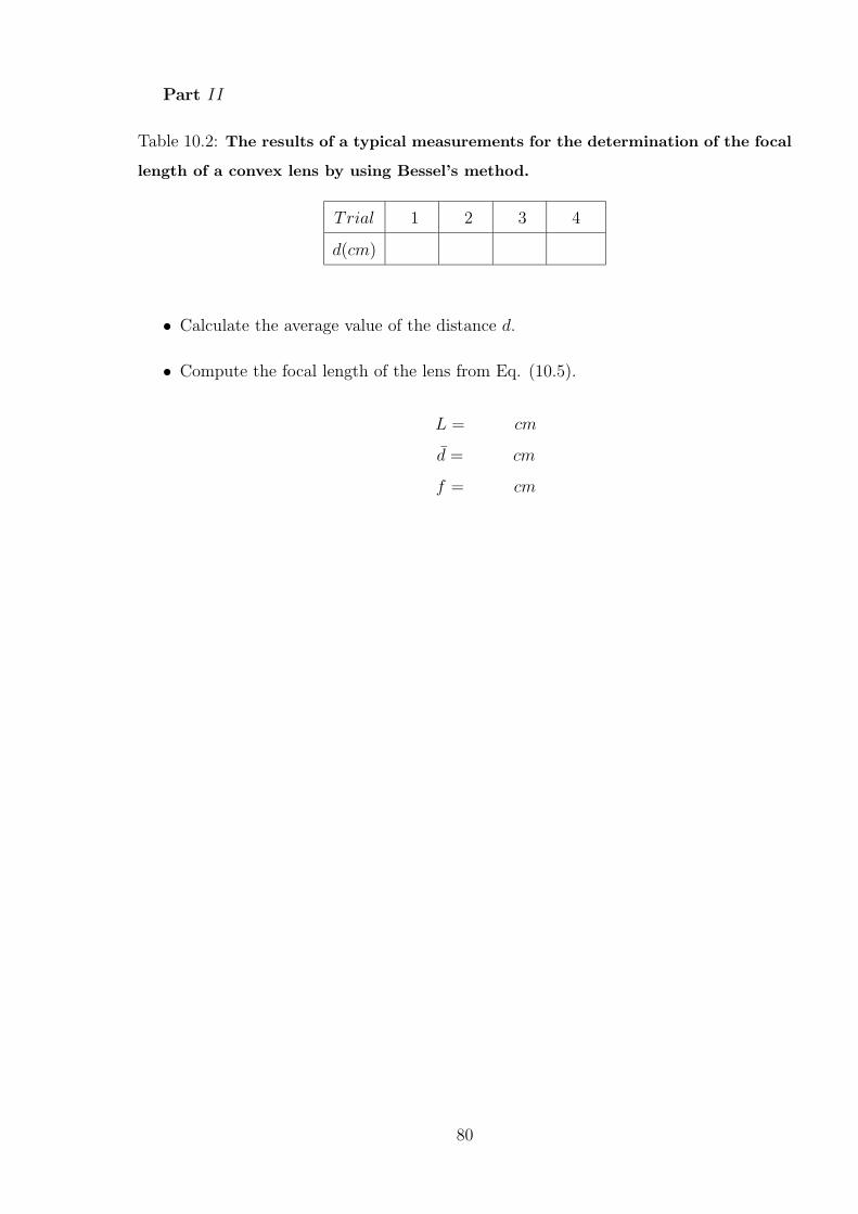
Part II
Table 10.2: The results of a typical measurements for the determination of the focal
length of a convex lens by using Bessel’s method.
Trial 1 2 3 4
d(cm)
• Calculate the average value of the distance d.
• Compute the focal length of the lens from Eq. (10.5).
L = cm
d̄ = cm
f = cm
80
![Lecture 9. Input and output - Functional Programming[FacultyofScience InformationandComputingSciences] 3 Interactiveprograms Intheolddays,allprogramswerebatch programs Introducetheprogramandinput,sitanddrink](https://img.pdfslide.us/doc/110x75/60b7eb97c7c5cb6b1819f445/lecture-9-input-and-output-functional-facultyofscience-informationandcomputingsciences.jpg)


![Lecture 13. More monads and applicatives - Functional ...[FacultyofScience InformationandComputingSciences] 25 Anotheruseforstate:counters Givenabinarytree,returnanewonelabelledwithnumbers](https://img.pdfslide.us/doc/110x75/6099c0f1535ef758e36e29aa/lecture-13-more-monads-and-applicatives-functional-facultyofscience-informationandcomputingsciences.jpg)