Embed Size (px)
Citation preview

Laboratory Testing for Adfreeze Bond of Sand on Model
Steel Piles
Joey Villeneuve, B. Sc.A.
Thesis submitted in partial fulfillment of the requirements for the
Master of Applied Science degree in Civil Engineering
Under the supervision of
Dr. Julio Angel Infante Sedano, P. Eng
Department of Civil Engineering
University of Ottawa
Ottawa, Ontario
© Joey Villeneuve, Ottawa, Canada, 2018

ii | P a g e
Abstract
Abstract
This study explored the available adfreeze data published in literature and the techniques used to
obtain it. Two methods were selected and modified to complete series of adfreeze bond test. A
model pile pull-out method consisting of pulling a pile out a large specimen of soil was the first
method used. The second method was modified from an interface shearing apparatus developed
by Dr. Fakharian and Dr. Evgin at the University of Ottawa in 1996 and allowed preparing,
freezing and testing the specimen in place.
The material and soil tested for this study were provided by EXP Services Inc. The model pile, a
galvanized HSS 114.3 x 8.6 section, is commonly used to install solar panels. Soil was taken
from a future solar farm site in proximity to Cornwall, Ontario.
The study had for objective to develop a low cost adfreeze laboratory testing method.
Limitations of the technics and apparatus used were observed. While the results of a model pile
pull-out test compared to previous data publish by Parameswaran (1978), the interface shear
series of test presented more limitations. The interface shearing method has been previously
study by Ladanyi and Thériault (1990).
Issues with the interface shear method due to the water content of the soil as well as the range of
normal stress applied to the specimen both during testing and freezing. The data obtained was
inconclusive and the method will be studied in future research program.
This studied approach the adfreeze testing with new improvement. The main contribution of this
study is the data obtained by measuring and observing adfreeze of ice poor sand with varying
water content. The measurements allowed to study the effect that increasing water content has on
the interface bond strength.
The modifications made to interface shear apparatus are also major new contribution provided by
this research. The apparatus was converted in a small freezer chamber using insulation panel and
vortex tubes. Which was used to freeze the specimen in the testing chamber and testing adfreeze
in place without handling the shear box arrangement.
iii | P a g e
Acknowledgements
Acknowledgements
The author would like to express his most sincere appreciation to his research supervisor, Dr.
Julio Angel Infante Sedano, for his great support, knowledge, help and guidance throughout the
preparation, design, setup and test series. Dr. Infante Sedano was an invaluable member of the
group that help put this research together.
The author also wishes to thank Dr. Sai Vanapalli, Dr. Mamadou Fall and Dr. Mohammad
Rayhani for serving as members of the examination committee.
The author would also like to thank his laboratory assistant Mathieu Villeneuve, Camille
Montour and Frederik Hupe for their long hours spent in the laboratories and the help they
brought in the preparation of the specimen.
Thank you to the staff of the department of Civil Engineering of the University of Ottawa for
their help and particularly to Mr. Jean Claude Celestin and Mr. Muslim Majeed for their
exception technical knowledge and support.
Nothing would have been possible without the financial support of the University of Ottawa and
EXP Services Inc. with Mr. Mansour Navidpour who provided the material.
Thank you to all.

iv | P a g e
Table of Content
Table of Content
Abstract ........................................................................................................................................... ii
Acknowledgements ........................................................................................................................ iii
Table of Content ............................................................................................................................ iv
Table of Figures ........................................................................................................................... vii
Table of Tables ............................................................................................................................... x
Chapter 1. INTRODUCTION .................................................................................................... 1
1.1. Problem Statement ____________________________________________________ 2
1.2. Objectives ___________________________________________________________ 3
1.3. Scope of Research _____________________________________________________ 4
1.4. Outline of Thesis ______________________________________________________ 4
Chapter 2. Literature Review ..................................................................................................... 6
2.1. Frozen ground _______________________________________________________ 6
2.2. Soil Temperature Observation __________________________________________ 8
2.3. Frozen Ground Sampling _____________________________________________ 10
2.4. Freezing process _____________________________________________________ 11
2.5. Effect of pore water pressure __________________________________________ 14
2.6. Rheology of soil and ice mixture ________________________________________ 17
2.7. Frost Heaving _______________________________________________________ 21
2.8. Adfreeze____________________________________________________________ 23
2.9. Ground freezing applications __________________________________________ 25
2.10. Adfreeze testing by push through _______________________________________ 28
2.11. Adfreeze testing by interface shearing ___________________________________ 30
2.12. Adfreeze relation to shear strength _____________________________________ 33
2.13. Conclusion and direction ______________________________________________ 34
Chapter 3. Model pile pull-out test .......................................................................................... 36
3.1. Introduction ________________________________________________________ 36
3.2. Pull-out apparatus ___________________________________________________ 36
v | P a g e
Table of Content
3.3. Tested soil properties _________________________________________________ 39
3.4. Sample preparation __________________________________________________ 41
3.5. Test Settings ________________________________________________________ 43
3.6. Test results _________________________________________________________ 44
3.7. Observations ________________________________________________________ 48 3.7.1. Fragile bond ....................................................................................................................................... 48 3.7.2. Effective bond depth ......................................................................................................................... 49
Chapter 4. Soil Interface Testing ............................................................................................. 50
4.1. Introduction ________________________________________________________ 50
4.2. Soil-Interface apparatus ______________________________________________ 50
4.3. Freezing equipment __________________________________________________ 53 4.3.1. Refrigeration panels .......................................................................................................................... 53 4.3.2. Vortex tubes ...................................................................................................................................... 54
4.4. Test surface _________________________________________________________ 55
4.5. Sample Preparation __________________________________________________ 58
4.6. Test Settings ________________________________________________________ 60
4.7. Test results _________________________________________________________ 61
4.8. Observations ________________________________________________________ 64 4.8.1. Reproducibility .................................................................................................................................. 64 4.8.2. Moisture seepage and sample consolidation ...................................................................................... 65 4.8.3. Boundary effect ................................................................................................................................. 65 4.8.4. Apparatus limitations ........................................................................................................................ 66
Chapter 5. Testing method discussion ..................................................................................... 68
5.1. Pull out test discussion ________________________________________________ 68 5.1.1. Field representation ........................................................................................................................... 68 5.1.2. Test versatility ................................................................................................................................... 69 5.1.3. Test results ......................................................................................................................................... 70 5.1.4. Testing equipment ............................................................................................................................. 70
5.2. Soil Interface testing discussion ________________________________________ 70 5.2.1. Field representation ........................................................................................................................... 71 5.2.2. Test versatility ................................................................................................................................... 71 5.2.3. Test results ......................................................................................................................................... 72 5.2.4. Testing equipment ............................................................................................................................. 72
6.3 Data discussion ______________________________________________________ 72
Chapter 6. Conclusion .............................................................................................................. 75
7.1 Suggestion for further studies ____________________________________________ 76
References .................................................................................................................................... 77
Appendix A. Pull out test results ............................................................................................. 82

vi | P a g e
Appendix B. Interface test results ........................................................................................... 97
Appendix C. Pull out Setup Drawings .................................................................................. 118

vii | P a g e
Table of Figures
Table of Figures
Figure 1: Distribution of frozen ground in the Northern Hemisphere (from Zhang et al., 2003) _________________ 7
Figure 2: Typical permafrost ground temperature (from Andersland, 2004) ________________________________ 8
Figure 3: Frost tube for measurement of rate and depth of thaw or seasonal frost penetration (Ladanyi and Johnston,
1978) _______________________________________________________________________________________ 9
Figure 4: Removing a sample from a core barrel (SnowNet, 2009) ______________________________________ 11
Figure 5: Soil freezing characteristic curve of sandy loam (from Stähli, 2005) _____________________________ 12
Figure 6: Similarity of the SWC and SFC for a laboratory tested silty loam (from Stähli, 2005) _______________ 14
Figure 7: Water phase diagram (by: Christopher Auyeung) ____________________________________________ 15
Figure 8: Failure mechanism map of unconfined compressive strength of frozen Ottawa sand at -7ºC and a constant
strain rate of 4.4 x 10⁻⁴ s-1 (From Andersland, 2004) _________________________________________________ 17
Figure 9: Relationship between uniaxial compressive strength of frozen sand with temperature at different water
content. (Ladanyi, 2003) _______________________________________________________________________ 19
Figure 10: Stress-strain behavior of ice under different strain rate A) ductile behavior with strain hardening, B)
dilatant behavior with strain softening, C) brittle behavior with failure after yield point, D) brittle failure (Arenson et
al., 2007) ___________________________________________________________________________________ 20
Figure 11: Stress response of frozen ground as a function of strain rate and volumetric ice content (Arenson et al.,
2007) ______________________________________________________________________________________ 20
Figure 12: Ice formation in soils: (a) closed system (b) open system (c) drainage layer (from Andersland, 2004) __ 22
Figure 13: Pile foundations bearing capacity schematic in permafrost (from Parameswaran, 1978) _____________ 24
Figure 14: Adfreeze load-displacement curves for piles in frozen sand: (A) untreated B.C. fir, (B) painted steel and
(C) concrete (from Parameswaran,1978) __________________________________________________________ 25
Figure 15: Ground freezing tube (freeze pile) (Andersland, 2004) ______________________________________ 26
Figure 16: Ground freezing tubes used to excavate (a) tunnel (Frank Coluccio Construction, 1996) and (b) shaft
(BDF, 2009) ________________________________________________________________________________ 27
Figure 17: Duct-Ventilated fill foundation (ZHDC,2011) _____________________________________________ 28
Figure 18: Schematic diagram of push through testing apparatus (Parameswaran, 1978) _____________________ 29
Figure 19: Adfreeze bond of frozen sand against steel express in function of shear strength of the frozen sand (T=-2
°C) (Ladanyi & Thériault, 1990) ________________________________________________________________ 32

viii | P a g e
Table of Figures
Figure 20: Longitudinal cross-section of the double shear apparatus: 1. Vertical load application; 2. Loading platen;
3. Porous stone; 4. Cylindrical bearings; 5. Antifreeze out; 6. Horizontal load application; 7. Thermistor; 8. Ball
bearing; 9. Upper shear ring; 10. Central shear ring; 11. Antifreeze in; 12. Lower shear ring (from Ladanyi and
Thériault,1990) ______________________________________________________________________________ 33
Figure 21: Galdabini Sun 60 set up with frozen soil test box ___________________________________________ 37
Figure 22: Linear potentiometer schematic (http://www.instrumentationtoday.com) ________________________ 38
Figure 23: Pile pull arm attachment set up full view (left), cut view (right) _______________________________ 38
Figure 24: Cornwall sand Grain size distribution ____________________________________________________ 40
Figure 25: Proctor and static compaction curve _____________________________________________________ 41
Figure 26: Waterproof DS18B20 Digital temperature sensor (Adafruit) __________________________________ 42
Figure 27: Attachment and LPT set up to the model pile ______________________________________________ 43
Figure 28: Typical force-displacement curve results _________________________________________________ 44
Figure 29: Proctor vs tested dry densities __________________________________________________________ 46
Figure 30: Adfreeze Strength in Function of Moisture Content _________________________________________ 46
Figure 31: Adfreeze strength in function of density __________________________________________________ 47
Figure 32: Adfreeze strength in function of embedded depth___________________________________________ 48
Figure 33: Soil interface separation at the surface of the sample ________________________________________ 49
Figure 34: Schematic of Fakharian's 3D interface apparatus (C3DI) (from Fakarian & Evgin, 1996)____________ 51
Figure 35: Foam insulation panel covering the testing chamber of the C3DI ______________________________ 52
Figure 36: Interface testing table inside the insulated chamber _________________________________________ 53
Figure 37: Colling equipment: Igloo Iceless Thermoelectric Cooler (left) (Terapeak.com), Exair vortex tube (rigth)
(exair.com) _________________________________________________________________________________ 54
Figure 38: Vortex tube output (modified from Streamtek.com) _________________________________________ 55
Figure 39: Hommel tester T500 Roughness meter (http://granat-e.ru/t500) ________________________________ 56
Figure 40: Roughness profile with average roughness (Hommel) _______________________________________ 56
Figure 41: Roughness profile with maximum roughness (Hommel) _____________________________________ 57
Figure 42: Roughness profile with average peak roughness (Hommel) ___________________________________ 57
Figure 43: Shear box with Teflon layer (left); Sample being compacted in load frame with proving ring(centre);
Sample after compaction (right) _________________________________________________________________ 59

ix | P a g e
Table of Figures
Figure 44: Interface testing relationship between moisture content and adfreeze stress in function of normal stress 63
Figure 45: Interface testing relationship between normal stress and adfreeze stress in function of sample moisture
content ____________________________________________________________________________________ 64
Figure 46: Sample deformation due to border effect _________________________________________________ 66
Figure 47: Field pull test set up (left) lab pull out test (right) ___________________________________________ 69
Table of Figures

x | P a g e
Table of Tables
Table of Tables
Table 1: Values for peak adfreeze strength for various pile type under constant shear rate (Parameswaran, 1978) _ 30
Table 2: Shear to adfreeze bond coefficient presented by Weaver and Morgenstern (1981) ___________________ 34
Table 3: Soil grading coefficients ________________________________________________________________ 40
Table 4: Pull-out test summary __________________________________________________________________ 45
Table 5: Roughness measurement of tested pile and various galvanized steel plates and sheeting ______________ 58
Table 6: Interface shear test results_______________________________________________________________ 62
Table 7: Preliminary interface test series results ____________________________________________________ 63
Table of Tables

1 | P a g e
INTRODUCTION
Chapter 1. INTRODUCTION
Given that the greater part of Canada’s territory is situated north of the 49th parallel, it
experiences some of the hardest winters in the world. The frost seasons are therefore very long
and even continuous in some part of the country. Because of this, the formation of frozen soil is
then unavoidable. In the northernmost latitudes, part of the frozen soil remains frozen year-round
leading to the formation of permafrost. Since 50% of the country is covered by some type of
Permafrost (Harris S.A, 2015), studies of frozen soils are therefore relevant to the Canadian
reality.
Permafrost is a soil condition for which, by definition, the soil needs to remain permanently
frozen for at least 2 consecutive freezing seasons (or 2 years). This type of soil condition can be
found north of the 50th parallel or in high mountain ranges. On the other hand, the frost front can
be observed at latitudes as low as the 40th parallel in North America and down to the 30th
parallel in Asia (Phukan, 1978). The seasonal ground freezing limit is defined by engineers by a
frost penetration depth of 300mm (Andersland, 2004). Canada, Russia and Greenland have the
biggest permafrost cover of the entire world: 50%, 60%, and 100% of their total area
respectively. In other countries, such as the Scandinavian nations, Western Europe, the United
States and China, engineers have to contend with seasonally frozen ground. The study of frozen
soil needs a different approach than the classical soil mechanics. A fourth solid phase is found in
frozen soil: ice. This fourth phase combined with the three classical phases (solid soil, water and
air) at different ratios will modify the original soil properties.
Frozen ground has a very broad definition. Most simply, it is defined as a soil or a rock at a
temperature below 0°C, independent of the water content (Andersland, 2004). Even if this
definition includes dry soils, frozen soils are generally considered to consist of four phases: soil
grains, ice, unfrozen water and gas. The ice, in any concentration, is an important bonding agent
that fuses the soil or rock particles together similarly to cement in concrete. It increases shear
strength and makes the soil impervious to water seepage.

2 | P a g e
INTRODUCTION
Frozen soil mechanics is a relatively young field of geotechnical engineering. The earliest
research in the domain dates back to the 1960s. Major advances were made during the mid-1970s
and 1980s, when demand for petroleum lead the industry into northern latitudes (Arenson et al.,
2007). These studies brought the first design criteria for foundations, pavements and
investigation methods for frozen soils. However, the late 1980s depression delayed new research
for nearly a decade (1990s). It was not until the mid-2000s that interest for the domain arose
anew.
Frozen soils are still not well understood today. Researchers such as Andersland, Arenson,
Ladanyi and Morgensten have pioneered the domain and explored practical fields and theoretical
aspects of it. It was quickly found that classical soil mechanics was not representative of frozen
soil conditions. The presence of ice as a bonding agent not only influences strength and
permeability, but particle interaction and internal stress distribution.
1.1. Problem Statement
Many types of piles have been used in permafrost. The range of material used includes timber,
steel and concrete (Heydinger, 1987). Steel H-piles, corrugated metal piles and circular HSS
piles are the types most commonly used. Timber piles are usually tapered with the tip downward
to facilitate installation or upwards when greater uplift resistance is needed. (Crory, 1966) Pre-
tensioned precast concrete piles are manufactured to withstand handling and driving stress. Cast
in place concrete piles are not recommended due to the heat emitted during curing. The most
advanced type of piling systems now used includes freeze pile and thermosyphon. Freeze piles
are formed with interior tubing allowing cooling fluid to circulate and evacuate heat from the
ground therefore maintaining it frozen. Thermosyphon piles are sealed with an anti-freeze fluid
which boils at the target ambient temperature. The vapour thus formed transports the excess heat
to the surface where the fluid condenses and flows back in the pile. The heat is then dissipated at
the surface, and the soil surrounding the pile remains frozen.
Canada has a standard for thermosyphon pile design, CAN/CSA-S500-14; Thermosyphon
foundations for buildings in permafrost regions and a standard for permafrost protection
CAN/CSA S501-14; Moderating the Effects of Permafrost Degradation on Existing Building
3 | P a g e
INTRODUCTION
Foundations but no frozen soil foundation design standard exists. The Canadian Foundation
Engineering Manual doesn't cover any design aspect of deep foundations in frozen soil
conditions with the exception of frost heave and frost susceptible soils. It provides a general
value for adfreeze of 65 to 100 kPa for fine grain soils and 150 kPa for saturated frozen gravel.
Experience is the only guideline in frozen ground foundations.
It is well known that pile foundations in frozen soil conditions rely mainly on the adfreeze bond
to carry loads and the end bearing capacity is generally neglected (Ladanyi and Theriault, 1990).
The implication is that in the active zone (the area subjected to freezing and thawing cycles), the
combined effect of the adfreeze bond, and the expanding nature of freezing water can lead to an
upward force acting through the structure's foundation piles. The adfreeze force can be so large
that the entire structure can be lifted without it touching the ground.
A considerable amount of information and observations are available on the adfreeze bond of
specific soils, but little applicable design methods and standard testing methods. Therefore, this
research looked into comparing results of two different testing techniques similar to the ones
found in literature. The testing also observed the effect of the adfreeze bond on ice poor soils,
considering specimens with different water contents before freezing, as well as different net
normal stresses.
1.2. Objectives
The objectives of this study were to;
1) Put in place a pull-out testing procedure, easy to implement in laboratory. Achieving
cheap and easy laboratory testing method to demonstrate the potential of adfreeze testing.
2) Measure and observe adfreeze bond strength. While there is various research presenting
measured adfreeze values, there is still gaps in the data and observation.
3) Use an interface testing apparatus to test adfreeze bond under direct shear. Modified
direct shear box have previously been used to test interface friction.
4) Create an apparatus able to freeze and test specimens in place limiting handling of fragile
samples.

4 | P a g e
INTRODUCTION
5) Test and compare pull-out and direct shear procedures in interface apparatus.
1.3. Scope of Research
The objectives of this research described in the previous section were achieved at the
Geotechnical Laboratory and the Structural Laboratory of the University of Ottawa. Adfreeze
bond was measured and observed by a Universal Testing Machine (UTM) and a Cyclic 3-D
Simple Shear Apparatus for interface testing.
The testing procedures for pull-out testing was developed using easy to procure material such as
off the shelf thermistors, shop fabricated steel elements and a commercial freezer. The
observation and data of this new adfreeze testing method where compared to the data and
observation from literature push-through testing.
The interface test series relied on a freeze/test in place sequence developed specifically for the
current adfreeze testing program. The results and observations of the data were compared to
available literature data obtained using a comparable interface testing method.
The present study covered adfreeze bond testing for a pile shape and material commonly used for
solar panel installation in a soil provided by a consultant studying the feasibility of a solar park
near the municipality of Cornwall, Ontario. The novelty of the testing program relied on the
adfreeze tests that were conducted.
1.4. Outline of Thesis
This thesis is arranged in chapters dividing the different testing method and finale discussion of
the results. “Chapter 2: Literature Review” presents a summary review on previous knowledge of
frozen ground. The key topics of review covered research and testing of adfreeze bond, soil
freezing process and effect of water/ice content.
“Chapter 3: Model pile pull-out test” presents the soil, material and equipment used for a model
pile pull-out testing program. This section presents the detailed procedure for large specimen

5 | P a g e
INTRODUCTION
preparation and freezing as well as the apparatus setting. The results and observations of the test
program as summarized at the end.
“Chapter 4: Soil Interface Testing” presents the material relation used for interface and model
pile testing as well as the equipment used to determine the comparison. The important
modification made to the apparatus to allow freeze/test in place are detailed. The chapter
concludes with the observation and results obtained from the series of tests.
“Chapter 5: Testing method discussion” discusses the observation made during each testing
procedures and the issues encountered. This section presents the feasibility of low cost adfreeze
testing by comparing results with known values and discussion available in literature.
“Chapter 6: Conclusion” presents a summary and conclusion of the research program. Some
recommendations for further research on the subject are also summarized.
Appendices show all the detailed data collected from the testing procedures as well as shop
drawings for the fabricated equipment used during the pull-out tests.
− Appendix A: presents the individual test results of the pull-out test series
− Appendix B: presents the individual test results of the shear interface test series
− Appendix C: presents the set-up and material drawing for the pull-out test series

6 | P a g e
Literature Review
Chapter 2. Literature Review
The studies introduced in Chapter 1 lead to the first design criteria for foundations, pavements
and investigation methods for frozen soils. Due to the late ‘80s depression it was not until the
mid-2000s that new interest for the domain manifested itself.
Adfreeze or pile-soil interface bond is the main contributor to frozen ground bearing capacity. It
is also a component resisting the heave forces in permafrost regions (Parameswaran, 1978).
However, while designing piles and other types of foundations in seasonally frozen ground, the
active layer is mostly ignored. Designers assume no influence from the active layer and simply
design from under the assumed. Some exceptions are found depending on the project
specifications.
2.1. Frozen ground
Frozen ground or frozen soil is defined as:
“Soil or rock with a temperature below 0°C” (Andersland, 2004)
or
“Ground with a mean soil temperature below the freezing point” (Zang et al., 2003)
These definitions encompass all soils and rock with a temperature below the freezing point of
water independently of their water content. Although the definition includes dry soils, frozen
soils are generally considered to be composed of four phases: soil grain, ice, unfrozen water and
gas. The ice, in any concentration, is an important bonding agent that fuses the soil or rock
particles together as cement does for concrete. Thus, it increases shear strength and makes the
soil impervious to water seepage.
The large increase of soil strength is commonly used by construction engineers designing for
frozen soils. Excavations and slopes are more stable, the bearing capacity of foundations is

7 | P a g e
Literature Review
increased, and contaminants are locally constrained by ice. These are some of the advantages of
working with frozen soils. Its major disadvantage, however, is that a frozen soil quickly loses its
improved properties when thawing.
Figure 1: Distribution of frozen ground in the Northern Hemisphere (from Zhang et al.,
2003)
The strongest frozen soil condition is known as permafrost. It is often described as a unique
material. Permafrost is defined as a soil condition where the soil needs to be permanently frozen
for at least 2 consecutive freezing seasons (or 2 years). On the other hand, seasonal ground
freezing limit is defined by engineers by a frost penetration depth of 300 mm (Andersland,
2004).
According to Zhang (2003) permafrost covers 25.6% of the land in the Northern Hemisphere,
which is approximately 24.91 million square kilometers while seasonally frozen ground coverage
is about 50.5%, which represents 48.12 million square kilometers. Another 6.6% (6.27 millions
square kilometer) is defined as “intermittently frozen ground”. Intermittently frozen ground is a
near surface freezing during 1 to 15 days of the year. Figure 1 demonstrates the regions affected
by these types of ground freezing.

8 | P a g e
Literature Review
2.2. Soil Temperature Observation
When considering frozen ground and permafrost, temperature is critical (Hammer et al, 1985). In
permafrost the temperature is always close to 0°C at the lower extremity and at least one time a
year it warms to temperatures above 0°C at the surface. This thawing layer is commonly called
the active layer and is only seasonally frozen. Figure 2 shows the typical temperature profile of a
permafrost ground during freezing and thawing season.
Figure 2: Typical permafrost ground temperature (from Andersland, 2004)
The first soil temperature readings were made by Williams in 1789 using a mercury-in-glass
thermometer embedded 255 mm below ground (Miller, 1985). He took readings from May to
November in a wooded and a pastured area and accompanied his readings with visual
observations. Not only was the effect of vegetation observed, but the effect of snow cover during
winter time was also studied. Today thermometry is still used to measure and understand the
effect of land coverage on ground temperature.

9 | P a g e
Literature Review
Today, various alternatives to the mercury thermometer exist to measure temperature.
Temperature can now be read using many sensor properties like dimensional change
(mercury/glass and bimetal thermometers), chemical change (frost tube, Figure 3) or electrical
change (thermistors, resistance thermometers and thermos-couple). It can also be measured by
indirect methods such as infrared or optical pyrometer.
Figure 3: Frost tube for measurement of rate and depth of thaw or seasonal frost
penetration (Ladanyi and Johnston, 1978)
10 | P a g e
Literature Review
The appropriate methods of measuring ground temperature will depend on the accuracy, location
and frequency of reading needed. Field conditions and laboratory conditions sometimes require
the use of different methods, some being available only in laboratory. Today’s sensors can
measure temperature to an accuracy of 0.1°C off-the-shelf (Miller, 1985). The work done by
Williams (1789) illustrates one of today’s problems. Most Temperature data for Canada’s frost
zones comes from dispersed weather station and published data from passed research. The data
has global representation and doesn’t represent local fluctuation of micro climates.
2.3. Frozen Ground Sampling
Sampling is an important step in preparing any field design. The data acquired from field
samples range from particle size distribution to creep behaviour, thaw consolidation and strength.
The type of sampling and testing procedures selected depend on many factors. Among those, the
size of the engineering structure is the main factor influencing both the method and the number
of samples. The type of frost or permafrost will guide the method, depth and size of samples to
be taken, and the data required will dictate the method of sampling. Location also affects the
sampling technique. As is often the case in arctic areas, smaller equipment is the only option for
sampling since the locations are commonly only accessible by helicopter (Andersland, 2004).
Sampling techniques used in frozen ground are similar to the ones used in unfrozen soils, but
care must be taken to avoid thermal disturbances. Samples and observations can be taken from
natural exposition, like exposed river banks, gullies and landslide scarps. Test pits are also a
common option; sampling can also be done from the wall or bottom, as well as excavated by
hand or excavator to depths of 8 to 10 m. Most often, however, data is obtained from boreholes
which can be drilled with heavy equipment or hand equipment (Figure 4). Drilling equipment
varies in size and therefore can be transported in by helicopter (Veillette, 1975).

11 | P a g e
Literature Review
Figure 4: Removing a sample from a core barrel (SnowNet, 2009)
If not tested immediately the frozen sample will need to be insulated and kept at the appropriate
temperature equivalent to the temperature on site. Various methods are used for this purpose;
some circulate diesel fuel, brine, alcohol and other types of antifreeze fluid in sleeves or
compartment around the sample. However, the fluid may contaminate the sample or thaw the
surface. If the specimen is large enough; undisturbed samples can be obtained by removing the
affected layer. Other methods will use a modified insulated sampling tube or heavy walled tubes.
During transport the samples need to be protected from moisture loss, sublimation, thawing and
even temperature change (Baker, 1976). Samples are wrapped in cellophane and placed in sealed
polyethylene bags from which the air has been vacuumed out. The sample is then transported in
a cooler or small portable freezer. Appropriately prepared samples can be kept in acceptable
conditions for periods of 8 months or more. These sampling procedures can be extensive, precise
and intricate, and consequently present many opportunities for error, or be disturbed by many
components.
2.4. Freezing process
Soil freezing occurs when the soil temperature drops below 0°C. However, water in soil does not
freeze uniformly below 0°C. It freezes gradually over a range of temperature that depends on the
heat capacity of the soil (H), the latent heat of freezing (L), the soil bulk density (ρsoil) and the

12 | P a g e
Literature Review
volumetric ice content (θice). Figure 5 provides the unfrozen water content change in function of
temperature. The change in total heat is then balanced by the change in latent heat. Giving a
ground thickness (z), the change in temperature (T), overtime (t), given a heat loss/input, (qh) can
be expressed by (Stähli, 2005):
( 1 )
From the heat transfer equation presented above, the soil freezes from the surface down until
heat is reinserted or the system reaches equilibrium from underground sources of heat.
Figure 5: Soil freezing characteristic curve of sandy loam (from Stähli, 2005)
From available data, clays freezes at lower temperatures than sandy soils (Stähli, 2005). Even at
a temperature below -5°C, a fraction of the water remains unfrozen due to thermodynamic
principles described in the following section. Miller (1965) put forward the idea that the same
state of moisture can be achieved by a freezing/thawing process as it is in a drying/wetting
Un
fro
ze
n w
ate
r con
tent
(m3/m
3)

13 | P a g e
Literature Review
process. The drying/wetting process is demonstrated for ice free soil on the soil water
characteristic curve (SWC) and the freezing/thawing process on the soil freezing curve (SFC).
The SWC is in function of matric suction describe in equation ( 2 ) by as the difference in
pore air pressure (ua), and pore water pressure (uw).
( 2 )
The SFC is presented in function of the state of water by equation ( 3 ) as the difference in
pore ice pressure (ui), and pore water pressure.
( 3 )
Miller (1963) presented the idea that the data from a same soil at same densities and having
experienced a similar history would directly relate ( ) (Black & Tice, 1989, Stähli,
2005). The experiment of Koopmans and Miller (1966) supported this hypothesis when the same
soil is used. The state of the water was calculated from the unfrozen water content using
Equation ( 6 ), explained in the next section, from temperature values of the SFC. For colloidal
soil, fine grained soils where water is affected by absorption space, the curve showed
superimposed while for granular soil where capillary effect is important on water, a correction
factor needed to be used to account for the difference in surface tension ( , ), Equation ( 4
).
/ ( 4 )
Many researchers have provided evidence supporting Miller’s hypothesis (Koopmans and Miller
(1966), Black & Tice 1989 , Spaans and Baker (1996) by comparing the obtained SWC and
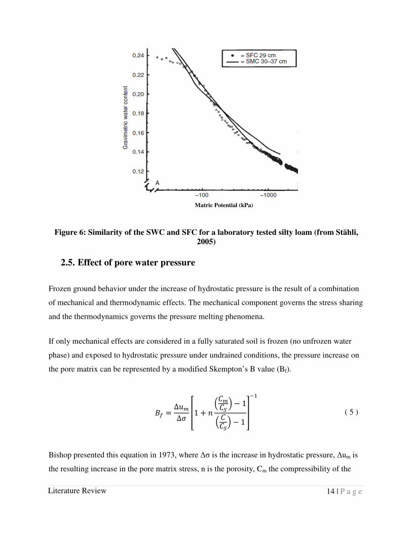
SFC for various type of soil. Figure 6 shows the similarity of both curves by superimposing on
the other.
14 | P a g e
Literature Review
Figure 6: Similarity of the SWC and SFC for a laboratory tested silty loam (from Stähli,
2005)
2.5. Effect of pore water pressure
Frozen ground behavior under the increase of hydrostatic pressure is the result of a combination
of mechanical and thermodynamic effects. The mechanical component governs the stress sharing
and the thermodynamics governs the pressure melting phenomena.
If only mechanical effects are considered in a fully saturated soil is frozen (no unfrozen water
phase) and exposed to hydrostatic pressure under undrained conditions, the pressure increase on
the pore matrix can be represented by a modified Skempton’s B value (Bf).
∆∆ 1 1
1 ( 5 )
Bishop presented this equation in 1973, where Δσ is the increase in hydrostatic pressure, Δum is
the resulting increase in the pore matrix stress, n is the porosity, Cm the compressibility of the
Gra
vim
etri
c w
ate
r co
nte
nt
Matric Potential (kPa)

15 | P a g e
Literature Review
pore matrix, CS the compressibility of the soil grains, and C the compressibility of the soil
skeleton. For saturated dense sand, nearly all pressure is transferred to the pore matrix (Ladanyi
1985).
However, when considering a three-phase material such as frozen ground with unfrozen water,
the pore water pressure increase may be much smaller. Wissa (1969) assumed that the ice would
cement the soil grains which greatly reduce the compressibility of the soil skeleton. It was found
that cement-stabilized sand would have a typical B value of 0.575 under hydrostatic pressure.
The conclusion is that a sudden increase in pressure will stress the ice more than the unfrozen
water. This increase in stress leads to thermodynamic consequences involving pressure melting
phenomena.
Figure 7: Water phase diagram (by: Christopher Auyeung)
The stress in a soil is highly concentrated at small contact points between the grains. In frozen
soils this contact area will include a layer of ice between the particles. From the water phase
diagram shown in Figure 7, water will not freeze at normal freezing temperature under high
stress. The effect is even larger when minerals are dissolved in the water.
The pressure melting phenomenon happens when the stress is high enough and/or when the
temperature changes during the test. If the stress path crosses between phases the ice will melt
16 | P a g e
Literature Review
and influence the pore water pressure. When the process is non-isothermal the relationship for
ice and water coexisting is defined by Clausius-Clapeyron equation (Hillel, 1980)
( 6 )
where γw=1000 kg/m3 is the density of water, γi=916.8 kg/m3 is the density of the ice,
L=3.336x10⁵ J/kg is the latent heat of water, dT=T0-T is the difference between normal freezing
temperature of pure water, T0=273.15 K and the actual temperature, T, of the system. The
equation becomes:
1.091 + 1.221 ( 7 )
It is important to note that u is in MPa and T in Kelvin. For the interface condition dpw=dpi=dp,
which gives the freezing-point depression for ice (Andersland, 2004).
= −0.0743 / ( 8 )
Meaning that a pressure of 13.5 MPa is needed to reduce the freezing point of water by 1°C.
Under normal condition, if it was not for grain-to-grain contact area, there would be very little
melting.
For an isothermal process, dT=0.
= 1.091 ( 9 )
From which it can be concluded that pore-water pressure follows closely the pore ice pressure as
long as there is no phase change.

17 | P a g e
Literature Review
This melting phenomenon is also a governing factor of frozen soil consolidation. Since the small
ice-particle contact area can increase the local stress by a factor of 10 to 500 compared to the
global normal pressure of the element, (Arteau, 1984) the local melting water must also migrate
to dissipate pore water pressure adding time to the process. For example, frozen sand has a
typical hydraulic gradient of approximately 10-13 m/s and a coefficient of consolidation of
10‑8 m2/s, which would require 7 months to consolidate a 100 mm long by 50 mm in diameter
test specimen. The majority of the published triaxial test results should be classified as
unconsolidated-undrained tests. An exception has to be made for specimens consolidated before
freezing (Goodman, 1975).
2.6. Rheology of soil and ice mixture
Rheology is defined as “the study of the deformation and flow of matter” in terms of stress,
strain, temperature and time (Arenson, 2015). The thermo-mechanical properties of frozen soil
are highly influenced by all four criteria. Stress and strain relates to melting pressure;
temperature modifies the amount of unfrozen water; and time is a major factor for creep,
consolidation and strength.
Figure 8: Failure mechanism map of unconfined compressive strength of frozen Ottawa
sand at -7ºC and a constant strain rate of 4.4 x 10⁻⁴
s-1
(From Andersland, 2004)

18 | P a g e
Literature Review
Ladanyi (2003) concluded that the behavior of mixture depends on the characteristics of the
constituting solid and liquid as well as their relative proportion in the mixture. Ting et al. (1983)
summarized the work and concluded that the peak strength is governed by one of three criteria
depending on the volume fraction of sand. Figure 8 shows the failure mechanism of frozen
Ottawa sand at different sand volume fraction. Ting et al.’s concluded that up to a grain volume
(Volume solids/Volume Total) fraction of 0.4, the behaviour is governed by the pore ice. For
fraction greater than 0.4 the friction resistance between the particles intervenes; and for a ratio
greater than 0.6, the dilatancy caused by interlocking of dense sand adds to shear strength.
Ladanyi (2003) approximated the results by this equation
q , q , 1 + 14.1C ) For 0<C<0.65 ( 10 )
where C is the volume fraction of sand, and qu,ice is the shear strength of pure ice.
q , = q , (1 + 14.1C ) For 0<C<0.65 ( 11 )
However, when the amount of ice decreases the cohesion decreases and eventually the strength
reverts to the one of dry soil. Figure 9 shows the effect of water content on compressive strength.

19 | P a g e
Literature Review
Figure 9: Relationship between uniaxial compressive strength of frozen sand with
temperature at different water content. (Ladanyi, 2003)
Andersland & Ladanyi (1994) presented an empirical formula to account for this effect.
q (kPa) = 15.5w(θ + 15°C) − 1373 ( 12 )
Where qu is the uniaxial compressive strength, w is the total water and ice content and θ=-T°C is
the frozen temperature of the soil.
It was found that stress-strain behaviour of frozen soil is similar to the behaviour of ice. Gold
(1970) presented the 4 responses shown in Figure 10 where ice is tested at small strain rates
(<10-5/s), response A, to higher rates (>10-2/s), response D.

20 | P a g e
Literature Review
Figure 10: Stress-strain behavior of ice under different strain rate A) ductile behavior with
strain hardening, B) dilatant behavior with strain softening, C) brittle behavior with
failure after yield point, D) brittle failure (Arenson et al., 2007)
However, the stress-strain response of a frozen soil is not only dependant on strain rate but also
depends on volumetric ice content as shown previously. Figure 11 demonstrates the response of
frozen soil to both the volumetric ice content and strain rate (Arenson & Springman, 2005).
Figure 11: Stress response of frozen ground as a function of strain rate and volumetric ice
content (Arenson et al., 2007)

21 | P a g e
Literature Review
An increase in the testing strain rate will influence the strength measured as well as the response
of the frozen sample. A low ice content soil shows a dilatant response and a high ice content soil
as a ductile response. As described by Gold (1970) and Arenson et al. (2007) a soil with high
volumetric water content will respond like pure ice.
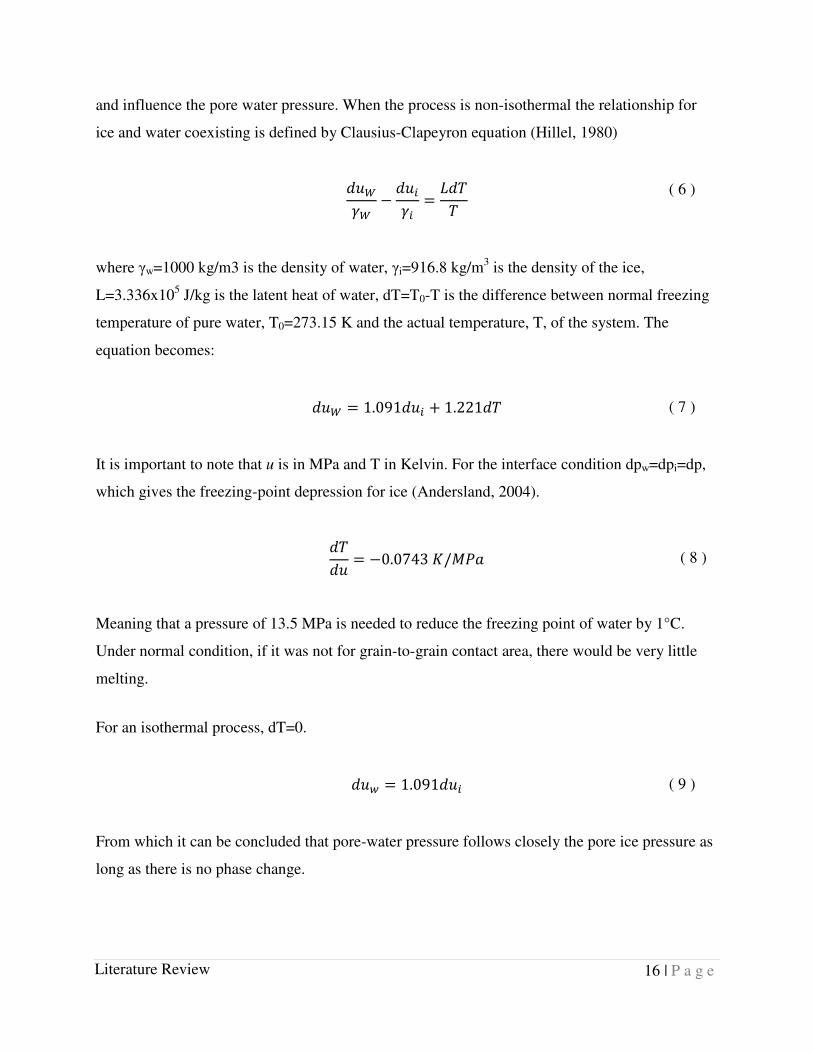
2.7. Frost Heaving
Expansion is associated with soil freezing. It is well known that freezing water will expand by
9%+. However, this 9%+ expansion doesn’t lead to a 9%+ increase in the volume of voids of the
soil. This happens as the water is being expelled from the soil during the freezing process. is due
to the water being expelled in the process.
For silty soils, the freezing process depends on the rate at which the temperature decreases (or
drops). When the freezing rate of a saturated specimen is large, the water freezes in place. If the
temperature is gradually lowered, the ice tends to accumulate in layers of clear ice parallel to the
surface exposed to the freezing temperature. As a result, frozen silty soils consist of layered ice
and soil (Andersland, 2004). For this to occur, water must migrate through the ground. The
thickness of the layers of ice depends on the freezing rate and the availability of water to the
freezing front. Figure 12(a) shows a closed system where there is no excess water available,
Figure 12(b) shows a system where there is excess water migrating towards the freezing front
and Figure 12(c) shows a system where a layer of permeable soil is blocking the water to travel
up to the freezing front.
22 | P a g e
Literature Review
Figure 12: Ice formation in soils: (a) closed system (b) open system (c) drainage layer (from
Andersland, 2004)
For in-situ freezing conditions in fine grain soils, the water would migrate from the water table
(free water layer) by capillary effect. The distance between the freezing front and the water table
has to be smaller than the height of the capillary rise of the soil. The maximum rise (hc) can be
approximated by the relationship:
ℎ 0.03
( 13 )
Where d is taken as 20% of D10.
Since the water table is continuously replenished, ice lenses can, in theory, continuously grow.
While growing, the ground above the ice layers rises. This is called frost heave, and a heave of
150 mm is not uncommon in regions that experience moderate winters (Andersland, 2004). Since
frost heave is dependent on the underlying soil profile, a coarse soil situated between the water
table and the freezing front, will negate the capillary effect and the upper zone is considered a
closed system (Figure 12 (c)).
The stress exerted from frost heave can commonly reach over 2000 kPa (Domaschuk, 1982),
giving important force to the effect of this uplift on both shallow and deep foundations. For
region susceptible to frost heave, on clay and silt consolidated deposits, foundations are installed

23 | P a g e
Literature Review
under the maximum frost front. However, for deep pile foundations the frost heave forces are
exerted directly to the structural member through the increase skin friction of adfreeze bond.
The frost heave is usually non-uniform since the permeability and shear strength of each frozen
ground is highly dependent on temperature change, permeability and water content/availability.
And so, highway structures constructed on frost sensitive soils will experience increase in
roughness and bumps. When the warmer temperature of spring thaws inter-particle ice and ice
layers, the soil becomes over saturated by water. Since the frost thaws from the top down, the
additional water will not drain until the underlying frozen soil thaws. During this time the soil is
mushy and loses most of its bearing capacity which can severely impair the pavement
(Andersland, 2004). This also gives reason to the half load condition implemented in the spring.
2.8. Adfreeze
The interface between the pile and the soil under frozen condition is commonly call adfreeze. It
has also been designated as adfreeze strength (Weaver and Morgenstern, 1981), adfreeze bond
and frozen pile-soil interface (Parameswaran, 1978) in the literature. It represents the bond
created along the surface of the pile when freezing. It has two components, adhesion due to ice
and friction due to soil grains.
Literature shows the major factors influencing adfreeze as being: ice content (Weaver and
Morgenstern, 1981), temperature (McRoberts and Nixon, 1976) and pile material (Phukan,
1978).
Data on adfreeze is important when it comes to calculating bearing capacity. This data has been
measured since the 1930's, which most of it has been derived from tests carried in the field on
undisturbed soils. (Parameswaran, 1978; Tsytovich, 1975; Vyalov, 1965). Several empirical
techniques were developed from this information.
In general, the condition presented in Equation ( 14 ) must be met for a pile installed in frozen
ground condition to support the loads.

24 | P a g e
Literature Review
> ( 14 )
The condition requires the design load (DL) and the effect of frost heave stress ( through the
pile contact area ( are counteracted by the pile end bearing capacity (P), the adfreeze strength
of the pile-soil interface , pile-frozen soil interface , friction stress between the pile and
unfrozen layer of saoil and the pile-soil interface of that layer .
Figure 13: Pile foundations bearing capacity schematic in permafrost (from
Parameswaran, 1978)
Adfreeze bearing capacity is determined at the ultimate point of rupture of the bond.
Literature shows a brittle rupture (high peak) and a small residual resistance curve after failure.
Some typical curves for different pile material are presented in Figure 14.

25 | P a g e
Literature Review
Figure 14: Adfreeze load-displacement curves for piles in frozen sand: (A) untreated B.C.
fir, (B) painted steel and (C) concrete (from Parameswaran,1978)
2.9. Ground freezing applications
Typical application of frozen ground includes access shafts, deep excavations, tunnels, ground
water control, containment of hazardous waste and a variety of special projects. Some
applications require freezing the ground. It is possible to create artificial frozen soils by installing
refrigeration pipes which cool the soil by circulating a cooling fluid in an inner tube within the
soil mass to be frozen and returning it in an outside space between two tubes (Figure 15). This
technology is frequently used to support excavations and block water flow (Figure 16).

26 | P a g e
Literature Review
Figure 15: Ground freezing tube (freeze pile) (Andersland, 2004)
The high strength, the stability and very low permeability of frozen grounds are the advantages
that engineers can exploit in their designs. The use of freezing tubes allows freezing of the
ground in any geometry. Figure 17 shows the use of these systems for tunnel and shaft
excavation. They can also be used to create impermeable walls to control water seepage and
contaminant transport.

27 | P a g e
Literature Review
Figure 16: Ground freezing tubes used to excavate (a) tunnel (Frank Coluccio
Construction, 1996) and (b) shaft (BDF, 2009)
Ground freezing is also used to obtain undisturbed cohesionless soil specimens. It is complicated
to obtain undisturbed samples of sand and gravel due to their lack of cohesion, which prevents
the soil from keeping its shape in a sampling tube. If properly frozen the sample should not be
altered by heaving. Studies have shown that if the confining pressure is maintained and drainage
is not prevented during freezing, the volume change is negligible and soil strength is not altered
upon thawing (Marcuson, 1979). To accomplish such conditions, the soil needs to be frozen at a
slow rate and be provided with a free draining boundary on the unfrozen side. Samples can then
be taken by core drilling and thawed after confining pressure has been reapplied.
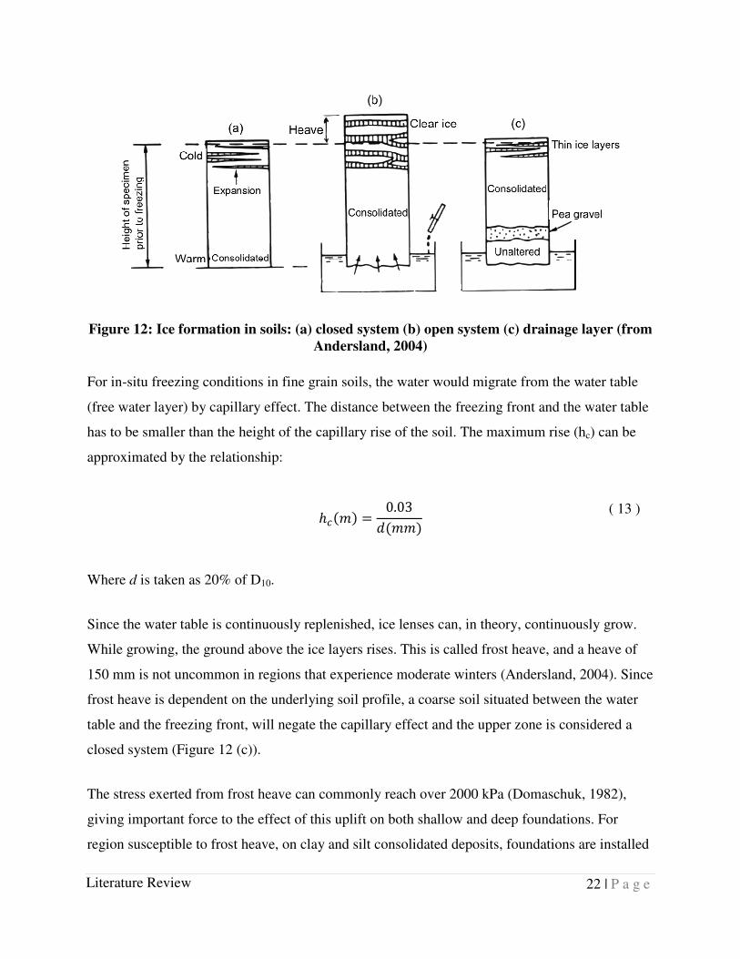
This technology can also be applied to pile foundations to ensure proper freeze bonds and
bearing capacity. However, structures commonly built on permafrost will be done so on shallow
foundations and on a non-frost susceptible soil pad with the ends of the pipe ducts exposed to air.
The ducts are open in the fall to let cold air freeze and closed during summer to limit heat
transfer. This method has proved efficient, inexpensive and easy to use.
28 | P a g e
Literature Review
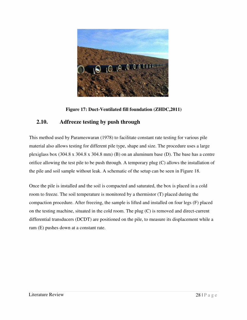
Figure 17: Duct-Ventilated fill foundation (ZHDC,2011)
2.10. Adfreeze testing by push through
This method used by Parameswaran (1978) to facilitate constant rate testing for various pile
material also allows testing for different pile type, shape and size. The procedure uses a large
plexiglass box (304.8 x 304.8 x 304.8 mm) (B) on an aluminum base (D). The base has a centre
orifice allowing the test pile to be push through. A temporary plug (C) allows the installation of
the pile and soil sample without leak. A schematic of the setup can be seen in Figure 18.
Once the pile is installed and the soil is compacted and saturated, the box is placed in a cold
room to freeze. The soil temperature is monitored by a thermistor (T) placed during the
compaction procedure. After freezing, the sample is lifted and installed on four legs (F) placed
on the testing machine, situated in the cold room. The plug (C) is removed and direct-current
differential transducers (DCDT) are positioned on the pile, to measure its displacement while a
ram (E) pushes down at a constant rate.

29 | P a g e
Literature Review
Figure 18: Schematic diagram of push through testing apparatus (Parameswaran, 1978)
The results of this study showed that two determinant factors, the type of material and roughness
of the pile, influenced its response. The different type of material and response obtained are
shown in Figure 14. Rougher and untreated surfaces show a more ductile response while
smoother surfaces and treated surfaces show a more fragile and brittle behaviour.
The study also showed the effect shear rate has on the measured adfreeze strength. Table 1
shows the peak adfreeze strength measured under different shear rate. It was also found that the
adfreeze strength (τf) follows the same power-law form as frozen soil deformation under
compression and shear which is represented by:
~ ( 15 )
where is the shear rate and m is a material constant.

30 | P a g e
Literature Review
Fragile failure indicating clean quick shearing of the interface bond was noted for all material
types at higher shear rates and not only for smoother/finer particle with lower coefficient of
friction. No testing was conducted to observe the effect of ice-poor frozen soil in the study.
Table 1: Values for peak adfreeze strength for various pile type under constant shear rate
(Parameswaran, 1978)
Cross-Head speed ( ĺ )
(mm·min-1)
Adfreeze strength (τf), MPa
B.C. fir Concrete Painted Steel
Creosoted B.C fir
Spruce Unpainted
steel Steel H-Section
0.0005 1.14 0.525 0.497 0.403 0.96 0.527 0.64
0.001 1.175 0.553 0.496 0.487 0.863 0.76 0.513
1.29
0.609
0.002 1.113 0.671 0.648 0.69 1.122 0.68 0.648
1.247
0.505
0.005 1.61 0.733 0.677 0.72 1.196 0.806 0.691
0.01 1.56 0.866 0.679 0.813 1.167 0.734 0.695
0.94
0.745
0.02 1.936 1.16 0.973 0.92 1.461 0.868 0.854
0.05 2.231 1.293 1.026 0.875 1.29 1.181 0.852
1.506
0.01 2.42 1.611 1.146 1.22 1.542 1.364 0.983
0.704
The same set up was later used to test adfreeze strength of pure ice and saline ice water on piles
for pier and bridge application (Parameswaran, 1980).
2.11. Adfreeze testing by interface shearing
Interface shearing was used by Ladanyi and Thériault (1990) to measure adfreeze strength and
observe the relationship to shear strength of the soil and the healing process of adfreeze under
creep loads.

31 | P a g e
Literature Review
A double shear apparatus was developed by Thériault (1988) which consist of 3 shear boxes
mounted on a standard shear-rate-controlled testing frame, Figure 20. The apparatus was
positioned in a cold room set at -2 ± 1°C. To maintain a better control on the temperature of the
sample, antifreeze fluid was circulated around the sample. This system was controlled by a
thermistor placed in the shear box. This allowed monitoring the temperature and controlling the
bath circulation system. The variation of temperature could then be kept below 0.1°C.
The test series included direct shear tests with sand and silt, interface shear with both soil and
steel and aluminum, and bond healing test between both soil and frozen sand or steel. All tests
were conducted at a shear rate of approximately 16.9 mm/day (0.012 mm/min).
Adfreeze bond healing is the process under which adfreeze strength is recuperated over time
under in-situ stress or normally applied load in laboratory.
The results of the study made on air free samples showed that the adfreeze bond is essentially
brittle (as shown by Parameswaran, 1978). Ladanyi and Thériault (1990) presented another
observation, the residual strength representing a small fraction of the peak strength after the
brittle failure but increases with confining load as presented in Figure 19.

32 | P a g e
Literature Review
Figure 19: Adfreeze bond of frozen sand against steel express in function of shear strength
of the frozen sand (T=-2 °C) (Ladanyi & Thériault, 1990)
As for the healing process, the adfreeze strength may only be fully recovered under relatively
high normal pressure in the order of 500 kPa. For lower normal stress the bond may only
partially heal. For fine soils like silt where the relative content of unfrozen water is higher, the
healing process was more pronounced. However, for sands, it was found that a very minimum
healing process occurred, showing that the process is favorized by the unfrozen water content
and the ability for that water to travel in the soil (Ladanyi & Thériault, 1990). For the tested silt,
the unfrozen water content was found to be 14% higher than in the tested sand.

33 | P a g e
Literature Review
Figure 20: Longitudinal cross-section of the double shear apparatus: 1. Vertical load
application; 2. Loading platen; 3. Porous stone; 4. Cylindrical bearings; 5. Antifreeze out;
6. Horizontal load application; 7. Thermistor; 8. Ball bearing; 9. Upper shear ring; 10.
Central shear ring; 11. Antifreeze in; 12. Lower shear ring (from Ladanyi and
Thériault,1990)
The study was not able to fully answer its purpose and it was suggested that larger scale testing
and observation would be needed to fully answer the concerns of adfreeze bond.
2.12. Adfreeze relation to shear strength
A considerable bank of data on adfreeze strength has been published over time. Weaver and
Morgenstern (1981) analysed the available data and related the long-term shear strength to the
adfreeze bond strength.
It was concluded that the relationship between the long term unconfined compressive strength
and the measured adfreeze bond strength can be represented by a coefficient relationship.
( 16 )

34 | P a g e
Literature Review
where τfl is the long term adfreeze, slt is the long-term shear strength of the soil and m is the
material coefficient. Table 2 shows the proposed coefficient put forward by Weaver and
Morgentstern (1981).
Table 2: Shear to adfreeze bond coefficient presented by Weaver and Morgenstern (1981)
Pile type m
Steel 0.6
Concrete 0.6
Timber (uncreosoted) 0.7
Corrugated steel pipe 1
Ladanyi and Thériault (1990) later showed that the value of m is also dependent on the normal
stress applied to the soil even if that assumption was considered negligible by Weaver and
Morgenstern (1981). Showing that the long-term pile capacity was not only dependent on long-
term adfreeze, but also depended on the residual friction angle at the interface and by correlation,
total ground lateral pressure (Aldaeef & Rayhani, 2018). Ladanyi and Thériault (1990)
ameliorated the equation by adding the contribution of the residual friction angle and presented
the following equation:
, ( 17 )
where ρh,tot is the total lateral earth pressure and Φres is the residual angle of friction.
2.13. Conclusion and direction
The available literature showed limited knowledge of frozen ground. Most practical applications
involving frozen ground relies on past experiences and field data only. The science behind the
process and effect of freezing has been studied and developed, however no major link to
practical field applications have been made.

35 | P a g e
Literature Review
When it comes to adfreeze strength and testing, useful practical data has been obtained from full
scale field test. Those tests are mostly only conducted for a specific project and can be difficult,
or impossible to generalize due to outside uncontrollable parameters such as temperature
variation, climate and soil history (Andersland, 2004).
Laboratory test data is limited since it requires special facilities (freezer chambers) and
engineering practitioners often don't see the need to test soils which in most cases are known to
perform well. Since Weaver and Morgenstern (1981) presented a relationship between shear
strength and adfreeze, it provided a quick and conservative way to account for the effect of
adfreeze.
The available adfreeze data from literature generally considers the phenomenon under air free
conditions and little is known about the effect of variable water content. This study will consider
only ice poor soil and observe the effect of modifying the water content of the specimens before
freezing.
Another discrepancy from the available research is the incompatible results obtained by different
testing methods. Even when testing similar soils, the push through method used by
Parameswaran (1978, 1980) and the interface shear method developed by Thériault (1980, 1990)
show a significant difference. This study will analyse two different methods of testing and
discuss the test results from the test series and from literature.

36 | P a g e
Model pile pull-out test
Chapter 3. Model pile pull-out test
3.1. Introduction
This chapter presents and provides the details of the first series of test conducted in this study to
measure adfreeze shaft resistance. Adfreeze strength was measured by pulling out the model pile
installed in frozen sand. The nature of the pull-out test allowed measuring only skin friction
developed at the soil-pile interface by measuring the force applied and the responding
displacement.
The objective of this phase of the study was to measure the effect of embedment depth and ice
content on adfreeze bond strength. The soil and part of the equipment used was provided by a
consultant interested in studying the adfreeze bond of typical eastern Ontario sand on piles used
to install solar panel arrays.
Freezing was achieved using outdoor temperature during the winter and in a modified freezer
during the warm seasons. Temperature was monitored using commercial USB thermistor
compatible with a Raspberry Pi computer. The key details of the equipment used during the test
program are described in this chapter. The chapter also summarize the results of the program.
3.2. Pull-out apparatus
The University of Ottawa structure laboratory is equipped with a Galdabini Sun 60 material
testing machine. This testing apparatus is equipped with a 750 000 N load cell able to test in
tension and compression. It has a 625 mm wide testing space between the load arms and a head
clearance of approximately 900 mm to permit safe testing. Figure 21shows the machine with the
installed testing setup.

37 | P a g e
Model pile pull-out test
Figure 21: Galdabini Sun 60 set up with frozen soil test box
The samples were installed in a heavy steel box 600 mm by 600 mm by 600 mm. The interior
volume of the boxes were able to accommodate 534 mm x 534 mm x 572 mm (l,w,h) specimens.
The boxes were completely sealed, impermeable, and insulated using removable foam panels on
all faces. Shop drawings are available in Appendix C.
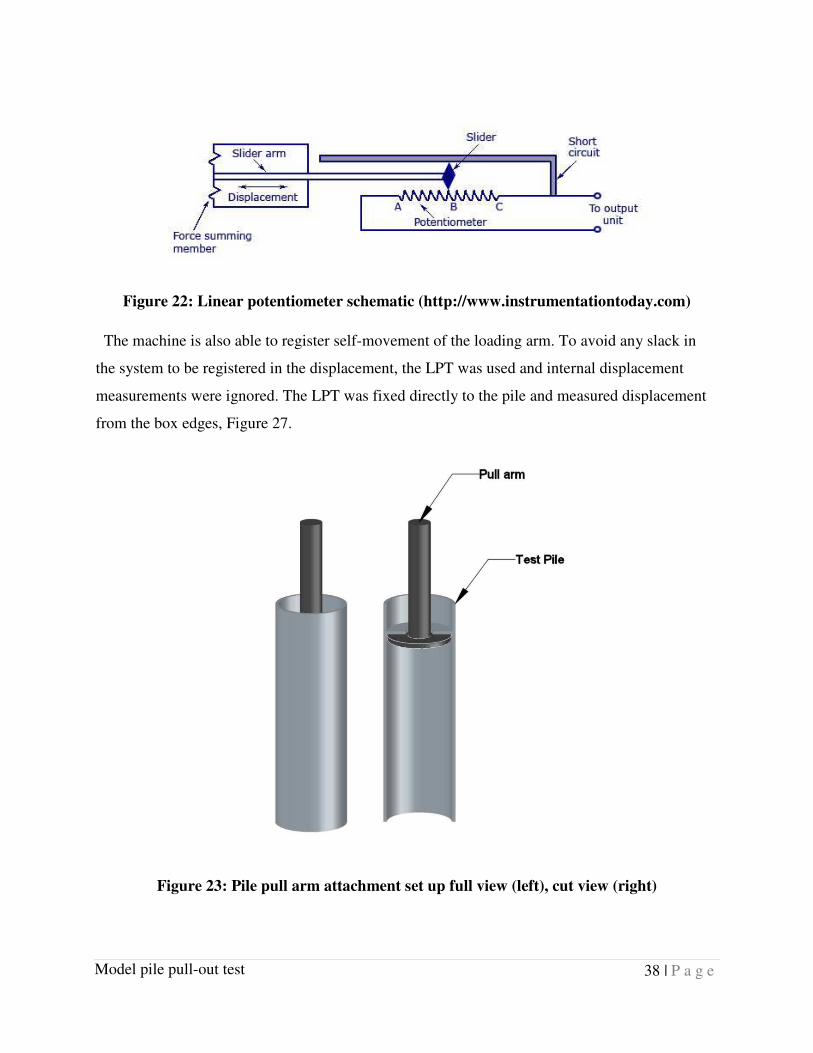
The Galdabini Sun 60 is equipped with linear potentiometer transducer (LPT) connected through
built-in serial ports. LPT measure the movement of a slider short circuiting over a potentiometer,
the movement of the sliders modifies the resistance of the circuit. The change in resistance is
calibrated to the movement of the arm, see Figure 22.
38 | P a g e
Model pile pull-out test
Figure 22: Linear potentiometer schematic (http://www.instrumentationtoday.com)
The machine is also able to register self-movement of the loading arm. To avoid any slack in
the system to be registered in the displacement, the LPT was used and internal displacement
measurements were ignored. The LPT was fixed directly to the pile and measured displacement
from the box edges, Figure 27.
Figure 23: Pile pull arm attachment set up full view (left), cut view (right)
39 | P a g e
Model pile pull-out test
The boxes were fixed to the machine by first installing a heavy 25 mm thick plate to the testing
table using four large machine bolts. The box was installed on the plate using a fork lift and
attached to the plate using eight grade 10 bolts around the perimeter HSS frame of the box. The
testing arm was then able to clamp on the pulling bar installed on top of the pile, Figure 23.
The piles provided for the program where galvanized HSS 114.3 x 8.6 lightly corrugated.
Roughness measurements are available in Chapter 4, Table 5: Roughness measurement of tested
pile and various galvanized steel plates and sheeting.
Each testing pile was outfitted with a steel plate welded directly into the hollow core. A hole was
drilled in the plate to insert a puling bar. The bars were approximately 19 mm in diameter.
Another plate was welded at one end of the rod. When inserted in the pile the two plates would
transfer the load to the pile. Figure 23 shows the pile attachment. More drawings are available in
appendix C describing the box and attachment to the testing machine.
3.3. Tested soil properties
The soil provided for testing was taken from a potential solar panel field located in proximity to
Cornwall, Ontario (Canada). The soil composed the surface layer of the site. The received soil
had an average gravimetric moisture content of 12%. A series of standard test was conducted to
classify the soil.
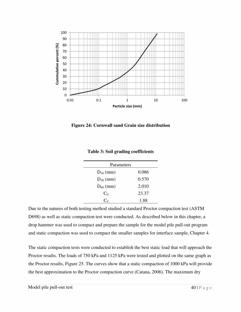
The results of a sieve analysis are presented in Figure 24 and the results for the coefficient of
uniformity (Cu) and the coefficient of curvature (Cc) are presented in Table 3. According the
unified soil classification system (USCS) the soil can be classified as well graded sand (SW).
40 | P a g e
Model pile pull-out test
Figure 24: Cornwall sand Grain size distribution
Table 3: Soil grading coefficients
Parameters
D10 (mm) 0.086
D30 (mm) 0.570
D60 (mm) 2.010
CU 23.37
CC 1.88
Due to the natures of both testing method studied a standard Proctor compaction test (ASTM
D698) as well as static compaction test were conducted. As described below in this chapter, a
drop hammer was used to compact and prepare the sample for the model pile pull-out program
and static compaction was used to compact the smaller samples for interface sample, Chapter 4.
The static compaction tests were conducted to establish the best static load that will approach the
Proctor results. The loads of 750 kPa and 1125 kPa were tested and plotted on the same graph as
the Proctor results, Figure 25. The curves show that a static compaction of 1000 kPa will provide
the best approximation to the Proctor compaction curve (Catana, 2006). The maximum dry
0
10
20
30
40
50
60
70
80
90
100
0.01 0.1 1 10 100
Cu
mm
ula
tiv
e p
erc
en
t (%
)
Particle size (mm)

41 | P a g e
Model pile pull-out test
density and optimum water content from the Proctor test was 2026 kg/m3 and 11.6 %
respectively.
A standard specific gravity test (ASTM D7263) provided a value of 2.65.
Figure 25: Proctor and static compaction curve
3.4. Sample preparation
The empty steel box was first filled with a 50 mm thick compacted layer of the same soil to be
tested. The purpose of this bottom layer is to avoid any steel on steel bond to be created or ice
accumulation bonding the bottom of the pile. This step was added following the first test
conducted at full depth of the box. The pile was then inserted, centred and levelled using four
temporary wooden struts.
The maximum embedment depth that the setup allowed to test was 572 mm, however at that
depth the pile was resting on the metal bottom of the box and the forces damaged part of the
equipment. The tests were then conducted avoiding metal on metal contact and at depth starting
at 521 mm with the exception of a test at 533 mm which rested directly on the bottom of the test
box.
1700
1750
1800
1850
1900
1950
2000
2050
2100
8 9 10 11 12 13 14 15 16
Dry
de
nsi
ty (
kg
/m3)
Gravimetrique water content (%)
Standard Proctor
750 kPa Static
1250 kPa Static

42 | P a g e
Model pile pull-out test
The sand was then mixed with water to achieve predetermined water content and compacted in
lifts of 50 mm with a custom drop hammer to approach the proctor curve as much as possible.
The process was repeated until the desired sand thickness was achieved. The struts were
removed when the sand could support the pile. Density was measured after the test was
completed to avoid disturbance. The standard test method for density and unit weight of soil in
place by the rubber balloon method (ASTM D2167) was used to obtain the average density of
the sample.
Temperature could be monitored in real time using waterproof USB DS18B20 thermistor by
Adafruit. The sensors have an accuracy of ±0.5 °C from -10 °C to 85 °C.
Figure 26: Waterproof DS18B20 Digital temperature sensor (Adafruit)
Three USB thermistors were inserted between the centre lifts 25 mm from the pile, in the center
of the pile and the box’s wall and 25 mm from the wall. A fourth sensor was inserted in the
center of the pile and the box’s wall before the last lift. Those thermistors allowed real-time
monitoring of the sample temperature during testing.
The samples were frozen in an extended upright household freezer during summer and outside
during winter time. The temperature inside the freezer reached -8 °C. Exterior temperature
during January and February 2015 was on average -22 °C. The sample was tested while internal
temperature was lower than -5 °C.
43 | P a g e
Model pile pull-out test
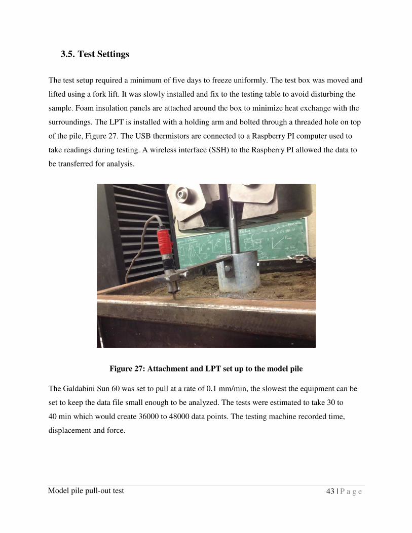
3.5. Test Settings
The test setup required a minimum of five days to freeze uniformly. The test box was moved and
lifted using a fork lift. It was slowly installed and fix to the testing table to avoid disturbing the
sample. Foam insulation panels are attached around the box to minimize heat exchange with the
surroundings. The LPT is installed with a holding arm and bolted through a threaded hole on top
of the pile, Figure 27. The USB thermistors are connected to a Raspberry PI computer used to
take readings during testing. A wireless interface (SSH) to the Raspberry PI allowed the data to
be transferred for analysis.
Figure 27: Attachment and LPT set up to the model pile
The Galdabini Sun 60 was set to pull at a rate of 0.1 mm/min, the slowest the equipment can be
set to keep the data file small enough to be analyzed. The tests were estimated to take 30 to
40 min which would create 36000 to 48000 data points. The testing machine recorded time,
displacement and force.
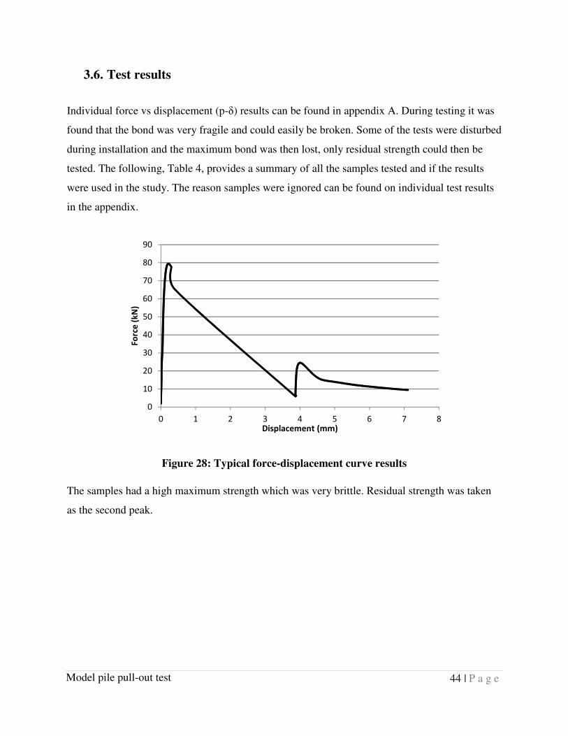
44 | P a g e
Model pile pull-out test
3.6. Test results
Individual force vs displacement (p-δ) results can be found in appendix A. During testing it was
found that the bond was very fragile and could easily be broken. Some of the tests were disturbed
during installation and the maximum bond was then lost, only residual strength could then be
tested. The following, Table 4, provides a summary of all the samples tested and if the results
were used in the study. The reason samples were ignored can be found on individual test results
in the appendix.
Figure 28: Typical force-displacement curve results
The samples had a high maximum strength which was very brittle. Residual strength was taken
as the second peak.
0
10
20
30
40
50
60
70
80
90
0 1 2 3 4 5 6 7 8
Fo
rce
(k
N)
Displacement (mm)
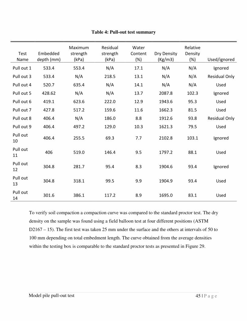
45 | P a g e
Model pile pull-out test
Table 4: Pull-out test summary
Test
Name
Embedded
depth (mm)
Maximum
strength
(kPa)
Residual
strength
(kPa)
Water
Content
(%)
Dry Density
(Kg/m3)
Relative
Density
(%) Used/ignored
Pull out 1 533.4 553.4 N/A 17.1 N/A N/A Ignored
Pull out 3 533.4 N/A 218.5 13.1 N/A N/A Residual Only
Pull out 4 520.7 635.4 N/A 14.1 N/A N/A Used
Pull out 5 428.62 N/A N/A 13.7 2087.8 102.3 Ignored
Pull out 6 419.1 623.6 222.0 12.9 1943.6 95.3 Used
Pull out 7 427.8 517.2 159.6 11.6 1662.3 81.5 Used
Pull out 8 406.4 N/A 186.0 8.8 1912.6 93.8 Residual Only
Pull out 9 406.4 497.2 129.0 10.3 1621.3 79.5 Used
Pull out
10 406.4 255.5 69.3 7.7 2102.8 103.1 Ignored
Pull out
11 406 519.0 146.4 9.5 1797.2 88.1 Used
Pull out
12 304.8 281.7 95.4 8.3 1904.6 93.4 Ignored
Pull out
13 304.8 318.1 99.5 9.9 1904.9 93.4 Used
Pull out
14 301.6 386.1 117.2 8.9 1695.0 83.1 Used
To verify soil compaction a compaction curve was compared to the standard proctor test. The dry
density on the sample was found using a field balloon test at four different positions (ASTM
D2167 – 15). The first test was taken 25 mm under the surface and the others at intervals of 50 to
100 mm depending on total embedment length. The curve obtained from the average densities
within the testing box is comparable to the standard proctor tests as presented in Figure 29.
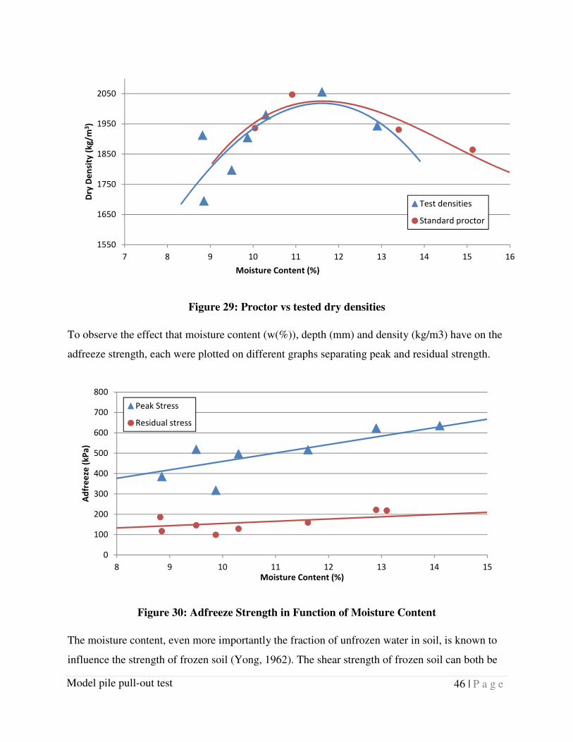
46 | P a g e
Model pile pull-out test
Figure 29: Proctor vs tested dry densities
To observe the effect that moisture content (w(%)), depth (mm) and density (kg/m3) have on the
adfreeze strength, each were plotted on different graphs separating peak and residual strength.
Figure 30: Adfreeze Strength in Function of Moisture Content
The moisture content, even more importantly the fraction of unfrozen water in soil, is known to
influence the strength of frozen soil (Yong, 1962). The shear strength of frozen soil can both be
1550
1650
1750
1850
1950
2050
7 8 9 10 11 12 13 14 15 16
Dry
De
nsi
ty (
kg
/m3)
Moisture Content (%)
Test densities
Standard proctor
0
100
200
300
400
500
600
700
800
8 9 10 11 12 13 14 15
Ad
fre
eze
(k
Pa
)
Moisture Content (%)
Peak Stress
Residual stress

47 | P a g e
Model pile pull-out test
reduced and increased by raising the water content of the soil. The strength increases until the
soil is saturated once the saturation content is passed the sample will then lose strength by
increasing its water content. When the volumetric water content is increased passed a threshold
value of 10% (Arenson, 2007) the water act more like “Dirty Ice”.
Dirty ice acts very closely to pure ice; it represents water with a volume fraction of soil below
0.5. The relationship and effect of volume ratio is presented on Figure 8.
Figure 30: Adfreeze Strength in Function of Moisture Content, shows the curve approaching full
saturation. The degree of saturation for the compaction used for testing was found to be between
16 and 17%. As described by Weaver and Morgenstern (1981) the relationship between shear
strength of the frozen soil and its adfreeze coefficient is proportional. It is then expected that
over saturated soil samples will demonstrate the same behaviour under adfreeze testing.
Figure 31: Adfreeze strength in function of density
Figure 31 shows that density has little effect on bond strength. The majority of the bond strength
gained by freezing comes from the ice (Aldaeef & Rayhani, 2018). Unfrozen water form
penetrates between the steel and the soil as well as all the imperfection in the materials. When
freezing, water expands and cements the interface (Wissa, 1965) between soil particles and the
pile material. This cementing effect increases the interface bond in some conditions up to 10
0
100
200
300
400
500
600
700
1650 1700 1750 1800 1850 1900 1950 2000 2050 2100
Ad
fre
eze
(k
Pa
)
Dry Density (kg/m3)
Peak Stress
Residual Stress

48 | P a g e
Model pile pull-out test
times the thawed bond. Even if the particles are closer the interlocking effect is not significantly
increased since most of the load is transferred through the ice (Ladanyi 1985).
Figure 32: Adfreeze strength in function of embedded depth
3.7. Observations
3.7.1. Fragile bond
During the testing procedures it was found that the bond is fragile. The sample loses its peak
maximum adfreeze bond if it had been exposed to vibration or a shock. On two occasions the
forklift used to install the sample on the testing machine was holding the box too high and the
pile came in contact the machine’s arm. The unquantifiable shock seemed to be insignificant at
the time the lateral load was applied. From the adfreeze peak strength, however, it was found that
displacements on the order of 0.5 mm were sufficient to break the bond. The piles reached their
maximum capacity between 0.3 and 0.6 mm of displacement.
Pull-out tests 3 and 8 shown in appendix present the results of the disturbed samples. This level
of sensitivity is due to the shallow embedment depth. The lateral resistance of these small piles is
small especially for the small displacement needed to break the adfreeze maximum bond.
0
100
200
300
400
500
600
700
800
0 100 200 300 400 500 600
Ad
fre
eze
(k
Pa
)
Depth (mm)
Peak Stress
Residual Stress

49 | P a g e
Model pile pull-out test
3.7.2. Effective bond depth
The lateral pressure was assumed to be negligible around the tested piles due to the shallow
absolute depth of their embedment. Figure 6 show the soil separating from the surface of the pile.
The extent of the effect could not be measured and was not visible for all piles. The lower the
water content of the soil the more visible the crack was. The same trend was observed for
shallow embedment depth: the shallower the pile embedment, the larger the crack that would be
formed.
The effect for small diameter-shallow piles might be important in affecting the capacity of the
pile. Different experiments should be done to establish if there is an effective depth to be used in
calculating capacity of piles in frozen ground. The installation method and type soil may also
influence this behaviour.
Figure 33: Soil interface separation at the surface of the sample

50 | P a g e
Soil Interface Testing
Chapter 4. Soil Interface Testing
4.1. Introduction
This chapter presents the equipment and method used to test adfreeze bond using a direct shear
interface apparatus. The apparatus was modified and outfitted with refrigeration equipment to
enable in place tests at freezing temperatures. First, surface testing was conducted to ensure the
interface tested was of similar roughness as the model pile tested in Chapter 3. Secondly a range
of normal stress was chosen for testing from the literature review. Finally, compaction and
preparation of the sample was done to approach the same conditions tested in Chapter 3.
The results and observation are presented following the testing procedure. The objective of this
part of the experimental program is to measure adfreeze bond using a small size sample in a soil-
interface testing apparatus like apparatuses found in practical testing laboratories.
4.2. Soil-Interface apparatus
In frozen ground it is a common practice to consider the soil-pile interface as the only load
transfer mechanism (Ladanyi and Theriault, 1990). By doing so, the end-bearing capacity is
ignored, and the system is simplified to the material and soil interface. For axially loaded
elements such as piles the system can be represented by a flat surface of the pile material in
contact with soil under a normal force.
An automated three-dimensional interface testing apparatus was developed and presented by
Fakharian and Evgin in 1996 at the University of Ottawa. This apparatus can be programed and
modified easily for a range of interface testing. A schematic of the machine is presented in
Figure 34. Its small size and testing enclosure made it easy to convert into a cold room using
insulation panels and refrigeration equipment. It makes this apparatus one of the first to freeze
and test samples without require handling the specimen after freezing.
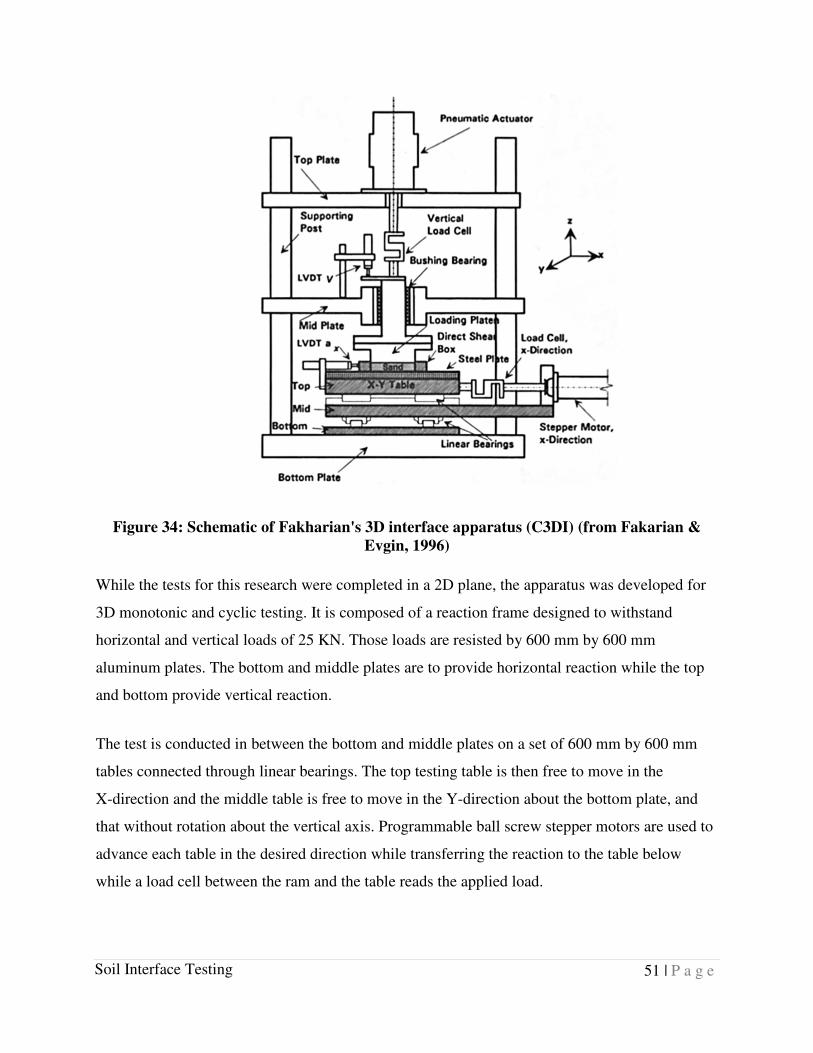
51 | P a g e
Soil Interface Testing
Figure 34: Schematic of Fakharian's 3D interface apparatus (C3DI) (from Fakarian &
Evgin, 1996)
While the tests for this research were completed in a 2D plane, the apparatus was developed for
3D monotonic and cyclic testing. It is composed of a reaction frame designed to withstand
horizontal and vertical loads of 25 KN. Those loads are resisted by 600 mm by 600 mm
aluminum plates. The bottom and middle plates are to provide horizontal reaction while the top
and bottom provide vertical reaction.
The test is conducted in between the bottom and middle plates on a set of 600 mm by 600 mm
tables connected through linear bearings. The top testing table is then free to move in the
X-direction and the middle table is free to move in the Y-direction about the bottom plate, and
that without rotation about the vertical axis. Programmable ball screw stepper motors are used to
advance each table in the desired direction while transferring the reaction to the table below
while a load cell between the ram and the table reads the applied load.

52 | P a g e
Soil Interface Testing
Figure 35: Foam insulation panel covering the testing chamber of the C3DI
The normal load is applied by a pneumatic actuator from the acting from the top of the frame. It
applies a load in the Z axis through vertically mounted bushing bearing fixed against X-Y plane
movement. The load is then applied through a loading plate that fits in the 100 mm by 100 mm
direct shear box in which the soil sample is prepared. An LPT is fixed to the middle plate to
measure normal displacement of the specimen. (for more details, Fakharian & Evgin (1996))
To adjust the apparatus for freezing interface tests, the testing chamber between the bottom and
middle plates was fully enclosed within insulation foam panels, as shown in Figure 35. The
inside view of the testing table and normal load plate is shown in Figure 36. The figure also
shows tubes, which can be use to circulate a fluid through the testing table for gradient
temperature testing, however, those were not used for this series of tests, as the tubes were
disconnected, and the interface plate was thus subjected only to the temperature of the insulated
chamber. The bolted plates were used to hold the sample and shear box in place for preparation
and installation. The LPT seen in the foreground was used to measure displacement in the X
axis. The load cell on the right leads to the Y axis stepper motor not used for these tests. The X
axis set up is the same on the far side of the table.

53 | P a g e
Soil Interface Testing
Figure 36: Interface testing table inside the insulated chamber
4.3. Freezing equipment
The testing chamber was refrigerated by 2 electrical refrigeration box panel able to cool air down
by 20°C from the ambient temperature and 2 vortex tubes which injected air between -7 and
-6°C in the chamber. This system was able to freeze and keep the testing table at a temperature
of -4 ± 0.5°C. Being able to freeze the specimen within the testing enclosure protects the fragile
adfreeze bond from potential disturbance during transportation.
4.3.1. Refrigeration panels
The refrigeration panels used were taken off an Igloo Iceless Thermoelectric Cooler, Figure 37.
The panel is specified to refrigerate and keep the temperature of the cooler box 20°C below
ambient temperature. Two panels were glue and seal to the foam insulation around the testing
chamber allowing proper ventilation for the refrigeration system. Using this system allowed to
stabilize and avoid temperature fluctuation in the chamber. They were not the main source of
cooling.

54 | P a g e
Soil Interface Testing
Figure 37: Colling equipment: Igloo Iceless Thermoelectric Cooler (left) (Terapeak.com),
Exair vortex tube (rigth) (exair.com)
4.3.2. Vortex tubes
Vortex tubes are a reliable, low cost and maintenance free solution for cooling small areas. They
require only a steady flow of compress air to operate. As shown in Figure 38, the input
compressed air is separated in two different streams of different temperature. The apparatus uses
a vortex to split the denser colder air particles from the warmer lighter air. The Exair Model 3210
vortex tube can output a temperature range from -46°C to 127°C depending on the temperature,
pressure and flow rate of the feed compressor. The preferred temperature can be set using the
adjustable valve on the warm outflow side of the tube.
Two Exair Model 3210 vortex tubes were installed to push freezing air in the testing chamber.
The laboratory is equipped with compressed air lines able to provide the required flow of 4.8 l/s
at 6.9 Bar of pressure for the proper function of the vortex. The tubes were set to provide a
continuous flow of air at a temperature of -7°C.
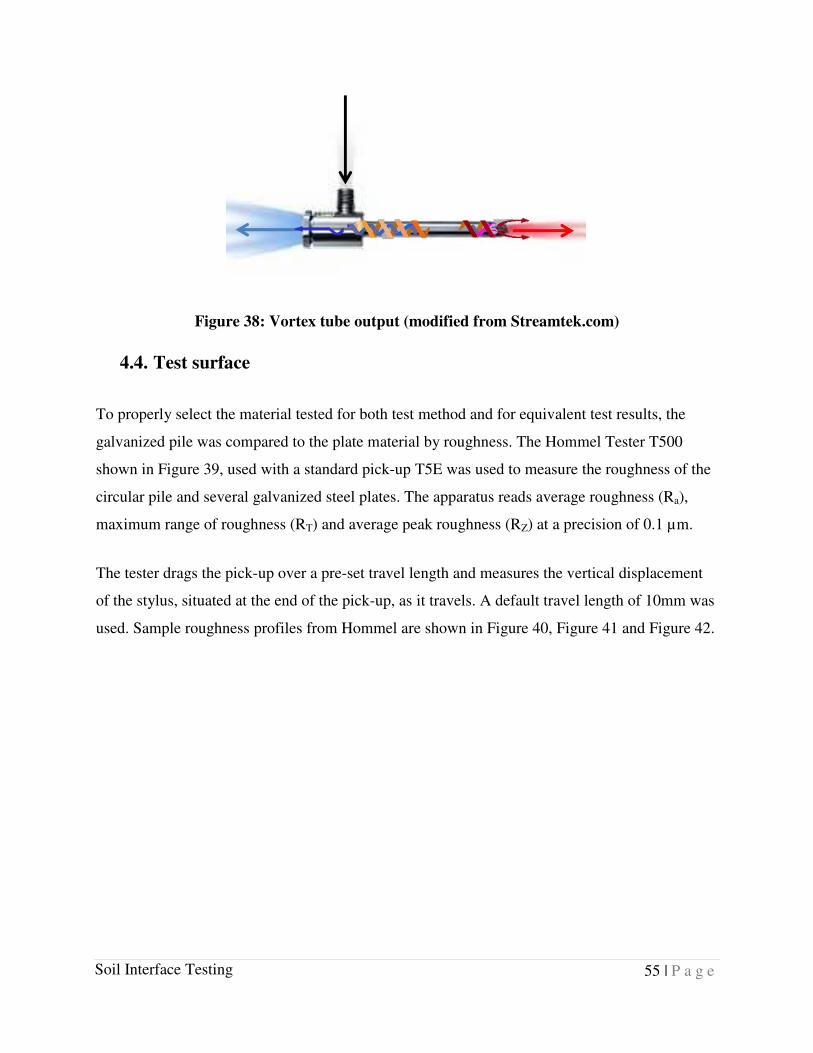
55 | P a g e
Soil Interface Testing
Figure 38: Vortex tube output (modified from Streamtek.com)
4.4. Test surface
To properly select the material tested for both test method and for equivalent test results, the
galvanized pile was compared to the plate material by roughness. The Hommel Tester T500
shown in Figure 39, used with a standard pick-up T5E was used to measure the roughness of the
circular pile and several galvanized steel plates. The apparatus reads average roughness (Ra),
maximum range of roughness (RT) and average peak roughness (RZ) at a precision of 0.1 µm.
The tester drags the pick-up over a pre-set travel length and measures the vertical displacement
of the stylus, situated at the end of the pick-up, as it travels. A default travel length of 10mm was
used. Sample roughness profiles from Hommel are shown in Figure 40, Figure 41 and Figure 42.

56 | P a g e
Soil Interface Testing
Figure 39: Hommel tester T500 Roughness meter (http://granat-e.ru/t500)
Ra is defined by the arithmetic mean of the profile deviation from the center line over the
measuring length (lm). Graphically, it is the area between the roughness profile and its center
line, Figure 40. It is calculated by integrating the displacement of the stylus over the travel
length, Equation ( 18 ).
| | ( 18 )
Figure 40: Roughness profile with average roughness (Hommel)
RT representes the maximum vertical displacement of the stylus over the travel length. It is
defined by measuring the maximum peak value (RP) and the lowest valley value (RV) peak of the
graphical representation and adding them together, Figure 41.

57 | P a g e
Soil Interface Testing
( 19 )
Figure 41: Roughness profile with maximum roughness (Hommel)
RZ is taken as the mean of the absolute value of the five (5) highest peak (YP) and five (5) lowest
valleys (YV). It represents the average maximum displacement of the stylus over the travel
length.
15 | | | | ( 20 )
Figure 42: Roughness profile with average peak roughness (Hommel)
A variety of galvanized steel plate and sheeting were tested to find the best match to the surface
of the piles tested in the pull-out series of tests. The results of the measurements are presented in
Table 5. The measurements were done at multiple locations and directions on the surface of the
pile and plating. The best comparable sheeting material available was the corrugated galvanized
sheeting 1. Two sheets of the material were cut and fitted to the testing table of the apparatus for
testing.

58 | P a g e
Soil Interface Testing
Table 5: Roughness measurement of tested pile and various galvanized steel plates and
sheeting
Pull-Out test pile
Rz (μm) 4.76 7.66 8.76 7.9 19 14.48 8.64
Ra (μm) 0.6 0.96 1.7 1.5 4 2.52 1.26
RT (μm) 6.06 10.26 11.14 9.24 23 17.22 12.6
Galvanized plate corrugated 1
Rz (μm) 23.76 17.78 16.76 18.6
Ra (μm) 3.74 2.5 2.66 2.5
RT (μm) 31.22 23.3 18.9 28
Galvanized plate corrugated 2
Rz (μm) 36.8 31.7 34.1 34.2
Ra (μm) 8.6 5.7 5.4 5
RT (μm) 43.5 32.7 44.7 43.8
Galvanized sheeting 1
Rz (μm) 1.94 1.62 3.22 2.44
Ra (μm) 0.34 0.24 0.58 0.44
RT (μm) 2.42 2.28 4.26 3.04
Galvanized sheeting corrugated 1
Rz (μm) 9.3 8.92 10.04
Ra (μm) 1.34 1.28 1.44
RT (μm) 12.04 11.68 12.6
4.5. Sample Preparation
The interface apparatus was developed to test 100 mm by 100 mm samples with a maximum
thickness of 23 mm. The sample is prepared in an aluminum direct shear box 25 mm thick with a
100 mm square opening. The underside of the box is lined with a Teflon layer to minimize
friction and prevent sand from leaking under. The shear box is shown in Figure 43 during the
preparation of a sample.
To prepare the sample, the shear box is first installed on the testing table and centered down with
the vertical load ram. Once in place the box is fixed to the table using the available clamps

59 | P a g e
Soil Interface Testing
attached to the table. The top part of the table is then removed from the machine for proper
handling and access.
Figure 43: Shear box with Teflon layer (left); Sample being compacted in load frame with
proving ring(centre); Sample after compaction (right)
A dry sample of soil is then manually mixed with the calculated amount of water to achieve the
target gravimetric water content for the specific test. The box is then filled with the well mixed
soil and levelled out. To reach the maximum dry density achieved from the standard Proctor test,
the box is put in a loading frame where it is compacted under static load using a ram, a jack and a
calibrated proving ring to monitor the load. See Figure 25 for compaction test, the sample are
compacted at 1000 kPa before being removed from the loading frame. To be properly prepared
the sample needs to be approximately 5 mm from the top of the shear box after compaction. If
the sample is found to be too thin or not leveled after compaction, more soil is added and the
re-compacted.
A plastic wrap film is put over the sample to avoid the soil freeze-bonding to the load ram during
the freezing. The table is reinserted in the testing chamber and fixed in place. The chamber is
already at the target temperature.
The load ram is lowered on the sample and the target normal load is applied using the manual
configuration of the pneumatic actuator. The clamps holding the shear box are removed since the

60 | P a g e
Soil Interface Testing
ram is now holding the setup in place. The X-Axis LPT is then replace and adjusted to be ready
for testing.
The foam panel is put back in place and the sample was left to freeze for 30hrs. A thermometer is
inserted through one of the insulating panels to monitor the temperature in the chamber with an
accuracy of 0.5 °C.
4.6. Test Settings
Once the sample is ready and frozen for testing, a computer running a Benchmate™ based
software will automatically control the test. The system comprises the testing apparatus and
transducers, interface unit (hardware), and the software itself. The software can control; the
normal load through automatic commands to the actuator; the push/pull rate of the stepper motor,
as well as monitoring the displacement and loads on the sample in all directions. The output
provided is a comma separated data file (.csv) providing the readings of all transducers (LPTs
and load cells) every 5 seconds for the duration of the entire testing procedure.
The step motor controlled the shearing for this set up to push or pull the table while testing. For
one test the table is pushed by the stepper motor while for the other, the table is pulled. This is
done so that the motor stays within its working range while allowing enough movement for the
test. The testing range of the motor is approximately 14 ± 1 mm. This range is the maximum
movement that the table can accommodate without reaching the limit of the linear bearings. The
program was set to allow a maximum movement of 7 mm in either direction during the tests.
For this research the parameters that varied were the normal load and the water content of the
sample. The chamber temperature and the strain rate were kept constant through the entire
testing series. The sample water contents were 9, 11 and 13% and each were tested under normal
loads of 350, 400 and 450 kPa. The temperature of the chamber was kept at -4 ± 0.5°C. The
stepper motor was set to strain the sample at a rate of 0.1 mm/min.

61 | P a g e
Soil Interface Testing
The software requires a maximum displacement for each test. By default, the value is set at
5 mm for either direction. For the current tests, the value was set to 7 mm which is the maximum
the software allows for each testing sequence.
After the test was completed the specimen was removed and a sample was taken to measure the
water content.
4.7. Test results
For this research three normal stress values were used. Since the apparatus maximum capacity is
set to be 500 kPa the testing stresses selected were 350, 400 and 450 kPa. Five tests were
completed for each normal stress. The moisture content used to test was 9, 11 and 13%. Some
tests were doubled when the results or curve obtained deviated from previous tests. More
importance was given to the 11% moisture content due to it being the optimum water content of
the soil.
Some issues arose for the 13% moisture content specimens. The sample at this water content
could not retain all its water which would then seep out from under the shear box. This, in turn,
resulted in the shear box becoming cemented to the testing table, falsifying the test results.
Consolidation of the sample is required in future test series.
Individual test results and curves are available in appendix. A summary table is presented under
Table 6. Maximum peak adfreeze bond stress, residual strength and moisture content of each test
is indicated and classified by normal pressure. The name of each test follows this format:
“normal stress (kPa)”, “F (frozen)”, “moisture content (%)”, “Alphabetical counter”. For
example, a test conducted under 350 kPa of normal stress with 11% moisture content which is
the third repetition is indicated by “350F11C”. In preparation for testing multiple specimens,
dummy tests were conducted to calibrate and test the apparatus. Some tests were completed in
the frozen state while others were conducted under room temperature using the tested soil or a
dummy block. The dummy block was a steel block placed in the shear box which allowed the
calibrating the machine by simulating a test sequence.

62 | P a g e
Soil Interface Testing
Table 6: Interface shear test results
Name 350F09A 350F09B 350F09I 350F11I 350F13I
Normal Stress (kPa) 350 350 350 350 350
Peak Strength (kPa) 175.6 190.5 296.3 450.8 143
Residual Strength (kPa) N/A N/A 111.2 120 N/A
Moisture content (%) 9 9 9 11 13
Name 400F09A 400F11A 400F11I 400F11J 400F11K
Normal Stress (kPa) 400 400 400 400 400
Peak Strength (kPa) 246.8 177.6 52.9 195.2 185.1
Residual Strength (kPa) N/A N/A 29.8 105.1 N/A
Moisture content (%) 9 11 11 11 11
Name 450F09A 450F11A 450F11I 450F11M 450F13A
Normal Stress (kPa) 450 450 450 450 450
Peak Strength (kPa) 286.1 237.3 294.9 229.8 154.6
Residual Strength (kPa) N/A N/A 219.7 127.5 N/A
Moisture content (%) 9 11 11 11 13
A series of test on frozen specimens with 7% water content was done as preliminary testing.
Those tests did not use the same normal stresses chosen for the testing program. However, those
results were found to be worth indicating since the trend found was comparable to the one
obtained during the pull-out program. Table 6 shows those preliminary test results.

63 | P a g e
Soil Interface Testing
Table 7: Preliminary interface test series results
Name 100JF07A 150JF07A 300JF07A 300JF07B 450JF07A
Normal Stress (kPa) 100 150 300 300 450
Peak Strength (kPa) 67.1 103 183 168.8 238.6
Residual Strength (kPa) N/A N/A N/A N/A N/A
Moisture content (%) 7 7 7 7 7
Since all samples were compacted under the same normal stress, only 2 curves were made from
the data generated. Figure 44 shows the relationship obtained between the adfreeze strength and
moisture content of the samples under each normal pressure.
Figure 44: Interface testing relationship between moisture content and adfreeze stress in
function of normal stress
No observable trend could be identified in relation to moisture content due to water seeping out
of the sample during the freezing process.
0
50
100
150
200
250
300
350
400
450
500
6 7 8 9 10 11 12 13 14
Ad
fre
ee
Str
ess
(k
Pa
)
Moisture Content (%)
100 kPa
150 kPa
300 kPa
350 kPa
400 kPa
450 kPa

64 | P a g e
Soil Interface Testing
The second data arrangement is shown in Figure 45. It graphically represents the relationship
between normal stress and maximum adfreeze shear stress in function moisture content of the
specimen.
Figure 45: Interface testing relationship between normal stress and adfreeze stress in
function of sample moisture content
Ignoring the outliers, it is possible to observe 4 distinctive linear trends. In this case each curve is
separated by 5º and tends towards 0.
4.8. Observations
4.8.1. Reproducibility
The limited results from the series of test conducted shows that the machine is consistent and that
the results obtained can be reproduced. The cluster of results tested at 400 kPa with 11% water
content is a good indication that each test was completed in the same way and reacted in the
same way. It is to note that some outliers are also present and could not be explained.
0
50
100
150
200
250
300
350
400
450
500
50 150 250 350 450 550
Ad
fre
eze
Str
ess
(k
Pa
)
Normal Stress (kPa)
7%
9%
11%
13%

65 | P a g e
Soil Interface Testing
4.8.2. Moisture seepage and sample consolidation
During the 13% water content testing phase, water was observed seeping down and out of the
sample. This free water would not seep immediately and be observable before installing the
testing plate in the apparatus. This slow process would let water under the shear box which
would freeze in place and bind the box to the testing plate.
The tested values for those tests were lower than to previously obtained results of the pull-out
test series. On closer inspection, the water did not just seep out of the soil sample but also
accumulated at the bottom of the soil boundary and under the shear box. Parameswaran (1978),
Weaver and Morgenstern (1981), Crory (1966) and Andersland (2004) indicated that shear
strength of frozen soil is inversely proportional to ice content. This indicates that adfreeze
strength tends towards the adfreeze strength of pure ice only, which according to Saeki (2011)
ranges from 50 kPa to 100 kPa approximately for the shear rate and normal pressure used during
these tests. The added bond did not increase the strength of the system but reduced it.
The concentrated high moisture content layer that was observed in some of the 11% tests and all
the 13% tests, diminish the actual adfreeze strength expected for those samples. It also shows
that the lower level of the sample is over saturated.
For water contents lower than the optimum water content, the suction of the dry soil is able to
retain the water between the particles during the small consolidation time before the water
freezes.
4.8.3. Boundary effect
It is well known that the direct shear apparatus induces stress concentration in samples. This
apparatus is already known to cause stress concentration from the applied normal load if the
sample is not perfectly levelled after compaction. (Fakharian & Evgin, 1996)
It was also observed, as shown in Figure 46, that the boundary also deforms the sample. The
shear box is held in placed by the vertical loading ram while the sample is frozen to the testing
table as well as the shear box side. However, the frozen samples are much stiffer than room

66 | P a g e
Soil Interface Testing
temperature samples. The adfreeze bond itself is approximately 60 to 70% of the shear strength
of the sample according to Weaver & Morgenstern (1981). This force can deform the edge of the
sample.
As shown in Figure 46 the deformation is maximum at the centre of the edge boundary were the
other boundaries are not influencing the sample. The extent of the border effect on the result is
unknown and is difficult to control. Some specimens were observed to have larger deformations,
and some did not show an effect of the edge.
This effect is an indication of the shear for of the sample but also indicates stress concentration
in corners and along the opposite edge. This stress concentration would fail the adfreeze locally
and diminish the global observed strength. It is probably the reason the results and curves
resemble more the residual data found in the literature and observed previously in the pull-out
testing sequence.
Figure 46: Sample deformation due to border effect
4.8.4. Apparatus limitations
The apparatus used was initially designed to test dry soils. To execute saturated interface tests on
frozen samples, the soil would need to freeze in a sealed shear box.

67 | P a g e
Soil Interface Testing
During testing 400F11A the LPT recording the specimen movements jammed. It is unclear why
this device’s movement was impeded, but the possibility that moisture may have frozen and
affected the free movement of the slider should be considered for future modification of the
equipment. For the specimen with the missing displacement information, the data had to be
plotted in function of time since the record was incomplete. The system also makes it
complicated to change or switch over components. There were also occasional issues with the
vertical LPT (vertical displacement) and the stepper motor, responsible for the horizontal
displacement, is starting to show its age and would on occasion block and overheat. Upgrades to
the system components and software in the future should ensure better performance in the
development of new test programs.
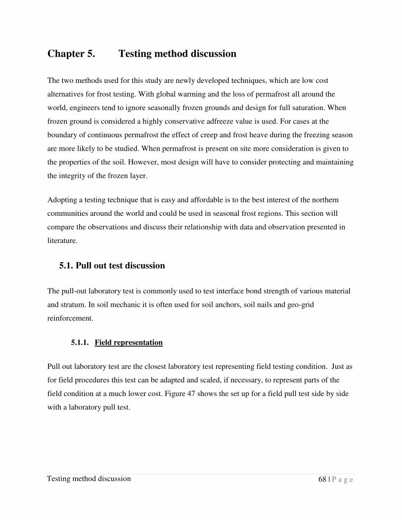
68 | P a g e
Testing method discussion
Chapter 5. Testing method discussion
The two methods used for this study are newly developed techniques, which are low cost
alternatives for frost testing. With global warming and the loss of permafrost all around the
world, engineers tend to ignore seasonally frozen grounds and design for full saturation. When
frozen ground is considered a highly conservative adfreeze value is used. For cases at the
boundary of continuous permafrost the effect of creep and frost heave during the freezing season
are more likely to be studied. When permafrost is present on site more consideration is given to
the properties of the soil. However, most design will have to consider protecting and maintaining
the integrity of the frozen layer.
Adopting a testing technique that is easy and affordable is to the best interest of the northern
communities around the world and could be used in seasonal frost regions. This section will
compare the observations and discuss their relationship with data and observation presented in
literature.
5.1. Pull out test discussion
The pull-out laboratory test is commonly used to test interface bond strength of various material
and stratum. In soil mechanic it is often used for soil anchors, soil nails and geo-grid
reinforcement.
5.1.1. Field representation
Pull out laboratory test are the closest laboratory test representing field testing condition. Just as
for field procedures this test can be adapted and scaled, if necessary, to represent parts of the
field condition at a much lower cost. Figure 47 shows the set up for a field pull test side by side
with a laboratory pull test.
69 | P a g e
Testing method discussion
Figure 47: Field pull test set up (left) lab pull out test (right)
Small scale testing is possible with the laboratory setup and multi-layered soils can also be
tested if necessary. The method is also versatile in its way to prepare and use different types of
piles and soil.
5.1.2. Test versatility
In addition to scaling and field representation, the pull-out test also proves easy to modify when
needed. The easiest and simplest parameters to modify for testing were water content and
embedded depth. The water content could range from completely dry to over-saturated or
submerged conditions, since the test box is fully enclosed and impermeable.
This method also allows for the user to quickly change the setup to test different types of pile
shape and materials. The only modification required is the type of attachments. Clamps can be
used with H-pile sections, an embedded bar can be installed in a concrete pile or a screw in bolt
can be installed on top of a lumber pile. The options are only dependent on the size and type of
the universal test machine available.
Since the testing box is a small-scale element of ground the installation process can also be
modified. For this study the piles were assumed to be augered and put-in-place. It is also possible
to install driven in place or mud back filled fill if necessary. This option is practical for concrete

70 | P a g e
Testing method discussion
and H-pile testing. It is known that the installation method has an important influence on the
bearing capacity of piles (Randolph et al., 1979; Johnston & Ladanyi, 1972) and most small
element laboratory test do not capture the effect of the installation process.
5.1.3. Test results
The behaviour for this type of adfreeze test procedure is comparable to field tests. They are
however complicated to compare to other results obtained by direct shearing. The data obtained
from this test is limited to displacement, depth and force. It is not an element model in which all
forces are known in all direction.
The test is easily scalable by modifying the physical properties like depth, size of pile and soil
layer. There are very limited ways to observe and collect data on the effect of lateral stress on the
pile (normal loads) or isolate local effects and conditions.
The data obtained is to be computed with depth as a main parameter. Weaver and Morgenstern
(1981) described those lateral normal forces on piles (effective stress) to be negligible with little
effect on the adfreeze bond. This statement was proven wrong by Ladanyi and Theriault in 1990
when they presented the effect of effective stress for different type of soil under freezing
conditions. This is an issue of importance when modelling the problem. While using finite
member element to model the pile under axial load could be done using those results, it is a lot
more complicated to modify the data to fit a finite element model.
5.1.4. Testing equipment
When it comes to laboratory testing, using large laboratory specimens like the ones needed for
this set up, is expensive and requires a lot of resources. The size of the test box alone is
considerable and requires planning for transportation, installation and storage. Laboratories don’t
typically have the storage or resources to equip themselves with large pieces of equipment that
are rarely used.
5.2. Soil Interface testing discussion
71 | P a g e
Testing method discussion
The interface shear testing is a method easily modified from standard simple shear test apparatus,
which are common in laboratories and easy to use.
5.2.1. Field representation
Simple shear tests are extensively used in soil mechanics. This type of test has been largely
studied. It has been found to show discrepancies with in-situ stress conditions (Prevost, 1976). It
does so due to the lateral stress induced by the walls of the shear box while under normal stress.
Prevost showed that the increase in normal stress is proportionate to the increase of those lateral
forces. In sand the effect is increased when shear distortion is imposed to the sample. This test
procedure is also known to induce additional stress by slippage.
Pure shear elements are rarely found under practical conditions. Simple shear and direct shear
test both shows the same issues but are commonly used to find design criteria even if they are not
accurate element representations of field conditions. An adaptation for interface testing under
triaxial condition is the optimal element representation. This type of test would be highly
expensive and complicated to develop.
The way samples are prepared and frozen under a constant normal stress is not highly
representative of the conditions found on site. No considerations are given to the stress and other
effects occurring during the pile installation process. In addition, there is no way to study the
effect of different shapes or cast in place piles.
5.2.2. Test versatility
Simple shear tests offer a very limited range of test conditions. The variable parameters of this
test are the application of normal stress and shear rate. It was found that due to the undrained
characteristics of this type of test, water content cannot be easily modified. The increase in pore
water pressure under high normal stress influences the freezing process and the increase in
internal stress due to the expansion of water between the particles.
72 | P a g e
Testing method discussion
The nature of frozen soils, where ice impedes free movement of water, does not allow for
drained and consolidated tests. In addition, there is no instrument in the apparatus for monitoring
pore water pressure buildup.
The stresses created by the installation and freezing process are known to dissipate over time. A
small sample would dissipate those stresses faster and represent long term strength. This effect
varies in the type of soil.
5.2.3. Test results
The data obtained from simple shear test can be manipulated and plotted in different ways.
Generating a Mohr circle and plotting the stress path is easy to do after a series of individual
tests. It is important to note the test is completed under undrained conditions. Even frozen, the
soil contains a liquid phase that is still able to influence local stress under undrained conditions.
5.2.4. Testing equipment
The testing equipment used for this study has been modified from a well-known testing process.
Any laboratory’s simple or direct shear apparatus can be used to test adfreeze bond with many
type of interfaces. Different steel plates, precast concrete or planks can be inserted in the
apparatus to act as pile material.
6.3 Data discussion
The data obtained by both techniques are not comparable. Not only regarding absolute values but
also on shape and response. The common published data available presents maximum and
residual values with only a description of the behaviour. Parameswaran (1978 & 1981) and
Ladanyi & Theriault (1990) have presented values using similar testing methods. Both using
saturated sands, the difference in the values publish shows similar variations. The push through
values ranged around 725 kPa for the same push rate against steel (Parameswaran 1981) while
the interface test yielded maximum adfreeze bonds in ranges of 140 kPa to 550 kPa (Ladanyi
1990) at high normal stresses.
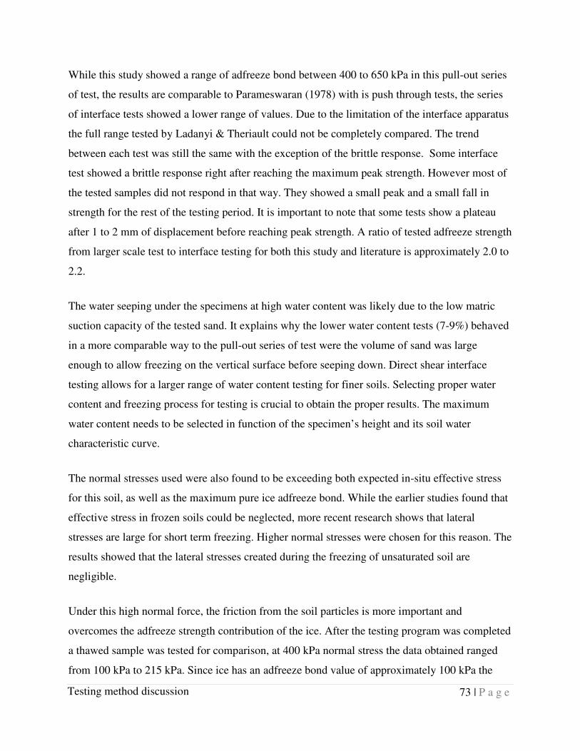
73 | P a g e
Testing method discussion
While this study showed a range of adfreeze bond between 400 to 650 kPa in this pull-out series
of test, the results are comparable to Parameswaran (1978) with is push through tests, the series
of interface tests showed a lower range of values. Due to the limitation of the interface apparatus
the full range tested by Ladanyi & Theriault could not be completely compared. The trend
between each test was still the same with the exception of the brittle response. Some interface
test showed a brittle response right after reaching the maximum peak strength. However most of
the tested samples did not respond in that way. They showed a small peak and a small fall in
strength for the rest of the testing period. It is important to note that some tests show a plateau
after 1 to 2 mm of displacement before reaching peak strength. A ratio of tested adfreeze strength
from larger scale test to interface testing for both this study and literature is approximately 2.0 to
2.2.
The water seeping under the specimens at high water content was likely due to the low matric
suction capacity of the tested sand. It explains why the lower water content tests (7-9%) behaved
in a more comparable way to the pull-out series of test were the volume of sand was large
enough to allow freezing on the vertical surface before seeping down. Direct shear interface
testing allows for a larger range of water content testing for finer soils. Selecting proper water
content and freezing process for testing is crucial to obtain the proper results. The maximum
water content needs to be selected in function of the specimen’s height and its soil water
characteristic curve.
The normal stresses used were also found to be exceeding both expected in-situ effective stress
for this soil, as well as the maximum pure ice adfreeze bond. While the earlier studies found that
effective stress in frozen soils could be neglected, more recent research shows that lateral
stresses are large for short term freezing. Higher normal stresses were chosen for this reason. The
results showed that the lateral stresses created during the freezing of unsaturated soil are
negligible.
Under this high normal force, the friction from the soil particles is more important and
overcomes the adfreeze strength contribution of the ice. After the testing program was completed
a thawed sample was tested for comparison, at 400 kPa normal stress the data obtained ranged
from 100 kPa to 215 kPa. Since ice has an adfreeze bond value of approximately 100 kPa the
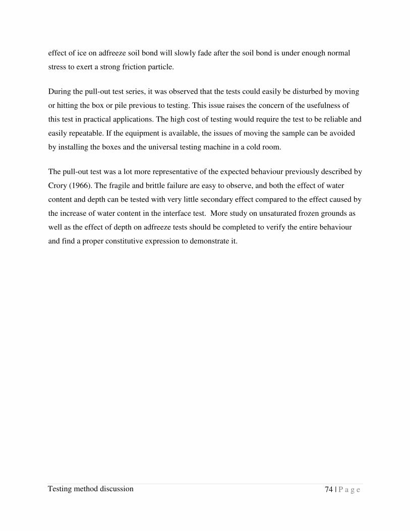
74 | P a g e
Testing method discussion
effect of ice on adfreeze soil bond will slowly fade after the soil bond is under enough normal
stress to exert a strong friction particle.
During the pull-out test series, it was observed that the tests could easily be disturbed by moving
or hitting the box or pile previous to testing. This issue raises the concern of the usefulness of
this test in practical applications. The high cost of testing would require the test to be reliable and
easily repeatable. If the equipment is available, the issues of moving the sample can be avoided
by installing the boxes and the universal testing machine in a cold room.
The pull-out test was a lot more representative of the expected behaviour previously described by
Crory (1966). The fragile and brittle failure are easy to observe, and both the effect of water
content and depth can be tested with very little secondary effect compared to the effect caused by
the increase of water content in the interface test. More study on unsaturated frozen grounds as
well as the effect of depth on adfreeze tests should be completed to verify the entire behaviour
and find a proper constitutive expression to demonstrate it.

75 | P a g e
Conclusion
Chapter 6. Conclusion
In conclusion, this study observed the various effects of unsaturated freezing including, water
migration, separation and fragile bonding.
1) The modifications made to Fakharian and Evgin (1996) interface apparatus allowed to
prepare, freeze and test specimen on place avoiding handling disturbances.
2) It was observed that unsaturated adfreeze strength shows the same behavior as previously
studied for saturated freezing.
3) After comparing literature data of similar testing procedures used for this study as well as
the data presented, it can be concluded that the results between large scale pull/push out
testing are not completely compatible.
4) The results obtained by direct interface shear testing proved both in literature and this
series of test to be smaller than the strength obtained from large scale testing. The results
of both types of tests are difficult to correlate, due in part to the unknown lateral normal
stresses existing on the embedded pile, A ratio of maximum adfreeze strength of 2.0 to
2.2 was observed.
5) The behavior of unsaturated frozen ground, bearing capacity and strength is closely
related to the water content. Once the saturation point is passed, the strength
characteristics tend towards pure ice properties.
6) Unsaturated frozen soils are submitted to lower effective stress due to their shallow depth
and the amount of void available for the water to expand while freezing.
The series of tests conducted under this study also observed a marked difference in the several
testing techniques used and the data available. This was to conclude if any techniques available
was economically viable. While larger scale test gives comparable results to field testing, they
require more resources. Interface shear testing uses more available testing apparatus and smaller
installation. Since frozen ground applications are rarely encountered interface testing would
provide the required data. Larger scale testing would be more suited for larger and more
complicated projects.

76 | P a g e
Conclusion
7.1 Suggestion for further studies
The interface apparatus developed by Fakharian and Evgin (1996) used for this study is a basic
version of the apparatus used by & Theriault (1990) for this application. A modern version of
these apparatuses should be developed. This updated version of the machine would not only be
useful for frozen soil applications but versatile enough for all interface shear testing.
1) Complete a series of saturated and over-saturated test using the large-scale pull-out
method to compare the hypotheses suggested.
2) Complete a series of test freezing the interface under a gradient of temperature to
simulate the effect of freeze piles and thermosyphon.
3) Observe the effect of freeze thaw cycles on adfreeze bond and the effect each cycle has
on the strength of the bond.
4) Complete a similar series of test using a fine grain soil to observe the effect matric
suction has on the freezing process
5) Observe the field requirement and testing procedure do better approach the practical side
of the design

77 | P a g e
References
References
− Aldaeef A.A., Rayhani M.T. (2018) Adfreeze Strength and Creep Behavior of Pile
Foundations in Warming Permafrost. In: Abu-Farsakh M., Alshibli K., Puppala A. (eds)
Advances in Analysis and Design of Deep Foundations. GeoMEast 2017. Sustainable
Civil Infrastructures. Springer, Cham
− Andersland, O. B., & Ladanyi, B. (2004). Frozen ground engineering. John Wiley &
Sons.
− Arenson, L. U., Springman, S. M., & Sego, D. C. (2007). The rheology of frozen soils.
Applied Rheology, 17(1), 12147.
− Arenson, L.U. and Springman, S.M.(2005) Mathematical description for the behaviour
of ice-rich frozen soils at temperatures close to zero centigrade. Canadian Geotechnical
Journal 42 431-442.
− Arteau, J. (1984) Étude de la consolidation des sols gelés. Ph.D. diss., École
Polytechnique, Montreal.
− Baker, T.H.W. (1976). Transportation, preparation and storage of frozen soil samples for
laboratory testing. In Soil Specimen Preparation for Laboratory Testing. ASTM Spec.
Tech. Pub. 559, pp.88-112
− Bishop, A.W. (1973) The influence of an undrained change in stress on pore pressure in
porous media of low compressibility. Géotechnique 23(3):435-42
− Black, P. B., & Tice, A. R. (1989). Comparison of soil freezing curve and soil water
curve data for Windsor sandy loam. Water Resources Research, 25(10), 2205-2210.
− Catana, M. C. (2006). Compaction and water retention characteristics of Champlain sea
clay (Doctoral dissertation, University of Ottawa (Canada)).
− Crory, F. E. (1966). Pile foundations in permafrost. In Permafrost: Proceedings of North
American Contribution to First International Conference on Permafrost (pp. 467-476).
− Domaschuk, L. (1982). Frost heave forces on embedded structural units. In Proceedings
of 4th Canadian Permafrost Conference (pp. 487-496).

78 | P a g e
References
− Faizi, K., Kalatehjari, R., Nazir, R., & Rashid, A. S. A. (2015). Determination of pile
failure mechanism under pullout test in loose sand. Journal of Central South University,
22(4), 1490-1501.
− Fakharian, K., and E. Evgin. "A three-dimensional apparatus for cyclic testing of
interfaces." Proc. 46th Annual Canadian Geotechnical Conference. 1993.
− Fakharian, K. and Evgin, E., "An Automated Apparatus for Three-Dimensional
Monotonic and Cyclic Testing of Interfaces," Geotechnical Testing Journal, Vol. 19, No.
1, 1996, pp. 22-31, https://doi.org/10.1520/GTJ11404J. ISSN 0149-6115
− Gold, L.W., (1970) Process of failure in ice. Canadian Geotechnical Journal 7 405-413.
− Goodman,M.A. (1975). Mechanical properties of simulated deep permafrost. ASME J.
Eng. Ind. Ser. B 97(2):417-25
− Hammer, T. A., Ryan, W. L., & Zirjacks, W. L. (1985). Ground temperature
observations. In Thermal Analysis,Construction, and Monitoring Methods for Frozen
Ground (pp. 9-46). ASCE.
− Harris, S.A. (2015). Permafrost. In the Canadian Encyclopedia. Retrieved from
http://www.thecanadianencyclopedia.ca
− Heydinger, A. G. (1987). Piles in permafrost. Journal of cold regions engineering, 1(2),
59-75.
− Hillel, D. (1980) Applications of Soil Physics. New York: Academic Press.
− Johnston, G. H., & Ladanyi, B. (1972). Field tests of grouted rod anchors in permafrost.
Canadian Geotechnical Journal, 9(2), 176-194.
− Kelly, R. B., Houlsby, G. T., & Byrne, B. W. (2006). A comparison of field and
laboratory tests of caisson foundations in sand and clay.
− Koopmans, R. W. R., & Miller, R. D. (1966). Soil freezing and soil water characteristic
curves. Soil Science Society of America Journal, 30(6), 680-685.
− Ladanyi, B. (1985) Stress transfer mechanism in frozen soils. Invited lecture. In 10th
Canadian Congress on Applied Mechanics, London, Ontario, Canada, vol. 1, pp. 11-15.
− Ladanyi. B. (2002). Behavior of ice-rock mixture on slopes. 11th Int. Conf on cold
regions Engrg., Anchorage, Alaska:632-699.

79 | P a g e
References
− Ladanyi, B. (2003). Rheology of ice/rock systems and interfaces. In Proceedings of the
8th International Conference on Permafrost, Zurich (pp. 22-25).
− Ladanyi,B., and G.H. Johnston. (1978) Field investigations of frozen ground. Chap. 9 in
Geotechnical Engineering for Cold Regions, ed. O.B Anderlsand and D.M. Anderson.
New York: McGraw-Hill
− Ladanyi, B., & Theriault, A. (1990). A study of some factors affecting the adfreeze bond
of piles in permafrost. In Proc. of Geotechnical Engineering Congress GSP (Vol. 27, pp.
213-224).
− Marcuson III, W. F., & Franklin, A. G. (1979). State of the art of undisturbed sampling of
cohesionless soils (No. WES-MP-GL-79-16). Army Engineer Waterways Experiment
Station Vicksburg MS.
− Miller, R. D. (1965). Phase equilibria and soil freezing. In Permafrost: Proceedings of the
Second International Conference. Washington DC: National Academy of Science-
National Research Council (Vol. 287, pp. 193-197).
− Miller, D. L. (1985). Temperature Monitoring/Ground Thermometry. In Thermal
Analysis,Construction, and Monitoring Methods for Frozen Ground(pp. 57-75). ASCE.
− Nixon, J. F., & McRoberts, E. C. (1976). A design approach for pile foundations in
permafrost. Canadian Geotechnical Journal, 13(1), 40-57.
− Nottingham, D. & Christopherson, A.B. (1983) Design Criteria for Driven Piles in
Permafrost. Department of Transport and Public Facilities
− Palmeria, E. M., & Milligan, G. W. E. (1989). Scale and other factors affecting the results
of pull-out tests of grids buried in sand. Geotechnique, 39(3), 511-542.
− Parameswaran, V. R. (1978). Adfreeze strength of frozen sand to model piles. Canadian
geotechnical journal, 15(4), 494-500.
− Parameswaran, V. R. (1981). Adfreeze strength of model piles in ice. Canadian
Geotechnical Journal, 18(1), 8-16.
− Phuong, N. T. V., Van Tol, A. F., Elkadi, A. S. K., & Rohe, A. (2016). Numerical
investigation of pile installation effects in sand using material point method. Computers
and Geotechnics, 73, 58-71.

80 | P a g e
References
− Phukan, A.(1978) Pile Foundations in Frozen Soils. Journal of Pressure Vessel
Technology 100, no. 3 : 302–9. doi:10.1115/1.3454471.
− Prevost, J. H., & Høeg, K. (1976). Reanalysis of simple shear soil testing. Canadian
Geotechnical Journal, 13(4), 418-429.
− Randolph, M. F., Carter, J. P., & Wroth, C. P. (1979). Driven piles in clay—the effects of
installation and subsequent consolidation. Geotechnique, 29(4), 361-393.
− Rostami, H. (2017). Finite Element Analysis of Coupled Thermo-Hydro-Mechanical
Processes in Fully Saturated, Partially Frozen Soils (Master's thesis, NTNU).
− Saeki, H. (2011). Mechanical Properties Between Ice and Various Materials Used in
Hydraulic Structures: The Jin S. Chung Award Lecture, 2010. International Journal of
Offshore and Polar Engineering, 21(02).
− Sheikhtaheri, M. (2014). Experimental and numerical modeling studies for interpreting
and estimating the p–δ behavior of single model piles in unsaturated sands (Doctoral
dissertation, Université d'Ottawa/University of Ottawa).
− Spaans, E. J., & Baker, J. M. (1996). The soil freezing characteristic: Its measurement
and similarity to the soil moisture characteristic. Soil Science Society of America Journal,
60(1), 13-19.
− Stähli, M. (2005). Freezing and thawing phenomena in soils. Encyclopedia of
hydrological sciences.
− Ting, J.M., Martin, R.T. &Ladd, C.C. (1983). Mechanisms of strength for frozen sand. J.
Geotech. Engrg., ASCE 109(10):1286-1302.
− Veillette, J. (1975). Helicopter portable drill for high artic programs. Geol. Surv. Can.
Pap. 75-1, pt .A.
− Weaver, J. S., & Morgenstern, N. R. (1981). Pile design in permafrost. Canadian
Geotechnical Journal, 18(3), 357-370.
− Wissa, A.E.Z. (1969) Pore pressure measurement in saturated stiff soils. J.Soil Mech.
Found. Civ. ASCE95(SM4): 1063-73
− Xu, X. T., Liu, H. L., & Lehane, B. M. (2006). Pipe pile installation effects in soft clay.
Proceedings of the Institution of Civil Engineers-Geotechnical Engineering, 159(4), 285-
296.

81 | P a g e
References
− Yong, R. N. (1962). Research on Fundamental Properties of Frozen Soils. Proc. 1st
Canadian Conf. Permafrost, pp. 84-108.
− Zhang, T., Barry, R. G., Knowles, K., Ling, F., & Armstrong, R. L. (2003, July).
Distribution of seasonally and perennially frozen ground in the Northern Hemisphere. In
Proceedings of the 8th International Conference on Permafrost (Vol. 2, pp. 1289-1294).
AA Balkema Publishers.

82 | P a g e
Pull out test results
Appendix A. Pull out test results
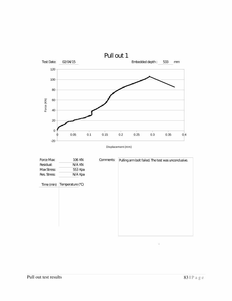
83 | P a g e
Pull out test results
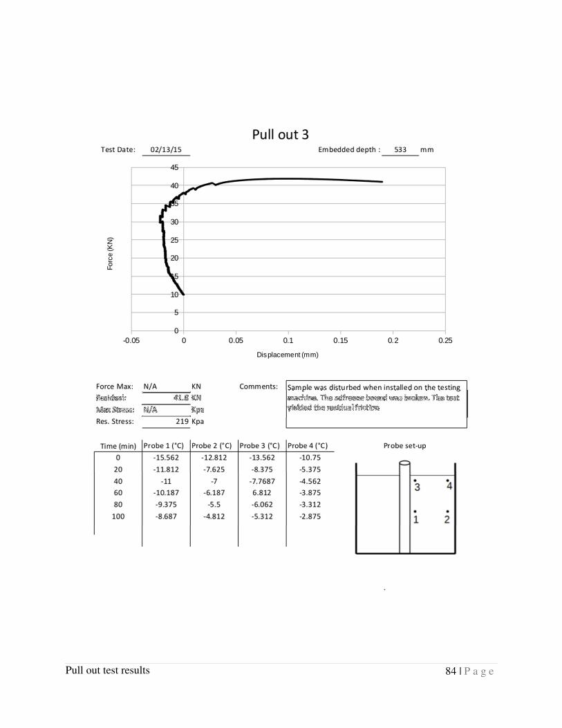
84 | P a g e
Pull out test results

85 | P a g e
Pull out test results
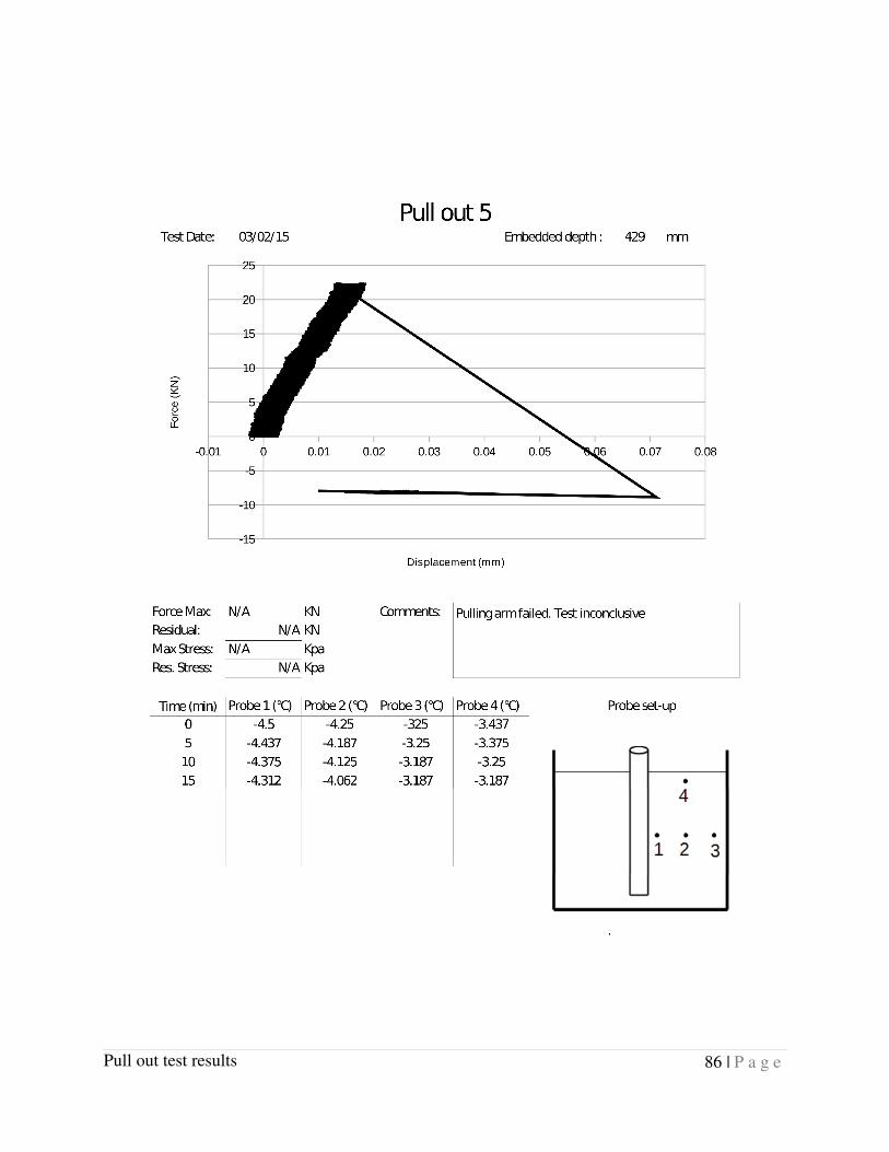
86 | P a g e
Pull out test results

87 | P a g e
Pull out test results
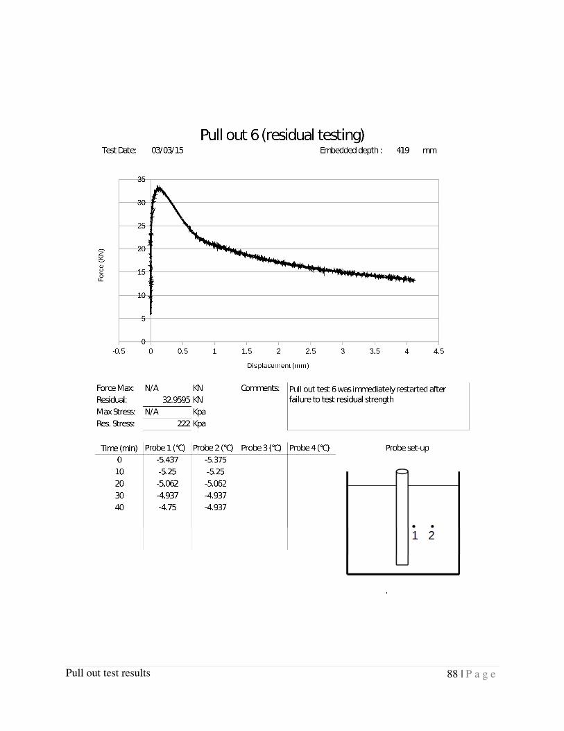
88 | P a g e
Pull out test results

89 | P a g e
Pull out test results

90 | P a g e
Pull out test results

91 | P a g e
Pull out test results
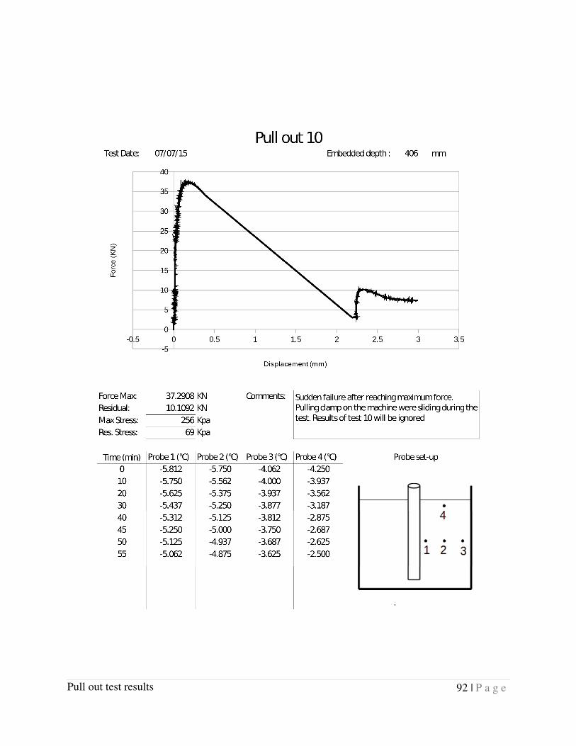
92 | P a g e
Pull out test results
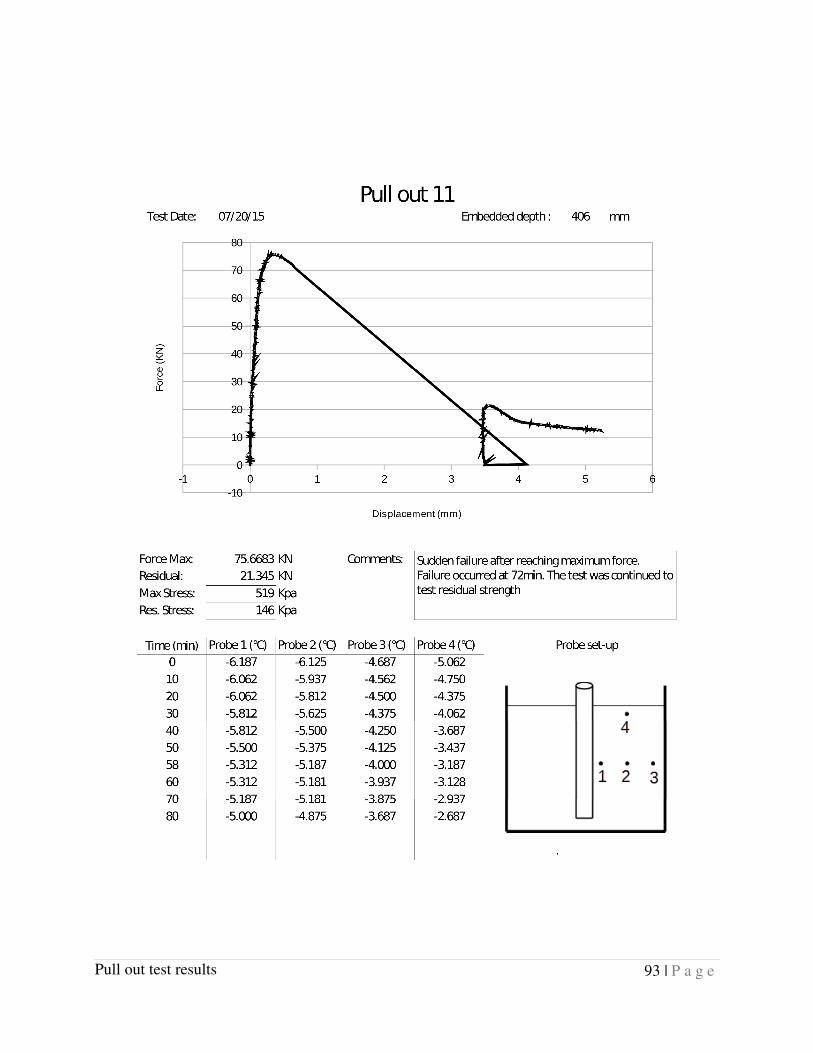
93 | P a g e
Pull out test results

94 | P a g e
Pull out test results
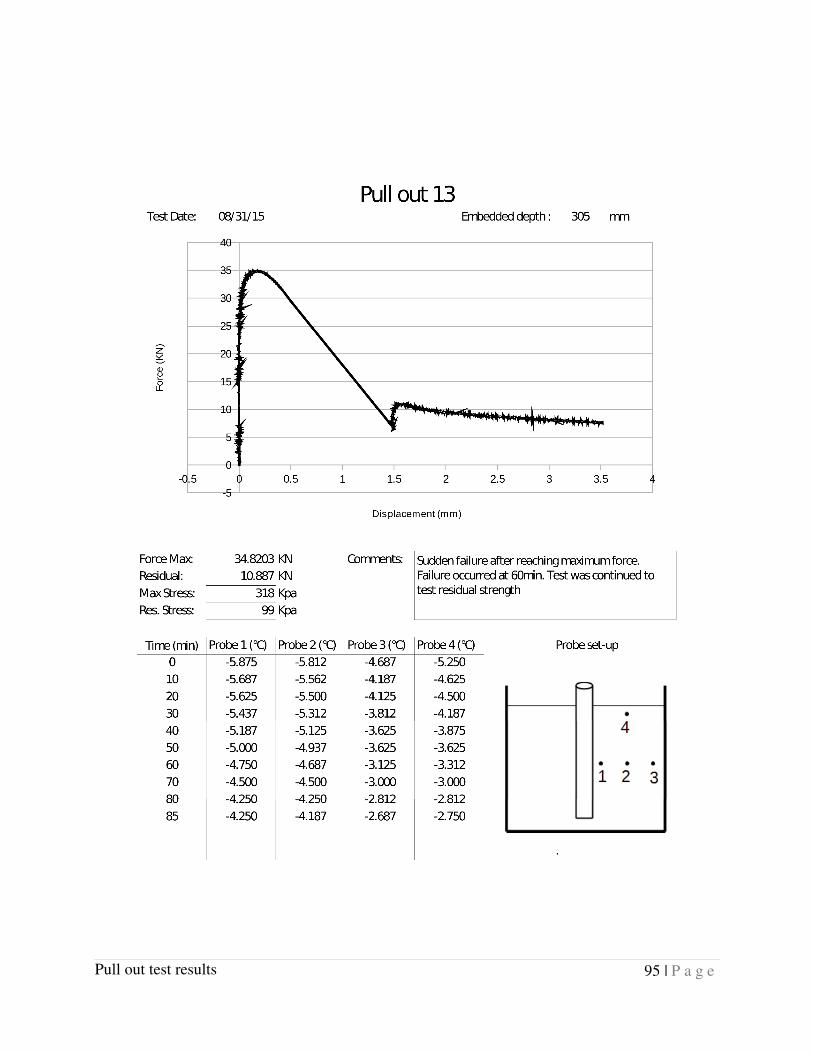
95 | P a g e
Pull out test results

96 | P a g e
Pull out test results

97 | P a g e
Interface test results
Appendix B. Interface test results
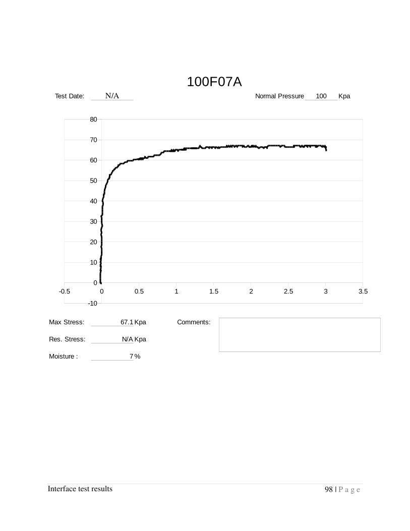
98 | P a g e
Interface test results
100F07ATest Date: N/A Normal Pressure 100 Kpa
Max Stress: 67.1 Kpa Comments:
Res. Stress: N/A Kpa
Moisture : 7 %
-0.5 0 0.5 1 1.5 2 2.5 3 3.5
-10
0
10
20
30
40
50
60
70
80

99 | P a g e
Interface test results
150F07ATest Date: N/A Normal Pressure 150 Kpa
Max Stress: 103.0 Kpa Comments:
Res. Stress: N/A Kpa
Moisture : 7 %
-0.5 0 0.5 1 1.5 2 2.5
-20
0
20
40
60
80
100
120

100 | P a g e
Interface test results
300F07ATest Date: N/A Normal Pressure 300 Kpa
Max Stress: 183.0 Kpa Comments:
Res. Stress: N/A Kpa
Moisture : 7 %
-0.5 0 0.5 1 1.5 2 2.5 3 3.5
-50
0
50
100
150
200
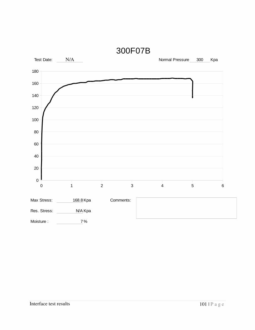
101 | P a g e
Interface test results
300F07BTest Date: N/A Normal Pressure 300 Kpa
Max Stress: 168.8 Kpa Comments:
Res. Stress: N/A Kpa
Moisture : 7 %
0 1 2 3 4 5 6
0
20
40
60
80
100
120
140
160
180
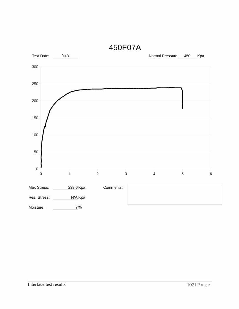
102 | P a g e
Interface test results
450F07ATest Date: N/A Normal Pressure 450 Kpa
Max Stress: 238.6 Kpa Comments:
Res. Stress: N/A Kpa
Moisture : 7 %
0 1 2 3 4 5 6
0
50
100
150
200
250
300

103 | P a g e
Interface test results
350F09ATest Date: 14/04/16 Normal Pressure 350 Kpa
Max Stress: 176 Kpa Comments:
Res. Stress: N/A Kpa
Moisture : 9 %
0 1 2 3 4 5 6
0
20
40
60
80
100
120
140
160
180
200
Displacement (mm)
Str
ess (
KP
a)
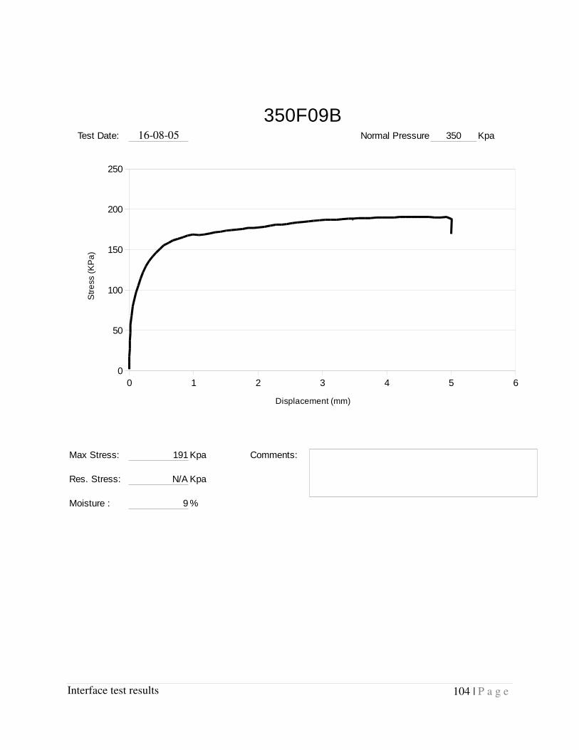
104 | P a g e
Interface test results
350F09BTest Date: 16-08-05 Normal Pressure 350 Kpa
Max Stress: 191 Kpa Comments:
Res. Stress: N/A Kpa
Moisture : 9 %
0 1 2 3 4 5 6
0
50
100
150
200
250
Displacement (mm)
Str
ess (
KP
a)

105 | P a g e
Interface test results
350F09ITest Date: 16-09-07 Normal Pressure 350 Kpa
Max Stress: 296 Kpa Comments:
Res. Stress: 111.2 Kpa
Moisture : 9 %
-1 0 1 2 3 4 5 6 7
-50
0
50
100
150
200
250
300
350
Displacement (mm)
Str
ess (
KP
a)

106 | P a g e
Interface test results
400F09ATest Date: 13/04/16 Normal Pressure 400 Kpa
Max Stress: 247 Kpa Comments:
Res. Stress: N/A Kpa
Moisture : 9 %
0 1 2 3 4 5 6
0
50
100
150
200
250
300
Displacement (mm)
Str
ess (
KP
a)

107 | P a g e
Interface test results
450F09ATest Date: 13/04/16 Normal Pressure 450 Kpa
Max Stress: 286.1 Kpa Comments:
Res. Stress: N/A Kpa
Moisture : 9 %
0 1 2 3 4 5 6 7
0
50
100
150
200
250
300
350
Displacement (mm)
Str
ess (
KP
a)

108 | P a g e
Interface test results
400F11ATest Date: 20/06/016 Normal Pressure 400 Kpa
Max Stress: 177.6 Kpa Comments: Error with LVDT reading.
Res. Stress: N/A Kpa
Moisture : 11 %
0 50 100 150 200 250 300 350
0
20
40
60
80
100
120
140
160
180
200
Time (s)
Str
ess (
KP
a)

109 | P a g e
Interface test results
400F11ITest Date: 24/06/16 Normal Pressure 400 Kpa
Max Stress: 52.9 Kpa Comments:
Res. Stress: 29.8 Kpa
Moisture : 11 %
Table hit the stopper at the end of the linear bearing. Readjusted position for nex t test
0 1 2 3 4 5 6 7
0
10
20
30
40
50
60
70
80
Displacement (mm)
Str
ess (
KP
a)

110 | P a g e
Interface test results
400F11JTest Date: 25/06/16 Normal Pressure 400 Kpa
Max Stress: 195.2 Kpa Comments:
Res. Stress: 105.1 Kpa
Moisture : 11 %
0 1 2 3 4 5 6 7
0
50
100
150
200
250
Displacement (mm)
Str
ess (
KP
a)

111 | P a g e
Interface test results
400F11KTest Date: 26/06/16 Normal Pressure 400 Kpa
Max Stress: 185.1 Kpa Comments:
Res. Stress: N/A Kpa
Moisture : 11 %
-1 0 1 2 3 4 5 6 7
0
20
40
60
80
100
120
140
160
180
200
Displacement (mm)
Str
ess (
KP
a)

112 | P a g e
Interface test results
450F11ATest Date: 25/05/16 Normal Pressure 450 Kpa
Max Stress: 237.3 Kpa Comments:
Res. Stress: N/A Kpa
Moisture : 11 %
0 1 2 3 4 5 6
0
50
100
150
200
250
Displacement (mm)
Str
ess (
KP
a)

113 | P a g e
Interface test results
450F11ITest Date: 25/08/16 Normal Pressure 450 Kpa
Max Stress: 294.9 Kpa Comments:
Res. Stress: 219.7 Kpa
Moisture : 11 %
0 1 2 3 4 5 6 7
0
50
100
150
200
250
300
350
Displacement (mm)
Str
ess (
KP
a)

114 | P a g e
Interface test results
450F11MTest Date: 28/08/16 Normal Pressure 450 Kpa
Max Stress: 229.8 Kpa Comments:
Res. Stress: 127.5 Kpa
Moisture : 11 %
-0.5 0 0.5 1 1.5 2 2.5 3 3.5 4
-50
0
50
100
150
200
250
Displacement (mm)
Str
ess (
KP
a)

115 | P a g e
Interface test results
350F11ITest Date: 16-11-08 Normal Pressure 450 Kpa
Max Stress: 450.8 Kpa Comments:
Res. Stress: 120.0 Kpa
Moisture : 11 %
0 1 2 3 4 5 6
-100
0
100
200
300
400
500
Displacement (mm)
Str
ess (
KP
a)

116 | P a g e
Interface test results
350F13ITest Date: 16-11-08 Normal Pressure 350 Kpa
Max Stress: 143 Kpa Comments:
Res. Stress: N/A Kpa
Moisture : 13 %
0 0.5 1 1.5 2 2.5 3 3.5 4 4.5 5
0
20
40
60
80
100
120
140
160

117 | P a g e
Interface test results
450F13ATest Date: 16-11-08 Normal Pressure 450 Kpa
Max Stress: 155 Kpa Comments:
Res. Stress: N/A Kpa
Moisture : 13 %
0 1 2 3 4 5 6
0
20
40
60
80
100
120
140
160
180

118 | P a g e
Pull out Setup Drawings
Appendix C. Pull out Setup Drawings

119 | P a g e
Pull out Setup Drawings

120 | P a g e
Pull out Setup Drawings

121 | P a g e
Pull out Setup Drawings