Laboratory for Media Processing - National Chiao Tung …people.cs.nctu.edu.tw/~cmliu/Courses/audio/chap1-2.pdfNCTU/CSIE/DSP LAB Audio Processing Group Definition Backgrounds3 Signals

NCTU/CSIE/DSP LABAudio Processing Group

Backgrounds11 IntroductionSignals, Systems, and Digital Signal Processing

DefinitionBasic Elements of a Digital Signal ProcessingAdvantages of Digital over Analog Signal Processing

Classification of SignalsMulti-channel and Multi-dimensional SignalsContinuous-Time versus Discrete-Time SignalsContinuous-Valued versus Discrete-Valued Signals

Concepts of FrequencyPhysical Interpretation of Signal Frequency Continuous-Time Sinusoidal SignalsDiscrete-Time Sinusoidal Signals


Backgrounds2

1.1 Signals, Systems, & Digital Signal ProcessingDefinitionBasic Elements of DSPAdvantages of Digital over Analog Signal Processing


Backgrounds3DefinitionSignals

Any physical quantity that varies with time, space or any other independent variable.Communication beween humans and machines.

Systemsmathematically a transformation or an operator that maps an input signal into an output signal.can be either hardware or software.such operations are usually referred as signal processing.

Digital Signal ProcessingThe representation of signals by sequences of numbers or symbols and the processing of these sequences.


Backgrounds4

Basic Elements of a Digital Signal Processing System A/D Converter

Converts an analog signal into a sequence of digits

D/A ConverterConverts a sequence of digits into an analog signal

AnalogInputSignal

A/D Converter

A/D Converter

DigitalInputSignal

D/A Converter

D/A Converter

DigitalSignal

Processing

DigitalSignal

Processing0

t 3, 5, 4, 6 ...

AnalogOutputSignal

DigitalOutputSignal


Backgrounds5Advantages of Digital over Analog ProcessingBetter control of accuracyEasily stored on magnetic mediaAllow for more sophisticated signal processingCheaper in some cases


Backgrounds61.2 Classification of SignalsMultichannel versus Multidimensional Signals

Signals may be generated by multiple sources or multiple sensors. Such signals are multi-channel signals.A signal which is a function of M independent variables is called multi-dimensional signals.

Continuous-Time versus Discrete-Time SignalsContinuous-time signals are defined for every value of time.Discrete -time signals are defined at discrete values of time.

Continuous-Valued versus Discrete-Valued SignalsA signal which takes on all possible values on a finite range or infinite range is said to be a multi-channel signal.A signal takes on values from a finite set of possible values is said to be a multi-dimensionall signal.


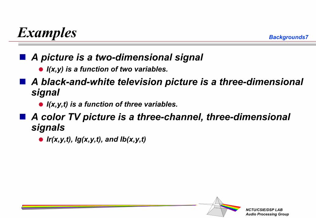
Backgrounds7ExamplesA picture is a two-dimensional signal

I(x,y) is a function of two variables.

A black-and-white television picture is a three-dimensional signal

I(x,y,t) is a function of three variables.

A color TV picture is a three-channel, three-dimensional signals

Ir(x,y,t), Ig(x,y,t), and Ib(x,y,t)


Backgrounds81.3 1.3 Concepts of FrequencyConcepts of Frequency

Physical Interpretation of Signal FrequencyContinuous-Time Sinusoidal SignalsDiscrete-Time Sinusoidal Signals


Backgrounds9

Physical Interpretation of Signal Physical Interpretation of Signal FrequencyFrequency

A familiar term in physics and mathematics A familiar term in physics and mathematics Radio transmitter/receiverRadio transmitter/receiverAmplifierAmplifierColor photographyColor photography

..............................


Backgrounds10Physical Interpretation of Signal FrequencyInterpretation

Closed related to a specific type of periodic motion called harmonic oscillation, described by sinusoidal functions.Usually a dimension of inverse time.

Time

Why is the term important ?


Backgrounds11

Physical Interpretation of Signal Physical Interpretation of Signal FrequencyFrequency

An ObservationAn ObservationTime DomainRepresentation

Frequency-DomainRepresentationFourier Transform


Backgrounds12Physical Interpretation of Signal Physical Interpretation of Signal

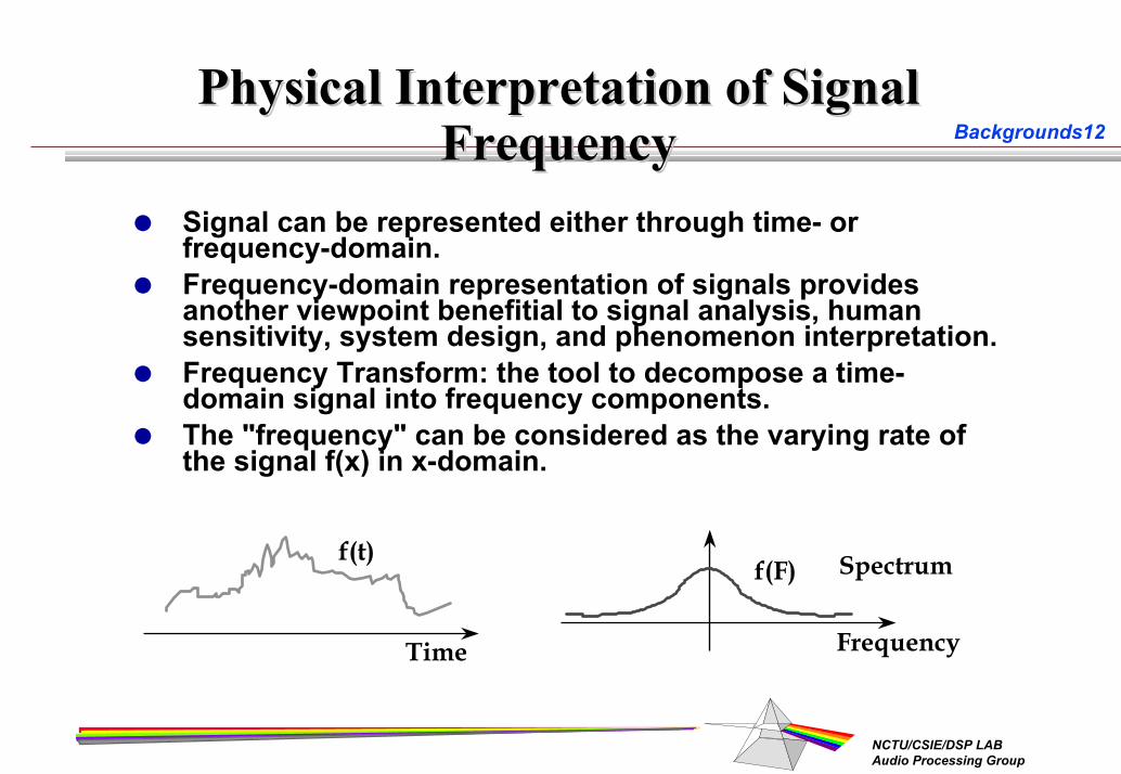
FrequencyFrequencySignal can be represented either through time- or frequency-domain.Frequency-domain representation of signals provides another viewpoint benefitial to signal analysis, human sensitivity, system design, and phenomenon interpretation.Frequency Transform: the tool to decompose a time-domain signal into frequency components.The "frequency" can be considered as the varying rate of the signal f(x) in x-domain.

f(t)

Time Frequency

f(F) Spectrum


Backgrounds131.3 Concepts of FrequencyPhysical Interpretation of Signal FrequencyContinuous-Time Sinusoidal SignalsDiscrete-Time Sinusoidal Signals


Backgrounds14

ContinuousContinuous--Time Sinusoidal SignalsTime Sinusoidal Signals

DefinitionXa(t) = A cos( Ω t+ θ)-*<t<*– A is the amplitude of the sinusoid– Ω is the frequency in radians per

second– θ is the phase in radians– F=Ω/2π is the frequency in

cycles per second or hertzTime

∞


Backgrounds15Continuous-Time Sinusoidal Signals (Cont.)For every fixed value of F, Xa(t) is periodic

Xa(t+Tp) = Xa(t), Tp=1/F

Continuous-time sinusoidal signals with distinct frequencies are themselves distinctIncreasing the frequency F results in an increase in the rate of oscillation


Backgrounds16DiscreteDiscrete--Time Sinusoidal SignalsTime Sinusoidal Signals

DefinitionX(n) = A cos( ω n+ θ), -*<t<*– A is the amplitude of the sinusoid– ω is the frequency in radians per second– θ is the phase in radians– f=ω/2π is the frequency in cycles per

second or hertz

X(n) = A cos( ω n+ θ)


Backgrounds17

DiscreteDiscrete--Time Sinusoidal Time Sinusoidal Signals(Cont.)Signals(Cont.)

A discrete-time sinusoidal is periodic only if its frequency f is a rational number– X(n+N) = X(n), N=p/f, where p is an

integerDiscrete-time sinusoidal signals where frequencies are separated by an integer multiple of 2π are identical– X1(n) = A cos( ω0 n)– X2(n) = A cos( (ω0 +2π) n)

The highest rate of oscillation in a discrete-time sinusoidal is attained when ω=π or (ω=-π), or equivalently f=1/2.– X(n) = A cos(( ω0+π)n) = -A cos((ω0+π)n

X(n) = A cos( ω n+ θ)


Backgrounds182. The Process of A/D and D/A ConversionThe Process of A/D and D/A ConversionBasic ElementsSignal SamplingAnti-aliasing FilteringQuantizationInterpolatorSmoothing Filters


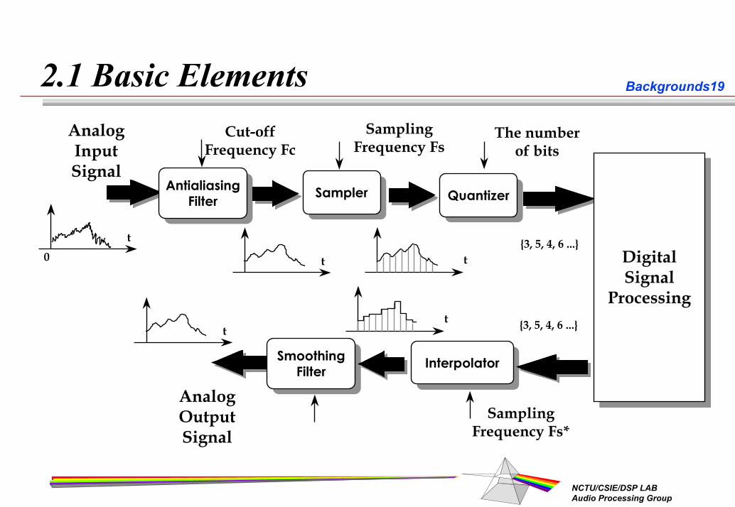
Backgrounds192.1 Basic ElementsSampling

Frequency Fs

0

t

AnalogInputSignal

Cut-off Frequency Fc

The number of bits

AntialiasingFilter

AntialiasingFilter SamplerSampler QuantizerQuantizer

SmoothingFilter

SmoothingFilter InterpolatorInterpolator

DigitalSignal

Processing

DigitalSignal

Processing

tt3, 5, 4, 6 ...

tt 3, 5, 4, 6 ...

AnalogOutputSignal

Cut-off Frequency Fc*

Sampling Frequency Fs*


Backgrounds202.1 Basic Elements(c.1)An Observation

The mapping between discrete-frequency and analog-frequency is one-to many


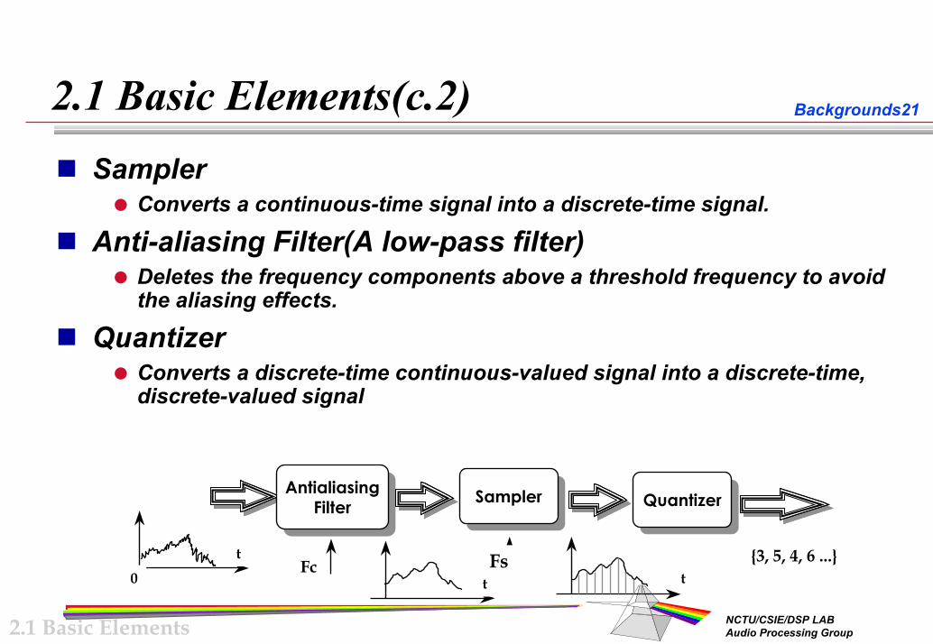
Backgrounds212.1 Basic Elements(c.2)Sampler

Converts a continuous-time signal into a discrete-time signal.

Anti-aliasing Filter(A low-pass filter)Deletes the frequency components above a threshold frequency to avoid the aliasing effects.

QuantizerConverts a discrete-time continuous-valued signal into a discrete-time, discrete-valued signal

2.1 Basic Elements

AntialiasingFilter


0

t

tt

3, 5, 4, 6 ...FsFc


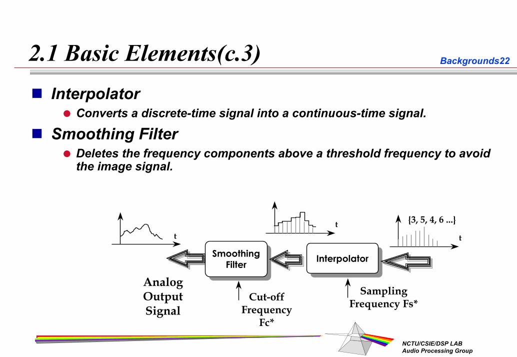
Backgrounds222.1 Basic Elements(c.3)Interpolator

Converts a discrete-time signal into a continuous-time signal.

Smoothing FilterDeletes the frequency components above a threshold frequency to avoid the image signal.


SmoothingFilter


AnalogOutputSignal

3, 5, 4, 6 ...

t

Cut-off Frequency

Fc*

tt


Backgrounds232.1 Basic Elements(c.4)Sampling

Frequency Fs

0

t

AnalogInputSignal


The number of bits

AntialiasingFilter

AntialiasingFilter SamplerSampler Quantizer

& CoderQuantizer& Coder

SmoothingFilter


DigitalSignal

Processing

DigitalSignal

Processing

tt3, 5, 4, 6 ...

tt 3, 5, 4, 6 ...

AnalogOutputSignal

Cut-off Frequency

Fc*



Backgrounds242.2 Signal Sampling

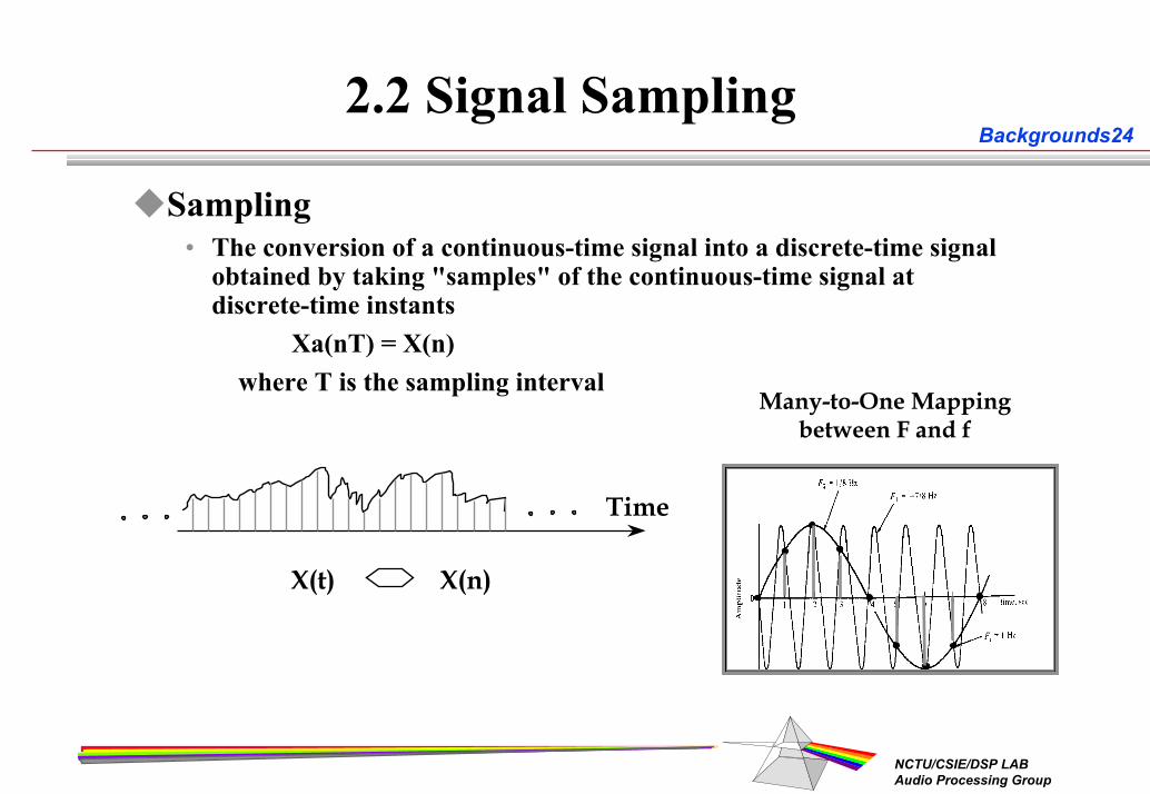
Sampling• The conversion of a continuous-time signal into a discrete-time signal

obtained by taking "samples" of the continuous-time signal at discrete-time instants

Xa(nT) = X(n)where T is the sampling interval

Many-to-One Mappingbetween F and f

Time

X(t) X(n)


Backgrounds25

2.2 Signal Sampling (c.1)Analog Frequency <==> Discrete Frequency

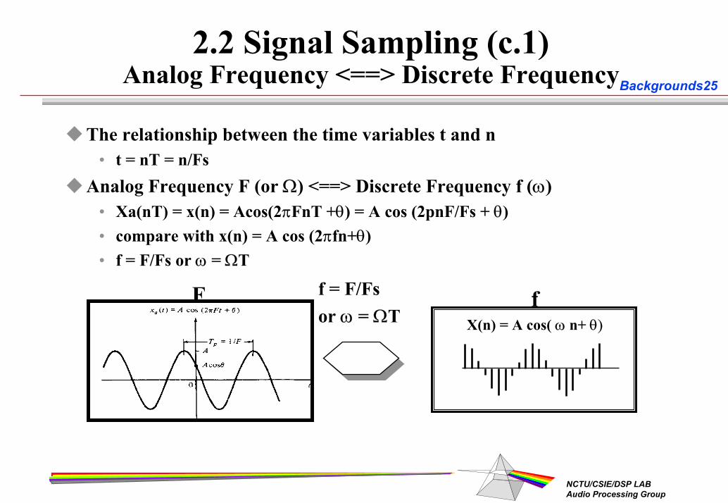
The relationship between the time variables t and n• t = nT = n/Fs

Analog Frequency F (or Ω) <==> Discrete Frequency f (ω)• Xa(nT) = x(n) = Acos(2πFnT +θ) = A cos (2pnF/Fs + θ)• compare with x(n) = A cos (2πfn+θ)• f = F/Fs or ω = ΩT

f = F/Fs or ω = ΩT

FX(n) = A cos( ω n+ θ)

f


Backgrounds26

2.2 Signal Sampling (c.2)Frequency Restriction

Continuous-Time Frequency- ∗ < F < - * < Ω <

Discrete-Time Frequency- 1/2 < f < 1/2- π < ω < π

Relation and Restriction- Fs/2 < F < Fs/2- πFs < Ω < πFs

Many-to-One Mapplingbetween F and f


Backgrounds27

2.2 Signal Sampling (c.3)Frequency Relation

Many-to-one MappingFk = F0 + kFs are indistinguishable from the frequency F0 afterresampling and hence they are aliased of F0.

Folding Frequency ==> Fs/2

0Fs/2 Fs-Fs -Fs/2

F

f


Backgrounds282.2 Signal Sampling (c.4)

Sampling Theorem• If the highest frequency contained in an analog signal Xa(t) is

Fmax =B and the signal is sampled at a rate Fs > 2Fmax = B, then Xa(t) can be exactly recovered from its sample values using the interpolation

g t BtBt

( ) sin=

22

ππ

Thus Xa(t) may be expressed as

a an s

x t X n Fs g t nF

( ) ( / ) ( )= −=−∞

∞

∑where Xa(n/Fs) = Xa(nT) = X(n) are the sample of Xa(t)



HistoryCauchy, French, 1841– Functions could be nonuniformly sampled and averaged over a long

period. Whittaker, Scottish, 1915– A bandlimited function can be completely reconstructed from

samples. (first mathematical proof of a general sampling theorem)K. Ogura, Japanese, 1920– If a function is sampled at a frequency at least twice the highest

function frequency, the samples contain all the information in the function, and can reconstruct the function.

Carson, American, 1920– Unpublished proof that related the same result to communication.



History (c.1)Nyquist, Sweden, 1928– For complete signal reconstruction, the required frequency bandwidth

is proportional to the signalling speed.– The minimum bandwidth is equal to half the number of code elements

per second.– Expressed the theorem in terms that are familiar to communication

engineers.Kotelnikov, Russian, 1933– A proof of sampling theorem

Shannon, American, 1949– Unified many aspects of sampling and founded the larger science of

information theory.


Backgrounds312.3 Antialiasing FiltersAliasing

F +- kFs are mapped into the same discrete frequency

0Fs/2 Fs-Fs -Fs/2

F

f


Backgrounds322.3 2.3 AntialiasingAntialiasing FiltersFilters

Purpose: Purpose: Delete the frequency components that will be aliased to low frequency components.

LowLow--Pass FiltersPass FiltersFcFc < Fs/2< Fs/2Fc

Low-Pass Filter

F

1


Backgrounds332.4 Quantization

Output of SamplerQuantization

Express each sample value as a finite number of digits.

Quantization ErrorThe error introduced in representing the continuous-value signal by a discrete value levels.

Signal-to-quantization noise ratio, SQNR(dB)

1.76 + 6.02b16 bits CD audio data has a quality of more than 96 dB

Output of Quantization


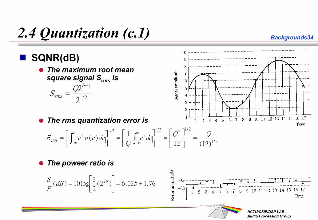
Backgrounds342.4 Quantization (c.1)SQNR(dB)

The maximum root mean square signal Srms is

The rms quantization error is

The poweer ratio is

SQ

rms

b

=−2

2

1

1 2/

E e p e deQ

e deQ Q

rms =

=

=

=

−∞

∞

−∞

∞

∫ ∫21 2

2

1 2 21 2

1 2

1

12 12( )

( )

/ / /

/

S

EdB bb( ) log ( ) . .=

= +10

3

22 6 02 1 762


Backgrounds352.4 Quantization (c.2)Observation

The quantization error is random and perceptually similar to analog white noise for large amplitude signals.Problems– low-amplitude signals.– narrow band signals.

DitherDecorrelates the errors from the signals.Allows the digital system to encode amplitude smaller than the LSB.


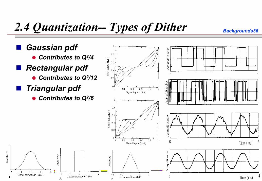
Backgrounds362.4 Quantization-- Types of DitherGaussian pdf

Contributes to Q2/4

Rectangular pdfContributes to Q2/12

Triangular pdfContributes to Q2/6


Backgrounds372.4 Quantization (c.4)Earliest Dither in Word War II

Jim MacArthur has pointed outBombers used mechanical computers to perform navigation and bomb trajectory calculations.These computers perform more accurately when flying on board the aircraft and less well on ground.Engineers realized that the vibration from the aircraft reduced the error from sticky moving parts.


Backgrounds38

Optimal Interpolator:• from Sampling Theorems

• no distortion for the frequency components below Fs/2

• no frequency components above Fs/2 exist and smoothing filtering is not necessary

Suboptimal Interpolator• distortion exists for the frequency

components below Fs/2• result in passing frequencies above

the folding frequency and smoothing filtering is necessary

a an s

x t X n Fs g t nF

( ) ( / ) ( )= −=−∞

∞

∑

Fs 2Fs

F

Signal Mangitude Spectrum

Zero-orderInterpolator

First-orderInterpolator

Optimal Interpolator

2.5 2.5 InterpolatorInterpolator


Backgrounds392.6 Smoothing FiltersDelete the frequency components above a threshold frequency to avoid the image signal introduced bysuboptimal filters

Low-pass filtering

Fc'

Low-Pass Filter

F

1 SmoothingFilter

SmoothingFilter

tt

0 Fs 2Fs2Fs

F

Signal Mangitude Spectrum Cut-off Frequency Fc*


Backgrounds402.7 Concluding RemarksTime/Frequency Illustrarion

Antialiasing filtering and Antiimaging filtering


Backgrounds412.7 Concluding Remarks


Sampling Frequency Fs

t

SmoothingFilter


DigitalSignal

Processing

DigitalSignal

Processing

AnalogOutputSignal

3, 5, 4, 6 ...t

0

t

t3, 5, 4, 6 ...


Cut-off Frequency Fc*

t

AnalogInputSignal

The number of bits

AntialiasingFilter



Backgrounds42Experiment 1WinAmp Architectures

Describe the functionality of Input Plugin, Output Plugin, DSP Plugin, and VIS Plugin.

Find the Input Plugin for Wave File.Change the decoded results for Stereo Channels as

Find the suitable parameters for the two parameters.Describe the noise you have found during the experiments.

][][][][][][][][nLnRnRnRnRnLnLnL

−+=′−+=′

βαβα


Backgrounds43Experiment 2Sampling Rates Change Problem.

1. Change the sampling rates from 44.1kHz to 22.05 kHz by eliminate the odd samples of stereo channels.

L’[n] = L[2n] R’[n] = R[2n]

– Listen to the resulted music and describe the artifacts.– Compare the spectrum through COOL editor to find the spectrum

artifact.2. Change again the sampling rates from 44.1 kHz to 11.025 kHz by three

samples every four samples.L’[n] = L[4n] R’[n] = R[4n]

– Listen to the resulted music and describe the artifacts.– Compare the spectrum through COOL editor to find the spectrum

artifact.


Backgrounds44ExperimentsAnalogInputSignal

Sampling Frequency Fs


t0

ttt

3, 5, 4, 6 ...t

Fc=Fc' and is below 1.5 k ==> Lowpass filtering effectsFc > Fs/2 ==> Aliasing effectsQuantization effectsFs' > Fs or Fs' < Fs ==> Frequency mismatchingFc' > Fs/2 ==> Image effects


Cut-off Frequency

Fc*

The number of bits

AntialiasingFilter

AntialiasingFilte

AnalogOutputSignal

r SamplerSamplerQuantizerQuantizer Smoothing

FilterSmoothing

FilterInterpolatorInterpolator


Backgrounds45

Hearing Area in Frequency Domain

1. Blind Deconvolution for the first music2. Piano Music

a. Original Oneb. Low-pass Onec. Image Distortation (too many high frequency)d. Aliasing effects

Quantization Noise is independent of the Original Signals ?

Documents

Laboratory for Media Processing - National Chiao Tung …people.cs.nctu.edu.tw/~cmliu/Courses/audio/chap1-2.pdfNCTU/CSIE/DSP LAB Audio Processing Group Definition Backgrounds3 Signals