Laboratory Course Polymer Chemistry - Universität … · Give an example of an analytical polymer ... reactions between bifunctional or polyfunctional ... or with the monomeric compound,

Universität Stuttgart

Institute of Polymer Chemistry

Laboratory Course

Polymer Chemistry

Contents:

page

Polymer Analogous Reactions 2

Polycondensation/Polyaddition 8

Radical Polymerization 22

Rheology 49

Polyinsertion and ROMP 70

Emulsion Polymerisation 88

Anionic Polymerization 99

Electropolymerization 107

Viscosimetry 126

Size Exclusion Chromatography 137

DSC 144

- 2 -

POLYMER ANALOGOUS REACTIONS

Assignment of tasks

1. Synthesis of a poly(vinylalcohol) through transesterification reaction of poly(vinyl acetate) using a

methanolic sodium hydroxide solution.

2. Investigations regarding the influence of H-bonding in terms of solubility of poly(vinylalcohol).

Literature

1. D. Braun, H. Cherdron, M. Rehahn, H. Ritter, B. Voit, Polymer Synthesis: Theory and

Practice, 4th Ed., Springer, 2005, page 333, 337.

2. H.-G. Elias, Makromolecules, Band 2, Wiley-VCH, 1. Auflage, 2007, page 276.

Content

1. Introduction

1.1. State of the reacting macromolecule

1.2. Degree of polymerization (end product)

1.2.1. Reactions maintaining the degree of polymerization

1.2.2. Reactions increasing the degree of polymerization

1.2.3. Reactions decreasing the degree of polymerization

1.3. Detail: poly(vinyl alcohol)

2. Experimental procedure

2.1. Safety

2.2. Experiment 1: Poly(vinylalcohol) through transesterification of poly(vinyl acetate)

2.3. Experiment 1: Intermolecular interactions in poly(vinyl acohol)

3. Questions

- 3 -

1 Introduction

Modifications of polymers via chemical reactions are used to modify the polymer and for

investigations regarding composition and constitution.

1.1 State of the reacting macromolecule

The nature of its state and/or its distribution is decisive for a macromolecule in solution for

responding to reactions.

In a good polymer solvent, a reaction of the macromolecule is only discriminable of the same

reaction of a low molecular weight macromolecule if:

1. "neighbouring group effects" are present, e.g., the functional group at the macromolecule is

different with regsards to the constitutional and stereochemical surrounding compared to the

functional group in a low molecular weight macromolecule.

2. side reactions occur. These side reactions, in low molecular chemistry, result in reduced

yields of the isolable main product. Using a macromolecule, chemically different products

result.

3. conversion is <<100%. The resulting macromolecular product is similar to a copolymer

("pseudo-copolymer").

In a poor polymer solvent, due to the high degree of cluster structure, intramolecular ring-closing

reactions occur. If the polymer is insoluble, the only possible reactions are reactions at the surface of

the cluster. If the polymer is swollen in the medium, the rate of reaction depends on the accessibility

of the functional groups in the solvent-swollen regions of the polymer matrix. The situation can

change if the swelling behavior changes or may complicate if insolubility occurs induced by newly

introduced groups. In partially crystalline polymers, reactions only occur in the amorphous regions,

because diffusion procedures are very slow (negligible) in crystalline regions.

1.2 The degree of polymerization of the reacted polymers

Reactions at macromolecules can be divided into three main groups of reactions:

1. reactions while maintaining,

2. while increasing

3. while decreasing the degree of polymerization.

- 4 -

1.2.1 Reactions maintaining the degree of polymerization are called "polymer analogous

reactions". Here, functional groups react in, on or at the end of the polymer chain with other

molecules intermolecularly or intramolecularly within the same chain. Technically important are the

conversion of cellulose to cellulose acetate, cellulose nitrate (collodion, gun cotton, films, coatings)

and cellulose xanthate (viscose). Ion exchange resins and Merrifield resins for peptide synthesis are

obtained by polymer-analogous reaction of functional side groups.

1.2.2 Reactions increasing the degree of polymerization are called “assembly reactions”. They

extend naturally only intermolecularly with functional groups in, on or at the end of the polymer

chain. Reactions in or on the main chain leading to monofunctional agents "graft" to the network

with multi-functional agents. Assembly reactions starting of the end of a polymer chain lead to

"block polymers".

1.2.3 Reactions decreasing the degree of polymerization are called “degradation reactions”.

These are targeted or untargeted reactions occurring chemical, photochemical, thermal or

mechanochemical in nature. These include the chemical and photochemical aging of polymers,

polymer degradation and analytic depolymerization reactions.

1.3 Detail: poly(vinylalcohol)

The saponification or transesterification of poly(vinyl acetate, PVAc) to poly(vinylalcohol, PVA)

represents a typical polymer-analogous reaction of polymer-side selection. Both products can have

the same average degree of polymerization after reaction, the obtained PVA can be re-acetylatet to

default PVAc. Technically, PVA is used for paints, fibers, as emulsifier and in form of protective

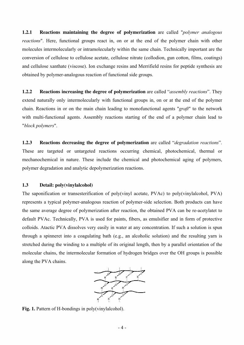
colloids. Atactic PVA dissolves very easily in water at any concentration. If such a solution is spun

through a spinneret into a coagulating bath (e.g., an alcoholic solution) and the resulting yarn is

stretched during the winding to a multiple of its original length, then by a parallel orientation of the

molecular chains, the intermolecular formation of hydrogen bridges over the OH groups is possible

along the PVA chains.

Fig. 1. Pattern of H-bondings in poly(vinylalcohol).

- 5 -

The resulting PVA fiber can no longer be dissolved even in warm water. Only at boiling temperature,

the thermal motion of the macromolecular chains is so strong that the parallel orientation of the

chains is disturbed. The hydrogen bonding between the chains is weakened and in its place water

molecules interact with the OH groups of PVA. The network is released, the molecular chain is

solvated and the PVA string dissolves.

2 Experimental Procedure

2.1 Safety: All persons being exposed to chemicals have to be instructed about the effects of

dangerous substances (toxicity, point of ignition, etc.) as well as about preventive measures. Before

the experiment is carried out, read the MSDS sheets for all of the chemicals used in this laboratory

and be familiar with their safe handling. The instructions of the teaching assistant must be followed

at all times. Especially the following points are relevant:

1. Wearing of suitable protective clothing (protective goggles, glove, laboratory coat, etc.)

2. Knowledge about the safety devices (e.g., laboratory hood, fire extinguisher, emergency

shower, first aid boxes, etc.) and exit.

3. Controlled disposal of toxic compounds in compliance with legal regulations.

4. Strict ban on eating/drinking/smoling in the laboratory.

2.2 Experiment 1: Poly(vinylalcohol) through transesterification of poly(vinyl acetate)

Chemicals: 25 mL methanolic NaOH-solution (1 wt.-%)

7.5 g poly(vinyl acetate, PVAc)

methanol, chloroform, tetrahydrofuran (THF), dimethyl formamide (DMF),

toluene, acetone

Equipment: 250-mL 3-neck flask

stirrer, stirring engine

reflux condenser

100-mL-dropping funnel with pressure balance

water bath, thermometer, porcelain suction filter

test tubes, glass rods, funnels

100 mL graduated cylinder

Procedure:

In a 250 mL three-necked flask with stirrer, reflux condenser and dropping funnel 25 mL of a l wt.-%

methanolic sodium hydroxide solution is heated in a water bath up to 50 °C. Under vigorous stirring

- 6 -

within 30 minutes, a solution of 7.5 g of PVAc in 80 mL of methanol is added dropwise. The

transesterification can be seen at the onset of the precipitation of PVA. After addition is complete,

stirring is continued for another 30 minutes, then the precipitate is filtered off, washed with methanol

and dried in vacuo free of alkali. The solubility of PVA is compared in test tubes with various cold

and warm (water bath!) organic solvents (methanol, chloroform, THF, DMF, toluene and acetone)

and in cold and warm water with the solubility of PVAc. Comment on the log of your observations.

With a solvent mixture of methanol / water 30/70, a 10 wt.-% PVA solution is prepared. This

solution is spread with a glass rod on a glass plate. After careful prolonged drying in an oven (PVA

is slightly hygroscopic!), a polymer film can be removed. Of these, an IR spectrum is made that you

should compare with an IR spectrum of PVAc provided.

2.3 Experiment 2: intermolecular interactions in PVA

Chemicals: different fibers made of poly(vinylalcohol)

dionized H2O

Equipment: 600 mL beaker, high form

piece weight

heating plate

thermometers

Procedure:

In an manual experiment, the solubility of three different PVA filaments under tension is

investigated. For this purpose, on each yarn made of PVA fibres a weight of about 100 g is attached

and slowly lowered into a beaker with water. Starting with yarn 1, the influence of the bath

temperature is examined for the solubility behavior. For examination, the water is slowly heated and

the dissolving of the respective threads is observed. What is observed, as long as the weight piece

hangs freely and is placed on the bottom of the cup-glass? Explain the observed behavior in the

protocol.

- 7 -

3 Question

1. What is the equation for the formation of PVAc?

2. Why can PVA not be produced by direct polymerization of the corresponding monomers?

3. Formulate the polymer-analogous reaction of PVA with aldehydes. Why are there no

networking products?

4. Give an example of an analytical polymer degradation and chemical aging of polymers.

- 8 -

POLYCONDENSATION and POLYADDITION

I Polycondensation

Assignment of tasks

1. Investigation of polycondensation kinetics via the reaction of succinic acid and 1,6-

hexandiol: In the acid-catalyzed polycondensation, the change of the carboxyl group‘s

concentration should be presented as a function of time. Further, the rate constant for this

condensation reaction should be determined.

2. Nylon-6, 10 thread should be made by the interfacial polycondensation of sebacoyl chloride

in cyclohexane and 1,6-hexamethylenediamine in water.

Literature


Practice, 4th Ed., Springer, 2005.

2. H.-G. Elias, Makromolecules Bd. 1, 1. Auflage, Wiley-VCH-Verlag, Weinheim, 2005.

3. P. J. Flory, J. Am. Chem. Soc. (1939), 61, 3334

Content

1. Introduction

1.1. Reactions by using different kinds of starting compounds with identical end groups

1.2. Reactions by using the same starting compounds with identical end groups


2.1. Safety

2.2. Experimental proceduce

2.3. Evaluation

2.4. Hands on experiment

3. Questions

- 9 -

1 Introduction

Condensation polymerizations are stepwise reactions between bifunctional or polyfunctional

components that entail the elimination of small molecules such as water, HCl, NaCl, NH3, HCN,

CH3OH etc. and the formation of macromolecular substances (step growth polymerization). For the

preparation of linear condensation polymers from bifunctional compounds, there are basically two

possibilities. One either starts from a monomer, which has two different groups suitable for

polycondensation (AB type), or one starts from two different monomers, each possessing a pair of

identical reactive groups that can reaction with each other (AA-BB type).

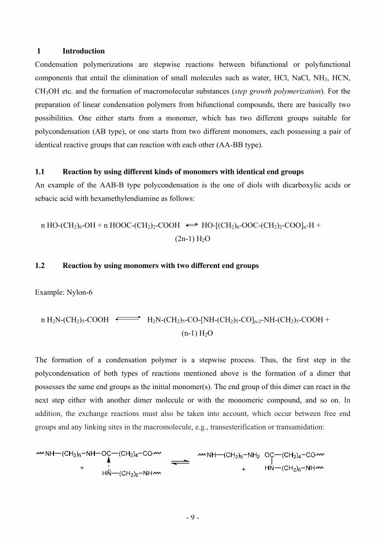
1.1 Reaction by using different kinds of monomers with identical end groups

An example of the AAB-B type polycondensation is the one of diols with dicarboxylic acids or

sebacic acid with hexamethylendiamine as follows:

n HO-(CH2)6-OH + n HOOC-(CH2)2-COOH HO-[(CH2)6-OOC-(CH2)2-COO]n-H +

(2n-1) H2O

1.2 Reaction by using monomers with two different end groups

Example: Nylon-6

n H2N-(CH2)5-COOH H2N-(CH2)5-CO-[NH-(CH2)5-CO]n-2-NH-(CH2)5-COOH +

(n-1) H2O

The formation of a condensation polymer is a stepwise process. Thus, the first step in the

polycondensation of both types of reactions mentioned above is the formation of a dimer that

possesses the same end groups as the initial monomer(s). The end group of this dimer can react in the

next step either with another dimer molecule or with the monomeric compound, and so on. In

addition, the exchange reactions must also be taken into account, which occur between free end

groups and any linking sites in the macromolecule, e.g., transesterification or transamidation:

- 10 -

In the polycondensation, the monomers, linear and cyclic oligomers and polymers are always in

equilibrium. However, the content of cyclic oligomers decreases with increasing molecular weight.

In contrast to chain growth polymerization, in which the polymerizations are typical chain-reactions

involving a starting step (initiation) followed by many identical chain-reaction steps (propagation),

each condensation step needs to be activated and requires the same activation energy.

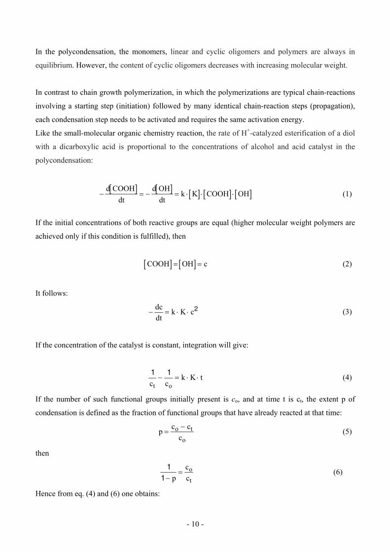
Like the small-molecular organic chemistry reaction, the rate of H+-catalyzed esterification of a diol

with a dicarboxylic acid is proportional to the concentrations of alcohol and acid catalyst in the

polycondensation:

d COOH

dt

d OH

dtk K COOH OH (1)

If the initial concentrations of both reactive groups are equal (higher molecular weight polymers are

achieved only if this condition is fulfilled), then

COOH OH c (2)

It follows:

dc

dtk K c2 (3)

If the concentration of the catalyst is constant, integration will give:

1 1

c ck K t

t o (4)

If the number of such functional groups initially present is co, and at time t is ct, the extent p of

condensation is defined as the fraction of functional groups that have already reacted at that time:

pc c

co t

o

(5)

then

1

1

p

c

co

t (6)

Hence from eq. (4) and (6) one obtains:

- 11 -

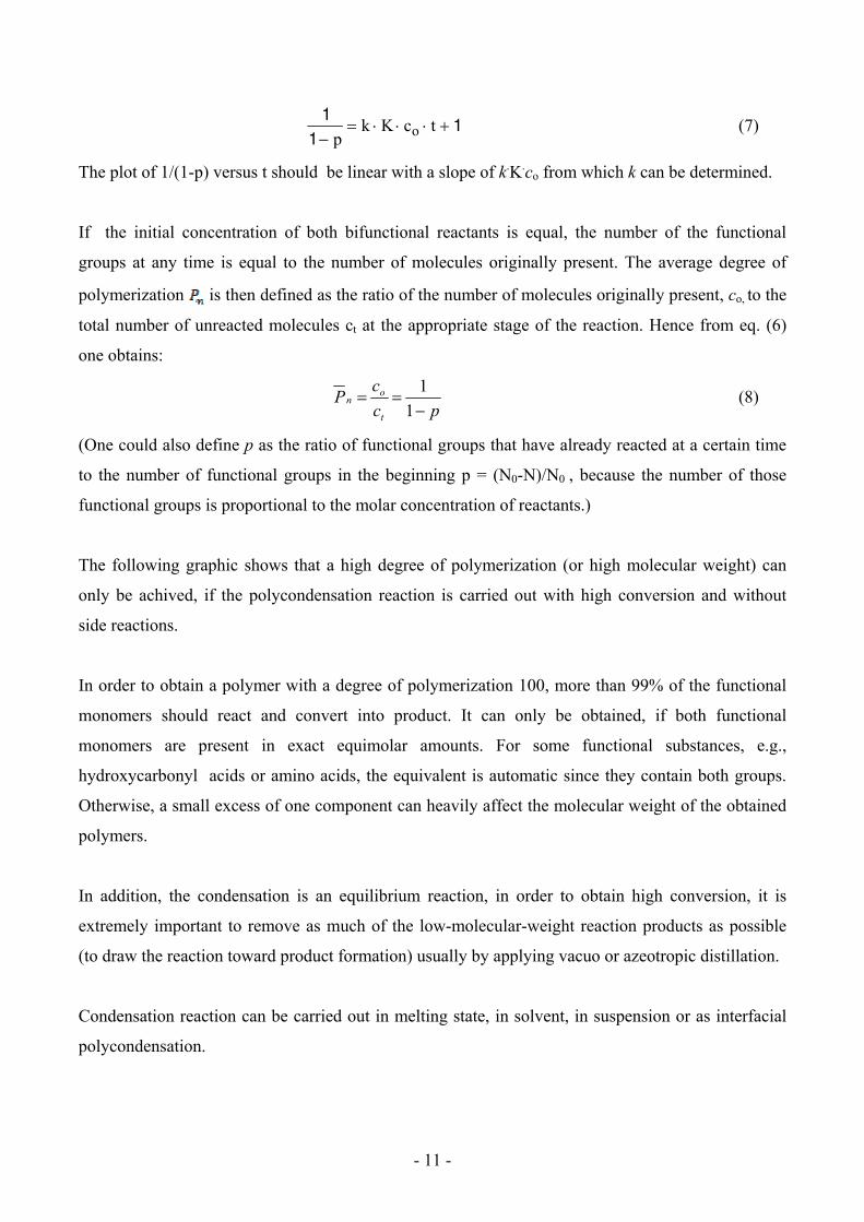
1

11

pk K c to (7)

The plot of 1/(1-p) versus t should be linear with a slope of k.K.co from which k can be determined.

If the initial concentration of both bifunctional reactants is equal, the number of the functional

groups at any time is equal to the number of molecules originally present. The average degree of

polymerization is then defined as the ratio of the number of molecules originally present, co, to the

total number of unreacted molecules ct at the appropriate stage of the reaction. Hence from eq. (6)

one obtains:

pc

cP

t

on

1

1 (8)

(One could also define p as the ratio of functional groups that have already reacted at a certain time

to the number of functional groups in the beginning p = (N0-N)/N0 , because the number of those

functional groups is proportional to the molar concentration of reactants.)

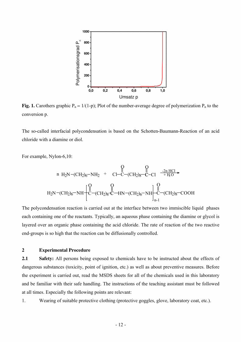
The following graphic shows that a high degree of polymerization (or high molecular weight) can

only be achived, if the polycondensation reaction is carried out with high conversion and without

side reactions.

In order to obtain a polymer with a degree of polymerization 100, more than 99% of the functional

monomers should react and convert into product. It can only be obtained, if both functional

monomers are present in exact equimolar amounts. For some functional substances, e.g.,

hydroxycarbonyl acids or amino acids, the equivalent is automatic since they contain both groups.

Otherwise, a small excess of one component can heavily affect the molecular weight of the obtained

polymers.

In addition, the condensation is an equilibrium reaction, in order to obtain high conversion, it is

extremely important to remove as much of the low-molecular-weight reaction products as possible

(to draw the reaction toward product formation) usually by applying vacuo or azeotropic distillation.

Condensation reaction can be carried out in melting state, in solvent, in suspension or as interfacial

polycondensation.

- 12 -

0,0 0,2 0,4 0,6 0,8 1,00

200

400

600

800

1000

Poly

merisationsgra

d P

n

Umsatz p

Fig. 1. Carothers graphic Pn 1/(1-p); Plot of the number-average degree of polymerization Pn to the

conversion p.

The so-called interfacial polycondensation is based on the Schotten-Baumann-Reaction of an acid

chloride with a diamine or diol.

For example, Nylon-6,10:

n-1

HN (CH2)6 NH

O

C (CH2)8 COOHC (CH2)8 C

O

C

O

H2N (CH2)6 NH

2+ H O -2n HCl

O

C

O

+H2N (CH2)6 NH2n C ClC (CH2)8Cl

The polycondensation reaction is carried out at the interface between two immiscible liquid phases

each containing one of the reactants. Typically, an aqueous phase containing the diamine or glycol is

layered over an organic phase containing the acid chloride. The rate of reaction of the two reactive

end-groups is so high that the reaction can be diffusionally controlled.

2 Experimental Procedure






1. Wearing of suitable protective clothing (protective goggles, glove, laboratory coat, etc.).

- 13 -


shower, first aid boxes, etc.), exit.

3. Controlled disposal of toxic substances in compliance with legal regulations.

4. Strict ban on eating, drinking, smoking in the laboratory.

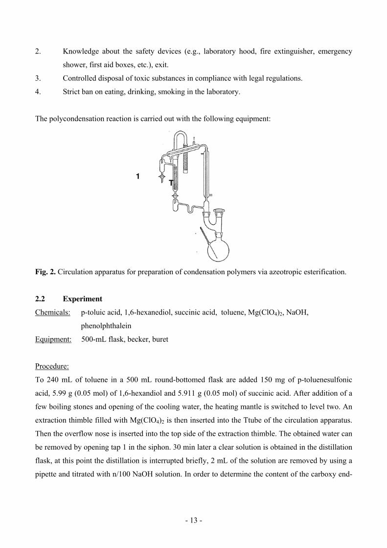
The polycondensation reaction is carried out with the following equipment:

Fig. 2. Circulation apparatus for preparation of condensation polymers via azeotropic esterification.

2.2 Experiment

Chemicals: p-toluic acid, 1,6-hexanediol, succinic acid, toluene, Mg(ClO4)2, NaOH,

phenolphthalein

Equipment: 500-mL flask, becker, buret

Procedure:

To 240 mL of toluene in a 500 mL round-bottomed flask are added 150 mg of p-toluenesulfonic

acid, 5.99 g (0.05 mol) of 1,6-hexandiol and 5.911 g (0.05 mol) of succinic acid. After addition of a

few boiling stones and opening of the cooling water, the heating mantle is switched to level two. An

extraction thimble filled with Mg(ClO4)2 is then inserted into the Ttube of the circulation apparatus.

Then the overflow nose is inserted into the top side of the extraction thimble. The obtained water can

be removed by opening tap 1 in the siphon. 30 min later a clear solution is obtained in the distillation

flask, at this point the distillation is interrupted briefly, 2 mL of the solution are removed by using a

pipette and titrated with n/100 NaOH solution. In order to determine the content of the carboxy end-

1 T

- 14 -

group, aiddtional samples will be taken at intervals of 30 min for a total reaction time of 5~6 hours

and then titrated with the above-mentioned NaOH solution.

2.3 Evaluation

After the beginning of the cycle there are exactly 100 mL of solution in the distillation flask.

Statistically every condensated molecule contains an average of one alcohol and one carboxyl end

group. From the consumption of n/100 NaOH solution the number of mole of carboxyl end groups

can be calculated. This number is plotted against time. By using equation (5) the validity of the

correlation in equation (7) is verified.

2.4 Hands on experiment

Synthesis of nylon-6, 10 via the interfacial polycondensation

Chemicals: 3 mL sebacoyl chloride

4,4 g hexamethylendiamine

100 mL cyclohexane

50 mL dist. water

sodium hydrogencarbonate, acetone,

phenolphthalein

Equiments: beakers (1x200 mL, 2x400 mL)

measuring zylinder (1x50 mL, 1x100 mL)

pipette 3 mL

stirrer, glas bar, glas funnel

A solution of 4.4 g (26 mmol) of hexamethylene diamine in 50 mL of water in a beaker is carefully

layered with a solution of 3 mL (14 mmol) of sebacic acid dichloride in 100 mL of cyclohexane by

means of a funnel. For a besser visualization of the separated phase a small amount of

phenolphthalein can be added into the aqueous solution. A thin film will form at the interface. Draw

a thread out of the interface by using a tweezer and place it on the glass rod in the stirrer motor. After

switching on the motor a fiber can be extracted continuously. The product is washed in a 400 mL

beaker first with sodium bicarbonate solution, then with water and finally with acetone and

eventually dried in a vacuum oven at 60 °C.

- 15 -

3 Questions

1. What kind of correlation of conversion p and reaction time t do you expect in case of the

auto-catalyzed polycondensation of a dicarboxylic acid and a diol? How can this be

demonstrated experimentally?

2. In principle what kind of possibilities are there to regulate the molecular weight of a

polycondensate and what has to be kept in mind regarding the end groups?

3. You are supposed to synthesize a polycondensate with a dicarboxylic acid and ethylene

glycol (Kp(760) = 198 oC). What difficulties do you expect when using an azeotropic

esterification and applying toluene Kp(760) = 110,6 oC) as hauler? How can this difficulty

be bypassed?

4. What kind of methods for the synthesis of polyamides do you know?

- 16 -

II Polyaddition

Assignment of tasks

Synthesis of polyurethane through a polyaddition reaction between a polyole and a diisocyanate.

Literature:

1. J. H. Saunders, W. Frisch, “Polyurethanes: Chemistry and Technology I: Chemistry”, in

“High Polymers” XVI, 1962, S. 63.

2. G. Oertel, Kunststoffbuch Bd. 7, Polyurethane, Hanser Verlag München 1983.


Practice, 4th Ed., Springer, 2005, page 333, 337.

4. H.-G. Elias, Makromolecules, Bd. 1, 1. Auflage, Wiley‐VCH‐Verlag, Weinheim, 2005.

Content

1. Introduction

2. Mechanism

2.1. Reaction in the absence of a catalyst

2.2. Reaction in the presence of a catalyst


3.1. Safety

3.2. Experiment

4. Questions

- 17 -

1 Introduction

The formation of synthetic polymers is a process, which occurs via chemical connection of many

hundreds up to many thousands of monomer molecules. As a result, macromolecular chains are

formed. They are, in general, linear, but can be branched, or crosslinked as well. The chemical

process of chain formation may be divided into two classes, depending on whether it proceeds as a

chain-growth or as a step-growth reaction. Condensation polymerizations (or step-growth

polymerization) comprise of the stepwise reaction between bifunctional or polyfunctional

components, with elimination of small molecules such as water, alcohol, or hydrogen and the

formation of macromolecular substances. Polymers such as polyamides and polyesters can be

prepared via condensation polymerization; this type of condensation polymerization is therefore

termed polycondensation. In contrast to condensation polymerization, addition polymerization (also

called polyaddition) involves a stepwise reaction of at least two bifunctional components, leading to

the formation of macromolecules; however, in course of this process no low-molecular-weight

compounds are eliminated. The coupling of the monomer units is a consequence of the migration of

a hydrogen atom. Like condensation polymerization, this kind of addition polymerization is also a

stepwise reaction, consisting of a sequence of independent individual reactions, so that the average

molecular weight of the resulting polymer steadily increases during the course of the reaction. The

oligomeric and polymeric products formed in the individual steps possess the same functional end

groups and the same reactivity as the starting materials; they can be isolated without losing their

reactivity. As all stepwise reactions, they are also governed by kinetic laws similar to those for

condensation polymerization.

The classical and important stepwise addition polymerization is the reaction of the di- or

polyfunctional isocyanate with di- or polyfunctional hydroxy compounds, or other compounds

having a plurality of active hydrogen atoms, to form the macromolecules in which the constitutional

repeating units are coupled with one another via urethane or urea groups (scheme 1).

Scheme 1. Polyurethane and polyurea formation.

- 18 -

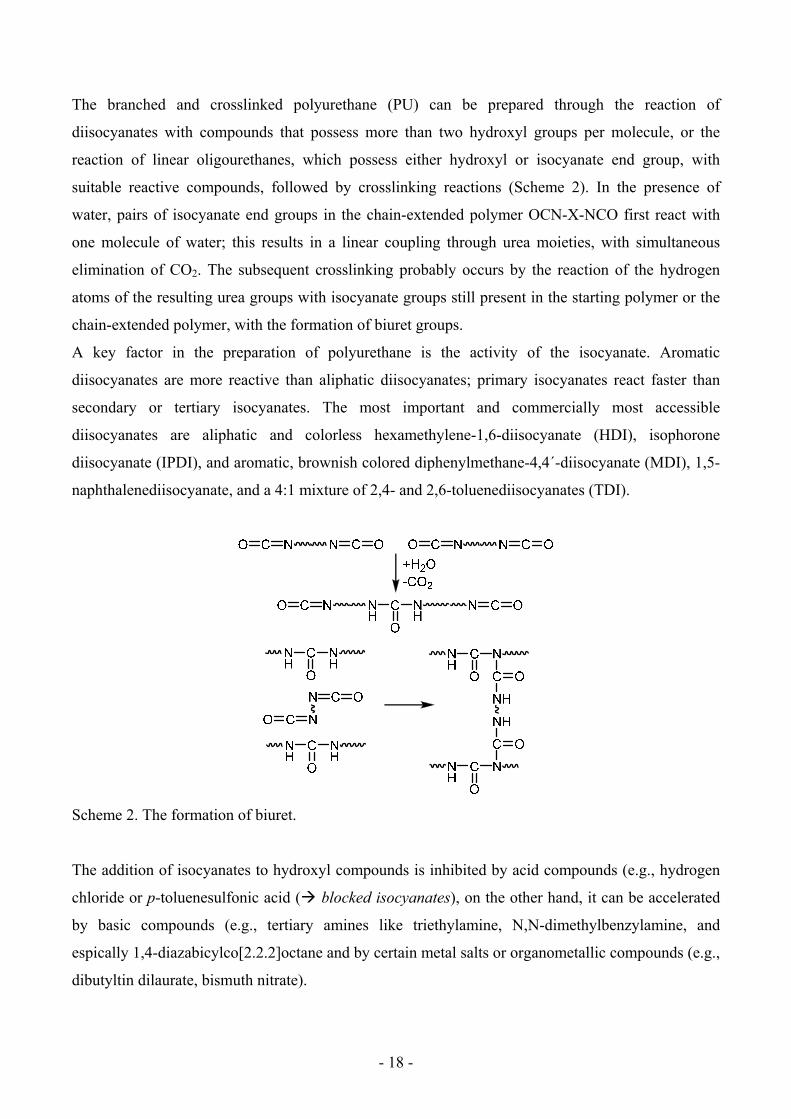
The branched and crosslinked polyurethane (PU) can be prepared through the reaction of

diisocyanates with compounds that possess more than two hydroxyl groups per molecule, or the

reaction of linear oligourethanes, which possess either hydroxyl or isocyanate end group, with

suitable reactive compounds, followed by crosslinking reactions (Scheme 2). In the presence of

water, pairs of isocyanate end groups in the chain-extended polymer OCN-X-NCO first react with

one molecule of water; this results in a linear coupling through urea moieties, with simultaneous

elimination of CO2. The subsequent crosslinking probably occurs by the reaction of the hydrogen

atoms of the resulting urea groups with isocyanate groups still present in the starting polymer or the

chain-extended polymer, with the formation of biuret groups.

A key factor in the preparation of polyurethane is the activity of the isocyanate. Aromatic

diisocyanates are more reactive than aliphatic diisocyanates; primary isocyanates react faster than

secondary or tertiary isocyanates. The most important and commercially most accessible

diisocyanates are aliphatic and colorless hexamethylene-1,6-diisocyanate (HDI), isophorone

diisocyanate (IPDI), and aromatic, brownish colored diphenylmethane-4,4´-diisocyanate (MDI), 1,5-

naphthalenediisocyanate, and a 4:1 mixture of 2,4- and 2,6-toluenediisocyanates (TDI).

Scheme 2. The formation of biuret.

The addition of isocyanates to hydroxyl compounds is inhibited by acid compounds (e.g., hydrogen

chloride or p-toluenesulfonic acid ( blocked isocyanates), on the other hand, it can be accelerated

by basic compounds (e.g., tertiary amines like triethylamine, N,N-dimethylbenzylamine, and

espically 1,4-diazabicylco[2.2.2]octane and by certain metal salts or organometallic compounds (e.g.,

dibutyltin dilaurate, bismuth nitrate).

- 19 -

2 Mechanism

The reaction of an isocyanate with an active hydrogen compounds is carried out with or without a

catalyst. The self-addition reactions of isocyanates do usually not proceed as readily as reactions

with active hydrogen compounds.

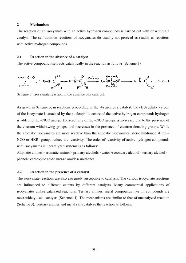
2.1 Reaction in the absence of a catalyst

The active compound itself acts catalytically in the reaction as follows (Scheme 3).

Scheme 3. Isocyanate reaction in the absence of a catalyst.

As given in Scheme 3, in reactions proceeding in the absence of a catalyst, the electrophilic carbon

of the isocyanate is attacked by the nucleophilic centre of the active hydrogen compound; hydrogen

is added to the –NCO group. The reactivity of the –NCO groups is increased due to the presence of

the electron withdrawing groups, and decreases in the presence of electron donating groups. While

the aromatic isocyanates are more reactive than the aliphatic isocyanates, steric hindrance at the –

NCO or HXR’ groups reduce the reactivity. The order of reactivity of active hydrogen compounds

with isocyanates in uncatalyzed systems is as follows:

Aliphatic amines> aromatic amines> primary alcohols> water>secondary alcohol> tertiary alcohol>

phenol> carboxylic acid> ureas> amides>urethanes.

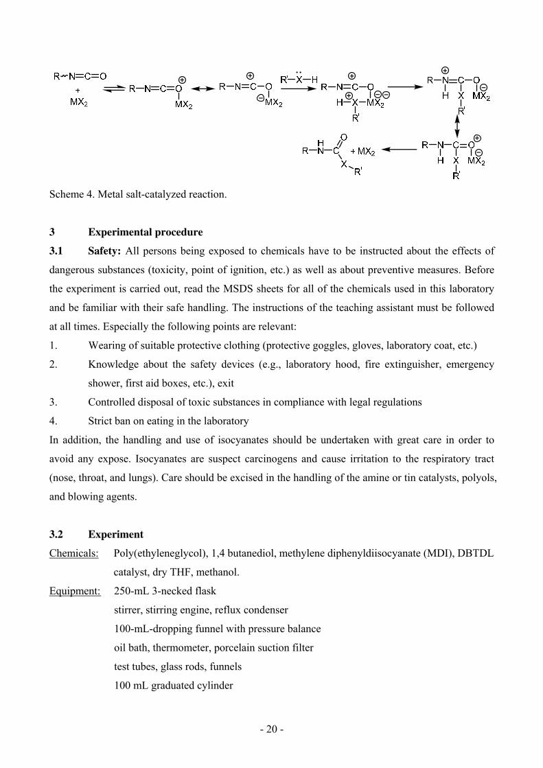
2.2 Reaction in the presence of a catalyst

The isocyanate reactions are also extremely susceptible to catalysis. The various isocyanate reactions

are influenced to different extents by different catalysts. Many commercial applications of

isocyanates utilize catalyzed reactions. Tertiary amines, metal compounds like tin compounds are

most widely used catalysts (Schemes 4). The mechanisms are similar to that of uncatalyzed reaction

(Scheme 3). Tertiary amines and metal salts catalyze the reaction as follows:

- 20 -

Scheme 4. Metal salt-catalyzed reaction.

3 Experimental procedure






1. Wearing of suitable protective clothing (protective goggles, gloves, laboratory coat, etc.)


shower, first aid boxes, etc.), exit

3. Controlled disposal of toxic substances in compliance with legal regulations

4. Strict ban on eating in the laboratory

In addition, the handling and use of isocyanates should be undertaken with great care in order to

avoid any expose. Isocyanates are suspect carcinogens and cause irritation to the respiratory tract

(nose, throat, and lungs). Care should be excised in the handling of the amine or tin catalysts, polyols,

and blowing agents.

3.2 Experiment

Chemicals: Poly(ethyleneglycol), 1,4 butanediol, methylene diphenyldiisocyanate (MDI), DBTDL

catalyst, dry THF, methanol.

Equipment: 250-mL 3-necked flask

stirrer, stirring engine, reflux condenser

100-mL-dropping funnel with pressure balance

oil bath, thermometer, porcelain suction filter

test tubes, glass rods, funnels

100 mL graduated cylinder

- 21 -

Procedure:

Before starting the reaction, all monomers such as the macro-diol or 1,4-butanediol (BD) need to be

well dried in vacuo with appropriate temperature for removing residual moisture. The reaction is to

be performed by solution polymerization.

In a typical reaction, 1 equivalent of the macro-diol (3.0 g, 2.0 mmol ) and 2.2 equivalents of MDI (

1.1 g, 4.4 mmol) are mixed with 20mL of dry THF and taken in a dry 3 necked RB under dry

nitrogen atmosphere. Then the RB is placed on a magnetic stirrer and heated at 60°C. After complete

mixing of all monomers, 0.01% (0.003 g) of DBTDL catalyst (based on the weight of macro-diol ) is

added. 2 h later, 2 equivalents of 1,4 butanediol (0.1802 g, 2 mmol) are added and the mixture is

stirred again for 3-4 hr at reflux. The final mixture is then purified by precipitating the polymer from

methanol followed by repeated washings for removal of any unreacted monomer. The precipitate is

then dried in a vacuum oven at 60°C for 24 hrs.

4 Questions:

1. Formulate the reaction mechanism of the obtained polyurethane using a base as catalyst.

2. Why are neither primary nor secondary amines used as catalysts for the synthesis of

polyurethanes?

3. Why are low boiling tertiary amines not used as catalysts?

4. Formulate the equation for the formation of urea from the prepolymer containing isocyanate

groups and water.

5. Formulate the crosslinking equation with the formation of a biuret structure from the

starting polymer or the chain-extended polymer containing isocyanate groups in the

presence of water.

6. What will happen if the reaction of isocyanate and water is faster then the reaction of

isocyanate with polyol, and vice versa?

7. What are the side reactions occurring if some moisture is present in the reaction system?

- 22 -

RADICAL POLYMERIZATION

Literature

1. H. G. Elias, Bd. 1, 1. Auflage, Wiley-VCH-Verlag, Weinheim, 2005.

2. G. Odian, “Principles of Polymerization”, John Wiley & Sons, Inc., 3rd Ed., New York 1991, S. 198 ff

3. F. R. Mayo, F. M. Lewis, J. Am. Chem. Soc. (1944), 66, 1594

4. M. Fineman, S. D. Ross, J. Polym. Sci. (1959), 5, 259

Content

1. Introduction

2. General overview over the reaction mechanism

2.1. Initiation

2.2. Propagation

2.3. Termination

2.4. Dependence of the degree of polymerization on conversion

2.5. Reaction scheme and kinetics

3. Experimental verification of the rate law

3.1. Determination of the total rate

3.2. Dependence of the total rate on the concentration of the starting materials

4. Other concepts in the free-radical polymerization

4.1. Kinetic chain length and degree of polymerization

4.2. Chain transfer

4.3. The Trommsdorff-effect

5. Radical copolymerization

5.1. Copolymerization equation

5.2. Influence of the penultimate incorporated monomers on propagation

5.3. Discussion of the r1, r2 values

5.4. Experimental determination of the copolymerization parameters

5.5. Influence of the monomers constitution on the copolymerization parameters

6. Statistic of the polymer chain

6.1. Sequence distribution in copolymer

6.2. Calculation of the average sequence length ( I1 )

6.3. Definition and calculation of the run number ®


8. Questions

- 23 -

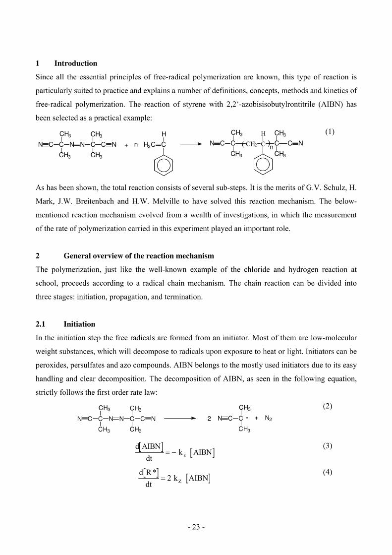
1 Introduction

Since all the essential principles of free-radical polymerization are known, this type of reaction is

particularly suited to practice and explains a number of definitions, concepts, methods and kinetics of

free-radical polymerization. The reaction of styrene with 2,2‘-azobisisobutylrontitrile (AIBN) has

been selected as a practical example:

n)(N C C

CH3

CH3

CH2 C

H

N

CH3

CH3

CCn H2C C

H

+N C C

CH3

CH3

N N C C

CH3

CH3

N

(1)

As has been shown, the total reaction consists of several sub-steps. It is the merits of G.V. Schulz, H.

Mark, J.W. Breitenbach and H.W. Melville to have solved this reaction mechanism. The below-

mentioned reaction mechanism evolved from a wealth of investigations, in which the measurement

of the rate of polymerization carried in this experiment played an important role.

2 General overview of the reaction mechanism

The polymerization, just like the well-known example of the chloride and hydrogen reaction at

school, proceeds according to a radical chain mechanism. The chain reaction can be divided into

three stages: initiation, propagation, and termination.

2.1 Initiation

In the initiation step the free radicals are formed from an initiator. Most of them are low-molecular

weight substances, which will decompose to radicals upon exposure to heat or light. Initiators can be

peroxides, persulfates and azo compounds. AIBN belongs to the mostly used initiators due to its easy

handling and clear decomposition. The decomposition of AIBN, as seen in the following equation,

strictly follows the first order rate law:

N2+2 N C C

CH3

CH3

N C C

CH3

CH3

N N C C

CH3

CH3

N

(2)

d AIBN

dt k AIBNz

(3)

d R *

dt2 k AIBNz

(4)

- 24 -

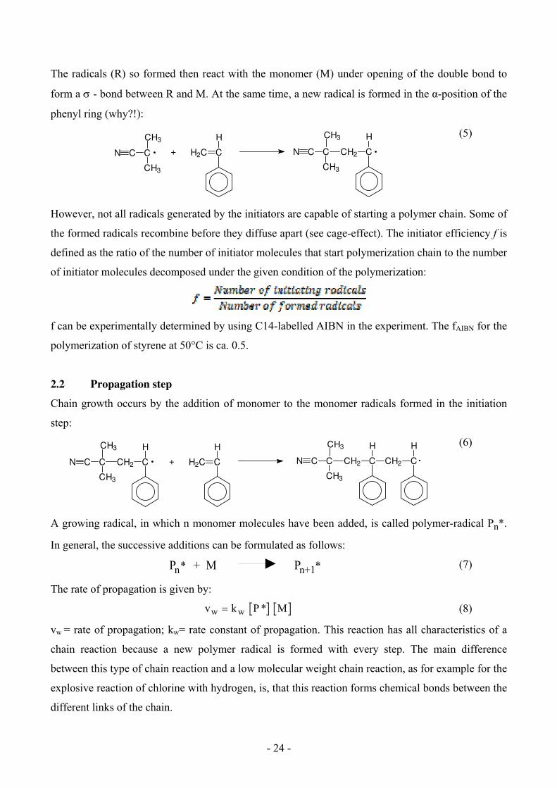
The radicals (R) so formed then react with the monomer (M) under opening of the double bond to

form a - bond between R and M. At the same time, a new radical is formed in the α-position of the

phenyl ring (why?!):

+N C C

CH3

CH3

H2C C

H

N C C

CH3

CH3

CH2 C

H

(5)

However, not all radicals generated by the initiators are capable of starting a polymer chain. Some of

the formed radicals recombine before they diffuse apart (see cage-effect). The initiator efficiency f is

defined as the ratio of the number of initiator molecules that start polymerization chain to the number

of initiator molecules decomposed under the given condition of the polymerization:

f can be experimentally determined by using C14-labelled AIBN in the experiment. The fAIBN for the

polymerization of styrene at 50°C is ca. 0.5.

2.2 Propagation step

Chain growth occurs by the addition of monomer to the monomer radicals formed in the initiation

step:

N C C

CH3

CH3

CH2 C

H H

CCH2N C C

CH3

CH3

CH2 C

H

+ H2C C

H

(6)

A growing radical, in which n monomer molecules have been added, is called polymer-radical Pn*.

In general, the successive additions can be formulated as follows:

Pn + M Pn+1* *

(7)

The rate of propagation is given by:

v k P * Mw w (8)

vw = rate of propagation; kw= rate constant of propagation. This reaction has all characteristics of a

chain reaction because a new polymer radical is formed with every step. The main difference

between this type of chain reaction and a low molecular weight chain reaction, as for example for the

explosive reaction of chlorine with hydrogen, is, that this reaction forms chemical bonds between the

different links of the chain.

- 25 -

2.3 Termination

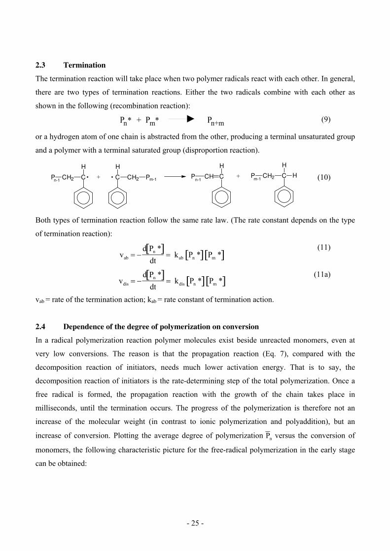
The termination reaction will take place when two polymer radicals react with each other. In general,

there are two types of termination reactions. Either the two radicals combine with each other as

shown in the following (recombination reaction):

Pn + P Pn+mm* *

(9)

or a hydrogen atom of one chain is abstracted from the other, producing a terminal unsaturated group

and a polymer with a terminal saturated group (disproportion reaction).

P CH2 C

H

n-1+ PCH2C

H

m-1P CH C

H

n-1P CH2 C

H

Hm-1

+

(10)

Both types of termination reaction follow the same rate law. (The rate constant depends on the type

of termination reaction):

vab d Pn *

dt kab Pn * Pm *

vdis d Pn *

dt kdis Pn * Pm *

(11)

(11a)

vab = rate of the termination action; kab = rate constant of termination action.

2.4 Dependence of the degree of polymerization on conversion

In a radical polymerization reaction polymer molecules exist beside unreacted monomers, even at

very low conversions. The reason is that the propagation reaction (Eq. 7), compared with the

decomposition reaction of initiators, needs much lower activation energy. That is to say, the

decomposition reaction of initiators is the rate-determining step of the total polymerization. Once a

free radical is formed, the propagation reaction with the growth of the chain takes place in

milliseconds, until the termination occurs. The progress of the polymerization is therefore not an

increase of the molecular weight (in contrast to ionic polymerization and polyaddition), but an

increase of conversion. Plotting the average degree of polymerization Pn versus the conversion of

monomers, the following characteristic picture for the free-radical polymerization in the early stage

can be obtained:

- 26 -

Fig. 1: Dependence of the degree of polymerization on conversion for the radical polymerization.

2.5 Reaction scheme and kinetics

The rate law for the total reaction can be determined from the partial reaction and its rate law. The

total rate vBr is defined as the conversion of monomer to polymer per unit volume and per unit time:

vd M

dt

M

tBr

(12)

For clarity, all of the individual reactions are combined in a reaction scheme:

initiation:

AIBN k z

2 f R*

R* + M k st

P1*

propagation:

P1* + M k w1

P2*

P2* + M k w2

P3*

Pn-1* + M k wn-1

Pn*

termination:

Pn* + Pm* k ab

Pn+m

oder k ab

Pn + Pm

The kinetics of the ideal polymerization can then be derived with the help of the reaction scheme. In

order to be successful, we need the following assumptions:

- 27 -

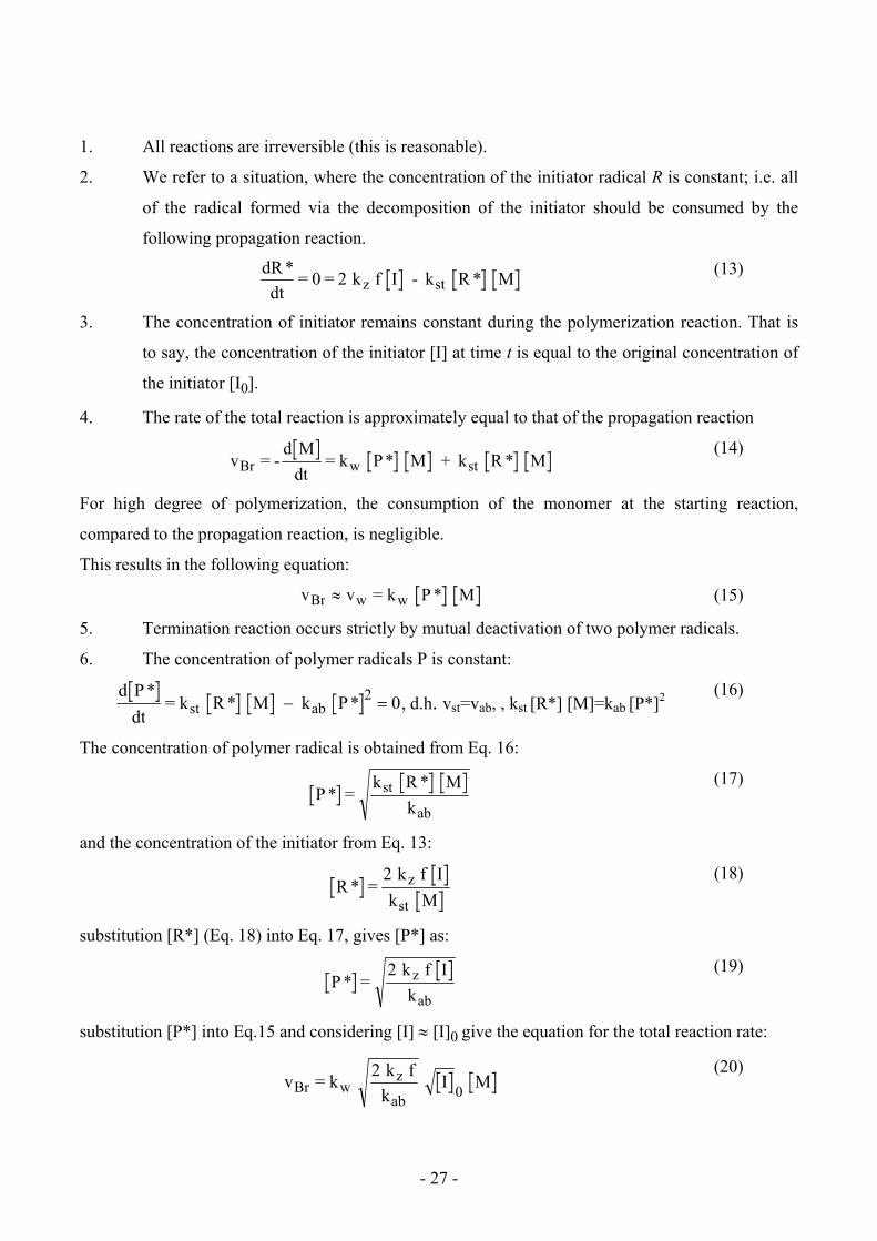
1. All reactions are irreversible (this is reasonable).

2. We refer to a situation, where the concentration of the initiator radical R is constant; i.e. all

of the radical formed via the decomposition of the initiator should be consumed by the

following propagation reaction.

dR *

dt= 0 = 2 k f I - k R * Mz st

(13)

3. The concentration of initiator remains constant during the polymerization reaction. That is

to say, the concentration of the initiator [I] at time t is equal to the original concentration of

the initiator [I0].

4. The rate of the total reaction is approximately equal to that of the propagation reaction

v = -d M

dt= k P* M + k R * MBr w st

(14)

For high degree of polymerization, the consumption of the monomer at the starting reaction,

compared to the propagation reaction, is negligible.

This results in the following equation:

v v = k P * MBr w w (15)

5. Termination reaction occurs strictly by mutual deactivation of two polymer radicals.

6. The concentration of polymer radicals P is constant:

d P*

dt= k R * M k P*st ab

2 0, d.h. vst=vab, , kst [R*] [M]=kab [P*]2 (16)

The concentration of polymer radical is obtained from Eq. 16:

P * =k R * M

kst

ab

(17)

and the concentration of the initiator from Eq. 13:

R * =2 k f I

k Mz

st

(18)

substitution [R*] (Eq. 18) into Eq. 17, gives [P*] as:

P * =2 k f I

kz

ab

(19)

substitution [P*] into Eq.15 and considering [I] [I]0 give the equation for the total reaction rate:

v = k 2 k f

k I MBr w

z

ab0

(20)

- 28 -

3 The experimental verification of the rate law

3.1 Determination of the total rate

According to eq. 12, the total reaction rate or the rate of polymerization is defined as negative time

dependent change in the monomer concentration. All physical and chemical properties that will be

changed during the polymerization can be used for determining this change. One of the most

applicable methods is the dilatometric method. Its principal is based on the change of the specific

volume in the transition state of monomer to polymer. The term “dilatometry” is somehow

misleading, as the polymer has a higher density than the monomer and, therefore, only a contraction

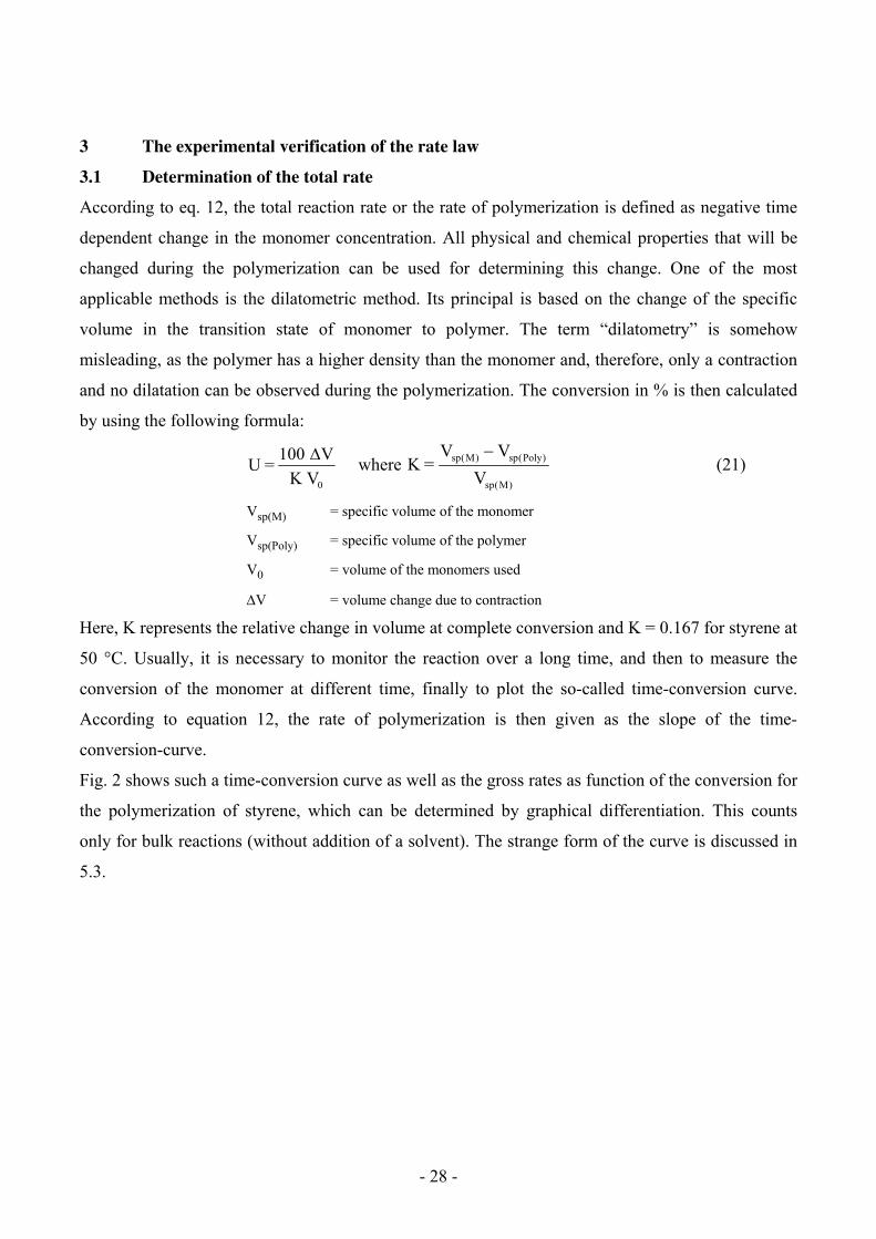
and no dilatation can be observed during the polymerization. The conversion in % is then calculated

by using the following formula:

U =100 V

K V0

where K =

V V

Vsp(M) sp(Poly)

sp(M)

(21)

Vsp(M) = specific volume of the monomer

Vsp(Poly) = specific volume of the polymer

V0 = volume of the monomers used

V = volume change due to contraction

Here, K represents the relative change in volume at complete conversion and K = 0.167 for styrene at

50 °C. Usually, it is necessary to monitor the reaction over a long time, and then to measure the

conversion of the monomer at different time, finally to plot the so-called time-conversion curve.

According to equation 12, the rate of polymerization is then given as the slope of the time-

conversion-curve.

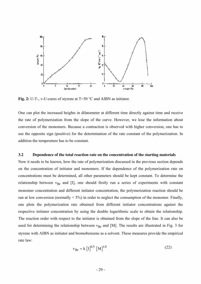
Fig. 2 shows such a time-conversion curve as well as the gross rates as function of the conversion for

the polymerization of styrene, which can be determined by graphical differentiation. This counts

only for bulk reactions (without addition of a solvent). The strange form of the curve is discussed in

5.3.

- 29 -

Fig. 2: U-T-, v-U-cures of styrene at T=50 °C and AIBN as initiator.

One can plot the increased heights in dilatometer at different time directly against time and receive

the rate of polymerization from the slope of the curve. However, we lose the information about

conversion of the monomers. Because a contraction is observed with higher conversion, one has to

use the opposite sign (positive) for the determination of the rate constant of the polymerization. In

addition the temperature has to be constant.

3.2 Dependence of the total reaction rate on the concentration of the starting materials

Now it needs to be known, how the rate of polymerization discussed in the previous section depends

on the concentration of initiator and monomers. If the dependence of the polymerization rate on

concentrations must be determined, all other parameters should be kept constant. To determine the

relationship between vBr and [I], one should firstly run a series of experiments with constant

monomer concentration and different initiator concentration, the polymerization reaction should be

run at low conversion (normally < 5%) in order to neglect the consumption of the monomer. Finally,

one plots the polymerization rate obtained from different initiator concentrations against the

respective initiator concentration by using the double logarithmic scale to obtain the relationship.

The reaction order with respect to the initiator is obtained from the slope of the line. It can also be

used for determining the relationship between vBr and [M]. The results are illustrated in Fig. 3 for

styrene with AIBN as initiator and bromobenzene as a solvent. These measures provide the empirical

rate law:

v k I MBr0.5 1.0 (22)

- 30 -

Fig. 3: Polymerization of styrene with AIBN in brombenzene (T=50°C), a) for [M] = const.; b) for

[I] = const.

4 Other criteria of free-radical polymerization

4.1 Kinetic chain length and degree of polymerization

The kinetic chain length indicates that how many monomer molecules are averagely deposited on

each active polymer radical before the termination takes place. Therefore, is defined as the ratio of

the probability of chain growth Ww to chain termination Wab. Since the probability is proportional to

the corresponding reaction rate, we can write

W

W

v

v

k P * M

k P *

w

ab

w

ab

w

ab2

(23)

Using the definition of the polymerization rate (eq. 15) then follows:

k M

k vw

2 2

ab Br

(24)

The prerequisite for the application of eq. 23 is that the initiator radical and also the growing chains

do not break. At low initiator concentration it can be taken as a good approximation. The degree of

polymerization and the corresponding molecular weights are closely related to the just defined

kinetic chain length. Assuming the validity of the reaction scheme discussed in section 3, the degree

of polymerization in chain termination is defined as follows for the combination:

Pn = 2 .

and for disproportionation:

- 31 -

Pn =

4.2 Chain transfer

One should distinguish between the chain as a term for a linear macromolecule and the chain as

reaction kinetics term; thus, the termination of the growing molecule does not also mean a

termination of the kinetic chain. The chain transfer reaction will occur when a growing chain radical

abstracts an atom from other molecules, for example, hydrogen, chlorine etc., at the same time, the

attacked molecule forms a new radical and initiates a new chain growth. The chain reaction proceeds

continuously, even though the chain growth of the first macromolecule is completed. Chain transfer

reactions can take place with initiator, polymer, monomer, solvent and the polymer radical itself, in

addition, the so-called regulator or chain transfer agent can be added for this purpose. Especially the

last three examples are of practical importance.

When such a chain transfer takes place in the polymerization reaction, an additional reaction should

be added into the reaction scheme, which [P*] is reduced without substantially affecting vBr. XQ is

generally referred to the chain transfer partner whose weakly bound atom X is transferred to the

polymer radical.

vd XQ

dtk P* XQÜ Ü

(25)

In analogy to the kinetic chain length , one defines `for the occurrence of chain transfer:

= v

v + vw

ab Ü

(26)

It includes all the monomers, which are connected by a sequence of chain growth and range from

chain starting or a transfer to the chain termination or a transfer. If no chain transfer takes place, then

´ = . For termination by disproportionation:

P n

For termination by combination it should be considered that two kinds of polymer molecules are

available:

a) Molecules, whose chain growth is terminated by chain transfer:

P n

b) Molecules, whose chain growth is terminated by combination:

P 2 n .

- 32 -

4.3 The Norrish-Trommsdorf-effect (NT-effect, gel-effect)

Following the polymerization to high conversion and assuming the validity of the rate law for

polymerization (eq. 20) we expect that, due to the reduction in monomer concentration, the overall

rate decreases linearly with conversion. The polymerization of styrene in a solvent can very well

explain these phenomena. However, the rate of the polymerization rises disproportionate, if the

polymerization is running in bulk. E. Trommsdorf interpreted this effect as follows:

During the polymerization reaction, the viscosity of the reaction mixture increases to such an extent

as a result of the formation of macromolecules that the mobility of the growing macro-radicals

becomes severely restricted and bimolecular termination is then hindered. However, the reactivity of

the chain ends remains unchanged and simultaneously the formation of the new radical via the

decomposition of initiator and the corresponding polymer radicals carry out continually; furthermore,

the unreacted monomer moves so relatively freely that the propagation reaction occurs continually,

which results in the extension of the kinetic chain. Before reaching 100% conversion, the rate of the

polymerization drops, due to the high viscosity, the monomer is also frozen, and the reaction solution

looks like a gel.

5 Radical copolymerization

By copolymerization we understand the mutual polymerization of two or more chemically different

monomers and the resulting copolymers containing repeat units of all the participating monomers.

The following discussion is limited to the copolymerization of two different monomers.

5.1 Copolymerization equation

In this section the derivation of the copolymerization equation via a kinetic approach is discussed.

For the derivation of the equation, the following assumption must be made:

1. Die polymerization is irreversible, that is to say, there are not reverse reaction in equations

28-31.

2. The total concentrations of monomers [M1] and [M2] are equal to the concentrations at the

reaction site.

3. The degree of polymerization is so high that the consumption of the monomers for

initiation, termination and transferring can be neglected.

4. The influence of the penultimate monomers incorporated in the polymer chain on the

activity of the polymer radicals is negligible.

5. The Bodenstein’ sche quasistationary state should be applied in the kinetic analysis.

- 33 -

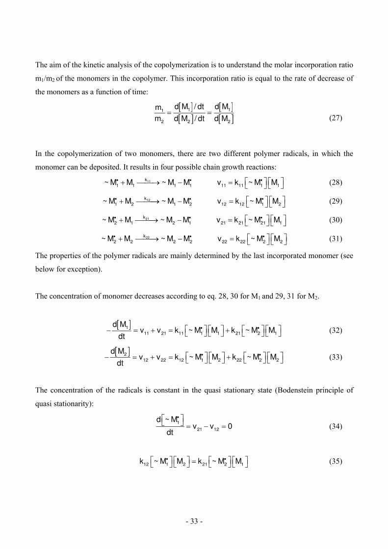
The aim of the kinetic analysis of the copolymerization is to understand the molar incorporation ratio

m1/m2 of the monomers in the copolymer. This incorporation ratio is equal to the rate of decrease of

the monomers as a function of time:

1 11

2 2 2

d M / dt d Mm

m d M / dt d M

(27)

In the copolymerization of two monomers, there are two different polymer radicals, in which the

monomer can be deposited. It results in four possible chain growth reactions:

11k

1 1 1 1 11 11 1 1~ M M ~ M M v k ~ M M (28)

12k

1 2 1 2 12 12 1 2~ M M ~ M M v k ~ M M (29)

21k

2 1 2 1 21 21 21 1~ M M ~ M M v k ~ M M (30)

22k

2 2 2 2 22 22 2 2~ M M ~ M M v k ~ M M (31)

The properties of the polymer radicals are mainly determined by the last incorporated monomer (see

below for exception).

The concentration of monomer decreases according to eq. 28, 30 for M1 and 29, 31 for M2.

1

11 21 11 1 1 21 2 1

d Mv v k ~ M M k ~ M M

dt

(32)

2

12 22 12 1 2 22 2 2

d Mv v k ~ M M k ~ M M

dt

(33)

The concentration of the radicals is constant in the quasi stationary state (Bodenstein principle of

quasi stationarity):

1

21 12

d ~ Mv v 0

dt

(34)

12 1 2 21 2 1k ~ M M k ~ M M (35)

- 34 -

By using eq. 35, the concentration of the active species [~M2●] can be expressed via [~M1

●]. The

copolymerization equation (37) can be obtained by introduction of eq. 32, 33 and 35 into eq. 27,

concomitantly, r1, r2 are defined as copolymerization parameter.

11 221 2

12 21

k kr und r

k k (36)

1 1 1 21

2 2 2 2 1

M r M Mm

m M r M M

(37)

5.2 Influence of the penultimate incorporated monomers (penultimate effect)

If the penultimate incorporated monomer influences the reactivity of the growing chain end, the two

rate constants should be different:

111

211

k

1 1 1 1 1 1

k

2 1 1 2 1 1

~ M M M ~ M M M

~ M M M ~ M M M

That is to say, eight different propagation constants have to be considered for copolymerization of

two monomers. An impact is observed, when the last but one monomer has a strong inductive effect

on the added monomer (e.g., in the fumaronitrile/styrene system).

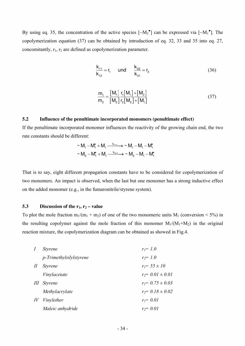
5.3 Discussion of the r1, r2 – value

To plot the mole fraction m1/(m1 + m2) of one of the two monomeric units M1 (conversion < 5%) in

the resulting copolymer against the mole fraction of this monomer M1/(M1+M2) in the original

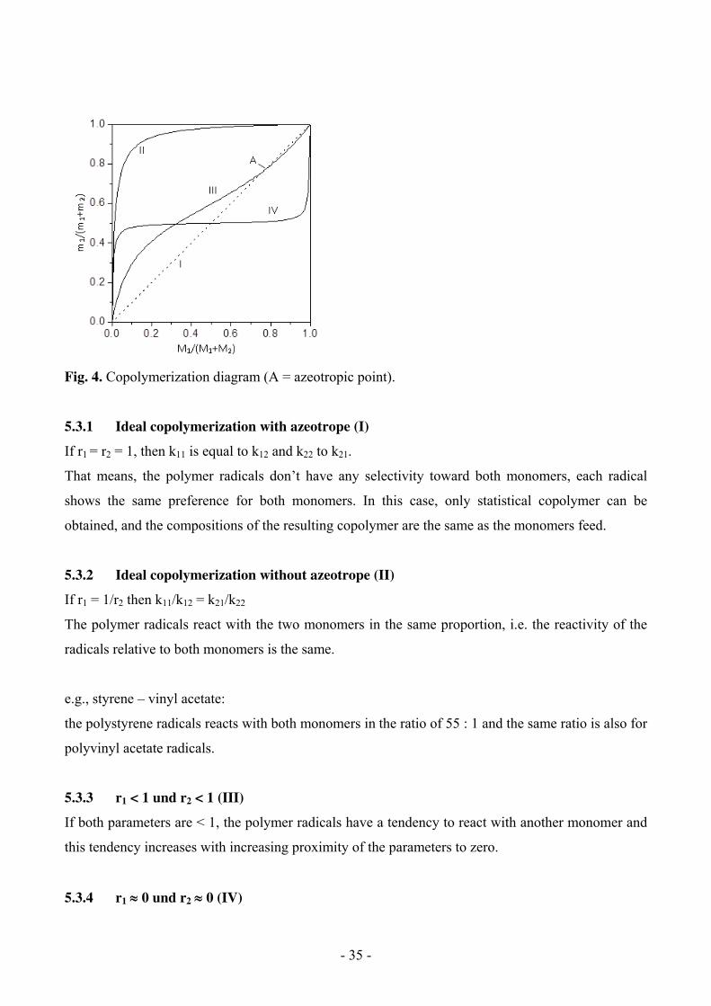
reaction mixture, the copolymerization diagram can be obtained as showed in Fig.4.

I Styrene r1= 1.0

p-Trimethylsilylstyrene r2= 1.0

II Styrene r1= 55 ± 10

Vinylacetate r2= 0.01 ± 0.01

III Styrene r1= 0.75 ± 0.03

Methylacrylate r2= 0.18 ± 0.02

IV Vinylether r1= 0.01

Maleic anhydride r2= 0.01

- 35 -

Fig. 4. Copolymerization diagram (A = azeotropic point).

5.3.1 Ideal copolymerization with azeotrope (I)

If r1 = r2 = 1, then k11 is equal to k12 and k22 to k21.

That means, the polymer radicals don’t have any selectivity toward both monomers, each radical

shows the same preference for both monomers. In this case, only statistical copolymer can be

obtained, and the compositions of the resulting copolymer are the same as the monomers feed.

5.3.2 Ideal copolymerization without azeotrope (II)

If r1 = 1/r2 then k11/k12 = k21/k22

The polymer radicals react with the two monomers in the same proportion, i.e. the reactivity of the

radicals relative to both monomers is the same.

e.g., styrene – vinyl acetate:

the polystyrene radicals reacts with both monomers in the ratio of 55 : 1 and the same ratio is also for

polyvinyl acetate radicals.

5.3.3 r1 < 1 und r2 < 1 (III)

If both parameters are < 1, the polymer radicals have a tendency to react with another monomer and

this tendency increases with increasing proximity of the parameters to zero.

5.3.4 r1 0 und r2 0 (IV)

- 36 -

Here the growing polymer radicals react only with the other monomer. This results in a polymer

chain, in which both monomers will be polymerized alternatively (alternating copolymer). The

polymerization usually ends if one of the monomer is completely used.

5.3.5 r1 > 1 and r2 > 1

The larger the parameter, the more easily the polymer radical reacts with its own monomers. For

very large r1 and r2 block copolymerization or simultaneous homopolymerization of both monomers

takes place. In the last case (though observed very rarely) a polymer blend is formed.

5.4 Experimental determination of the copolymerization parameters

For determining the copolymerization parameters r1 and r2, a monomer mixture of known

composition is polymerized at low conversion (<5%) in order to assume [M1] = [M1]0 and [M2] =

[M2]0. The composition of the obtained copolymer can then be determined by using analytical

methods, e.g., elemental analysis, UV-, NMR-, IR- spectroscopy, radiolabelled monomers or GC

analysis of the residual monomers. In principle, it is possible to calculate both r1 and r2 from the

composition of only two copolymers that have been obtained from two different mixtures of both

monomers. However, due to the uncertainty of the analytical methods, it is recommended to

determine the composition of the copolymers from several monomer mixtures and evaluate the

results by graphical methods.

5.4.1 Graphical determination of the copolymerization parameters according to Mayo and

Lewis

The linear relationship between r1 and r2 is obtained from the rearranged copolymerization equation

37:

2

2 21 11 2 2

2 1 21

M Mm mr r 1

m M mM

(38)

Slope and intercept of this equation are known, each copolymerization can then be characterized via

a linear relationship of r1 = f (r2) (Fig. 5). In practice, the lines for all copolymerization do not

intersect precisely at a point so that r1 and r2 are taken as the center of the smallest area that is cut or

touched by all the lines, the size of this area allows an estimate of the limits of error.

- 37 -

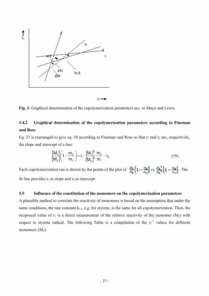
Fig. 5. Graphical determination of the copolymerization parameters acc. to Mayo and Lewis.

5.4.2 Graphical determination of the copolymerization parameters according to Fineman

und Ross

Eq. 37 is rearranged to give eq. 39 according to Fineman und Ross so that r1 and r2 are, respectively,

the slope and intercept of a line:

2

1

2

2

2

2

11

1

2

2

1 rm

m

M

Mr

m

m1

M

M

(39)

Each copolymerization run is shown by the points of the plot of vs. . The

fit line provides r1 as slope and r2 as intercept.

5.5 Influence of the constitution of the monomers on the copolymerization parameters

A plausible method to correlate the reactivity of monomers is based on the assumption that under the

same conditions, the rate constant k11, e.g. for styrene, is the same for all copolymerization. Then, the

reciprocal value of r1 is a direct measurement of the relative reactivity of the monomer (M2) with

respect to styrene radical. The following Table is a compilation of the r1-1 values for different

monomers (M2):

- 38 -

Table 1: Relative reactivity (r1-1) of radicals (~ M1

●) against the monomer (M2).

2M 1~ M

styrene butadiene AN MMA

2-vinylpyridin 1.82 - 8.84 2.50

2-chlorostyrene 1.79 0.85 - 2.00

4-vinylpyridin 1.61 - 8.84 1.74

4-chlorstyrol 1.35 0.69 - 2.41

styrene 1.00 0.61 25.0 2.18

α-methylstyrene 0.85 - 16.7 2.00

The following effects are taken into account for the realization of the results:

5.5.1 Resonance stabilization of monomers and polymer radicals

The overall rate of polymerization for the homopolymerization depends on the resonance

stabilization of both in the monomer and the polymer. As shown in Table 2, the stabilization ability

of radical formed after the addition of a monomer has a huge influence on the total rate of

polymerization.

Table 2: Addition rate of a polymer radical to its own monomer and the resonance of the radical and

monomers.

Monomer relative rate of

addition

Resonance stabilization energy [kcal/mol]

double bond radical

vinyl acetate 23.0 1.7 4

MMA 7.05 4.2 23

styrene 1.45 4.2 24.5

butadiene 1 6.0 25

A decrease in resonance stabilization energy results in an increase of the reactivity of the radical. A

stable radical is not reactive enough for the reaction with a double bond (which would result in the

formation of a less stable radical). For copolymerization this means that only compounds with

similar radical stabilities can react with each other. The polystyrene radical (~M1*) is not reactive

- 39 -

enough to react with vinylacetate (M2) because this would form a less stable radical. So preferebly

another styrene monomer would react with the polystyrene radical.

5.5.2 Influence of the double bond polarity on the copolymerization parameters

The polarity of a double bond has a minor influence on the total rate of the homopolymerization

compared to the radical stability. However, the polarity of double bond plays a very important role in

the copolymerization, especially, on little stabilized radical types. Taken styrene as example, one can

see that the rate of addition of monomer M2 increases (i.e. r1 becomes smaller) if there are strong

electron-accepting substituents on M2. This tendency becomes predominant in case both monomers

yield similar resonance-stabilized radicals. Here, one should also assume that the polarity of the

obtained radical is the same as that of the monomer. If the polarity of the monomers is different

enough, they can copolymerize themselves, i.e. vinyl ether with styrene or maleic anhydride. There

are two possible interpretations for this behavior:

1. At the time of addition of monomers to the growing polymer radical, the monomer will

orient in such a way that the activation energy of the addition steps become very low, if

radical and monomers are oppositely polarized.

2. The monomers are pre-oriented like a charge-transfer complex (confirmed by charge-

transfer band in the UV). By partial charge transfer, the complex will obtain a “diradical”

character. This kind of polymerization reaction can, therefore, be thought of as

polycombination reaction (i.e. vinyl ether – maleic anhydride).

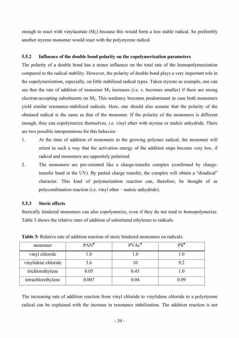
5.5.3 Steric effects

Sterically hindered monomers can also copolymerize, even if they do not tend to homopolymerize.

Table 3 shows the relative rates of addition of substituted ethylenes to radicals.

Table 3: Relative rate of addition reaction of steric hindered monomers on radicals.

monomer PAN● PVAc● PS●

vinyl chloride 1.0 1.0 1.0

vinylidene chloride 3.6 10 9.2

trichlorethylene 0.05 0.45 1.0

tetrachlorethylene 0.007 0.04 0.09

The increasing rate of addition reaction from vinyl chloride to vinylidene chloride to a polystyrene

radical can be explained with the increase in resonance stabilization. The addition reaction is not

- 40 -

hindered sterically with both monomers, but the increasing steric hindrance from trichloroethylene to

tetrachloroethylene causes a decrease of the relative reaction rate, although the stability of the radical

increases. (Fig. 6).

Fig. 6: Steric hindrance of the addition reaction for a 1,2-substituted ethylene.

5.5.4 Influences of the solvent, temperature and phase relationship on copolymerization

An influence of the solvent on the copolymerization of two monomers is to be expected when a

monomer associated or the solubility of both monomers is different in heterogeneous polymerization.

The processes of association on the polymer become particularly noticeable when the polymerization

is heterogeneous and the association of both monomers is obviously different. In addition, the

association of the polymers is strongly temperature dependent. For the styrene/MMA system, there is

no association effect, so the parameters approach the value 1 at a high temperature, which means, the

selectivity of the polymer radical decreases towards the monomers.

6 Statistics of the copolymer

Due to the nature of the formation process, the length and composition of the obtained polymer chain

follow different distribution functions, the measured properties on a copolymer sample are only an

average value and do not represent the structure of a single polymer chain. Of course, it is impossible

to detect the sequence of any length and any structure by analytical means using currently available

methods. With the help of nuclear magnetic resonance, the sequence of up to 5 repeating units can

now be identified quantitatively.

6.1 Sequence distribution in copolymers

The appearing frequency of sequences with one, two, three, etc. constitutional units of the same

monomer is determined by the probability of the addition of the monomer in question in the

copolymer chain. The probability p12 for the formation of M1-M2-sequence is defined by the ratio of

the rate of addition to the sum of all possible rate of addition, as shown in eq. 40:

12 1 212

12

11 12 11 1 2 12 1 2

k M Mvp

v v k M M k M M

(40)

- 41 -

Eq. 41 is obtained if eq. 40 is divided by k12 [M1*][M2] via elimination of the unknown concentration

M1● .

12

1

1

2

1p

M1 r

M

(41)

According to the above-mentioned rule, the probability of p21 and p22 can be formulated.

Furthermore, equation 42 should be fulfilled:

p11 + p12 + p22 = 1 (42)

By calculating the probability from the r-parameter and the initial concentration of the monomers,

the relationship between the formal kinetic of the copolymerization and the statistic structure of the

copolymer chain is made.

6.2 Calculation of the average sequence length ( I1)

The frequency of any sequence length from M1 and/or M2-unit can be calculated by using the above-

mentioned probability.

The average sequence length for monomer M1 is obtained as follows:

111

12

v1

v l (43)

or can be written as eq. 44 if the rate of reaction is substituted by eq. 28-31:

11 1 1 11 1

1

12 1 1 12 1

k M M k M1 1

k M M k M

l (44)

taken

111

12

kr

k (45)

then the average sequence length 1l of monomers M1 is expressed as:

1

1 1

2

Mr 1

M

l (46)

and similarly for the average sequence length 2l

2

2 2

1

Mr 1

M

l (47)

- 42 -

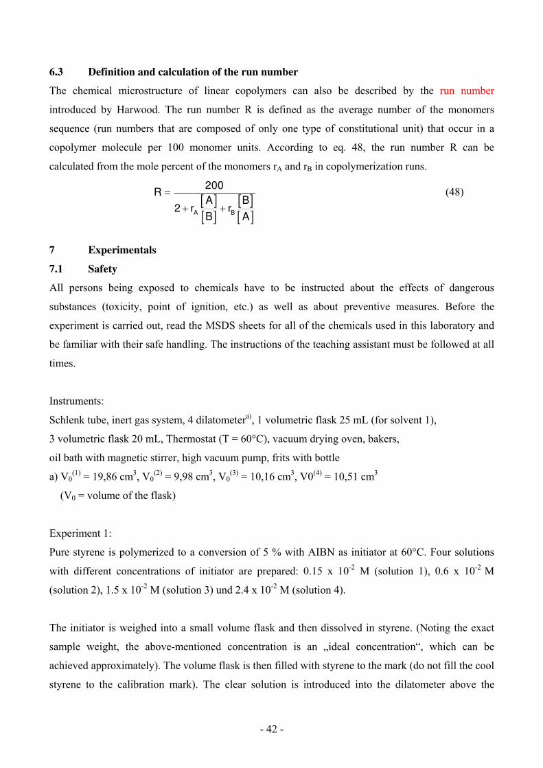
6.3 Definition and calculation of the run number

The chemical microstructure of linear copolymers can also be described by the run number

introduced by Harwood. The run number R is defined as the average number of the monomers

sequence (run numbers that are composed of only one type of constitutional unit) that occur in a

copolymer molecule per 100 monomer units. According to eq. 48, the run number R can be

calculated from the mole percent of the monomers rA and rB in copolymerization runs.

A B

200R

A B2 r r

B A

(48)

7 Experimentals

7.1 Safety

All persons being exposed to chemicals have to be instructed about the effects of dangerous

substances (toxicity, point of ignition, etc.) as well as about preventive measures. Before the

experiment is carried out, read the MSDS sheets for all of the chemicals used in this laboratory and

be familiar with their safe handling. The instructions of the teaching assistant must be followed at all

times.

Instruments:

Schlenk tube, inert gas system, 4 dilatometera), 1 volumetric flask 25 mL (for solvent 1),

3 volumetric flask 20 mL, Thermostat (T = 60°C), vacuum drying oven, bakers,

oil bath with magnetic stirrer, high vacuum pump, frits with bottle

a) V0(1) = 19,86 cm3, V0

(2) = 9,98 cm3, V0(3) = 10,16 cm3, V0(4) = 10,51 cm3

(V0 = volume of the flask)

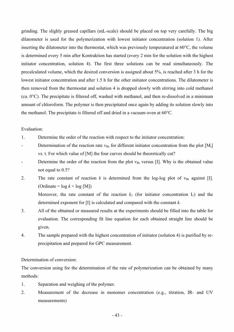
Experiment 1:

Pure styrene is polymerized to a conversion of 5 % with AIBN as initiator at 60°C. Four solutions

with different concentrations of initiator are prepared: 0.15 x 10-2 M (solution 1), 0.6 x 10-2 M

(solution 2), 1.5 x 10-2 M (solution 3) und 2.4 x 10-2 M (solution 4).

The initiator is weighed into a small volume flask and then dissolved in styrene. (Noting the exact

sample weight, the above-mentioned concentration is an „ideal concentration“, which can be

achieved approximately). The volume flask is then filled with styrene to the mark (do not fill the cool

styrene to the calibration mark). The clear solution is introduced into the dilatometer above the

- 43 -

grinding. The slighly greased capillars (mL-scale) should be placed on top very carefully. The big

dilatometer is used for the polymerization with lowest initiator concentration (solution 1). After

inserting the dilatometer into the thermostat, which was previously temperatured at 60°C, the volume

is determined every 5 min after Kontraktion has started (every 2 min for the solution with the highest

initiator concentration, solution 4). The first three solutions can be read simultaneously. The

precalculated volume, which the desired conversion is assigned about 5%, is reached after 3 h for the

lowest initiator concentration and after 1.5 h for the other initiator concentrations. The dilatometer is

then removed from the thermostat and solution 4 is dropped slowly with stirring into cold methanol

(ca. 0°C). The precipitate is filtered off, washed with methanol, and then re-dissolved in a minimum

amount of chloroform. The polymer is then precipitated once again by adding its solution slowly into

the methanol. The precipitate is filtered off and dried in a vacuum oven at 60°C.

Evaluation:

1. Determine the order of the reaction with respect to the initiator concentration:

- Determination of the reaction rate vBr for different initiator concentration from the plot [Mt]

vs. t. For which value of [M] the four curves should be theoretically cut?

- Determine the order of the reaction from the plot vBr versus [I]. Why is the obtained value

not equal to 0.5?

2. The rate constant of reaction k is determined from the log-log plot of vBr against [I].

(Ordinate = log k + log [M])

Moreover, the rate constant of the reaction k1 (for initiator concentration I1) and the

determined exponent for [I] is calculated and compared with the constant k.

3. All of the obtained or measured results at the experiments should be filled into the table for

evaluation. The corresponding fit line equation for each obtained straight line should be

given.

4. The sample prepared with the highest concentration of initiator (solution 4) is purified by re-

precipitation and prepared for GPC measurement.

Determination of conversion:

The conversion using for the determination of the rate of polymerization can be obtained by many

methods:

1. Separation and weighing of the polymer.

2. Measurement of the decrease in monomer concentration (e.g., titration, IR- and UV

measurements)

- 44 -

3. Measurement of the refractive index

4. Measurement of the volume contract (dilatometer)

The most straighforward method for the determination of conversion is to observe the volume

contraction, which is based on the difference in density between the monomer and the polymer. The

volume contraction is for a 100% conversion at 25 °C, for example, 14.1 % for styrene, 26.8% for

vinyl acetate, 23.1 % for methyl methacrylate and 25.0% for isoprene. From experience, it can be

linearly interpolated for low conversion. In addition to the high sensitivity (conversion < 1%), the

application of the dilatometric method depends in particular on the fact that the density of a polymer

does not depend on the degree of polymerization and minor structural difference. The respective

monomer concentration [M]t can be calculated from the partial density of the monomer M and

polymer P in solution:

MV V

V

10

M

mol

ltt

t

3

M-1

P-1

M

(49)

MM= 104.14 g mol-1 M= 0.924 - 9.17 x 10-4 T

Vt= volume at t P= 1.087 - 7.00 x 10-4 T

V0= volume at t = 0 T= temperature in °C

V = m V 0

P

0 M

P

Experiment 2:

Monomers are weighed into the Schlenk flask according to the below-given mixing ratio and then

0.5 mol-% AIBN are added.

Table 4: Mixing ratio of both monomers.

styrene [mL] MMA [mL]

bottle 1 2 10

bottle 2 4 8

bottle 3 6 6

bottle 4 8 4

bottle 5 10 2

- 45 -

Important: the accurate information of the mixing rate (weighing!).

For degassing, the Schlenk flask is connected to the vacuum line, frozen by using liquid nitrogen,

evacuated, and then thawed with the tap closed. The flask is filled with nitrogen and then frozen

again. The process as described above is repeated twice. (Attention: vacuum grease disturbs the

spectroscopic investigation!)

The thawing can be considerably accelerated by immersing the flask in methanol and three flasks can

be degassed at the same time. The flask is then warmed to room temperature, removed from the inert

gas system under nitrogen, and then sealed with a glass stopper. The flask is put into an oil bath,

which is kept at 50 °C by using a thermostat. (note the time!). After one hour of polymerization

(corresponding to an approximate turnover of 5-10%), the flask is then removed from the oil bath

and the polymer is precipitated by adding the solution dropwise to 150 – 200 mL of methanol, the

precipitate is filtered off, washed carefully with methanol and dried in a vacuum oven at 40°C.

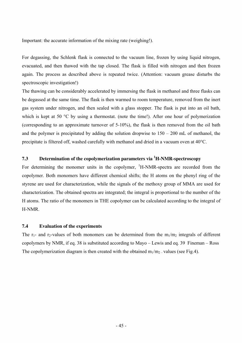
7.3 Determination of the copolymerization parameters via 1H-NMR-spectroscopy

For determining the monomer units in the copolymer, 1H-NMR-spectra are recorded from the

copolymer. Both monomers have different chemical shifts; the H atoms on the phenyl ring of the

styrene are used for characterization, while the signals of the methoxy group of MMA are used for

characterization. The obtained spectra are integrated; the integral is proportional to the number of the

H atoms. The ratio of the monomers in THE copolymer can be calculated according to the integral of

H-NMR.

7.4 Evaluation of the experiments

The r1- and r2-values of both monomers can be determined from the m1/m2 integrals of different

copolymers by NMR, if eq. 38 is substituted according to Mayo – Lewis and eq. 39 Fineman – Ross

The copolymerization diagram is then created with the obtained m1/m2 – values (see Fig.4).

- 46 -

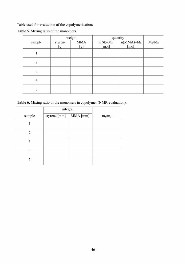
Table used for evaluation of the copolymerization:

Table 5. Mixing ratio of the monomers.

weight quantity sample styrene

[g] MMA

[g] n(St)=M1

[mol] n(MMA)=M2

[mol] M1/M2

1

2

3

4

5

Table 6. Mixing ratio of the monomers in copolymer (NMR-evaluation).

integral

sample styrene [mm] MMA [mm] m1/m2

1

2

3

4

5

- 47 -

8 Questions:

1. Discuss the presence of oxygen in the radical polymerization. Is it possible to use it as an

initiator?

2. Explain the term ceiling-temperature? Does a floor-temperature exist too?

3. Under which conditions is the relation vw [I]0.5 false?

4. Draw the diagrams for vBr against conversion and P against conversion (in solution). How

do the same diagrams for polycondensation and ionic polymerization look like? ( P against

conversion)

5. How does the termination rate change in the case of the NT-effect?

6. The activation energy of the decomposition of AIBN is ca. 30 kcal/mol. For the activation

energy the gross rate of the polymerization of styrene is ca. 20 kcal/mol. How does the gross

rate and the degree of polymerization change at low conversions if you decrease the

temperature from 40 to 20 °C (neglect side reactions)?

7. What is a block copolymer and graft copolymer and how would you synthesize them?

8. What is an „ideal“ copolymerization and how does the copolymerization diagram look like?

9. What consequences would you expect for the structure of a copolymer for the following r-

parameters:

r1 = 1.00 r2 > 1.00

r1 = 1.00 r2 < 1.00

r1 0 r2 0

r1 r2 .

10. What composition of a copolymer is expected for r1 0 and r2 0?

11. List methods for the experimental determination of the composition of copolymers?

12. Which values for r1 and r2 are needed for the formation of an azeotrope?

13. Are there structural differences between polymers made by radical or anionic

copolymerizations (at which r1 and r2)?

14. What extremes in the sequence distribution are possible in copolymers?

15. List requirements for a statistical derivation of the copolymerization equation?

16. How does the copolymerization diagram for r1 > 1 and r2 > 1 look like?

17. What is an alternating copolymerization?

18. Why do you observe several signals in the 1H-NMR spectrum for the methoxy group in a

copolymer (only 1 signal in the PMMA monomer spectrum)?

- 48 -

19. Determine the average sequence length and the number of blocks for the monomers styrene

and vinylidenechloride (r1=2.0, r2=0.14). Monomer concentrations are 30 mol% styrene and

70 mol% vinylidenechloride. Explain.

- 49 -

Rheology

1 Introduction .............................................................................................................................. 50

2 Theoretical foundation ................................................................................................................ 50

2.1 Fundamental terms in rheology............................................................................................ 50

2.2 Linear-viscoelastic behavior ............................................................................................... 52

2.3 Measuring technique ......................................................................................................... 55

2.3.1 Oscillation measurements ...................................................................................... 55

2.3.2 Rotational experiments .......................................................................................... 56

2.3.3 Tension experiment .............................................................................................. 57

2.3.4 Relaxation experiment ........................................................................................... 57

2.4 Borderline behavior of matter and rheological models .............................................................. 57

2.4.1 Elastic behavior ................................................................................................... 58

2.4.2 Plastic behavior .................................................................................................... 59

2.4.3 Viscous behavior .................................................................................................. 60

2.4.4 Viscoelastic behavior ............................................................................................ 61

2.4.5 Characterization by flow and viscosity curves ............................................................ 63

2.5 Time-dependent rheological behavior ................................................................................... 64

2.6 Rheometry (measuring technique) ........................................................................................ 65

3 Experimental ............................................................................................................................ 66

3.1 Conduction of rotational measurements ................................................................................. 66

3.2 Time-dependent change of viscosity ..................................................................................... 67

3.3 Oscillation measurements to determine the viscoelastic behavior ............................................... 67

4 Questions ................................................................................................................................. 68

5 Literature ................................................................................................................................. 68

- 50 -

1 Introduction

Rheology is the science which describes, explains, quantifies and applies the phenomena appearing

while bodies or liquids are deformed or while they flow. According to Ziabicki [1], the rheological

behavior is responsible for the drawability and thus of fundamental importance for the spinnability of

liquid systems. Further examples of applied rheology are found in various areas in natural science

and engineering. [2-7]

1. Colors and varnish (brushability, storage)

2. Polymer solutions and melts (polymer extrusion and spinning

3. Characterization of polymers (statement about molecular weights and molecular weight

distribution

4. Manufacture of high performance materials (ceramics)

5. Flow behavior of food (ketchup, convenience sauce)

6. Cosmetics and sanitary products (tooth paste, cream, shampoos)

7. Geo-rheology (simulation of volcanic flow)

8. Medicine (hemorheology)

9. Pharmaceutical products

10. Electronics

In the following paragraphs the basic principles of rheology, which are described in literature [1 –

20] are addressed.

2 Theory

2.1 Fundamental terms in rheology

To characterize the flow behavior of substances, they are subjected to defined forces and the

resulting deformations are described in detail in dependence of different parameters. Depending on

the direction of the affecting force, the relevant cases for rheometry are distinguished: elongation,

compression strain and shear strain. The effect occurring during the shear experiment of a liquid and

the associated fundamental terms in rheology can be explained with the aid of a two-plate-model

(Figure 1). In this model a liquid is located between two parallel plates of the area A. The upper plate

is moved relative to the lower static plate with a constant velocity. Thereby the power F needs to be

applied due to the internal friction. This shear strain causes a laminar flow of the velocity v which

linearly decreases from the moving to the static plate.

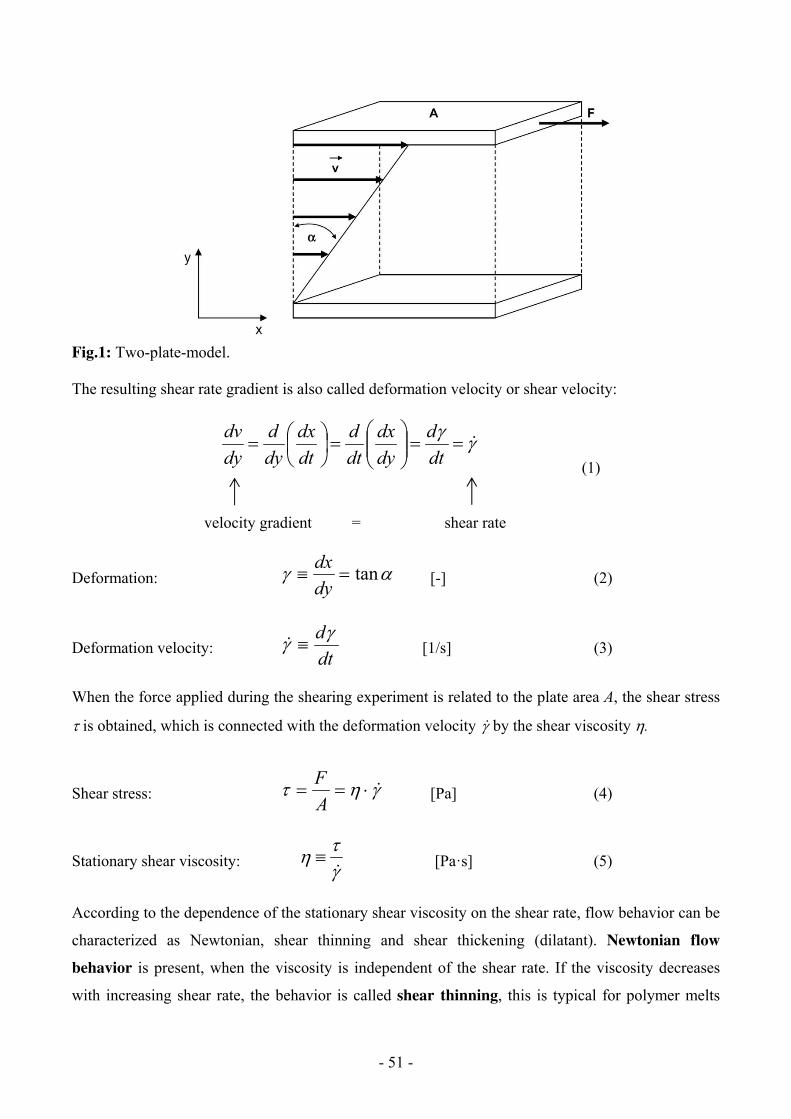
- 51 -

Fig.1: Two-plate-model. The resulting shear rate gradient is also called deformation velocity or shear velocity:

dt

d

dy

dx

dt

d

dt

dx

dy

d

dy

dv

(1)

velocity gradient = shear rate

Deformation: tandy

dx [-] (2)

Deformation velocity: dt

d [1/s] (3)

When the force applied during the shearing experiment is related to the plate area A, the shear stress

is obtained, which is connected with the deformation velocity by the shear viscosity .

Shear stress: A

F [Pa] (4)

Stationary shear viscosity:

[Pa·s] (5)

According to the dependence of the stationary shear viscosity on the shear rate, flow behavior can be

characterized as Newtonian, shear thinning and shear thickening (dilatant). Newtonian flow

behavior is present, when the viscosity is independent of the shear rate. If the viscosity decreases

with increasing shear rate, the behavior is called shear thinning, this is typical for polymer melts

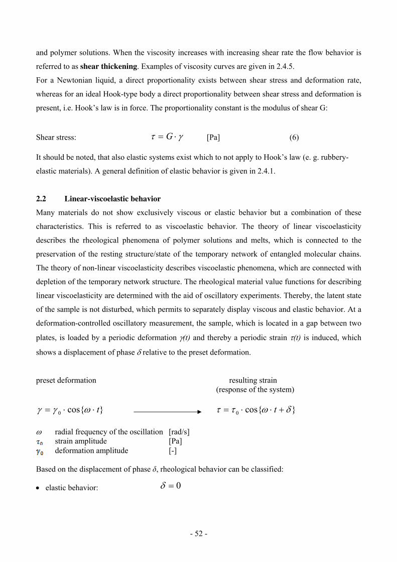
- 52 -

and polymer solutions. When the viscosity increases with increasing shear rate the flow behavior is

referred to as shear thickening. Examples of viscosity curves are given in 2.4.5.

For a Newtonian liquid, a direct proportionality exists between shear stress and deformation rate,

whereas for an ideal Hook-type body a direct proportionality between shear stress and deformation is

present, i.e. Hook’s law is in force. The proportionality constant is the modulus of shear G:

Shear stress: G [Pa] (6)

It should be noted, that also elastic systems exist which to not apply to Hook’s law (e. g. rubbery-

elastic materials). A general definition of elastic behavior is given in 2.4.1.

2.2 Linear-viscoelastic behavior

Many materials do not show exclusively viscous or elastic behavior but a combination of these

characteristics. This is referred to as viscoelastic behavior. The theory of linear viscoelasticity

describes the rheological phenomena of polymer solutions and melts, which is connected to the

preservation of the resting structure/state of the temporary network of entangled molecular chains.

The theory of non-linear viscoelasticity describes viscoelastic phenomena, which are connected with

depletion of the temporary network structure. The rheological material value functions for describing

linear viscoelasticity are determined with the aid of oscillatory experiments. Thereby, the latent state

of the sample is not disturbed, which permits to separately display viscous and elastic behavior. At a

deformation-controlled oscillatory measurement, the sample, which is located in a gap between two

plates, is loaded by a periodic deformation (t) and thereby a periodic strain (t) is induced, which

shows a displacement of phase relative to the preset deformation.

preset deformation resulting strain (response of the system)

}cos{0 t }cos{0 t

radial frequency of the oscillation [rad/s]

strain amplitude [Pa] deformation amplitude [-]

Based on the displacement of phase δ, rheological behavior can be classified:

elastic behavior: 0

- 53 -

viscous behavior: 2

viscoelastic behavior: 2

0

Fig. 2: Course of strain and deformation during oscillatory measurements.

To simplify rheological calculations, complex values are introduced. The transition to complex

values is performed by extending strain and deformation with the respective imaginary part. This

allows the transition from trigonometric functions to the complex e-function, thus simplifying

calculations considerably. The following rheological values are defined:

Complex shear strain:

)}(exp{})sin{}(cos{* 00 titit (7)

Complex deformation:

}exp{})sin{}(cos{* 00 titit (8)

Complex deformation velocity:

}exp{*)(* 0 tiidt

d

(9) Viscoelastic behavior can be described by the complex modulus G*, which is defined as the quotient

of complex strain and complex deformation.

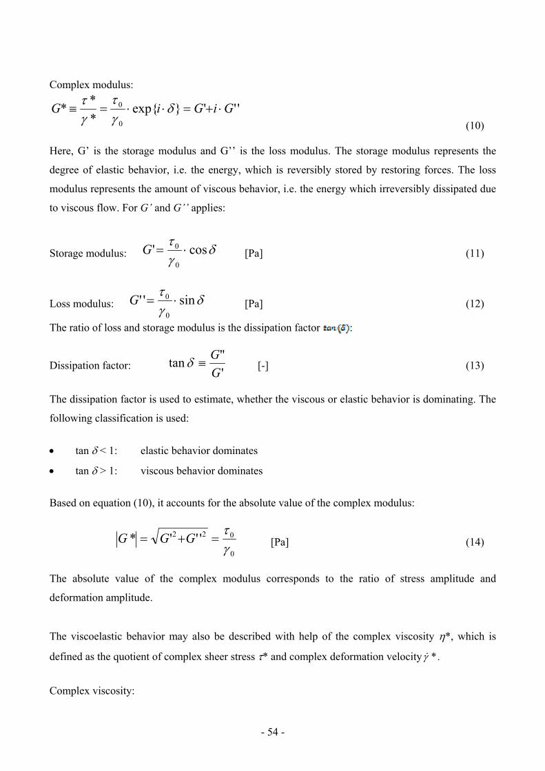
- 54 -

Complex modulus:

'''}exp{*

**

0

0 GiGiG

(10)

Here, G’ is the storage modulus and G’’ is the loss modulus. The storage modulus represents the

degree of elastic behavior, i.e. the energy, which is reversibly stored by restoring forces. The loss

modulus represents the amount of viscous behavior, i.e. the energy which irreversibly dissipated due

to viscous flow. For G’ and G’’ applies:

Storage modulus:

cos'0

0 G [Pa] (11)

Loss modulus:

sin''0

0 G [Pa] (12)

The ratio of loss and storage modulus is the dissipation factor :

Dissipation factor: '

"tan

G

G [-] (13)

The dissipation factor is used to estimate, whether the viscous or elastic behavior is dominating. The

following classification is used:

tan < 1: elastic behavior dominates

tan > 1: viscous behavior dominates

Based on equation (10), it accounts for the absolute value of the complex modulus:

0

022 '''*

GGG [Pa] (14)

The absolute value of the complex modulus corresponds to the ratio of stress amplitude and

deformation amplitude.

The viscoelastic behavior may also be described with help of the complex viscosity *, which is

defined as the quotient of complex sheer stress * and complex deformation velocity * .

Complex viscosity:

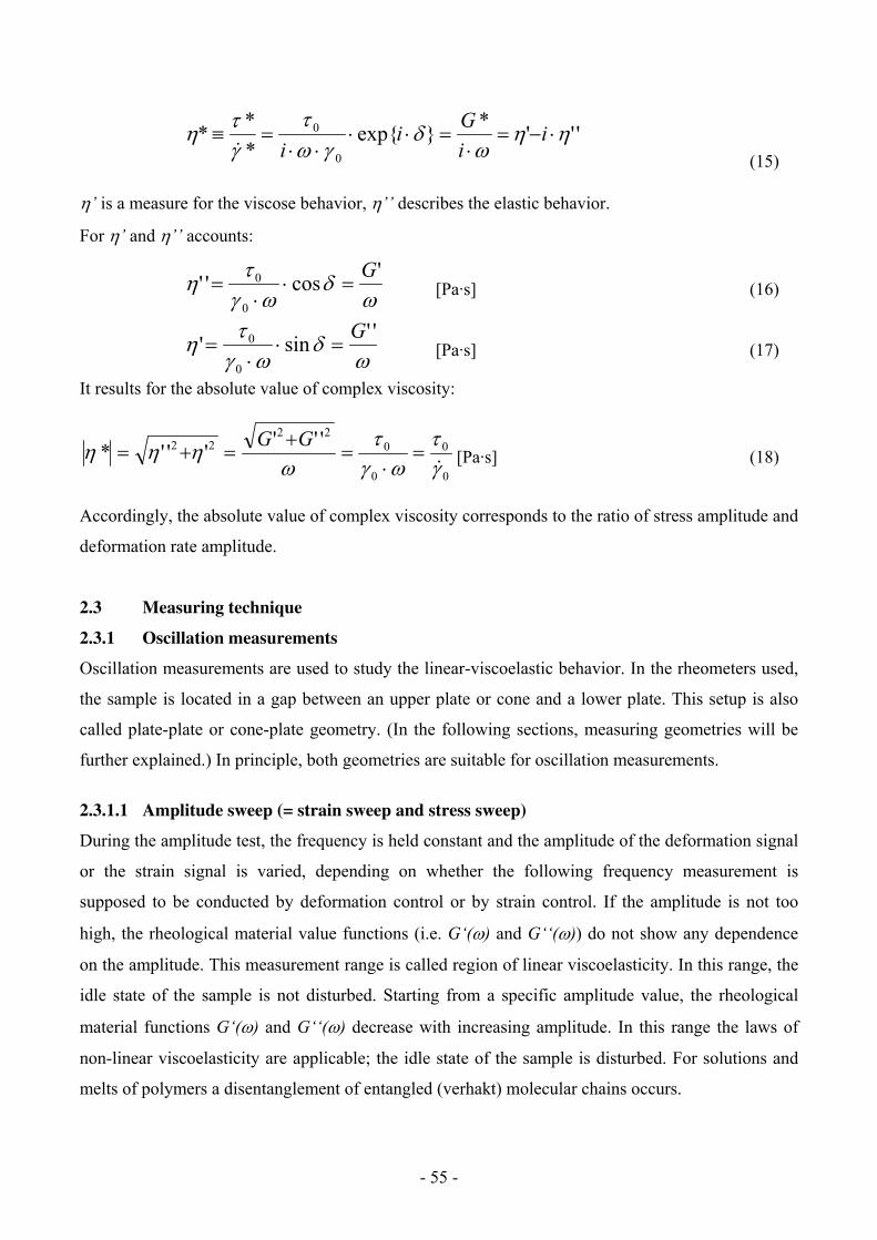
- 55 -

'''*

}exp{*

**

0

0

i

i

Gi

i (15)

’ is a measure for the viscose behavior, ’’ describes the elastic behavior.

For ’ and ’’ accounts:

'

cos''0

0 G

[Pa·s] (16)

''

sin'0

0 G

[Pa·s] (17)

It results for the absolute value of complex viscosity:

0

0

0

022

22 ''''''*

GG [Pa·s] (18)

Accordingly, the absolute value of complex viscosity corresponds to the ratio of stress amplitude and

deformation rate amplitude.

2.3 Measuring technique

2.3.1 Oscillation measurements

Oscillation measurements are used to study the linear-viscoelastic behavior. In the rheometers used,

the sample is located in a gap between an upper plate or cone and a lower plate. This setup is also

called plate-plate or cone-plate geometry. (In the following sections, measuring geometries will be

further explained.) In principle, both geometries are suitable for oscillation measurements.

2.3.1.1 Amplitude sweep (= strain sweep and stress sweep)

During the amplitude test, the frequency is held constant and the amplitude of the deformation signal

or the strain signal is varied, depending on whether the following frequency measurement is

supposed to be conducted by deformation control or by strain control. If the amplitude is not too

high, the rheological material value functions (i.e. G‘() and G‘‘()) do not show any dependence

on the amplitude. This measurement range is called region of linear viscoelasticity. In this range, the

idle state of the sample is not disturbed. Starting from a specific amplitude value, the rheological

material functions G‘() and G‘‘() decrease with increasing amplitude. In this range the laws of

non-linear viscoelasticity are applicable; the idle state of the sample is disturbed. For solutions and

melts of polymers a disentanglement of entangled (verhakt) molecular chains occurs.

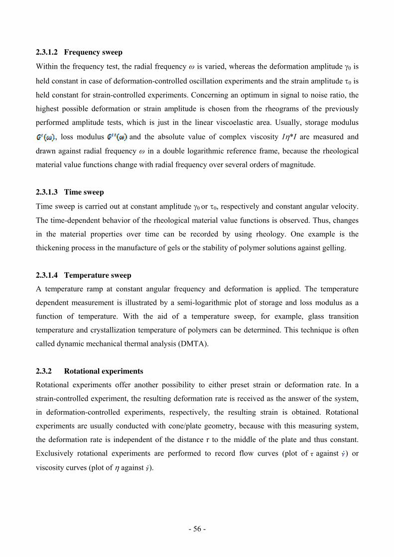
- 56 -

2.3.1.2 Frequency sweep

Within the frequency test, the radial frequency ω is varied, whereas the deformation amplitude 0 is

held constant in case of deformation-controlled oscillation experiments and the strain amplitude 0 is

held constant for strain-controlled experiments. Concerning an optimum in signal to noise ratio, the

highest possible deformation or strain amplitude is chosen from the rheograms of the previously

performed amplitude tests, which is just in the linear viscoelastic area. Usually, storage modulus

, loss modulus and the absolute value of complex viscosity I*I are measured and

drawn against radial frequency ω in a double logarithmic reference frame, because the rheological

material value functions change with radial frequency over several orders of magnitude.

2.3.1.3 Time sweep

Time sweep is carried out at constant amplitude 0 or 0, respectively and constant angular velocity.

The time-dependent behavior of the rheological material value functions is observed. Thus, changes

in the material properties over time can be recorded by using rheology. One example is the

thickening process in the manufacture of gels or the stability of polymer solutions against gelling.

2.3.1.4 Temperature sweep

A temperature ramp at constant angular frequency and deformation is applied. The temperature

dependent measurement is illustrated by a semi-logarithmic plot of storage and loss modulus as a

function of temperature. With the aid of a temperature sweep, for example, glass transition

temperature and crystallization temperature of polymers can be determined. This technique is often

called dynamic mechanical thermal analysis (DMTA).

2.3.2 Rotational experiments

Rotational experiments offer another possibility to either preset strain or deformation rate. In a

strain-controlled experiment, the resulting deformation rate is received as the answer of the system,

in deformation-controlled experiments, respectively, the resulting strain is obtained. Rotational

experiments are usually conducted with cone/plate geometry, because with this measuring system,

the deformation rate is independent of the distance r to the middle of the plate and thus constant.

Exclusively rotational experiments are performed to record flow curves (plot of against ) or

viscosity curves (plot of against ).

- 57 -

2.3.3 Tension experiment

This experiment is a rotational experiment in which the time-dependent behavior of rheological

quantities is recorded. Here, a constant deformation rate is preset and the resulting strain signal is

measured as a function of time. In the ideal case of the experiment, the angular frequency escalates

from the idle state to a constant value. Viscoelastic liquids exhibit a delayed increase in shear stress.

If the measured time-dependent shear stress is correlated to the preset constant deformation rate, the

time-dependent (transient) viscosity +(t) is obtained:

)()(

tt

[Pa·s] (19)

In the case of viscoelastic fluids the transient viscosity approximates a boundary value with

progressing measurement time. This boundary value is called stationary (= time-independent) shear

viscosity :

)(),(lim

tt

[Pa·s] (20)

2.3.4 Relaxation experiment

In the relaxation experiment, the sample is stressed by an escalating deformation o and the resulting

strain signal (t), which decreases with time, is measured. Due to its elastic restoring force a strain is

produced by the preset deformation. A relaxation process within the sample takes place by viscous

flow and the generated strain diminishes. If the strain signal is correlated with the preset

deformation, the nonlinear-viscoelastic relaxation modulus is obtained, with is dependent of time and

the existent deformation:

Relaxation modulus: 0

0

)(),(

t

tG [Pa]

(t): strain [Pa] o: deformation [-]

2.4 Borderline behavior of matter and rheological models

In rheometry material-specific dependencies of the above mentioned interactions of applied shear

stress and resulting shear deformation are obtained. Thereby, the material’s behavior is distinguished

by the following properties: viscous, elastic, viscoelastic and plastic behavior. These behaviors of

material are sketched in Figure 3. All liquids can be described with the aid of viscosity.

- 58 -

Fig. 3: Boundary behavior of matter: (1) elastic (steel), (2) plastic (modelling clay), (3) viscous (water), (4) viscoelastic (silicone rubber).

2.4.1 Elastic behavior

Upon application of strain, which is held constant over a certain period of time, an elastic material

experiences a deformation, which is constant over time, too (Figure 4). In case a strain is applied as a

step function, the resulting deformation shows the same escalating behavior. Solids with this

behavior are defined elastic. If there is an additional directly proportional ratio between applied

strain and the resulting deformation, the solid is called Hookean solids, i.e. Hook’s law is applicable

(see section 2.1, eq. 6). Note that also elastic solids exist, that do not follow Hook’s law, i.e. strain

and deformation are not linearly connected to each other (e. g., materials for which the law of rubber-

elasticity is applicable).

Fig. 4: Definition of elasticity in general: applied strain as a step function and resulting deformation

of escalating behavior.

t t0 t1

t t1

responseinput

(1) (2) (3) (4)

t0

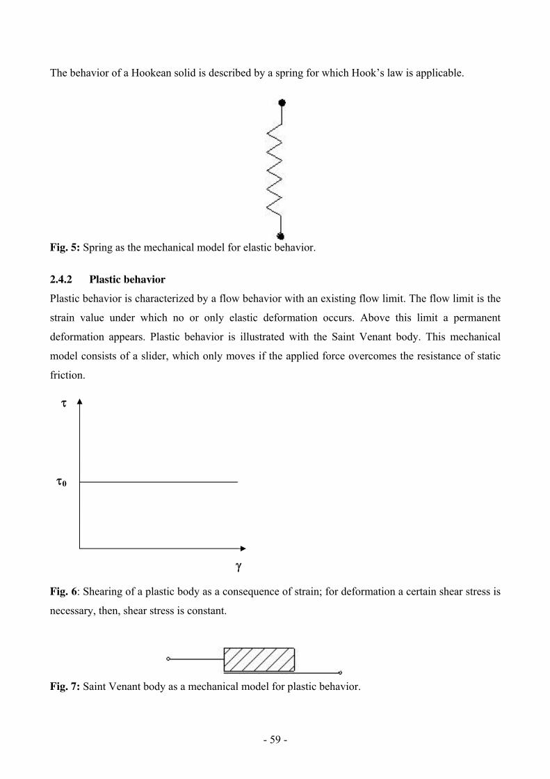
- 59 -

The behavior of a Hookean solid is described by a spring for which Hook’s law is applicable.

Fig. 5: Spring as the mechanical model for elastic behavior.

2.4.2 Plastic behavior

Plastic behavior is characterized by a flow behavior with an existing flow limit. The flow limit is the

strain value under which no or only elastic deformation occurs. Above this limit a permanent

deformation appears. Plastic behavior is illustrated with the Saint Venant body. This mechanical

model consists of a slider, which only moves if the applied force overcomes the resistance of static

friction.

Fig. 6: Shearing of a plastic body as a consequence of strain; for deformation a certain shear stress is

necessary, then, shear stress is constant.

Fig. 7: Saint Venant body as a mechanical model for plastic behavior.

0

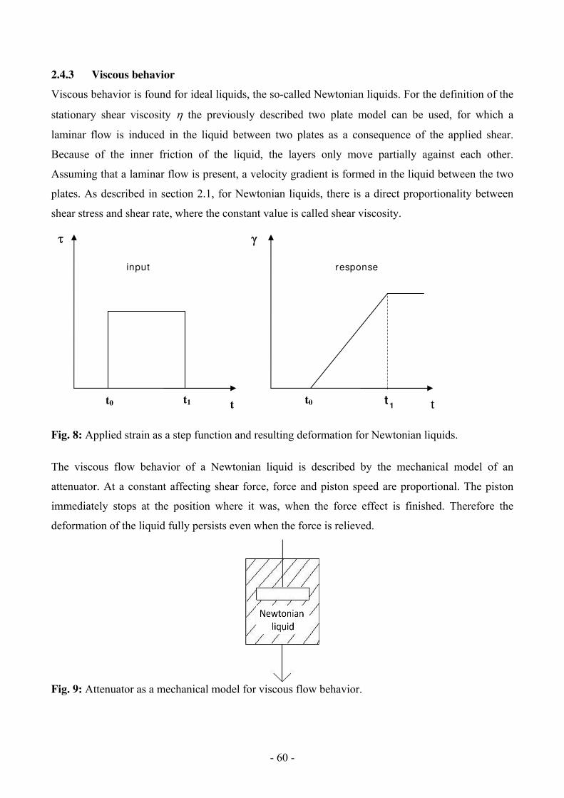
- 60 -

2.4.3 Viscous behavior

Viscous behavior is found for ideal liquids, the so-called Newtonian liquids. For the definition of the

stationary shear viscosity the previously described two plate model can be used, for which a

laminar flow is induced in the liquid between two plates as a consequence of the applied shear.

Because of the inner friction of the liquid, the layers only move partially against each other.

Assuming that a laminar flow is present, a velocity gradient is formed in the liquid between the two

plates. As described in section 2.1, for Newtonian liquids, there is a direct proportionality between

shear stress and shear rate, where the constant value is called shear viscosity.

Fig. 8: Applied strain as a step function and resulting deformation for Newtonian liquids.

The viscous flow behavior of a Newtonian liquid is described by the mechanical model of an

attenuator. At a constant affecting shear force, force and piston speed are proportional. The piston

immediately stops at the position where it was, when the force effect is finished. Therefore the

deformation of the liquid fully persists even when the force is relieved.

Fig. 9: Attenuator as a mechanical model for viscous flow behavior.

t t0 t1

t t1

response

t0

input

- 61 -

2.4.4 Viscoelastic behavior

As described in section 2.2 many materials do not show exclusively viscous or elastic behavior, but a

combination of both properties. Depending on the type of strain that is applied to the material, the

respective components of viscoelastic flow behavior appear more or less pronounced. Rheological

material value functions used for describing viscoelastic flow behavior are given in section 2.2.

Viscoelastic behavior can be described by mechanical models where spring and attenuator are

combined. For describing the behavior of viscoelastic liquids (polymer melts or concentrated

polymer solutions) one or several Maxwell elements are used. A Maxwell element is a series of

connected springs and attenuators. If a force is applied in form of a step function, the result is a

spontaneous deflection (elastic behavior). Then, the effect of the attenuator appears (viscous

behavior). The initial position is not reached again. This model describes the ideal behavior of

viscoelastic liquids.

Fig. 10: Applied strain as a step function and resulting deformation for a simple Maxwell element.

Fig. 11: Maxwell element as a simple mechanical model for viscoelastic liquids.

For many viscoelastic liquids this model does not describe the flow behavior adequately enough.

Only by parallel connection of several Maxwell elements viscoelastic liquids can be described with

satisfactory accuracy. This approach is called generalized Maxwell model.

t t0 t1

t t1 t

0

spring

at tenuator

regression of

the spring

input response

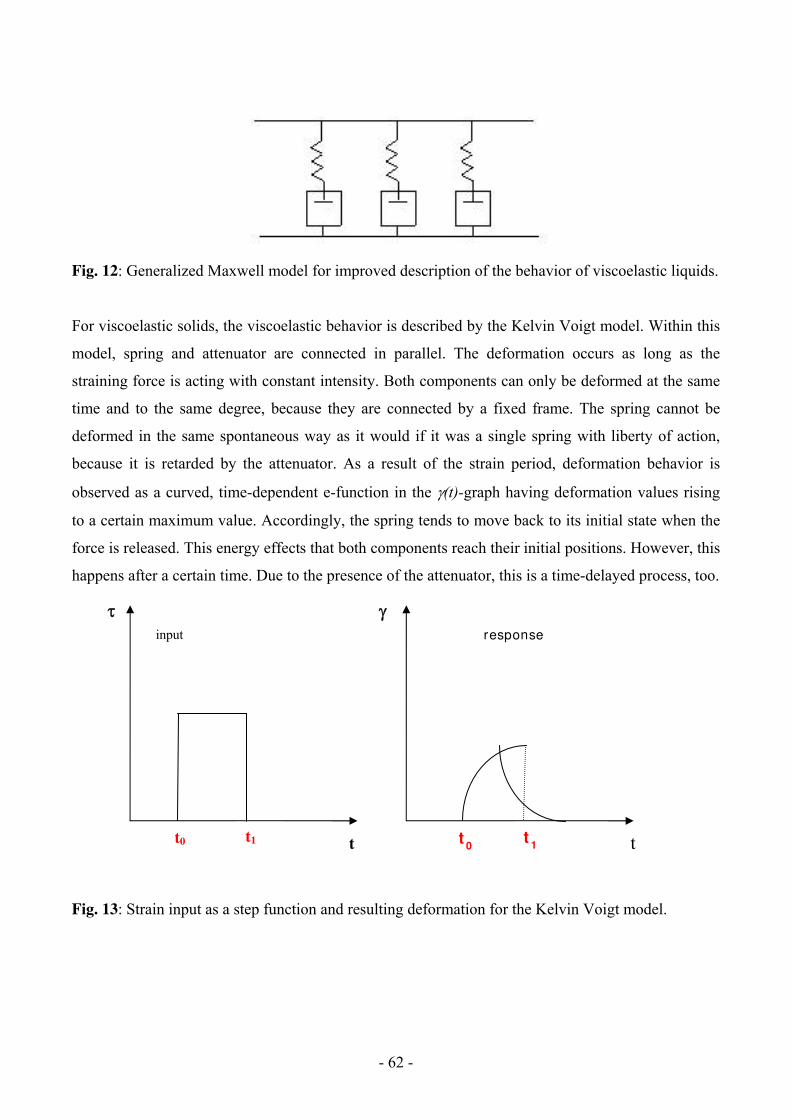
- 62 -

Fig. 12: Generalized Maxwell model for improved description of the behavior of viscoelastic liquids.

For viscoelastic solids, the viscoelastic behavior is described by the Kelvin Voigt model. Within this

model, spring and attenuator are connected in parallel. The deformation occurs as long as the

straining force is acting with constant intensity. Both components can only be deformed at the same

time and to the same degree, because they are connected by a fixed frame. The spring cannot be

deformed in the same spontaneous way as it would if it was a single spring with liberty of action,

because it is retarded by the attenuator. As a result of the strain period, deformation behavior is

observed as a curved, time-dependent e-function in the (t)-graph having deformation values rising

to a certain maximum value. Accordingly, the spring tends to move back to its initial state when the

force is released. This energy effects that both components reach their initial positions. However, this

happens after a certain time. Due to the presence of the attenuator, this is a time-delayed process, too.

Fig. 13: Strain input as a step function and resulting deformation for the Kelvin Voigt model.

t t0 t1

t t1 t

0

responseinput

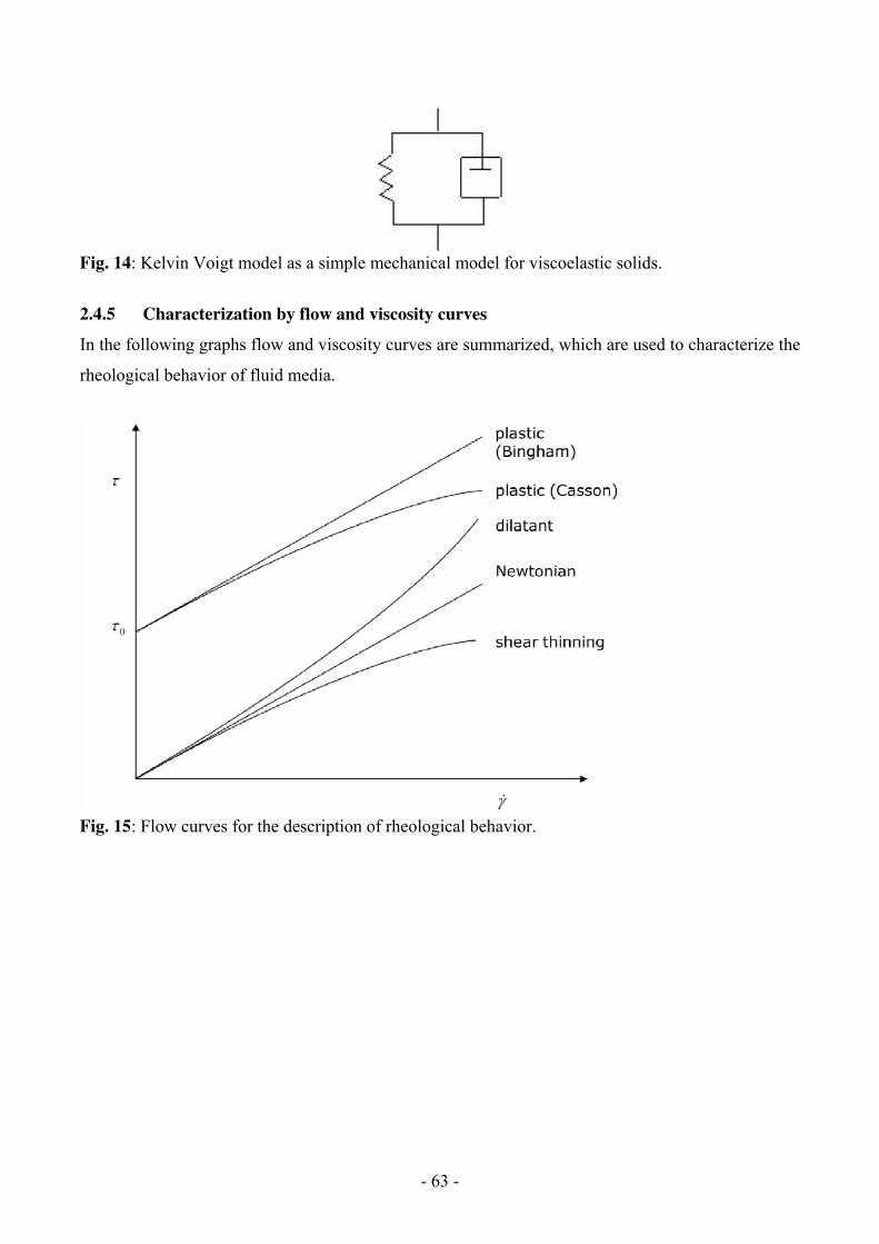
- 63 -

Fig. 14: Kelvin Voigt model as a simple mechanical model for viscoelastic solids.

2.4.5 Characterization by flow and viscosity curves

In the following graphs flow and viscosity curves are summarized, which are used to characterize the

rheological behavior of fluid media.

Fig. 15: Flow curves for the description of rheological behavior.

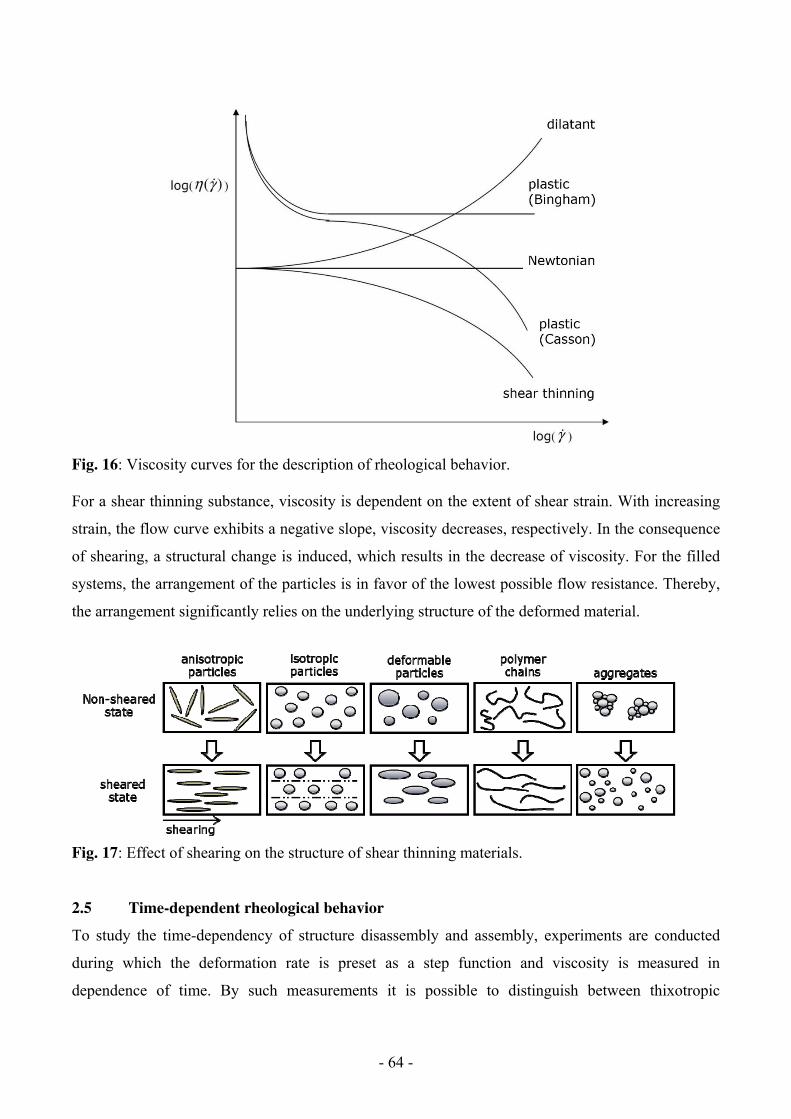
- 64 -

Fig. 16: Viscosity curves for the description of rheological behavior. For a shear thinning substance, viscosity is dependent on the extent of shear strain. With increasing

strain, the flow curve exhibits a negative slope, viscosity decreases, respectively. In the consequence

of shearing, a structural change is induced, which results in the decrease of viscosity. For the filled

systems, the arrangement of the particles is in favor of the lowest possible flow resistance. Thereby,

the arrangement significantly relies on the underlying structure of the deformed material.

Fig. 17: Effect of shearing on the structure of shear thinning materials.

2.5 Time-dependent rheological behavior

To study the time-dependency of structure disassembly and assembly, experiments are conducted

during which the deformation rate is preset as a step function and viscosity is measured in

dependence of time. By such measurements it is possible to distinguish between thixotropic

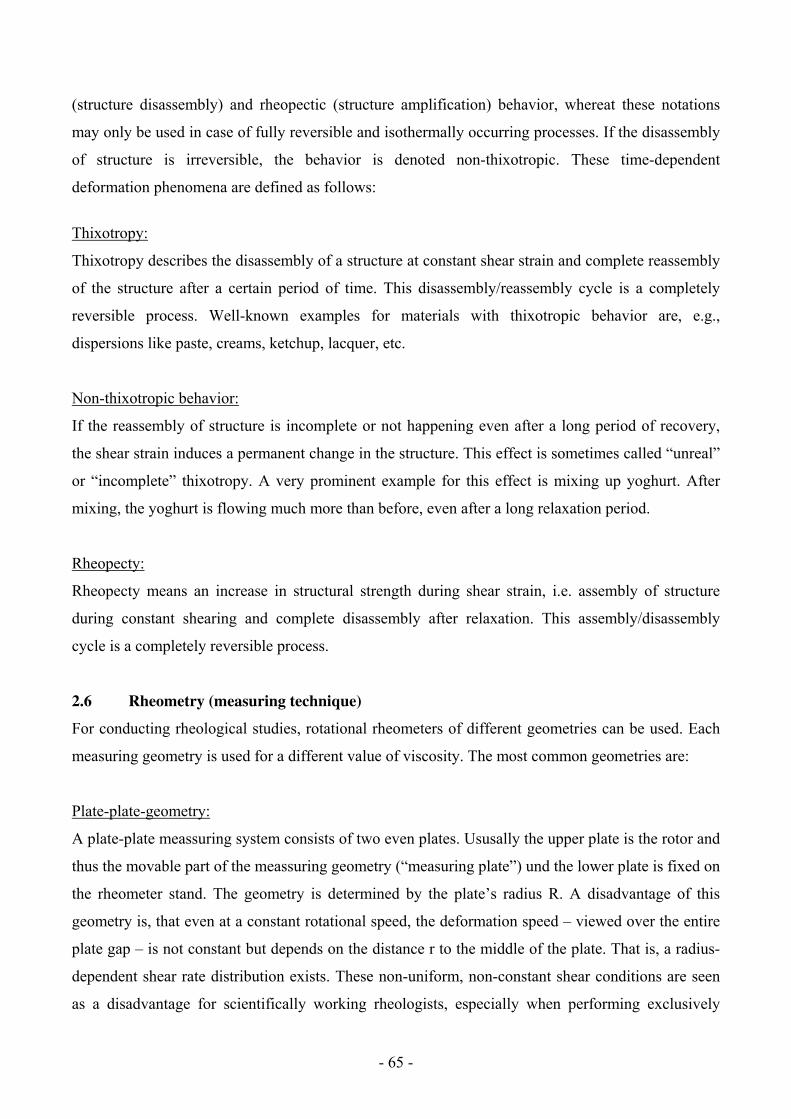
- 65 -

(structure disassembly) and rheopectic (structure amplification) behavior, whereat these notations

may only be used in case of fully reversible and isothermally occurring processes. If the disassembly

of structure is irreversible, the behavior is denoted non-thixotropic. These time-dependent

deformation phenomena are defined as follows:

Thixotropy:

Thixotropy describes the disassembly of a structure at constant shear strain and complete reassembly

of the structure after a certain period of time. This disassembly/reassembly cycle is a completely

reversible process. Well-known examples for materials with thixotropic behavior are, e.g.,

dispersions like paste, creams, ketchup, lacquer, etc.

Non-thixotropic behavior:

If the reassembly of structure is incomplete or not happening even after a long period of recovery,

the shear strain induces a permanent change in the structure. This effect is sometimes called “unreal”

or “incomplete” thixotropy. A very prominent example for this effect is mixing up yoghurt. After

mixing, the yoghurt is flowing much more than before, even after a long relaxation period.

Rheopecty:

Rheopecty means an increase in structural strength during shear strain, i.e. assembly of structure

during constant shearing and complete disassembly after relaxation. This assembly/disassembly

cycle is a completely reversible process.

2.6 Rheometry (measuring technique)

For conducting rheological studies, rotational rheometers of different geometries can be used. Each

measuring geometry is used for a different value of viscosity. The most common geometries are:

Plate-plate-geometry:

A plate-plate meassuring system consists of two even plates. Ususally the upper plate is the rotor and

thus the movable part of the meassuring geometry (“measuring plate”) und the lower plate is fixed on

the rheometer stand. The geometry is determined by the plate’s radius R. A disadvantage of this

geometry is, that even at a constant rotational speed, the deformation speed – viewed over the entire

plate gap – is not constant but depends on the distance r to the middle of the plate. That is, a radius-

dependent shear rate distribution exists. These non-uniform, non-constant shear conditions are seen

as a disadvantage for scientifically working rheologists, especially when performing exclusively

- 66 -

rotational experiments. These experiments should be conducted with cone-plate geometry for the

above mentioned reasons. However, this disadvantage is of low relevance when determining

rheological material value constants of linear viscoelasticity (that is G’, G’’ and I*I), for this reason,

the plate-plate geometry is often used for performing oscillation measurements, especially when the

sample is analyzed at different temperatures or, if the sample is filled with particles (e. g., filled

polymer melts or dispersions with relatively large particles). Plate-plate geometry allows for larger

gap positions, thus, phenomena which negatively affect the measured values, like thermal expansion

of the measuring tools or friction effects due to incorporated particles in filled systems could be

minimized.

Cone-plate geometry:

A cone-plate measuring system consists of a round measurement body with a slightly tilted, slightly

cone-shaped surface and a plate. Usually, the cone is the rotor and hence, the upper, moveable part of

the measuring geometry and the lower plate is unmovably fixed on the rheometer stand. The

dimensions of the conical surface are determined by the cone’s radius R and the cone angle α. A

major advantage of the cone-plate geometry is that with this measurement system, the deformation

rate is independent of the distance r to the middle of the plate. Because of this relationship, cone-

plate geometry is especially recommended for performing rotational experiments.

Coaxial cylinder geometry:

Coaxial cylinder measuring systems consist of a measurement body (inner cylinder) and a measuring

cup (outer cylinder). Coaxial means that both cylindrical components are located along one identical

rotationally symmetric axis when the system is in working position. These measuring systems are

especially used for studying low viscous liquids. According to the operating mode, two system types

are distinguished. In the Couette system, the outer cylinder is rotating whereas in the Searle system,

it is the inner cylinder.

3 Experimental

All experiments are conducted with a cone-system (Ø=50 mm, cone-plate-geometry). Temperature

control of the plate is conducted by a Peltier element. Unless stated otherwise, all experiments are

carried out at a temperature of T = 25 °C.

3.1 Conduction of rotational measurements

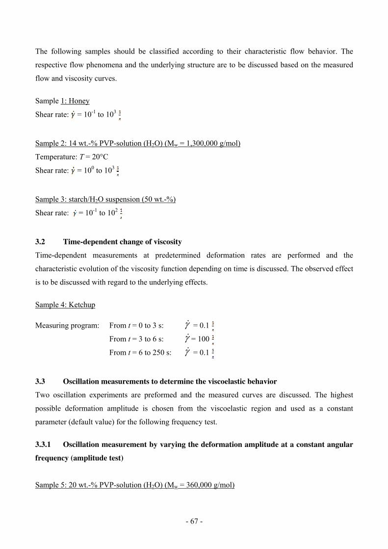
- 67 -

The following samples should be classified according to their characteristic flow behavior. The

respective flow phenomena and the underlying structure are to be discussed based on the measured

flow and viscosity curves.

Sample 1: Honey

Shear rate: = 10-1 to 103

Sample 2: 14 wt.-% PVP-solution (H2O) (Mw = 1,300,000 g/mol)

Temperature: T = 20°C

Shear rate: = 100 to 103

Sample 3: starch/H2O suspension (50 wt.-%)

Shear rate: = 10-1 to 102

3.2 Time-dependent change of viscosity

Time-dependent measurements at predetermined deformation rates are performed and the

characteristic evolution of the viscosity function depending on time is discussed. The observed effect

is to be discussed with regard to the underlying effects.

Sample 4: Ketchup

Measuring program: From t = 0 to 3 s: = 0.1

From t = 3 to 6 s: = 100

From t = 6 to 250 s: = 0.1

3.3 Oscillation measurements to determine the viscoelastic behavior

Two oscillation experiments are preformed and the measured curves are discussed. The highest

possible deformation amplitude is chosen from the viscoelastic region and used as a constant

parameter (default value) for the following frequency test.

3.3.1 Oscillation measurement by varying the deformation amplitude at a constant angular

frequency (amplitude test)

Sample 5: 20 wt.-% PVP-solution (H2O) (Mw = 360,000 g/mol)

- 68 -


Measuring program: angular frequency: ω = 10 rad/s

Deformation amplitude from = 1 % to 1000 %

Illustration of G’, G’’ and as a function of the deformation amplitude and choice of the

deformation amplitude from the measured curves for the subsequent oscillation measurement (from

linear viscoelastic to non-linear viscoelastic behavior).

3.3.2 Oscillation measurement by varying the angular frequency


Measuring program: Use of the deformation amplitude determined in 3.3.1 as a default

Angular frequency from ω = 100 to 0.1 rad/s

Illustration of G’, G’’ and as a function of angular frequency. Explain the rheological behavior

based on the depicted curves (viscosity, viscoelasticity and elasticity). Describe the structural events

at the transition between the borderline cases.

4 Questions

1. Term other applied examples for the determination of materials’ viscosity.

2. Sketch the most important flow and viscosity diagrams.

3. Describe the advantages and disadvantages of plate/plate and cone/plate geometry.

5 Literature

1. M. Dragoni, A. Tallarico, J. Volcanol. Geoth. Res. (1994), 59, 241

2. G. Miyamoto, S. Sasaki, Computers & Geosciences (1996), 23, 283

3. G. B. Thurston, Biophys. J. (1972), 12, 1205

4. W.P. Cox, E.H. Merz: J. Polym. Sci. (1958), 28, 619

5. G. Böhme, M. Stenger: Chem. Eng. Technol. (1988), 11, 199

6. G. V. Vinogradov, A. Y. Malkin, Y. G. Yanovsky, E. A. Dzyura V. F. Schumsky, V. G.

Kulichikhin: Rheol. Acta 8 (1969), 490-496

7. G. V. Vinogradov, N. V. Prozorovskaya: Rheol. Acta 3 (1964)

8. G. V. Vinogradov, A. Y. Malkin: J. Polym. Sci. A: Polym. Chem. (1964), 2, 2357

9. H. M. Laun: Progr. Coll. Pol. Sci. (1987), 75, 111

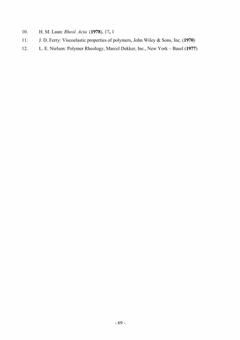
- 69 -

10. H. M. Laun: Rheol. Acta (1978), 17, 1

11. J. D. Ferry: Viscoelastic properties of polymers, John Wiley & Sons, Inc. (1970)

12. L. E. Nielsen: Polymer Rheology, Marcel Dekker, Inc., New York – Basel (1977)

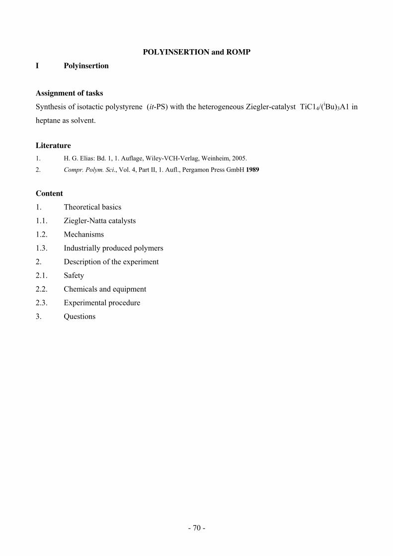
- 70 -

POLYINSERTION and ROMP

I Polyinsertion

Assignment of tasks

Synthesis of isotactic polystyrene (it-PS) with the heterogeneous Ziegler-catalyst TiC14/(iBu)3A1 in

heptane as solvent.

Literature

1. H. G. Elias: Bd. 1, 1. Auflage, Wiley-VCH-Verlag, Weinheim, 2005.

2. Compr. Polym. Sci., Vol. 4, Part II, 1. Aufl., Pergamon Press GmbH 1989

Content

1. Theoretical basics

1.1. Ziegler-Natta catalysts

1.2. Mechanisms

1.3. Industrially produced polymers

2. Description of the experiment

2.1. Safety

2.2. Chemicals and equipment

2.3. Experimental procedure

3. Questions

- 71 -

1 Theoretical basics

1.1 Ziegler-Natta catalysts

In the last few years, transition metal-based catalysts have gained great importance, especially for the

polymerization of ethylene at low pressures, as well as for the synthesis of polypropylene.

Furthermore, they offer a wide range of applications in the preparation of stereoregular polymers.

Among the technically most important catalysts in this area are the so-called Ziegler-catalysts (also

named Ziegler-Natta-catalysts). Systems, which are made by mixing organometallic compounds of

transition group elements IV-VIII with metals alkyls or metals hydrides of the groups I – III of the

periodic system, are referred as Ziegler-catalyst. A typical Ziegler-catalyst is formed, for example,

by the reaction of TiCl4 with Et3Al. These catalysts is heterogeneous, because they precipitate as a

fine suspension in an organic solvent (for example from heptane). At the beginning of catalyst

research, this heterogeneity was assumed to be responsible for catalyst activity (“catalytic surfaces”),

however, Kaminsky et al. found that also soluble (homogeneous) systems display similar activities.

Such homogeneous Ziegler-catalysts can be generated through the combination of, e.g.,

bis(cyclopentadienyl)titanium(IV) dichloride (Cp2TiCl2, a metallocene catalyst) with

diethylaluminiumchloride (Et2AlCl).

A few further important catalytic systems:

Et2AlCl/TiCl3 heterogeneous

Et2AlCl/VCl4/anisole homogeneous

Et2AlCl/V(acac)3 homogeneous

Et2AlCl/Cr(acac)3 homogeneous

Cp2ZrMe2/alumoxane homogeneous

Besides the Ziegler-catalyst, the so-called "Phillips-catalyst" (CrO3/SiO2/A12O3) is of technical

importance, especially in the polymerization of ethylene.

1.2 Mechanisms

The polymerization occurs at the transition metal-carbon bond. The active species and the reaction

mechanism are, with the exception of Phillips-catalysts, mostly clarified. The growth step can

principally take place over a mono- or bimetallic mechanism.

- 72 -

Monometallic mechanism

In the so-called monometallic mechanism (Fig. 1) it is assumed that the olefin approaches first to a

vacant site of the transition metal with its π-bond, and then coordinates to it. The coordinated

monomer is then inserted into the metal-carbon bond via a four-membered transition state.

Fig. 1: Monometallic mechanism.

The main group metal complex is not involved into the chain growth reaction; it is only used for the

alkylation of the transition metal complex ("monometallic"). There are (idealized) separated ion

pairs. In fact, however, these ion pairs are in reality never completely separated from each other, and

the termination and transfer reactions can be easily explained via the following reaction scheme:

Termination caused by β-hydride elimination:

Transfer to the monomer:

Molecular weight control by H2:

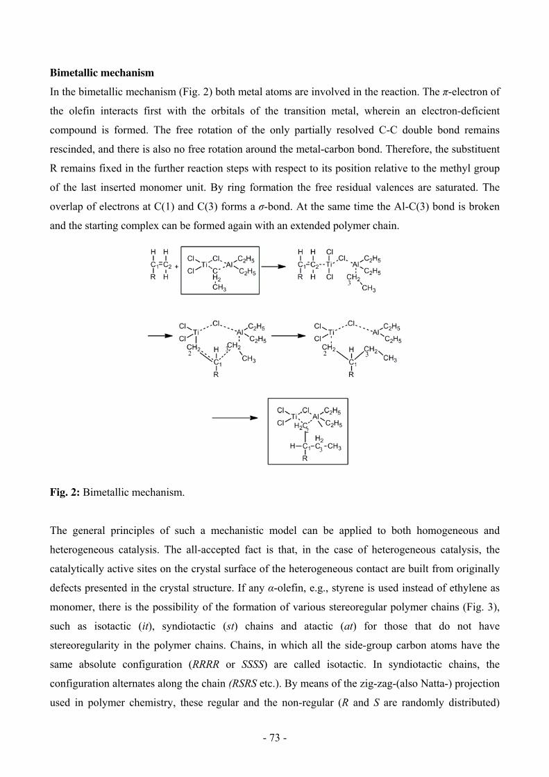
- 73 -

Bimetallic mechanism

In the bimetallic mechanism (Fig. 2) both metal atoms are involved in the reaction. The π-electron of

the olefin interacts first with the orbitals of the transition metal, wherein an electron-deficient

compound is formed. The free rotation of the only partially resolved C-C double bond remains

rescinded, and there is also no free rotation around the metal-carbon bond. Therefore, the substituent

R remains fixed in the further reaction steps with respect to its position relative to the methyl group

of the last inserted monomer unit. By ring formation the free residual valences are saturated. The

overlap of electrons at C(1) and C(3) forms a σ-bond. At the same time the Al-C(3) bond is broken

and the starting complex can be formed again with an extended polymer chain.

Fig. 2: Bimetallic mechanism.

The general principles of such a mechanistic model can be applied to both homogeneous and

heterogeneous catalysis. The all-accepted fact is that, in the case of heterogeneous catalysis, the

catalytically active sites on the crystal surface of the heterogeneous contact are built from originally

defects presented in the crystal structure. If any α-olefin, e.g., styrene is used instead of ethylene as

monomer, there is the possibility of the formation of various stereoregular polymer chains (Fig. 3),

such as isotactic (it), syndiotactic (st) chains and atactic (at) for those that do not have

stereoregularity in the polymer chains. Chains, in which all the side-group carbon atoms have the

same absolute configuration (RRRR or SSSS) are called isotactic. In syndiotactic chains, the

configuration alternates along the chain (RSRS etc.). By means of the zig-zag-(also Natta-) projection

used in polymer chemistry, these regular and the non-regular (R and S are randomly distributed)

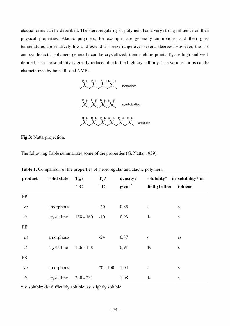
- 74 -

atactic forms can be described. The stereoregularity of polymers has a very strong influence on their

physical properties. Atactic polymers, for example, are generally amorphous, and their glass

temperatures are relatively low and extend as freeze-range over several degrees. However, the iso-

and syndiotactic polymers generally can be crystallized; their melting points Tm are high and well-

defined, also the solubility is greatly reduced due to the high crystallinity. The various forms can be

characterized by both IR- and NMR.

Fig 3: Natta-projection.

The following Table summarizes some of the properties (G. Natta, 1959).

Table 1. Comparison of the properties of stereoregular and atactic polymers.

product solid state Tm /

° C

Tg /

° C

density /

g·cm-3

solubility* in

diethyl ether

solubility* in

toluene

PP

at amorphous -20 0,85 s ss

it crystalline 158 - 160 -10 0,93 ds s

PB

at amorphous -24 0,87 s ss

it crystalline 126 - 128 0,91 ds s

PS

at amorphous 70 - 100 1,04 s ss

it crystalline 230 - 231 1,08 ds s

* s: soluble; ds: difficultly soluble; ss: slightly soluble.

- 75 -

1.3 Industrially important polymers prepared via coordinative polymerization

HDPE, high density polyethylene

Hostalen (Hoechst), Marlex (Phillips)

vessels, bags, sheets, dishes, disposable products, cable sheathing, insulators, hip joints, ...

it-PP, it-polypropylen

Hostalen PP (Hoechst), Novolen (BASF)

temperature-resistant containers, vessels, automotive, upholstery, ...

it-PB, it-poly-l-butene

tear-resistant films, pipes, ...

poly-4-methyl-l-pentene

TPX (Mitsui)

electrical and lighting industry, temperature resistant (mp 240 ° C), medical applications

trans-1,4-polyisoprene

golf balls, medical applications (for example shoe inserts)

cis-1,4-polyisoprene und -butadiene

rubber and tire industry

2 Experimental produce



the experiment is carried out, read the MSDS sheets for all the chemicals used in this laboratory and

be familiar with their safe handling. The instructions of the teaching assistant must be followed at all

times. Especially the following points are relevant:

1. Wearing of suitable protective clothing (protective goggles, glove, laboratory coat, etc.)


shower, first aid boxes, etc.), exit

3. Controlled disposal of toxic substances in compliance with legal regulations

4. Strict ban on eating, drinking and fuming in the laboratory

- 76 -

The greatest possible care must be exercised when working with organoaluminum compounds, since

they ignite very easily on contact with air and water. All operations must, therefore, be carried out

with the complete exclusion of air and moisture and pipettes must be flushed with nitrogen.

Moreover, these substances cause wounds that are slow to heal, so that the wearing of safety goggles

is mandatory and all contact with the skin must be avoided. The pipettes are cleaned as follows: after

all organoaluminum have been run out, the pipette is filled with ether and allowed to drain again. It is

then washed with isopropanol/HCl solvents.

2.2 Chemicals and equipment

Chemicals: heptane abs., triisobutylaluminium (25% in hexane), TiCl4 (caution!), styrene (freshly

distilled), 2-propanol, methanolic HCl (ca. 10%), methanol, methyl ethyl ketone (MEK), toluene.

Equipment: Gas purification system, Schlenk line with pressure relief valve, 500 mL three-neck flask

with gas introduction, KPG-stirrer, dropping funnel with pressure balance and

three-way valve, thermometer, oil bath with temperature sensor, hotplate, extraction flask with reflux

condenser and heating mantle, heating gun, vacuum desiccator (heatable), vacuum pump, N2-

cylinder with pressure reducer.

2.3 Experiment

The apparatus is evacuated (vacuum pump, slightly heated (heat gun) and filled with N2. After

cooling down the apparatus, 50 mL of absolute heptane are added with the aid of a dropping funnel

to the flask. Under a nitrogen atmosphere 1.0 mL of TiCl4 is added by a syringe and then 25 mL of

the aluminumalkyl-solution are added drop wise over a period of 20 minutes. Since the reaction of

the two catalyst is highly exothermic, an external cooling may be necessary. After approximately 10

minutes “aging time” of the catalyst, 25 mL styrene are added to the solution at once. The reaction

mixture is heated up to 75 °C (inside temperature) for 3-4 hours. After the mixture is cooled to room

temperature, the polymerization is stopped by adding 20 mL of 2-propanol under N2 and then

100 mL of 2-propanolic HCl subsequently (thorough mixing by vigorous stirring required). The

polymer is filtered off and washed thoroughly with methanol. The crude product is boiled under

reflux with 80 mL of methyl ethyl ketone, and then portion wise 30 mL of toluene are added and

extracted for 5 hours. The residue is first decanted and then sucked off with a coarse frit. After

washing with methyl ethyl ketone, the polymer is dried at 60 ° C in a vacuum desiccator. Both the

yield of it polystyrene and the melting range are to be determinated.

3 Questions about coordinative polymerization

- 77 -

1. Why is the extraction with MEK and toluene necessary?

2. What are the molar concentrations of the catalyst components in the reaction mixture?

Calculate the ratio Ti:styrene!

3. What is the difference between Fischer-projection and Natta-(Zig-Zag-) projection?

4. What is the difference between low and high pressure PE? Physically? Chemically?

5. What is meant by a 3rd-generation Ziegler catalyst?

6. Why can vinyl ether not be coordinative polymerized by TiCl4/Et3Al?

7. Structures of HDPE, LDPE, LLDPE, it-PP, st-PP, PB, trans-1,4-polyisoprene,

poly(4-methyl-1-pentene), cis-1,4-polybutadiene?

- 78 -

II Ring-Opening Metathesis Polymerization (ROMP)

Task

Polymerization of norbornene derivatives using the metathesis reaction and a transition metal

alkylidene catalyst.

Literature

1. R. H. Grubbs (Ed.) Handbook of Metathesis, Wiley-VCH, Weinheim, (2003)

2. M. Chanda, Introduction to Polymer Science and Chemistry: A Problem Solving Approach, CRC Press Inc.,

(2006)

3. F. J. David, Polymer Chemistry: A Practical Approach, Oxford University Press, (2004)

4. P. W. N. M van Leeuwen, Homogeneous Catalysts: Activity, Stability, Deactivation, Wiley-VCH, Weinheim,

(2011)

5. M. R. Buchmeiser, Chem. Rev. (2000), 100, 1565

Content

1. Introduction

2. Mechanism

3. Experimental part

4. Chemicals, equipment and safety

5. Experiment

6. Questions

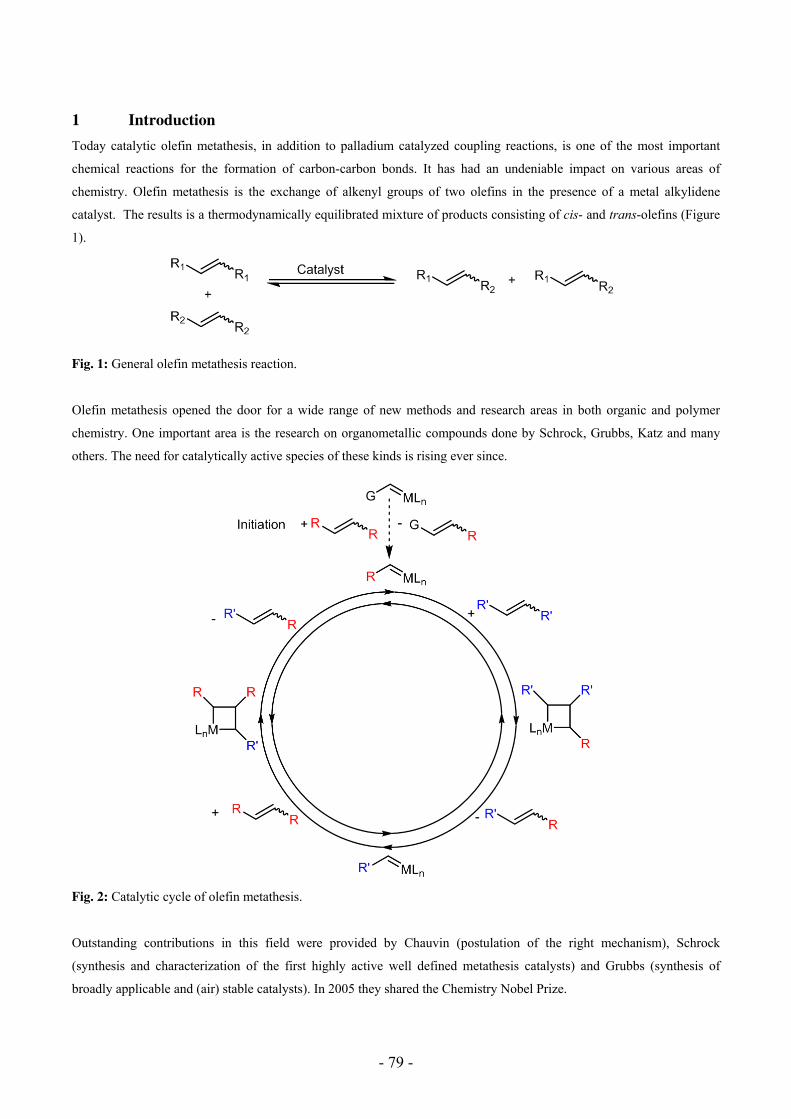
- 79 -

1 Introduction

Today catalytic olefin metathesis, in addition to palladium catalyzed coupling reactions, is one of the most important

chemical reactions for the formation of carbon-carbon bonds. It has had an undeniable impact on various areas of

chemistry. Olefin metathesis is the exchange of alkenyl groups of two olefins in the presence of a metal alkylidene

catalyst. The results is a thermodynamically equilibrated mixture of products consisting of cis- and trans-olefins (Figure

1).

Fig. 1: General olefin metathesis reaction.

Olefin metathesis opened the door for a wide range of new methods and research areas in both organic and polymer

chemistry. One important area is the research on organometallic compounds done by Schrock, Grubbs, Katz and many

others. The need for catalytically active species of these kinds is rising ever since.

Fig. 2: Catalytic cycle of olefin metathesis.

Outstanding contributions in this field were provided by Chauvin (postulation of the right mechanism), Schrock

(synthesis and characterization of the first highly active well defined metathesis catalysts) and Grubbs (synthesis of

broadly applicable and (air) stable catalysts). In 2005 they shared the Chemistry Nobel Prize.

- 80 -

In 1971, Y. Chauvin postulated that the olefin adds to the metal carbon double bond via a [2+2] cycloaddition. The

resulting intermediate is a metalla-cyclobutane species, which reacts to the product olefin and a new metal alkylidene via

a [2+2] cycloreversion. All steps in this reaction, in principle, are reversible. Thus, the product can be transformed back

to the starting material. Therefore, a driving force is needed to achieve high conversions and constantly shift the

equilibrium to the product side. This is illustrated in detail in Figure 2.

First observations of this kind of reactions were made in the 1950s when strange side products occured in the

polymerisation of ethylene in the presence of various metals. In early attempts, compounds like MoO3, WCl6, WOCl4 or

Re2O7 were used to selectively catalyze olefin metathesis. In addition, an alkylating agent had to be present (e.g., SnR4,

AlR3, etc.). These systems were highly active (but not selective). Another striking disadvantage was that they were

relatively short living and sensitive for impurities containing functional groups. In many cases, the real catalytically

active species remains unknown until today.

In 1964 Fischer synthesized the first metal-carbon double bond (carbene). The so called Fischer-carbenes are stabilized

by π-donors (Figure 3). Thus, these carbenes have a singlet configuration.

Fig. 3: Fischer-Carbene.

In 1974 Schrock prepaired the first metal-carbene without neighboring π-donors and with a transition metal in its highest

oxidation state. His alkylidenes (Figure 4) differ from Fischer-carbenes in that they possess a triplet configuration of the

metal carbon bond. Schrock synthesized complex 2 (Figure 4) by treating tantalum pentachloride with neopentyl lithium.

Fig. 4: First examples of a Schrock-carbene (alkylidene).

Through α-H-abstraction one equivalent of neopentane is lost and the new alkylidene forms. Schrock consequentially

recognized the unstable character of pentaalkyl substituted tantalum and proposed the formation of alkylidenes by this

mechanism. Over the years new and more active and stable catalysts were prepaired with great effort (Schrocks catalysts,

Figure 5). Grubbs made the invention of air (bench-top) stable rutheniumcarbenes (Figure 6), which set a new landmark

in the applicability of these catalysts. They are made by oxidation of Ru(II)-precursors. They complement to Schrocks

catalysts in their properties, because in general they are less active but also less sensitive. First and foremost they are

more stable to protic functional groups like alcohols or water. Schrock-alkylidenes in return have a better tolerance

towards functional groups containing sulfur, nitrogen or phosphorus.

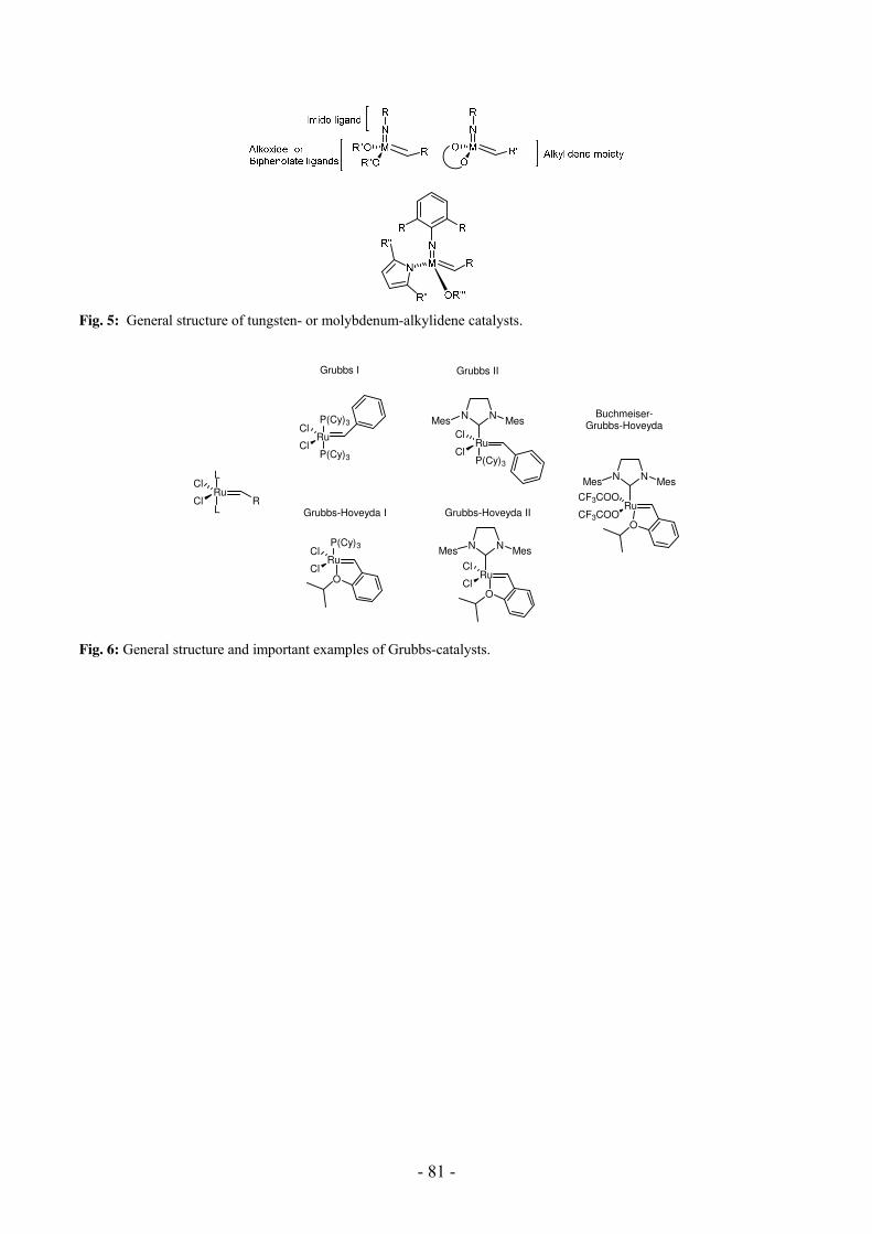
- 81 -

Fig. 5: General structure of tungsten- or molybdenum-alkylidene catalysts.

RuR

Cl

Cl

L

L

Ru

P(Cy)3

P(Cy)3

Cl

Cl RuCl

ClP(Cy)3

NNMesMes

Grubbs I

Ru

P(Cy)3Cl

ClO Ru

Cl

ClO

NNMesMes

Grubbs-Hoveyda I

Grubbs II

Grubbs-Hoveyda IIRu

CF3COO

CF3COOO

NNMesMes

Buchmeiser-Grubbs-Hoveyda

Fig. 6: General structure and important examples of Grubbs-catalysts.

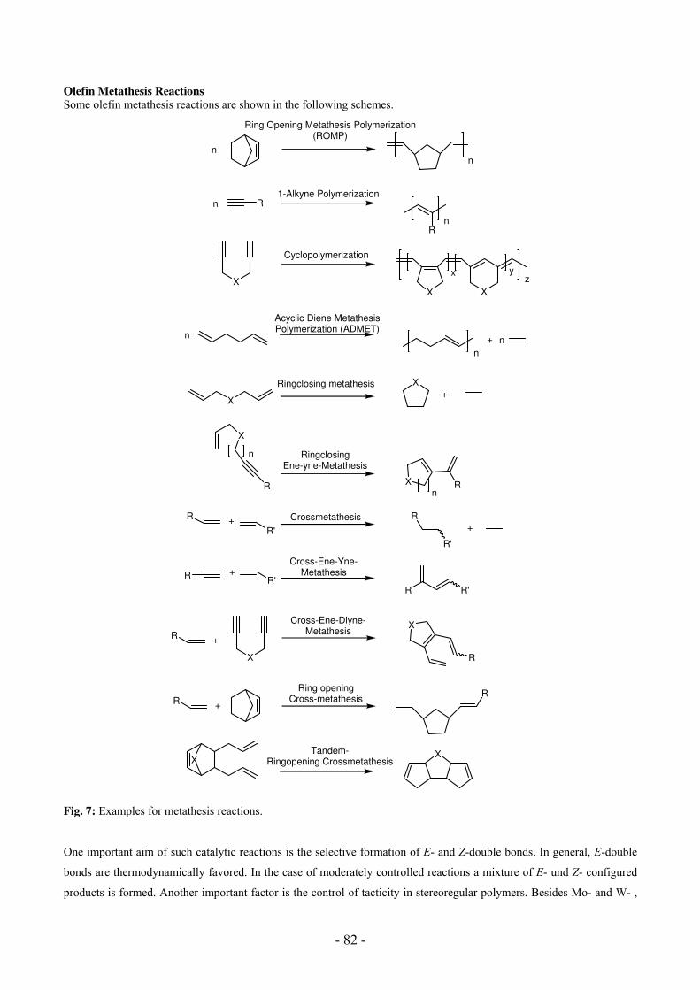
- 82 -

Olefin Metathesis Reactions

Some olefin metathesis reactions are shown in the following schemes.

nn

Rn

Rn

XX X

x yz

Ring Opening Metathesis Polymerization (ROMP)

1-Alkyne Polymerization

Cyclopolymerization

nn

n

+

Acyclic Diene Metathesis Polymerization (ADMET)

R

R'+ R

R'

+Crossmetathesis

R +R'

R R'

Cross-Ene-Yne-Metathesis

X

R

n

X Rn

RingclosingEne-yne-Metathesis

X

R +

X

R

Cross-Ene-Diyne-Metathesis

R +

RRing opening

Cross-metathesis

XTandem-

Ringopening CrossmetathesisX

X

Ringclosing metathesis X

+

Fig. 7: Examples for metathesis reactions.

One important aim of such catalytic reactions is the selective formation of E- and Z-double bonds. In general, E-double

bonds are thermodynamically favored. In the case of moderately controlled reactions a mixture of E- und Z- configured

products is formed. Another important factor is the control of tacticity in stereoregular polymers. Besides Mo- and W- ,

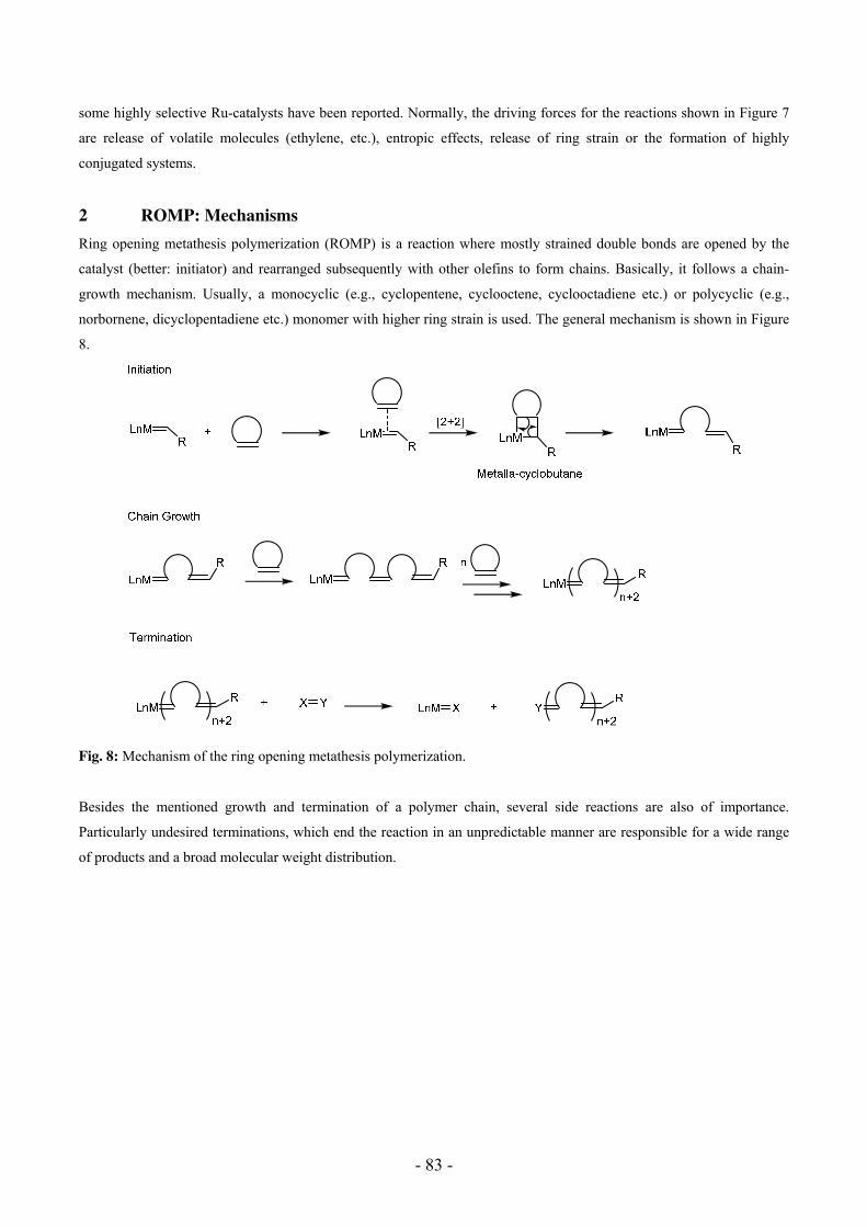
- 83 -

some highly selective Ru-catalysts have been reported. Normally, the driving forces for the reactions shown in Figure 7

are release of volatile molecules (ethylene, etc.), entropic effects, release of ring strain or the formation of highly

conjugated systems.

2 ROMP: Mechanisms

Ring opening metathesis polymerization (ROMP) is a reaction where mostly strained double bonds are opened by the

catalyst (better: initiator) and rearranged subsequently with other olefins to form chains. Basically, it follows a chain-

growth mechanism. Usually, a monocyclic (e.g., cyclopentene, cyclooctene, cyclooctadiene etc.) or polycyclic (e.g.,

norbornene, dicyclopentadiene etc.) monomer with higher ring strain is used. The general mechanism is shown in Figure

8.

Fig. 8: Mechanism of the ring opening metathesis polymerization.

Besides the mentioned growth and termination of a polymer chain, several side reactions are also of importance.

Particularly undesired terminations, which end the reaction in an unpredictable manner are responsible for a wide range

of products and a broad molecular weight distribution.

- 84 -

Fig. 9: Undesired terminations that can occur in ROMP.

RR

R R

n/2

R R

n/2

R R

RR

R R

n/2

R R

n/2

R R

R

R

[cat.]

n

cis-syndio tactic

cis-iso tactic

trans-iso tactic

trans-syndio tactic

Fig. 10: Formation of different polymer structures of poly-Norbornadienenes through ROMP.

The determining factor for the physical properties of polymers is their microstructure. For instance, the ROMP of

substituted norbornadienenes can produce four different regular structures of the polymer or a mixture of them. Cis- and

trans- double bonds as well as iso- and syndiotactic incorporation of the five membered repeat units is possible. With

chiral substrates, the microstructure can be even more complicated.

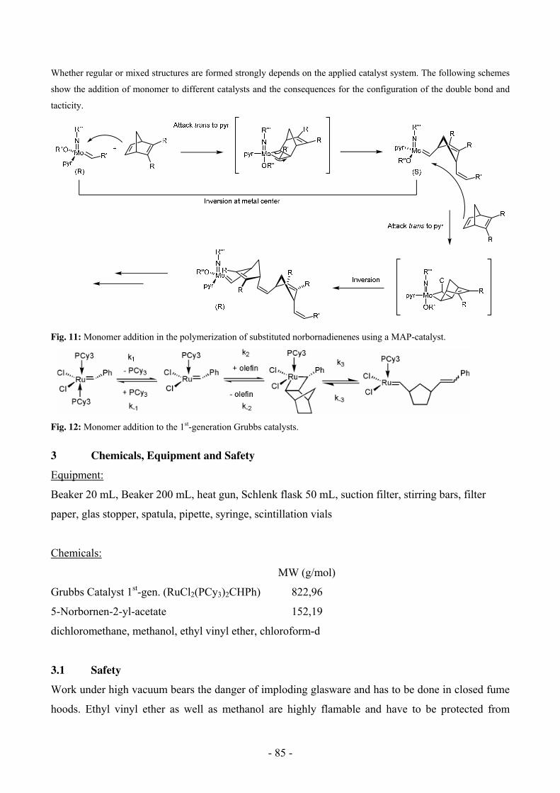
- 85 -

Whether regular or mixed structures are formed strongly depends on the applied catalyst system. The following schemes

show the addition of monomer to different catalysts and the consequences for the configuration of the double bond and

tacticity.

Fig. 11: Monomer addition in the polymerization of substituted norbornadienenes using a MAP-catalyst.

Fig. 12: Monomer addition to the 1st-generation Grubbs catalysts.

3 Chemicals, Equipment and Safety

Equipment:

Beaker 20 mL, Beaker 200 mL, heat gun, Schlenk flask 50 mL, suction filter, stirring bars, filter

paper, glas stopper, spatula, pipette, syringe, scintillation vials

Chemicals:

MW (g/mol)

Grubbs Catalyst 1st-gen. (RuCl2(PCy3)2CHPh) 822,96

5-Norbornen-2-yl-acetate 152,19

dichloromethane, methanol, ethyl vinyl ether, chloroform-d

3.1 Safety

Work under high vacuum bears the danger of imploding glasware and has to be done in closed fume

hoods. Ethyl vinyl ether as well as methanol are highly flamable and have to be protected from

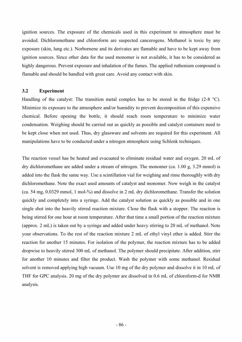
- 86 -

ignition sources. The exposure of the chemicals used in this experiment to atmosphere must be

avoided. Dichloromethane and chloroform are suspected cancerogens. Methanol is toxic by any

exposure (skin, lung etc.). Norbornene and its derivates are flamable and have to be kept away from

ignition sources. Since other data for the used monomer is not available, it has to be considered as

highly dangerous. Prevent exposure and inhalation of the fumes. The applied ruthenium compound is

flamable and should be handled with great care. Avoid any contact with skin.

3.2 Experiment

Handling of the catalyst: The transition metal complex has to be stored in the fridge (2-8 °C).

Minimize its exposure to the atmosphere and/or humidity to prevent decomposition of this expensive

chemical. Before opening the bottle, it should reach room temperature to minimize water

condensation. Weighing should be carried out as quickly as possible and catalyst containers need to

be kept close when not used. Thus, dry glassware and solvents are required for this experiment. All

manipulations have to be conducted under a nitrogen atmosphere using Schlenk techniques.

The reaction vessel has be heated and evacuated to eliminate residual water and oxygen. 20 mL of

dry dichloromethane are added under a stream of nitrogen. The monomer (ca. 1.00 g, 3.29 mmol) is

added into the flask the same way. Use a scintillation vial for weighing and rinse thoroughly with dry

dichloromethane. Note the exact used amounts of catalyst and monomer. Now weigh in the catalyst

(ca. 54 mg, 0.0329 mmol, 1 mol-%) and dissolve in 2 mL dry dichloromethane. Transfer the solution

quickly and completely into a syringe. Add the catalyst solution as quickly as possible and in one

single shot into the heavily stirred reaction mixture. Close the flask with a stopper. The reaction is

being stirred for one hour at room temperature. After that time a small portion of the reaction mixture

(approx. 2 mL) is taken out by a syringe and added under heavy stirring to 20 mL of methanol. Note

your observations. To the rest of the reaction mixture 2 mL of ethyl vinyl ether is added. Stirr the

reaction for another 15 minutes. For isolation of the polymer, the reaction mixture has to be added

dropwise to heavily stirred 300 mL of methanol. The polymer should precipitate. After addition, stirr

for another 10 minutes and filter the product. Wash the polymer with some methanol. Residual

solvent is removed applying high vacuum. Use 10 mg of the dry polymer and dissolve it in 10 mL of

THF for GPC analysis. 20 mg of the dry polymer are dissolved in 0.6 mL of chloroform-d for NMR

analysis.

- 87 -

4 Questions

1. What was the visual difference you observed when precipitating the polymer for the first

and second time? Explain.

2. What is ethyl vinyl ether used for in this experiment and what is being formed after addition?

Write down the reaction equations for the reactions in this experiment and explain why

ethyl vinyl ether is a good candidate for the needed purpose. Would 1-pentene be an

alternative? Why/(not)?

3. Why has the catalyst solution to be added as quickly as possible? Clarify the role of

temperature, mixing and concentration of monomer solution in this regard.

4. Calculate the theoretical values for molecular weight of the synthesized polymer chains.

Compare them to the experimentally found values determined by GPC analysis. Explain any

deviations. Why, in general, can an experiment deliver much higher or smaller values

compared to the theoretical ones?

5. Do you see any possible way to reuse the catalyst? What is necessary to accomplish this?

6. Name some simple ways to prepare (in this experiment) polymers with higher solubility?

Name factors which play a crucial role.

7. Which influences can an applied catalyst system have on the reaction process and the

product? Why do expensive and sensitive systems still play an important role?

8. What is the striking structural feature of transition metal alkylidene complexes? What

significant difference would you expect from the NMR spectrum of a propagating species to

the parent catalyst?

9. Assign the observed signals you see in the 1H-NMR of the polymer and explain the

differences to the spectrum of the monomer.

88

Experiment 6: Emulsion Polymerization

Objective

Styrene is polymerized in an emulsion using dodecyl hydrogen sulfate sodium salt as an emulsifier and potassium persulfate as the initiator. Samples are drawn from the reactant solution in regular intervals in order to generate diagrams of the conversion as well as the reaction rate versus the reaction time.

References

1) H.‐G. Elias, Makromoleküle Bd. 1, Edition 6, Wiley‐VCH Verlag, Weinheim, 1999

2) P. J. Flory, Principles of Polymer Chemistry, Cornell, University Press, Ithaca, 1953

3) B. Tieke, Makromolekulare Chemie, Edition 2, Wiley‐VCH Verlag, Weinheim, 2005

4) W. V. Smith, H. Ewart, J. Chem. Phys. 16(6), 592 (1948)

5) W. D. Harkins, J. Am. Chem. Soc. 69, 1428 (1947)

Content

1. Theoretical Background

2. Experimental Part

3. Questions

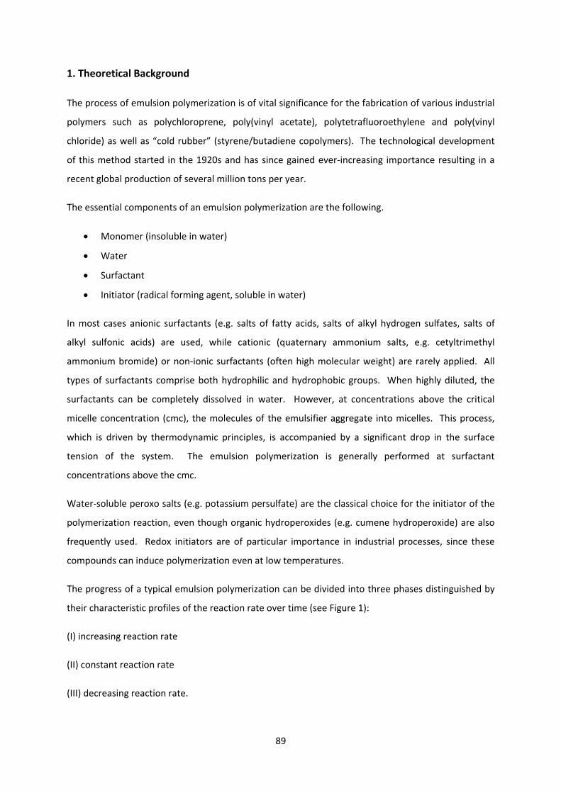
89


The process of emulsion polymerization is of vital significance for the fabrication of various industrial

polymers such as polychloroprene, poly(vinyl acetate), polytetrafluoroethylene and poly(vinyl

chloride) as well as “cold rubber” (styrene/butadiene copolymers). The technological development

of this method started in the 1920s and has since gained ever‐increasing importance resulting in a

recent global production of several million tons per year.

The essential components of an emulsion polymerization are the following.

Monomer (insoluble in water)

Water

Surfactant

Initiator (radical forming agent, soluble in water)

In most cases anionic surfactants (e.g. salts of fatty acids, salts of alkyl hydrogen sulfates, salts of

alkyl sulfonic acids) are used, while cationic (quaternary ammonium salts, e.g. cetyltrimethyl

ammonium bromide) or non‐ionic surfactants (often high molecular weight) are rarely applied. All

types of surfactants comprise both hydrophilic and hydrophobic groups. When highly diluted, the

surfactants can be completely dissolved in water. However, at concentrations above the critical

micelle concentration (cmc), the molecules of the emulsifier aggregate into micelles. This process,

which is driven by thermodynamic principles, is accompanied by a significant drop in the surface

tension of the system. The emulsion polymerization is generally performed at surfactant

concentrations above the cmc.

Water‐soluble peroxo salts (e.g. potassium persulfate) are the classical choice for the initiator of the

polymerization reaction, even though organic hydroperoxides (e.g. cumene hydroperoxide) are also

frequently used. Redox initiators are of particular importance in industrial processes, since these

compounds can induce polymerization even at low temperatures.

The progress of a typical emulsion polymerization can be divided into three phases distinguished by

their characteristic profiles of the reaction rate over time (see Figure 1):

(I) increasing reaction rate

(II) constant reaction rate

(III) decreasing reaction rate.

Figure 1

transitio

Figure 1: D

Harkin a

processe

initial re

At the b

~4.3 nm

of mono

emulsifie

micelles

formed

the mice

number

emulsion

monome

no relev

polymer

monome

monome

limited

transform

of the re

1 further ill

on between t

Development o

s well as Sm

es occurring

servations, t

beginning of

) as well as m

omer, howev

er (see Figu

by diffusion

in this proce

elles. Howev

(~1010 per c

n) present in

er droplets a

vance due t

rization the

er molecules

er droplets

conditions).

m into so‐ca

eaction and t

ustrates tha

the first and

of the reaction

ith and Ewa

at a molec

the essential

f the polyme

micelles swo

ver, is initially

ure 2). Mon

n. The water

ess can, in p

ver, the reac

cm3 emulsio

n the system

and the mice

o the very

monomer i

s. This effec

leading to a

As a resu

alled latex pa

the reaction

at the surfa

the second p

rate (vp) and th

rts were the

ular level du

aspects of t

erization rea

ollen by mon

y bound in m

nomer mole

r‐soluble init

rinciple, star

ction is far le

n) is signific

m, which corr

elles. Polym

low concen

is depleted

ct is compen

a constant m

lt of the on

articles. Mor

rate increase

90

ace tension

phase.

he surface tens

first to prop

uring an em

these concep

action, the s

nomer incorp

monomer dr

ecules can b

tiator decom

rt a polymer

ess likely to

cantly lower

responds to

merization in

ntration of t

within the

nsated by mo

monomer co

ngoing polym

re and more

es.

of the syst

sion (γ) as a fun

pose correct

mulsion polym

pts are widel

system conta

poration (dia

oplets (diam

be transferre

mposes in the

rization eithe

begin within

than the am

a surface ar

the aqueou

the water‐in

micelles, w

onomers diff

oncentration

merization r

e polymer ch

em drastica

nction of the po

interpretatio

merization [4

y accepted t

ains “empty

ameter ~5 nm

meter ~1000

ed from the

e aqueous ph

er in the mo

n the monom

mount of mic

rea ratio of ~

s phase, on

soluble! mo

which each

fusing into t

in the nano

reaction, the

ains are star

ally increase

olymerization t

ons of the un

4, 5]. Desp

today.

y” micelles (

m). The vast

nm) stabilize

ese droplets

hase and the

nomer drop

mer droplets

celles (~1018

~1:1000 betw

the other ha

onomer. Du

contain aro

the micelles

o‐reactors (d

e micelles g

rted in this f

es at the

time (t).

nderlying

ite some

diameter

t amount

ed by the

into the

e radicals

lets or in

s, as their 8 per cm3

ween the

and, is of

uring the

ound 100

from the

diffusion‐

grow and

irst stage

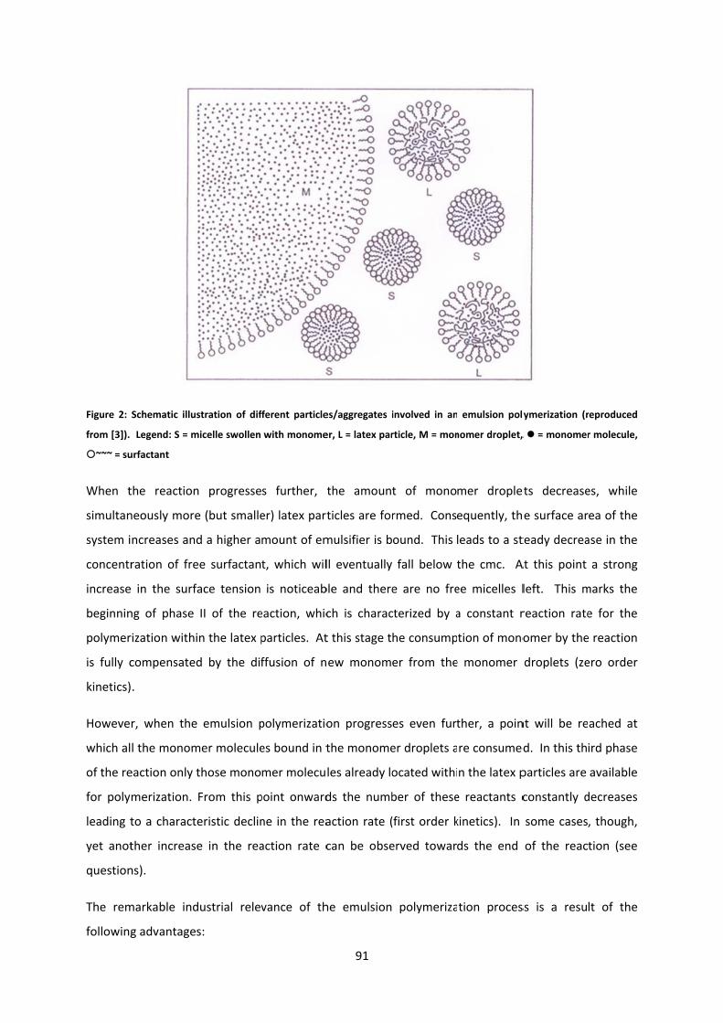
Figure 2:

from [3]).

~~~ = su

When t

simultan

system i

concentr

increase

beginnin

polymer

is fully c

kinetics)

Howeve

which al

of the re

for poly

leading t

yet anot

question

The rem

following

Schematic illu

Legend: S = m

urfactant

the reaction

neously more

ncreases an

ration of fre

e in the surf

ng of phase

rization withi

compensate

.

r, when the

l the monom

eaction only

merization.

to a charact

ther increas

ns).

markable ind

g advantage

stration of dif

micelle swollen

n progresse

e (but smalle

d a higher a

ee surfactan

face tension

II of the re

in the latex p

d by the dif

e emulsion p

mer molecule

those mono

From this p

teristic declin

e in the rea

dustrial relev

s:

fferent particle

with monome

s further, t

er) latex part

mount of em

t, which wil

is noticeab

eaction, whic

particles. At

ffusion of n

polymerizatio

es bound in t

mer molecu

point onward

ne in the rea

action rate c

vance of th

91

es/aggregates i

er, L = latex par

the amoun

ticles are for

mulsifier is b

ll eventually

ble and there

ch is charac

t this stage t

ew monom

on progress

the monome

les already lo

ds the numb

action rate (

can be obse

he emulsion

involved in an

rticle, M = mon

t of mono

rmed. Cons

ound. This

fall below t

e are no fre

cterized by a

he consump

er from the

es even furt

er droplets a

ocated withi

ber of these

(first order k

erved towar

polymeriza

emulsion poly

nomer droplet,

mer drople

equently, th

leads to a st

the cmc. A

ee micelles l

a constant r

tion of mono

e monomer

ther, a poin

re consumed

n the latex p

e reactants c

kinetics). In

ds the end

tion proces

ymerization (r

, = monomer

ets decrease

e surface ar

teady decrea

At this point

left. This m

reaction rate

omer by the

droplets (ze

nt will be re

d. In this th

particles are

constantly d

some cases

of the reac

ss is a resu

reproduced

r molecule,

es, while

ea of the

ase in the

a strong

marks the

e for the

e reaction

ero order

ached at

ird phase

available

decreases

, though,

tion (see

lt of the

92

a) The aqueous phase enables temperature regulation during the polymerization reaction.

b) Redox initiators can be applied, which enable polymerization reactions to proceed at comparably

low temperatures, yet keeping the reaction rate relatively high.

c) High degrees of polymerization can be achieved due to the small probability of chain termination.

This can be further regulated by the controlled addition of chain transfer agents.

d) Remaining monomer can be removed by steam distillation.

e) The obtained latex can be directly subjected to further applications (paints, glues, coatings).

On the downside, however, a frequently problematic extraction of the emulsifier as well as the

potentially high degree of branching of the polymer chains have to be taken into account as major

disadvantages of the method.

Kinetics and Mechanism

A hallmark of the emulsion polymerization process is that this method yields higher degrees of

polymerization than those accessible under comparable conditions in bulk or suspension

polymerization reactions. The kinetics and the mechanism of emulsion polymerization are,

therefore, distinct from other radical polymerization methods. The reaction rate vw(L) in an individual

latex particle is given by equation (1).

(1) [M][P*]k)(v Ww L

vw(L): reaction rate of the polymerization in the latex particle

kw: rate constant of the polymerization

[M]: concentration of monomer in the latex particle

[P*]: concentration of radicals in the latex particle

The measurable reaction rate vw of the entire reaction batch is represented by the sum of the

reaction rates in all isolated latex particles. Assuming a narrow size distribution of the latex particles

the reaction rate can be described as follows:

93

(2) A

wwN

nN[M]kv

vw: reaction rate of the polymerization

n: average number of free radicals per latex particle

N: number of latex particles per unit volume of the emulsion

NA: Avogadro constant

In equation (2), it is further assumed that the polymerization occurs exclusively within the latex

particles, i.e. there is no considerable amount of polymer forming either in the aqueous phase or in

the monomer droplets. For the determination of vW the factors included in equation (2) have to be

expressed as properties, which are experimentally accessible. This is particularly difficult in the case

of N and n. The most established quantitative model for the description of the kinetics and the

mechanism of the emulsion polymerization was derived by Smith and Ewart. It is particularly well‐

suited for systems showing a behavior consistent with the Harkin model.

The Harkin model is based on the following considerations: After a short phase of particle generation

(phase I) the reaction rate becomes constant in phase (II). Therefore, regarding the factors included

in equation (2), not only the monomer concentration [M] and the number of latex particles per unit

volume [N], but also the number of free radicals within the latex particles have to be constant.

However, according to the steady state approximation the number of these radicals will only remain

constant, when equal amounts of radicals are formed and consumed in a given period of time.

The following assumptions will be made: Once a radical is located within a latex particle, it cannot

leave this environment again. If a second radical enters the same latex particle, an immediate

recombination of the two will take place due to the small radius of the latex particle. An individual

latex particle, therefore, contains either one or no radical at any given time, corresponding to an

average number of radicals per latex particle of n = ½. With additional assumptions regarding the

number of latex particles equation (3) can be derived:

(3) 5

3

S5

2

A

ww [S])(a)N

σb(

2

1[M]kv

b: system constant in the range of 0.37‐0.53

σ: inflow/intake velocity of the radical into the latex particle

µ: constant volume increase of the latex particle

94

aS: surface area required by one surfactant molecule

[S]: concentration of the emulsifier

Combining all constant parameters included in equation (3) into a single constant K leads to a

simplified representation as given by equation (4):

(4) 5

3

w K[M]([S])v

On closer examination of equation (4) it becomes obvious, that the reaction rate of the emulsion

polymerization can be raised even without increasing the temperature, monomer concentration or

initiator concentration – simply by adding a higher amount of the surfactant.

The degree of polymerization Pn of a polymerization reaction is defined as the ratio between the sum

of all reaction rates associated with processes leading to an increase in the chain length and the sum

of reaction rates ascribed to those processes resulting in the termination of an individual chain. The

latter can occur either by direct termination or by chain transfer to monomer, solvent, or initiator

molecules (but not to polymer chains!).

(5) )v(v

vP

TA

wn

vA: sum of the reaction rates of all processes terminating the chain

vT: sum of the rates of all chain transfer reactions

As the concentration of the emulsifier directly influences vw, it also has an immediate effect on the

degree of polymerization. In contrast to all other radical polymerization processes, the

recombination of radical chain ends is inhibited in emulsion polymerization, since the chains exist in

isolated latex particles and are therefore effectively separated from each other.

Moreover, in its final stages the process of emulsion polymerization shows a behavior analogous to

the Norrish‐Trommsdorf effect, which is known from bulk polymerization. As a result, the reaction

rate and the degree of polymerization are comparably higher.

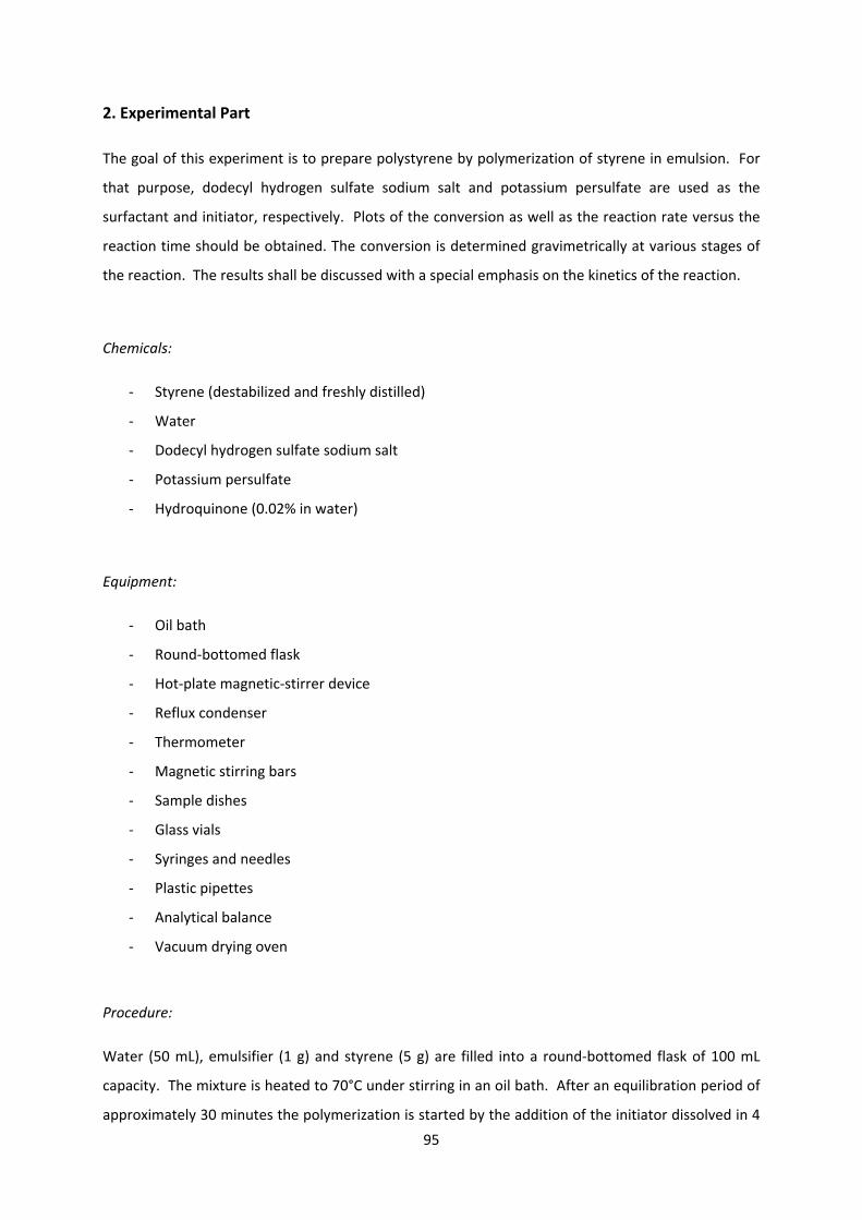
95


The goal of this experiment is to prepare polystyrene by polymerization of styrene in emulsion. For

that purpose, dodecyl hydrogen sulfate sodium salt and potassium persulfate are used as the

surfactant and initiator, respectively. Plots of the conversion as well as the reaction rate versus the

reaction time should be obtained. The conversion is determined gravimetrically at various stages of

the reaction. The results shall be discussed with a special emphasis on the kinetics of the reaction.

Chemicals:

‐ Styrene (destabilized and freshly distilled)

‐ Water

‐ Dodecyl hydrogen sulfate sodium salt

‐ Potassium persulfate

‐ Hydroquinone (0.02% in water)

Equipment:

‐ Oil bath

‐ Round‐bottomed flask

‐ Hot‐plate magnetic‐stirrer device

‐ Reflux condenser

‐ Thermometer

‐ Magnetic stirring bars

‐ Sample dishes

‐ Glass vials

‐ Syringes and needles

‐ Plastic pipettes

‐ Analytical balance

‐ Vacuum drying oven

Procedure:

Water (50 mL), emulsifier (1 g) and styrene (5 g) are filled into a round‐bottomed flask of 100 mL

capacity. The mixture is heated to 70°C under stirring in an oil bath. After an equilibration period of

approximately 30 minutes the polymerization is started by the addition of the initiator dissolved in 4

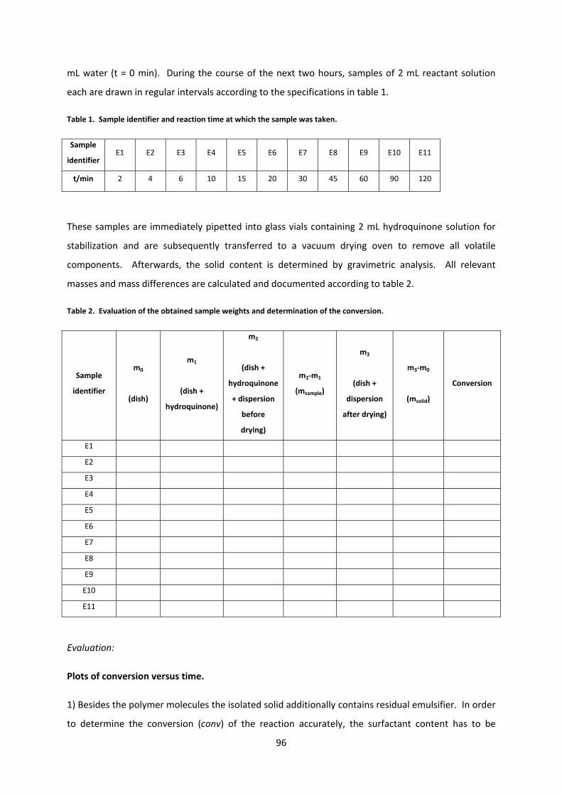
96

mL water (t = 0 min). During the course of the next two hours, samples of 2 mL reactant solution

each are drawn in regular intervals according to the specifications in table 1.

Table 1. Sample identifier and reaction time at which the sample was taken.

Sample

identifier E1 E2 E3 E4 E5 E6 E7 E8 E9 E10 E11

t/min 2 4 6 10 15 20 30 45 60 90 120

These samples are immediately pipetted into glass vials containing 2 mL hydroquinone solution for

stabilization and are subsequently transferred to a vacuum drying oven to remove all volatile

components. Afterwards, the solid content is determined by gravimetric analysis. All relevant

masses and mass differences are calculated and documented according to table 2.

Table 2. Evaluation of the obtained sample weights and determination of the conversion.

Sample

identifier

m0

(dish)

m1

(dish +

hydroquinone)

m2

(dish +

hydroquinone

+ dispersion

before

drying)

m2‐m1

(msample)

m3

(dish +

dispersion

after drying)

m3‐m0

(msolid)

Conversion

E1

E2

E3

E4

E5

E6

E7

E8

E9

E10

E11

Evaluation:

Plots of conversion versus time.

1) Besides the polymer molecules the isolated solid additionally contains residual emulsifier. In order

to determine the conversion (conv) of the reaction accurately, the surfactant content has to be

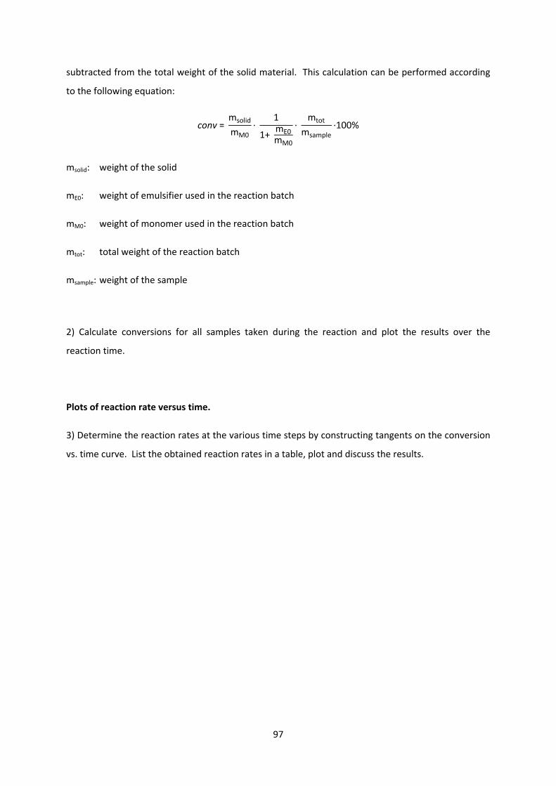
97

subtracted from the total weight of the solid material. This calculation can be performed according

to the following equation:

conv = msolid

mM0

· 1

1+ mE0

mM0

· mtot

msample

·100%

msolid: weight of the solid

mE0: weight of emulsifier used in the reaction batch

mM0: weight of monomer used in the reaction batch

mtot: total weight of the reaction batch

msample: weight of the sample

2) Calculate conversions for all samples taken during the reaction and plot the results over the

reaction time.

Plots of reaction rate versus time.

3) Determine the reaction rates at the various time steps by constructing tangents on the conversion

vs. time curve. List the obtained reaction rates in a table, plot and discuss the results.

98

3. Questions

1) Which effects can be potentially caused by the presence of oxygen traces in the emulsion? What

could be an explanation for another increase in the reaction rate during the final stages of the

polymerization (Take into account that the reaction is a radical polymerization)?

2) Why is the coagulation of latex particles inhibited?

3) What is the average radical concentration in the latex particles under the following assumptions?

The radicals reach the latex particles by diffusion. This process determines the reaction rate.

Whenever two radicals are located in the same latex particle they will recombine

immediately.

4) Describe the principle of a redox initiator and list a number of examples.

5) Compare the characteristics of emulsion polymerization and suspension polymerization. Name

further examples for technologically relevant polymerization procedures.

-99-

Experiment 7

Anionic Polymerization

Assignment

The concept of living anionic vinyl polymerization will be demonstrated by the block

copolymerization of styrene and isoprene with sec-butyllithium in toluene.

References

1) H.-G. Elias, An Introduction to Polymer Science, 1. Auflage, Wiley-VCH-Verlag,

Weinheim, 1997

2) M. Morton, Anionic Polymerization: Principles and Practice, Academic Press, New

York, 1983

Contents

1. Introduction

1.1 General Remarks

1.2. Anionic Polymerization

1.2.1. Initiation Reaction

1.2.2. Propagation Reaction


2.1. Anionic Polymerization of Styrene/Isoprene

2.2. Evaluation

3. Questions

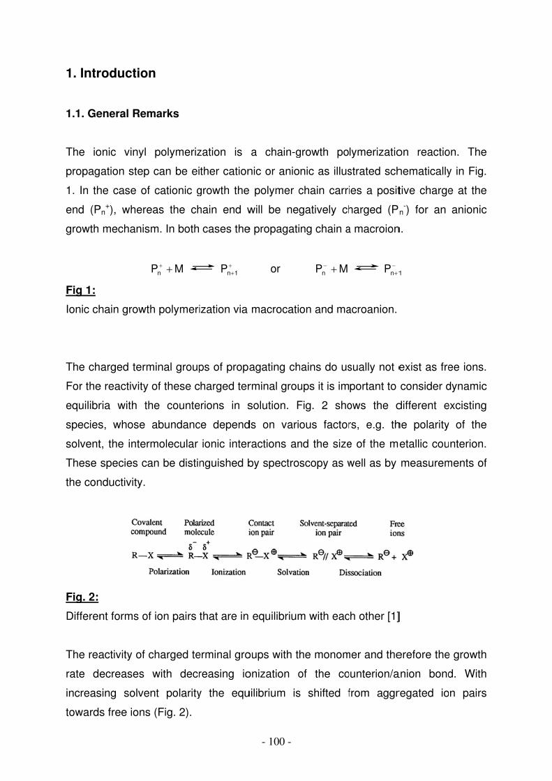
1. Intr

1.1. Ge

The io

propag

1. In th

end (P

growth

Fig 1:

Ionic ch

The ch

For the

equilibr

species

solvent

These

the con

Fig. 2:

Differen

The rea

rate de

increas

towards

roduction

eneral Rem

onic vinyl

ation step

he case of

Pn+), where

mechanis

hain growt

arged term

e reactivity

ria with th

s, whose

t, the inter

species ca

nductivity.

nt forms of

activity of c

ecreases

sing solve

s free ions

n

marks

polymeriz

can be ei

f cationic g

eas the ch

m. In both

P Mn

h polymeri

minal group

of these c

he counte

abundanc

rmolecular

an be distin

f ion pairs

charged te

with decr

nt polarity

s (Fig. 2).

zation is

ther cation

growth the

hain end w

cases the

Pn 1

ization via

ps of propa

charged ter

erions in s

ce depend

ionic inter

nguished b

that are in

erminal gro

reasing io

y the equ

- 100 -

a chain-g

nic or anio

polymer c

will be neg

e propagati

or

macrocati

agating ch

rminal grou

solution. F

ds on vari

ractions an

by spectro

equilibrium

oups with t

onization o

uilibrium is

growth po

nic as illus

chain carri

gatively ch

ng chain a

P Mn

on and ma

hains do us

ups it is im

Fig. 2 sho

ous factor

nd the size

scopy as w

m with eac

he monom

of the co

s shifted f

lymerizatio

strated sch

ies a posit

harged (Pn

a macroion

Pn 1

acroanion.

sually not e

portant to

ows the d

rs, e.g. th

e of the me

well as by

ch other [1]

mer and the

ounterion/a

from aggr

on reactio

hematically

tive charge

n-) for an

n.

1

exist as fre

consider d

different e

he polarity

etallic cou

measurem

]

erefore the

anion bond

regated io

on. The

y in Fig.

e at the

anionic

ee ions.

dynamic

excisting

y of the

nterion.

ments of

e growth

d. With

n pairs

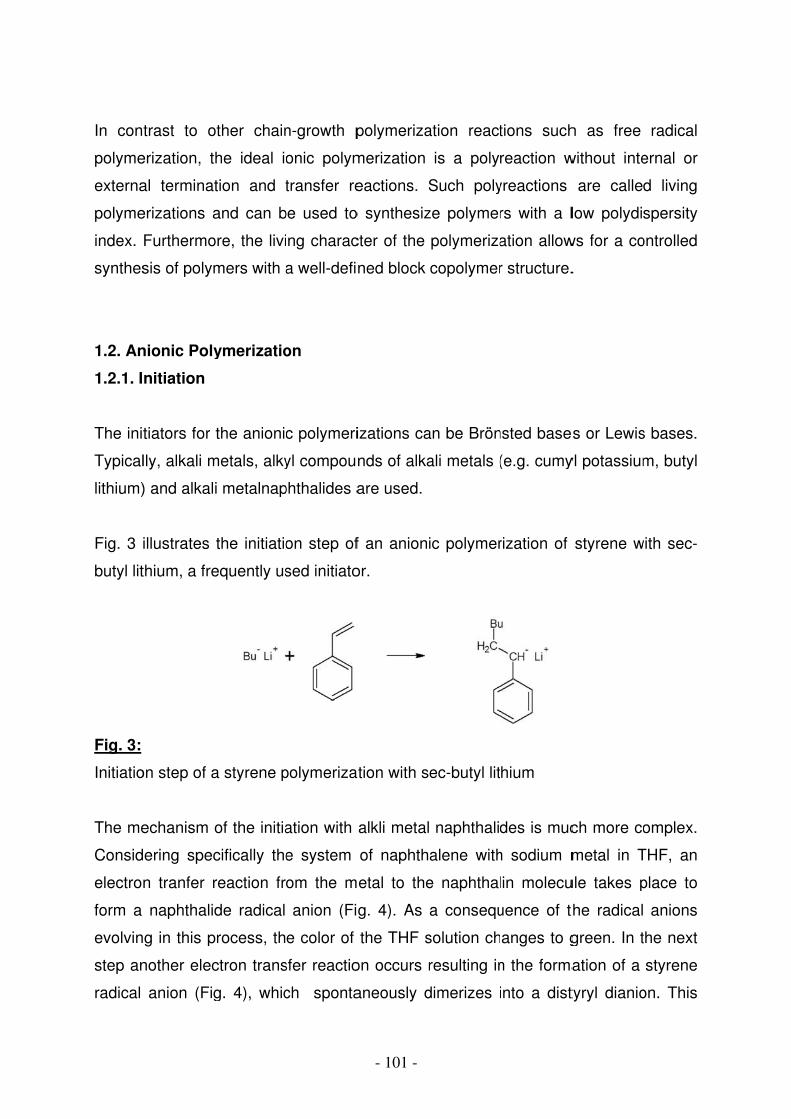
In con

polyme

externa

polyme

index.

synthes

1.2. An

1.2.1. I

The ini

Typical

lithium)

Fig. 3

butyl lit

Fig. 3:

Initiatio

The me

Consid

electro

form a

evolvin

step an

radical

trast to o

erization, t

al terminat

erizations a

Furthermo

sis of polym

nionic Poly

nitiation

tiators for

lly, alkali m

) and alkal

illustrates

thium, a fre

on step of a

echanism

ering spec

n tranfer r

naphthalid

g in this p

nother elec

anion (Fig

other chain

he ideal io

tion and t

and can b

ore, the livi

mers with a

ymerizatio

the anioni

metals, alky

i metalnap

the initiatio

equently us

a styrene p

of the initia

cifically the

reaction fr

de radical

process, th

ctron trans

g. 4), whic

n-growth p

onic polym

transfer re

be used to

ng charac

a well-defi

on

c polymeri

yl compoun

phthalides a

on step of

sed initiato

polymeriza

ation with

e system

om the m

anion (Fi

e color of

sfer reactio

ch sponta

- 101 -

polymeriza

merization

eactions. S

o synthesiz

cter of the

ned block

izations ca

nds of alka

are used.

f an anion

or.

tion with s

alkli metal

of naphth

etal to the

g. 4). As

the THF s

on occurs r

aneously d

ation react

is a poly

Such poly

ze polymer

polymeriza

copolymer

an be Brön

ali metals (

ic polymer

ec-butyl lit

naphthalid

alene with

e naphthal

a consequ

solution ch

resulting in

dimerizes i

tions such

reaction w

yreactions

rs with a l

ation allow

r structure.

nsted base

(e.g. cumy

rization of

hium

des is muc

h sodium m

lin molecu

uence of t

anges to g

n the forma

into a dist

h as free

without inte

are calle

low polydi

ws for a co

.

s or Lewis

yl potassium

styrene w

ch more co

metal in T

ule takes p

the radical

green. In t

ation of a

tyryl dianio

radical

ernal or

d living

spersity

ontrolled

s bases.

m, butyl

with sec-

omplex.

THF, an

place to

anions

the next

styrene

on. This

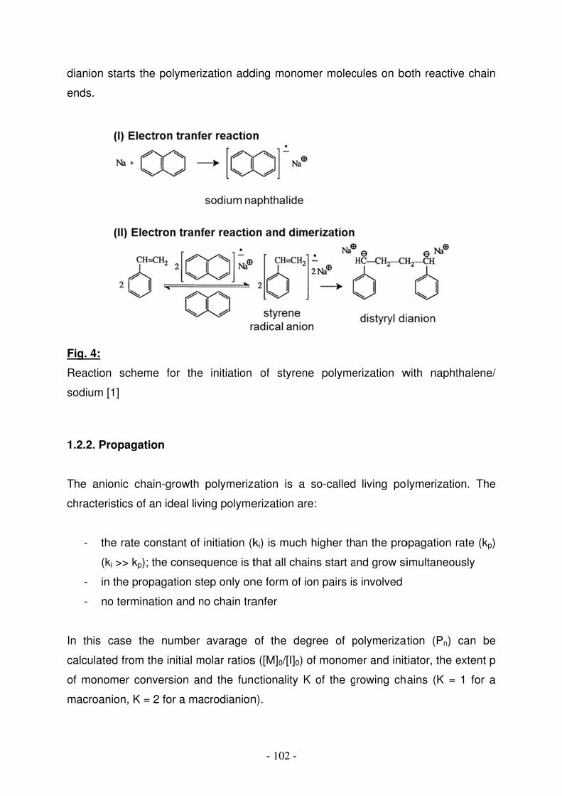
dianion

ends.

Fig. 4:

Reactio

sodium

1.2.2. P

The an

chracte

- t

-

-

In this

calcula

of mon

macroa

n starts the

on schem

m [1]

Propagatio

nionic cha

eristics of a

the rate co

(ki >> kp); t

in the prop

no termina

case the

ated from th

nomer con

anion, K =

e polymeriz

e for the

on

in-growth

an ideal liv

onstant of

the conseq

pagation st

ation and n

e number

he initial m

version an

2 for a ma

zation add

initiation

polymeriz

ing polyme

initiation (k

quence is t

tep only on

no chain tra

avarage

molar ratios

nd the fun

acrodianion

- 102 -

ding monom

of styren

ation is a

erization ar

ki) is much

that all cha

ne form of

anfer

of the de

s ([M]0/[I]0)

ctionality K

n).

mer molec

ne polyme

so-called

re:

h higher th

ains start a

ion pairs is

egree of p

of monom

K of the g

cules on bo

erization w

living po

an the pro

and grow si

s involved

polymerizat

mer and init

rowing ch

oth reactiv

with napht

lymerizatio

opagation r

imultaneou

tion (Pn)

tiator, the e

ains (K =

ve chain

thalene/

on. The

rate (kp)

usly

can be

extent p

1 for a

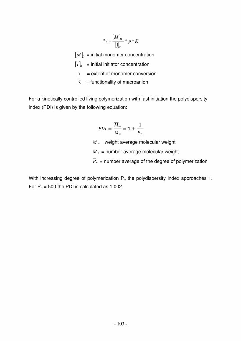
- 103 -

Kp

M**

0IP

0n

0M = initial monomer concentration

0I = initial initiator concentration

p = extent of monomer conversion

K = functionality of macroanion

For a kinetically controlled living polymerization with fast initiation the polydispersity

index (PDI) is given by the following equation:

1 1

wM = weight average molecular weight

nM = number average molecular weight

nP = number average of the degree of polymerization

With increasing degree of polymerization Pn the polydispersity index approaches 1.

For Pn = 500 the PDI is calculated as 1.002.

- 104 -

2. Experimental

2.1. Anionic Polymerization of Styrene/Isoprene

Reagents: toluene from the solvent purification system (SPS)

sec-butyllithium in cyclohexane (1.4 molar)

styrene (freshly distilled)

isoprene (freshly distilled)

methanol (technical grade)

Procedure:

40 ml toluene are added with a syringe through a septum into a completely dry,

argon-flushed 250 ml three necked-flask equipped with a magnetic stir bar. The three

necked-flask is kept under a slight argon stream. The toluene is then heated up to

50°C. Afterwards, 2 ml of styrene are added to the solvent and 0.3 ml of a sec-

butyllithium solution in cyclohexane (1.4 molar) will be injected fast. The reaction

mixture is then stirred for 60 minutes. Subsequently, 6.5 ml of Isoprene are added to

the reaction mixture at room temperature. The solution is stirred again for another 2

hours.

Isolation of the block copolymer

The dissolved polymer is precipitated by dropping the solution under stirring into a

beaker filled with 400 ml of methanol kept at 0°C. Subsequently, the polymer is

filtered by suction filtration, washed with methanol and dried at 50°C in a vacuum

oven.

2.1.2. Evaluation

1) The yield of polymerization is determined.

2) The molar mass averages as well as the molecular weight distribution are

determined by size exclusion chromatography (SEC).

- 105 -

3) Discuss the difference between the theoretically calculated and experimentally

determined values for the molecular weight.

- 106 -

3. Questions

1. How can you calculate the molar mass of the polymer using the monomer and

initiator concentration?

2. How much methanol do you theoretically need to stop the polymerization?

3. Give thereaction equation for the anionic polymerization of styrene with sec-

butyllithium (initiation, propagation and termination reactions).

4. Give the mechanism of the anionic ring opening polymerization of -caprolactam to

synthesize polyamide 6.

107

Versuch 6

Electropolymerization of Conducting Polymers

Assignment of tasks:

1. The theoretical and experimental aspects of the electrochemistry and electropolymerization of

conducting polymers shall be mediated.

2. Voltammetry is introduced as a tool for the synthesis of polythiophene films

3. The electrochromic behavior of the deposited films is studied and correlated to the redox-state.

4. A consistent analysis and evaluation of electrochemical data shall be performed to gain access to

the values of the HOMO level (HOMO = highest occupied molecular orbital)

References:

[1] György Inzelt, Conducting Polymers - A New Era in Electrochemistry, 2nd

Edition, Springer, 2012.

[2] Jürgen Heinze, Bernardo A. Frontana-Uribe, and Sabine Ludwigs, Electrochemistry of Conducting

Polymers - Persistent Models and New Concepts, Chem. Rev., 2010, 110, 4724–4771.

[3] Matthias Rehahn., Elektrisch Leitfähige Kunststoffe, Chemie unserer Zeit 2003, 37, 18-30.

[4] Alan MacDiarmid, Synthetische Metalle: eine neue Rolle für organische Polymere, Angew. Chem.,

2001, 113, 2649-2659.

[5] Jean-Luc Bredas and G.Brian Street, Polarons, bipolarons, and solitons in conducting polymers, Acc.

Chem. Res. 1985, 18, 309–315.

[6] Allen J. Bard and Larry R. Faulkner, Electrochemical Methods – Fundamentals and Applications, John

Wiley & Sons ; 2nd

Edition., 2001.

[7] Carl H. Hamann and Wolf Vielstich, Elektrochemie, Wiley-VCH Verlag GmbH & Co. KGaA, 4th

Edition,

2005.

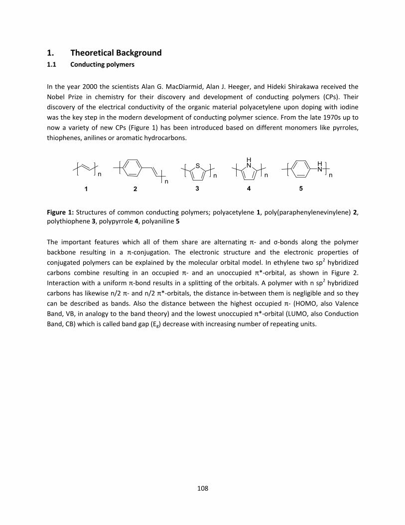
108


1.1 Conducting polymers

In the year 2000 the scientists Alan G. MacDiarmid, Alan J. Heeger, and Hideki Shirakawa received the

Nobel Prize in chemistry for their discovery and development of conducting polymers (CPs). Their

discovery of the electrical conductivity of the organic material polyacetylene upon doping with iodine

was the key step in the modern development of conducting polymer science. From the late 1970s up to

now a variety of new CPs (Figure 1) has been introduced based on different monomers like pyrroles,

thiophenes, anilines or aromatic hydrocarbons.

Figure 1: Structures of common conducting polymers; polyacetylene 1, poly(paraphenylenevinylene) 2,

polythiophene 3, polypyrrole 4, polyaniline 5

The important features hi h all of the share are alter ati g - a d σ-bonds along the polymer

backbone resulting in a -conjugation. The electronic structure and the electronic properties of

conjugated polymers can be explained by the molecular orbital model. In ethylene two sp2 hybridized

carbons combine resulting in an occupied - and an unoccupied *-orbital, as shown in Figure 2.

Interaction with a uniform -bond results in a splitting of the orbitals. A polymer with n sp2 hybridized

carbons has likewise / - a d / *-orbitals, the distance in-between them is negligible and so they

can be described as bands. Also the distance between the highest occupied - (HOMO, also Valence

Band, VB, in analogy to the band theory) and the lowest u o upied *-orbital (LUMO, also Conduction

Band, CB) which is called band gap (Eg) decrease with increasing number of repeating units.

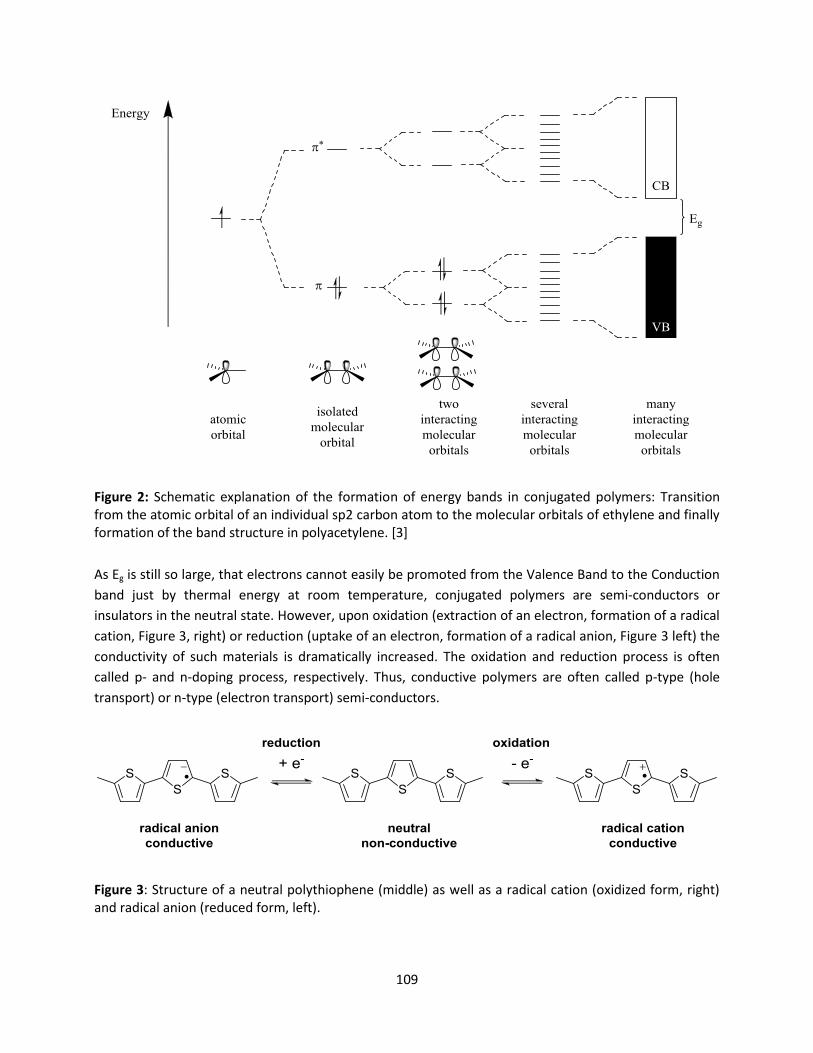
109

Figure 2: Schematic explanation of the formation of energy bands in conjugated polymers: Transition

from the atomic orbital of an individual sp2 carbon atom to the molecular orbitals of ethylene and finally

formation of the band structure in polyacetylene. [3]

As Eg is still so large, that electrons cannot easily be promoted from the Valence Band to the Conduction

band just by thermal energy at room temperature, conjugated polymers are semi-conductors or

insulators in the neutral state. However, upon oxidation (extraction of an electron, formation of a radical

cation, Figure 3, right) or reduction (uptake of an electron, formation of a radical anion, Figure 3 left) the

conductivity of such materials is dramatically increased. The oxidation and reduction process is often

called p- and n-doping process, respectively. Thus, conductive polymers are often called p-type (hole

transport) or n-type (electron transport) semi-conductors.

Figure 3: Structure of a neutral polythiophene (middle) as well as a radical cation (oxidized form, right)

and radical anion (reduced form, left).

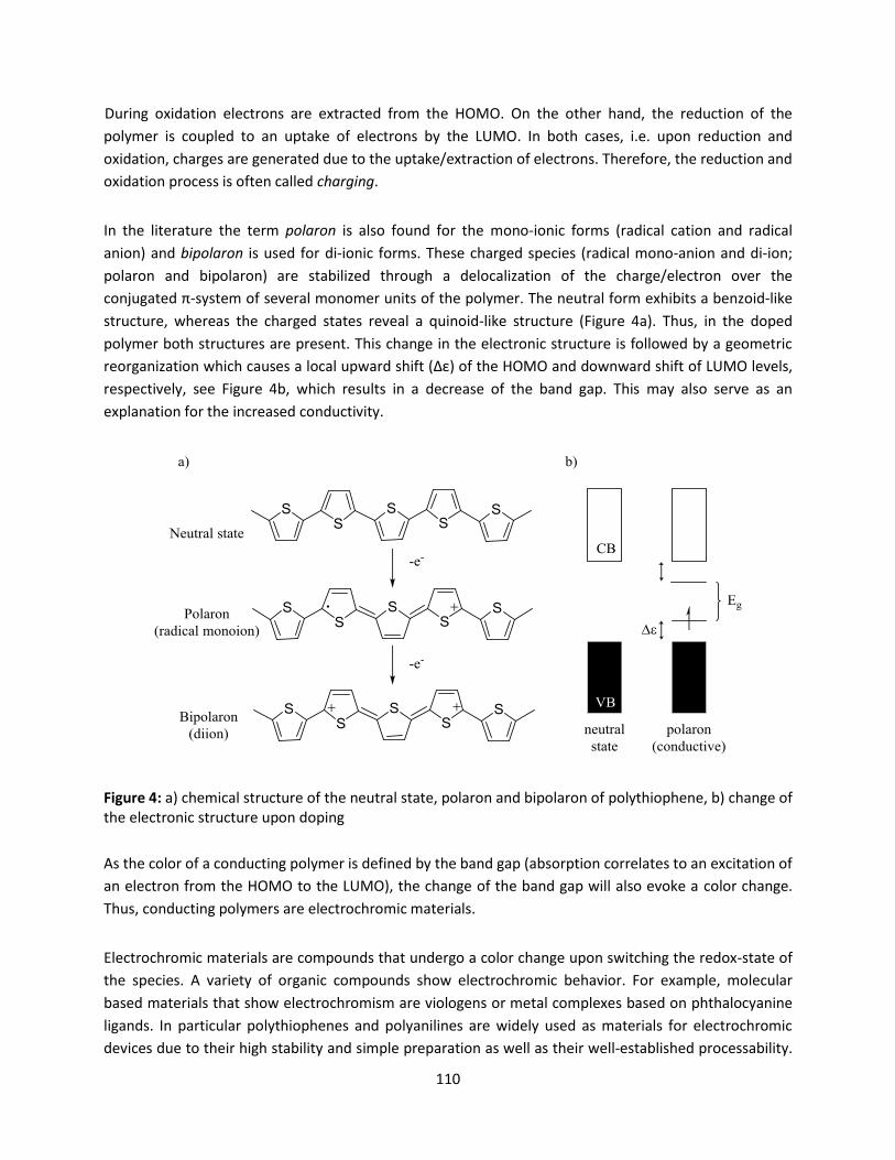
110

During oxidation electrons are extracted from the HOMO. On the other hand, the reduction of the

polymer is coupled to an uptake of electrons by the LUMO. In both cases, i.e. upon reduction and

oxidation, charges are generated due to the uptake/extraction of electrons. Therefore, the reduction and

oxidation process is often called charging.

In the literature the term polaron is also found for the mono-ionic forms (radical cation and radical

anion) and bipolaron is used for di-ionic forms. These charged species (radical mono-anion and di-ion;

polaron and bipolaron) are stabilized through a delocalization of the charge/electron over the

o jugated -system of several monomer units of the polymer. The neutral form exhibits a benzoid-like

structure, whereas the charged states reveal a quinoid-like structure (Figure 4a). Thus, in the doped

polymer both structures are present. This change in the electronic structure is followed by a geometric

reorganization which causes a local upward shift Δε of the HOMO a d downward shift of LUMO levels,

respectively, see Figure 4b, which results in a decrease of the band gap. This may also serve as an

explanation for the increased conductivity.

Figure 4: a) chemical structure of the neutral state, polaron and bipolaron of polythiophene, b) change of

the electronic structure upon doping

As the color of a conducting polymer is defined by the band gap (absorption correlates to an excitation of

an electron from the HOMO to the LUMO), the change of the band gap will also evoke a color change.

Thus, conducting polymers are electrochromic materials.

Electrochromic materials are compounds that undergo a color change upon switching the redox-state of

the species. A variety of organic compounds show electrochromic behavior. For example, molecular

based materials that show electrochromism are viologens or metal complexes based on phthalocyanine

ligands. In particular polythiophenes and polyanilines are widely used as materials for electrochromic

devices due to their high stability and simple preparation as well as their well-established processability.

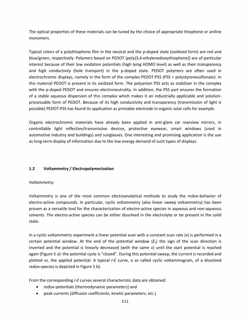
111

The optical properties of these materials can be tuned by the choice of appropriate thiophene or aniline

monomers.

Typical colors of a polythiophene film in the neutral and the p-doped state (oxidized form) are red and

blue/green, respectively. Polymers based on PEDOT (poly(3,4-ethylenedioxythiophene)) are of particular

interest because of their low oxidation potentials (high lying HOMO level) as well as their transparency

and high conductivity (hole transport) in the p-doped state. PEDOT polymers are often used in

electrochromic displays, namely in the form of the complex PEDOT:PSS (PSS = polystyrenesulfonate). In

this material PEDOT is present in its oxidized form. The polyanion PSS acts as stabilizer in the complex

with the p-doped PEDOT and ensures electroneutrality. In addition, the PSS part ensures the formation

of a stable aqueous dispersion of this complex which makes it an industrially applicable and solution-

processable form of PEDOT. Because of its high conductivity and transparency (transmission of light is

possible) PEDOT:PSS has found its application as printable electrode in organic solar cells for example.

Organic electrochromic materials have already been applied in anti-glare car rearview mirrors, in

controllable light reflective/transmissive devices, protective eyewear, smart windows (used in

automotive industry and buildings) and sunglasses. One interesting and promising application is the use

as long-term display of information due to the low energy demand of such types of displays.

1.2 Voltammetry / Electropolymerization

Voltammetry:

Voltammetry is one of the most common electroanalytical methods to study the redox-behavior of

electro-active compounds. In particular, cyclic voltammetry (also linear sweep voltammetry) has been

proven as a versatile tool for the characterization of electro-active species in aqueous and non-aqueous

solvents. The electro-active species can be either dissolved in the electrolyte or be present in the solid

state.

In a cyclic voltammetric experiment a linear potential scan with a constant scan rate (v) is performed in a

certain potential window. At the end of the potential window (Eλ) the sign of the scan direction is

inverted and the potential is linearly decreased (with the same v) until the start potential is reached

again (Figure 5 a : the pote tial le is losed . During this potential sweep, the current is recorded and

plotted vs. the applied potential. A typical I-E curve, a so called cyclic voltammogram, of a dissolved

redox-species is depicted in Figure 5 b).

From the corresponding I-E curves several characteristic data are obtained:

redox-potentials (thermodynamic parameters) and

peak currents (diffusion coefficients, kinetic parameters, etc.)

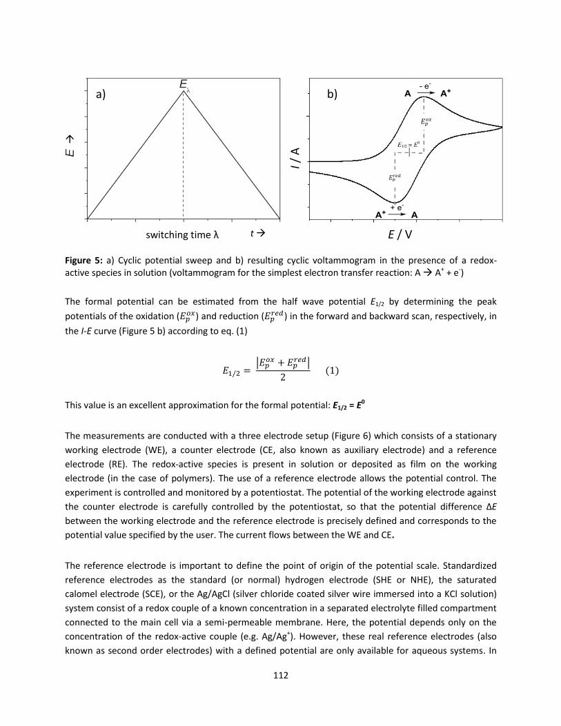
112

Figure 5: a) Cyclic potential sweep and b) resulting cyclic voltammogram in the presence of a redox-

active species in solution (voltammogram for the simplest electron transfer reaction: A A+ + e

-)

The formal potential can be estimated from the half wave potential E1/2 by determining the peak

potentials of the oxidation ( ) and reduction ( ) in the forward and backward scan, respectively, in

the I-E curve (Figure 5 b) according to eq. (1)

| |

This value is an excellent approximation for the formal potential: E1/2 = E0

The measurements are conducted with a three electrode setup (Figure 6) which consists of a stationary

working electrode (WE), a counter electrode (CE, also known as auxiliary electrode) and a reference

electrode (RE). The redox-active species is present in solution or deposited as film on the working

electrode (in the case of polymers). The use of a reference electrode allows the potential control. The

experiment is controlled and monitored by a potentiostat. The potential of the working electrode against

the counter electrode is carefully controlled by the potentiostat, so that the potential differe e ΔE

between the working electrode and the reference electrode is precisely defined and corresponds to the

potential value specified by the user. The current flows between the WE and CE.

The reference electrode is important to define the point of origin of the potential scale. Standardized

reference electrodes as the standard (or normal) hydrogen electrode (SHE or NHE), the saturated

calomel electrode (SCE), or the Ag/AgCl (silver chloride coated silver wire immersed into a KCl solution)

system consist of a redox couple of a known concentration in a separated electrolyte filled compartment

connected to the main cell via a semi-permeable membrane. Here, the potential depends only on the

concentration of the redox-active couple (e.g. Ag/Ag+). However, these real reference electrodes (also

known as second order electrodes) with a defined potential are only available for aqueous systems. In

t

s it hi g ti e λ

a

E / V

I /

A =

E1/2 = E0

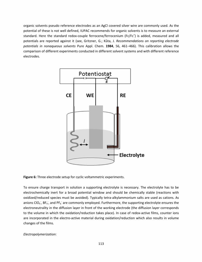
113

organic solvents pseudo reference electrodes as an AgCl covered silver wire are commonly used. As the

potential of these is not well defined, IUPAC recommends for organic solvents is to measure an external

standard. Here the standard redox-couple ferrocene/ferrocenium (Fc/Fc+) is added, measured and all

potentials are reported against it (see, rit er . ta J. Recommendations on reporting electrode

potentials in nonaqueous solvents Pure Appl. Chem. 1984 − . This calibration allows the

comparison of different experiments conducted in different solvent systems and with different reference

electrodes.

Figure 6: Three electrode setup for cyclic voltammetric experiments.

To ensure charge transport in solution a supporting electrolyte is necessary. The electrolyte has to be

electrochemically inert for a broad potential window and should be chemically stable (reactions with

oxidized/reduced species must be avoided). Typically tetra-alkylammonium salts are used as cations. As

anions ClO4-, BF4

-, and PF6

- are commonly employed. Furthermore, the supporting electrolyte ensures the

electroneutrality in the diffusion layer in front of the working electrode (the diffusion layer corresponds

to the volume in which the oxidation/reduction takes place). In case of redox-active films, counter ions

are incorporated in the electro-active material during oxidation/reduction which also results in volume

changes of the films.

Electropolymerization:

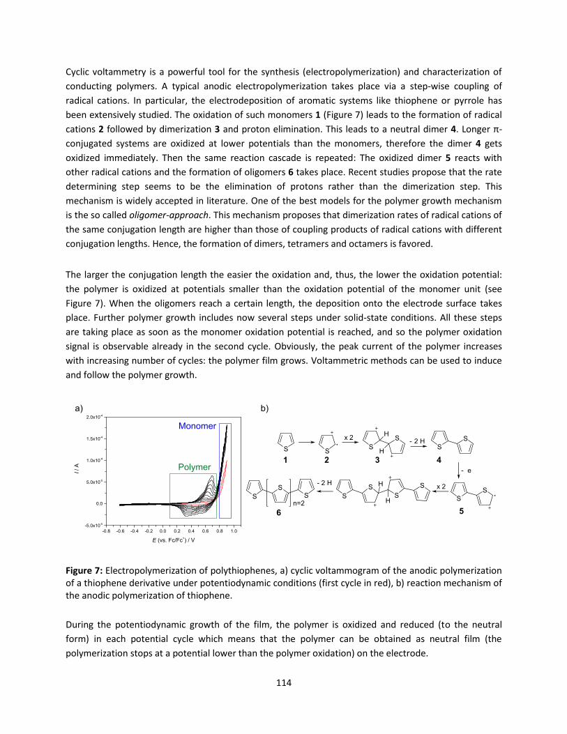
114

Cyclic voltammetry is a powerful tool for the synthesis (electropolymerization) and characterization of

conducting polymers. A typical anodic electropolymerization takes place via a step-wise coupling of

radical cations. In particular, the electrodeposition of aromatic systems like thiophene or pyrrole has

been extensively studied. The oxidation of such monomers 1 (Figure 7) leads to the formation of radical

cations 2 followed by dimerization 3 and proton elimination. This leads to a neutral dimer 4. Lo ger -

conjugated systems are oxidized at lower potentials than the monomers, therefore the dimer 4 gets

oxidized immediately. Then the same reaction cascade is repeated: The oxidized dimer 5 reacts with

other radical cations and the formation of oligomers 6 takes place. Recent studies propose that the rate

determining step seems to be the elimination of protons rather than the dimerization step. This

mechanism is widely accepted in literature. One of the best models for the polymer growth mechanism

is the so called oligomer-approach. This mechanism proposes that dimerization rates of radical cations of

the same conjugation length are higher than those of coupling products of radical cations with different

conjugation lengths. Hence, the formation of dimers, tetramers and octamers is favored.

The larger the conjugation length the easier the oxidation and, thus, the lower the oxidation potential:

the polymer is oxidized at potentials smaller than the oxidation potential of the monomer unit (see

Figure 7). When the oligomers reach a certain length, the deposition onto the electrode surface takes

place. Further polymer growth includes now several steps under solid-state conditions. All these steps

are taking place as soon as the monomer oxidation potential is reached, and so the polymer oxidation

signal is observable already in the second cycle. Obviously, the peak current of the polymer increases

with increasing number of cycles: the polymer film grows. Voltammetric methods can be used to induce

and follow the polymer growth.

Figure 7: Electropolymerization of polythiophenes, a) cyclic voltammogram of the anodic polymerization

of a thiophene derivative under potentiodynamic conditions (first cycle in red), b) reaction mechanism of

the anodic polymerization of thiophene.

During the potentiodynamic growth of the film, the polymer is oxidized and reduced (to the neutral

form) in each potential cycle which means that the polymer can be obtained as neutral film (the

polymerization stops at a potential lower than the polymer oxidation) on the electrode.

115

On the other hand, the electropolymerization can also be performed under potentiostatic control: the

polymerization is conducted at a constant potential for a certain time. This leads ultimately to a polymer

which is in its oxidized/charged state after polymerization. The polymer can be transformed into the

neutral state by applying an appropriate lower potential. Under both electropolymerization conditions

the film thickness can be controlled, by the number of potential cycles under potentiodynamic control

and by the duration of the applied potential under potentiostatic control.

Electrochemical Characterization:

The electrochemical characterization of conducting polymer films deposited on electrodes can be

performed by means of cyclic voltammetric experiments in monomer-free electrolyte. Thus, an influence

of the monomer and further polymer growth can be excluded. Polymers show very broad oxidation and

reduction signals because no longer an one electron process in a small and uniform molecule, but

instead multiple electron processes (polaron, bipolarone) in a non-uniform material (polymerization

degree differe t le gth of effe ti e -conjugation … are o taki g pla e. The resulti g ur e a e described as an overlapping of many redox-events with slightly different redox-potentials, as it is implied

by the grey curves in Figure 8, which could be summed up giving the measured curve (black) of the

oxidation of P3HT (poly(3-hexylthiophene). Hence, the determination of E1/2 is no longer possible and the

onset potential of the oxidation Eox

onset is determined instead by the interception of the two tangents

(blue lines) at the initial slope of the peak. It is assumed that the onset potential value corresponds to

the o idatio /redu tio of the pol er hai s ith the largest o jugated -system.

Figure 8: Typical CV of a polymer film (here, P3HT (poly(3-hexylthiophene), black curve) and potential

depending conductance behaviour (red curve). In grey the overlapping of many different oxidation

waves are schematically shown. The interception of the two tangents (blue lines) at the initial slope of

the peak current corresponds to Eox

onset.

116

From the onset potential values of the oxidation and reduction, the HOMO and LUMO levels,

respectively, of the polymer can be calculated according to equations (2) and (3) (see, C. M. Cardona et

al. Electrochemical Considerations for Determining Absolute Frontier Orbital Energy Levels of Conjugated

Polymers for Solar Cell Applications, Adv. Mater., 2011, 23, 2367–2371)

[ ]

( )[ ]

The value 5.1 corresponds to the formal potential of Fc/Fc+ in the Fermi scale. From the HOMO and

LUMO level, the electrochemical band gap can be estimated according to eq. (4), which is a critical

quantity for polymer based organic photovoltaics.

| |

For P3HT (poly(3-hexylthiophene), a typical electron donor material in organic photovoltaic devices, the

band gap is ≈ 2.3 eV.

117

2. Experiment

Equipment and General Methods:

For all experiments a PGSTAT101 potentiostat from Metrohm and a gas-tight full glass three electrode

cell containing an ITO covered glass slide as working electrode, a Pt plate as counter electrode and a AgCl

covered Ag-wire acting as the reference electrode are used. All manipulations are carried out under

nitrogen atmosphere using standard Schlenk techniques. Solvents are pre-dried and should be handled

under nitrogen atmosphere.

Chemicals:

10 ml of a 0.1 M NBu4PF6/MeCN solution (NBu4PF6: M = 387.43 g/mol),

3,4-ethylenedioxythiophene (EDOT) in a concentration of 0.02 M M = . 8 g/ ol = . g/mL),

CAUTION: EDOT is toxic!

pure acetonitrile, acetone

Electrodeposition:

Two electrochemical cells equipped with a reference electrode are filled with 10 ml of a 0.1 M

NBu4PF6/acetonitrile solution by means of a syringe under nitrogen atmosphere. The electrolyte solution

is deaerated by nitrogen bubbling for approximately 5 min. Then the calculated amount of monomer is

added via a syringe into one of the cells. The working and counter electrode are carefully placed in the

middle of the cell (Note: the working electrode should be placed near the reference electrode to

minimize the effect of an uncompensated IR-drop, an error that is based on the resistance in the

electrolyte solution). EDOT will be electropolymerized by potentiodynamic and potentiostatic control.

- For the potentiodynamic electropolymerization of EDOT, potential cycles in a specified range and scan

rate are performed. The precise values are given by the supervisor and need to be noted for the later

evaluation of the data. The peak maximum in the forward scan of the first cycle corresponds to the

oxidation potential Eox

of the monomer unit. After all cycles have been performed, the polymer covered

electrode is removed and washed gently with pure acetonitrile.

- For the potentiostatic electropolymerization of EDOT a new ITO electrode is mounted in the cell and a

constant potential is applied for a certain time. The polymer covered ITO electrode is removed and

washed gently with pure acetonitrile. The film - which is in its doped state - is stored for further

UV/Vis/NIR spectroscopic characterization. A second PEDOT film is prepared under identical conditions.

This second film is transformed into its neutral state after the deposition by applying a second constant

potential. The precise values are given by the supervisor and need to be noted for the later evaluation of

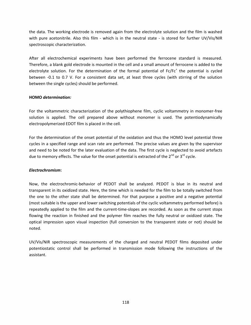
118

the data. The working electrode is removed again from the electrolyte solution and the film is washed

with pure acetonitrile. Also this film - which is in the neutral state - is stored for further UV/Vis/NIR

spectroscopic characterization.

After all electrochemical experiments have been performed the ferrocene standard is measured.

Therefore, a blank gold electrode is mounted in the cell and a small amount of ferrocene is added to the

electrolyte solution. For the determination of the formal potential of Fc/Fc+ the potential is cycled

between -0.1 to 0.7 V. For a consistent data set, at least three cycles (with stirring of the solution

between the single cycles) should be performed.

HOMO determination:

For the voltammetric characterization of the polythiophene film, cyclic voltammetry in monomer-free

solution is applied. The cell prepared above without monomer is used. The potentiodynamically

electropolymerized EDOT film is placed in the cell.

For the determination of the onset potential of the oxidation and thus the HOMO level potential three

cycles in a specified range and scan rate are performed. The precise values are given by the supervisor

and need to be noted for the later evaluation of the data. The first cycle is neglected to avoid artefacts

due to memory effects. The value for the onset potential is extracted of the 2nd

or 3rd

cycle.

Electrochromism:

Now, the electrochromic-behavior of PEDOT shall be analyzed. PEDOT is blue in its neutral and

transparent in its oxidized state. Here, the time which is needed for the film to be totally switched from

the one to the other state shall be determined. For that purpose a positive and a negative potential

(most suitable is the upper and lower switching potentials of the cyclic voltammetry performed before) is

repeatedly applied to the film and the current-time-slopes are recorded. As soon as the current stops

flowing the reaction in finished and the polymer film reaches the fully neutral or oxidized state. The

optical impression upon visual inspection (full conversion to the transparent state or not) should be

noted.

UV/Vis/NIR spectroscopic measurements of the charged and neutral PEDOT films deposited under

potentiostatic control shall be performed in transmission mode following the instructions of the

assistant.

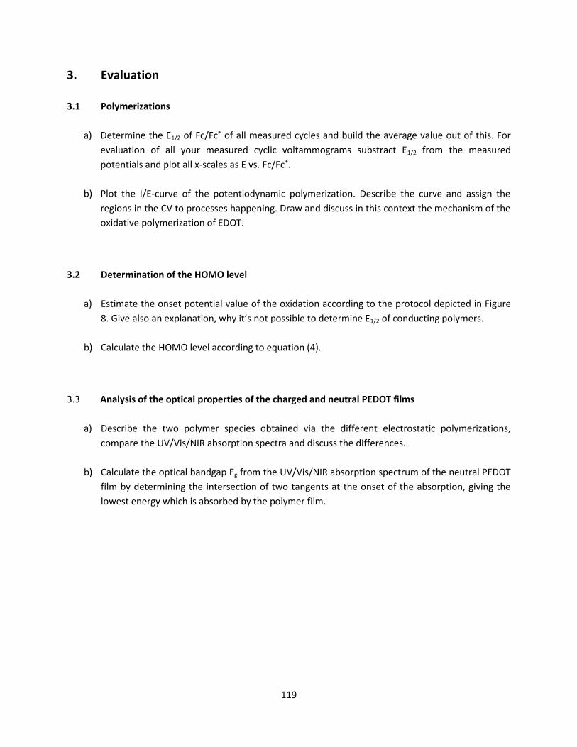
119

3. Evaluation

3.1 Polymerizations

a) Determine the E1/2 of Fc/Fc+ of all measured cycles and build the average value out of this. For

evaluation of all your measured cyclic voltammograms substract E1/2 from the measured

potentials and plot all x-scales as E vs. Fc/Fc+.

b) Plot the I/E-curve of the potentiodynamic polymerization. Describe the curve and assign the

regions in the CV to processes happening. Draw and discuss in this context the mechanism of the

oxidative polymerization of EDOT.

3.2 Determination of the HOMO level

a) Estimate the onset potential value of the oxidation according to the protocol depicted in Figure

8. Give also a e pla atio h it’s ot possi le to deter i e E1/2 of conducting polymers.

b) Calculate the HOMO level according to equation (4).

3.3 Analysis of the optical properties of the charged and neutral PEDOT films

a) Describe the two polymer species obtained via the different electrostatic polymerizations,

compare the UV/Vis/NIR absorption spectra and discuss the differences.

b) Calculate the optical bandgap Eg from the UV/Vis/NIR absorption spectrum of the neutral PEDOT

film by determining the intersection of two tangents at the onset of the absorption, giving the

lowest energy which is absorbed by the polymer film.

120

4. Questions

a) Describe a chemical method for the synthesis of a polythiophene polymer based on a transition

metal complex catalyzed reaction (draw the reaction scheme in which the structure of the

monomer and the resulting polymer shall become clear as well as the catalytic cycle!).

b) Draw the molecular structure of PEDOT:PSS (poly(3,4-ethylenedioxythiophene):

polystyrenesulfonate) in its quinoid stabilized form. In which form is the polystyrenesulfonate

present? Name at least two applications of this conducting polymer.

c) Describe a detailed buildup of an electrochromic window.

d) Name two further electrochemically synthesized polymers and draw their structures.

e) The polymer P3HT is a common donor material in donor-acceptor based organic solar cells. The

acceptor material is often composed of a fullerene derivative (typically PCBM =[6,6]-Phenyl C61

butyric acid methyl ester). Draw a sketch of a polymer based organic solar cell. Draw an energy

diagram containing the HOMO and LUMO levels of the donor and acceptor material.

126

Experiment 10

Viscosimetry

Task

In this experiment the Staudinger index as well as the molar mass of a polystyrene

sample is to be determined by viscosimetry.

Literature

[1] M. Hoffmann, H. Krömer, R. Kuhn, Polymeranalytik, Bd. 1, Thieme Verlag

Stuttgart, 1977.

[2] D. Braun, H. Cherdron, H. Ritter, Praktikum Makromolekularer Stoffe, Wiley-

VCH-Verlag, Weinheim, 1999.

[3] H.-G. Elias, Makromoleküle, Bd. 2, Wiley-VCH-Verlag, 2001.

[4] W.-M. Kulicke, C. Clasen, Viscosimetry of Polymers and Polyelectrolytes,

Springer-Verlag, Berlin, 2004.

[5] B. Tieke, Makromolekulare Chemie, 2. Auflage, Wiley-VCH-Verlag, Weinheim

2005.

[6] Polymer Handbook, 2nd edition, John-Wiley & Sons, New York 1975.

127

Contents

1. Theoretical background

1.1. Determination of molar masses by relative methods

1.2. Viscosimetry

1.3. Viscosity of polymer solutions

1.4. Practical implementation of viscosimetry

2. Experiment

2.1. Procedure

2.2. Evaluation

3. Questions

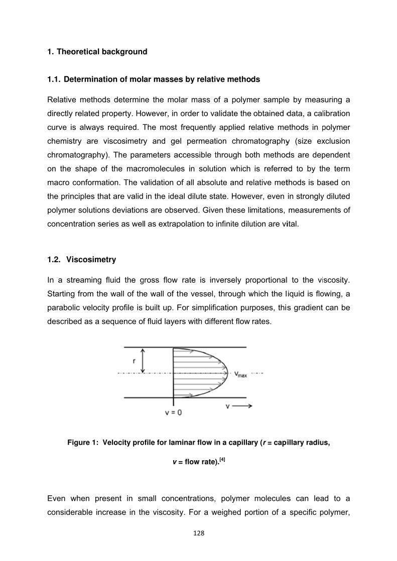
1. Theo

1.1. De

Relativ

directly

curve i

chemis

chroma

on the

macro

the prin

polyme

concen

1.2. V

In a st

Starting

parabo

describ

F

Even w

conside

oretical ba

eterminati

e methods

y related pr

s always

stry are v

atography)

shape of

conformat

nciples tha

er solutions

ntration ser

iscosimet

treaming f

g from the

olic velocity

bed as a se

igure 1: Ve

when pres

erable incr

ackground

on of mol

s determin

roperty. Ho

required. T

iscosimetr

. The para

f the macr

tion. The v

at are valid

s deviation

ries as wel

try

fluid the g

wall of th

y profile is

equence of

elocity pro

sent in sm

rease in th

d

ar masses

ne the mol

owever, in

The most

y and ge

ameters ac

romolecule

validation o

in the idea

ns are obse

l as extrap

gross flow

e wall of th

built up. F

f fluid laye

ofile for lam

v =

mall conce

he viscosity

128

s by relati

lar mass o

order to va

frequently

el permeat

ccessible t

es in solut

of all absol

al dilute st

erved. Give

polation to

rate is in

he vessel,

For simplifi

rs with diff

minar flow i

= flow rate)

entrations,

y. For a w

ive metho

of a polym

alidate the

y applied r

tion chrom

through bo

tion which

lute and re

tate. Howe

en these li

infinite dilu

versely pr

through w

ication pur

ferent flow

in a capilla

).[4]

polymer

weighed po

ds

mer sample

obtained d

elative me

matography

oth method

is referre

elative met

ver, even

mitations,

ution are vi

roportional

which the l

rposes, this

rates.

ry (r = capi

molecules

ortion of a

e by meas

data, a cal

ethods in p

y (size ex

ds are dep

ed to by th

thods is ba

in strongly

measurem

ital.

l to the vi

iquid is flo

s gradient

illary radiu

s can lea

specific p

suring a

libration

polymer

xclusion

pendent

he term

ased on

y diluted

ments of

scosity.

owing, a

can be

us,

ad to a

polymer,

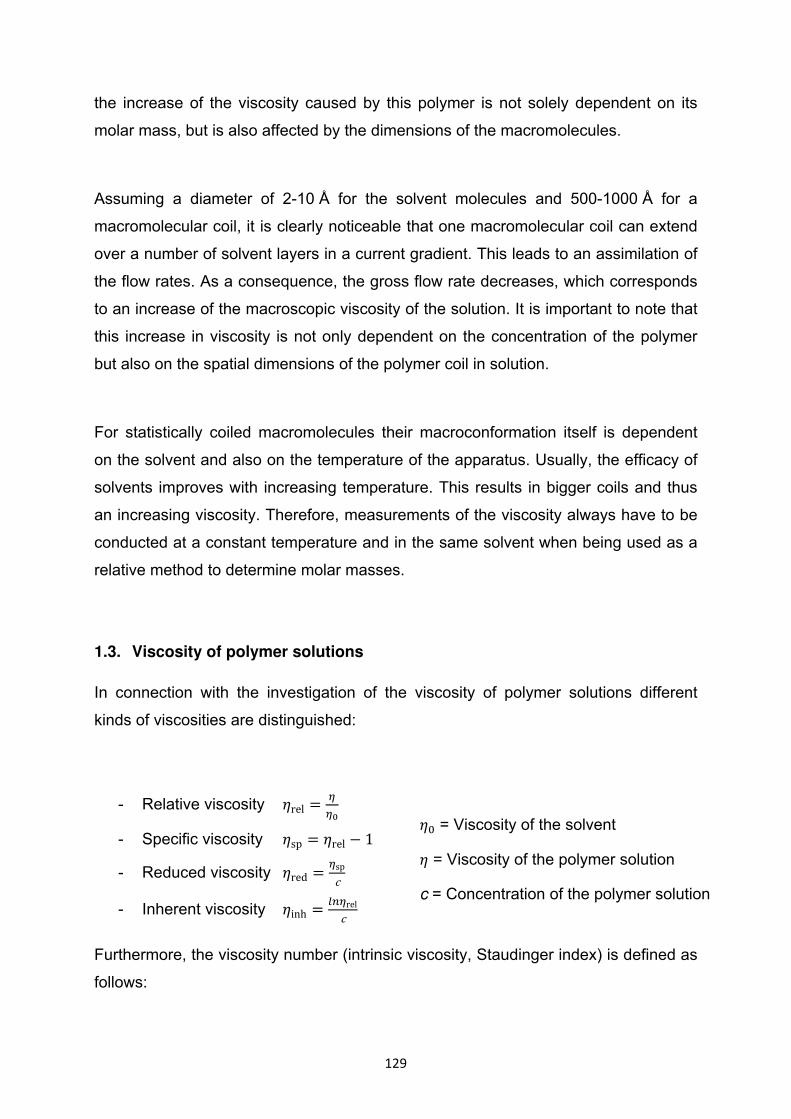
129

the increase of the viscosity caused by this polymer is not solely dependent on its

molar mass, but is also affected by the dimensions of the macromolecules.

Assuming a diameter of 2-10 Å for the solvent molecules and 500-1000 Å for a

macromolecular coil, it is clearly noticeable that one macromolecular coil can extend

over a number of solvent layers in a current gradient. This leads to an assimilation of

the flow rates. As a consequence, the gross flow rate decreases, which corresponds

to an increase of the macroscopic viscosity of the solution. It is important to note that

this increase in viscosity is not only dependent on the concentration of the polymer

but also on the spatial dimensions of the polymer coil in solution.

For statistically coiled macromolecules their macroconformation itself is dependent

on the solvent and also on the temperature of the apparatus. Usually, the efficacy of

solvents improves with increasing temperature. This results in bigger coils and thus

an increasing viscosity. Therefore, measurements of the viscosity always have to be

conducted at a constant temperature and in the same solvent when being used as a

relative method to determine molar masses.

1.3. Viscosity of polymer solutions

In connection with the investigation of the viscosity of polymer solutions different

kinds of viscosities are distinguished:

- Relative viscosity rel

- Specific viscosity sp rel 1

- Reduced viscosity red spc

- Inherent viscosity inh relc

Furthermore, the viscosity number (intrinsic viscosity, Staudinger index) is defined as

follows:

= Viscosity of the solvent

= Viscosity of the polymer solution

c = Concentration of the polymer solution

η rep

shear r

plottingηspc vers

temper

Fi

In mos

shear r

growing

neglect

the flow

1.4. P

resents the

rate of G

g ηspc versus

sus c for

rature of 25

gure 2: Re

molec

st cases it

rate. Even

g molecul

t this effec

wing mater

ractical im

e limit of th

= 0. It is p

s c. This of

polystyren

5 C.

duced visc

cular weigh

is forborne

though sta

ar weight

ct when vis

rial are use

mplementa

ηhe quotien

possible to

ften leads t

ne sample

cosities as

hts of polys

e to condu

atistical co

under the

scometers

ed.

ation of vi

130

limc→G→

nt ηspc at a c

o perform

to a linear

es exhibiti

a function

styrene (me

uct an extr

oils of poly

e influence

showing o

scosimetr

concentrati

a graphica

correlation

ing differe

n of the con

easured in

rapolation

mers tend

e of shea

only a sma

ry

on of c = 0

al extrapo

n. Figure 2

nt molecu

ncentration

toluene at

to c = 0 w

to increas

ar, it is us

all gradient

0 and in ca

olation to c

2 shows the

ular weigh

n for differe

t 25 C).

with respec

singly defo

sually pos

t in the ve

(1)

ase of a

c = 0 by

e plot of

ts at a

ent

ct to the

orm with

sible to

locity of

Measu

Ostwal

shows

Fig

Hagen-

determ

rements a

d- and the

a schemat

gure 3: Sch

-Poiseuille

ination of t

are perform

e Ubbelohd

tic illustrati

heme of an

’s law pro

the viscosi

r = capil

t = flow Δ = pre

l = capil

V = cap

= dens

h = heig

med in so-

de-viscome

ion of both

n Ostwald-

vides the

ity η of a p

llary radius

time

essure diffe

lary length

illary volum

sity of the

ght

131

-called cap

eter belong

h types of v

(left) and a

theoretica

olymer sol

∙ ∙with Δ

s

erence at t

h

me

solution

pillary visc

g to the mo

viscometer

an Ubbeloh

al basis for

lution:

∙ ∙∙

∙ g ∙ h.

the capillar

cometers, a

ost frequen

s.

hde-viscom

r the meas

ry

among wh

ntly used. F

meter (right

surement a

hich the

Figure 3

t).[5]

and the

(2)

132

The measurement itself is based on determining the time that a polymer solution

takes to travel a distinct distance in the capillary of the viscometer.

Considering Hagen-Poisseuille’s law the specific viscosity sp can be expressed in

the following way:

sp . (3)

As for small concentrations the density of the solution and the density of the

solvent are approximately the same, one can simplify (3) as follows:

sp . (4)

For linear, statistically coiled polymers the Staudinger index is linked to the molecular

weight via the Mark-Houwink equation, where represents the viscosity average

molar mass.

η K∙Mηa . (5)

The variables K and a are dependent on the geometrical form of the dissolved

polymer coil as well as on the type of solvent and the temperature. The value of a in

particular reflects the conformation of the polymer and is closely related to the

second virial coefficient. Usually the parameter a adopts values in the range between

0.6 and 0.9. In θ-solvents and at the corresponding θ-temperature a has a value of

0.5. In case of a non-perfused coil one obtains a = 0 and for a rigid rod a = 2. For

polymers with a known molar mass it is possible to extract the a and K values from a

double logarithmic plot of η versus resulting in a straight line where a and K are

represented by the slope and the y-intercept, respectively. Specific values for the

parameters a and K are documented in the literature for a variety of polymer-solvent-

temperature-systems.

In addition, the Staudinger index of a polydisperse substance without any interactions

can be expressed as an average weight (Philippoff-equation):

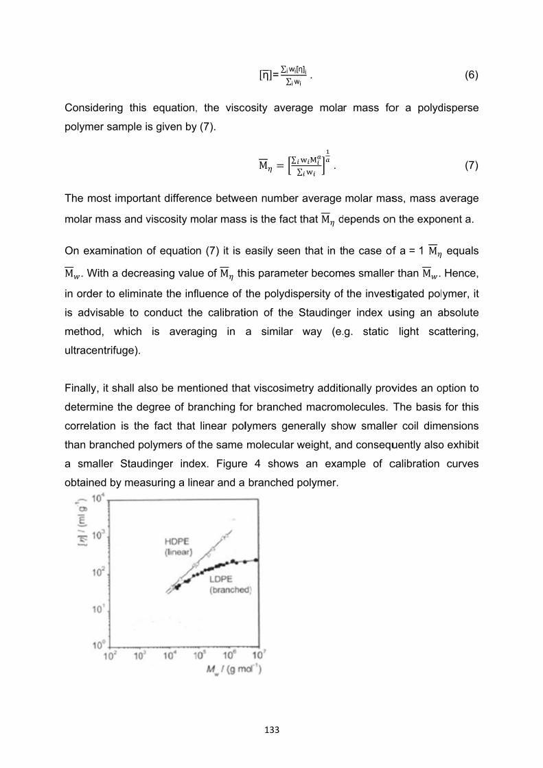
Consid

polyme

The mo

molar m

On exaM . Wi

in orde

is advi

method

ultrace

Finally,

determ

correla

than br

a sma

obtaine

ering this

er sample i

ost importa

mass and v

amination o

ith a decre

er to elimin

sable to c

d, which

ntrifuge).

, it shall als

ine the de

tion is the

ranched po

ller Staud

ed by meas

equation,

s given by

ant differen

viscosity m

of equatio

easing valu

ate the inf

conduct th

is avera

so be men

egree of br

e fact that

olymers of

dinger inde

suring a lin

, the visco

y (7).

nce betwe

molar mass

n (7) it is e

ue of M th

fluence of t

e calibrati

ging in

ntioned tha

ranching fo

linear pol

the same

ex. Figure

near and a

133

η =∑ wi∑ wi

osity aver

M ∑en numbe

s is the fact

easily see

his parame

the polydis

ion of the

a similar

at viscosim

or branche

lymers ge

molecular

e 4 shows

branched

i[η]iwi

.

rage mola

∑∑ .

r average

t that M d

n that in t

eter becom

spersity of

Staudinge

way (e.

metry additi

ed macrom

nerally sho

weight, an

s an exam

polymer.

r mass fo

molar mas

epends on

he case of

es smaller

the invest

er index u

g. static

onally prov

molecules.

ow smalle

nd consequ

mple of c

or a polyd

ss, mass a

n the expon

f a = 1 Mr than M .

tigated pol

using an a

light sca

vides an o

The basis

er coil dim

uently also

calibration

(6)

disperse

(7)

average

nent a.

equals

Hence,

ymer, it

absolute

attering,

option to

for this

ensions

o exhibit

curves

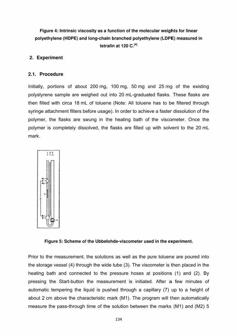
Fi

poly

2. Ex

2.1. P

Initially

polysty

then fil

syringe

polyme

polyme

mark.

Prior to

the sto

heating

pressin

automa

about 2

measu

igure 4: Int

yethylene (

periment

rocedure

, portions

yrene samp

led with c

e attachme

er, the flas

er is comp

Figure 5:

o the meas

rage vesse

g bath and

ng the Sta

atic tempe

2 cm abov

re the pas

trinsic visc

(HDPE) and

s of about

ple are we

circa 18 mL

ent filters be

sks are sw

pletely diss

Scheme of

surement,

el (4) throu

d connect

art-button

ring the li

ve the char

ss-through

cosity as a

d long-chai

tetra

t 200 mg,

eighed out

L of toluen

efore usag

wung in t

solved, the

f the Ubbel

the solutio

ugh the wid

ted to the

the meas

quid is pu

racteristic

time of th

134

function o

in branche

ralin at 120

, 100 mg,

t into 20 m

ne (Note: A

ge). In orde

he heating

e flasks ar

lohde-visco

ons as we

de tube (3)

pressure

surement

ushed thro

mark (M1)

he solution

of the molec

ed polyethy

C.[4]

50 mg a

mL-graduat

All toluene

er to achiev

g bath of

re filled up

ometer use

ll as the p

). The visc

hoses at

is initiated

ugh a cap

). The prog

between

cular weigh

ylene (LDPE

and 25 mg

ed flasks.

e has to b

ve a faster

the visco

p with solv

ed in the ex

ure toluen

ometer is t

t positions

d. After a

pillary (7)

gram will t

the marks

hts for line

E) measure

g of the

These fla

be filtered

r dissolutio

ometer. On

vent to the

xperiment.

ne are pou

then place

s (1) and

a few min

up to a he

then autom

s (M1) and

ear

ed in

existing

sks are

through

on of the

nce the

e 20 mL

red into

ed in the

(2). By

utes of

eight of

matically

(M2) 5

135

times in succession. If these 5 measurements do not lead to reproducible results,

another set of 5 measurements should be performed. Important: Every time you start

a new set of measurements, all values of the previous measurement are deleted.

Therefore, it is crucial to copy the results manually. Between the measurements the

viscometers are thoroughly rinsed with toluene (3x) and acetone (2x) and

subsequently dried with compressed air.

2.2. Evaluation

All measured values are summarized in one table. The values that are important for

the following calculations are the corrected average values. According to equation

(4) sp is determined. The values thus obtained are then used to calculate sp by

dividing sp by the respective concentrations. Plotting sp versus c (g/mL) and

extrapolation to c = 0 gives the Staudinger index η , from which the molar mass of

the polystyrene sample can be calculated according to equation (5).

K- and a-values for polystyrene in toluene at 30 °C: K = 0.012 mL/g, a = 0.71.[6]

3. Questions

1) How and why do the Staudinger indices of polystyrene, polystyrene-lithium

and sulfonated polystyrene differ?

2) Which factors for the determination of the Staudinger index are no longer

negligible at concentrations below 2 · 10-2 g/mL?

3) What is the difference between Ostwald- and Ubbelohde-viscometers?

4) Which solution exhibits the bigger Staudinger index – it-PMMA/3-heptanone or

at-PMMA/3-heptanone? (same molecular weights and measuring conditions)

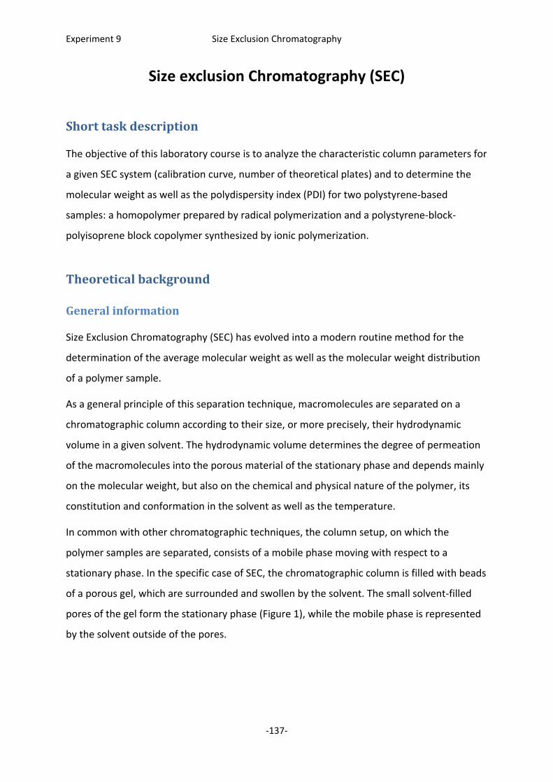
Experiment 9 Size Exclusion Chromatography

‐137‐

Size exclusion Chromatography (SEC)

Shorttaskdescription

The objective of this laboratory course is to analyze the characteristic column parameters for

a given SEC system (calibration curve, number of theoretical plates) and to determine the

molecular weight as well as the polydispersity index (PDI) for two polystyrene‐based

samples: a homopolymer prepared by radical polymerization and a polystyrene‐block‐

polyisoprene block copolymer synthesized by ionic polymerization.

Theoreticalbackground

Generalinformation

Size Exclusion Chromatography (SEC) has evolved into a modern routine method for the

determination of the average molecular weight as well as the molecular weight distribution

of a polymer sample.

As a general principle of this separation technique, macromolecules are separated on a

chromatographic column according to their size, or more precisely, their hydrodynamic

volume in a given solvent. The hydrodynamic volume determines the degree of permeation

of the macromolecules into the porous material of the stationary phase and depends mainly

on the molecular weight, but also on the chemical and physical nature of the polymer, its

constitution and conformation in the solvent as well as the temperature.

In common with other chromatographic techniques, the column setup, on which the

polymer samples are separated, consists of a mobile phase moving with respect to a

stationary phase. In the specific case of SEC, the chromatographic column is filled with beads

of a porous gel, which are surrounded and swollen by the solvent. The small solvent‐filled

pores of the gel form the stationary phase (Figure 1), while the mobile phase is represented

by the solvent outside of the pores.

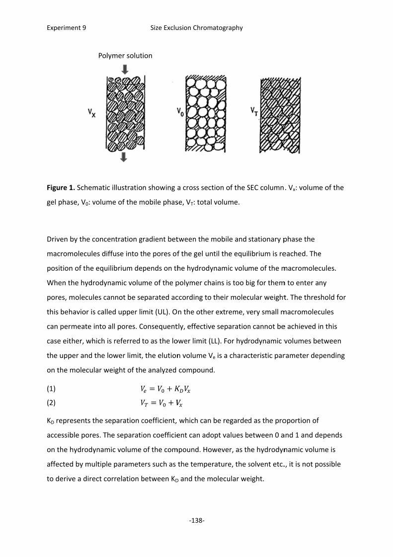
Experim

Figure 1

gel phas

Driven b

macrom

position

When t

pores, m

this beh

can per

case eit

the upp

on the m

(1)

(2)

KD repre

accessib

on the h

affected

to deriv

ent 9

1. Schemati

se, V0: volum

by the conc

molecules di

n of the equ

he hydrody

molecules c

havior is cal

meate into

ther, which

per and the

molecular w

esents the s

ble pores. T

hydrodynam

d by multipl

ve a direct c

Po

c illustratio

me of the m

centration g

iffuse into t

uilibrium de

ynamic volu

annot be se

led upper li

all pores. C

is referred

lower limit,

weight of th

separation c

The separati

mic volume

le paramete

correlation b

lymer solut

Size Exclu

n showing a

mobile phas

gradient bet

the pores of

pends on th

me of the p

eparated ac

mit (UL). O

Consequent

to as the lo

, the elution

e analyzed

coefficient,

ion coefficie

of the com

ers such as

between KD

ion

usion Chrom

‐138‐

a cross sect

se, VT: total

tween the m

f the gel un

he hydrody

polymer cha

ccording to

n the other

tly, effective

ower limit (L

n volume Ve

compound

which can

ent can ado

mpound. How

the temper

D and the m

atography

tion of the S

volume.

mobile and

til the equi

ynamic volu

ains is too b

their molec

r extreme, v

e separation

LL). For hydr

e is a charac

.

be regarded

opt values b

wever, as th

rature, the s

olecular we

SEC column

stationary p

librium is re

me of the m

big for them

cular weight

very small m

n cannot be

rodynamic v

cteristic par

d as the pro

etween 0 a

he hydrodyn

solvent etc.

eight.

. Vx: volume

phase the

eached. The

macromolec

m to enter an

t. The thres

macromolec

e achieved i

volumes be

rameter dep

oportion of

and 1 and de

namic volum

., it is not po

e of the

e

cules.

ny

shold for

cules

n this

etween

pending

epends

me is

ossible

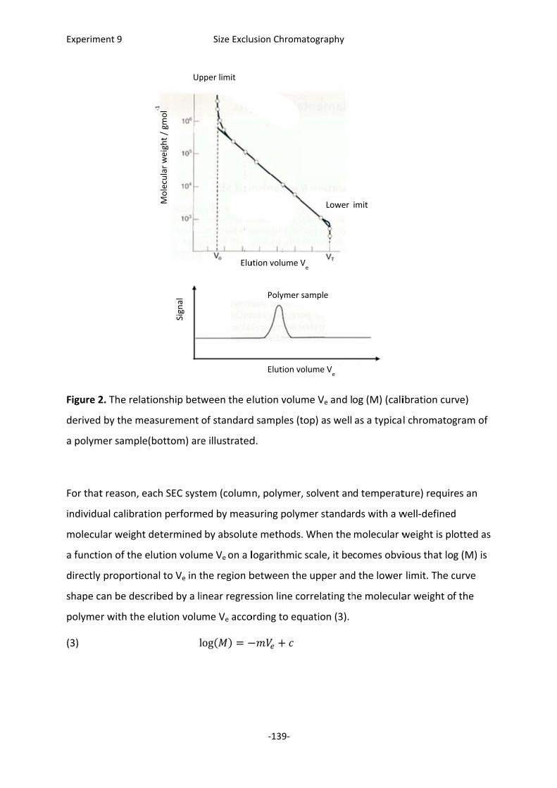
Experim

Figure 2

derived

a polym

For that

individu

molecu

a functi

directly

shape c

polyme

(3)

ent 9

2. The relati

by the mea

mer sample(

t reason, ea

ual calibratio

lar weight d

on of the e

proportion

an be descr

r with the e

ionship betw

asurement

bottom) are

ach SEC syst

on perform

determined

lution volum

nal to Ve in t

ribed by a li

elution volul

Up

Molecular w

eight /

gmol‐1

Signal

Size Exclu

ween the e

of standard

e illustrated

tem (colum

ed by meas

by absolut

me Ve on a l

the region b

inear regres

me Ve accolog

pper limit

Elu

usion Chrom

‐139‐

lution volum

d samples (t

d.

n, polymer,

suring polym

e methods.

logarithmic

between the

ssion line co

ording to eq

ution volume V

Elution vo

Polymer s

atography

me Ve and l

top) as well

, solvent an

mer standar

. When the

scale, it be

e upper and

orrelating th

uation (3).

Lower l

Ve

olume Ve

sample

og (M) (cali

as a typica

d temperat

rds with a w

molecular w

comes obvi

d the lower

he molecula

imit

ibration cur

l chromatog

ture) requir

well‐defined

weight is pl

ious that lo

r limit. The c

ar weight o

rve)

gram of

res an

d

otted as

g (M) is

curve

f the

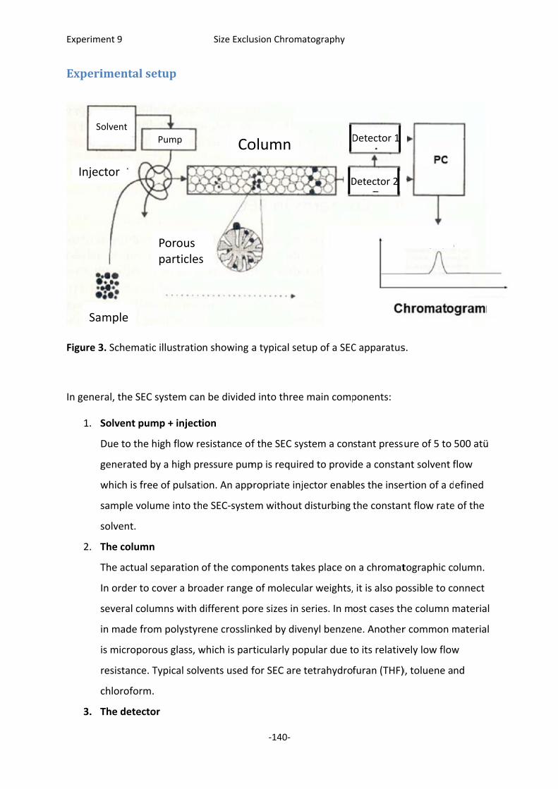
Experim

Experi

Figure 3

In gene

1. S

g

w

s

s

2. T

T

s

c

3. T

S

Injec

Sa

ent 9

imentals

3. Schemati

ral, the SEC

Solvent pum

Due to the

generated b

which is fre

sample volu

solvent.

The column

The actual s

In order to

several colu

in made fro

is micropor

resistance.

chloroform

The detecto

olvent

ctor

mple

etup

c illustratio

C system can

mp + inject

high flow re

by a high pr

ee of pulsati

ume into th

n

separation

cover a bro

umns with d

om polystyr

rous glass, w

Typical solv

.

or

Pump

Porous particles

Size Exclu

n showing a

n be divided

ion

esistance of

ressure pum

ion. An app

he SEC‐syste

of the comp

oader range

different po

ene crosslin

which is par

vents used f

Co

s

usion Chrom

‐140‐

a typical set

d into three

f the SEC sy

mp is requir

propriate inj

em without

ponents tak

e of molecul

ore sizes in s

nked by dive

rticularly po

for SEC are

olumn

atography

tup of a SEC

e main comp

ystem a con

ed to provid

jector enab

disturbing

kes place on

lar weights,

series. In m

enyl benzen

opular due t

tetrahydro

D

D

C apparatus

ponents:

stant press

de a consta

les the inse

the constan

n a chromat

it is also po

ost cases th

ne. Another

o its relativ

furan (THF)

Detector 1

Detector 2

s.

ure of 5 to

ant solvent f

ertion of a d

nt flow rate

tographic co

ossible to co

he column m

r common m

vely low flow

), toluene a

500 atü

flow

efined

e of the

olumn.

onnect

material

material

w

nd

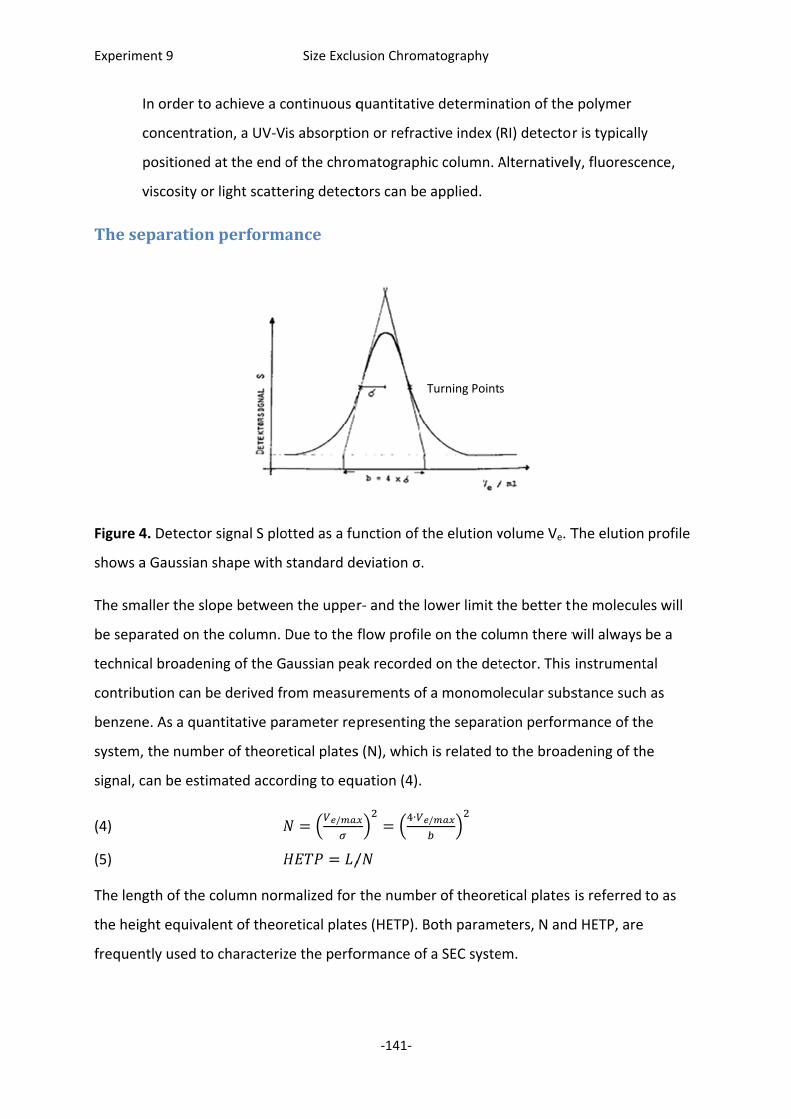
Experim

c

v

These

Figure 4

shows a

The sma

be sepa

technica

contribu

benzene

system,

signal, c

(4)

(5)

The leng

the heig

frequen

ent 9

In order to

concentrati

positioned

viscosity or

eparation

4. Detector

a Gaussian s

aller the slo

arated on th

al broadeni

ution can be

e. As a quan

, the numbe

can be estim

gth of the c

ght equivale

ntly used to

achieve a c

ion, a UV‐V

at the end o

light scatte

performa

signal S plo

shape with

ope betwee

he column. D

ng of the G

e derived fr

ntitative pa

er of theore

mated accor

column norm

ent of theor

characteriz

Size Exclu

ontinuous q

is absorptio

of the chrom

ering detect

ance

otted as a fu

standard de

n the upper

Due to the f

aussian pea

rom measur

rameter rep

etical plates

rding to equ

/ /malized for

retical plate

ze the perfo

usion Chrom

‐141‐

quantitative

on or refrac

matograph

tors can be

unction of th

eviation σ.

r‐ and the lo

flow profile

ak recorded

rements of

presenting

s (N), which

uation (4).

∙/

the numbe

es (HETP). B

ormance of

T

atography

e determina

tive index (

ic column. A

applied.

he elution v

ower limit t

e on the col

d on the det

a monomo

the separat

is related t

/

er of theore

Both parame

a SEC syste

Turning Points

ation of the

RI) detecto

Alternativel

volume Ve. T

the better th

umn there w

tector. This

lecular subs

tion perform

o the broad

tical plates

eters, N and

em.

s

e polymer

r is typically

ly, fluoresce

The elution

he molecul

will always

instrument

stance such

mance of th

dening of th

is referred

d HETP, are

y

ence,

profile

es will

be a

tal

h as

he

he

to as


‐142‐

Dataanalysis

Synthetic polymers usually comprise a mixture of molecular weights. Therefore, the

characteristic elution profile of a polymer sample represents the sum of all components.

Even though the separation of all the different molecular weight fractions into completely

distinct signals proofs to be impossible in many cases, the shape of the elution curve

provides information about the molecular weight distribution of the polymer.

From the distribution profile of the molecular weight, the number‐averaged molecular

weight Mn as well as the weight‐averaged molecular weight Mw can be derived as

characteristic parameters for the description of a polymer sample. These properties are

defined as follows:

(6) ∑∑ ∑∑ ∑∑

(7) ∑∑ ∑∑ ∑∑

To each value of Ve in the elusion diagram a molecular weight Mi can be assigned, while the

abundance of molecule i is related to the detector intensity Hi.

Experimentaldetails

The aim of this practical course is to use the SEC method to determine the average

molecular weight values Mn and Mw as well as the molecular weight distribution for two

polymer samples, the first of which being a polystyrene homopolymer synthesized by radical

polymerization (sample from experiment 2), while the second one represents a polystyrene‐

block‐polyisoprene copolymer prepared by ionic polymerization (sample from experiment 7).

The calibration curve for the specific SEC system used in the experiments will be provided by

the demonstrator.

Prior to the analysis, the polymer samples have to be dissolved in THF (approximately 5%

w/w) followed by filtering through a syringe filter with 450 µm pore diameter. Subsequently,

the samples are applied onto the SEC system to record the chromatogram. The number of

theoretical plates and the HETP value should be determined by the evaluation of the o‐

dichlorobenzene signal.


‐143‐

Requirementsfordataanalysisandreport

Introduction including the theoretical background of the method and a description of the experimental setup.

Comparison of the different elution curves and detailed description of all signals. Analysis of the molecular weight distribution and averaged molecular weights Detailed discussion and comparison of the results.

Questions

1. How is the column volume defined?

2. Which absolute methods for the measurement of the molecular weight do you know

and how can you determine the molecular weight distribution?

3. How can continuous degassing of the solvent be achieved?

4. Which parameters influence the separation performance of the SEC‐system?

5. Which requirements do the pump and detectors have to fulfill?

6. Explain the setup of a differential refractometer!

144

Experiment 9

Thermal Analysis of Polymers by Means of Differential Scanning Calorimetry (DSC)

Task

Different thermal phase transitions of amorphous and semi-crystalline polymers

should be investigated by means of DSC.

Literature

1) H.-G. Elias, Makromoleküle, Bd. 2: Physikalische Strukturen und Eigenschaften, Wiley-VCH

Weinheim, 2001

2) W.F. Hemminger, H.K. Cammenga, Methoden der thermischen Analyse, Springer-Verlag, Berlin

1989

3) G.W.H. Höhne, W.F. Hemminger, H.-J. Flammersheim, Differential Scanning Calorimetry, Springer-

Verlag, Berlin 2003

Content


1.1 Polymers in the Solid State

1.2 Thermal Phase Transitions

1.3 Analysis of Thermal Phase Transitions

1.3.1 Measuring Principle of DSC

1.3.2 Thermal Phase Transitions - Examples and Interpretation

2. Experimental Section

3. Evaluation

4. Questions

145


1.1 Polymers in the Solid State

a) Amorphous Polymers

In the melt state, polymers exist as random coils (undisturbed dimensions, -state),

which interpenetrate each other. If the polymer exhibits a sufficiently high molecular

weight, this effect leads to a rubber-elastic melt, where the elasticity is based on

entanglements between the chains.

Upon temperature reduction, the viscosity of the melt increases strongly until a glassy

solidification occurs. The glass shows a similar microstructure as the melt and the

characteristic transition temperature is referred to as the glass temperature Tg. At the

molecular level the mobility of the chains becomes strongly reduced during the

transition from melt to glass. Further cooling leads to a reduced mobility of the main

chains and thus the material becomes brittle.

The formation of a glass, which does not have a possibility for crystallization, requires

an irregular structure of the polymer chains. A frequently used approach to obtain

amorphous structures of polymers that are otherwise capable of crystallization, is the

disturbance of the crystallization process by the introduction of comonomers or by

rapid quenching from melt.

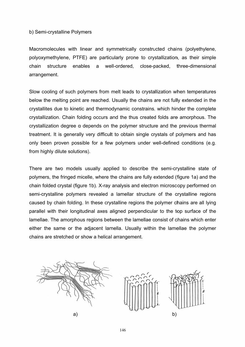
b) Sem

Macrom

polyoxy

chain

arrange

Slow c

below t

crystall

crystall

crystall

treatme

only be

from hi

There

polyme

chain fo

semi-cr

caused

paralle

lamella

either t

chains

mi-crystallin

molecules

ymethylene

structure

ement.

ooling of s

the melting

ites due to

ization. Ch

ization deg

ent. It is g

een prove

ghly dilute

are two m

ers, the frin

olded crys

rystalline p

d by chain

l with thei

ae. The am

the same

are stretch

ne Polymer

with linea

e, PTFE)

enables

such polym

g point are

o kinetic a

hain foldin

gree α dep

enerally ve

n possible

solutions)

models us

nged micel

tal (figure

polymers

folding. In

r longitudi

morphous re

or the ad

hed or sho

a)

rs

ar and sy

are partic

s a we

mers from

e reached.

nd thermo

g occurs a

pends on

ery difficul

e for a few

).

sually app

le, where t

1b). X-ray

revealed

n these cry

nal axes a

egions bet

djacent lam

w a helica

146

ymmetrical

cularly pro

ell-ordered

melt leads

Usually th

odynamic c

and the th

the polym

lt to obtain

w polymer

plied to de

the chains

analysis a

a lamellar

ystalline re

aligned pe

tween the

mella. Usu

l arrangem

ly constru

one to crys

, close-p

s to crysta

he chains a

constrains,

us created

er structur

n single cr

rs under w

escribe th

are fully e

and electro

r structure

gions the

erpendicula

lamellae c

ually within

ment.

ucted chain

stallization

packed, t

llization wh

are not full

which hin

d folds are

re and the

ystals of p

well-defined

e semi-cr

extended (f

on microsco

e of the c

polymer ch

ar to the to

onsist of c

n the lame

b)

ns (polyet

n, as their

three-dime

hen tempe

ly extende

nder the co

e amorpho

previous

polymers a

d condition

rystalline s

figure 1a)

copy perfor

crystalline

hains are

op surface

chains whic

ellae the p

thylene,

simple

ensional

eratures

d in the

omplete

us. The

thermal

and has

ns (e.g.

state of

and the

rmed on

regions

all lying

e of the

ch enter

polymer

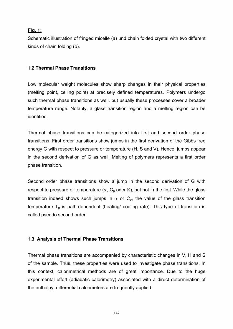
147

Fig. 1:

Schematic illustration of fringed micelle (a) und chain folded crystal with two different

kinds of chain folding (b).

1.2 Thermal Phase Transitions

Low molecular weight molecules show sharp changes in their physical properties

(melting point, ceiling point) at precisely defined temperatures. Polymers undergo

such thermal phase transitions as well, but usually these processes cover a broader

temperature range. Notably, a glass transition region and a melting region can be

identified.

Thermal phase transitions can be categorized into first and second order phase

transitions. First order transitions show jumps in the first derivation of the Gibbs free

energy G with respect to pressure or temperature (H, S and V). Hence, jumps appear

in the second derivation of G as well. Melting of polymers represents a first order

phase transition.

Second order phase transitions show a jump in the second derivation of G with

respect to pressure or temperature (, Cp oder but not in thefirstWhile the glass

transition indeed shows such jumps in or Cp, the value of the glass transition

temperature Tg is path-dependent (heating/ cooling rate). This type of transition is

called pseudo second order.

1.3 Analysis of Thermal Phase Transitions

Thermal phase transitions are accompanied by characteristic changes in V, H and S

of the sample. Thus, these properties were used to investigate phase transitions. In

this context, calorimetrical methods are of great importance. Due to the huge

experimental effort (adiabatic calorimetry) associated with a direct determination of

the enthalpy, differential calorimeters are frequently applied.

1.3.1 M

DSC o

referen

purpos

sample

referen

differen

heating

uptake

time t (

sample

perform

Fig. 2 :

Schem

Fig. 3 :

Thermo

enthalp

Measuring

operates ac

nce are en

e, there ar

e- and the

nce are us

nce in the

g current is

dW / dt an

area below

e and refe

med via me

:

atic illustra

:

ogram exe

py of meltin

Principle

ccording to

nclosed in

re two sep

e reference

sed to ach

temperatu

s applied. T

nd can be

w the curve

erence, as

easuring th

ation of a ty

emplifying t

ng Hm.

of DSC

o the princ

metal pa

parate heat

e-holder (F

hieve equa

ure increas

This heatin

experimen

e) correspo

s shown

he phase tr

ypical DSC

the melting

148

ciple of an

ans and h

ting eleme

Figure 2).

al tempera

se between

ng current

ntally meas

onds to the

in figure

ransition of

C Cell (Per

g process

n isotherm

eated with

ents located

Thermoco

tures in b

n sample a

is proporti

sured. The

e differenc

3. The ca

f a well-kno

rkin Elmer)

of a polym

ic calorime

h constant

d at the bo

ouples aro

oth pans.

and referen

onal to the

e integral o

e in energy

alibration

own substa

).

mer; the pe

eter. Sam

t speed. F

ottom of ea

ound samp

When the

nce, an ad

e sample’s

of dW / dt o

y uptake b

of the va

ance.

eak area gi

ple and

For this

ach, the

ple and

ere is a

dditional

energy

over the

between

alues is

ives the

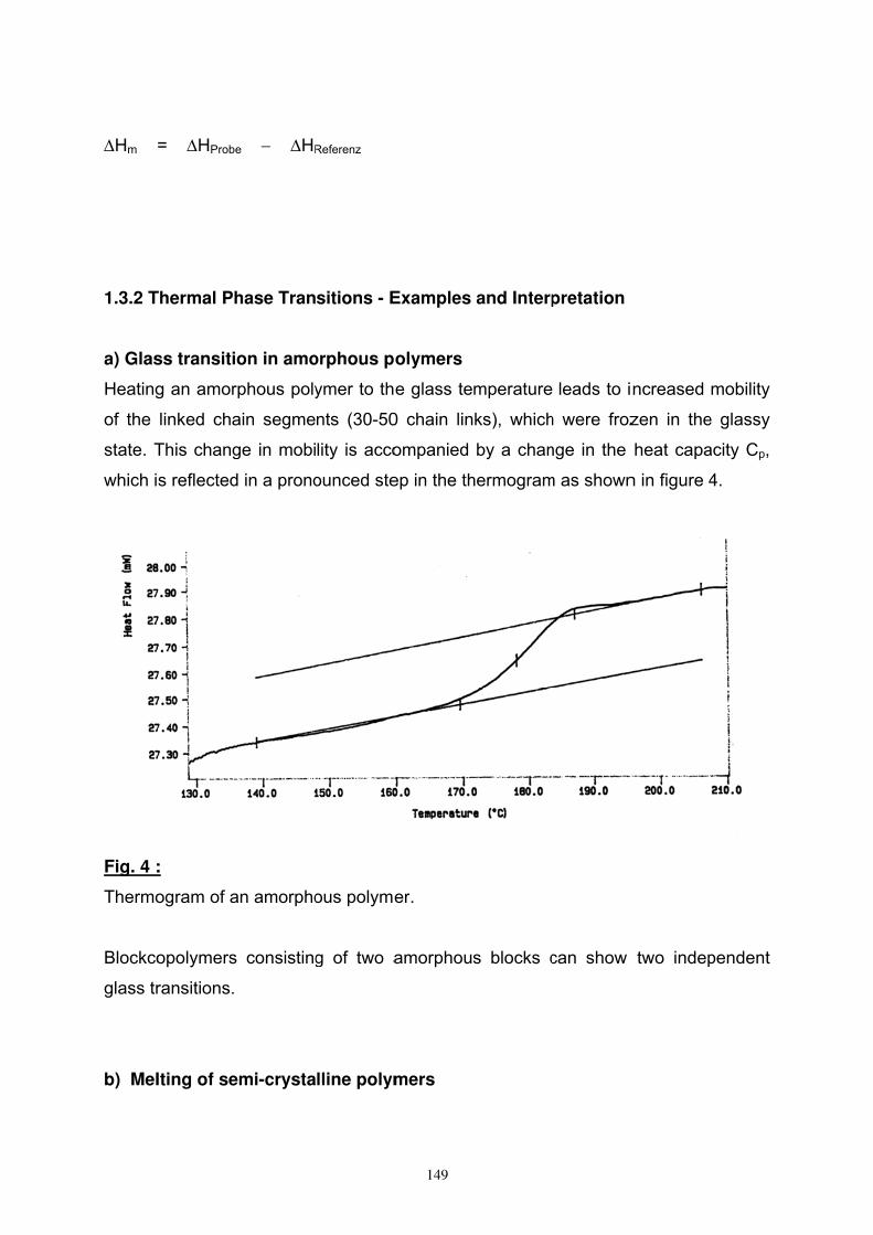
Hm

1.3.2 T

a) Glas

Heating

of the

state. T

which i

Fig. 4 :

Thermo

Blockco

glass tr

b) Mel

= HProbe

Thermal Ph

ss transiti

g an amor

linked cha

This chang

s reflected

:

ogram of a

opolymers

ransitions.

lting of se

e HR

hase Tran

on in amo

rphous poly

ain segme

ge in mobi

d in a prono

an amorpho

consisting

emi-crysta

Referenz

sitions - E

orphous p

ymer to th

nts (30-50

lity is acco

ounced ste

ous polyme

g of two a

lline polym

149

Examples

olymers

e glass te

0 chain lin

ompanied

ep in the th

er.

amorphous

mers

and Interp

mperature

ks), which

by a chan

hermogram

s blocks c

pretation

leads to i

h were froz

nge in the

m as shown

can show

ncreased

zen in the

heat capa

n in figure 4

two indep

mobility

e glassy

acity Cp,

4.

pendent

Semi-c

crystals

thickne

fully ex

is why

the so-

crystal.

crystal’

melting

The m

crystall

This re

surface

infinite

crystalline

s), where

ess of abou

xtended ch

the experi

-called equ

. The redu

s chemica

g temperatu

elting poin

ites l (thick

elation is d

e tension o

fully exten

polymers t

the indiv

ut 60 – 300

hains and t

mentally d

uilibrium m

uction of th

al potential

ure of an id

nt of sem

kness of la

T

escribed b

of the lame

nded chain

typically s

vidual lam

0 Å (length

thus the su

determined

melting poi

he surface

and leads

deal crysta

T

i-crystallin

amellae wit

T Tm m 0

by the Tho

ellaes’ top

crystal H

150

how a lam

ellae inclu

h period L

urface to v

d melting p

int Tm

0 valid

e energy (s

s to a melt

al is given

TH

Sm

m

0

e polymer

thout amor

c

1(

mson equ

surface ,

Hm

0 and the

mellar struc

uding the

). An ideal

olume rati

point Tm of

d for the i

surface of

ting point r

by:

Hm

m

0

0

rs depend

rphous fold

H lm

0

2 )

ation (see

the specif

e density o

cture (Fig.

amorphou

l polymer c

o is compa

polymers

nfinite fully

f the lamel

reduction

ds on the

ding region

)

above), w

fic enthalp

f the crysta

1b; chain

us parts

crystal con

arably sma

always lie

y extende

llae) chan

T Tm

o

thickness

ns).

which inclu

py of meltin

alline regio

n folded

have a

nsists of

all. That

s below

d chain

ges the

Tm

. The

s of the

des the

ng of an

ons c.

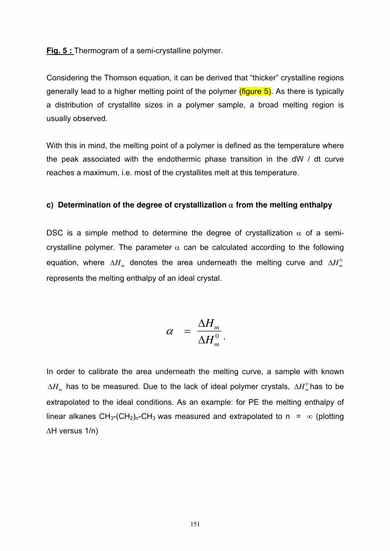
151

Fig. 5 : Thermogram of a semi-crystalline polymer.

Considering the Thomson equation, it can be derived that “thicker” crystalline regions

generally lead to a higher melting point of the polymer (figure 5). As there is typically

a distribution of crystallite sizes in a polymer sample, a broad melting region is

usually observed.

With this in mind, the melting point of a polymer is defined as the temperature where

the peak associated with the endothermic phase transition in the dW / dt curve

reaches a maximum, i.e. most of the crystallites melt at this temperature.

c) Determination of the degree of crystallization from the melting enthalpy

DSC is a simple method to determine the degree of crystallization of a semi-

crystalline polymer. The parameter can be calculated according to the following

equation, where Hm

denotes the area underneath the melting curve and 0

mH

represents the melting enthalpy of an ideal crystal.

H

H

m

m

0 ,

In order to calibrate the area underneath the melting curve, a sample with known

Hm

has to be measured. Due to the lack of ideal polymer crystals, 0

mH has to be

extrapolated to the ideal conditions. As an example: for PE the melting enthalpy of

linear alkanes CH3-(CH2)n-CH3 was measured and extrapolated to n = (plotting

H versus 1/n)

152

2. Experimental Section

Table 1: Measurement procedure for the investigated samples:

Measurement

No.

Sample Amount Starting

temperature

Final

temperature

Heating rate

[mg] [°C] [°C] [K/min]

1 Indium 5.525 130 170 10

2 it - PS 50

270

50

270

50

270

10

10

10

3 PET 30 300 20

300

30

30

300

10

10

Enthalpies of melting Hm

0 :

Indium: 28.2 J/g

it - PS: 86.8 J/g

Tonset (Indium) = 156.6 °C

153

3. Data Evaluation

1) Display the experimental parameters (see table 1) and values obtained from the

different measurements (melting and glass transition temperatures, transition

enthalpies) in a table. Correct the temperatures by subtracting the indium onset.

Correct the enthalpies by multiplying with the factor (theoretical / measured) derived

from the indium measurement. Display the corrected values in a table.

2) Discuss the profile of the indium heating curve.

3) Discuss the it – PS measurement.

Determine the degree of crystallization of the it – PS sample.

4) Discuss the PET measurement.

Determine the degree of crystallization of the PET sample (search for the

corresponding Hm

0 value in the literature).

154

4. Questions

1) Isotactic polypropylene crystallizes in a „31 - helix“ structure. What is the

meaning of the coefficents? (Polybutene: 85 - helix)

2) Describe synthesis routes to isotactic polypropylene and isotactic polystyrene!

3) How does the degree of crystallinity affect the mechanical properties of the

polymers?

4) Describe possible solid state structures of blockcopolymers comprising

crystallizable and non-crystallizable blocks (e.g. PE - PS - PE)?

5) Rapid quenching of a crystallizable polymer from melt leads to a polymer

glass. By which methods can the glass be transformed into the semi-

crystalline state?

Documents

Laboratory Course Polymer Chemistry - Universität … · Give an example of an analytical polymer ... reactions between bifunctional or polyfunctional ... or with the monomeric compound,