Laboratory 1 Tensile Test of Materialsteacher.buet.ac.bd/bazlurrashid/222_2017_Jan/222_e01.pdfThe tensile test measures the resistance of a material to a static or slowly applied force

MME222/Jan 17 Term/Expt. 01: Tensile Testing of Materials Page 1 of 16

Department of Materials and Metallurgical Engineering

Bangladesh University of Engineering and Technology, Dhaka

MME222 Materials Testing Sessional 1.50 Credits

January 2017 Term

Laboratory 1

Tensile Test of Materials

1. Objective

The tensile test measures the resistance of a material to a static or slowly applied force. This laboratory

experiment is designed to demonstrate the procedure used for obtaining mechanical properties as modulus

of elasticity, yield strength, ultimate tensile strength (UTS), toughness, uniform elongation, elongation and

reduction in area at rupture. After completion of this experiment, students should be able to

1.1 understand the principle of a uniaxial tensile testing and gain their practices on operating the tensile

testing machine to achieve the required tensile properties following a specific standard,

1.2 explain load-extension and stress-strain relationships and represent them in graphical forms,

1.3 evaluate the values of ultimate tensile strength, yield strength, elongation at failure, and Young’s

Modulus of the selected materials when subjected to uniaxial tensile loading, and

1.4 explain deformation and fracture characteristics of different metallic and non-metallic materials when

subjected to uniaxial tensile loading.

2. Materials and Equipment

2.1 Tensile specimens

2.2 Universal testing machine (UTM)

2.3 Micrometer or vernia calliper

2.4 Steel scale

2.5 Stereoscope

3. Experimental Procedure

3.1 Measure dimensions (diameter or width and thickness) of the specimen provided and record in Table

1.1. Mark the location of the gauge length along the parallel length of reduced cross section of each

specimen for subsequent observation of necking and strain measurement.

3.2 Observe and record the type of tensile testing machine to be used for the experiment. Fit the specimen

on to the machine. Note the mode of testing and strain rate to be used for the test. Carry on testing

until fracture of the sample.

3.3 After the specimen is broken, join the two broken pieces of the specimen together, held them firmly,

and then measure the final gauge length and the final diameter of the broken pieces.

3.4 If the machine is operated manually, record load and extension for the construction of load-extension

and stress-strain curve of the specimen.

3.5 For automated or computer software-operated machine, take the raw data and import it to Microsoft

Excel or any other similar programme.

3.6 Before plotting the chart, use the calibration chart or formula (which can be found to be attached to

the machine) of the machine to calculate the actual value of the load from the observed value.


4. Results

4.1 Plot a load - elongation curve for each specimen.

4.2 Determine the engineering stress-strain curve and the true stress- true strain curve.

4.3 Determine Young's modulus, yield strength, ultimate tensile strength, elongation at failure, and

reduction in area. Determine the mathematical expression for the true stress true strain curve for the

second material.

4.4 Observe the fracture surfaces of broken specimens using stereoscope, and sketch and describe the

fractured surface.

4.5 Identify the fracture mode, i.e. ductile or brittle and explain the reasons.

5. Discussion

5.1 If the identification of material of the sample is given, compare your test results of strength and

ductility with its book values. Discuss the reasons for the significant difference, if any.

5.2 Answer the following questions:

(a) Discuss the variations in nature of the load-extension (or, stress-strain) graphs of steel, cast iron

and aluminium.

(b) Explain briefly the tensile behaviour of polymeric material. Why do you think it is different from

that of metallic material?

(c) Discuss the effect of specimen shape and size on tensile properties of material.

(d) What is the approximate value of Poisson's ratio for metals? What is the physical significance of

Poisson’s ratio, i.e. what does it represent resistance to?

(e) What % elongation and % reduction in area measures of?

(f) What is the area under the stress-strain curve equivalent to? What does the area under the elastic

portion of the stress-strain represent?

(g) What is work hardening exponent (n)? How is this value related to the ability of metal to be

mechanically formed?

(h) Both yield strength and ultimate tensile strength exhibit the ability of a material to withstand a

certain level of load. Which parameter do you prefer to use as a design parameter for a proper

selection of materials for structural applications? Explain.


Table 1.1: Data Sheet

Symbol Unit Value

Sample identification 1 2 3 Average

Description of material

Initial diameter of sample 𝐷0 mm

Initial width of sample 𝑊0 mm

Initial thickness of sample 𝑇0 mm

Initial cross-sectional area of sample 𝐴0 mm2

Initial gauge length of sample 𝐿0 mm

Final diameter of sample 𝐷𝑓 mm

Final width of sample 𝑊𝑓 mm

Final thickness of sample 𝑇𝑓 mm

Final cross-sectional area of sample 𝐴𝑓 mm2

Final gauge length of sample 𝐿𝑓 mm

Young Modulus 𝐸 = tan 𝜃 GPa

Yield load or 0.1/0.2/0.5 offset load 𝑃𝑦 or 𝑃0.2 kN

Yield Strength or 0.1/0.2/0.5 Proof Strength 𝜎𝑦 or 𝜎0.2 MPa

Maximum load 𝑃𝑚𝑎𝑥 kN

Ultimate Tensile Strength 𝜎𝑈𝑇𝑆 MPa

Fracture load 𝑃𝑓 kN

Fracture Strength 𝜎𝑓 MPa

Elongation at Failure 𝐸 %

Reduction in Area 𝑅𝐴 %

Work hardening exponent 𝑛

Modulus of resilience 𝑈𝑅

Tensile toughness 𝑈𝑇

Fracture Mode

**Provide all calculations in separate pages.


6. Theoretical Background

6.1 Introduction

Uniaxial tensile test is known as a basic and universal engineering test for determining the mechanical

properties of materials, such as strength, ductility, toughness, elastic modulus, and strain hardening

capability. These important parameters obtained from the standard tensile testing are useful for the

selection of engineering materials for any applications required.

The tensile testing is carried out by applying longitudinal or axial load at a specific extension rate to a

standard tensile specimen with known dimensions (gauge length and cross sectional area perpendicular to

the load direction) till failure. The applied tensile load and extension are recorded during the test for the

calculation of stress and strain. A range of universal standards provided by Professional societies such as

American Society of Testing and Materials (ASTM), British standard, JIS standard and DIN standard

provides testing are selected based on preferential uses. Each standard may contain a variety of test

standards suitable for different materials, dimensions and fabrication history. For instance, ASTM E8: is a

standard test method for tension testing of metallic materials and ASTM B557 is standard test methods of

tension testing wrought and cast aluminium and magnesium alloy products.

A standard specimen is prepared in a round or a square section along the gauge length as shown in Fig. 6.1

(a) and (b) respectively, depending on the standard used. Normally, the cross section is circular, but

rectangular specimens are also used. This ―dogbone‖ specimen configuration was chosen so that, during

testing, deformation is confined to the narrow centre region (which has a uniform cross section along its

length) and also to reduce the likelihood of fracture at the ends of the specimen. The standard diameter of

the reduced section (also known as the gauge diameter) is 12.5 mm (0.505 in.) and the standard value of

gauge length is 50 mm (2.0 in.). The initial gauge length 𝐿0 is standardized (in several countries) and varies

with the diameter (𝐷0) or the cross-sectional area (𝐴0) of the specimen as listed in Table 6.1. This is because

if the gauge length is too long, the % elongation might be underestimated in this case. Both ends of the

specimens should have sufficient length and a surface condition such that they are firmly gripped during

testing. Any heat treatments should be applied on to the specimen prior to machining to produce the final

specimen readily for testing. This has been done to prevent surface oxide scales that might act as stress

concentration which might subsequently affect the final tensile properties due to premature failure. There

might be some exceptions, for examples, surface hardening or surface coating on the materials. These

processes should be employed after specimen machining in order to obtain the tensile properties results

which include the actual specimen surface conditions.

12.5 mm Round Specimen 12.5 mm Plate Specimen

L0 – Gauge length 50.00.1 L0 – Gauge length 50.00.1

D0 – Gauge diameter 12.50.2 W – Width 12.50.2

R – Radius of fillet, min. 10 T – Thickness

A – Length of reduced section, min. 57 R – Radius of fillet, min. 12.5

L – Overall length 200

A – Length of reduced section, min. 57

B – Length of grip section 50

C – Width of grip section, approx. 20

Figure 6.1: Standard tensile specimens.

L0

D0

A

R

L0

W

A

R

B

L

T

C


Table 6.1: Dimensional relationships of tensile specimens used in different countries.

Specimen

Type

ASTM Standards

(USA)

BS Standards

(Great Britain)

DIN Standards

(Germany)

Sheet 𝐿0 𝐴0 4.5 5.65 11.3

Rod 𝐿0 𝐷0 4.0 5.00 10.0

Equipment used for tensile testing range from simple, hand-actuated devices to complex, servo-hydraulic

systems controlled through computer interfaces. Common configurations (for example, as shown in Fig.

6.2) involve the use of a general purpose device called a universal testing machine. Modern test machines

fall into two broad categories: electro (or servo) mechanical (often employing power screws) and servo-

hydraulic (high-pressure hydraulic fluid in hydraulic cylinders). Figure 6.3(a) illustrates a relatively simple

screw-driven machine using large two screws to apply the load whereas Fig. 6.3(b) shows a hydraulic

testing machine using the pressure of oil in a piston for load supply. These types of machines can be used

not only for tension, but also for compression, bending and torsion tests.

Figure 6.2: Example of a modern, closed-loop servo-hydraulic universal test machine.

Digital, closed loop control (e.g., force, displacement, strain, etc.) along with computer interfaces and user

friendly software are common. Various types of sensors are used to monitor or control force (e.g., strain

gage-based ―load‖ cells), displacement (e.g., linear variable differential transformers ( LVDT’s) for stroke of

the test machine), and strain (e.g., clip-on strain-gauged based extensometers). In addition, controlled

environments can also be applied through self-contained furnaces, vacuum chambers, or cryogenic

apparatus. Depending on the information required, the universal test machine can be configured to provide

the control, feedback, and test conditions unique to that application.

General techniques utilized for measuring loads and displacements employs sensors providing electrical

signals. Load cells are used for measuring the load applied while strain gauges are used for strain

measurement. A Change in a linear dimension is proportional to the change in electrical voltage of the

strain gauge attached on to the specimen.


(a) (b)

Figure 6.3: Schematics showing (a) a screw driven machine and (b) a hydraulic testing machine.

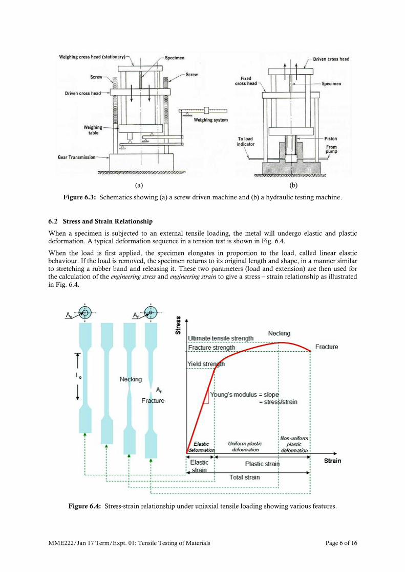
6.2 Stress and Strain Relationship

When a specimen is subjected to an external tensile loading, the metal will undergo elastic and plastic

deformation. A typical deformation sequence in a tension test is shown in Fig. 6.4.

When the load is first applied, the specimen elongates in proportion to the load, called linear elastic

behaviour. If the load is removed, the specimen returns to its original length and shape, in a manner similar

to stretching a rubber band and releasing it. These two parameters (load and extension) are then used for

the calculation of the engineering stress and engineering strain to give a stress – strain relationship as illustrated

in Fig. 6.4.

Figure 6.4: Stress-strain relationship under uniaxial tensile loading showing various features.


The engineering stress (or, nominal stress), 𝜎, is defined as the ratio of the applied load, P, to the original

cross-sectional area, A0, of the specimen:

𝜎 = 𝑃

𝐴0

(6.1)

The engineering strain, 𝜀, is defined as a ratio of the change in length to its original length

𝜀 = 𝐿 − 𝐿0

𝐿0

= Δ𝐿

𝐿0

(6.2)

where 𝐿0 is the original length of the specimen, and 𝐿 is the instantaneous length of the specimen.

The unit of the engineering stress is megapascal (MPa) according to the SI Metric Unit where 1 MPa = 106

N/m2 whereas the unit of psi (pound per square inch) can also be used in the FPS system.

It can be noted here that, since the stress is obtained by dividing load with a constant (i.e., the original area

of the specimen) and the strain is obtained by dividing extension (or deformation) with another constant

(i.e., the original gauge length of the specimen), instead of stress – strain diagram, the similar deformation

sequence in a tensile test can also be represented in a load – deformation diagram.

Many materials exhibit stress-strain curves considerably different from that mentioned in Fig. 6.4. Low carbon-steels or mild steels, for example, show two distinct yield points (a.k.a upper yield point and lower

yield point) in their stress – strain diagrams, Fig. 6.5. In addition, the stress-strain curve for more brittle

materials, such as cast iron, fully hardened high-carbon steel, or ceramics show more linearity and much

less nonlinearity of the ductile materials. Little ductility is exhibited with these materials, and they fracture

soon after reaching the elastic limit. Because of this property, greater care must be used in designing with

brittle materials. The effects of stress concentration are more important, and there is no large amount of

plastic deformation to assist in distributing the loads.

Figure 6.5: Different schematic stress – strain diagram of different types of materials.

It can be note from the above diagram that, the stress – strain curve of normal (semi-crystalline) polymer

differs dramatically from other ductile metals in that the neck does not continue shrinking until the

specimen fails. Rather, the material in the neck stretches and propagates until it spans the full gage length

of the specimen, a process called drawing. This leads to localised strengthening of the materials and

subsequent upward trend of the stress-strain curve before failure.

Young’s Modulus

During elastic deformation, the engineering stress-strain relationship follows the Hook's Law and the slope of the curve indicates the modulus of elasticity or the Young’s modulus, E:


𝐸 = 𝜎

𝜀 (6.3)

This linear relationship is known as Hooke’s law. Note in Eq. (6.3) that, because engineering strain is

dimensionless, E has the same units as stress. The modulus of elasticity is the slope of the elastic portion of

the curve and hence indicates the stiffness of the material. The higher the E value, the higher is the load

required to stretch the specimen to the same extent, and thus the stiffer is the material. Young's modulus is

of importance where deflection of materials is critical for the required engineering applications. This is for

examples: deflection in structural beams is considered to be crucial for the design in engineering

components or structures such as bridges, building, ships, etc. The applications of tennis racket and golf

club also require high values of spring constants or Young’s modulus values.

The elongation of the specimen under tension is accompanied by lateral contraction; this effect can easily

be observed by stretching a rubber band. The absolute value of the ratio of the lateral strain to the

longitudinal strain is known as Poisson’s ratio and is denoted by the symbol 𝜈. For many metals and other

alloys, values of Poisson’s ratio range between 0.25 and 0.35.

Yield Strength and Proof Stress

As the load is increased, the specimen begins to undergo nonlinear elastic deformation at a stress called the proportional limit. At that point, the stress and strain are no longer proportional, as they were in the linear

elastic region, but when unloaded, the specimen still returns to its original shape. Permanent (plastic)

deformation occurs when the yield strength of the material is reached. The yield strength, 𝜎𝑦 , can be

obtained by dividing the load at yielding (Py) by the original cross-sectional area of the specimen (A0):

𝜎𝑦 = 𝑃𝑦

𝐴0

(6.4)

The yield point can be observed directly from the load-extension curve of the BCC metals such as iron and

steel or in polycrystalline titanium and molybdenum, and especially low carbon steels (see Fig. 6.6(b)). The

yield point elongation phenomenon shows the upper yield point followed by a sudden reduction in the

stress or load till reaching the lower yield point. At the yield point elongation, the specimen continues to

extend without a significant change in the stress level. Load increment is then followed with increasing

strain. This yield point phenomenon is associated with a small amount of interstitial or substitutional

atoms. This is for example in the case of low-carbon steels, which have small atoms of carbon and nitrogen

present as impurities. When the dislocations are pinned by these solute atoms, the stress is raised in order

to overcome the breakaway stress required for the pulling of dislocation line from the solute atoms. This

dislocation pinning is related to the upper yield point as indicated in Fig. 6.6(b). If the dislocation line is

free from the solute atoms, the stress required to move the dislocations then suddenly drops, which is

associated with the lower yield point. Furthermore, it was found that the degree of the yield point effect is

affected by the amounts of the solute atoms and is also influenced by the interaction energy between the

solute atoms and the dislocations. For metals that display this effect, the yield strength is taken as the

average stress that is associated with the lower yield point because it is well defined and relatively

insensitive to the testing procedure.

For soft and ductile materials such as aluminium, it may not be easy to determine the exact location on the

stress–strain curve at which yielding occurs, because the slope of the curve begins to decrease slowly above the proportional limit. Therefore, Py is usually defined by drawing a line with the same slope as the linear

elastic curve, but that is offset by a strain of 0.002, or 0.2% elongation. The yield stress is then defined as the stress where this offset line intersects the stress–strain curve and renamed as the proof stress. This simple

procedure is shown in Fig. 6.6(a). The yield strength therefore has to be calculated from the load at 0.2%

strain divided by the original cross-sectional area as follows:

𝜎0.2% = 𝑃0.2%

𝐴0

(6.5)

Offset at different values can also be made depending on specific uses: for instance; at 0.1 or 0.5% offset.

The yield strength of soft materials exhibiting no linear portion to their stress-strain curve such as soft

copper or gray cast iron can be defined as the stress at the corresponding total strain, for example, = 0005.


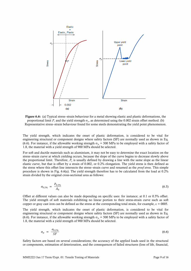
Figure 6.6: (a) Typical stress–strain behaviour for a metal showing elastic and plastic deformations, the

proportional limit P, and the yield strength y, as determined using the 0.002 strain offset method. (b)

Representative stress–strain behaviour found for some steels demonstrating the yield point phenomenon.

The yield strength, which indicates the onset of plastic deformation, is considered to be vital for

engineering structural or component designs where safety factors (SF) are normally used as shown in Eq.

(6.6). For instance, if the allowable working strength w = 500 MPa to be employed with a safety factor of

1.8, the material with a yield strength of 900 MPa should be selected.

For soft and ductile materials such as aluminium, it may not be easy to determine the exact location on the

stress–strain curve at which yielding occurs, because the slope of the curve begins to decrease slowly above the proportional limit. Therefore, Py is usually defined by drawing a line with the same slope as the linear

elastic curve, but that is offset by a strain of 0.002, or 0.2% elongation. The yield stress is then defined as the stress where this offset line intersects the stress–strain curve and renamed as the proof stress. This simple

procedure is shown in Fig. 6.6(a). The yield strength therefore has to be calculated from the load at 0.2%

strain divided by the original cross-sectional area as follows:

𝜎0.2% = 𝑃0.2%

𝐴0

(6.5)

Offset at different values can also be made depending on specific uses: for instance; at 0.1 or 0.5% offset.

The yield strength of soft materials exhibiting no linear portion to their stress-strain curve such as soft

copper or gray cast iron can be defined as the stress at the corresponding total strain, for example, = 0005.

The yield strength, which indicates the onset of plastic deformation, is considered to be vital for

engineering structural or component designs where safety factors (SF) are normally used as shown in Eq.

(6.6). For instance, if the allowable working strength w = 500 MPa to be employed with a safety factor of

1.8, the material with a yield strength of 900 MPa should be selected.

𝜎𝑤 = 𝜎0.2%

𝑆𝐹 (6.6)

Safety factors are based on several considerations; the accuracy of the applied loads used in the structural

or components, estimation of deterioration, and the consequences of failed structures (loss of life, financial,


economical loss, etc.). Generally, buildings require a safety factor of 2, which is rather low since the load

calculation has been well understood. Automobiles has safety factor of 2 while pressure vessels utilize

safety factors of 3-4.

Ultimate Tensile Strength

As the specimen begins to elongate under a continuously increasing load, its cross-sectional area decreases

permanently and uniformly throughout its gage length. Beyond yielding, continuous loading leads to an

increase in the stress required to permanently deform the specimen as shown in the engineering stress-strain curve. At this stage, the specimen is strain hardened or work hardened. The degree of strain hardening

depends on the nature of the deformed materials, crystal structure and chemical composition, which affects

the dislocation motion. FCC structure materials having a high number of operating slip systems can easily

slip and create a high density of dislocations. Tangling of these dislocations requires higher stress to

uniformly and plastically deform the specimen, therefore resulting in strain hardening. As the load is

increased further, the engineering stress eventually reaches a maximum and then begins to decrease (Fig.

6.4). The maximum engineering stress is called the tensile strength, or ultimate tensile strength (UTS), of

the material.

𝜎𝑇𝑆 = 𝑃𝑚𝑎𝑥

𝐴0

(6.7)

If the specimen is loaded beyond its ultimate tensile strength, it begins to neck, or neck down. This can be

observed by a local reduction in the cross-sectional area of the specimen generally observed in the centre of

the gauge length. As the test progresses, the engineering stress drops further and the specimen finally

fractures at the necked region (Fig. 6.4); the engineering stress at fracture is known as the breaking or fracture stress.

𝜎𝑓 = 𝑃𝑓

𝐴0

(6.8)

Tensile Ductility

An important mechanical behaviour observed during a tension test is ductility — the extent of plastic

deformation that the material undergoes before fracture. A metal that experiences very little or no plastic deformation upon fracture is termed brittle. The tensile stress–strain behaviours for both ductile and brittle

metals are schematically illustrated in Figure 6.7.

Figure 6.7: Schematic representations of tensile

stress–strain behaviour for brittle and ductile metals

loaded to fracture.

There are two common measures of ductility. The first is the total elongation of the specimen at failure, which

measures the percentage of plastic strain at fracture and is given by

%𝐸𝐿 = 𝐿𝑓 − 𝐿0

𝐿0

x 100 = Δ𝐿

𝐿0

x 100 (6.9)


where Lf and L0 are measured as shown in Fig. 6.4. We should note here that the elongation is calculated as

a percentage and it depends on the original gage length of the specimen, as a significant proportion of the

plastic deformation at fracture is confined to the neck region of the specimen during necking just prior to fracture. The shorter the L0, the greater the fraction of total elongation from the neck and, consequently, the

higher the value of %EL. Therefore, L0 should be specified when percent elongation values are cited.

The second measure of ductility is the reduction of area, given by

%𝑅𝐴 = 𝐴0 − 𝐴𝑓

𝐴0

x 100 = Δ𝐴

𝐿0

x 100 (6.10)

where A0 and Af are, respectively, the original and final (fracture) cross-sectional areas of the test specimen.

Note that %RA is not sensitive to gage length and is somewhat easier to obtain, only a micrometer is

required. Furthermore, for a given material, the magnitudes of %EL and %RA will, in general, be different.

Reduction of area and elongation are generally interrelated, as shown in Fig. 6.8 for some typical metals.

Thus, the ductility of a piece of chalk is zero, because it does not stretch at all or reduce in cross section; by

contrast, a ductile specimen, such as putty or chewing gum, stretches and necks considerably before it fails.

Most metals possess at least a moderate degree of ductility at room temperature; however, some become

brittle as the temperature is lowered.

Figure 6.8: Approximate relationship between elongation and tensile reduction of area

for various groups of metals.

Knowledge of the ductility of materials is important for at least two reasons. First, it indicates to a designer

the degree to which a structure will deform plastically before fracture. Second, it specifies the degree of

allowable deformation during fabrication operations. We sometimes refer to relatively ductile materials as

being ―forgiving,‖ in the sense that they may experience local deformation without fracture, should there

be an error in the magnitude of the design stress calculation. Brittle materials are approximately considered

to be those having a fracture strain of less than about 5%.

True Stress and True Strain

It should be realized that the stress-strain curves just discussed, using engineering quantities, are fictitious

in the sense that the and are based on areas and lengths that no longer exist at the time of measurement.

From Fig. 6.4, the decline in the stress necessary to continue deformation past the maximum point seems

to indicate that the metal is becoming weaker. This is not at all the case; as a matter of fact, it is increasing

in strength. However, the cross sectional area is decreasing rapidly within the neck region, where

deformation is occurring. This results in a reduction in the load-bearing capacity of the specimen. The

stress, as computed from Eq. 6.1, is on the basis of the original cross-sectional area before any deformation

and does not take into account this reduction in area at the neck. To correct this situation true stress (T )

and true strain (T ) quantities are used.

True stress T is defined as the load P divided by the actual (instantaneous, hence true) cross-sectional area

Ai over which deformation is occurring, or


𝜎𝑇 = 𝑃

𝐴𝑖

(6.11)

For true strain, first consider the elongation of the specimen as consisting of increments of instantaneous

change in length. Then, using calculus, it can be shown that the true strain (natural or logarithmic strain) is

calculated as

𝜀𝑇 = 𝑑𝐿

𝐿

𝐿

𝐿0

= 𝑙𝑛 𝐿

𝐿0 (6.12)

or,

𝜀𝑇 = − 𝑑𝐴

𝐴

𝐴

𝐴0

= − 𝑙𝑛 𝐴

𝐴0 (6.13)

Note from Eqs. (6.2) and (6.12) that for small values of strain the engineering and true strains are

approximately equal. However, they diverge rapidly as the strain increases. For example, when e = 0.1, =

0.095, and when e = 1, = 0.69. Thus, these two definitions of true strain are equivalent in the plastic

range where the material volume can be considered constant (i.e., V = AL = A0L0) during deformation.

Prior to necking, engineering values can be related to true values by noting that

𝜎𝑇 = 𝜎 1 + 𝜀 (6.14)

𝜀𝑇 = 𝑙𝑛 1 + 𝜀 (6.15)

where and are the engineering stress and strain values at a particular load. Equations 6.14 and 6.15 are

valid only to the onset of necking; beyond this point, true stress and strain should be computed from actual

load, cross-sectional area, and gauge length measurements.

A schematic comparison of engineering and true stress–strain behaviours is made in Fig. 6.9. It is worth

noting that the true stress necessary to sustain increasing strain continues to rise past the maximum point.

Coincident with the formation of a neck is the introduction of a complex stress state within the neck region

(i.e., the existence of other stress components in addition to the axial stress). As a consequence, the correct

stress (axial) within the neck is slightly lower than the stress computed from the applied load and neck cross-

sectional area. This leads to the ―corrected‖ curve in Fig. 6.9.

Figure 6.9: A comparison of typical tensile engineering stress–strain and true stress–strain behaviours.

Necking begins at point M on the engineering curve, which corresponds to M’ on the true curve. The

―corrected‖ true stress–strain curve takes into account the complex stress state within the neck region.


Work Hardening Component, n

True stress and true strain values are particularly necessary when one is working with large plastic

deformations such as large deformation of structures or in metal forming processes. In the elastic region the

relation between stress and strain is simply the linear equation

𝜎 = 𝐸𝜀 and 𝜎𝑇 = 𝐸𝜀𝑇 (6.16)

Material behaviour beyond the elastic region where stress-strain relationship is no loner linear (uniform

plastic deformation) can be shown as a power law expression as follows

𝜎𝑇 = 𝐾 𝜀𝑇 𝑛 (6.17)

where K is the strength coefficient and n is an exponent often called the strain hardening coefficient.

The strain-hardening coefficient values, n, of most metals range between 0.1-0.5. High value of the strain-

hardening coefficient indicates an ability of a metal to be readily plastically deformed under applied

stresses. This is also corresponding with a large area under the stress-strain curve up to the maximum load.

Taking log in both sides, Eq. (6.16) and (6.17) can be written as follows:

log 𝜎𝑇 = log 𝐸 + log 𝜀𝑇 (Elastic) (6.18)

log 𝜎𝑇 = log 𝐾 + 𝑛 log 𝜀𝑇 (Plastic) (6.19)

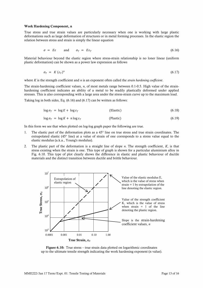
In this form we see that when plotted on log-log graph paper the following are true.

1. The elastic part of the deformation plots as a 45° line on true stress and true strain coordinates. The

extrapolated elastic (45° line) at a value of strain of one corresponds to a stress value equal to the

elastic modulus (a.k.a., Young's modulus).

2. The plastic part of the deformation is a straight line of slope n. The strength coefficient, K, is that

stress existing when the strain is one. This type of graph is shown for a particular aluminium alloy in

Fig. 6.10. This type of plot clearly shows the difference in elastic and plastic behaviour of ductile

materials and the distinct transition between ductile and brittle behaviour.

Figure 6.10: True stress – true strain data plotted on logarithmic coordinates

up to the ultimate tensile strength indicating the work hardening exponent (n value).

Value of the elastic modulus E, which is the value of stress when

strain = 1 by extrapolation of the

line denoting the elastic region.

Value of the strength coefficient

K, which is the value of stress when strain = 1 of the line denoting the plastic region.

Slope is the strain-hardening coefficient values, n

Extrapolation of

elastic region

True Strain, T

0.0001 0.001 0.01 0.10 1.00

Tru

e S

tress

,

T

107

106

105

104

103


Modulus of Resilience

Resilience is the capacity of a material to absorb energy when it is deformed elastically and then, upon unloading, to have this energy recovered. The associated property is the modulus of resilience, UR, which is

the strain energy per unit volume required to stress a material from an unloaded state up to the point of

yielding.

Computationally, the modulus of resilience for a specimen subjected to a uniaxial tension test is just the

area under the engineering stress–strain curve taken to yielding (Fig. 6.11), or

Figure 6.11: Schematic representation showing how

modulus of resilience (corresponding to the shaded

area) is determined from the tensile stress–strain

behaviour of a material.

𝑈𝑅 = 𝜎 𝑑𝜀𝜎𝑦

0

(6.20a)

Assuming a linear elastic region, we have

𝑈𝑅 = 1

2 𝜎𝑦 𝜀𝑦 =

𝜎𝑦2

2𝐸 (6.20b)

in which y is the strain at yielding.

Thus, resilient materials are those having high yield strengths and low moduli of elasticity; such alloys are

used in spring applications. The units of resilience are the product of the units from each of the two axes of

the stress–strain plot. For SI units, this is joules per cubic meter (J/m3, equivalent to Pa).

Tensile Toughness

Tensile toughness, UT, can be considered as the area under the entire stress–strain curve which indicates the

ability of the material to absorb energy in the plastic region. In other words, tensile toughness is the ability

of the material to withstand the external applied forces without experiencing failure. Engineering

applications that requires high tensile toughness is for example gear, chains and crane hooks, etc. The

tensile toughness can be estimated from an expression as follows:

𝑈𝑇 = 𝜎 𝑑𝜀𝜎𝑓

0

≈ 1

2 𝜎𝑦 + 𝜎𝑇𝑆 𝜀𝑓 (6.21)

where TS is the ultimate tensile strength, y is the yield stress and f is the strain at fracture.


6.3 Fracture Characteristics of Tested Specimens

Metals with good ductility normally exhibit a so-called cup and cone fracture characteristic observed on

either halves of a broken specimen as illustrated in Fig. 6.12. Necking starts when the stress-strain curve has

passed the maximum point where plastic deformation is no longer uniform. Across the necking area within

the specimen gauge length (normally located in the middle), microvoids are formed, enlarged and then

merged to each other as the load is increased. This creates a crack having a plane perpendicular to the

applied tensile stress. Just before the specimen breaks, the shear plane of approximately 45° to the tensile

axis is formed along the peripheral of the specimen. This shear plane then joins with the former crack to

generate the cup and cone fracture as demonstrated in Fig. 6.13. The rough or fibrous fracture surfaces

appear in grey by naked eyes.

Figure 6.12: Stages in the cup-and-cone fracture. (a) Initial necking. (b) Small cavity formation.

(c) Coalescence of cavities to form a crack. (d) Crack propagation. (e) Final shear fracture at a 45° angle

relative to the tensile direction.

Figure 6.13: (a) Cup-and-cone fracture in aluminium. (b) Brittle fracture in mild steel.


CHECKLIST FOR TENSILE REPORT

1. Neatness of bound report.

2. Organization of report in sections.

3. Introduction section:

What mechanical properties can be determined in a tensile test.

Why are tensile properties of materials important in engineering.

What properties can be determined.

4. Experimental Procedure:

Describe specimen. What measurements are made.

What tensile machine is used.

Brief detail of test, i.e. what did you do.

Give details of the recording system for data. What data is produced.

What measurements are made after the test.

5. Data Analysis:

Define all the properties you determined.

Describe the program used for data analysis.

Describe how you plot the engineering stress-strain curve.

How did you find 0.2% yield stress, UTS, true fracture stress, % elongation, % reduction in area

and other properties.

How did you determine the mathematical expression for the true stress - true strain curve.

6. Results:

Display measured values of specimens. List values of all the mechanical properties determined in

the test with correct units.

Show graphs of the stress strain curves. All axes identified with scales.

7. Discussion:

Compare alloys, which is strongest, highest ductility, etc. Compare your results with values from a

reference.

If your results are different, explain.

Answer the questions given.

8. Conclusion:

A brief summary of what you accomplished.

9. References, tables and figures.

10. Appendix

Original graph of load vs. strain correctly identified.

Documents

Laboratory 1 Tensile Test of Materialsteacher.buet.ac.bd/bazlurrashid/222_2017_Jan/222_e01.pdfThe tensile test measures the resistance of a material to a static or slowly applied force