Embed Size (px)
Citation preview

Labor Shares and Income Inequality∗
Jonathan AdamsUniversity of Chicago
Loukas KarabarbounisUniversity of Chicago and NBER
Brent NeimanUniversity of Chicago and NBER
January 2014
Abstract
The share of aggregate income paid as compensation to labor is frequently used as a
proxy for income inequality. If capital holdings are very concentrated among high income
individuals, increasing their share of GDP, all else equal, widens the gap with poorer workers.
Indeed, two striking features over the last three decades of many advanced and developing
economies are the declining labor shares in income and the rise in income inequality. The
relationship between factor shares and inequality, however, is not so simple in a richer world
with realistic features such as endogenous portfolio decisions and capital-skill complementar-
ity. In such a world, total inequality will change with (i) the labor share, (ii) the amount of
within-labor and within-capital income inequality, and (iii) the degree to which the highest
wage earners are also those earning the highest capital incomes. Macroeconomic trends and
shocks that impact any one of these three moments are likely to impact simultaneously all
of them. We develop a framework where all these terms are jointly determined and estimate
the model to clarify the roles of changing technology, policies, and factor proportions on
labor shares and total income inequality around the globe.
JEL-Codes: E21, E25, J31.
Keywords: Labor Share, Inequality, Capital Income.
∗We thank Gianluca Violante for helpful comments and discussions.

1 Introduction
The share of aggregate income paid as compensation to labor is frequently used as a proxy for
income inequality. If capital holdings are very concentrated among high income individuals,
increasing their share of GDP, all else equal, widens the gap with poorer workers. Indeed, two
striking features over the last three decades of many advanced and developing economies are
the declining labor shares in income and the rise in income inequality.
The relationship between factor shares and inequality, however, is not so simple in a richer
world with realistic features such as endogenous portfolio decisions and capital-skill comple-
mentarity. Imagine that each agents’ total income yj equals the sum of labor income ylj and
capital income ykj . The coefficient of variation (CV ) of total income in this economy, a standard
measure of inequality, can generally be decomposed as:1
CV (y) = sLρ(yl)CV
(yl)
+ (1− sL) ρ(yk)CV
(yk). (1)
We use sL to denote labor’s share of aggregate income, ρ(yl) and ρ(yk) to denote the correlation
of labor and capital income with total income, and CV(yl)
and CV(yk)
to measure within-
labor and within-capital income inequality. Total inequality will change with the labor share,
labor or capital income inequality, and the degree to which the highest wage earners are also
those earning the highest capital incomes. Macroeconomic trends and shocks that impact any
one term in the decomposition (1) are likely to impact simultaneously all the terms.
In this paper, we develop a framework where all these terms are jointly determined in order
to evaluate quantitatively the relationship between the changes in labor share and total income
inequality. We start with a production function with two types of capital and two types of labor
that exhibits capital-skill complementarity, as in Krusell, Ohanian, Rios-Rull, and Violante
(2000). Shocks that increase the return to capital also increase the return to skilled labor,
raising the skill premium and generating increases in within-labor income inequality. These
ingredients, however, are insufficient to analyze capital income inequality and the correlation
1See Shorrocks (1982) for a derivation of this decomposition. Under fairly general assumptions such as thenon-negativity of income, similar decompositions exist for most measures of inequality. In our model below wewill allow for negative capital incomes, but present this decomposition here to build intuition.
1

of capital and labor incomes. We therefore embed our production function into an Aiyagari
(1994) style model with heterogeneous agents, persistent idiosyncratic shocks, and incomplete
markets. Agents trade assets with each other in order to smooth consumption. Capital incomes
and labor incomes are jointly determined, and the full endogenous distribution of both income
sources proves important for understanding the response of overall inequality to many shocks.
We describe an environment with no aggregate uncertainty, calibrate it to resemble the
U.S. economy around 1980, and solve for the ergodic distribution or steady state of the model.
We consider a number of experiments where we introduce a permanent shock, solve for the
new steady state, and evaluate comparative statics relative to the pre-shock steady state.
Most shocks will simultaneously influence the within-labor income inequality, the within-capital
income inequality, and the correlation between agents’ labor and capital income, which allows
us to to analyze the joint behavior of labor share and inequality.
For example, we consider a decline in the relative price of IT capital, which is more com-
plementary to skilled than to unskilled labor. The resulting IT capital deepening increases the
skill premium and labor income inequality, as in Krusell, Ohanian, Rios-Rull, and Violante
(2000). In our baseline calibration, the shock also drives a reduction in the labor share, as
in ?, which increases the primacy of capital income inequality for overall income inequality.
Depending on the model’s calibration, this can reinforce, mute, or even reverse the conclusions
drawn about inequality relative to a framework that ignores capital income. We additionally
consider a shock to the distribution of human capital stocks, a shock that relaxes the borrowing
constraint, shocks in the tax schedule, and shocks to the depreciation rate, among others. We
generally find that the dynamics of capital income inequality are important for understanding
overall income inequality when XXX...
[TBD: mapping to the data.]
[TBD: related literature.]
2

2 Trends in Inequality and its Determinants
[TBD: Trends in overall, labor, and capital inequality.]
[TBD: Declining labor shares. Financial development. Skill stock. Etc.]
3 Model
Our model embeds the production structure of Krusell, Ohanian, Rios-Rull, and Violante (2000)
in the Aiyagari (1994) and Huggett (1996) model of heterogeneous agents with incomplete
asset markets. On the production side, the economy produces a consumption good C, an
information and communication technology (IT) capital good Xs, and a non-IT capital good
Xu. We take the consumption good to be the numeraire and set its price equal to one in each
period. On the household side, there is a measure one of heterogeneous agents that differ in
idiosyncratic labor income shocks, skill endowment, and age. Throughout our analysis, we focus
on stationary equilibria in which aggregate variables are constant. We drop time subscripts
to denote variables in the current period and we use a prime to denote variables in the next
period.
3.1 Households
Households are heterogeneous with respect to their labor income shocks z, their skill endowment
h, their age j, and their accumulated assets a. We denote the household type by (a, z, h, j) and
the distribution of households across these states by λ(a, z, h, j). We assume that the economy
is in a stationary state with constant distribution of households across these states and constant
aggregate variables. Therefore, when solving their problem households expect all prices to be
constant.
Household (a, z, h, j) is endowed with zΦ(h, j)(1−h) units of unskilled labor and zΦ(h, j)h
units of skilled labor. The skill level h takes values in the set H = {0 ≤ h1, h2, ..., hNh ≤ 1}.
Skills are drawn from the distribution πh(h|j) when households are born and are constant
over time for each household. The labor income shock z follows a Markov chain defined in
3

the set Z = {z1, z2..., zNz} and with a corresponding probability distribution πz(z′|z, h). The
dependence of this probability distribution on h allows the process for labor income shocks to
vary by skill. The function Φ(h, j) denotes a skill-age effect on household’s labor income. We
denote by n the endogenous part of household’s labor supply, and by Wu and Ws the wage
per unit of unskilled and skilled labor supply. Each household’s pre-tax labor income equals
zΦ(h, j) (Wu (1− h) +Wsh)n. Households face a constant marginal tax rate τn on their labor
income.
Households accumulate financial assets a ∈ A to smooth consumption over their life-cycle
and to insure against shocks. We denote by r the interest rate on these assets. Assets are
bounded from below by some exogenous borrowing limit ψ.
We consider an economy with a constant population of measure one. At each point of time,
there are λhj households of skill h and age j, where λhj =∫A×Z λ(a, z, h, j)dadz. Households’
age j takes values in the set J = {1, 2, ..., Nj}, where Nj denotes the maximum number of
periods that a household lives. We denote by µhj the probability that a household with skill
h and age j survives to period j + 1, with µhNj = 0. Deaths are realized at the end of each
period after households choose assets, labor, and consumption. The death rate in the aggregate
economy is∑
hj(1− µhj)λhj.
For the economy to have constant population over time, the measure of deaths must equal
the measure of births in each period. To allow our model to generate a steady state with any
arbitrary household age distribution, we allocate newborn households across various generations
(instead of only to the youngest generation). Let bhj+1 be the measure of newborns allocated
to households with skill h and age j + 1. For any j > 0, we have:
λhj+1 = µhjλhj + bhj+1, (2)
and for the first generation we have λh1 = bh1, with∑
hj bhj =∑
hj(1 − µhj)λhj. We assume
that newborn households bhj+1 are allocated across labor income shocks z and assets a with
the same distribution as households of type h that arrived from the previous period j.
Denoting by β the discount factor, we write in recursive form the problem of the household
4

(whether newborn or not) as:
v(a, z, h, j) = maxc,n,a′
{u(c, n) + βµhj
∑z′∈Z
πz(z′|z, h)v(a′, z′, h, j + 1) + (1− µhj)v(a′, j)
}, (3)
subject to the budget constraint:
c+ a′ − a = (1− τn)zΦ(h, j) (Wu (1− h) +Wsh)n+ ra+ T (a, z, h, j) +B(a, z, h, j), (4)
and the borrowing constraint:
a′ ∈ A = [ψ,∞). (5)
In the value function, v(a′, j) denotes the value that a dying household of age j derives from
leaving a bequest equal to a′. In the budget constraint, T (a, z, h, j) denotes tax revenues that
are returned to a household of type (a, z, h, j) through lump-sum transfers and B(a, z, h, j)
denotes inherited bequests.
3.2 Production
The economy produces a consumption good C, an IT capital good Xs, and a non-IT capital
good Xu. We distinguish IT and non-IT capital goods for three reasons. First, price declines of
IT goods have been particularly pronounced in recent decades, leading to significant IT capital
deepening. Second, IT goods are often operated by educated workers and therefore would be
the type of capital that would most naturally exhibit complementarity with skill in production.
Third, as we detail below, we obtain a data source which uses a consistent methodology and
definition to distinguish IT from non-IT capital goods for many countries around the world.
Our disaggregation is similar qualitatively and quantitatively to splitting capital into structures
and equipment as has been done extensively in the literature.
Good G = {C,Xs, Xu} is produced by a perfectly competitive representative firm using
a constant returns to scale technology. The production of G uses inputs of unskilled labor
(Ug), skilled labor (Sg), non-IT capital (Kgu), and IT capital (Kg
s ), where the three elements of
g = {c, s, u} correspond in order to the three elements of G. The two types of labor are rented
from households at prices Wu and Ws respectively. The two types of capital are rented from
5

intermediaries at (before-tax) rates Ru and Rs respectively. We describe the problem of the
firms that intermediate capital in Section 3.3.
Producers face a corporate tax τc on their sales net of their labor expense. The profit
maximization problem of a firm in sector G is given by:
maxUg,Sg,Kg
u,Kgs
Πg = (1− τc) (pgG−WuUg −WsS
g)− RuKgu − RsKg
s , (6)
subject to the production possibility set:
G ≤ FG =1
ξgF (Ug, Sg, Kg
u, Kgs ). (7)
The first-order conditions for profit maximization imply the equalization of the value of the
net-of-tax marginal product of each factor to the factor’s price.
Note that the only difference across the three production functions FG is the 1/ξg term,
which denotes sector-specific technology. We normalize ξc = 1. Perfect competition and con-
stant returns to scale imply that for each good the price equals the marginal cost. Therefore,
differences in the prices of the three goods are tied down to differences in the technology of
production. The price of non-IT investment relative to consumption is given by pu = ξu and
the price of IT investment relative to consumption is given by ps = ξs.
Because all producers face the same factor prices and taxes, in equilibrium the marginal
revenue products are equalized across sectors. Aggregating across sectors and using the fact
that the production functions are constant returns to scale, we show that total production and
spending, denominated in units of consumption goods, equal total payments accruing to the
factors of production:
Y = C + ξuXu + ξsXs = WuU +WsS +RuKu +RsKs. (8)
where Ru = Ru/(1− τc) and Rs = Rs/(1− τc) denote the user cost of each type of capital. In
equation (8), U and S denote the total supply of unskilled and skilled labor defined as:
U =
∫A×Z×H×J
zΦ(h, j)(1− h)n(a, z, h, j)dλ and S =
∫A×Z×H×J
zΦ(h, j)hn(a, z, h, j)dλ,
(9)
6
where n(a, z, h, j) denotes the optimal choice of labor supply.
We define the factor income shares as αLu = WuU/Y , αLs = WsS/Y , αKu = RuKu/Y , and
αKs = RsKs/Y , with αLu +αLs +αKu +αKs = 1. We define the labor share as αL = αLu +αLs
and the capital share as αK = αKu + αKs.
3.3 Intermediaries of Capital
Firms that intermediate capital purchase investment goods Xu and Xs from the final goods
producers at prices ξu and ξs respectively to augment the capital stocks:
K ′u = (1− δu)Ku +Xu and K ′s = (1− δs)Ks +Xs, (10)
where δu and δs denote the depreciation rates. The intermediaries rent the two types of capital
to all final goods producers at before-tax rates of Ru and Rs respectively.
In each period, intermediaries maximize the cum-dividend value of the firm W . Let D
denote the dividends paid by the intermediary, which are discounted at rate ζ. The value of
the firm is:
W (Ku, Ks) = max{K′u,K′s}
D + ζW (K ′u, K′s), (11)
where the firm pays out its cash flows as dividends:
D = RuKu + RsKs − ξuXu − ξsXs. (12)
Intermediaries maximize the value in (11) subject to the capital accumulation equations in
(10). We focus on a stationary state in which the discount factor is ζ = 1/(1+r). In stationary
state, the first-order conditions for value maximization yield the following expressions that
relate the before-tax rental rate of each capital stock to the price of investment goods, the
interest rate, and the depreciation rate:
Ru = ξu (r + δu) and Rs = ξs (r + δs) . (13)
Intermediaries are owned by a mutual fund with which households invest all of their finan-
cial assets (a > 0) or from which households have borrowed and generated all their financial
7

liabilities (a < 0). The aggregate of all financial assets is used to purchase the firm that
intermediates capital.
Equilibrium in the asset market requires that the value of funds raised by the mutual fund
from the household at any given time (new shareholder equity in the mutual fund’s balance
sheet) equals the ex-dividend value of its newly purchased shares in the intermediaries at that
time (new assets on the mutual fund’s balance sheet). Using the fact that in stationary state
we have Xu = δuKu and Xs = δsKs together with the definition of dividends in (12), we show
that the ex-dividend value Q of the intermediary firm equals the value of the capital stock:
Q = W −D = ξuKu + ξsKs. (14)
This leads to the equilibrium condition in the asset market:∫A×Z×H×J
adλ = Q = ξuKu + ξsKs. (15)
Equation (15) says that the supply of financial assets from households must equal the
demand for capital from all final goods producers when expressed in terms of consumption
goods. Finally, we note that in stationary state dividends equal D = rQ, so that r equals the
rate of return on the value of the capital stock.
3.4 Equilibrium
We define a stationary equilibrium for the economy as a household value function v(a, z, h, j),
household policy functions c(a, z, h, j), a′(a, z, h, j), and n(a, z, h, j), transfers T (a, z, h, j) and
bequests B(a, z, h, j), intermediary value function W (Ku, Ks), a time-invariant distribution of
households over states λ(a, z, h, j), time-invariant interest rate r, wages Wu and Ws, prices pu
and ps, and user costs of capital Ru and Rs, time-invariant stocks of capital Ku and Ks and
labor U and S, and time-invariant aggregate consumption C, and investments Xu and Xs such
that:
1. Taking as given the equilibrium r, Wu, and Ws, and T (a, z, h, j) and B(a, z, h, j), the value
function v(a, z, h, j) and the policy functions c(a, z, h, j), a′(a, z, h, j), and n(a, z, h, j),
solve the household’s problem in equations (3)-(5).
8

2. In each sector, the price of the final good equals the marginal cost. Normalizing the price
of consumption goods to pc = 1 we take:
pu = ξu, (16)
ps = ξs. (17)
3. Taking as given the equilibrium prices pu and ps, wages Wu and Ws, and user costs Ru
and Rs, production decisions maximize profits:
∂F (U, S,Ku, Ks)
∂U= Wu, (18)
∂F (U, S,Ku, Ks)
∂S= Ws, (19)
∂F (U, S,Ku, Ks)
∂Ku= Ru, (20)
∂F (U, S,Ku, Ks)
∂Ks= Rs. (21)
4. Taking as given prices pu and ps and the interest rate r, capital accumulation decisions
maximize W (Ku, Ks) and imply before-tax rental rates for the capital stocks given by
equation (13).
5. Markets for consumption and investment goods clear:
C =
∫A×Z×H×J
c(a, z, h, j)dλ, (22)
Xu = δuKu, (23)
Xs = δsKs. (24)
6. The government’s budget is balanced:
T = τn (WuU +WsS) + τc (Y −WuU −WsS) =
∫A×Z×H×J
T (a, z, h, j)dλ. (25)
7. Aggregate bequests are given by:
B =
∫A×Z×H×J
(1− µhj)a′(a, z, h, j)dλ =
∫A×Z×H×J
B(a, z, h, j)dλ. (26)
9
8. The goods market clearing condition (8), the labor market clearing condition (9), and the
asset market clearing condition (15) hold.
9. The stationary distribution of households across states, λ(a, z, h, j), is consistent with
household optimization, the transition probabilities for the labor income shocks, and the
evolution of demographics. Given some initial distribution λ(a, z, h, 1) we have:
λ(a′, z′, h, j + 1) = µhj∑z∈Z
πz(z′|z, h)
∫a∈A
Ia′λ(a, z, h, j)da+ bhj+1λ(a′, z′, h, j + 1), (27)
∀h ∈ H and for j > 0, where Ia′ = I (a′ = a′(a, z, h, j)) denotes an indicator variable
taking the value of one when next period assets equal the assets implied by the optimal
policy function under state (a, z, h, j). By multiplying the mass of newborns bhj+1 by
the probability λ(a′, z′, h, j + 1), we assume that newborns are distributed across new
assets a′ and productivity shocks z′ according to the same probability as the continuing
households. Note that this implies we can rearrange (27) and write it as:
λ(a′, z′, h, j + 1) =µhj
1− bhj+1
∑z∈Z
πz(z′|z, h)
∫a∈A
Ia′λ(a, z, h, j)da. (28)
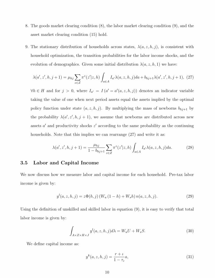
3.5 Labor and Capital Income
We now discuss how we measure labor and capital income for each household. Pre-tax labor
income is given by:
yl(a, z, h, j) = zΦ(h, j) (Wu (1− h) +Wsh)n(a, z, h, j). (29)
Using the definition of unskilled and skilled labor in equation (9), it is easy to verify that total
labor income is given by: ∫A×Z×H×J
yl(a, z, h, j)dλ = WuU +WsS. (30)
We define capital income as:
yk(a, z, h, j) =r + ι
1− τca, (31)
10

where ι is the aggregate investment rate:
ι =ξuXu + ξsXs
ξuKu + ξsKs. (32)
We choose this definition such that when aggregating capital income across households we
obtain aggregate capital income:∫A×Z×H×J
yk(a, z, h, j)dλ = RuKu +RsKs. (33)
Note that the degree of inequality across households in capital income yk is identical to that
measured using assets a or interest income ra.
4 Parameterization and Solution
In this section we describe our calibration strategy and characterize the steady state of our
baseline economy. We parameterize the model to targets chosen from U.S. data around 1980.
In the Appendix we describe the numerical solution of the model.
4.1 Benchmark Parameterization
Some parameter values are taken from other studies and are listed in Panel A of Table 1. The
remainder are estimated in the context of our model to match target moments and are listed in
Panel B. These internally calibrated parameters are jointly determined but below we associate
each parameter with the particular target moment most closely identified by that parameter.
We start by describing the production technology. Following Krusell, Ohanian, Rios-Rull,
and Violante (2000), we assume that:
F = A(Ku)φu
φs(φkK εk−1
εks + (1− φk)S
εk−1
εk
)(εkεk−1
)( εs−1
εs)
+ (1− φs)Uεs−1εs
( εsεs−1)(1−φu)
.
(34)
This production function is a Cobb-Douglas aggregator of non-IT capital Ku with the remaining
three factors. Therefore, the share of non-IT capital in income is αKu = φu. The other three
factors of production enter in the production function according to a nested CES structure.
11

We set the elasticities εs and εk to the values estimated by Krusell, Ohanian, Rios-Rull, and
Violante (2000). We then calibrate the share parameters φu, φk, and φs to match the factor
income shares αKu, αU , and αS observed in KLEMS for the United States around 1980. (Will
later replace “around”.)
We normalize overall and sector-specific productivity levels A, ξu, and ξs to 1, and we
choose the ratio of the supply of unskilled to skilled labor U/S to match the skill premium
observed in the U.S. data in 1980.2 We estimate the depreciation rates for IT and non-IT
capital from KLEMS data. The borrowing constraint ψ is internally calibrated to target the
share of households with negative asset holdings observed in the data (insert references).
Next, we calibrate household preference parameters. We assume a constant relative risk
aversion period utility function:
u(c) = (c1−γ − 1)/(1− γ), (35)
and follow Heathcote, Storesletten, and Violante (2010) in setting γ = 1.5. The discount factor
β is calibrated such that the equilibrium real interest rate matches that found in the U.S. in
1980.
Finally, we assume that the log labor endowment follows an AR(1) process:
log z′ = ρ log z + ε, (36)
with innovations following a zero-mean normal distribution, ε ∼ N (0, σ2). We set the persis-
tence parameter ρ equal to the estimate in Guvenen (2007).3 We then choose the variance of
the shocks σ2 so that the model matches the Gini coefficient on labor income in the United
States.
2We later will calibrate ξ internally to hit K/Y .3TBD, but: There are two complications in taking these parameters form existing studies. First, most studies
that estimate such an income process use longitudinal data for individuals or households, not dynasties as inthe model. Accordingly, if lifecycle estimates are used to parameterize dynastic income, the resulting stationarydistribution can look very different from the actual cross-sectional income distribution. Secondly, a large literature(see for example Guvenen (2007)) suggests that there is much more known heterogeneity to income growth (e.g.person-specific income growth rates) than implied by a homogenous AR(1) process, and when accounting for thesefactors, permanent shocks to income appear to have much lower persistence than the near unit root typicallyestimated.
12
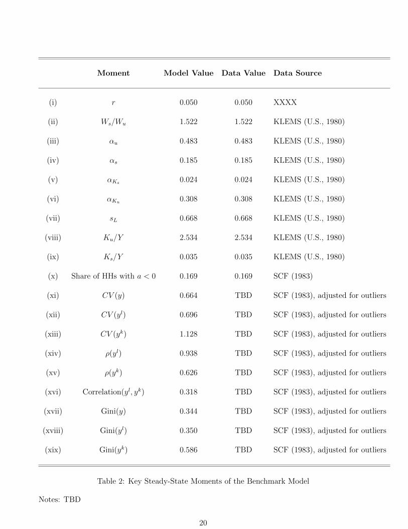
4.2 Characterizing the Stationary State
Key moments of the steady state of our model are listed in the first column of table 3. The
model’s values for the interest rate, skill-premium, factor shares, and share of borrowers in rows
(i) to (viii) are identical to the corresponding values in the data, as those moments were targets
used in our calibration strategy. (Ultimately, we’ll include CV (yl) in the exactly matched
category, but not here due to differences in CV and Gini.)
Figure 1 plots the distribution of capital income yk in the equilibrium of the economy.
Households each period experience changes in their particular asset holdings and capital income
but in steady state the distribution across these households is stationary. The vertical dashed
line to the left of zero corresponds to rψ < 0, the negative capital income associated with
interest payments on the largest amount of borrowing allowed. The total mass between that
dashed line and the zero value corresponds with the values in row (viii) of Table 3. Note that
there is essentially no mass at the borrowing constraint itself. Agents always respond at least
a bit to their precautionary saving motive given the potential for a negative shock in the next
period.
The modal capital income is below 0.5 in Figure 1, but there is significant mass to the right
of that point, with some households earning many multiples of that amount in capital income.
Row (xi) of Table 3 shows that capital income inequality in the benchmark model equals XXX,
only XXX lower than the empirical counterpart in the U.S. in the early 1980s. (Describe here
how we adjust data, i.e. subtracting outliers, etc.)
The equilibrium distribution of labor income yl in the economy reflects two factors. First,
there is a skill premium and workers differ in their skill endowments. Second, within any given
skill endowment, labor income varies with the AR1 process (36). Figure 2 plots the labor
distributions for each endowment type separately. The domain of both distributions includes
only positive labor incomes. The skilled distribution is shifted somewhat to the right of the
other distribution as the skill premium is positive. Given the AR1 process applies to the log
rather than the level of the labor endowment, this further results in more dispersion and greater
13

mass on very large incomes for the skilled distribution. As shown in Row (x) of Table 3, these
forces lead to overall labor income inequality in the benchmark model of XXX, which equals
that in the data as it was a targeted moment used in our calibration strategy.
[BN: I would like to add here a Figure with 3 lines – capital, labor, and total income. This
would allow us to discuss the intuition behind the ρ values, which we will list in the table. In
particular, if ρ(Y l, Y k) = 0, we’d expect the labor and capital lines to sort of “average” together
to form the overal income line. If ρ(Y l, Y k) > 0, these lines should both be more visually
concentrated than the total income. Now, our decomposition does not use ρ(Y l, Y k) = 0 (it
instead uses the related but different ρ(Y k, Y )), so I don’t know if this will work. But I’d like
to try. I believe John has a note saying this looks bad due to scaling or something, but it’d
help me to see the issue.]
5 Experiments
We now consider several experiments in which we introduce a shock which results in a new
stationary state of the system. We compare the initial and final stationary states to demonstrate
the repercussions of the shock for labor, capital, and overall inequality.
5.1 Changes in the Relative Price of Capital Goods
The first shock we consider decreases the price of IT investment, ξs, relative to that of non-IT
investment, ξu. (SOURCE) suggests that ξs/ξu declined by 50% from 1980 to 2010. ξs and
ξu are not identified in levels in the model, so we hold ξu = 1 and consider a decline in ξs
from 1 (the benchmark value) to 0.5. Key moments of the resulting steady state are listed in
the second column of 3. The changes to the capital, labor, and total income distributions are
plotted in figures 4, 5, and 6 respectively.
The IT rental rate Rs = ξs(r + δs) falls because the decline in ξs dominates any change
to the interest rate in equilibrium. The steady state value of Ks rises because it has become
cheaper, but not by enough to offset the rental rate decline, so the IT share αKs declines from
0.05 to 0.04.
14

IT capital and skilled labor are complements, so firms would like to hire more skilled workers
relative to unskilled workers. But, the supply of skilled and unskilled labor is fixed, so the wages
must adjust: the wage premium ws/wu rises from 1.50 to 1.59, and αs rises from 0.60 to 0.61.
Because the wage premium rises, labor income inequality also rises, with the coefficient
of variation growing from 0.70 to 0.72. Without any significant change to the precautionary
savings motive, capital income inequality rises just because households with higher labor income
save more, and labor income inequality has grown. The correlations ρ(yl) and ρ(yk) change
very little, so total income inequality increases too.
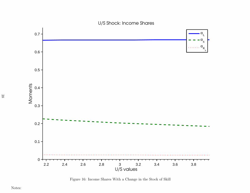
5.2 Changes in the Stock of Skill
The next shock increases the supply of skilled labor. Specifically, we reduce the ratio of un-
skilled to skilled labor U/S from 1.5 (the benchmark) to 1, the level suggested by (INSERT
SOURCE/MOTIVATION). Key moments of the resulting steady state are listed in the third
column of 3. The changes to the capital, labor, and total income distributions are plotted in
figures 11, 12, and 13 respectively.
The wage premium ws/wu declines from 1.5 to 1.19 because unskilled labor becomes scarcer
relative to skilled labor. Yet, the skilled labor share αS rises and and the unskilled labor share
αu falls; in the benchmark calibration skilled and unskilled labor are complementary, so the
wages do not move enough to offset the quantity changes. In sum, the labor share falls form
0.60 to 0.59. αKu is fixed by the Cobb-Douglas assumption, so it is αKs that increases. The
interest rate doesn’t move enough to significantly affect the rental rate of capital, because there
is little change to households’ precautionary savings motive, so the αKs increase is driven by
quantity. IT capital is complementary to skilled labor, which has increased, so firms substitute
towards IT capital. (NOTE: if we pick new elasticities, this may have to be rewritten)
All inequality moments exhibit large changes, and The decreased skill premium drives
changes to all five inequality moments. Labor income inequality falls because the skill pre-
mium has fallen (note the skilled/unskilled distributions in 12 shifting towards one another).
Capital income inequality falls directly because of the decreased labor income inequality - the
15

precautionary savings motive is mostly unaffected, so the relationship between household labor
income and their savings decision is also unaffected. The labor/total income correlation is
unchanged, but the capital/total income correlation falls. [I NEED INTUITION FOR THIS
ONE!]
5.3 Changes in Borrowing Limits
The final shock decreases the borrowing constraint, ψ, relative to that of non-IT investment,
xiu. We reduce the borrowing constraint from -1.08 to -10, which yields an increase in the share
of households with nonpositive wealth from 0.12 to 0.17, roughly the increase for 1980 to 2010,
measured by the Survey of Consumer Finances (NOTE: We should reproduce ourselves). Key
moments of the resulting steady state are listed in the fourth column of 3. The changes to the
capital, labor, and total income distributions are plotted in figures 18, 19, and 20 respectively.
When the borrowing constraint is relaxed, households have less incentive to hold assets as
precautionary savings, so the interest rate rises in equilibrium. The steady state capital stock
must be lower to produce the higher interest rate, but the price and quantity changes offset each
other offset each other (perfectly in the case of Ku), so the factor shares are largely unchanged.
Labor supplies are constant, so the wage premium doesn’t move very much either.
However, there are significant implications for inequality. With greater ability to borrow,
a larger share of households hold negative wealth in the stationary distribution. The greater
range of assets holdings also increases capital income inequality. Labor income inequality is
unchanged because skill allocations, wages, and the labor income process are unchanged. The
correlation between capital and total income rises because agents are able to adjust their wealth
more to self-insure as their labor income evolves. With improved self-insurance, the correlation
between labor and total income falls. However, this correlation decrease is dominated by the
increased capital income inequality in the decomposition of total income inequality (equation
1), so total income inequality increases.
16

6 Extensions
There are two goals of this section. The first is to convince the reader that our main conclusions
are robust to allowing for features that move us closer to the frontier. The second is to address
shortcomings of the basic model. For example, the basic model may underpredict capital
income inequality. So we will introduce heterogeneous discount factors to address this and
then ask how our conclusions are affected.
6.1 Heterogeneity in Discount Factors
6.2 Endogenous Labor Supply
6.3 Taxes and Transfers
6.4 Life-Cycle
Introduce a new dimension of heterogeneity, say q, that denotes stochastic movements across
different stages of the life-cycle. For example q could be young, middle aged and retired. Pick
transitions of q to match age profile of labor force. q should be correlated with z shocks to
mimic the hump shape in life-cycle wages. See e.g. Castaneda et al 2003, JPE.
7 Cross-Country Empirics, Shock Estimation, Quantita-
tive Results, Etc.
Clearly, all three of us would like to push in the empirical direction and speak more closely
with the data. We feel confident we’ll get there in at least some way, but we should completely
ignore this for now. Make the above sections tight and compelling, and this will work itself out
later.
8 Concluding Remarks
17

References
Aiyagari, R. (1994): “Uninsured Idiosyncratic Risk and Aggregate Saving,” The Quarterly
Journal of Economics, 109(3), 659–684.
Carroll, C. (2006): “The Method of Endogenous Gridpoints for Solving Dynamic Stochastic
Optimization Problems,” Economics Letters, 91(3), 312–320.
Guvenen, F. (2007): “Learning Your Earning: Are Labor Income Shocks Really Very Persis-
tent?,” American Economic Review, 97(3), 687–712.
Heathcote, J., K. Storesletten, and G. L. Violante (2010): “The Macroeconomic
Implications of Rising Wage Inequality in the United States,” Journal of Political Economy,
118(4), 681–722.
Huggett, M. (1996): “Wealth Distribution in Life-Cycle Economies,” Journal of Monetary
Economics, 38(3), 469–494.
Krusell, P., L. E. Ohanian, J.-V. Rios-Rull, and G. L. Violante (2000): “Capital-
Skill Complementarity and Inequality: A Macroeconomic Analysis,” Econometrica, 68(5),
1029–1053.
Shorrocks, A. (1982): “Inequality Decomposition by Factor Components,” Econometrica,
50(1), 193–211.
Tauchen, G. (1986): “Finite State Markov-chain Approximations to Univariate and Vector
Autoregressions,” Economics Letters, 20(2), 177–181.
18

Parameter AKN Value Cobb-Douglas Value Target Moment Target Source
Panel A: Externally Calibrated Parameters
(i) ρ 0.820 0.820 Guvenen (2007)
(ii) γ 1.500 1.500 Heathcote, Storesletten, and Violante (2010)
(iii) (εk, εs) (2.000, 1.500) (1.000, 1.000) XXXXXXX
(iv) (δu, δs) (0.037, 0.145) (0.037, 0.145) KLEMS (U.S., 1980)
(v) A 1.000 1.000 Normalization
Panel B: Internally Calibrated Parameters
(vi) σ2 0.129 0.129 Gini(yl) To Be Added (0.35 for now)
(vii) (φu, φs, φk) (0.308, 0.509, 0.216) (0.308, 0.302, 0.115) (αu, αs, αKu) KLEMS (U.S., 1980)
(viii) (ξu, ξs) (1.397, 3.517) (1.397, 3.517) (Ku/Y,Ks/Y ) KLEMS (U.S., 1980)
(ix) U/S 3.974 3.974 Ws/Wu KLEMS (U.S., 1980)
(x) ψ -0.683 -0.847 % of HHs with a < 0 SCF (1983)
(xi) β 0.937 0.937 r To Be Added
Table 1: Calibration of Model Parameters
Notes: TBD
19
Moment Model Value Data Value Data Source
(i) r 0.050 0.050 XXXX
(ii) Ws/Wu 1.522 1.522 KLEMS (U.S., 1980)
(iii) αu 0.483 0.483 KLEMS (U.S., 1980)
(iv) αs 0.185 0.185 KLEMS (U.S., 1980)
(v) αKs 0.024 0.024 KLEMS (U.S., 1980)
(vi) αKu 0.308 0.308 KLEMS (U.S., 1980)
(vii) sL 0.668 0.668 KLEMS (U.S., 1980)
(viii) Ku/Y 2.534 2.534 KLEMS (U.S., 1980)
(ix) Ks/Y 0.035 0.035 KLEMS (U.S., 1980)
(x) Share of HHs with a < 0 0.169 0.169 SCF (1983)
(xi) CV (y) 0.664 TBD SCF (1983), adjusted for outliers
(xii) CV (yl) 0.696 TBD SCF (1983), adjusted for outliers
(xiii) CV (yk) 1.128 TBD SCF (1983), adjusted for outliers
(xiv) ρ(yl) 0.938 TBD SCF (1983), adjusted for outliers
(xv) ρ(yk) 0.626 TBD SCF (1983), adjusted for outliers
(xvi) Correlation(yl, yk) 0.318 TBD SCF (1983), adjusted for outliers
(xvii) Gini(y) 0.344 TBD SCF (1983), adjusted for outliers
(xviii) Gini(yl) 0.350 TBD SCF (1983), adjusted for outliers
(xix) Gini(yk) 0.586 TBD SCF (1983), adjusted for outliers
Table 2: Key Steady-State Moments of the Benchmark Model
Notes: TBD
20

Moment Baseline Value ξs = 0.492 U/S = 2.18 ψ = −10 τc = 0.4
(i) r 0.050 0.052 0.050 0.052 0.053
(ii) Ws/Wu 1.522 1.682 1.122 1.521 1.493
(iii) αu 0.483 0.437 0.440 0.483 0.491
(iv) αs 0.185 0.185 0.226 0.185 0.185
(v) αKs 0.024 0.070 0.027 0.024 0.016
(vi) αKu 0.308 0.308 0.308 0.308 0.308
(vii) sL 0.668 0.622 0.666 0.668 0.676
(viii) Ku/Y 2.534 2.488 2.532 2.489 1.466
(ix) Ks/Y 0.035 0.726 0.038 0.034 0.014
(x) % of HHs with a < 0 0.169 0.139 0.163 0.244 0.244
(xi) CV (y) 0.664 0.678 0.627 0.677 0.681
(xii) CV (yl) 0.696 0.718 0.661 0.696 0.692
(xiii) CV (yk) 1.128 1.086 1.086 1.263 1.294
(xiv) ρ(yl) 0.938 0.931 0.933 0.921 0.921
(xv) ρ(yk) 0.626 0.650 0.610 0.636 0.650
(xvi) Correlation(yl, yk) 0.318 0.348 0.285 0.287 0.301
(xvii) Gini(y) 0.344 0.347 0.330 0.352 0.354
(xviii) Gini(yl) 0.350 0.357 0.338 0.350 0.349
(xix) Gini(yk) 0.586 0.560 0.574 0.667 0.669
Table 3: Key Steady-State Moments in Simulated Experiments - Baseline Specification
Notes: Experiment 1 reduces the price ξs of IT capital by 86%, from 3.517 to 0.492. Experiment2 reduces the ratio of unskilled to skilled labor by 45%, from 3.974 to 2.18. Experiment 3 reducesthe borrowing constraint ψ from -0.765 to -10. Experiment 4 increases the corporate income taxfrom 0 to 0.4. 21

Moment Baseline Value ξs = 0.492 U/S = 2.18 ψ = −10
(i) r 0.050 0.050 0.050 0.052
(ii) Ws/Wu 1.522 1.522 0.837 1.522
(iii) αu 0.483 0.483 0.483 0.483
(iv) αs 0.185 0.185 0.185 0.185
(v) αKs 0.024 0.024 0.024 0.024
(vi) αKu 0.308 0.308 0.308 0.308
(vii) sL 0.668 0.668 0.668 0.668
(viii) Ku/Y 2.534 2.534 2.534 2.487
(ix) Ks/Y 0.035 0.250 0.035 0.035
(x) % of HHs with a < 0 0.169 0.163 0.167 0.237
(xi) CV (y) 0.664 0.664 0.632 0.676
(xii) CV (yl) 0.696 0.696 0.665 0.696
(xiii) CV (yk) 1.128 1.120 1.096 1.255
(xiv) ρ(yl) 0.938 0.939 0.934 0.922
(xv) ρ(yk) 0.627 0.625 0.612 0.636
(xvi) Correlation(yl, yk) 0.318 0.319 0.288 0.288
(xvii) Gini(y) 0.344 0.343 0.332 0.351
(xviii) Gini(yl) 0.350 0.350 0.339 0.350
(xix) Gini(yk) 0.587 0.582 0.578 0.662
Table 4: Key Steady-State Moments in Simulated Experiments - Cobb-Douglas Specification
Notes: Experiment 1 reduces the price ξs of IT capital by 86%, from 3.517 to 0.492. Experiment2 reduces the ratio of unskilled to skilled labor by 45%, from 3.974 to 2.18. Experiment 3 reducesthe borrowing constraint ψ from -0.765 to -10.
22

−1 −0.5 0 0.5 1 1.5 2 2.5 3 3.5 40
0.5
1
1.5
2
2.5
3
Asset Income
Ho
use
ho
lds
Asset Income Distribution
HouseholdsBorrowing Constraint
Figure 1: Benchmark Capital Income Distribution
Notes:
23

0 0.5 1 1.5 2 2.5 30
0.5
1
1.5
Labor Income
Wo
rke
rs
Labor Income by Type
Low SkillHigh Skill
Figure 2: Benchmark Labor Income Distribution by Skill Type
Notes:
24

0 1 2 3 4 5 6 7 8 9 100
0.2
0.4
0.6
0.8
1
1.2
Household Income
Ma
ss
Total Income Distribution
Figure 3: Benchmark Total Income Distribution
Notes:
25

−1 −0.5 0 0.5 1 1.5 2 2.5 3 3.5 40
0.5
1
1.5
2
2.5
3
Asset Income
Ho
use
ho
lds
ξS Shock: Asset Income Distribution
xis = 0.49231 Householdsxis = 3.5165 HouseholdsBorrowing Constraint
Figure 4: Capital Income Distribution With an IT Price Shock
Notes:
26

0 0.5 1 1.5 2 2.5 3 3.50
0.5
1
1.5
Labor Income
Ho
use
ho
lds
ξS Shock: Labor Income by Type
ξ
S = 0.49231 Low Skill
ξS = 0.49231 High Skill
ξS = 3.5165 Low Skill
ξS = 3.5165 High Skill
Figure 5: Benchmark Labor Income Distribution by Skill Type With an IT Price Shock
Notes:
27

0 1 2 3 4 5 6 7 8 9 100
0.2
0.4
0.6
0.8
1
1.2
Household Income
Ho
use
ho
lds
ξS Shock: Total Income Distribution
ξ
S = 0.49231 Households
ξS = 3.5165 Households
Figure 6: Total Income Distribution With an IT Price Shock
Notes:
28

0.5 1 1.5 2 2.5 3 3.50
0.2
0.4
0.6
0.8
1
1.2
ξS values
Mo
me
nts
ξS Shock: Coefficients of Variation
CV Total IncomeCV Labor IncomeCV Asset Income
Figure 7: Coefficients of Variation With an IT Price Shock
Notes:
29

0.5 1 1.5 2 2.5 3 3.50
0.1
0.2
0.3
0.4
0.5
0.6
0.7
0.8
0.9
1
ξS values
Mo
me
nts
ξS Shock: Correlations
ρy,l
ρy,k
ρl,k
Figure 8: Correlations With an IT Price Shock
Notes:
30

0.5 1 1.5 2 2.5 3 3.50
0.1
0.2
0.3
0.4
0.5
0.6
0.7
ξS values
Mo
me
nts
ξS Shock: Income Shares
α
L
αs
αK
s
Figure 9: Income Shares With an IT Price Shock
Notes:
31

0.5 1 1.5 2 2.5 3 3.50
0.5
1
1.5
2
2.5
3
3.5
ξS values
Mo
me
nts
ξS Shock: Capital Moments
Interest Rateξ
u*K
u/Y
ξs*K
s/Y
Figure 10: Capital Moments With an IT Price Shock
Notes:
32

−1 −0.5 0 0.5 1 1.5 2 2.5 3 3.5 40
0.5
1
1.5
2
2.5
3
Asset Income
Ho
use
ho
lds
U/S Shock: Asset Income Distribution
USratio = 2.16 HouseholdsUSratio = 3.9737 HouseholdsBorrowing Constraint
Figure 11: Benchmark Capital Income Distribution With a Change in the Stock of Skill
Notes:
33

0 0.5 1 1.5 2 2.5 30
0.5
1
1.5
Labor Income
Ho
use
ho
lds
U/S Shock: Labor Income by Type
U/S = 2.16 Low SkillU/S = 2.16 High SkillU/S = 3.9737 Low SkillU/S = 3.9737 High Skill
Figure 12: Benchmark Labor Income Distribution by Skill Type With a Change in the Stock of Skill
Notes:
34

0 1 2 3 4 5 6 7 8 9 100
0.2
0.4
0.6
0.8
1
1.2
Household Income
Ho
use
ho
lds
U/S Shock: Total Income Distribution
U/S = 2.16 HouseholdsU/S = 3.9737 Households
Figure 13: Total Income Distribution With a Change in the Stock of Skill
Notes:
35

2.2 2.4 2.6 2.8 3 3.2 3.4 3.6 3.80
0.2
0.4
0.6
0.8
1
1.2
U/S values
Mo
me
nts
U/S Shock: Coefficients of Variation
CV Total IncomeCV Labor IncomeCV Asset Income
Figure 14: Coefficients of Variation With a Change in the Stock of Skill
Notes:
36

2.2 2.4 2.6 2.8 3 3.2 3.4 3.6 3.80
0.1
0.2
0.3
0.4
0.5
0.6
0.7
0.8
0.9
1
U/S values
Mo
me
nts
U/S Shock: Correlations
ρy,l
ρy,k
ρl,k
Figure 15: Correlations With a Change in the Stock of Skill
Notes:
37
2.2 2.4 2.6 2.8 3 3.2 3.4 3.6 3.80
0.1
0.2
0.3
0.4
0.5
0.6
0.7
U/S values
Mo
me
nts
U/S Shock: Income Shares
α
L
αs
αK
s
Figure 16: Income Shares With a Change in the Stock of Skill
Notes:
38

2.2 2.4 2.6 2.8 3 3.2 3.4 3.6 3.80
0.5
1
1.5
2
2.5
3
3.5
U/S values
Mo
me
nts
U/S Shock: Capital Moments
Interest Rateξ
u*K
u/Y
ξs*K
s/Y
Figure 17: Capital Moments With a Change in the Stock of Skill
Notes:
39

−1 −0.5 0 0.5 1 1.5 2 2.5 3 3.5 40
0.5
1
1.5
2
2.5
3
Asset Income
Ho
use
ho
lds
ψ Shock: Asset Income Distribution
ψ = −10 Householdsψ = −0.6825 Householdsψ = −10 Borrowing Constraintψ = −0.6825 Borrowing Constraint
Figure 18: Benchmark Capital Income Distribution With a Change in the Borrowing Constraint
Notes:
40

0 0.5 1 1.5 2 2.5 30
0.5
1
1.5
Labor Income
Ho
use
ho
lds
ψ Shock: Labor Income by Type
ψ = −10 Low Skillψ = −10 High Skillψ = −0.6825 Low Skillψ = −0.6825 High Skill
Figure 19: Benchmark Labor Income Distribution by Skill Type With a Change in the Borrowing Constraint
Notes:
41

0 1 2 3 4 5 6 7 8 9 100
0.2
0.4
0.6
0.8
1
1.2
1.4
Household Income
Ho
use
ho
lds
ψ Shock: Total Income Distribution
ψ = −10 Householdsψ = −0.6825 Households
Figure 20: Total Income Distribution With a Change in the Borrowing Constraint
Notes:
42

−10 −9 −8 −7 −6 −5 −4 −3 −2 −10
0.2
0.4
0.6
0.8
1
1.2
1.4
ψ values
Mo
me
nts
ψ Shock: Coefficients of Variation
CV Total IncomeCV Labor IncomeCV Asset Income
Figure 21: Coefficients of Variation With a Change in the Borrowing Constraint
Notes:
43

−10 −9 −8 −7 −6 −5 −4 −3 −2 −10
0.1
0.2
0.3
0.4
0.5
0.6
0.7
0.8
0.9
1
ψ values
Mo
me
nts
ψ Shock: Correlations
ρy,l
ρy,k
ρl,k
Figure 22: Correlations With a Change in the Borrowing Constraint
Notes:
44

−10 −9 −8 −7 −6 −5 −4 −3 −2 −10
0.1
0.2
0.3
0.4
0.5
0.6
0.7
ψ values
Mo
me
nts
ψ Shock: Income Shares
α
L
αs
αK
s
Figure 23: Income Shares With a Change in the Borrowing Constraint
Notes:
45

−10 −9 −8 −7 −6 −5 −4 −3 −2 −10
0.5
1
1.5
2
2.5
3
3.5
ψ values
Mo
me
nts
ψ Shock: Capital Moments
Interest Rateξ
u*K
u/Y
ξs*K
s/Y
Figure 24: Capital Moments With a Change in the Borrowing Constraint
Notes:
46

−1 −0.5 0 0.5 1 1.5 2 2.5 3 3.5 40
0.5
1
1.5
2
2.5
3
Asset Income
Ho
use
ho
lds
τK Shock: Asset Income Distribution
tauk = 0 Householdstauk = 0.4 HouseholdsBorrowing Constraint
Figure 25: Benchmark Capital Income Distribution With a Change in the Capital Tax
Notes:
47

0 0.5 1 1.5 2 2.5 30
0.5
1
1.5
Labor Income
Ho
use
ho
lds
τK Shock: Labor Income by Type
τK = 0 Low Skill
τK = 0 High Skill
τK = 0.4 Low Skill
τK = 0.4 High Skill
Figure 26: Benchmark Labor Income Distribution by Skill Type With a Change in the Capital Tax
Notes:
48

0 1 2 3 4 5 6 7 8 9 100
0.2
0.4
0.6
0.8
1
1.2
Household Income
Ho
use
ho
lds
τK Shock: Total Income Distribution
τK = 0 Households
τK = 0.4 Households
Figure 27: Total Income Distribution With a Change in the Capital Tax
Notes:
49

0 0.05 0.1 0.15 0.2 0.25 0.3 0.35 0.40
0.2
0.4
0.6
0.8
1
1.2
τK values
Mo
me
nts
τK Shock: Coefficients of Variation
CV Total IncomeCV Labor IncomeCV Asset Income
Figure 28: Coefficients of Variation With a Change in the Capital Tax
Notes:
50

0 0.05 0.1 0.15 0.2 0.25 0.3 0.35 0.40
0.1
0.2
0.3
0.4
0.5
0.6
0.7
0.8
0.9
1
τK values
Mo
me
nts
τK Shock: Correlations
ρy,l
ρy,k
ρl,k
Figure 29: Correlations With a Change in the Capital Tax
Notes:
51
0 0.05 0.1 0.15 0.2 0.25 0.3 0.35 0.40
0.1
0.2
0.3
0.4
0.5
0.6
0.7
τK values
Mo
me
nts
τK Shock: Income Shares
α
L
αs
αK
s
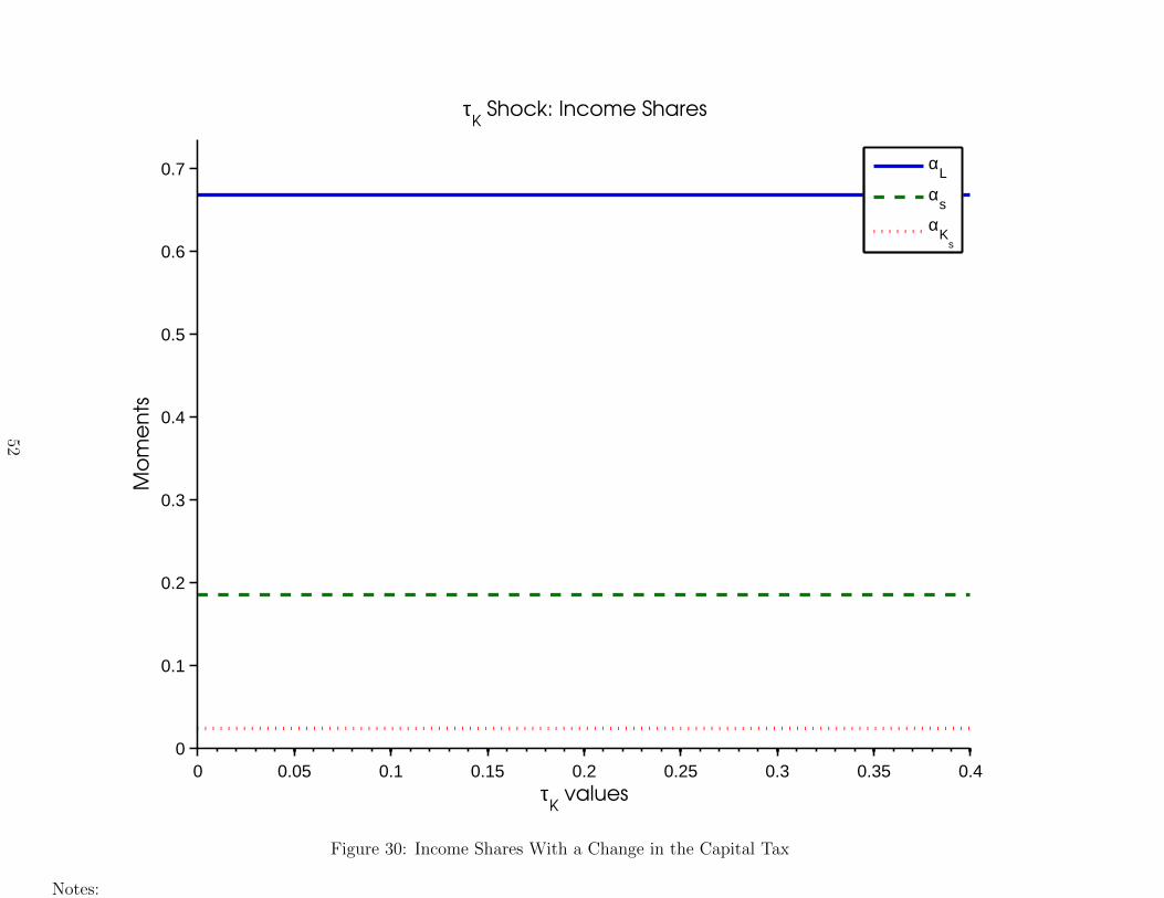
Figure 30: Income Shares With a Change in the Capital Tax
Notes:
52

0 0.05 0.1 0.15 0.2 0.25 0.3 0.35 0.40
0.5
1
1.5
2
2.5
3
3.5
τK values
Mo
me
nts
τK Shock: Capital Moments
Interest Rateξ
u*K
u/Y
ξs*K
s/Y
Figure 31: Capital Moments With a Change in the Capital Tax
Notes:
53

−1 −0.5 0 0.5 1 1.5 2 2.5 3 3.5 40
0.5
1
1.5
2
2.5
3
3.5
Asset Income
Ho
use
ho
lds
τC
Shock: Asset Income Distribution
tauc = 0 Householdstauc = 0.4 HouseholdsBorrowing Constraint
Figure 32: Benchmark Capital Income Distribution With a Change in the Corporate Tax
Notes:
54

0 0.5 1 1.5 2 2.5 30
0.2
0.4
0.6
0.8
1
1.2
1.4
1.6
1.8
2
Labor Income
Ho
use
ho
lds
τC
Shock: Labor Income by Type
τC
= 0 Low Skill
τC
= 0 High Skill
τC
= 0.4 Low Skill
τC
= 0.4 High Skill
Figure 33: Benchmark Labor Income Distribution by Skill Type With a Change in the Corporate Tax
Notes:
55

0 1 2 3 4 5 6 7 8 9 100
0.2
0.4
0.6
0.8
1
1.2
1.4
1.6
Household Income
Ho
use
ho
lds
τC
Shock: Total Income Distribution
τC
= 0 Households
τC
= 0.4 Households
Figure 34: Total Income Distribution With a Change in the Corporate Tax
Notes:
56

0 0.05 0.1 0.15 0.2 0.25 0.3 0.35 0.40
0.2
0.4
0.6
0.8
1
1.2
1.4
τC
values
Mo
me
nts
τC
Shock: Coefficients of Variation
CV Total IncomeCV Labor IncomeCV Asset Income
Figure 35: Coefficients of Variation With a Change in the Corporate Tax
Notes:
57

0 0.05 0.1 0.15 0.2 0.25 0.3 0.35 0.40
0.1
0.2
0.3
0.4
0.5
0.6
0.7
0.8
0.9
1
τC
values
Mo
me
nts
τC
Shock: Correlations
ρy,l
ρy,k
ρl,k
Figure 36: Correlations With a Change in the Corporate Tax
Notes:
58

0 0.05 0.1 0.15 0.2 0.25 0.3 0.35 0.40
0.1
0.2
0.3
0.4
0.5
0.6
0.7
τC
values
Mo
me
nts
τC
Shock: Income Shares
α
L
αs
αK
s
Figure 37: Income Shares With a Change in the Corporate Tax
Notes:
59
0 0.05 0.1 0.15 0.2 0.25 0.3 0.35 0.40
0.5
1
1.5
2
2.5
3
3.5
τC
values
Mo
me
nts
τC
Shock: Capital Moments
Interest Rateξ
u*K
u/Y
ξs*K
s/Y
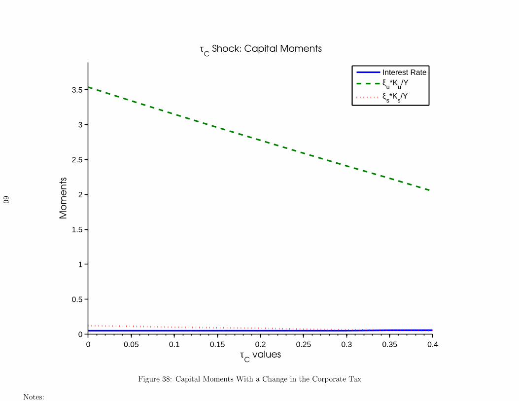
Figure 38: Capital Moments With a Change in the Corporate Tax
Notes:
60

−1 −0.5 0 0.5 1 1.5 2 2.5 3 3.5 40
0.5
1
1.5
2
2.5
3
Asset Income
Ho
use
ho
lds
σ Shock: Asset Income Distribution
sigma = 0.3589 Householdssigma = 0.53835 HouseholdsBorrowing Constraint
Figure 39: Benchmark Capital Income Distribution With a Change in the Labor Income Variance
Notes:
61

0 0.5 1 1.5 2 2.5 30
0.5
1
1.5
Labor Income
Ho
use
ho
lds
σ Shock: Labor Income by Type
σ = 0.3589 Low Skillσ = 0.3589 High Skillσ = 0.53835 Low Skillσ = 0.53835 High Skill
Figure 40: Benchmark Labor Income Distribution by Skill Type With a Change in the Labor Income Variance
Notes:
62

0 1 2 3 4 5 6 7 8 9 100
0.2
0.4
0.6
0.8
1
1.2
Household Income
Ho
use
ho
lds
σ Shock: Total Income Distribution
σ = 0.3589 Householdsσ = 0.53835 Households
Figure 41: Total Income Distribution With a Change in the Labor Income Variance
Notes:
63

0.36 0.38 0.4 0.42 0.44 0.46 0.48 0.5 0.520
0.2
0.4
0.6
0.8
1
1.2
σ values
Mo
me
nts
σ Shock: Coefficients of Variation
CV Total IncomeCV Labor IncomeCV Asset Income
Figure 42: Coefficients of Variation With a Change in the Labor Income Variance
Notes:
64

0.36 0.38 0.4 0.42 0.44 0.46 0.48 0.5 0.520
0.1
0.2
0.3
0.4
0.5
0.6
0.7
0.8
0.9
1
σ values
Mo
me
nts
σ Shock: Correlations
ρy,l
ρy,k
ρl,k
Figure 43: Correlations With a Change in the Labor Income Variance
Notes:
65

0.36 0.38 0.4 0.42 0.44 0.46 0.48 0.5 0.520
0.1
0.2
0.3
0.4
0.5
0.6
0.7
σ values
Mo
me
nts
σ Shock: Income Shares
α
L
αs
αK
s
Figure 44: Income Shares With a Change in the Labor Income Variance
Notes:
66

0.36 0.38 0.4 0.42 0.44 0.46 0.48 0.5 0.520
0.5
1
1.5
2
2.5
3
3.5
4
4.5
σ values
Mo
me
nts
σ Shock: Capital Moments
Interest Rateξ
u*K
u/Y
ξs*K
s/Y
Figure 45: Capital Moments With a Change in the Labor Income Variance
Notes:
67

−1 −0.5 0 0.5 1 1.5 2 2.5 3 3.5 40
0.5
1
1.5
2
2.5
3
3.5
Asset Income
Ho
use
ho
lds
ρ Shock: Asset Income Distribution
rho = 0.6 Householdsrho = 0.95 HouseholdsBorrowing Constraint
Figure 46: Benchmark Capital Income Distribution With a Change in the Labor Income Persistence
Notes:
68

0 0.5 1 1.5 2 2.5 3 3.50
0.2
0.4
0.6
0.8
1
1.2
1.4
1.6
Labor Income
Ho
use
ho
lds
ρ Shock: Labor Income by Type
ρ = 0.6 Low Skillρ = 0.6 High Skillρ = 0.95 Low Skillρ = 0.95 High Skill
Figure 47: Benchmark Labor Income Distribution by Skill Type With a Change in the Labor Income Persistence
Notes:
69

0 1 2 3 4 5 6 7 8 9 100
0.2
0.4
0.6
0.8
1
1.2
1.4
1.6
1.8
Household Income
Ho
use
ho
lds
ρ Shock: Total Income Distribution
ρ = 0.6 Householdsρ = 0.95 Households
Figure 48: Total Income Distribution With a Change in the Labor Income Persistence
Notes:
70

0.6 0.65 0.7 0.75 0.8 0.85 0.90
0.2
0.4
0.6
0.8
1
1.2
1.4
1.6
ρ values
Mo
me
nts
ρ Shock: Coefficients of Variation
CV Total IncomeCV Labor IncomeCV Asset Income
Figure 49: Coefficients of Variation With a Change in the Labor Income Persistence
Notes:
71

0.6 0.65 0.7 0.75 0.8 0.85 0.90
0.1
0.2
0.3
0.4
0.5
0.6
0.7
0.8
0.9
1
ρ values
Mo
me
nts
ρ Shock: Correlations
ρy,l
ρy,k
ρl,k
Figure 50: Correlations With a Change in the Labor Income Persistence
Notes:
72

0.6 0.65 0.7 0.75 0.8 0.85 0.90
0.1
0.2
0.3
0.4
0.5
0.6
0.7
ρ values
Mo
me
nts
ρ Shock: Income Shares
α
L
αs
αK
s
Figure 51: Income Shares With a Change in the Labor Income Persistence
Notes:
73

0.6 0.65 0.7 0.75 0.8 0.85 0.90
0.5
1
1.5
2
2.5
3
3.5
4
4.5
5
ρ values
Mo
me
nts
ρ Shock: Capital Moments
Interest Rateξ
u*K
u/Y
ξs*K
s/Y
Figure 52: Capital Moments With a Change in the Labor Income Persistence
Notes:
74
−1 −0.5 0 0.5 1 1.5 2 2.5 3 3.5 40
0.5
1
1.5
2
2.5
3
Asset Income
Ho
use
ho
lds
φU Shock: Asset Income Distribution
phiu = 0.308 Householdsphiu = 0.35 HouseholdsBorrowing Constraint
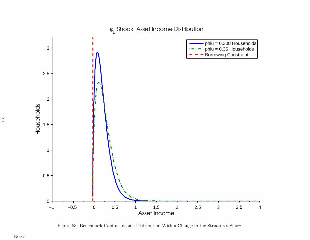
Figure 53: Benchmark Capital Income Distribution With a Change in the Structures Share
Notes:
75

0 0.5 1 1.5 2 2.5 30
0.5
1
1.5
Labor Income
Ho
use
ho
lds
φU Shock: Labor Income by Type
φ
U = 0.308 Low Skill
φU
= 0.308 High Skill
φU
= 0.35 Low Skill
φU
= 0.35 High Skill
Figure 54: Benchmark Labor Income Distribution by Skill Type With a Change in the Structures Share
Notes:
76

0 1 2 3 4 5 6 7 8 9 100
0.2
0.4
0.6
0.8
1
1.2
Household Income
Ho
use
ho
lds
φU Shock: Total Income Distribution
φ
U = 0.308 Households
φU
= 0.35 Households
Figure 55: Total Income Distribution With a Change in the Structures Share
Notes:
77
0.31 0.315 0.32 0.325 0.33 0.335 0.34 0.345 0.350
0.2
0.4
0.6
0.8
1
1.2
φU values
Mo
me
nts
φU Shock: Coefficients of Variation
CV Total IncomeCV Labor IncomeCV Asset Income
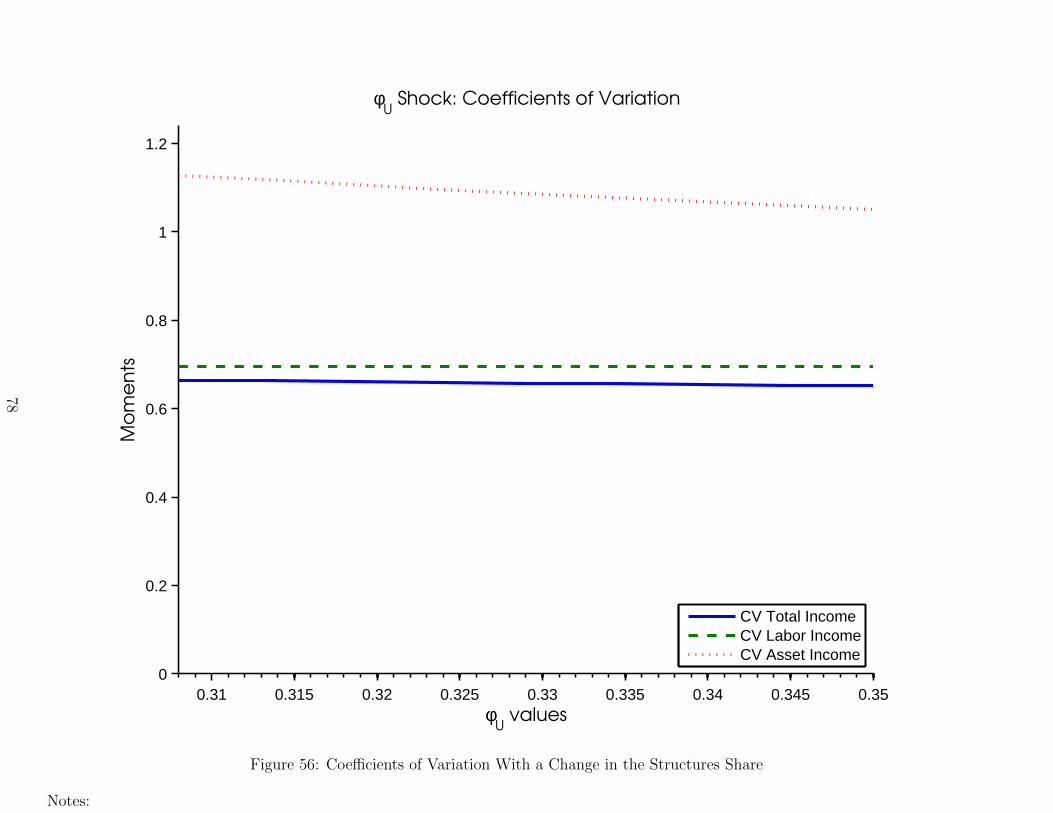
Figure 56: Coefficients of Variation With a Change in the Structures Share
Notes:
78

0.31 0.315 0.32 0.325 0.33 0.335 0.34 0.345 0.350
0.1
0.2
0.3
0.4
0.5
0.6
0.7
0.8
0.9
1
φU values
Mo
me
nts
φU Shock: Correlations
ρy,l
ρy,k
ρl,k
Figure 57: Correlations With a Change in the Structures Share
Notes:
79

0.31 0.315 0.32 0.325 0.33 0.335 0.34 0.345 0.350
0.1
0.2
0.3
0.4
0.5
0.6
0.7
φU values
Mo
me
nts
φU Shock: Income Shares
α
L
αs
αK
s
Figure 58: Income Shares With a Change in the Structures Share
Notes:
80
0.31 0.315 0.32 0.325 0.33 0.335 0.34 0.345 0.350
0.5
1
1.5
2
2.5
3
3.5
4
φU values
Mo
me
nts
φU Shock: Capital Moments
Interest Rateξ
u*K
u/Y
ξs*K
s/Y
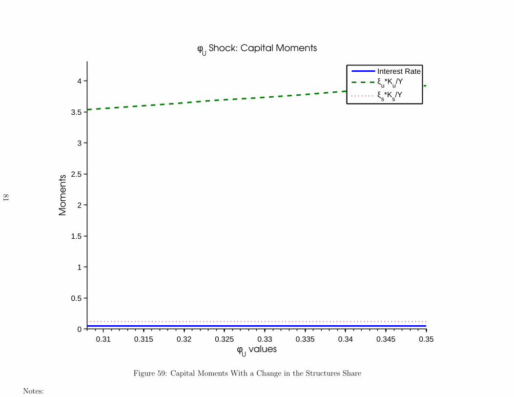
Figure 59: Capital Moments With a Change in the Structures Share
Notes:
81

−1 −0.5 0 0.5 1 1.5 2 2.5 3 3.5 40
0.5
1
1.5
2
2.5
Asset Income
Ho
use
ho
lds
Asset Income Distribution
HouseholdsBorrowing Constraint
Figure 60: Cobb-Douglas Capital Income Distribution
Notes:
82

0 0.5 1 1.5 2 2.5 3 3.50
0.2
0.4
0.6
0.8
1
1.2
1.4
Labor Income
Wo
rke
rs
Labor Income by Type
Low SkillHigh Skill
Figure 61: Cobb-Douglas Labor Income Distribution by Skill Type
Notes:
83

0 1 2 3 4 5 6 7 8 9 100
0.1
0.2
0.3
0.4
0.5
0.6
0.7
0.8
0.9
1
Household Income
Ma
ss
Total Income Distribution
Figure 62: Cobb-Douglas Total Income Distribution
Notes:
84

−1 −0.5 0 0.5 1 1.5 2 2.5 3 3.5 40
0.5
1
1.5
2
2.5
Asset Income
Ho
use
ho
lds
ξS Shock: Asset Income Distribution
xis = 0.49231 Householdsxis = 3.5165 HouseholdsBorrowing Constraint
Figure 63: Cobb-Douglas Capital Income Distribution With an IT Price Shock
Notes:
85

0 0.5 1 1.5 2 2.5 3 3.5 40
0.2
0.4
0.6
0.8
1
1.2
1.4
Labor Income
Ho
use
ho
lds
ξS Shock: Labor Income by Type
ξ
S = 0.49231 Low Skill
ξS = 0.49231 High Skill
ξS = 3.5165 Low Skill
ξS = 3.5165 High Skill
Figure 64: Cobb-Douglas Labor Income Distribution by Skill Type With an IT Price Shock
Notes:
86

0 1 2 3 4 5 6 7 8 9 100
0.1
0.2
0.3
0.4
0.5
0.6
0.7
0.8
0.9
1
Household Income
Ho
use
ho
lds
ξS Shock: Total Income Distribution
ξ
S = 0.49231 Households
ξS = 3.5165 Households
Figure 65: Cobb-Douglas Total Income Distribution With an IT Price Shock
Notes:
87

0.5 1 1.5 2 2.5 3 3.50
0.2
0.4
0.6
0.8
1
1.2
ξS values
Mo
me
nts
ξS Shock: Coefficients of Variation
CV Total IncomeCV Labor IncomeCV Asset Income
Figure 66: Cobb-Douglas Coefficients of Variation With an IT Price Shock
Notes:
88

0.5 1 1.5 2 2.5 3 3.50
0.1
0.2
0.3
0.4
0.5
0.6
0.7
0.8
0.9
1
ξS values
Mo
me
nts
ξS Shock: Correlations
ρy,l
ρy,k
ρl,k
Figure 67: Cobb-Douglas Correlations With an IT Price Shock
Notes:
89

0.5 1 1.5 2 2.5 3 3.50
0.1
0.2
0.3
0.4
0.5
0.6
0.7
ξS values
Mo
me
nts
ξS Shock: Income Shares
α
L
αs
αK
s
Figure 68: Cobb-Douglas Income Shares With an IT Price Shock
Notes:
90

0.5 1 1.5 2 2.5 3 3.50
0.5
1
1.5
2
2.5
3
3.5
ξS values
Mo
me
nts
ξS Shock: Capital Moments
Interest Rateξ
u*K
u/Y
ξs*K
s/Y
Figure 69: Cobb-Douglas Capital Moments With an IT Price Shock
Notes:
91

−1 −0.5 0 0.5 1 1.5 2 2.5 3 3.5 40
0.5
1
1.5
2
2.5
Asset Income
Ho
use
ho
lds
U/S Shock: Asset Income Distribution
USratio = 2.1855 HouseholdsUSratio = 3.9737 HouseholdsBorrowing Constraint
Figure 70: Cobb-Douglas Capital Income Distribution With a Change in the Stock of Skill
Notes:
92

0 0.5 1 1.5 2 2.5 3 3.50
0.2
0.4
0.6
0.8
1
1.2
1.4
Labor Income
Ho
use
ho
lds
U/S Shock: Labor Income by Type
U/S = 2.1855 Low SkillU/S = 2.1855 High SkillU/S = 3.9737 Low SkillU/S = 3.9737 High Skill
Figure 71: Cobb-Douglas Labor Income Distribution by Skill Type With a Change in the Stock of Skill
Notes:
93

0 1 2 3 4 5 6 7 8 9 100
0.1
0.2
0.3
0.4
0.5
0.6
0.7
0.8
0.9
1
Household Income
Ho
use
ho
lds
U/S Shock: Total Income Distribution
U/S = 2.1855 HouseholdsU/S = 3.9737 Households
Figure 72: Cobb-Douglas Total Income Distribution With a Change in the Stock of Skill
Notes:
94

2.2 2.4 2.6 2.8 3 3.2 3.4 3.6 3.80
0.2
0.4
0.6
0.8
1
1.2
U/S values
Mo
me
nts
U/S Shock: Coefficients of Variation
CV Total IncomeCV Labor IncomeCV Asset Income
Figure 73: Cobb-Douglas Coefficients of Variation With a Change in the Stock of Skill
Notes:
95

2.2 2.4 2.6 2.8 3 3.2 3.4 3.6 3.80
0.1
0.2
0.3
0.4
0.5
0.6
0.7
0.8
0.9
1
U/S values
Mo
me
nts
U/S Shock: Correlations
ρy,l
ρy,k
ρl,k
Figure 74: Cobb-Douglas Correlations With a Change in the Stock of Skill
Notes:
96

2.2 2.4 2.6 2.8 3 3.2 3.4 3.6 3.80
0.1
0.2
0.3
0.4
0.5
0.6
0.7
U/S values
Mo
me
nts
U/S Shock: Income Shares
α
L
αs
αK
s
Figure 75: Cobb-Douglas Income Shares With a Change in the Stock of Skill
Notes:
97

2.2 2.4 2.6 2.8 3 3.2 3.4 3.6 3.80
0.5
1
1.5
2
2.5
3
3.5
U/S values
Mo
me
nts
U/S Shock: Capital Moments
Interest Rateξ
u*K
u/Y
ξs*K
s/Y
Figure 76: Cobb-Douglas Capital Moments With a Change in the Stock of Skill
Notes:
98

−1 −0.5 0 0.5 1 1.5 2 2.5 3 3.5 40
0.5
1
1.5
2
2.5
Asset Income
Ho
use
ho
lds
ψ Shock: Asset Income Distribution
ψ = −10 Householdsψ = −0.847 Householdsψ = −10 Borrowing Constraintψ = −0.847 Borrowing Constraint
Figure 77: Cobb-Douglas Capital Income Distribution With a Change in the Borrowing Constraint
Notes:
99

0 0.5 1 1.5 2 2.5 3 3.50
0.2
0.4
0.6
0.8
1
1.2
1.4
Labor Income
Ho
use
ho
lds
ψ Shock: Labor Income by Type
ψ = −10 Low Skillψ = −10 High Skillψ = −0.847 Low Skillψ = −0.847 High Skill
Figure 78: Cobb-Douglas Labor Income Distribution by Skill Type With a Change in the Borrowing Constraint
Notes:
100

0 1 2 3 4 5 6 7 8 9 100
0.2
0.4
0.6
0.8
1
Household Income
Ho
use
ho
lds
ψ Shock: Total Income Distribution
ψ = −10 Householdsψ = −0.847 Households
Figure 79: Cobb-Douglas Total Income Distribution With a Change in the Borrowing Constraint
Notes:
101

−10 −9 −8 −7 −6 −5 −4 −3 −2 −10
0.2
0.4
0.6
0.8
1
1.2
1.4
ψ values
Mo
me
nts
ψ Shock: Coefficients of Variation
CV Total IncomeCV Labor IncomeCV Asset Income
Figure 80: Cobb-Douglas Coefficients of Variation With a Change in the Borrowing Constraint
Notes:
102

−10 −9 −8 −7 −6 −5 −4 −3 −2 −10
0.1
0.2
0.3
0.4
0.5
0.6
0.7
0.8
0.9
1
ψ values
Mo
me
nts
ψ Shock: Correlations
ρy,l
ρy,k
ρl,k
Figure 81: Cobb-Douglas Correlations With a Change in the Borrowing Constraint
Notes:
103

−10 −9 −8 −7 −6 −5 −4 −3 −2 −10
0.1
0.2
0.3
0.4
0.5
0.6
0.7
ψ values
Mo
me
nts
ψ Shock: Income Shares
α
L
αs
αK
s
Figure 82: Cobb-Douglas Income Shares With a Change in the Borrowing Constraint
Notes:
104

−10 −9 −8 −7 −6 −5 −4 −3 −2 −10
0.5
1
1.5
2
2.5
3
3.5
ψ values
Mo
me
nts
ψ Shock: Capital Moments
Interest Rateξ
u*K
u/Y
ξs*K
s/Y
Figure 83: Cobb-Douglas Capital Moments With a Change in the Borrowing Constraint
Notes:
105

−1 −0.5 0 0.5 1 1.5 2 2.5 3 3.5 40
0.5
1
1.5
2
2.5
Asset Income
Ho
use
ho
lds
σ Shock: Asset Income Distribution
sigma = 0.3589 Householdssigma = 0.53835 HouseholdsBorrowing Constraint
Figure 84: Cobb-Douglas Capital Income Distribution With a Change in the Labor Income Variance
Notes:
106

0 0.5 1 1.5 2 2.5 3 3.5 40
0.2
0.4
0.6
0.8
1
1.2
1.4
Labor Income
Ho
use
ho
lds
σ Shock: Labor Income by Type
σ = 0.3589 Low Skillσ = 0.3589 High Skillσ = 0.53835 Low Skillσ = 0.53835 High Skill
Figure 85: Cobb-Douglas Labor Income Distribution by Skill Type With a Change in the Labor Income Variance
Notes:
107

0 1 2 3 4 5 6 7 8 9 100
0.1
0.2
0.3
0.4
0.5
0.6
0.7
0.8
0.9
1
Household Income
Ho
use
ho
lds
σ Shock: Total Income Distribution
σ = 0.3589 Householdsσ = 0.53835 Households
Figure 86: Cobb-Douglas Total Income Distribution With a Change in the Labor Income Variance
Notes:
108

0.36 0.38 0.4 0.42 0.44 0.46 0.48 0.5 0.520
0.2
0.4
0.6
0.8
1
1.2
σ values
Mo
me
nts
σ Shock: Coefficients of Variation
CV Total IncomeCV Labor IncomeCV Asset Income
Figure 87: Cobb-Douglas Coefficients of Variation With a Change in the Labor Income Variance
Notes:
109

0.36 0.38 0.4 0.42 0.44 0.46 0.48 0.5 0.520
0.1
0.2
0.3
0.4
0.5
0.6
0.7
0.8
0.9
1
σ values
Mo
me
nts
σ Shock: Correlations
ρy,l
ρy,k
ρl,k
Figure 88: Cobb-Douglas Correlations With a Change in the Labor Income Variance
Notes:
110

0.36 0.38 0.4 0.42 0.44 0.46 0.48 0.5 0.520
0.1
0.2
0.3
0.4
0.5
0.6
0.7
σ values
Mo
me
nts
σ Shock: Income Shares
α
L
αs
αK
s
Figure 89: Cobb-Douglas Income Shares With a Change in the Labor Income Variance
Notes:
111

0.36 0.38 0.4 0.42 0.44 0.46 0.48 0.5 0.520
0.5
1
1.5
2
2.5
3
3.5
4
4.5
σ values
Mo
me
nts
σ Shock: Capital Moments
Interest Rateξ
u*K
u/Y
ξs*K
s/Y
Figure 90: Cobb-Douglas Capital Moments With a Change in the Labor Income Variance
Notes:
112

−1 −0.5 0 0.5 1 1.5 2 2.5 3 3.5 40
0.5
1
1.5
2
2.5
3
Asset Income
Ho
use
ho
lds
ρ Shock: Asset Income Distribution
rho = 0.6 Householdsrho = 0.95 HouseholdsBorrowing Constraint
Figure 91: Cobb-Douglas Capital Income Distribution With a Change in the Labor Income Persistence
Notes:
113

0 0.5 1 1.5 2 2.5 3 3.5 40
0.2
0.4
0.6
0.8
1
1.2
1.4
Labor Income
Ho
use
ho
lds
ρ Shock: Labor Income by Type
ρ = 0.6 Low Skillρ = 0.6 High Skillρ = 0.95 Low Skillρ = 0.95 High Skill
Figure 92: Cobb-Douglas Labor Income Distribution by Skill Type With a Change in the Labor Income Persistence
Notes:
114

0 1 2 3 4 5 6 7 8 9 100
0.5
1
1.5
Household Income
Ho
use
ho
lds
ρ Shock: Total Income Distribution
ρ = 0.6 Householdsρ = 0.95 Households
Figure 93: Cobb-Douglas Total Income Distribution With a Change in the Labor Income Persistence
Notes:
115

0.6 0.65 0.7 0.75 0.8 0.85 0.90
0.2
0.4
0.6
0.8
1
1.2
1.4
1.6
ρ values
Mo
me
nts
ρ Shock: Coefficients of Variation
CV Total IncomeCV Labor IncomeCV Asset Income
Figure 94: Cobb-Douglas Coefficients of Variation With a Change in the Labor Income Persistence
Notes:
116

0.6 0.65 0.7 0.75 0.8 0.85 0.90
0.1
0.2
0.3
0.4
0.5
0.6
0.7
0.8
0.9
1
ρ values
Mo
me
nts
ρ Shock: Correlations
ρy,l
ρy,k
ρl,k
Figure 95: Cobb-Douglas Correlations With a Change in the Labor Income Persistence
Notes:
117

0.6 0.65 0.7 0.75 0.8 0.85 0.90
0.1
0.2
0.3
0.4
0.5
0.6
0.7
ρ values
Mo
me
nts
ρ Shock: Income Shares
α
L
αs
αK
s
Figure 96: Cobb-Douglas Income Shares With a Change in the Labor Income Persistence
Notes:
118

0.6 0.65 0.7 0.75 0.8 0.85 0.90
0.5
1
1.5
2
2.5
3
3.5
4
4.5
5
ρ values
Mo
me
nts
ρ Shock: Capital Moments
Interest Rateξ
u*K
u/Y
ξs*K
s/Y
Figure 97: Cobb-Douglas Capital Moments With a Change in the Labor Income Persistence
Notes:
119

Labor Shares and Income Inequality
Jonathan Adams Loukas Karabarbounis Brent Neiman
University of Chicago University of Chicago University of Chicagoand NBER and NBER
Online Appendix
August 2013
A Numerical Appendix
Several parameter values are chosen from estimates by other studies, and we estimate the
remainder. We start by adopting a target real interest rate of r = 0.05, following SOURCE.
Secondly, we assume the labor supply ratio of U/S = 1.5 [NEED TO JUSTIFY - WE DO IT TO
HAVE A WAGE PREMIUM OF 1.5 GIVEN OUR SHARES. NEED SOURCE/CALCULATION
FOR THAT NUMBER]. With an interest rate and labor supply known, we can solve for ag-
gregate capital stocks and output without running the entire numerical solution.
We solve the model following the numerical approach of Aiyagari (1994), but with some
improvements. An agent’s state space is three-dimensional, so we must we separately discretize
for their asset value a, their current productivity level z, and their skill distribution h. Assets
are discretized over 500 points, with a finer grid near the borrowing constraint. The AR(1)
process for productivity is approximated as a 8-state Markov chain, using Tauchen (1986)’s
method. The allocation of skilled and unskilled labor is discretized into 2 values, set to match
the ratio of skilled to unskilled labor in the data.
To solve for the steady state, we guess an interest rate r, which implies quantities for
the capital stocks Ku and Ks such that (20) and (21) hold, and calculate the wages and
transfers implied by these capital stocks, the labor supplies, the firms’ first order conditions
and the government’s budget constraint. With the vector of prices and transfers, we calculate
the household policy function a′(a, z, h) using the endogenous gridpoints method of Carroll
(2006), which iterates on the household’s Euler equation. To calculate the stationary cumulative
distribution Λ(a, z, h), let a(a′, z, h) denote the inverse of the policy function, and let Λ(a|z, h)k
1

denote the kth iteration of the conditional asset distribution; the distribution is updated by
Λ(a|z, h)k =∑z∈Z
Λ(a(a′, z, h)|z′, h)k−1πz(z|z′) (A.1)
For an asset value a′ on the asset grid, its inverse a(a′, z, h) is not generally on the grid, so to
complete each iteration the asset distribution λ(a|z, h)k is interpolated onto the asset grid.4
Finally, we calculate the aggregate wealth implied by the equilibrium asset distribution. If
this is sufficiently close to the aggregate value of capital implied by the interest rate guess, we
consider the model solved. Otherwise, we guess a new interest rate.
4Note that the policy function is not invertible at the borrowing constraint because there are many states fromwhich a household would chose to move to the constraint. But, if we let a denote the maximum asset position fromwhich households choose to move to the constraint (i.e. where the constraint just barely holds), and we definea(ψ, z, h) ≡ a, then (A.1) still holds because Λ(a|z, h) is a cdf.
2