Embed Size (px)
Citation preview
1
Labor Productivity in Western Europe 1975-1985:An Intercountry, Interindustry Analysis
Erik Dietzenbacher*, Alex R. Hoen* and Bart Los**
*University of Groningen, Faculty of Economics, P.O. Box 800, NL-9700 AV,Groningen, The Netherlands.
**University of Twente, Faculty of Public Administration and Public Policy, P.O.Box 217, NL-7500 AE, Enschede, The Netherlands.
Paper prepared for the Twelfth International Conference on Input-OutputTechniques, 18-22 May 1998, New York
1. Introduction
The dynamics of productivity differentials across countries have attracted a lot ofattention. Do productivity levels converge over time or not, and why or why not?The traditional Solow-Swan model (Solow, 1956, Swan, 1956) predicts that laborproductivity levels will definitely converge, as technological opportunities areassumed to be identical across countries and the law of diminishing returns tocapital is assumed to apply. In the Solow-Swan model, labor productivity differencesare therefore caused by temporary capital-labor ratio differences only. More recenttheories, however, argue that worldwide convergence is less likely. Examples thatemphasize the role of different levels of investment (in physical capital as well as inknowledge and human capital) can be found in neoclassically oriented endogenousgrowth theory (Lucas, 1988, Romer, 1990, Grossman and Helpman, 1990), inevolutionary growth theory (Verspagen, 1991) and in Post-Keynesian growth theory(Dixon and Thirlwall, 1975, Fagerberg, 1988).
Empirical research on convergence has led to rather heterogeneous conclusions,mainly as a consequence of varying samples of countries. Well-known contributionsare those by Baumol (1986), DeLong (1988), Dowrick and Nguyen (1989) and Barroand Sala-i-Martin (1992), all of whom examined the issue of convergence using aregression framework. Inspired by development economists who argue thateconomic development causes employment shifts from low-productivity agricultureto high-productivity manufacturing and services, some authors have taken adisaggregated view at productivity figures and calculated which part of aggregateproductivity changes could be attributed to changes in the employment (or output)composition (e.g. Denison, 1967, Maddison, 1987, Jorgenson et al. 1987, Dollar andWolff, 1993, and Bernard and Jones, 1996). In general, they found significant effectsof what is often called ‘structural change’.
2
The fact, however, that industries are interdependent (both within and betweencountries) through input-output linkages seems to be largely overlooked. Thepresent paper aims at an extension of the ‘shift-share’ analyses by Dollar and Wolff(1993) and Bernard and Jones (1996), explicitly taking into account these economicinterdependencies. Therefore, it can be seen as an attempt to merge the convergenceliterature with the single-country input-output productivity decompositions byWolff (1985, 1994), Galatin (1988), and Casler and Gallatin (1997).
Using two full-fledged intercountry input-output tables for six Western Europeancountries1 for 1975 (in 1985 prices) and 1985 and employment data for the sameyears, we decompose the aggregate labor productivity growth in six constituentparts. Two of these are related to changes in labor productivity levels for eachindustry in each country, two reflect changing industry output shares across the sixcountries (due to changing intermediate requirements and changing final demands)and the remaining two can be seen as the effects of changing trade relationshipsbetween the six countries.2 Contrary to the bulk of input-output related structuralchange decomposition analyses, that apply an additive decomposition framework,we develop a multiplicative decomposition analysis.3
The methodology is discussed in the next section. Section 3 is devoted to adescription of the data. In Sections 4 and 5, we will present the decompositionresults. The results for the labor productivity change in the entire ‘Euro-6 economy’,country-specific effects and industry-specific effects are given in Section 4. A‘vertically integrated industry’ viewpoint is adopted in Section 5, in order to see howchanges in the input and trade structure have affected the ratio between the valueadded and the total labor as required to produce one unit of final demand. Further,the effects of structural change on convergence among comparable verticallyintegrated industries in each of the countries will be studied by means of regressionanalysis. The final section contains a brief summary and conclusions.
2. Methodology
In order to split changes in aggregate labor productivity into its determinants, weapply a multiplicative decomposition framework. We use the following definitions,in which N represents the number of industries per country and C the number ofcountries:
1 The countries are Belgium, Denmark, France, Germany, Italy and The Netherlands.2 Note that we do not investigate which factors affect an industry’s labor productivity. This
implies that we do not investigate the ways in which an industry’s labor productivity levelis affected by technological progress in other industries. For a study into the productivityeffects of interindustry technology spillovers, see Los and Verspagen (1997). Verspagen(1997) also considers productivity effects of international spillovers. Los (1997) offers asurvey of interindustry technology spillover measures.
3 Classic contributions in the field of (additive) structural change decompositions areChenery et al. (1962), Carter (1970), Wolff (1985), Feldman et al. (1987) and Skolka (1989).An extensive survey is presented by Rose and Casler (1996).
3
v: aggregate value added (scalar);l: aggregate labor inputs (scalar);π: aggregate labor productivity (v/l) (scalar);A: matrix with input coefficients (NCxNC matrix), with typical element UV
LMD denoting
the input of product i from country r per unit of output in industry j in country s;L: Leontief-inverse (NCxNC matrix), L ≡ (I-A)-1;F: matrix of final demands for each country of destination (NCx(C+1) matrix). The
typical element UV
LI denotes the final demand for product i produced in country r,
by country s. s = 1, …, C, C+1 where C+1 denotes the aggregate of non-Euro 6countries;
f: vector with elements U
LI giving the final demand for output of industry i in
country r (NCx1 vector). Note that f = Fe, where e is the (C+1)x1 summationvector consisting of ones;
λ: vector with elements U
Lλ giving the use of labor per unit of gross output in
industry i in country r (NCx1 vector);µ: vector with elements U
Lµ the value added per unit of gross output in industry i
(NCx1 vector);
Using /IY µ ′= and /IO λ′= (primes indicating transposed vectors and matrices),we can write
000
100
100
110
110
111
000
111
I/
I/
I/
I/
I/
I/
I/
I/⋅⋅= and
000
100
100
110
110
111
000
111
’
’
’
’
’
’
’
’
I/
I/
I/
I/
I/
I/
I/
I/
λλ
λλ
λλ
λλ
⋅⋅= ,
in which indices are time indicators. For aggregate labor productivity change, thisyields
ππ
µµ
λλ
µµ
λλ
µµ
λλ
1
0
1
0
0
1
1 1 1
0 1 1
0 1 1
1 1 1
0 1 1
0 0 1
0 0 1
0 1 1
0 0 1
0 0 0
0 0 0
0 0 1
= ⋅ =
⋅
⋅ ⋅
⋅ ⋅
Y
Y
O
O
/ I
/ I
/ I
/ I
/ I
/ I
/ I
/ I
/ I
/ I
/ I
/ I
’
’
’
’
’
’
’
’
’
’
’
’(1)
where the first factor reflects productivity effects of changes in the value addedcoefficients, the second factor indicates the effects of changes in the direct laborrequirements, the third factor describes the effects of changes in the productionstructure, and the last factor gives the effects of changes in the final demands.4 The
4 Note that Wolff (1994) recommends gross output divided by employment as the measure
for labor productivity, partly because the change in µj equals the change in Σiaij. Hencechanges in value added per unit of labor are contaminated by changes in the intermediateinput coefficients. In our opinion, however, value added is a much better measure foroutput than gross output because it directly relates to the contribution of an industry to theeconomy’s income. In addition, our database records imports from non-included ECcountries and non-EC countries as primary cost categories. Therefore, changes in Σiaij do
4
last two factors can be decomposed further in order to incorporate the distinctionbetween effects of aggregate production structure changes and aggregate finaldemand changes on the one hand, and effects of changing international trade (withrespect to both intermediate inputs and final demand deliveries) on the other. Using
A*: matrix constructed by stacking C identical NxNC matrices of aggregateintermediate inputs per unit of gross output by industry by country (NCxNCmatrix), ∀r: UV
LM
&
U
UV
LMDD 1
* ][ =Σ= ;TA: matrix of intermediate trade coefficients, representing the shares of each
country in aggregate inputs, by input by industry by country (NCxNC matrix).UV
LM
UV
LM
UV
LM
$ DDW ][][ *= , note that 1][ =Σ UV
LM
$
UW ;
F*: matrix constructed by stacking C identical Nx(C+1) matrices of final demandfor product i by country s (NCx(C+1) matrix), ∀r: UV
L
&
U
UV
LII 1
* ][ =Σ= ;TF: matrix of final demand trade coefficients, representing the shares of country r
in aggregate final demand for product i in country s (NCx(C+1) matrix).UV
L
UV
L
UV
L
) IIW ][][ *= , note that 1][ =Σ UV
L
)
UW ;
and I for the identity matrix we can write ( ) 1* −−= $7$,/ o and H7)I ) )( * o= , odenoting the Hadamard product (of elementwise multiplication).5 Our finaldecomposition of aggregate labor productivity change can thus be written as
)6.2()5.2()4.2()3.2()2.2()1.2(0
1 ⋅⋅⋅⋅⋅=ππ
, with (2)
=
110
111
’
’)1.2(
I/
I/
µµ
,
=
111
110
’
’)2.2(
I/
I/
λλ
,
−−
⋅−−
= −
−
−
−
11
0*10
11
0*00
11
1*00
11
1*10
)]([’
)]([’
)]([’
)]([’)3.2(
I7$,
I7$,
I7$,
I7$,$
$
$
$
o
o
o
o
λλ
µµ
,
−−
⋅−−
= −
−
−
−
11
1*10
11
0*10
11
0*00
11
1*00
)]([’
)]([’
)]([’
)]([’)4.2(
I7$,
I7$,
I7$,
I7$,$
$
$
$
o
o
o
o
λλ
µµ
,
⋅=
H7)/
H7)/
H7)/
H7)/)
)
)
)
)(’
)(’
)(’
)(’)5.2(
0*
100
0*
000
1*
000
1*
100
o
o
o
o
λλ
µµ
and
⋅=
H7)/
H7)/
H7)/
H7)/)
)
)
)
)(’
)(’
)(’
)(’)6.2(
1*
100
0*
100
0*
000
1*
000
o
o
o
o
λλ
µµ
.
Now, (2.1) represents the productivity effects of changes in the value added figuresper unit of gross output by industry, (2.2) measures the effects of changed labor
not necessarily imply a change in µj. This holds in particular in the case of importsubstitution.
5 See Oosterhaven et al. (1995) and Oosterhaven and Van der Linden (1997) for a similarmethodology concerning decompositions of value added growth.
5
requirements per unit of gross output by industry, (2.3) indicates the effects ofchanges in the interindustry structure (due to e.g. technological change, factorsubstitution, and changing output compositions within industries), (2.4) reflectsproductivity effects of changed trade structures with respect to commodities andservices used as intermediate inputs, (2.5) represents the effects of final demandcomposition changes (due to e.g. substitution by consumers, investors or thirdcountries following relative price changes, or changing preference structures) and,finally, (2.6) measures the aggregate labor productivity effects of changes in the tradestructure as regards commodities and services used for final demand purposes.
As is well-known, structural change decompositions are not unique.Dietzenbacher and Los (1997, 1998) show that the sensitivity of (additive)decomposition results across different formulae may be very large. Therefore, wealso report results obtained by a second decomposition, in which the weights arereversed compared to equation (2):
)6.3()5.3()4.3()3.3()2.3()1.3(0
1 ⋅⋅⋅⋅⋅=ππ
, with (3)
=
000
001
’
’)1.3(
I/
I/
µµ
,
=
001
000
’
’)2.3(
I/
I/
λλ
,
−−
⋅−−
= −
−
−
−
01
1*11
01
1*01
01
0*01
01
0*11
)]([’
)]([’
)]([’
)]([’)3.3(
I7$,
I7$,
I7$,
I7$,$
$
$
$
o
o
o
o
λλ
µµ
,
−−
⋅−−
= −
−
−
−
01
1*01
01
0*01
01
0*11
01
1*11
)]([’
)]([’
)]([’
)]([’)4.3(
I7$,
I7$,
I7$,
I7$,$
$
$
$
o
o
o
o
λλ
µµ
,
⋅=
H7)/
H7)/
H7)/
H7)/)
)
)
)
)(’
)(’
)(’
)(’)5.3(
1*
111
1*
011
0*
011
0*
111
o
o
o
o
λλ
µµ
and
⋅=
H7)/
H7)/
H7)/
H7)/)
)
)
)
)(’
)(’
)(’
)(’)6.3(
1*
011
0*
011
0*
111
1*
111
o
o
o
o
λλ
µµ
.
Dietzenbacher and Los (1998) find that the results for the average of these two typesof decompositions are generally very close to the average of all possibledecomposition forms, at least in the additive case. The variance of the results,however, is generally much smaller when the two types of forms as in equations (2)and (3) are taken into account, then when all possible forms are used.
Equations (2) and (3) provide estimates of the various partial effects on laborproductivity growth for the entire Euro-6 economy, aggregated over countries aswell as over industries. In order to obtain estimates for single countries (aggregatedover industries) and single industries (aggregated over countries), we replaced thevectors λ and µ in equations (2) and (3) by diagonal matrices with the sameelements on the main diagonal and zeros elsewhere, and pre-multiplied all
6
numerators and denominators with (1xNC) aggregation vectors, one for eachcountry or industry.
3. Data Description
Our decompositions are implemented using data from Eurostat. The intercountryinput-output tables for 1975 and 1985 were constructed at the University ofGroningen on the basis of Eurostat harmonized national input-output tables (seeEurostat, 1979) and from harmonized international trade data (Eurostat, 1990).6 The1975 table has been constructed using 1985 prices in ecus. The conversion of valuesin national currencies into common ecu values was done using official exchangerates. This implies that we can not distinguish between real relative outputfluctuations and output fluctuations because of exchange rate movements (seeMaddison and Van Ark, 1989, for a survey of PPP-measurement methods at theindustry level that attempt to circumvent this difficulty).
The tables contain all trade flows measured within and between six WesternEuropean economies (Belgium, Denmark, France, Germany, Italy, and TheNetherlands), disaggregated into 25 industries. Because of incomplete employmentdata (see below) we had to merge three industries into one: “inland transportationservices”, “maritime transportation services” and “auxiliary transportation services”into “transportation services”.
Final demand deliveries consist of “household consumption”, “governmentconsumption”, “capital stock formation”, and “inventory stock changes” to each ofthe Euro-6 countries as well as “exports to non-included EC countries” and “exportsto third countries”. In the present analysis we do not focus on differences betweenfinal demand categories, but on the countries of destination only. Hence, we lumpedtogether the first four categories for each of the countries of destinations and addedexports to both categories of non-Euro-6 countries into one group.
Finally, our measure of value added is “gross value added at market prices”.Other primary input categories (like “imports from non-included EC countries”) arenot required for our analysis. Hence, each input-output table consists of a(6x23)x(6x23) intermediate deliveries part, as well as a (6x23)x7 final demand matrixand a 1x(6x23) value added vector.
With regard to the construction of the trade coefficient matrices TA, we oftenencountered the problem that the use of an industry’s output (summed over allcountries-of-origin) by an industry is zero (that is, 01 =Σ =
UV
LM
&
UD ). In that case trade
coefficients could not be derived in a sensible way. Whenever this happened for bothyears, the trade coefficient could be assigned an arbitrary (but constant across years)
6 Details on the construction can be found in Van der Linden and Oosterhaven (1995) and
Hoen (1998), earlier analyses making avail of these tables are Dietzenbacher et al. (1993),Oosterhaven et al. (1995), Dietzenbacher (1997), Dietzenbacher and Van der Linden (1997)and Oosterhaven and Van der Linden (1997).
7
value , which was chosen to be 0. However, in cases where the total use was zero inone year but positive in the other, it was necessary to replace the indefinable tradecoefficients in the first year by some nonnegative value, the choice of which is likelyto affect the results. In those cases we decided to assign this coefficient the samevalue as the corresponding trade coefficient for the other year, which implies that ifall other values would have remained equal, all labor productivity effects would beascribed to changes in the input structure and none to changes in the trade structure.
In order to compute labor productivity levels (value added per unit of laborinput) by industry, we divided the value added elements from the intercountry IO-tables by the corresponding total employment figures in Eurostat (1986) andEurostat (1991) for 1975 and 1985, respectively.7 As is well-known, labor productivitylevels are best measured when the labor input indicator reflects changes in workinghours. Unfortunately, data on man years were available for The Netherlands only, sowe had to use the total number of jobs. When interpreting the results, the downwardbias for productivities in 1985 (compared to those for 1975), due to decreasingworking hours per job in many industries and countries, should be borne in mind.
To obtain a common labor input indicator for all countries, we had to adapt theman year figures for The Netherlands. Assuming that employers had full-time jobs,we used ratios calculated from tables 1g and 1q (jobs per industry) and 4g and 4q(man years per industry) in Statistics Netherlands (1996) to correct for years workedby part-time and seasonal employees.8 Especially in services industries the numberof jobs appears to deviate strongly from the number of man years. Finally, in orderto keep the level of aggregation as low as possible, we had to divide labor inputtotals for two groups of industries for Belgium 1975 and The Netherlands 1975among their constituent individual industries according to their labor inputcompositions for 1978 documented in Eurostat (1988).
In Tables 1 and 2, some summary statistics on labor productivity are presented.Table 1 focuses on industry figures, Table 2 on country characteristics. Table 1 notonly shows that labor productivity levels were very different for industries, but alsothat big differences existed between countries within an industry. ‘Euro-6’ industrieswith a relatively high labor productivity are “fuel and power products” (2), and, to alesser extent, “chemical products” (5) and “other market services” (22). The higheststandard deviations are found for “fuel and power products”, although Denmark’sapparent ‘catch-up’ in this industry reduced the dispersion significantly. In general,labor productivity levels within the
7 Employment figures for a given industry in a given country in a given year often appear to
vary across annual Eurostat publications. We used the most recent versions, except forItaly and The Netherlands in 1985. Data for The Netherlands and Italy were taken fromEurostat (1989), partly because this publication presents these data at a more appropriatelevel of aggregation than Eurostat (1991).
8 The industry classification in Statistics Netherlands (1996) is different from Eurostat’sNACE. For many industries reclassification was straightforward, but for some (notably“fuel and power products”, “other manufacturing”, “communication services”, “othermarket services”, and “non-market services”) the correction ratio may be relatively inexact.

8
Table 1
9
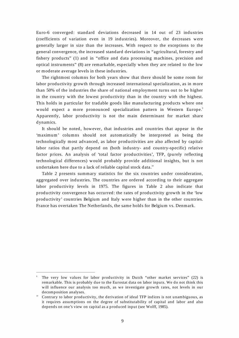
Euro-6 converged: standard deviations decreased in 14 out of 23 industries(coefficients of variation even in 19 industries). Moreover, the decreases weregenerally larger in size than the increases. With respect to the exceptions to thegeneral convergence, the increased standard deviations in “agricultural, forestry andfishery products” (1) and in “office and data processing machines, precision andoptical instruments” (8) are remarkable, especially when they are related to the lowor moderate average levels in these industries.
The rightmost columns for both years show that there should be some room forlabor productivity growth through increased international specialization, as in morethan 50% of the industries the share of national employment turns out to be higherin the country with the lowest productivity than in the country with the highest.This holds in particular for tradable goods like manufacturing products where onewould expect a more pronounced specialization pattern in Western Europe.9
Apparently, labor productivity is not the main determinant for market sharedynamics.
It should be noted, however, that industries and countries that appear in the‘maximum’ columns should not automatically be interpreted as being thetechnologically most advanced, as labor productivities are also affected by capital-labor ratios that partly depend on (both industry- and country-specific) relativefactor prices. An analysis of ‘total factor productivities’, TFP, (purely reflectingtechnological differences) would probably provide additional insights, but is notundertaken here due to a lack of reliable capital stock data.10
Table 2 presents summary statistics for the six countries under consideration,aggregated over industries. The countries are ordered according to their aggregatelabor productivity levels in 1975. The figures in Table 2 also indicate thatproductivity convergence has occurred: the rates of productivity growth in the ‘lowproductivity’ countries Belgium and Italy were higher than in the other countries.France has overtaken The Netherlands, the same holds for Belgium vs. Denmark.
9 The very low values for labor productivity in Dutch “other market services” (22) is
remarkable. This is probably due to the Eurostat data on labor inputs. We do not think thiswill influence our analysis too much, as we investigate growth rates, not levels in ourdecomposition analyses.
10 Contrary to labor productivity, the derivation of ideal TFP indices is not unambiguous, asit requires assumptions on the degree of substitutability of capital and labor and alsodepends on one’s view on capital as a produced input (see Wolff, 1985).
10
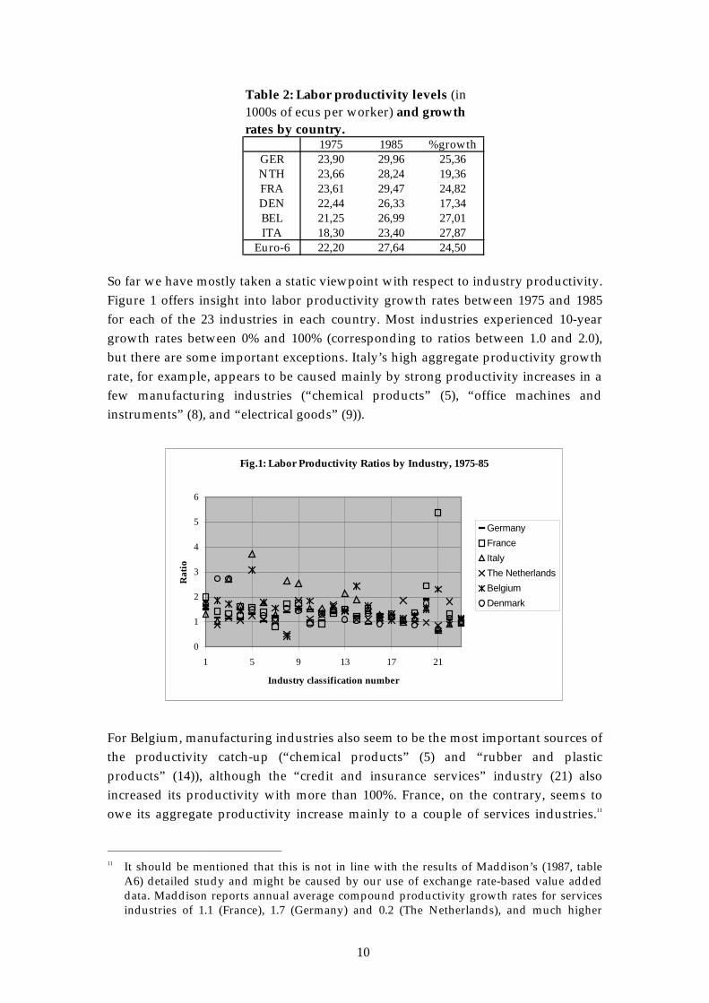
Table 2: Labor productivity levels (in 1000s of ecus per worker) and growthrates by country.
1975 1985 %growthGER 23,90 29,96 25,36NTH 23,66 28,24 19,36FRA 23,61 29,47 24,82DEN 22,44 26,33 17,34BEL 21,25 26,99 27,01ITA 18,30 23,40 27,87
Euro-6 22,20 27,64 24,50
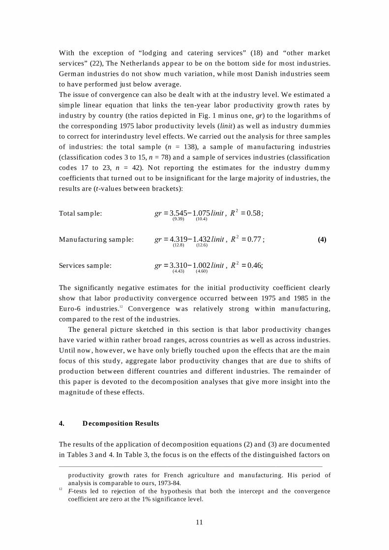
So far we have mostly taken a static viewpoint with respect to industry productivity.Figure 1 offers insight into labor productivity growth rates between 1975 and 1985for each of the 23 industries in each country. Most industries experienced 10-yeargrowth rates between 0% and 100% (corresponding to ratios between 1.0 and 2.0),but there are some important exceptions. Italy’s high aggregate productivity growthrate, for example, appears to be caused mainly by strong productivity increases in afew manufacturing industries (“chemical products” (5), “office machines andinstruments” (8), and “electrical goods” (9)).
Fig.1: Labor Productivity Ratios by Industry, 1975-85
0
1
2
3
4
5
6
1 5 9 13 17 21
Industry classification number
Rat
io
Germany
France
Italy
The Netherlands
Belgium
Denmark
For Belgium, manufacturing industries also seem to be the most important sources ofthe productivity catch-up (“chemical products” (5) and “rubber and plasticproducts” (14)), although the “credit and insurance services” industry (21) alsoincreased its productivity with more than 100%. France, on the contrary, seems toowe its aggregate productivity increase mainly to a couple of services industries.11
11 It should be mentioned that this is not in line with the results of Maddison’s (1987, table
A6) detailed study and might be caused by our use of exchange rate-based value addeddata. Maddison reports annual average compound productivity growth rates for servicesindustries of 1.1 (France), 1.7 (Germany) and 0.2 (The Netherlands), and much higher
11
With the exception of “lodging and catering services” (18) and “other marketservices” (22), The Netherlands appear to be on the bottom side for most industries.German industries do not show much variation, while most Danish industries seemto have performed just below average.The issue of convergence can also be dealt with at the industry level. We estimated asimple linear equation that links the ten-year labor productivity growth rates byindustry by country (the ratios depicted in Fig. 1 minus one, gr) to the logarithms ofthe corresponding 1975 labor productivity levels (linit) as well as industry dummiesto correct for interindustry level effects. We carried out the analysis for three samplesof industries: the total sample (n = 138), a sample of manufacturing industries(classification codes 3 to 15, n = 78) and a sample of services industries (classificationcodes 17 to 23, n = 42). Not reporting the estimates for the industry dummycoefficients that turned out to be insignificant for the large majority of industries, theresults are (t-values between brackets):
Total sample: OLQLWJU)4.10()39.9(
075.1545.3 −= , 58.02 =5 ;
Manufacturing sample: OLQLWJU)6.12()8.12(
432.1319.4 −= , 77.02 =5 ; (4)
Services sample: OLQLWJU)60.4()43.4(
002.1310.3 −= , ;46.02 =5
The significantly negative estimates for the initial productivity coefficient clearlyshow that labor productivity convergence occurred between 1975 and 1985 in theEuro-6 industries.12 Convergence was relatively strong within manufacturing,compared to the rest of the industries.
The general picture sketched in this section is that labor productivity changeshave varied within rather broad ranges, across countries as well as across industries.Until now, however, we have only briefly touched upon the effects that are the mainfocus of this study, aggregate labor productivity changes that are due to shifts ofproduction between different countries and different industries. The remainder ofthis paper is devoted to the decomposition analyses that give more insight into themagnitude of these effects.
4. Decomposition Results
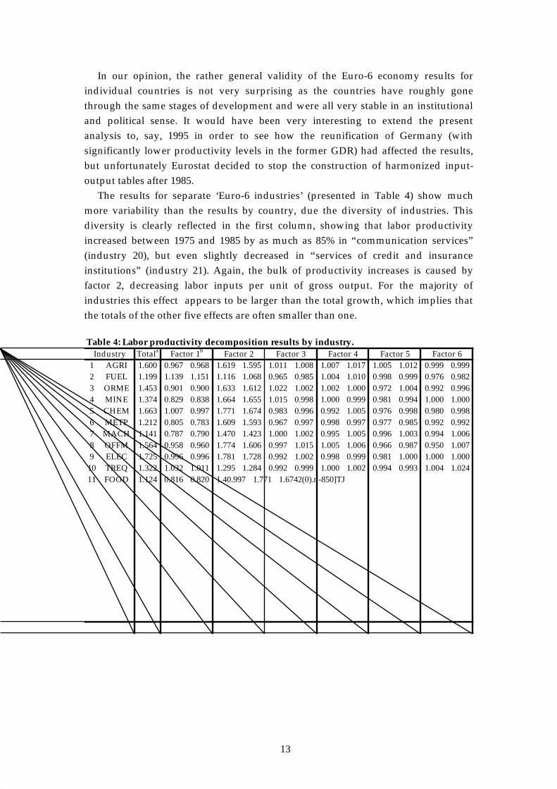
The results of the application of decomposition equations (2) and (3) are documentedin Tables 3 and 4. In Table 3, the focus is on the effects of the distinguished factors on
productivity growth rates for French agriculture and manufacturing. His period ofanalysis is comparable to ours, 1973-84.
12 F-tests led to rejection of the hypothesis that both the intercept and the convergencecoefficient are zero at the 1% significance level.
12
labor productivity levels for the six countries (aggregated over industries), Table 4emphasizes the effects on productivity levels for the 23 industries (aggregated overcountries).
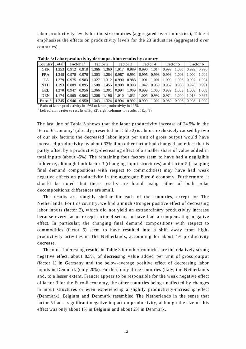
Table 3: Labor productivity decomposition results by countryCountry Totala Factor 1b Factor 2 Factor 3 Factor 4 Factor 5 Factor 6
GER 1.253 0.912 0.918 1.366 1.360 1.017 0.989 0.990 1.014 0.999 1.005 0.999 0.996FRA 1.248 0.978 0.976 1.303 1.284 0.987 0.991 0.995 0.998 0.998 1.003 1.000 1.004ITA 1.279 0.975 0.983 1.327 1.312 0.990 0.983 1.001 1.001 1.000 1.003 0.997 1.004
NTH 1.193 0.889 0.895 1.508 1.455 0.908 0.998 1.042 0.959 0.962 0.966 0.978 0.991BEL 1.270 0.947 0.956 1.366 1.301 0.994 1.009 0.999 1.000 0.982 1.003 1.008 1.008DEN 1.174 0.965 0.962 1.208 1.196 1.010 1.031 1.005 0.992 0.974 1.000 1.018 0.997
Euro-6 1.245 0.946 0.950 1.343 1.324 0.994 0.992 0.999 1.002 0.989 0.996 0.998 1.000a Ratio of labor productivity in 1985 to labor productivity in 1975.b Left columns refer to results of Eq. (2), right columns to results of Eq. (3)
The last line of Table 3 shows that the labor productivity increase of 24.5% in the‘Euro- 6 economy’ (already presented in Table 2) is almost exclusively caused by twoof our six factors: the decreased labor input per unit of gross output would haveincreased productivity by about 33% if no other factor had changed, an effect that ispartly offset by a productivity-decreasing effect of a smaller share of value added intotal inputs (about -5%). The remaining four factors seem to have had a negligibleinfluence, although both factor 3 (changing input structures) and factor 5 (changingfinal demand compositions with respect to commodities) may have had weaknegative effects on productivity in the aggregate Euro-6 economy. Furthermore, itshould be noted that these results are found using either of both polardecompositions: differences are small.
The results are roughly similar for each of the countries, except for TheNetherlands. For this country, we find a much stronger positive effect of decreasinglabor inputs (factor 2), which did not yield an extraordinary productivity increasebecause every factor except factor 4 seems to have had a compensating negativeeffect. In particular, the changing final demand compositions with respect tocommodities (factor 5) seem to have resulted into a shift away from high-productivity activities in The Netherlands, accounting for about 4% productivitydecrease.
The most interesting results in Table 3 for other countries are the relatively strongnegative effect, about 8.5%, of decreasing value added per unit of gross output(factor 1) in Germany and the below-average positive effect of decreasing laborinputs in Denmark (only 20%). Further, only three countries (Italy, the Netherlandsand, to a lesser extent, France) appear to be responsible for the weak negative effectof factor 3 for the Euro-6 economy, the other countries being unaffected by changesin input structures or even experiencing a slightly productivity-increasing effect(Denmark). Belgium and Denmark resembled The Netherlands in the sense thatfactor 5 had a significant negative impact on productivity, although the size of thiseffect was only about 1% in Belgium and about 2% in Denmark.

15
Second, it is a well-known fact that quality differences are seldom fully reflectedin prices. Deflation procedures may yield relatively low productivity measures forindustries that produce ‘high-quality varieties’ of a good.13 Keeping this in mind, itwould not be that strange if an industry with a low productivity level or a lowproductivity growth rate (compared to its foreign competitors) would not losemarket share.
A third potential cause, related to the interindustry nature of final demand goodproduction is investigated in the next section.
5. Productivity Analysis of Vertically Integrated Industries
Labor productivity changes in an individual industry can be due to a number of ‘realproductivity factors’, of which capital deepening and technological progress are thebest recognized ones, but can also be caused by a changing underlying activitystructure. A well-known example is the contracting out of accounting and/orcleaning activities by manufacturing firms to specialized firms: on the aggregate thesame work may be done by an identical amount of employees, but the productivityfigures of the manufacturing firm are likely to change. We can get rid of these effectsby taking a different perspective, in which the ratio between value added and laborneeded in the production of one unit of final demand output is the main variable.
The alternative approach does not consider industries in the usual sense, butinvestigates “vertically integrated industries” (Pasinetti, 1973) that consist of allindustries that directly or indirectly contribute to the production of a final demandcommodity, weighted by their respective contributions.14 Such an approach mightindicate a potential solution to the previous section’s somewhat paradoxical resultthat final demand for tradable goods did not shift towards countries in which levelsand growth rates of labor productivity in the industries concerned were relativelyhigh. A hypothetical example might clarify the claim for a potential solution.
Suppose a situation in which labor productivity in the “food, beverages andtobacco” industry (in country A) is decreasing and productivity in its main supplierindustry “agricultural, forestry and fishery products” (in the same country) isincreasing, while labor productivity levels for these industries are constant in theother countries. Then, an increasing share of country A in final demand for “food,etc.” might seem strange at first sight if one assumes that low labor productivity
13 In fact, conventional price deflators “shift” productivity increases from the quality-
increasing industry to the industries buying its product. For example, it may well be thatpart of the 85% labor productivity increase in “communication services” is due toproductivity increases that should actually be accounted for in “office and data processingmachinery” in the same or a second country (see, e.g. Los, 1997, for a discussion of theseso-called “rent spillovers”). In this paper, however, we focus on ‘conventionally measured’prices and productivity levels.
14 So accounting and cleaning activities always turn up in the productivity of the verticallyintegrated industry that produces a certain manufactured good, no matter whether theseactivities are contracted out or not.
16
levels are reflected in high prices (wage rate differences, for instance, might disturbsuch relationships). In fact, however, labor is not the only input the use of whichmay be reflected in output prices: next to fixed capital goods, intermediate inputs areoften required. Bearing this in mind, the relatively low price paid for “agriculturalproducts, etc.” might allow country A to set the price for its “food, etc.” equal to orbelow that of foreign competitors, depending on the shares of “agriculturalproducts, etc.” in total inputs. Extending this reasoning, labor productivity changesin any of the upstream industries might well affect the final demand market sharesof a country for a given output. The concept of vertically integrated industriesaccounts for this notion. Hence, labor productivity changes in vertically integratedindustries are the central issue in this section.
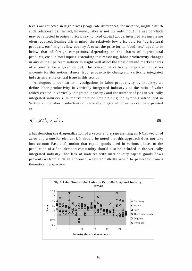
Analogous to our earlier investigations in labor productivity by industry, wedefine labor productivity in vertically integrated industry i as the ratio of valueadded created in vertically integrated industry i and the number of jobs in verticallyintegrated industry i. In matrix notation (maintaining the symbols introduced inSection 2), the labor productivity of vertically integrated industry i can be expressedas
LL
3
LHI/HI/ ˆ'ˆ' λµπ = , (5)
a hat denoting the diagonalization of a vector and ei representing an NCx1 vector ofzeros and a one for element i. It should be noted that this approach does not takeinto account Pasinetti’s notion that capital goods used in various phases of theproduction of a final demand commodity should also be included in the verticallyintegrated industry. The lack of matrices with interindustry capital goods flowsprevents us from such an approach, which admittedly would be preferable from atheoretical perspective.
Fig. 2: Labor Productivity Ratios by Vertically Integrated Industry, 1975-85
0,5
0,75
1
1,25
1,5
1,75
2
2,25
1 5 9 13 17 21
Industry classification number
Rat
io
Germany
France
Italy
The Netherlands
Belgium
Denmark
17
Figure 2 presents an overview of labor productivity developments in all 23 verticallyintegrated industries (each representing one final demand output) for each of the sixcountries.15 In general, the results are similar to those plotted in Fig. 1. Themagnitudes of the ratios, however, are far less dispersed, which does not come as asurprise as all ratios can be interpreted as weighted averages of those plotted in Fig.1. The Netherlands did not perform well compared to other countries, except for thevertically integrated industries 18 (“final demand of lodging and catering services”)and 22 (“final demand of other market services”). France did well in several finaldemand services, but in a vertically integrated industry context the main Frenchwinner is not “final demand of credit and insurance services” (21), but “finaldemand of communication services” (20). Italy is again strong in final demand ofvarious manufactured commodities. Further, Belgian vertically integrated industries5 (“final demand of chemical products”) and 14 (“final demand of rubber and plasticproducts”) managed to attain high scores, the latter not only because the Belgianrubber and plastic industry itself shows a high productivity growth, but also becausea large share of total inputs was supplied by the Belgian chemical industry with anextremely strong productivity growth (see Fig. 1).
Like for industries in the more usual sense, we carried out some regressions to seewhether convergence at the level of vertically integrated industries occurredbetween 1975 and 1985. Labor productivity increases (grp) were again linked to thelogarithms of productivity levels in 1975 (linitp) and a series of industry dummies.The regressions were run for the total sample, the sample of vertically integratedindustries producing manufacturing goods and the sample of vertically integratedindustries producing services.
Total sample: OLQLWSJUS)23.4()55.4(
228.0828.0 −= , 41.02 =5 ;
Manufacturing sample: OLQLWSJUS)00.3()51.3(
206.0783.0 −= , 43.02 =5 ; (6)
Services sample: OLQLWSJUS)32.2()64.2(
303.0049.1 −= , ;34.02 =5
Again the null hypothesis of zero convergence is rejected at usual levels ofsignificance.16 Nevertheless, the differences with the regression results obtained forindustries in the usual sense are clear. First, the estimated convergence rates are
15 Note that our intercountry framework implies that labor productivity growth for vertically
integrated industries in a given country may also be affected by labor productivity changesin one or more of the other countries included in the analysis.
16 With respect to the total sample as well as the manufacturing sample, not only t-valueslead to rejection. F-tests on the simultaneous significance of the constant and theconvergence coefficient yield values that correspond to p-values well below 0.01 and 0.025,respectively. For services, the null of a zero constant and a zero convergence coefficientcould only be rejected at a 10% significance level, so convergence may be absent withinthis subsample.

18
much lower (0.2 to 0.3 versus 1.0 to 1.4), which is likely to be a consequence of a lesspronounced variability of initial productivity levels across vertically integratedindustries. Second, the coefficients of determination are lower for the case ofvertically integrated industries. This difference is especially marked for themanufacturing sample: 0.43 versus 0.77.
The labor productivity ratios by vertically integrated industry plotted in Figure 2can be decomposed into the first four factors of equations (2) and (3). The last twofactors do not play a role, as final demand changes have no impact on laborproductivity levels of individual vertically integrated industries, so we replaced thefinal demand vectors in equations (2) and (3) by vectors consisting of zeros exceptfor a one for the element corresponding to the vertically integrated industry underinvestigation (ei).
17 For reasons of space, we restrict our documentation of results totwo diagrams that offer insight into the effects that are central to our analysis: theeffects of input structure changes and those of trade structure changes.
F i g . 3 : I n p u t S t r u c t u r e E f f e c t R a t i o s b y V e r t i c a l l y I n t e g r a t e dI n d u s t r y , 1 9 7 5 - 8 5
I n d u s t r y c l a s s i f i c a t i o n n u m b e r
T h e N e t h e r l a n d sF i g u r e 3 s h o w s t h a t t h e m a j o r i t y o f i n p u t s t r u c t u r e e f f e c t r a t i o s a r e c l o s e t o 1 . 0 , w h i c h i s h a r d l y s u r p r i s i n g a f t e r o u r p r e v i o u s a n a l y s i s . N e v e r t h e l e s s , s o m e i n t e r e s t i n g f e a t u r e s e m e r g e f r o m t h e d i a g r a m . T h e c o m p a r a t i v e l y w e a k l a b o r p r o d u c t i v i t y
g r o w t h f o r T h e N e t h e r l a n d s s e e m s t o b e p a r t l y c a u s e d b y n e g a t i v e i n p u t s t r u c t u r e
e f f e c t s : f o r a l m o s t a l l v e r t i c a l l y i n t e g r a t e d i n d u s t r i e s t h e D u t c h r a t i o s a r e t h e l o w e s t .
T h e o p p o s i t e i s t r u e f o r D e n m a r k ( a l t h o u g h s o m e w h a t l e s s m a r k e d ) , w i t h a n
e x t r e m e l y l a r g e p o s i t i v e e f f e c t f o r t h e ‘ f i n a l d e m a n d c r e d i t a n d i n s u r a n c e s e r v i c e s
i n d u s t r y ’ . I t a p p e a r s f r o m F i g u r e 4 t h a t t r a d e s t r u c t u r e e f f e c t s h a v e n o t b e e n
p a r t i c u l a r l y f a v o r a b l e t o t h e D u t c h v e r t i c a l l y i n t e g r a t e d i n d u s t r i e s , t o o . P a r t o f I t a l y ’ s
g o o d p e r f o r m a n c e i n m a n u f a c t u r i n g s e e m s t o h a v e b e e n d u e t o t r a d e s t r u c t u r e
c h a n g e s , a l t h o u g h t h e e f f e c t s s e l d o m e x c e e d 1 % : “ f i n a l d e m a n d o f f i c e m a c h i n e r y a n d
I n f a c t , e q u a t i o n ( 4 ) c o u l d b e s i m p l i f i e d k e e p i n g i n m i n d t h a t v a l u e a d d e d a n d l a b o r p e r
u n i t o f f i n a l d e m a n d a n d , . r e s p e c t i v e l y .
F i g u r e s 3 a n d 4 p r e s e n t a v e r a g e s o v e r t h e t w o d e c o m p o s i t i o n s a n a l o g o u s t o e q u a t i o n s ( 2 )
a n d ( 3 ) .
19
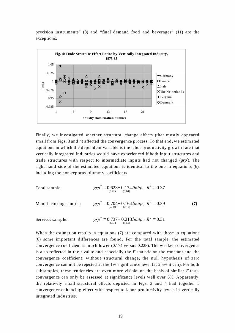
precision instruments” (8) and “final demand food and beverages” (11) are theexceptions.
Finally, we investigated whether structural change effects (that mostly appearedsmall from Figs. 3 and 4) affected the convergence process. To that end, we estimatedequations in which the dependent variable is the labor productivity growth rate thatvertically integrated industries would have experienced if both input structures andtrade structures with respect to intermediate inputs had not changed (grp*). Theright-hand side of the estimated equations is identical to the one in equations (6),including the non-reported dummy coefficients.
Total sample: OLQLWSJUS)04.3()22.3(
* 174.0623.0 −= , 37.02 =5
Manufacturing sample: OLQLWSJUS)19.2()90.2(
* 164.0704.0 −= , 39.02 =5 (7)
Services sample: OLQLWSJUS)55.1()77.1(
* 213.0737.0 −= , 31.02 =5
When the estimation results in equations (7) are compared with those in equations(6) some important differences are found. For the total sample, the estimatedconvergence coefficient is much lower (0.174 versus 0.228). The weaker convergenceis also reflected in the t-value and especially the F-statistic on the constant and theconvergence coefficient: without structural change, the null hypothesis of zeroconvergence can not be rejected at the 1% significance level (at 2.5% it can). For bothsubsamples, these tendencies are even more visible: on the basis of similar F-tests,convergence can only be assessed at significance levels well over 5%. Apparently,the relatively small structural effects depicted in Figs. 3 and 4 had together aconvergence-enhancing effect with respect to labor productivity levels in verticallyintegrated industries.
Fig. 4: Trade Structure Effect Ratios by Vertically Integrated Industry, 1975-85
0,925
0,95
0,975
1
1,025
1,05
1 5 9 13 17 21
Industry classification number
Rat
io
Germany
France
Italy
The Netherlands
Belgium
Denmark
20
All in all, the analysis of labor productivity from a vertically integrated industryviewpoint does not alter our previous conclusion that neither input structurechanges nor trade structure changes significantly contributed to the growth of laborproductivity in the Euro-6 economy. Convergence of productivity levels, however,was enhanced by these structural effects.
6. Summary and Conclusions
The application of a new aggregate labor productivity growth decompositionframework on two full intercountry input-output tables in constant prices for sixWestern European countries has shown that productivity effects of input structurechanges and of trade structure effects are rather small compared to those of growinglabor productivity levels in individual industries. Although convergence in verticallyintegrated industries was enhanced by structural change, most of the relatively fewsignificant structure effects on growth are even negative, which implies that laborproductivity growth would have been higher if no structure changes had occurred(at least if one is willing to maintain the assumption common to growth accountingand structural change decomposition studies that the constituent parts of aggregategrowth are independent). This is somewhat surprising, as our summary statistics onproductivity levels indicate that aggregate Euro-6 productivity allows for asignificant growth, by a mere increase in international specialization.
A number of potential explanations for this result can be formulated. Theprobably most important of them was argued to be the imperfect reflection ofproductivity differentials in prices. We mention four additional candidates thatmight explain the results above, the first two being related to our methodology andthe latter two dealing with the time period and economies we investigated. First, ourinput-output tables were constructed using exchange rate-conversions of values innational currencies, instead of more appropriate PPP-conversions. Second, we werenot able to decompose growth rate differences between two periods of time, as wehad only two input-output tables available. Wolff (1985) provides some evidencethat structural change effects (at least within a country) are more important in thatkind of decompositions. Third, our period under investigation (10 years) may not belong enough to find significant positive effects, for example because structures donot adapt very quickly to changing technological or economic changes. Finally, oursample of countries may not be heterogeneous enough (despite the reportedproductivity differences) to cause important shifts of (labor) resources acrossindustries, bearing in mind that transaction costs as well as transportation costs mustbe compensated for by price differentials before a firm might be tempted to buy itsinputs abroad.
Following the argument of a lack of heterogeneity in our sample, we think that itwould be a promising avenue of research to apply our decomposition formulae to a
21
set of intercountry input-output tables for e.g. the U.S. (or even their individualstates) and Mexico, to see how input structure and trade structure changes followingNAFTA affected labor productivity in both countries or their states. Anotherinteresting case might emerge if former Eastern Block countries enter the EuropeanUnion. The construction of the required tables would not be without difficulties,however, in particular if one would try to use more appropriate currency converters.Nevertheless, we think that studies like the present one contribute to the merits ofsuch tables.
References
Barro, R.J. and X. Sala-i-Martin (1992), “Convergence”, Journal of Political Economy, vol. 100,
pp. 223-251.
Baumol, W.J. (1986), “Productivity Growth, Convergence, and Welfare: What the Long Run
Data Show”, American Economic Review, vol. 76, pp. 1072-1085.
Bernard, A.W. and C.I. Jones (1996), “Productivity across Industries and Countries: Time
Series Theory and Evidence”, Review of Economics and Statistics, vol. 78, pp. 135-146.
Carter, A.P. (1970), Structural Change in the American Economy, Harvard University Press,
Cambridge MA.
Casler, S.D. and M.S. Gallatin (1997), “Sectoral Contributions to Total Factor Productivity:
Another Perspective on the Growth Slowdown”, Journal of Macroeconomics, vol. 19, pp. 381-
393.
Chenery, H.B., S. Shishido and T. Watanabe (1962), “The Pattern of Japanese Growth, 1914-
1954”, Econometrica, vol. 30, pp. 98-139.
De Long, D.B. (1988), “Productivity Growth, Convergence and Welfare: Comment”, American
Economic Review, vol. 78, pp. 1138-1154.
Denison, E.F. (1967), Why Growth Rates Differ, Brookings Institution, Washington DC.
Dietzenbacher, E. (1997), “An Intercountry Decomposition of Output Growth in EC
Countries”, paper presented at the 44th North-American Meeting of the Regional Science
Association, November 6-9, Buffalo NY.
Dietzenbacher, E., J.A. Van der Linden and A.E. Steenge (1993), “The Regional Extraction
Method: Applications to the European Community”, Economic Systems Research, vol. 5, pp.
185-206.
Dietzenbacher, E. and J.A. Van der Linden (1997), “Sectoral and Spatial Linkages in the EC
Production Structure”, Journal of Regional Science, vol. 37, pp. 235-257.
Dietzenbacher, E. and B. Los (1997), “Analyzing Decomposition Analyses”, in: A. Simonovits
and A.E. Steenge (eds.), Prices, Growth and Cycles, Macmillan, London, pp. 108-131.
Dietzenbacher, E. and B. Los (1998), “Structural Decomposition Techniques: Sense and
Sensitivity”, Economic Systems Research, vol. 10, forthcoming.
22
Dixon, R.J. and A.P. Thirlwall (1975), “A Model of Regional Growth Rate Differences on
Kaldorian Lines”, Oxford Economic Papers, vol. 11, pp. 201-214.
Dollar, D. and E.N. Wolff (1993), Competitiveness, Convergence, and International Specialization,
MIT Press, Cambridge MA.
Dowrick, S. and D.T. Nguyen (1989), “OECD Comparative Economic Growth 1950-85: Catch-
Up and Convergence”, American Economic Review, vol. 79, pp. 1010-1030.
Eurostat (1979), European System of Integrated Economic Accounts, ESA, 2nd edition,
Luxembourg.
Eurostat (1986), National Accounts ESA: Detailed Tables by Branch, 1986, Luxembourg.
Eurostat (1988), National Accounts ESA: Detailed Tables by Branch, 1988, Luxembourg.
Eurostat (1989), National Accounts ESA: Detailed Tables by Branch, 1989, Luxembourg.
Eurostat (1990), External Trade Statistics: User’s Guide, Luxembourg.
Eurostat (1991), National Accounts ESA: Detailed Tables by Branch, 1980-1988, Luxembourg.
Fagerberg, J. (1988), “International Competitiveness”, Economic Journal, vol. 98, pp. 355-374.
Feldman, S.J., D. McClain and K. Palmer (1987), “Sources of Structural Change in the United
States”, Review of Economics and Statistics, vol. 69, pp. 503-510.
Galatin, M. (1988), “Technical Change and the Measurement of Productivity in an Input-
Output Model”, Journal of Macroeconomics, vol. 10, pp. 613-632.
Grossman, G.M. and E. Helpman (1990), “Comparative Advantage and Long Run Growth”,
American Economic Review, vol. 80, pp. 796-815.
Hoen, A.R. (1998), Ph.D. Thesis, University of Groningen, forthcoming.
Jorgenson, D.W., F.M. Gollop and B.M. Fraumeni (1987), Productivity and U.S. Economic
Growth, Harvard University Press, Cambridge MA.
Los, B. (1997), “A Review of Interindustry Technology Spillover Measurement Methods”,
Working Paper, University of Twente.
Los, B. and B. Verspagen (1997), “R&D Spillovers and Productivity: Evidence from U.S.
Manufacturing Microdata”, MERIT Research Memorandum 96/007, University of
Maastricht.
Lucas, R.E. (1988), “On the Mechanisms of Economic Development”, Journal of Monetary
Economics, vol. 22, pp. 3-42.
Maddison, A. (1987), “Growth and Slowdown in Advanced Capitalist Economies: Techniques
of Quantitative Assessment”, Journal of Economic Literature, vol. 25, pp. 649-698.
Maddison, A. and B. van Ark (1989), “International Comparison of Purchasing Power, Real
Output and Labour Productivity: A Case Study of Brazilian, Mexican and US
Manufacturing, 1975”, Review of Income and Wealth, vol. 35, pp. 31-55.
Oosterhaven, J., A.R. Hoen and J.A. Van der Linden (1995), “Technology, Trade and Real
Value Added Growth of EC Countries, 1975-1985”, paper presented at the XIth
International Conference in Input-Output Techniques, 27 november-1 december, New
Delhi, India.
Oosterhaven, J. and J.A. van der Linden (1997), “European Technology, Trade and Income
Changes for 1975-85: An Intercountry Input-Output Decomposition”, Economic Systems
Research, vol. 9, pp. 393-412.
23
Pasinetti, L.L. (1973), “The Notion of Vertical Integration in Economic Analysis”,
Metroeconomica, vol. 25, pp. 1-29.
Romer, P.M. (1990), “Endogenous Technological Change”, Journal of Political Economy, vol. 98,
pp. S71-S102.
Rose, A. and S. Casler (1996), “Input-Output Structural Decomposition Analysis: A Critical
Appraisal”, Economic Systems Research, vol. 8, pp. 33-62.
Skolka, J. (1989), “Input-Output Structural Decomposition Analysis for Austria”, Journal of
Policy Modeling, vol. 11, pp. 45-66.
Solow, R.M. (1956), “A Contribution to the Theory of Economic Growth”, Quarterly Journal of
Economics, vol. 70, pp. 65-94.
Statistics Netherlands (1996), Time Series Labor Accounts 1969-1993, Heerlen/Voorburg.
Swan, T.W. (1956), “Economic Growth and Capital Accumulation”, Economic Record, vol. 32,
pp. 334-361.
Van der Linden, J.A. and J. Oosterhaven (1995), “EC Intercountry Input-Output Relations:
Construction Method and Main Results for 1965-1985, Economic Systems Research, vol. 7, pp.
249-270.
Verspagen, B. (1991), “A New Empirical Approach to Catching Up or Falling Behind”,
Structural Change and Economic Dynamics, vol. 2, pp. 359-380.
Verspagen, B. (1997), “Estimating International Technology Spillovers Using Technology Flow
Matrices”, Weltwirtschaftliches Archiv, vol. 133, pp. 226-248.
Wolff, E.N. (1985), “Industrial Composition, Interindustry Effects, and the U.S. Productivity
Slowdown”, Review of Economics and Statistics, vol. 67, pp. 268-277.
Wolff, E.N. (1994), “Productivity Measurement within an Input-Output Framework”, Regional
Science and Urban Economics, vol. 24, pp. 75-92.
24
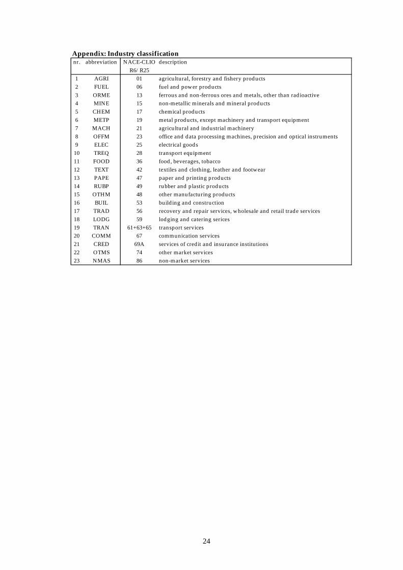
Appendix: Industry classificationnr. abbreviation NACE-CLIO description
R6/R251 AGRI 01 agricultural, forestry and fishery products2 FUEL 06 fuel and power products3 ORME 13 ferrous and non-ferrous ores and metals, other than radioactive4 MINE 15 non-metallic minerals and mineral products5 CHEM 17 chemical products6 METP 19 metal products, except machinery and transport equipment7 MACH 21 agricultural and industrial machinery8 OFFM 23 office and data processing machines, precision and optical instruments9 ELEC 25 electrical goods
10 TREQ 28 transport equipment11 FOOD 36 food, beverages, tobacco12 TEXT 42 textiles and clothing, leather and footwear13 PAPE 47 paper and printing products14 RUBP 49 rubber and plastic products15 OTHM 48 other manufacturing products16 BUIL 53 building and construction17 TRAD 56 recovery and repair services, wholesale and retail trade services18 LODG 59 lodging and catering serices19 TRAN 61+63+65 transport services20 COMM 67 communication services21 CRED 69A services of credit and insurance institutions22 OTMS 74 other market services23 NMAS 86 non-market services
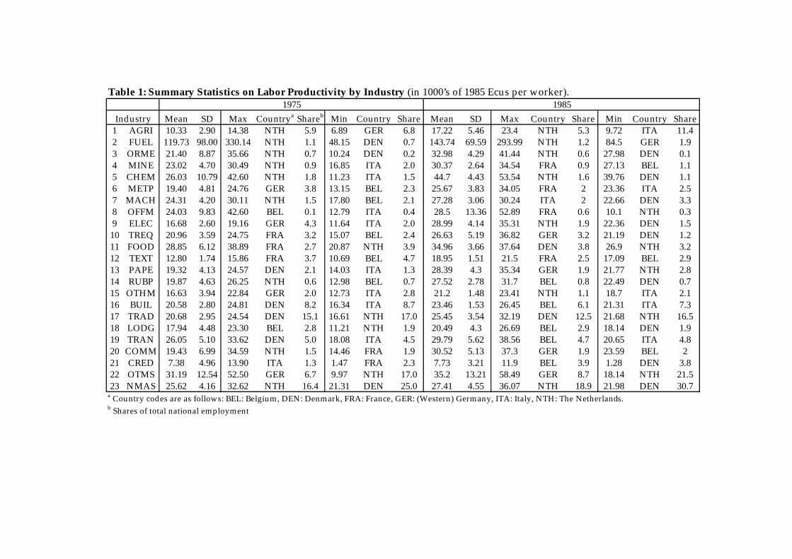
Table 1: Summary Statistics on Labor Productivity by Industry (in 1000’s of 1985 Ecus per worker).1975 1985
Industry Mean SD Max Countrya Shareb Min Country Share Mean SD Max Country Share Min Country Share1 AGRI 10.33 2.90 14.38 NTH 5.9 6.89 GER 6.8 17.22 5.46 23.4 NTH 5.3 9.72 ITA 11.42 FUEL 119.73 98.00 330.14 NTH 1.1 48.15 DEN 0.7 143.74 69.59 293.99 NTH 1.2 84.5 GER 1.93 ORME 21.40 8.87 35.66 NTH 0.7 10.24 DEN 0.2 32.98 4.29 41.44 NTH 0.6 27.98 DEN 0.14 MINE 23.02 4.70 30.49 NTH 0.9 16.85 ITA 2.0 30.37 2.64 34.54 FRA 0.9 27.13 BEL 1.15 CHEM 26.03 10.79 42.60 NTH 1.8 11.23 ITA 1.5 44.7 4.43 53.54 NTH 1.6 39.76 DEN 1.16 METP 19.40 4.81 24.76 GER 3.8 13.15 BEL 2.3 25.67 3.83 34.05 FRA 2 23.36 ITA 2.57 MACH 24.31 4.20 30.11 NTH 1.5 17.80 BEL 2.1 27.28 3.06 30.24 ITA 2 22.66 DEN 3.38 OFFM 24.03 9.83 42.60 BEL 0.1 12.79 ITA 0.4 28.5 13.36 52.89 FRA 0.6 10.1 NTH 0.39 ELEC 16.68 2.60 19.16 GER 4.3 11.64 ITA 2.0 28.99 4.14 35.31 NTH 1.9 22.36 DEN 1.510 TREQ 20.96 3.59 24.75 FRA 3.2 15.07 BEL 2.4 26.63 5.19 36.82 GER 3.2 21.19 DEN 1.211 FOOD 28.85 6.12 38.89 FRA 2.7 20.87 NTH 3.9 34.96 3.66 37.64 DEN 3.8 26.9 NTH 3.212 TEXT 12.80 1.74 15.86 FRA 3.7 10.69 BEL 4.7 18.95 1.51 21.5 FRA 2.5 17.09 BEL 2.913 PAPE 19.32 4.13 24.57 DEN 2.1 14.03 ITA 1.3 28.39 4.3 35.34 GER 1.9 21.77 NTH 2.814 RUBP 19.87 4.63 26.25 NTH 0.6 12.98 BEL 0.7 27.52 2.78 31.7 BEL 0.8 22.49 DEN 0.715 OTHM 16.63 3.94 22.84 GER 2.0 12.73 ITA 2.8 21.2 1.48 23.41 NTH 1.1 18.7 ITA 2.116 BUIL 20.58 2.80 24.81 DEN 8.2 16.34 ITA 8.7 23.46 1.53 26.45 BEL 6.1 21.31 ITA 7.317 TRAD 20.68 2.95 24.54 DEN 15.1 16.61 NTH 17.0 25.45 3.54 32.19 DEN 12.5 21.68 NTH 16.518 LODG 17.94 4.48 23.30 BEL 2.8 11.21 NTH 1.9 20.49 4.3 26.69 BEL 2.9 18.14 DEN 1.919 TRAN 26.05 5.10 33.62 DEN 5.0 18.08 ITA 4.5 29.79 5.62 38.56 BEL 4.7 20.65 ITA 4.820 COMM 19.43 6.99 34.59 NTH 1.5 14.46 FRA 1.9 30.52 5.13 37.3 GER 1.9 23.59 BEL 221 CRED 7.38 4.96 13.90 ITA 1.3 1.47 FRA 2.3 7.73 3.21 11.9 BEL 3.9 1.28 DEN 3.822 OTMS 31.19 12.54 52.50 GER 6.7 9.97 NTH 17.0 35.2 13.21 58.49 GER 8.7 18.14 NTH 21.523 NMAS 25.62 4.16 32.62 NTH 16.4 21.31 DEN 25.0 27.41 4.55 36.07 NTH 18.9 21.98 DEN 30.7
a Country codes are as follows: BEL: Belgium, DEN: Denmark, FRA: France, GER: (Western) Germany, ITA: Italy, NTH: The Netherlands. b Shares of total national employment