Embed Size (px)
DESCRIPTION
control fuente
Citation preview
1
EML 5311 - Spring 2009University of Florida
Mechanical & Aerospace EngineeringFinal ProjectDue 4/22/09
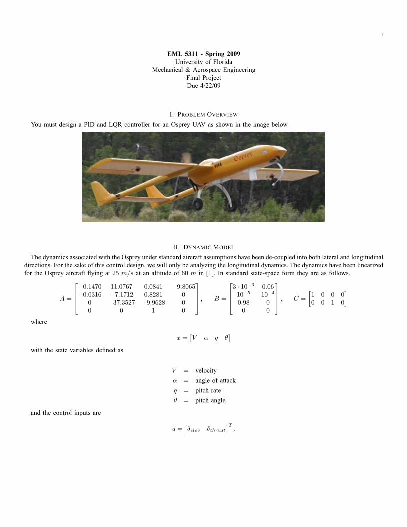
I. PROBLEM OVERVIEWYou must design a PID and LQR controller for an Osprey UAV as shown in the image below.
II. DYNAMIC MODELThe dynamics associated with the Osprey under standard aircraft assumptions have been de-coupled into both lateral and longitudinal
directions. For the sake of this control design, we will only be analyzing the longitudinal dynamics. The dynamics have been linearizedfor the Osprey aircraft �ying at 25 m=s at an altitude of 60 m in [1]. In standard state-space form they are as follows.
A =
2664�0:1470 11:0767 0:0841 �9:8065�0:0316 �7:1712 0:8281 0
0 �37:3527 �9:9628 00 0 1 0
3775 , B =
26643 � 10�3 0:0610�5 10�4
0:98 00 0
3775 , C =
�1 0 0 00 0 1 0
�
where
x =�V � q �
�with the state variables de�ned as
V = velocity� = angle of attackq = pitch rate� = pitch angle
and the control inputs are
u =��elev �thrust
�T:
2
III. CONTROL OBJECTIVESDesign a single controller that yields the following desired criteria over the widest possible initial conditions.1) Stabilize the system with a velocity step input of 10 m=s.2) Minimize rise time, % overshoot, and steady state error.3) Actuator limits and sensor noise:
� The maximum �thrust is �200 N and �200 N=sec� The maximum �elev is .�30�and �300�=s� The noise for the velocity sensor is �0:4 m=s� The noise for the pitch rate sensor is �1:7�=s
IV. EXPECTATIONS1) Perform 3 control designs
� a PID controller� a LQR controller (full state feedback, hence C = I4x4)� a LQR controller plus observer (with C de�ned as in the dynamic model section)
2) Prepare a Report: As the control design engineer, you must prove to the management that your controller will work as desired,or why the stated criteria can not be met. To this end, a signi�cant portion of the grade relies on your ability to effectivelycommunicate your results to the management. As a manager I need ALL the details to make an informed decision, but I alsoneed to look at the answers quickly and get the "snapshot answer" in minutes. Your report should discuss and compare theresults from the controllers. Discuss the performance for different initial conditions, with the noise effects, and (as a third case)model error (i.e., parameters in A and B are not precise). Evaluate gain and phase margins and discuss the sensitivity andcomplimentary sensitivity.
REFERENCES[1] W. MacKunis, M. K. Kaiser, P. M. Patre, and W. E. Dixon, �Asymptotic tracking for aircraft via an uncertain dynamic inversion method,� in American
Control Conf., Seattle, WA, June 2008, pp. 3482�3487.

Page 1 of 33
Ramin Shamshiri EML 5311, Final Project Due 30/04/09
EML 5311, Section 2484 Final Project
Due Wednesday, April 30th, 2009
RAMIN SHAMSHIRI UFID#: 9021-3353

Page 2 of 33
Ramin Shamshiri EML 5311, Final Project Due 30/04/09
I. Problem overview: Design a PID and LQR controller for an Osprey UAQ as shown in the image below.
II. Dynamic Model: The dynamics associated with the Osprey under standard aircraft assumptions have been de-coupled into both lateral and longitudinal directions. For the sake of this control design, we will only be analyzing the longitudinal dynamics. The dynamics have been linearized for the Osprey aircraft flying at 25 m/s at an altitude of 60 m in [1]. In standard state-space form they are as follows.
𝐴 =
−0.1470 11.0767 0.0841 −9.8065−0.0316 −7.1712 0.8281 0
0 −37.3527 −9.9628 00 0 1 0
𝐵 =
3.10−3 0.0610−5 10−4
0.98 00 0
𝐶 = 1 0 0 00 0 1 0
where 𝑥 = 𝑉 𝛼 𝑞 𝜃 With the state variables defined as: 𝑉 = Velocity 𝛼 = Angle of attack 𝑞 = Pitch rate 𝜃 =Pitch angle and the control inputs are:
𝑢 = 𝛿𝑒𝑙𝑒𝑣
𝛿𝑡ℎ𝑟𝑢𝑠𝑡

Page 3 of 33
Ramin Shamshiri EML 5311, Final Project Due 30/04/09
III. Control objective: Design a single controller that yields the following desired criteria over the widest possible initial conditions.
1. Stabilize the system with a velocity step input of 10m/s. 2. Minimize rise time, % overshoot, and steady state error. 3. Actuator limits and sensor noise:
The maximum 𝛿𝑡ℎ𝑟𝑢𝑠𝑡 is ±200 𝑁 and ±200 𝑁/𝑠𝑒𝑐 The maximum 𝛿𝑒𝑙𝑒𝑣 is ±30°and ±300°/𝑠 The noise for the velocity sensor is ±0.4 𝑚/𝑠 The noise for the pitch rate sensor is ±1.7°/𝑠
IV. Expectations:
1- Perform 3 control designs
A PID controller A LQR controller (full state feedback, hence 𝐶 = 𝐼4×4 ) A LQR controller plus observer (with 𝐶 defined as in the dynamic model section)
2- Prepare a report:
As the control design engineer, you must you must prove to the management that your controller will work as desired, or why the stated criteria cannot be met. To this end, a significant portion of the grade relies on your ability to effectively communicate your results to the management. As a manager I need ALL the details to make an informed decision, but I also need to look at the answers quickly and get the "snapshot answer" in minutes. Your report should discuss and compare the results from the controllers. Discuss the performance for different initial conditions, with the noise effects, and (as a third case) model error (i.e., parameters in A and B are not precise). Evaluate gain and phase margins and discuss the sensitivity and complimentary sensitivity.

Page 4 of 33
Ramin Shamshiri EML 5311, Final Project Due 30/04/09
Solution:
Creating model in MATLAB: % Dynamic Model
A=[-0.1470 11.0767 0.0841 -9.8065;-0.0316 -7.1712 0.8281 0;0 -37.3527 -9.9628
0;0 0 1 0];
B=[3.1^-3 0.06;10^-5 10^-4;0.98 0;0 0];
C=[1 0 0 0;0 0 1 0];
D=[0 0;0 0];
states = {'Velocity' 'Angle of attack' 'Pitch rate' 'Pitch Angle'};
inputs = {'d_{elev}' 'd_{thrust}'};
outputs = {'velocity' 'pitch rate'};
% State Spapce representation
sys_ss_osprey = ss(A,B,C,D,'statename',states,...
'inputname',inputs,...
'outputname',outputs)
The model has two inputs and two outputs. The two inputs are elevator and thrust and the two outputs are velocity and pitch rate. a =
Velocity Angle of att Pitch rate Pitch Angle
Velocity -0.147 11.08 0.0841 -9.806
Angle of att -0.0316 -7.171 0.8281 0
Pitch rate 0 -37.35 -9.963 0
Pitch Angle 0 0 1 0
b =
d_elev d_thrust
Velocity 0.03357 0.06
Angle of att 1e-005 0.0001
Pitch rate 0.98 0
Pitch Angle 0 0
c =
Velocity Angle of att Pitch rate Pitch Angle
velocity 1 0 0 0
pitch rate 0 0 1 0
d =
d_elev d_thrust
velocity 0 0
pitch rate 0 0
Continuous-time model.

Page 5 of 33
Ramin Shamshiri EML 5311, Final Project Due 30/04/09
For a better understanding of the problem, transfer function and ZPK representation of the system are determined in MATLAB and shown below: %Transfer function represenation
sys_tf_osprey=tf(sys_ss_osprey)
% ZPK representation
sys_zpk_osprey=zpk(sys_ss_osprey)
Transfer function from input "d_elev" to output...
0.03357 s^3 + 0.6577 s^2 + 3.407 s - 68.91
velocity: ---------------------------------------------
s^4 + 17.28 s^3 + 105.2 s^2 + 18.44 s + 11.58
0.98 s^3 + 7.171 s^2 + 1.416 s
pitch rate: ---------------------------------------------
s^4 + 17.28 s^3 + 105.2 s^2 + 18.44 s + 11.58
Transfer function from input "d_thrust" to output...
0.06 s^3 + 1.029 s^2 + 6.153 s + 0.03663
velocity: ---------------------------------------------
s^4 + 17.28 s^3 + 105.2 s^2 + 18.44 s + 11.58
-0.003735 s^2 + 0.07027 s
pitch rate: ---------------------------------------------
s^4 + 17.28 s^3 + 105.2 s^2 + 18.44 s + 11.58
Zero/pole/gain from input "d_elev" to output...
0.033567 (s-7.075) (s^2 + 26.67s + 290.2)
velocity: -------------------------------------------------
(s^2 + 0.1612s + 0.1131) (s^2 + 17.12s + 102.4)
0.98 s (s+7.115) (s+0.203)
pitch rate: -------------------------------------------------
(s^2 + 0.1612s + 0.1131) (s^2 + 17.12s + 102.4)
Zero/pole/gain from input "d_thrust" to output...
0.06 (s+0.005959) (s^2 + 17.15s + 102.5)
velocity: -------------------------------------------------
(s^2 + 0.1612s + 0.1131) (s^2 + 17.12s + 102.4)
-0.0037353 s (s-18.81)
pitch rate: -------------------------------------------------
(s^2 + 0.1612s + 0.1131) (s^2 + 17.12s + 102.4)
Page 6 of 33
Ramin Shamshiri EML 5311, Final Project Due 30/04/09
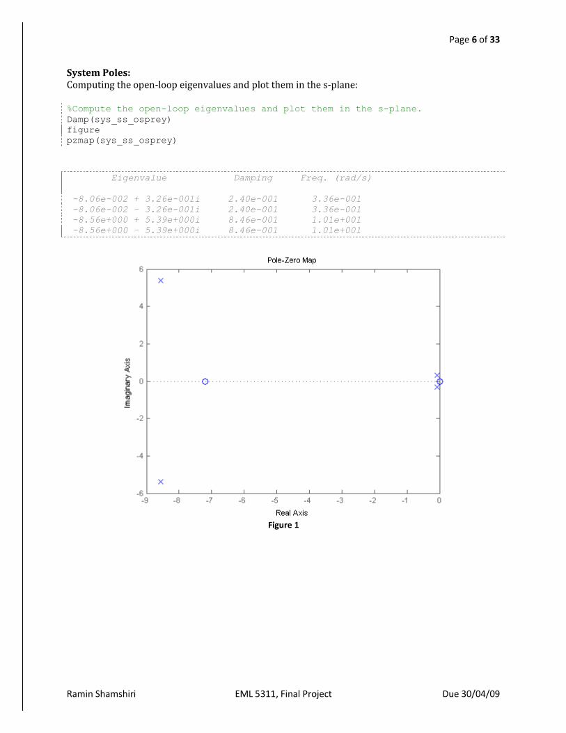
System Poles: Computing the open-loop eigenvalues and plot them in the s-plane: %Compute the open-loop eigenvalues and plot them in the s-plane.
Damp(sys_ss_osprey)
figure
pzmap(sys_ss_osprey)
Eigenvalue Damping Freq. (rad/s)
-8.06e-002 + 3.26e-001i 2.40e-001 3.36e-001
-8.06e-002 – 3.26e-001i 2.40e-001 3.36e-001
-8.56e+000 + 5.39e+000i 8.46e-001 1.01e+001
-8.56e+000 – 5.39e+000i 8.46e-001 1.01e+001
Figure 1
Page 7 of 33
Ramin Shamshiri EML 5311, Final Project Due 30/04/09
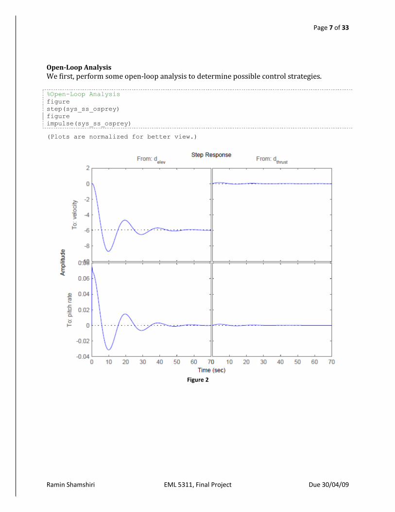
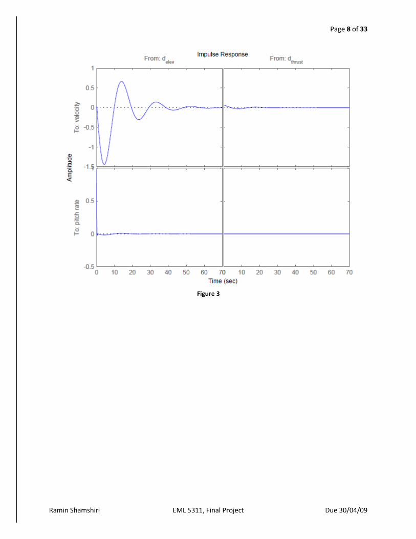
Open-Loop Analysis
We first, perform some open-loop analysis to determine possible control strategies. %Open-Loop Analysis
figure
step(sys_ss_osprey)
figure
impulse(sys_ss_osprey)
(Plots are normalized for better view.)
Figure 2
Page 8 of 33
Ramin Shamshiri EML 5311, Final Project Due 30/04/09
Figure 3

Page 9 of 33
Ramin Shamshiri EML 5311, Final Project Due 30/04/09
Selecting TF21 , 𝑶𝒖𝒕𝒑𝒖𝒕𝟐
𝑰𝒏𝒑𝒖𝒕𝟏 : pitch rate to elevator
% Select I/O pair:
sys21_ss=sys_ss_osprey('Pitch rate','d_{elev}')
sys21_tf=sys_tf_osprey(2,1)
% Bode Plot
figure
bode(sys21_ss)
a =
Velocity Angle of att Pitch rate Pitch Angle
Velocity -0.147 11.08 0.0841 -9.806
Angle of att -0.0316 -7.171 0.8281 0
Pitch rate 0 -37.35 -9.963 0
Pitch Angle 0 0 1 0
b =
d_{elev}
Velocity 0.03357
Angle of att 1e-005
Pitch rate 0.98
Pitch Angle 0
c =
Velocity Angle of att Pitch rate Pitch Angle
pitch rate 0 0 1 0
d =
d_{elev}
pitch rate 0
Continuous-time model.
𝑃𝑖𝑡𝑐ℎ 𝑟𝑎𝑡𝑒
𝐸𝑙𝑒𝑣𝑎𝑡𝑜𝑟=
0.98 𝑠3 + 7.171 𝑠2 + 1.416 𝑠
𝑠4 + 17.28 𝑠3 + 105.2 𝑠2 + 18.44 𝑠 + 11.58

Page 10 of 33
Ramin Shamshiri EML 5311, Final Project Due 30/04/09

Page 11 of 33
Ramin Shamshiri EML 5311, Final Project Due 30/04/09
Root Locus Design

Page 12 of 33
Ramin Shamshiri EML 5311, Final Project Due 30/04/09
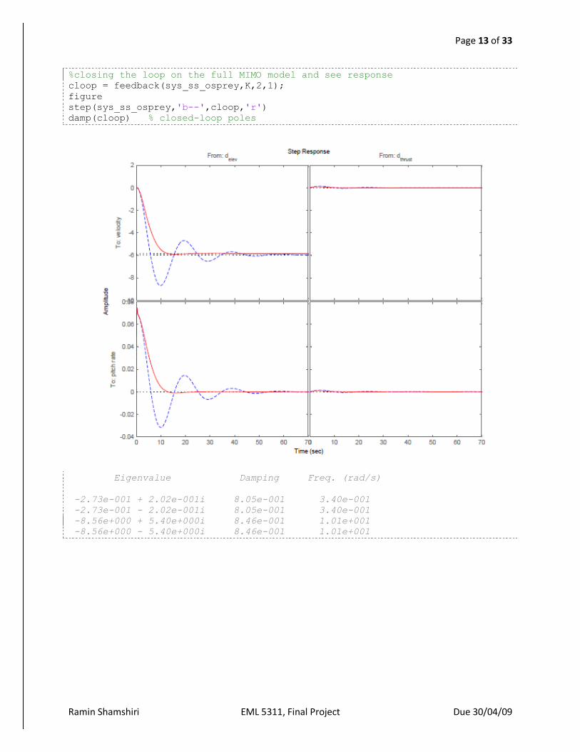
Closing the SISO feedback loop and plotting the closed loop step response and compare it to the open loop step response: %close the SISO feedback loop.
K = 6.42;
cl21 = feedback(sys21,K);
%Plot the closed-loop step response, and compare it to the open-loop step
response.
figure
step(sys21,'b--',cl21,'r')
Page 13 of 33
Ramin Shamshiri EML 5311, Final Project Due 30/04/09
%closing the loop on the full MIMO model and see response
cloop = feedback(sys_ss_osprey,K,2,1);
figure
step(sys_ss_osprey,'b--',cloop,'r')
damp(cloop) % closed-loop poles
Eigenvalue Damping Freq. (rad/s)
-2.73e-001 + 2.02e-001i 8.05e-001 3.40e-001
-2.73e-001 - 2.02e-001i 8.05e-001 3.40e-001
-8.56e+000 + 5.40e+000i 8.46e-001 1.01e+001
-8.56e+000 - 5.40e+000i 8.46e-001 1.01e+001
Page 14 of 33
Ramin Shamshiri EML 5311, Final Project Due 30/04/09
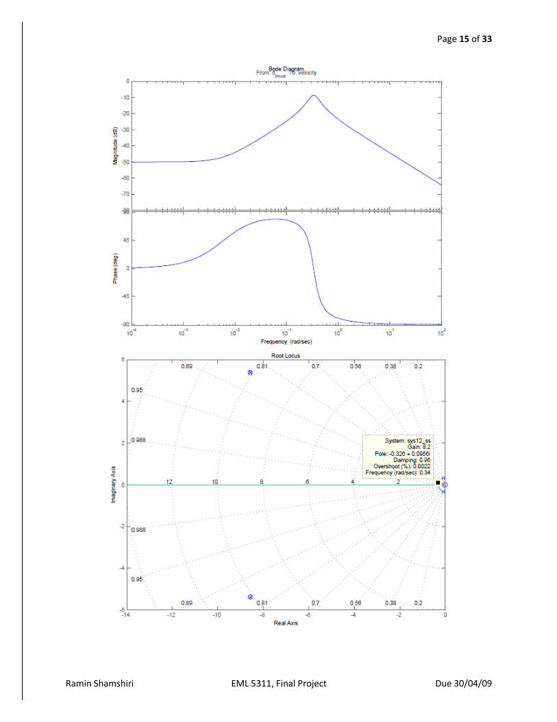
TF12 , 𝑶𝒖𝒕𝒑𝒖𝒕𝟏
𝑰𝒏𝒑𝒖𝒕𝟐 : velocity rate to thrust
% Select I/O pair: sys12_ss=d_{thrust} to output velocity
sys12_ss=sys_ss_osprey('velocity','d_{thrust}')
sys12_tf=sys_tf_osprey(1,2)
% Bode Plot for ss12
figure
bode(sys12_ss)
% Plot the root locus for ss12
figure
rlocus(sys12_ss)
sgrid
%close the SISO feedback loop.
K_12 = 8.67;
cl21 = feedback(sys12_ss,K_12);
%Plot the closed-loop step response, and compare it to the open-loop step
response.
figure
step(sys12_ss,'b--',cl21,'r')
%closing the loop on the full MIMO model and see response
cloop = feedback(sys_ss_osprey,K_12,2,1);
figure
step(sys_ss_osprey,'b--',cloop,'r')
damp(cloop) % closed-loop poles
a =
Velocity Angle of att Pitch rate Pitch Angle
Velocity -0.147 11.08 0.0841 -9.806
Angle of att -0.0316 -7.171 0.8281 0
Pitch rate 0 -37.35 -9.963 0
Pitch Angle 0 0 1 0
b =
d_{thrust}
Velocity 0.06
Angle of att 0.0001
Pitch rate 0
Pitch Angle 0
c =
Velocity Angle of att Pitch rate Pitch Angle
velocity 1 0 0 0
d =
d_{thrust}
velocity 0
Continuous-time model.
Transfer function from input "d_{thrust}" to output "velocity":
0.06 s^3 + 1.029 s^2 + 6.153 s + 0.03663
---------------------------------------------
s^4 + 17.28 s^3 + 105.2 s^2 + 18.44 s + 11.58
Page 15 of 33
Ramin Shamshiri EML 5311, Final Project Due 30/04/09

Page 16 of 33
Ramin Shamshiri EML 5311, Final Project Due 30/04/09

Page 17 of 33
Ramin Shamshiri EML 5311, Final Project Due 30/04/09
Eigenvalue Damping Freq. (rad/s)
-3.35e-001 1.00e+000 3.35e-001
-3.47e-001 1.00e+000 3.47e-001
-8.56e+000 + 5.40e+000i 8.46e-001 1.01e+001
-8.56e+000 - 5.40e+000i 8.46e-001 1.01e+001
Page 18 of 33
Ramin Shamshiri EML 5311, Final Project Due 30/04/09
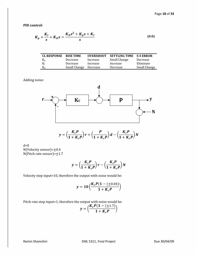
PID control:
𝑲𝒑 +𝑲𝑰
𝒔+ 𝑲𝑫𝒔 =
𝑲𝑫𝒔𝟐 + 𝑲𝒑𝒔 + 𝑲𝑰
𝒔 (0.0)
CL RESPONSE RISE TIME OVERSHOOT SETTLING TIME S-S ERROR Kp Decrease Increase Small Change Decrease KI Decrease Increase Increase Eliminate Kd Small Change Decrease Decrease Small Change
Adding noise:
𝒚 = 𝑲𝒄𝑷
𝟏 + 𝑲𝒄𝑷 𝒓 +
𝑷
𝟏 + 𝑲𝒄𝑷 𝒅 −
𝑲𝒄𝑷
𝟏 + 𝑲𝒄𝑷 𝑵
d=0 N(Velocity sensor)=±0.4 N(Pitch rate sensor)=±1.7
𝒚 = 𝑲𝒄𝑷
𝟏 + 𝑲𝒄𝑷 𝒓 −
𝑲𝒄𝑷
𝟏 + 𝑲𝒄𝑷 𝑵
Velocity step input=10, therefore the output with noise would be:
𝒚 = 𝟏𝟎 𝑲𝒄𝑷(𝟏 − (±0.04)
𝟏 + 𝑲𝒄𝑷
Pitch rate step input=1, therefore the output with noise would be:
𝒚 = 𝑲𝒄𝑷(𝟏 − (±1.7)
𝟏 + 𝑲𝒄𝑷

Page 19 of 33
Ramin Shamshiri EML 5311, Final Project Due 30/04/09
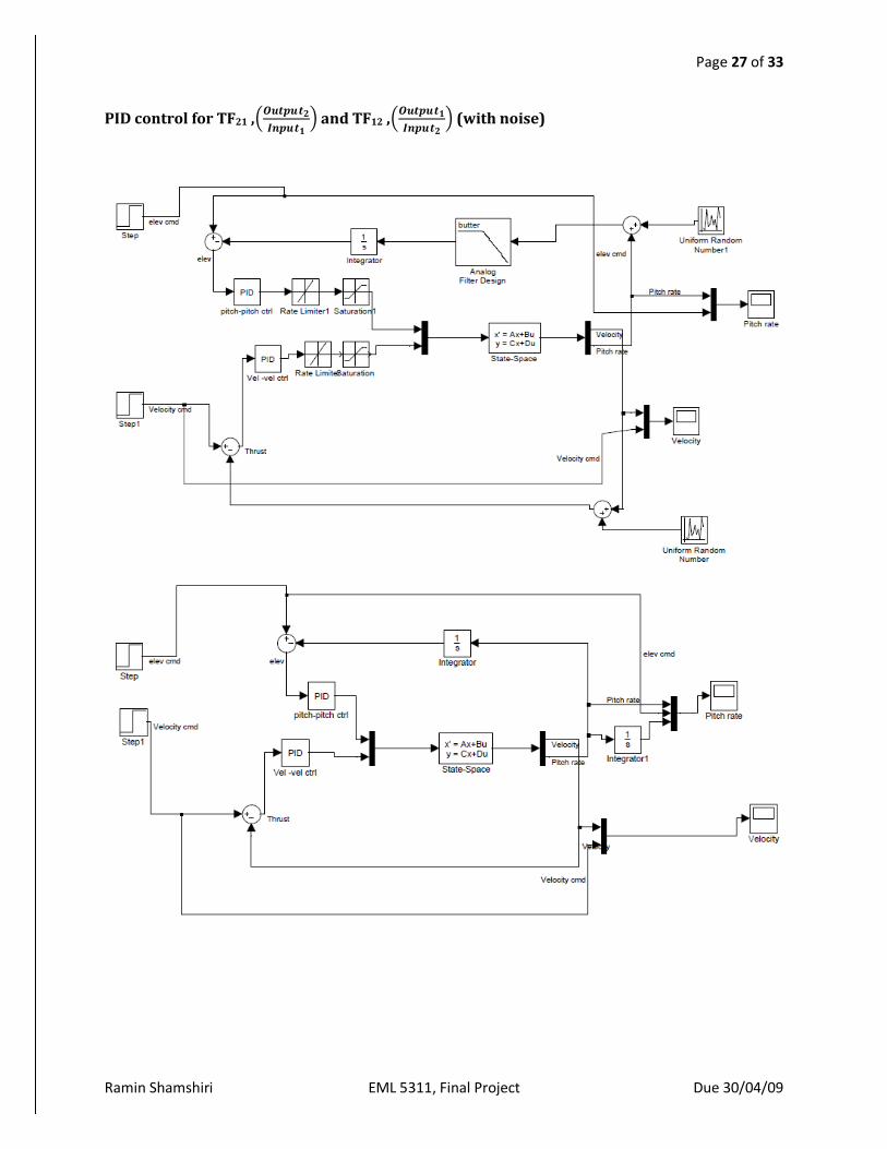
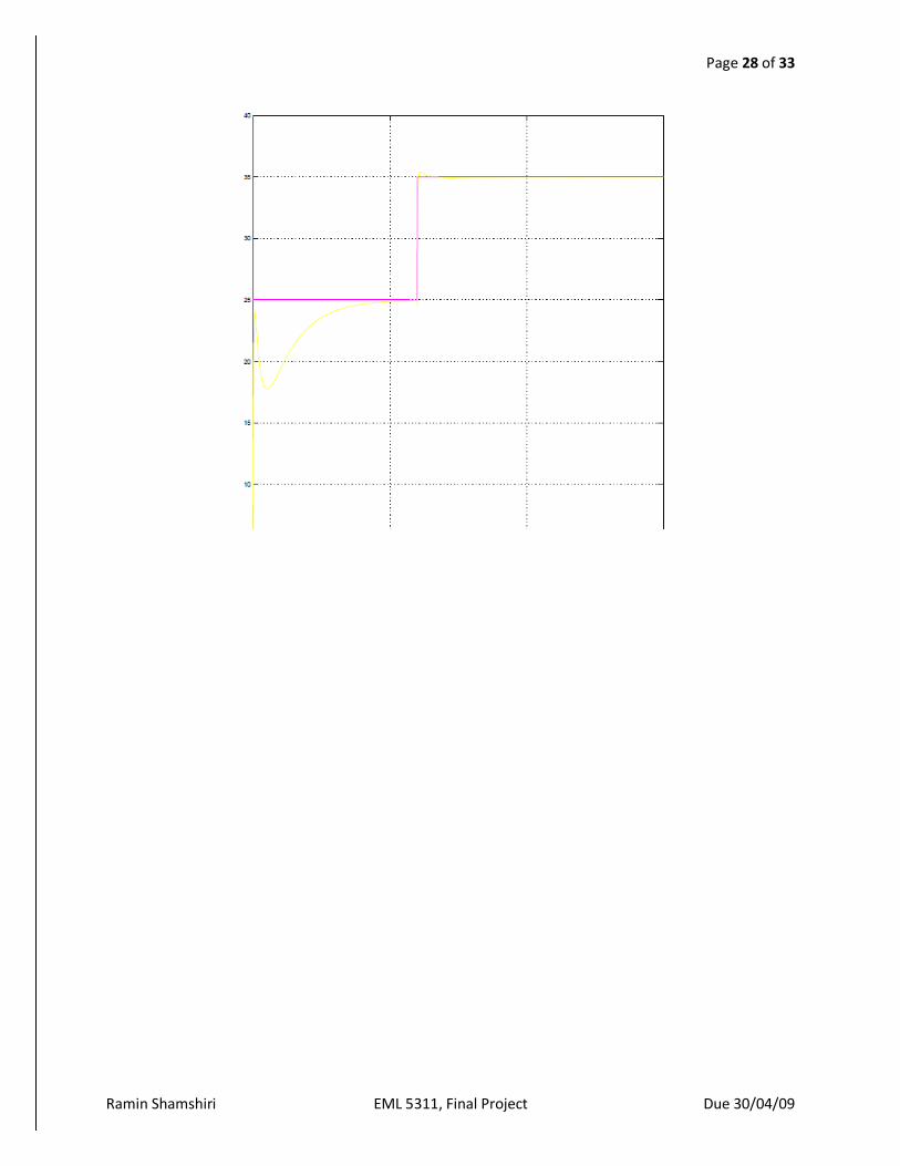
PID control for TF21 , 𝑶𝒖𝒕𝒑𝒖𝒕𝟐
𝑰𝒏𝒑𝒖𝒕𝟏 : pitch rate to elevator (without noise)
𝑃𝑖𝑡𝑐ℎ 𝑟𝑎𝑡𝑒
𝐸𝑙𝑒𝑣𝑎𝑡𝑜𝑟=
0.98 𝑠3 + 7.171 𝑠2 + 1.416 𝑠
𝑠4 + 17.28 𝑠3 + 105.2 𝑠2 + 18.44 𝑠 + 11.58
% TF21: (Output2/Input1); pitch rate to elevator
sys21_tf=sys_tf_osprey(2,1);
num_sys21_tf=[0.98,7.171,1.416,0];
den_sys21_tf=[1,17.28,105.2,18.44,11.58];
%Ploting Open Loop step response for TF21:
figure
step(sys21_tf)
%Results:

Page 20 of 33
Ramin Shamshiri EML 5311, Final Project Due 30/04/09
%Close loop reponse:
%P control for TF_21
Kp_21=.5;% Proportional gain
num_Kp_21=[Kp_21];%P TF num
den_Kp_21=[1];%P TF denum
num_P_21=conv(num_Kp_21,num_sys21_tf);
den_P_21=conv(den_Kp_21,den_sys21_tf);
[num_P_Control_21,den_P_Control_21]=cloop(num_P_21,den_P_21);
sys_tf_P_21=tf(num_P_Control_21,den_P_Control_21)
%Plotting P control reponse and comparing it with open loop step response
figure
step(sys21_tf,'b--',sys_tf_P_21,'r')
%Results:
Page 21 of 33
Ramin Shamshiri EML 5311, Final Project Due 30/04/09
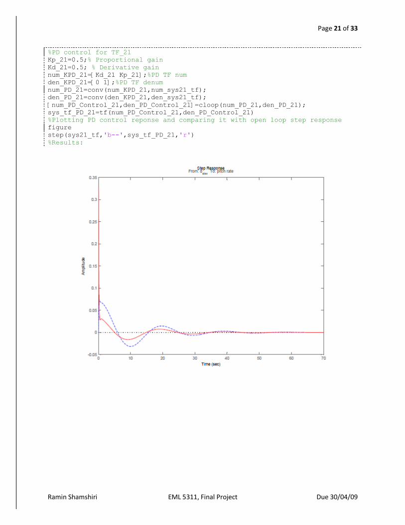
%PD control for TF_21
Kp_21=0.5;% Proportional gain
Kd_21=0.5; % Derivative gain
num_KPD_21=[Kd_21 Kp_21];%PD TF num
den_KPD_21=[0 1];%PD TF denum
num_PD_21=conv(num_KPD_21,num_sys21_tf);
den_PD_21=conv(den_KPD_21,den_sys21_tf);
[num_PD_Control_21,den_PD_Control_21]=cloop(num_PD_21,den_PD_21);
sys_tf_PD_21=tf(num_PD_Control_21,den_PD_Control_21)
%Plotting PD control reponse and comparing it with open loop step response
figure
step(sys21_tf,'b--',sys_tf_PD_21,'r')
%Results:

Page 22 of 33
Ramin Shamshiri EML 5311, Final Project Due 30/04/09
%PID control for TF_21
Kp_21=100;% Proportional gain
Kd_21=1; % Derivative gain
Ki_21=200;% Integral gain
num_KPID_21=[Kd_21 Kp_21 Ki_21];%PID TF num
den_KPID_21=[1 0];%PID TF denum
num_PID_21=conv(num_KPID_21,num_sys21_tf);
den_PID_21=conv(den_KPID_21,den_sys21_tf);
[num_PID_Control_21,den_PID_Control_21]=cloop(num_PID_21,den_PID_21);
sys_tf_PID_21=tf(num_PID_Control_21,den_PID_Control_21)
%Plotting PD control reponse:
figure
step(sys21_tf,'b--',sys_tf_PID_21,'r')

Page 23 of 33
Ramin Shamshiri EML 5311, Final Project Due 30/04/09
PID control for TF12 , 𝑶𝒖𝒕𝒑𝒖𝒕𝟏
𝑰𝒏𝒑𝒖𝒕𝟐 : velocity rate to thrust, (without noise)
𝑃𝑖𝑡𝑐ℎ 𝑟𝑎𝑡𝑒
𝐸𝑙𝑒𝑣𝑎𝑡𝑜𝑟=
0.06 𝑠3 + 1.029 𝑠2 + 6.153 𝑠 + 0.03663
𝑠4 + 17.28 𝑠3 + 105.2 𝑠2 + 18.44 𝑠 + 11.58
% TF12: (Output1/Input2); d_{thrust} to output velocity:
sys12_tf=sys_tf_osprey(1,2);
num_sys12_tf=[0.06,1.029,6.153,0.03663];
den_sys12_tf=[1,17.28,105.2,18.44,11.58];
%Ploting Open Loop step response for TF12:
figure
step(sys12_tf)

Page 24 of 33
Ramin Shamshiri EML 5311, Final Project Due 30/04/09
%Close loop reponse:
%P control for TF_12
Kp_12=6.5;% Proportional gain
num_Kp_12=[Kp_12];%P TF num
den_Kp_12=[1];%P TF denum
num_P_12=conv(num_Kp_12,num_sys12_tf);
den_P_12=conv(den_Kp_12,den_sys12_tf);
[num_P_Control_12,den_P_Control_12]=cloop(num_P_12,den_P_12);
sys_tf_P_12=tf(num_P_Control_12,den_P_Control_12)
%Plotting P control reponse and comparing it with open loop step response
figure
step(sys12_tf,'b--',sys_tf_P_12,'r')
%Results:

Page 25 of 33
Ramin Shamshiri EML 5311, Final Project Due 30/04/09
%PD control for TF_12
Kp_12=1;% Proportional gain
Kd_12=1; % Derivative gain
num_KPD_12=[Kd_12 Kp_12];%PD TF num
den_KPD_12=[0 1];%PD TF denum
num_PD_12=conv(num_KPD_12,num_sys12_tf);
den_PD_12=conv(den_KPD_12,den_sys12_tf);
[num_PD_Control_12,den_PD_Control_12]=cloop(num_PD_12,den_PD_12);
sys_tf_PD_12=tf(num_PD_Control_12,den_PD_Control_12)
%Plotting PD control reponse and comparing it with open loop step response
figure
step(sys12_tf,'b--',sys_tf_PD_12,'r')
%Results:
Page 26 of 33
Ramin Shamshiri EML 5311, Final Project Due 30/04/09
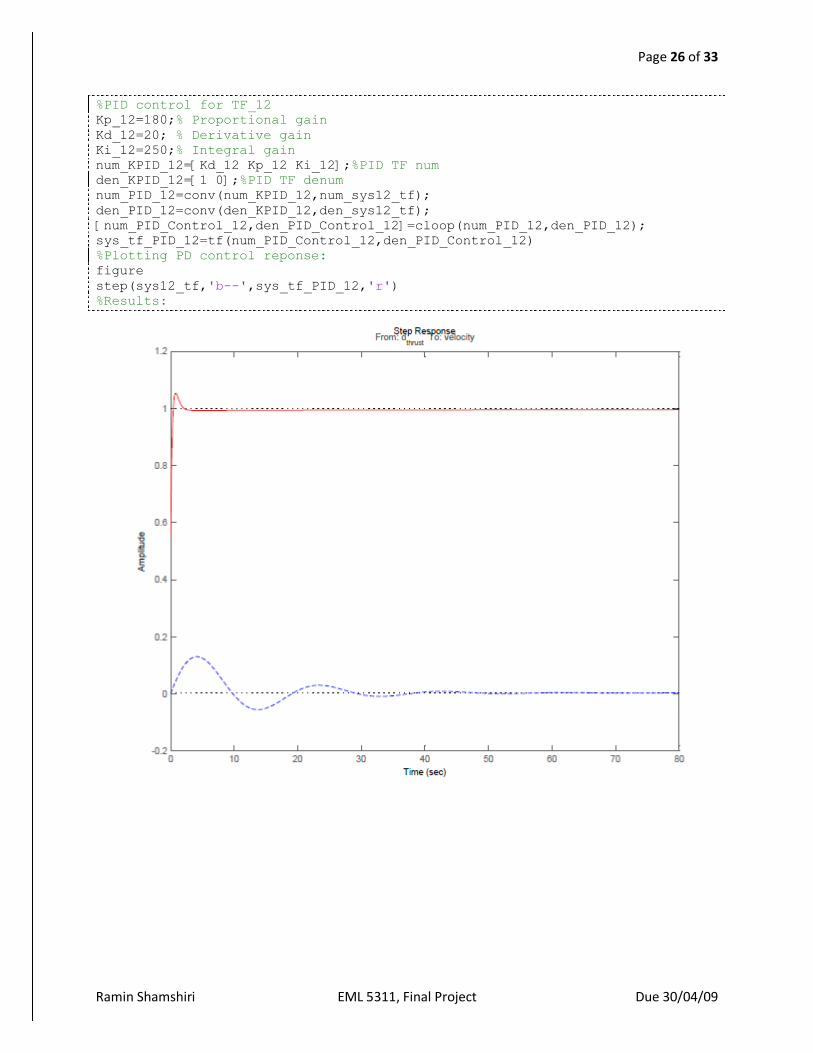
%PID control for TF_12
Kp_12=180;% Proportional gain
Kd_12=20; % Derivative gain
Ki_12=250;% Integral gain
num_KPID_12=[Kd_12 Kp_12 Ki_12];%PID TF num
den_KPID_12=[1 0];%PID TF denum
num_PID_12=conv(num_KPID_12,num_sys12_tf);
den_PID_12=conv(den_KPID_12,den_sys12_tf);
[num_PID_Control_12,den_PID_Control_12]=cloop(num_PID_12,den_PID_12);
sys_tf_PID_12=tf(num_PID_Control_12,den_PID_Control_12)
%Plotting PD control reponse:
figure
step(sys12_tf,'b--',sys_tf_PID_12,'r')
%Results:
Page 27 of 33
Ramin Shamshiri EML 5311, Final Project Due 30/04/09
PID control for TF21 , 𝑶𝒖𝒕𝒑𝒖𝒕𝟐
𝑰𝒏𝒑𝒖𝒕𝟏 and TF12 ,
𝑶𝒖𝒕𝒑𝒖𝒕𝟏
𝑰𝒏𝒑𝒖𝒕𝟐 (with noise)
Page 28 of 33
Ramin Shamshiri EML 5311, Final Project Due 30/04/09

Page 29 of 33
Ramin Shamshiri EML 5311, Final Project Due 30/04/09
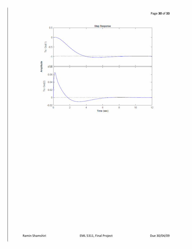
LQR Controller 𝑲 = 𝑹−𝟏𝑩𝑻𝑺
𝒖 = −𝑲𝒙 where S comes from ARE solution and R=I2x2
%LQR design with C=I(4X4)
A=[-0.1470 11.0767 0.0841 -9.8065;-0.0316 -7.1712 0.8281 0;0 -37.3527 -9.9628
0;0 0 1 0];
B=[3.1^-3 0.06;10^-5 10^-4;0.98 0;0 0];
C=[1 0 0 0;0 0 1 0];
D=[0 0;0 0];
Q=eye(4)'*eye(4);R=eye(2);
%Checking Controllability and Observability
CO=ctrb(A,B);% Check Controllability
OB=obsv(A,C); % Check Observability
Controllability=rank(CO); Observability=rank(OB);
[sqrt(Q);sqrt(Q)*A;sqrt(Q)*(A^2);sqrt(Q)*(A^3)];
%Conclusion:
%completely state controllable
%completey state observable
[K_1,S,E]=lqr(A,B,Q,R)
%u=-Kx
Ac = [(A-B*K_1)];
Bc = [B];
Cc = [C];
Dc = [0 0;0 0];
figure
step(Ac,Bc,Cc,Dc,1)
K_1 =
-0.5658 -5.6563 0.9999 14.6650
0.0791 0.2774 -0.0379 -0.6654
S =
1.3101 4.5643 -0.6223 -10.9368
4.5643 35.7631 -5.9284 -91.4425
-0.6223 -5.9284 1.0416 15.3398
-10.9368 -91.4425 15.3398 238.0566
E =
-8.5808 + 5.3836i
-8.5808 - 5.3836i
-0.5425 + 0.6219i
-0.5425 - 0.6219i
Page 30 of 33
Ramin Shamshiri EML 5311, Final Project Due 30/04/09

Page 31 of 33
Ramin Shamshiri EML 5311, Final Project Due 30/04/09
LQR Controller plus observer %LQR design with C as in dynamic model
Q=C'*C;
%Checking Controllability and Observability
rank([sqrt(Q);sqrt(Q)*A;sqrt(Q)*(A^2);sqrt(Q)*(A^3)]);
[K,S,E]=lqr(A,B,Q,R)
Ac = [(A-B*K)];
Bc = [B];
Cc = [C];
Dc = [0 0;0 0];
figure
step(Ac,Bc,Cc,Dc,1)
%Observer design
% Finding controller poles
poles = eig(Ac)
P = [-5 -6 -7 -8];
L = place(A',C',P)';
Ace = [A-B*K B*K;
zeros(size(A)) (A-L*C)];
Bce = [ B;
zeros(size(B))];
Cce = [Cc zeros(size(Cc))];
Dce = [0 0;0 0];
t=0:0.01:12;
figure
step(Ace,Bce,Cce,Dce,1,t);
poles =
-8.5807 + 5.3833i
-8.5807 - 5.3833i
-0.5414 + 0.6228i
-0.5414 - 0.6228i

Page 32 of 33
Ramin Shamshiri EML 5311, Final Project Due 30/04/09

Page 33 of 33
Ramin Shamshiri EML 5311, Final Project Due 30/04/09
Report:
Two separate PID controllers were designed for two of the four transfer functions of this MIMO system. The first transfer function TF21 link pitch rate to elevator and the second one, TF12 links velocity rate to thrust. Root locus was used to pick the gains for PID and the response are shown in the following figures. Velocity sensor noise and pitch rate sensor noise was implemented in the simulation process. It can be seen that PID control is not an optimum solution for this MIMO problem. To enhance the result, LQR design was used and the corresponding gain matrix was K_1 =
-0.5658 -5.6563 0.9999 14.6650
0.0791 0.2774 -0.0379 -0.6654