Embed Size (px)
Citation preview
EOSC433: Geotechnical Engineering Practice – Limit Equilibrium Lab Exercise
Lab Practical - Limit Equilibrium Analysis of Engineered Slopes Part 1: Planar Analysis A – Deterministic Analysis This exercise will demonstrate the basics of a deterministic limit equilibrium planar analysis using the Rocscience program RocPlane. 1) To begin, start the program RocPlane and create a new model:
Select: File → New
A planar wedge will immediately appear on your screen showing the Top, Front and Side views (i.e. viewing angles differ by 90 degrees).
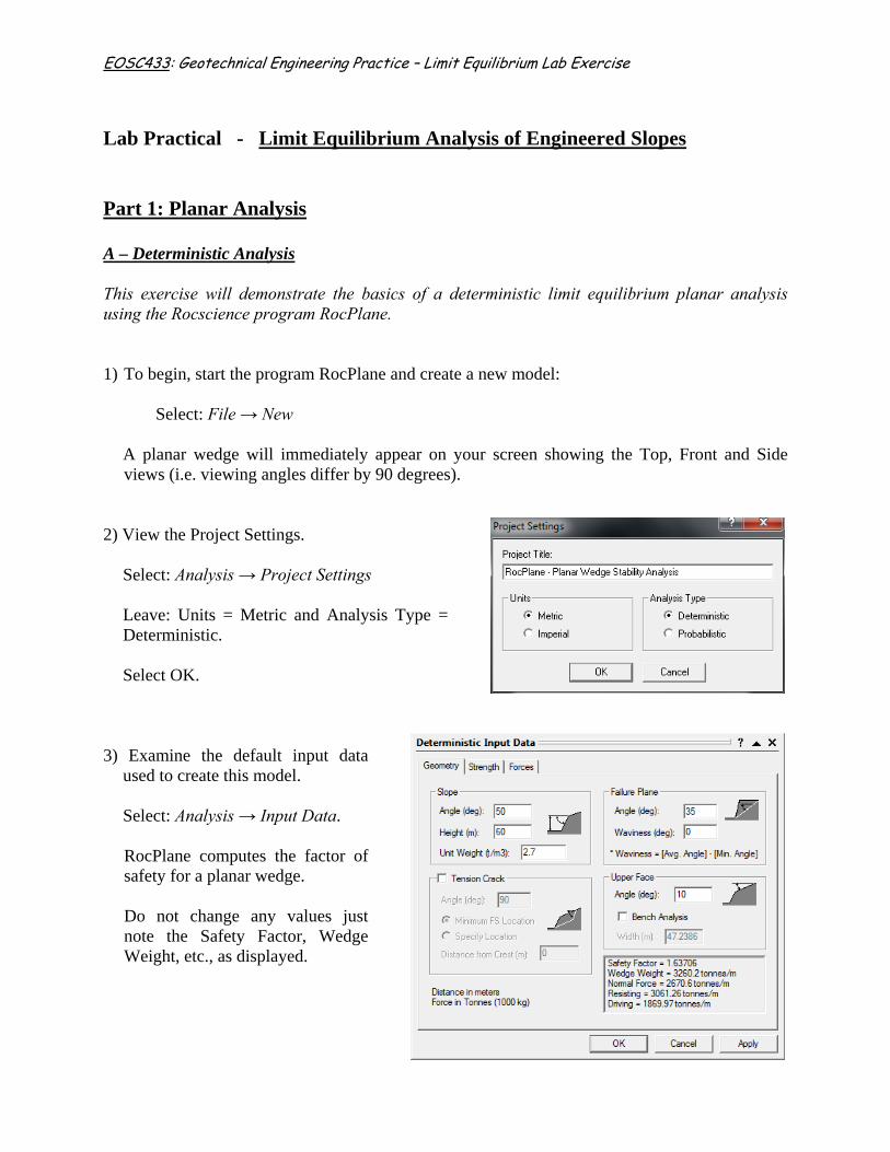
2) View the Project Settings.
Select: Analysis → Project Settings Leave: Units = Metric and Analysis Type = Deterministic. Select OK.
3) Examine the default input data
used to create this model. Select: Analysis → Input Data.
RocPlane computes the factor of safety for a planar wedge. Do not change any values just note the Safety Factor, Wedge Weight, etc., as displayed.
EOSC433: Geotechnical Engineering Practice – Limit Equilibrium Lab Exercise
2
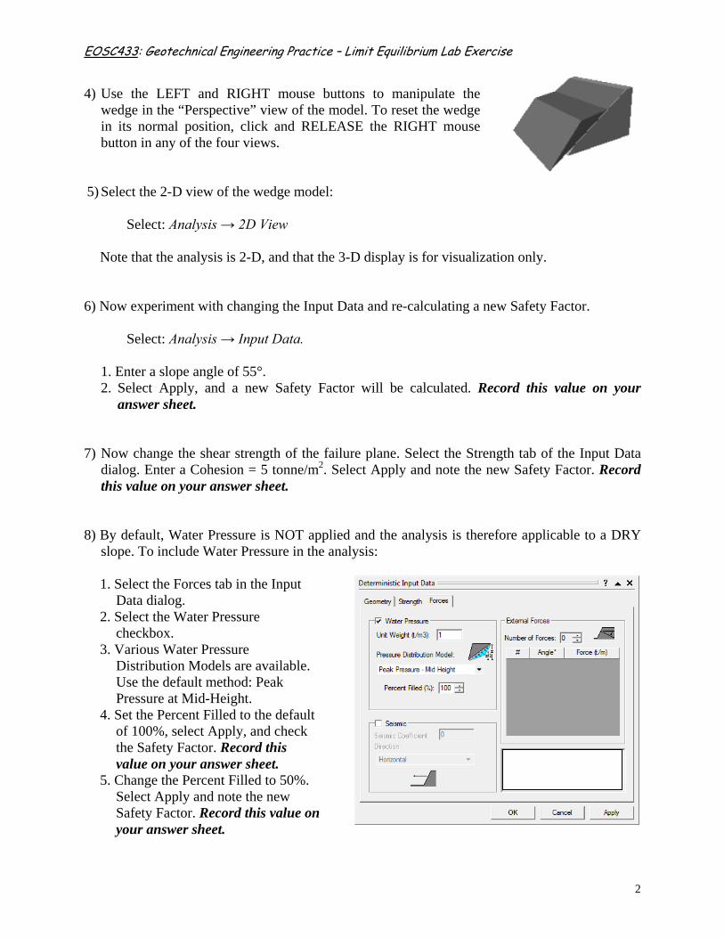
4) Use the LEFT and RIGHT mouse buttons to manipulate the wedge in the “Perspective” view of the model. To reset the wedge in its normal position, click and RELEASE the RIGHT mouse button in any of the four views.
5) Select the 2-D view of the wedge model:
Select: Analysis → 2D View
Note that the analysis is 2-D, and that the 3-D display is for visualization only. 6) Now experiment with changing the Input Data and re-calculating a new Safety Factor.
Select: Analysis → Input Data.
1. Enter a slope angle of 55°. 2. Select Apply, and a new Safety Factor will be calculated. Record this value on your
answer sheet.
7) Now change the shear strength of the failure plane. Select the Strength tab of the Input Data
dialog. Enter a Cohesion = 5 tonne/m2. Select Apply and note the new Safety Factor. Record this value on your answer sheet.
8) By default, Water Pressure is NOT applied and the analysis is therefore applicable to a DRY
slope. To include Water Pressure in the analysis:
1. Select the Forces tab in the Input Data dialog.
2. Select the Water Pressure checkbox.
3. Various Water Pressure Distribution Models are available. Use the default method: Peak Pressure at Mid-Height.
4. Set the Percent Filled to the default of 100%, select Apply, and check the Safety Factor. Record this value on your answer sheet.
5. Change the Percent Filled to 50%. Select Apply and note the new Safety Factor. Record this value on your answer sheet.
EOSC433: Geotechnical Engineering Practice – Limit Equilibrium Lab Exercise
3
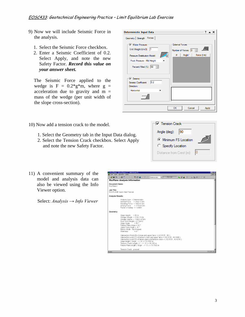
9) Now we will include Seismic Force in the analysis.
1. Select the Seismic Force checkbox. 2. Enter a Seismic Coefficient of 0.2.
Select Apply, and note the new Safety Factor. Record this value on your answer sheet.
The Seismic Force applied to the wedge is F = 0.2*g*m, where g = acceleration due to gravity and m = mass of the wedge (per unit width of the slope cross-section).
10) Now add a tension crack to the model.
1. Select the Geometry tab in the Input Data dialog. 2. Select the Tension Crack checkbox. Select Apply
and note the new Safety Factor.
11) A convenient summary of the
model and analysis data can also be viewed using the Info Viewer option.
Select: Analysis → Info Viewer
EOSC433: Geotechnical Engineering Practice – Limit Equilibrium Lab Exercise
4
B – Sensitivity Analysis
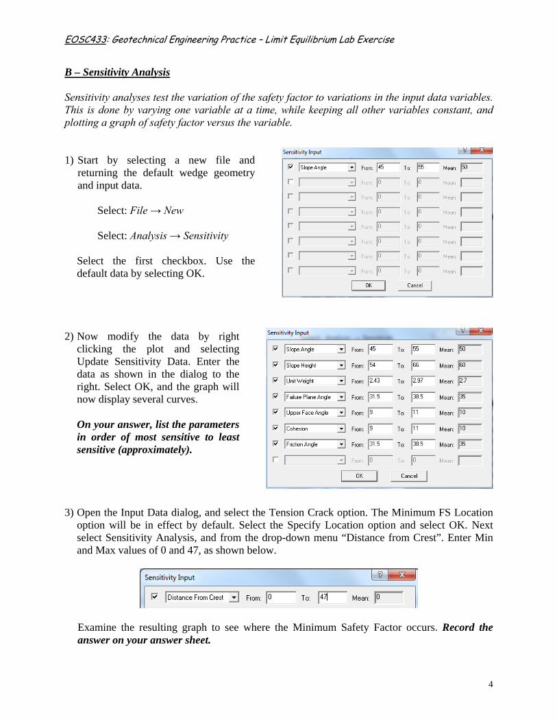
Sensitivity analyses test the variation of the safety factor to variations in the input data variables. This is done by varying one variable at a time, while keeping all other variables constant, and plotting a graph of safety factor versus the variable. 1) Start by selecting a new file and
returning the default wedge geometry and input data.
Select: File → New
Select: Analysis → Sensitivity
Select the first checkbox. Use the default data by selecting OK.
2) Now modify the data by right
clicking the plot and selecting Update Sensitivity Data. Enter the data as shown in the dialog to the right. Select OK, and the graph will now display several curves.
On your answer, list the parameters in order of most sensitive to least sensitive (approximately).
3) Open the Input Data dialog, and select the Tension Crack option. The Minimum FS Location
option will be in effect by default. Select the Specify Location option and select OK. Next select Sensitivity Analysis, and from the drop-down menu “Distance from Crest”. Enter Min and Max values of 0 and 47, as shown below.
Examine the resulting graph to see where the Minimum Safety Factor occurs. Record the answer on your answer sheet.
EOSC433: Geotechnical Engineering Practice – Limit Equilibrium Lab Exercise
5
C – Probabilistic Analysis This tutorial will examine how a Probabilistic analysis is carried out. 1) Begin by creating a new model. The default wedge model will immediately appear on your
screen.
Select: File → New
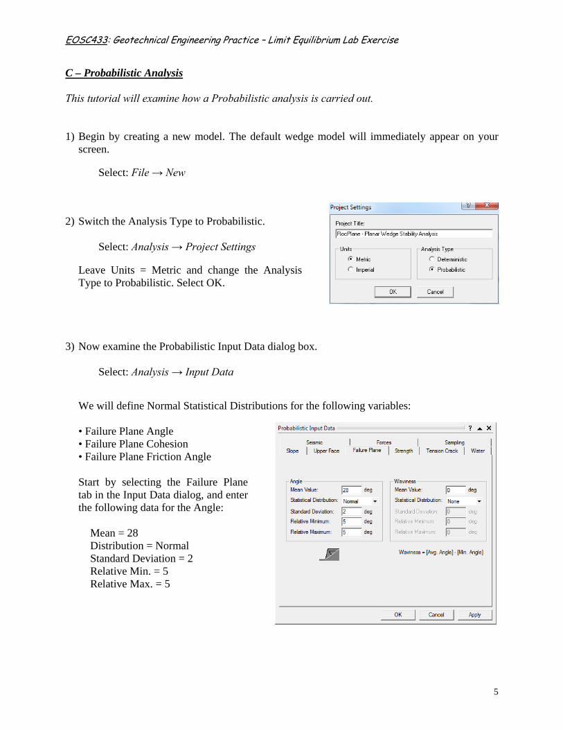
2) Switch the Analysis Type to Probabilistic.
Select: Analysis → Project Settings
Leave Units = Metric and change the Analysis Type to Probabilistic. Select OK.
3) Now examine the Probabilistic Input Data dialog box.
Select: Analysis → Input Data We will define Normal Statistical Distributions for the following variables: • Failure Plane Angle • Failure Plane Cohesion • Failure Plane Friction Angle Start by selecting the Failure Plane tab in the Input Data dialog, and enter the following data for the Angle:
Mean = 28 Distribution = Normal Standard Deviation = 2 Relative Min. = 5 Relative Max. = 5
EOSC433: Geotechnical Engineering Practice – Limit Equilibrium Lab Exercise
6
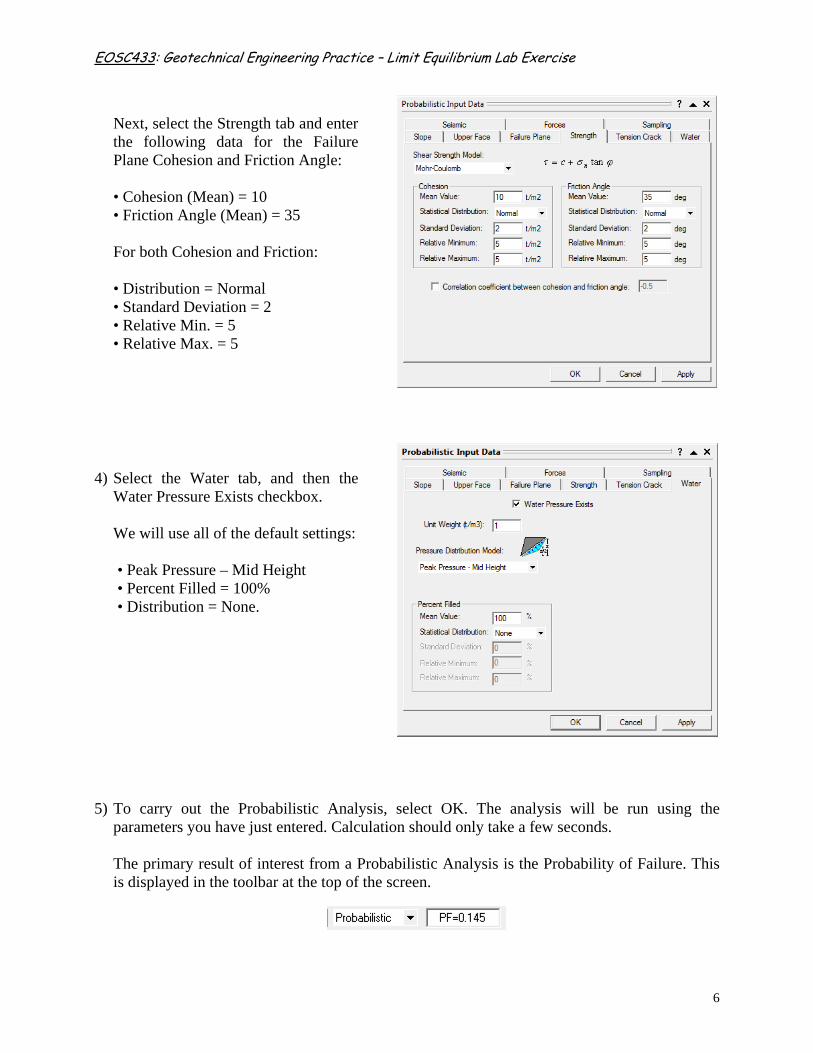
Next, select the Strength tab and enter the following data for the Failure Plane Cohesion and Friction Angle: • Cohesion (Mean) = 10 • Friction Angle (Mean) = 35 For both Cohesion and Friction: • Distribution = Normal • Standard Deviation = 2 • Relative Min. = 5 • Relative Max. = 5
4) Select the Water tab, and then the Water Pressure Exists checkbox.
We will use all of the default settings: • Peak Pressure – Mid Height • Percent Filled = 100% • Distribution = None.
5) To carry out the Probabilistic Analysis, select OK. The analysis will be run using the
parameters you have just entered. Calculation should only take a few seconds.
The primary result of interest from a Probabilistic Analysis is the Probability of Failure. This is displayed in the toolbar at the top of the screen.
EOSC433: Geotechnical Engineering Practice – Limit Equilibrium Lab Exercise
7
A Probability of Failure of PF = 0.145 means 14.5% Probability of Failure. Note that because the Input Data is based on the random generation of numbers (i.e. a Monte Carlo analysis), the Probability of Failure will not necessarily be the same each time you compute with the same data.
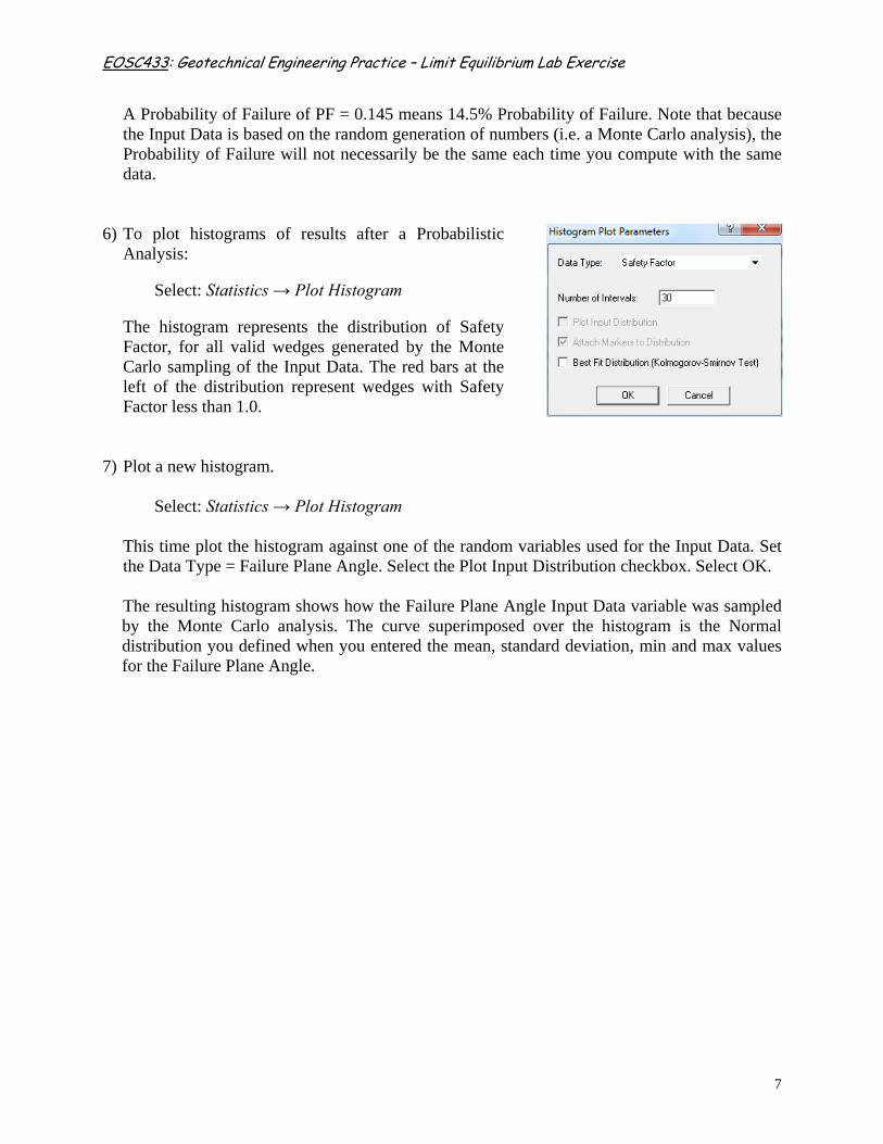
6) To plot histograms of results after a Probabilistic Analysis:
Select: Statistics → Plot Histogram
The histogram represents the distribution of Safety Factor, for all valid wedges generated by the Monte Carlo sampling of the Input Data. The red bars at the left of the distribution represent wedges with Safety Factor less than 1.0.
7) Plot a new histogram.
Select: Statistics → Plot Histogram This time plot the histogram against one of the random variables used for the Input Data. Set the Data Type = Failure Plane Angle. Select the Plot Input Distribution checkbox. Select OK. The resulting histogram shows how the Failure Plane Angle Input Data variable was sampled by the Monte Carlo analysis. The curve superimposed over the histogram is the Normal distribution you defined when you entered the mean, standard deviation, min and max values for the Failure Plane Angle.
EOSC433: Geotechnical Engineering Practice – Limit Equilibrium Lab Exercise
8
Lab Practical - Limit Equilibrium Analysis of Engineered Slopes
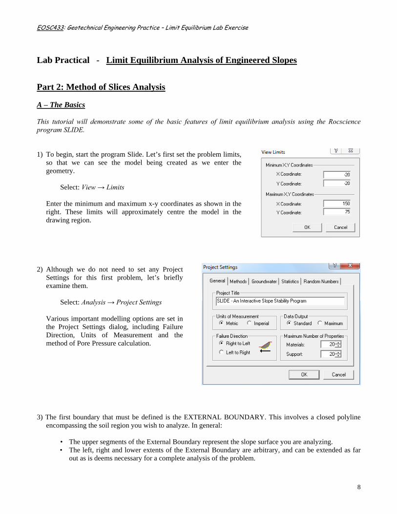
Part 2: Method of Slices Analysis A – The Basics This tutorial will demonstrate some of the basic features of limit equilibrium analysis using the Rocscience program SLIDE. 1) To begin, start the program Slide. Let’s first set the problem limits,
so that we can see the model being created as we enter the geometry.
Select: View → Limits
Enter the minimum and maximum x-y coordinates as shown in the right. These limits will approximately centre the model in the drawing region.
2) Although we do not need to set any Project
Settings for this first problem, let’s briefly examine them.
Select: Analysis → Project Settings
Various important modelling options are set in the Project Settings dialog, including Failure Direction, Units of Measurement and the method of Pore Pressure calculation.
3) The first boundary that must be defined is the EXTERNAL BOUNDARY. This involves a closed polyline
encompassing the soil region you wish to analyze. In general:
• The upper segments of the External Boundary represent the slope surface you are analyzing. • The left, right and lower extents of the External Boundary are arbitrary, and can be extended as far
out as is deems necessary for a complete analysis of the problem.
EOSC433: Geotechnical Engineering Practice – Limit Equilibrium Lab Exercise
9
To add the External Boundary, select Add External Boundary from the Boundaries menu or the Boundaries toolbar.
Select: Boundaries → Add External Boundary
Enter the following coordinates in the prompt line at the bottom right of the screen:
Note that entering c after the last vertex has been entered, automatically connects the first and last vertices (closes the boundary), and exits the Add External Boundary option.
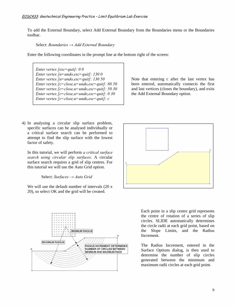
4) In analysing a circular slip surface problem,
specific surfaces can be analysed individually or a critical surface search can be performed to attempt to find the slip surface with the lowest factor of safety.
In this tutorial, we will perform a critical surface search using circular slip surfaces. A circular surface search requires a grid of slip centres. For this tutorial we will use the Auto Grid option.
Select: Surfaces → Auto Grid We will use the default number of intervals (20 x 20), so select OK and the grid will be created.
Each point in a slip centre grid represents the centre of rotation of a series of slip circles. SLIDE automatically determines the circle radii at each grid point, based on the Slope Limits, and the Radius Increment. The Radius Increment, entered in the Surface Options dialog, is then used to determine the number of slip circles generated between the minimum and maximum radii circles at each grid point.
Enter vertex [esc=quit]: 0 0 Enter vertex [u=undo,esc=quit]: 130 0 Enter vertex [u=undo,esc=quit]: 130 50 Enter vertex [c=close,u=undo,esc=quit]: 80 50 Enter vertex [c=close,u=undo,esc=quit]: 50 30 Enter vertex [c=close,u=undo,esc=quit]: 0 30 Enter vertex [c=close,u=undo,esc=quit]: c
EOSC433: Geotechnical Engineering Practice – Limit Equilibrium Lab Exercise
10
When you created the External Boundary, you will also have noticed the two green triangular markers displayed at the left and right limits of the upper surface of the External Boundary. These are the Slope Limits. All slip surfaces must intersect the External Boundary, within the Slope Limits. If the start and end points of a slip surface are NOT within the Slope Limits, then the slip surface is discarded (i.e. not analyzed).
5) Let’s take a look at the Surface Options dialog.
Select: Surfaces → Surface Options
Note:
• The default Surface Type is Circular, which is what we are using for this tutorial.
• The Radius Increment used for the Grid Search is entered in this dialog.
Since we are using the default Surface Options, no changes are required so select Cancel.
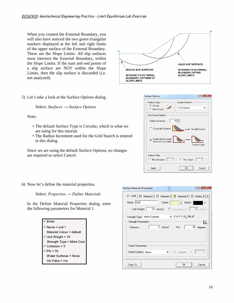
6) Now let’s define the material properties.
Select: Properties → Define Materials
In the Define Material Properties dialog, enter the following parameters for Material 1.
EOSC433: Geotechnical Engineering Practice – Limit Equilibrium Lab Exercise
11
NOTE: Since we are dealing with a single material model, and since you entered properties with the first (default) tab selected, you do not have to assign these properties to the model. SLIDE automatically assigns the default properties (i.e. the properties of the first material in the Define Material Properties dialog) for you. For multiple material models, it is necessary for the user to assign properties with the Assign Properties option.
7) Before we run the analysis, let’s examine the Analysis Methods that are available in SLIDE.
Select: Project Settings → Methods
By default, Bishop and Janbu Simplified limit equilibrium analysis methods are always performed in a SLIDE. In addition to the required methods, the user may choose any or all of the Optional Methods – Spencer, Corps of Engineers (1 & 2), Lowe-Karafiath, and GLE (General Limit Equilibrium).
For this tutorial, we will use the default analysis methods – Bishop and Janbu Simplified, as well as Ordinary/Fellenius, Janbu Corrected and GLE/Morgenstern-Price. Toggle these options on and select OK. We are now finished with the modeling, and can proceed to run the analysis and interpret the results.
8) Before you analyze your model, save it as a file called “quick.sli” (SLIDE model files have a .SLI filename
extension).
Select: File → Save
Use the Save As dialog to save the file. You are now ready to run the analysis.
Select: Analysis → Compute
The SLIDE COMPUTE engine will proceed in running the analysis. This should only take a few seconds. When completed, you are ready to view the results in INTERPRET.
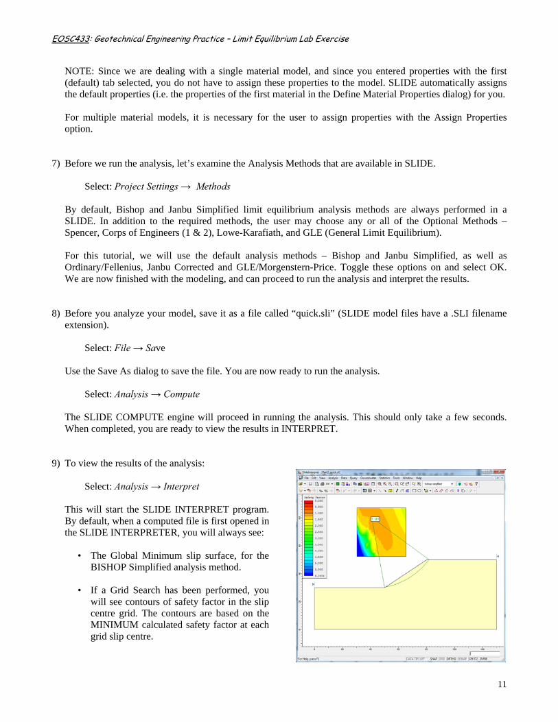
9) To view the results of the analysis:
Select: Analysis → Interpret
This will start the SLIDE INTERPRET program. By default, when a computed file is first opened in the SLIDE INTERPRETER, you will always see:
• The Global Minimum slip surface, for the BISHOP Simplified analysis method.
• If a Grid Search has been performed, you
will see contours of safety factor in the slip centre grid. The contours are based on the MINIMUM calculated safety factor at each grid slip centre.
EOSC433: Geotechnical Engineering Practice – Limit Equilibrium Lab Exercise
12
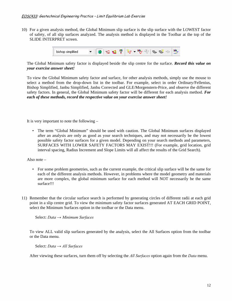
10) For a given analysis method, the Global Minimum slip surface is the slip surface with the LOWEST factor of safety, of all slip surfaces analyzed. The analysis method is displayed in the Toolbar at the top of the SLIDE INTERPRET screen.
The Global Minimum safety factor is displayed beside the slip centre for the surface. Record this value on your exercise answer sheet! To view the Global Minimum safety factor and surface, for other analysis methods, simply use the mouse to select a method from the drop-down list in the toolbar. For example, select in order Ordinary/Fellenius, Bishop Simplified, Janbu Simplified, Janbu Corrected and GLE/Morgenstern-Price, and observe the different safety factors. In general, the Global Minimum safety factor will be different for each analysis method. For each of these methods, record the respective value on your exercise answer sheet!
It is very important to note the following –
• The term “Global Minimum” should be used with caution. The Global Minimum surfaces displayed after an analysis are only as good as your search techniques, and may not necessarily be the lowest possible safety factor surfaces for a given model. Depending on your search methods and parameters, SURFACES WITH LOWER SAFETY FACTORS MAY EXIST!!! (For example, grid location, grid interval spacing, Radius Increment and Slope Limits will all affect the results of the Grid Search).
Also note –
• For some problem geometries, such as the current example, the critical slip surface will be the same for
each of the different analysis methods. However, in problems where the model geometry and materials are more complex, the global minimum surface for each method will NOT necessarily be the same surface!!!
11) Remember that the circular surface search is performed by generating circles of different radii at each grid
point in a slip centre grid. To view the minimum safety factor surfaces generated AT EACH GRID POINT, select the Minimum Surfaces option in the toolbar or the Data menu.
Select: Data → Minimum Surfaces
To view ALL valid slip surfaces generated by the analysis, select the All Surfaces option from the toolbar or the Data menu.
Select: Data → All Surfaces
After viewing these surfaces, turn them off by selecting the All Surfaces option again from the Data menu.
EOSC433: Geotechnical Engineering Practice – Limit Equilibrium Lab Exercise
13
12) The Info Viewer option in the Analysis menu (and the Standard toolbar) displays a summary of SLIDE model parameters, as well as Global Minimum surface information, in its own view.
Select: Analysis → Info Viewer
13) To finish, explore the different forces acting on the slices considered by the different methods. To do so first
view the slices:
Select: Query → Show Slices Next zoom in on the slices using the zoom tool. From the menu:
Select: Query → Query Slice Data
Click on a slice to reveal the forces included in the analysis method (as displayed in the toolbar). The forces
acting on the different slices can be scrolled though by clicking the small arrows at the top of the slice data dialog box. Compare the different forces used by the different analysis methods for that slice by changing the analysis method given in the upper toolbar. On your answer sheet, sketch the free body diagram given showing the force vectors (round values off to one decimal place) acting on one of the slices of your choosing.
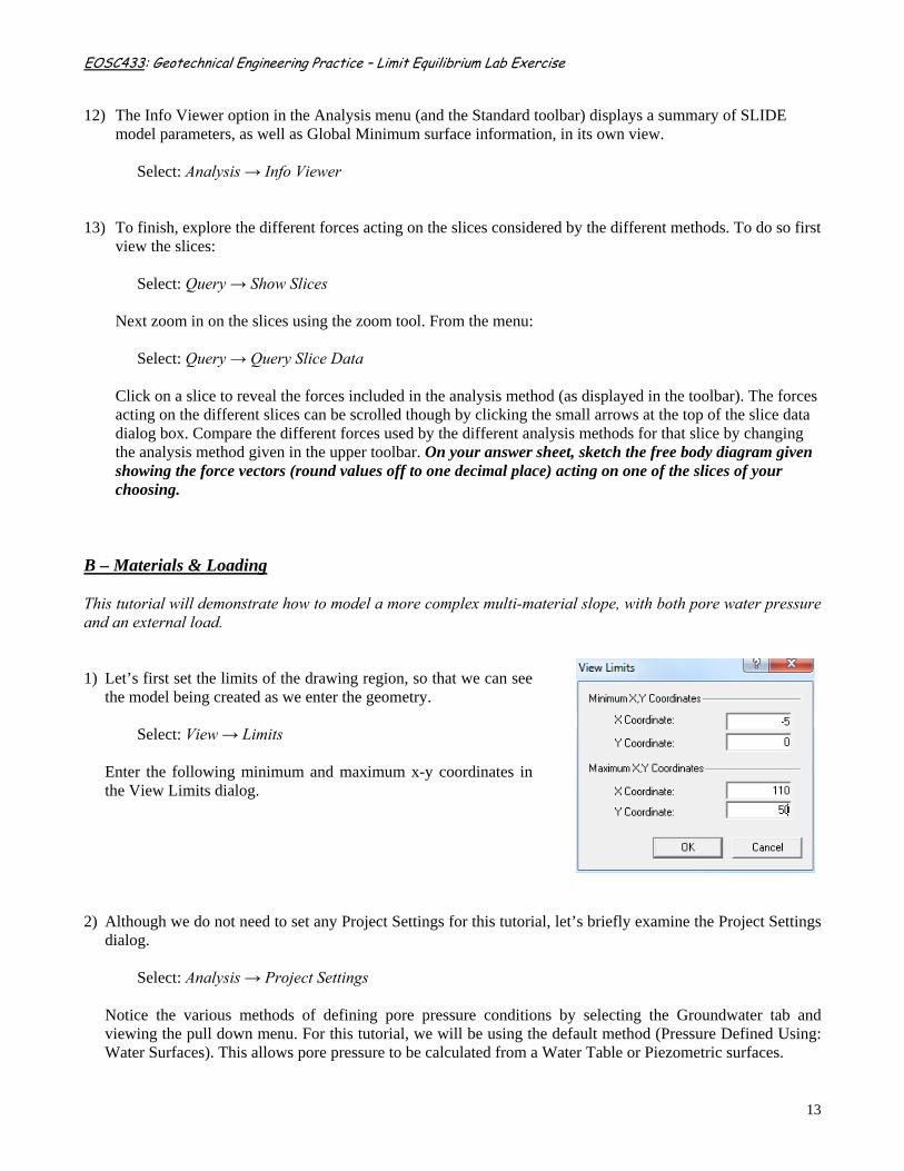
B – Materials & Loading This tutorial will demonstrate how to model a more complex multi-material slope, with both pore water pressure and an external load. 1) Let’s first set the limits of the drawing region, so that we can see
the model being created as we enter the geometry.
Select: View → Limits
Enter the following minimum and maximum x-y coordinates in the View Limits dialog.
2) Although we do not need to set any Project Settings for this tutorial, let’s briefly examine the Project Settings dialog.
Select: Analysis → Project Settings
Notice the various methods of defining pore pressure conditions by selecting the Groundwater tab and viewing the pull down menu. For this tutorial, we will be using the default method (Pressure Defined Using: Water Surfaces). This allows pore pressure to be calculated from a Water Table or Piezometric surfaces.
EOSC433: Geotechnical Engineering Practice – Limit Equilibrium Lab Exercise
14
3) To add the External Boundary, select Add External Boundary from the Boundaries menu or the Boundaries toolbar. Select: Boundaries → Add External Boundary Enter the coordinates given to the right in the prompt line at the bottom right of the screen. Note that entering c after the last vertex has been entered, automatically connects the first and last vertices (closes the boundary), and exits the Add External Boundary option.
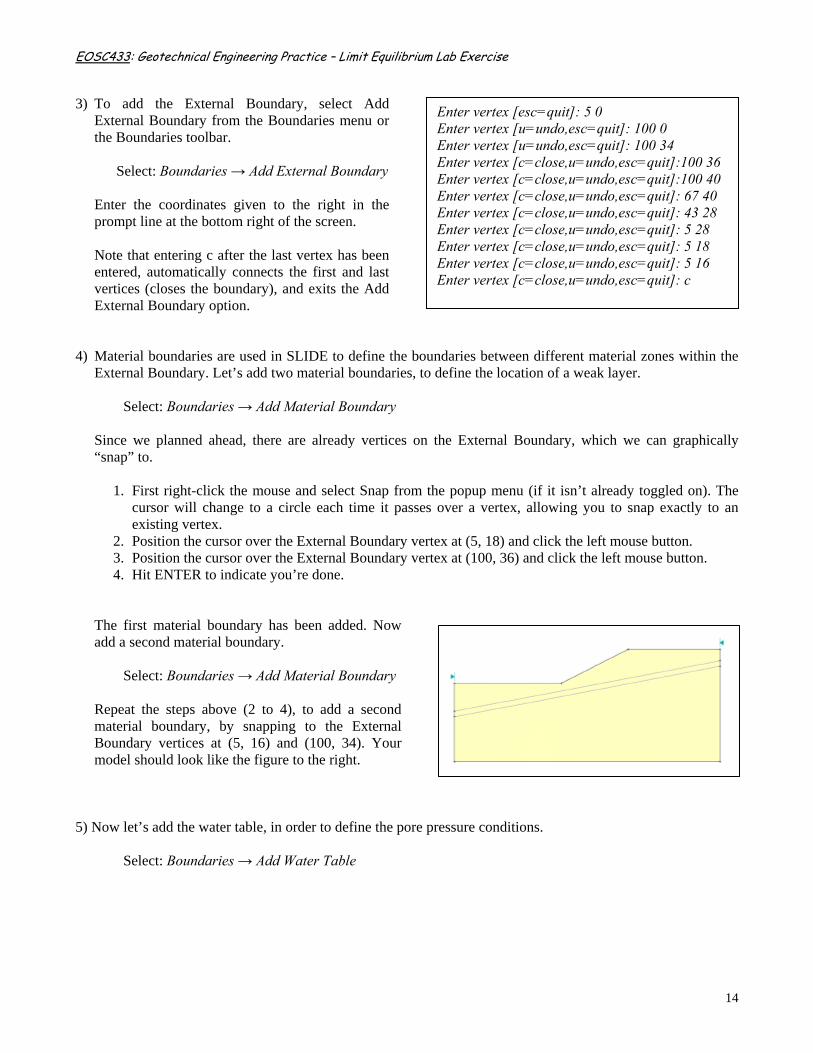
4) Material boundaries are used in SLIDE to define the boundaries between different material zones within the External Boundary. Let’s add two material boundaries, to define the location of a weak layer.
Select: Boundaries → Add Material Boundary
Since we planned ahead, there are already vertices on the External Boundary, which we can graphically “snap” to.
1. First right-click the mouse and select Snap from the popup menu (if it isn’t already toggled on). The cursor will change to a circle each time it passes over a vertex, allowing you to snap exactly to an existing vertex.
2. Position the cursor over the External Boundary vertex at (5, 18) and click the left mouse button. 3. Position the cursor over the External Boundary vertex at (100, 36) and click the left mouse button. 4. Hit ENTER to indicate you’re done.
The first material boundary has been added. Now add a second material boundary.
Select: Boundaries → Add Material Boundary Repeat the steps above (2 to 4), to add a second material boundary, by snapping to the External Boundary vertices at (5, 16) and (100, 34). Your model should look like the figure to the right.
5) Now let’s add the water table, in order to define the pore pressure conditions.
Select: Boundaries → Add Water Table
Enter vertex [esc=quit]: 5 0 Enter vertex [u=undo,esc=quit]: 100 0 Enter vertex [u=undo,esc=quit]: 100 34 Enter vertex [c=close,u=undo,esc=quit]:100 36 Enter vertex [c=close,u=undo,esc=quit]:100 40 Enter vertex [c=close,u=undo,esc=quit]: 67 40 Enter vertex [c=close,u=undo,esc=quit]: 43 28 Enter vertex [c=close,u=undo,esc=quit]: 5 28 Enter vertex [c=close,u=undo,esc=quit]: 5 18 Enter vertex [c=close,u=undo,esc=quit]: 5 16 Enter vertex [c=close,u=undo,esc=quit]: c
EOSC433: Geotechnical Engineering Practice – Limit Equilibrium Lab Exercise
15
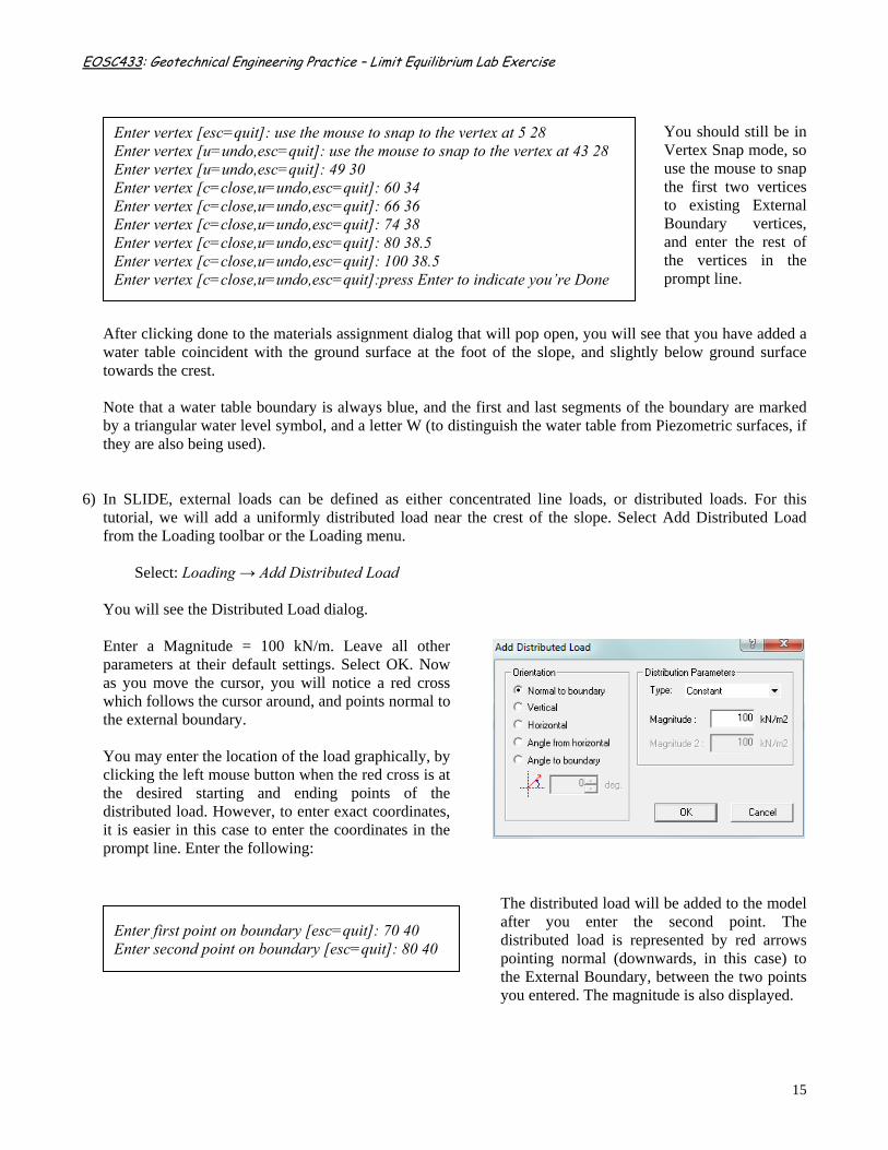
You should still be in Vertex Snap mode, so use the mouse to snap the first two vertices to existing External Boundary vertices, and enter the rest of the vertices in the prompt line.
After clicking done to the materials assignment dialog that will pop open, you will see that you have added a water table coincident with the ground surface at the foot of the slope, and slightly below ground surface towards the crest. Note that a water table boundary is always blue, and the first and last segments of the boundary are marked by a triangular water level symbol, and a letter W (to distinguish the water table from Piezometric surfaces, if they are also being used).
6) In SLIDE, external loads can be defined as either concentrated line loads, or distributed loads. For this tutorial, we will add a uniformly distributed load near the crest of the slope. Select Add Distributed Load from the Loading toolbar or the Loading menu.
Select: Loading → Add Distributed Load
You will see the Distributed Load dialog. Enter a Magnitude = 100 kN/m. Leave all other parameters at their default settings. Select OK. Now as you move the cursor, you will notice a red cross which follows the cursor around, and points normal to the external boundary. You may enter the location of the load graphically, by clicking the left mouse button when the red cross is at the desired starting and ending points of the distributed load. However, to enter exact coordinates, it is easier in this case to enter the coordinates in the prompt line. Enter the following:
The distributed load will be added to the model after you enter the second point. The distributed load is represented by red arrows pointing normal (downwards, in this case) to the External Boundary, between the two points you entered. The magnitude is also displayed.
Enter vertex [esc=quit]: use the mouse to snap to the vertex at 5 28 Enter vertex [u=undo,esc=quit]: use the mouse to snap to the vertex at 43 28 Enter vertex [u=undo,esc=quit]: 49 30 Enter vertex [c=close,u=undo,esc=quit]: 60 34 Enter vertex [c=close,u=undo,esc=quit]: 66 36 Enter vertex [c=close,u=undo,esc=quit]: 74 38 Enter vertex [c=close,u=undo,esc=quit]: 80 38.5 Enter vertex [c=close,u=undo,esc=quit]: 100 38.5 Enter vertex [c=close,u=undo,esc=quit]:press Enter to indicate you’re Done
Enter first point on boundary [esc=quit]: 70 40 Enter second point on boundary [esc=quit]: 80 40
EOSC433: Geotechnical Engineering Practice – Limit Equilibrium Lab Exercise
16
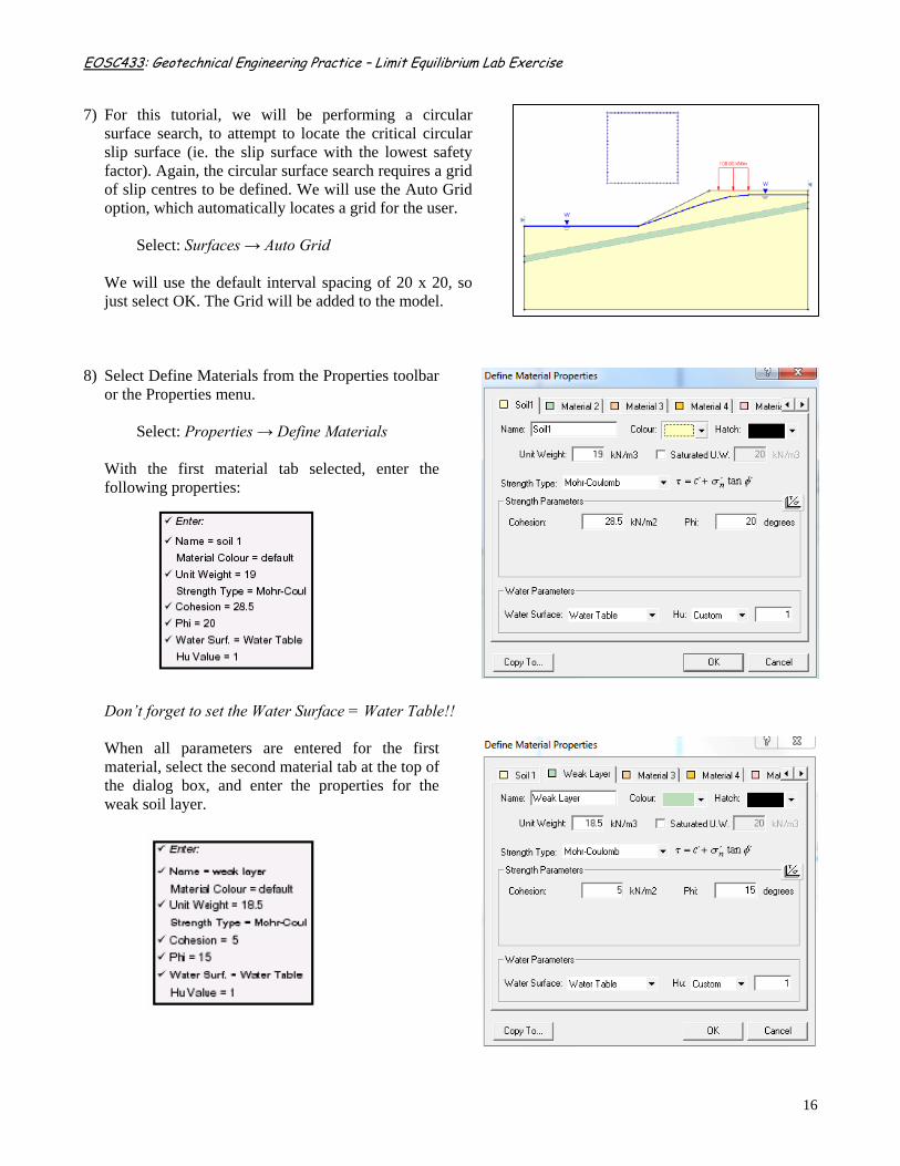
7) For this tutorial, we will be performing a circular surface search, to attempt to locate the critical circular slip surface (ie. the slip surface with the lowest safety factor). Again, the circular surface search requires a grid of slip centres to be defined. We will use the Auto Grid option, which automatically locates a grid for the user.
Select: Surfaces → Auto Grid
We will use the default interval spacing of 20 x 20, so just select OK. The Grid will be added to the model.
8) Select Define Materials from the Properties toolbar or the Properties menu.
Select: Properties → Define Materials
With the first material tab selected, enter the following properties:
Don’t forget to set the Water Surface = Water Table!! When all parameters are entered for the first material, select the second material tab at the top of the dialog box, and enter the properties for the weak soil layer.
EOSC433: Geotechnical Engineering Practice – Limit Equilibrium Lab Exercise
17
Note the following about the Water Parameters:
• You must specify the Water Surface = Water Table, in order to specify that the Water Table is used for pore pressure calculations, for a given soil.
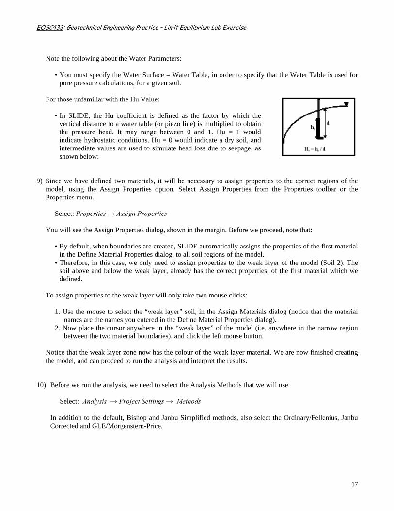
For those unfamiliar with the Hu Value:
• In SLIDE, the Hu coefficient is defined as the factor by which the vertical distance to a water table (or piezo line) is multiplied to obtain the pressure head. It may range between 0 and 1. Hu = 1 would indicate hydrostatic conditions. Hu = 0 would indicate a dry soil, and intermediate values are used to simulate head loss due to seepage, as shown below:
9) Since we have defined two materials, it will be necessary to assign properties to the correct regions of the model, using the Assign Properties option. Select Assign Properties from the Properties toolbar or the Properties menu.
Select: Properties → Assign Properties
You will see the Assign Properties dialog, shown in the margin. Before we proceed, note that:
• By default, when boundaries are created, SLIDE automatically assigns the properties of the first material in the Define Material Properties dialog, to all soil regions of the model.
• Therefore, in this case, we only need to assign properties to the weak layer of the model (Soil 2). The soil above and below the weak layer, already has the correct properties, of the first material which we defined.
To assign properties to the weak layer will only take two mouse clicks:
1. Use the mouse to select the “weak layer” soil, in the Assign Materials dialog (notice that the material names are the names you entered in the Define Material Properties dialog).
2. Now place the cursor anywhere in the “weak layer” of the model (i.e. anywhere in the narrow region between the two material boundaries), and click the left mouse button.
Notice that the weak layer zone now has the colour of the weak layer material. We are now finished creating the model, and can proceed to run the analysis and interpret the results.
10) Before we run the analysis, we need to select the Analysis Methods that we will use.
Select: Analysis → Project Settings → Methods
In addition to the default, Bishop and Janbu Simplified methods, also select the Ordinary/Fellenius, Janbu Corrected and GLE/Morgenstern-Price.
EOSC433: Geotechnical Engineering Practice – Limit Equilibrium Lab Exercise
18
11) Before you analyze your model, save it as a file called ml_circ.sli. (SLIDE model files have a .SLI filename extension). DON’T FORGET TO SAVE, as you will be using the same model later on.
Select: File → Save
Use the Save As dialog to save the file. You are now ready to run the analysis.
Select: Analysis → Compute
The SLIDE COMPUTE engine will proceed in running the analysis. When completed, you are ready to view the results in INTERPRET.
12) To view the results of the analysis:
Select: Analysis → Interpret This will start the SLIDE INTERPRET program. Experiment with the different INTERPRET options. For each of the different analysis methods employed, record the respective Factor of Safety value on your exercise answer sheet!
13) As you can see, the Global Minimum slip circle passes through the weak layer and is partially underneath
the distributed load. As such, it appears that the weak layer and the external load clearly have an influence on the stability of this model. To test this, we will rerun the analysis without the external load.
Return to the SLIDE modeller window (showing your initial problem geometry) and delete the external load:
Select: Loading → Delete Load Then with the mouse, click on the load (the red lines representing the applied load should turn to dashed lines), and then hit the enter key to indicate you are done. This will delete the load.
14) Now, Go to File > Save as. Save your modified file calling it ml_circ2.sli and re-compute the analysis.
Select: Analysis → Compute
The SLIDE COMPUTE engine will proceed in running the analysis. When completed, use INTERPRET to review the results. For each of the different analysis methods employed, record the respective Factor of Safety value on your exercise answer sheet! BONUS: Reopen your initial saved geometry ml_circ.sli, save it as ml_circ3.sli, and by testing different
loads, determine the maximum load that can be applied to the top of the slope without dropping the factor of safety below 1.0 (based on GLE/Morgenstern Price). This can be done by using the modify load option in the loading menu, and then repeating the analysis.
EOSC433: Geotechnical Engineering Practice – Limit Equilibrium Lab Exercise
19
C – Non-Circular Surfaces This tutorial will use the same model as the previous tutorial (Part B: Materials & Loading), to demonstrate how an analysis can be performed using non-circular (piece-wise linear) slip surfaces. 1) Since we are using exactly the same model from the previous tutorial, we will not repeat the modeling
procedure, but simply read in the first saved file (file: ml_circ.sli). If you did not save this file or modified it and accidentally saved over it, then quickly re-enter the data
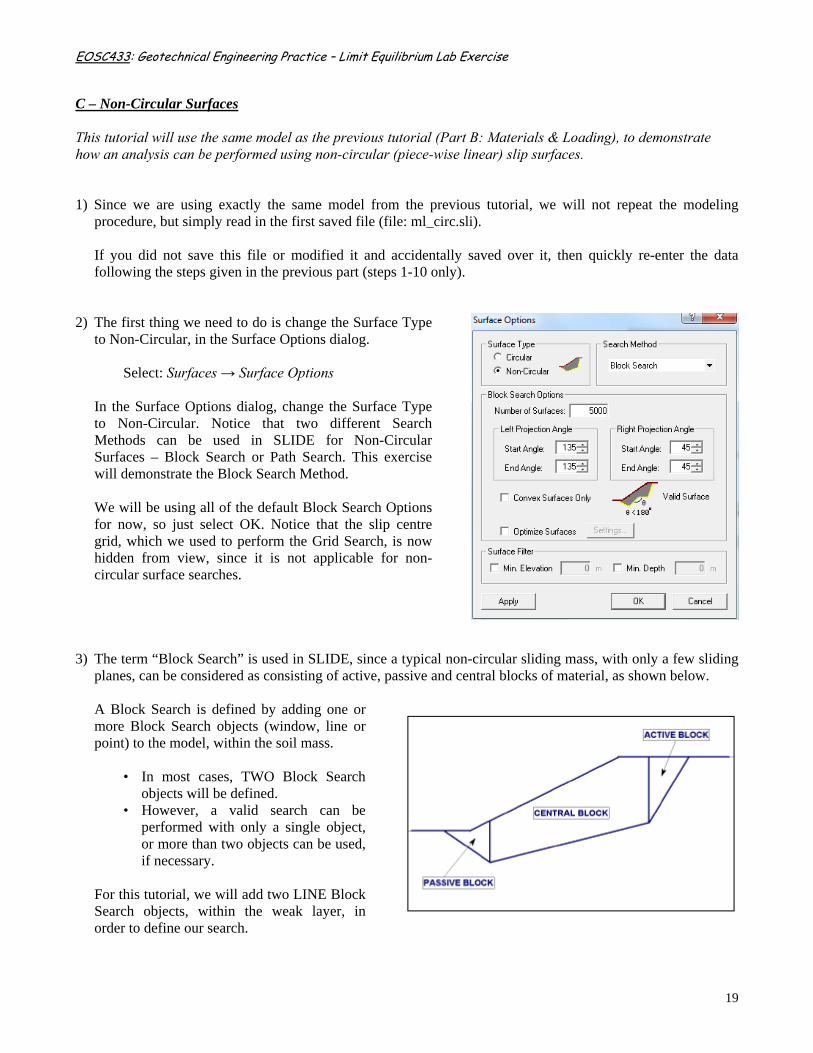
following the steps given in the previous part (steps 1-10 only). 2) The first thing we need to do is change the Surface Type
to Non-Circular, in the Surface Options dialog.
Select: Surfaces → Surface Options
In the Surface Options dialog, change the Surface Type to Non-Circular. Notice that two different Search Methods can be used in SLIDE for Non-Circular Surfaces – Block Search or Path Search. This exercise will demonstrate the Block Search Method. We will be using all of the default Block Search Options for now, so just select OK. Notice that the slip centre grid, which we used to perform the Grid Search, is now hidden from view, since it is not applicable for non-circular surface searches.
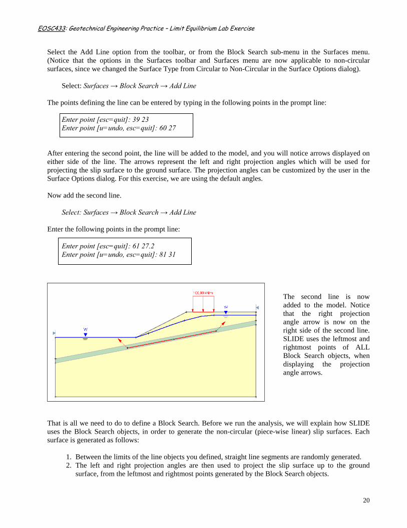
3) The term “Block Search” is used in SLIDE, since a typical non-circular sliding mass, with only a few sliding
planes, can be considered as consisting of active, passive and central blocks of material, as shown below.
A Block Search is defined by adding one or more Block Search objects (window, line or point) to the model, within the soil mass.
• In most cases, TWO Block Search objects will be defined.
• However, a valid search can be performed with only a single object, or more than two objects can be used, if necessary.
For this tutorial, we will add two LINE Block Search objects, within the weak layer, in order to define our search.
EOSC433: Geotechnical Engineering Practice – Limit Equilibrium Lab Exercise
20
Select the Add Line option from the toolbar, or from the Block Search sub-menu in the Surfaces menu. (Notice that the options in the Surfaces toolbar and Surfaces menu are now applicable to non-circular surfaces, since we changed the Surface Type from Circular to Non-Circular in the Surface Options dialog).
Select: Surfaces → Block Search → Add Line The points defining the line can be entered by typing in the following points in the prompt line:
Enter point [esc=quit]: 39 23 Enter point [u=undo, esc=quit]: 60 27
After entering the second point, the line will be added to the model, and you will notice arrows displayed on either side of the line. The arrows represent the left and right projection angles which will be used for projecting the slip surface to the ground surface. The projection angles can be customized by the user in the Surface Options dialog. For this exercise, we are using the default angles. Now add the second line.
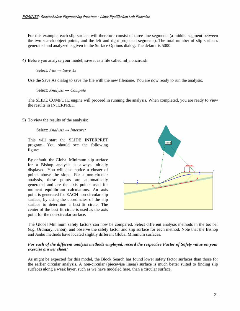
Select: Surfaces → Block Search → Add Line Enter the following points in the prompt line:
Enter point [esc=quit]: 61 27.2 Enter point [u=undo, esc=quit]: 81 31
The second line is now added to the model. Notice that the right projection angle arrow is now on the right side of the second line. SLIDE uses the leftmost and rightmost points of ALL Block Search objects, when displaying the projection angle arrows.
That is all we need to do to define a Block Search. Before we run the analysis, we will explain how SLIDE uses the Block Search objects, in order to generate the non-circular (piece-wise linear) slip surfaces. Each surface is generated as follows:
1. Between the limits of the line objects you defined, straight line segments are randomly generated. 2. The left and right projection angles are then used to project the slip surface up to the ground
surface, from the leftmost and rightmost points generated by the Block Search objects.
EOSC433: Geotechnical Engineering Practice – Limit Equilibrium Lab Exercise
21
For this example, each slip surface will therefore consist of three line segments (a middle segment between the two search object points, and the left and right projected segments). The total number of slip surfaces generated and analyzed is given in the Surface Options dialog. The default is 5000.
4) Before you analyze your model, save it as a file called ml_noncirc.sli.
Select: File → Save As Use the Save As dialog to save the file with the new filename. You are now ready to run the analysis.
Select: Analysis → Compute The SLIDE COMPUTE engine will proceed in running the analysis. When completed, you are ready to view the results in INTERPRET.
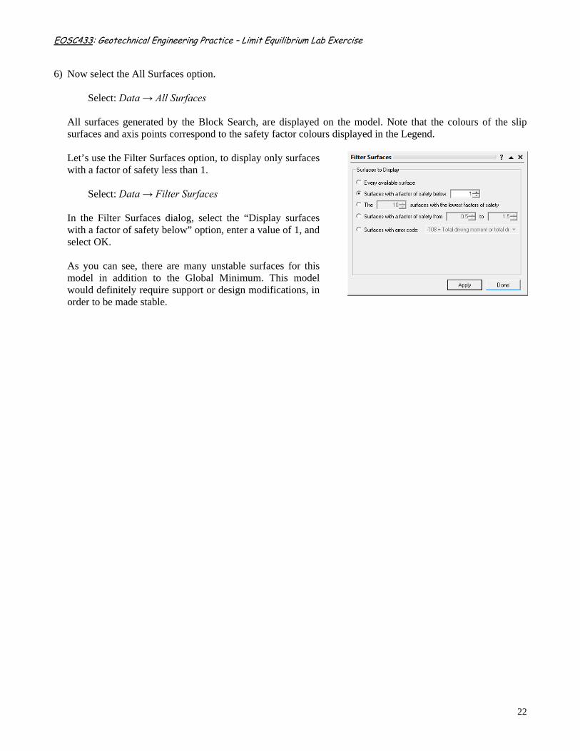
5) To view the results of the analysis:
Select: Analysis → Interpret This will start the SLIDE INTERPRET program. You should see the following figure: By default, the Global Minimum slip surface for a Bishop analysis is always initially displayed. You will also notice a cluster of points above the slope. For a non-circular analysis, these points are automatically generated and are the axis points used for moment equilibrium calculations. An axis point is generated for EACH non-circular slip surface, by using the coordinates of the slip surface to determine a best-fit circle. The center of the best-fit circle is used as the axis point for the non-circular surface. The Global Minimum safety factors can now be compared. Select different analysis methods in the toolbar (e.g. Ordinary, Janbu), and observe the safety factor and slip surface for each method. Note that the Bishop and Janbu methods have located slightly different Global Minimum surfaces. For each of the different analysis methods employed, record the respective Factor of Safety value on your exercise answer sheet! As might be expected for this model, the Block Search has found lower safety factor surfaces than those for the earlier circular analysis. A non-circular (piecewise linear) surface is much better suited to finding slip surfaces along a weak layer, such as we have modeled here, than a circular surface.
EOSC433: Geotechnical Engineering Practice – Limit Equilibrium Lab Exercise
22
6) Now select the All Surfaces option.
Select: Data → All Surfaces All surfaces generated by the Block Search, are displayed on the model. Note that the colours of the slip surfaces and axis points correspond to the safety factor colours displayed in the Legend. Let’s use the Filter Surfaces option, to display only surfaces with a factor of safety less than 1.
Select: Data → Filter Surfaces
In the Filter Surfaces dialog, select the “Display surfaces with a factor of safety below” option, enter a value of 1, and select OK.
As you can see, there are many unstable surfaces for this model in addition to the Global Minimum. This model would definitely require support or design modifications, in order to be made stable.


![The relationship between limit equilibrium slope stability methods[1].pdf](https://img.pdfslide.us/doc/110x75/577cdc141a28ab9e78a9d104/the-relationship-between-limit-equilibrium-slope-stability-methods1pdf.jpg)