LAB MATERIAL VARIABLE STARS PROJECT

VARIABLE STARS PROJECTLAB MATERIAL

VARIABLE STAR LIGHTCURVES

LAB 1

LAB 1: VARIABLE STAR LIGHTCURVES

▸ In this lab we will acquaint ourselves with variable star lightcurves and a lightcurve in data. We will use the data from the ROTSE-I prototype telescope that ran from 1997-2000 to study gamma-ray bursts. This data, however, was taken in a way that allows for straightforward identification and study of short period variable stars.

▸ In order to analyze astronomical data, one needs to be familiar with a computer system (‘operating system’ or ‘OS’), and an analysis program. We will rely on the Linux OS, and the IDL programming platform for analysis.

▸ Our ultimate goal will be to find variable stars in fields of data taken from ROTSE-I and to measure the variable period and amplitude for those that are regular. We will ultimately use the lightcurve shape and other information to classify those variables that we identify. The final deliverable for this lab will be a report, adhering to typical research standards, of the work accomplished.


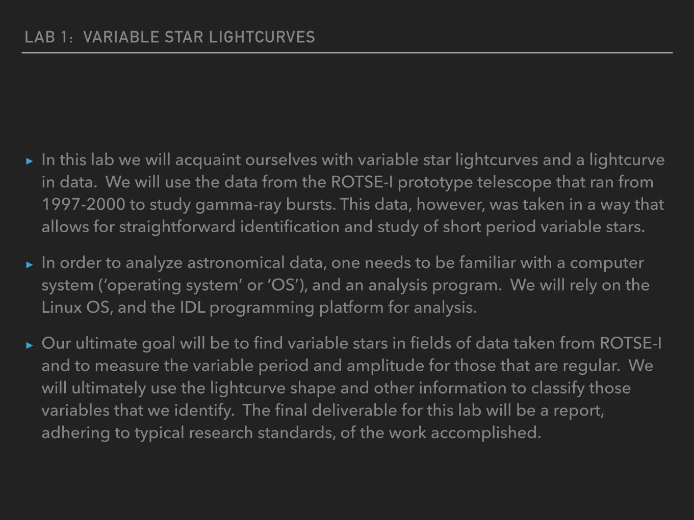
LINUX 101: BASIC COMMANDS▸ Login:

▸ Account: smurotse ▸ Password: ‘grb990123’

▸ On Linux command line: ▸ pwd: what is current directory or folder ▸ ls: list contents of current directory ▸ less: view or read a text file specified as

argument ▸ mkdir: make a new directory with name as

argument ▸ cd: change directory by specifying a ‘path

name’ as argument ▸ cp: copy one file to a new file with a

different name. Retains old file ▸ mv: rename a file. Original file is gone

▸ One really useful comment: ‘man’ for ‘manual pages’ for any Unix program

> pwd

> ls

> less .cshrc

> mkdir plots

> cd plots

> cp ../.cshrc cshrc_copy.txt

> mv cshrc_copy.txt copy.txt

R. Kehoe - VSP Labs


IDL 101: PROCEDURES AND FILES

▸ Log into analysis workstation in Rm 101 ▸ > ssh -Y [email protected]

▸ For this week, use ‘rotse1.physics.smu.edu’ though ▸ > password: ‘grb990123’

▸ Go to the directory where the data structures are: ▸ > cd phy3368/<your last name> ▸ > ls

▸ Read in our data, and examine the contents ▸ > IDL ▸ IDL> restore, ‘000409_xtetrans_1a_match.dat’

▸ This reads in the file and loads the data structure into memory for examination. Cameras 1a, 1b, 1c, 1d for each user.

5

mailto:[email protected]

R. Kehoe - VSP Labs


DATA STRUCTURES

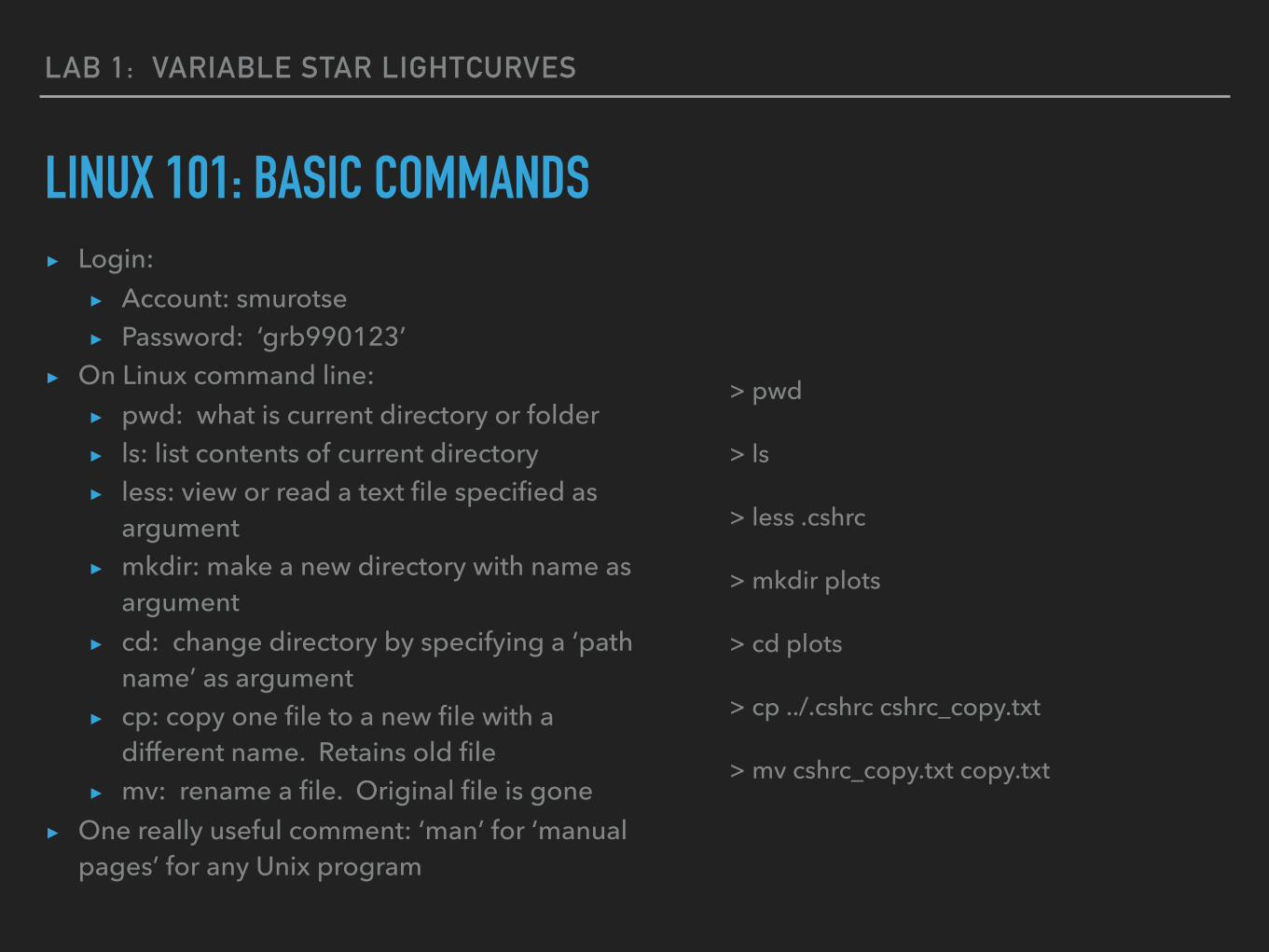
▸ To examine the overall ‘match structure’ ▸ IDL> help, match, /str

▸ Try this with the contents of the ‘match structure’ ▸ IDL> print, match.jd

▸ # Prints ‘Julián dates’ for observations ▸ IDL> print, match.m[*,1000], match.ra[1000], match.dec[1000]

▸ Print magnitudes, RA and Dec for all observations, ‘star’ 1000 ▸ IDL> print, match.m[120,1000:1100]

▸ Print magnitude for observation 120 for stars 1000 thru 1100

▸ Now, print the observation time for the first observation, and magnitude and coordinates of the first observation of the 1900th source in the match structure ▸ Then write down some attributes of your data you will want handy: ▸ # observations, # stars, starting and stopping time, field RA (RAC) and Dec (DECC)

6

R. Kehoe - VSP Labs


LIGHTCURVES

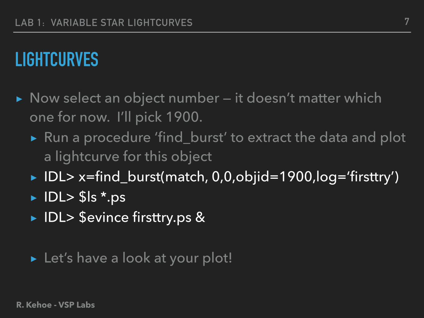
▸ Now select an object number — it doesn’t matter which one for now. I’ll pick 1900. ▸ Run a procedure ‘find_burst’ to extract the data and plot

a lightcurve for this object ▸ IDL> x=find_burst(match, 0,0,objid=1900,log=‘firsttry’) ▸ IDL> $ls *.ps ▸ IDL> $evince firsttry.ps &

▸ Let’s have a look at your plot!

7

R. Kehoe - VSP Labs


SUPPORTING MATERIAL

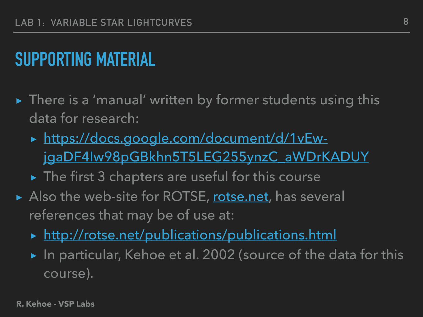
▸ There is a ‘manual’ written by former students using this data for research: ▸ https://docs.google.com/document/d/1vEw-

jgaDF4Iw98pGBkhn5T5LEG255ynzC_aWDrKADUY ▸ The first 3 chapters are useful for this course

▸ Also the web-site for ROTSE, rotse.net, has several references that may be of use at: ▸ http://rotse.net/publications/publications.html ▸ In particular, Kehoe et al. 2002 (source of the data for this

course).

8

https://docs.google.com/document/d/1vEw-jgaDF4Iw98pGBkhn5T5LEG255ynzC_aWDrKADUY

https://docs.google.com/document/d/1vEw-jgaDF4Iw98pGBkhn5T5LEG255ynzC_aWDrKADUY

http://rotse.net

http://rotse.net/publications/publications.html

R. Kehoe - VSP Labs


PROJECT REPORT OUTLINES▸ Research is most often communicated in papers published

in research journals, whether they be academic or trade journals. In this course, we will implement our report of the lab effort in a manner similar to the typical structure of these papers. As such, there are five typical sections:

▸ Introduction/Motivation: A section reviewing recent theoretical or experimental questions, with a summary of the state of experimental results.

▸ Detector/Apparatus: Summary of the key aspects of the experimental setup that yielded the data.

9

R. Kehoe - VSP Labs


PROJECT REPORT OUTLINES▸ Sections (cont.)

▸ Data Samples/Data Reduction: A section describing the nature of the data, how it was taken. It is also important to describe the earlier ‘data reduction’ pipeline that yielded the physically meaningful measurements in the match structures you will be using.

▸ Analysis/Results: Analysis steps, from selection, to background reduction, phasing and classification. Analysis results are provided.

▸ Conclusions: The most important final results are summarized here, with whatever evaluations can be made about shortcomings and potential future improvements or questions.

▸ There will also be an initial ‘Abstract’, and a final ‘References’ section.

10

FINDING VARIABLE STAR CANDIDATES

LAB 2

R. Kehoe - VSP Labs

LAB 2: FINDING VARIABLE STAR CANDIDATES

CCD PERFORMANCE: UNCORRELATED IMPACTS

▸ Dark current ▸ Production of free electrons per pixel vs. time - due to thermal

energy present ▸ Also results noise per pixel that increases as sqrt(t)

▸ Malfunctioning pixels/columns ▸ Hot pixels - generally produces wide variations in reported

charge independent of incident photons ▸ Bad columns ▸ can be a column that fails to be controlled properly ▸ Shows up as a column of very high charge

▸ Cosmic rays

12

R. Kehoe - VSP Labs


CCD PERFORMANCE: CORRELATED IMPACTS

▸ Several effects occur such that they scale with the # of photons incident on a pixel ▸ Pixel gain variations ▸ These are small changes in the # of electrons produced per #

incident photons ▸ Can be due to nonuniformities in Si, or in electronics variations

controlling pixels ▸ Gain variation across the field ▸ Vignetting: Aperture of telescope blocks out light from edges of

field more than center ▸ Shutter sticking and other impacts on amount of light onto

primary mirror

13

R. Kehoe - VSP Labs


DATA REDUCTION

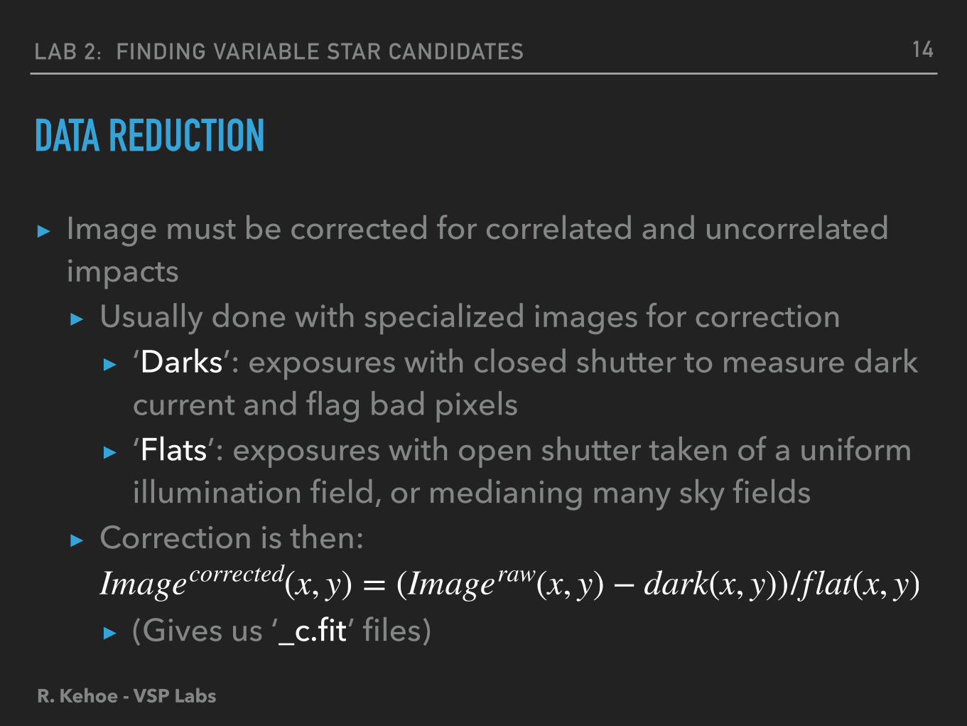
▸ Image must be corrected for correlated and uncorrelated impacts ▸ Usually done with specialized images for correction ▸ ‘Darks’: exposures with closed shutter to measure dark

current and flag bad pixels ▸ ‘Flats’: exposures with open shutter taken of a uniform

illumination field, or medianing many sky fields ▸ Correction is then:

▸ (Gives us ‘_c.fit’ files)Imagecorrected(x, y) = (Imageraw(x, y) − dark(x, y))/flat(x, y)

14

R. Kehoe - VSP Labs


SOURCE EXTRACTION

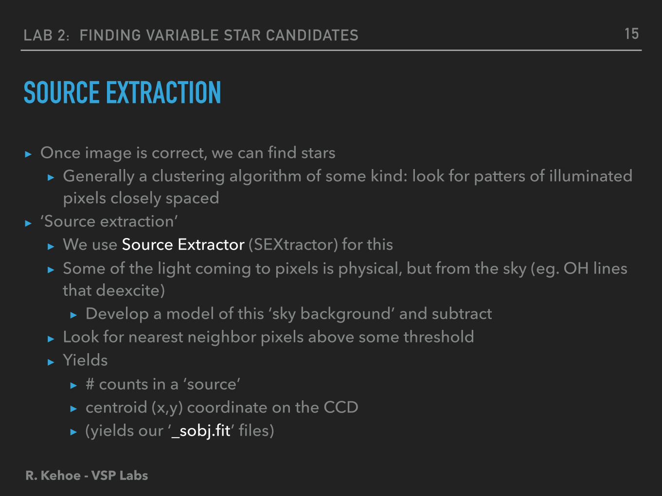
▸ Once image is correct, we can find stars ▸ Generally a clustering algorithm of some kind: look for patters of illuminated

pixels closely spaced ▸ ‘Source extraction’

▸ We use Source Extractor (SEXtractor) for this ▸ Some of the light coming to pixels is physical, but from the sky (eg. OH lines

that deexcite) ▸ Develop a model of this ‘sky background’ and subtract

▸ Look for nearest neighbor pixels above some threshold ▸ Yields

▸ # counts in a ‘source’ ▸ centroid (x,y) coordinate on the CCD ▸ (yields our ‘_sobj.fit’ files)

15

R. Kehoe - VSP Labs


ASTROMETRY▸ The array of sources arranged in rectangular (x,y) CCD coordinate grid

▸ This is a projection of the spherical astronomical coordinates (α,δ) onto a plane

▸ How to obtain astronomical coordinates ▸ Ie. Astrometry - measure position of sources ▸ Compare unique triangles of objects in (x,y) to unique triangles in a known

well-measured astronomical catalog ▸ Eg. USNO catalog ▸ Fit to 2D analytic functions transforming (x,y) to (α,δ)

▸ Termed ‘matching’ ▸ Once each calibrated object list is made, they can be easily matched to

each other ▸ since they are all in absolute common coordinate system (α,δ) ▸ This is how a ‘match structure’ is made (after next step of photometry)

16

R. Kehoe - VSP Labs


PHOTOMETRY▸ Each source has physical coordinates, but still # counts in terms of measure of

brightness ▸ We want brightness in some absolute measure of flux

▸ Eg. Magnitudes ▸ Now that we have the coordinate transformation

▸ We know what all of observed sources are in terms of USNO stars ▸ Compare measured # counts to the magnitudes for V or R band in USNO

▸ Fit the transformation relating the two ▸ Also determine, for field, magnitude at which efficiency to observe goes

to 50% — ‘limiting magnitude’ M_LIM ▸ Yields catalog of (mag, α, δ) from (#counts, x, y) ▸ While all stars are used in the comparison, including variable stars, the

average transformation is dominated by nonvariables and so we can still see them

▸ Astrometry and photometry yields ‘_cobj.fit’ from ‘_sobj.fit’

17

R. Kehoe - VSP Labs


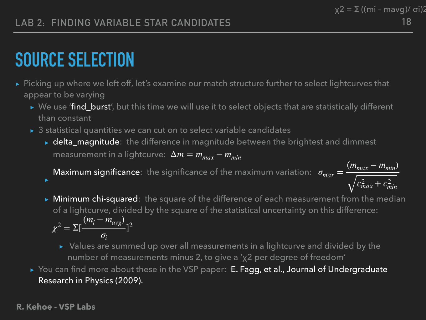
SOURCE SELECTION▸ Picking up where we left off, let’s examine our match structure further to select lightcurves that

appear to be varying ▸ We use ‘find_burst’, but this time we will use it to select objects that are statistically different

than constant ▸ 3 statistical quantities we can cut on to select variable candidates

▸ delta_magnitude: the difference in magnitude between the brightest and dimmest measurement in a lightcurve:

▸Maximum significance: the significance of the maximum variation:

▸ Minimum chi-squared: the square of the difference of each measurement from the median of a lightcurve, divided by the square of the statistical uncertainty on this difference:

▸ Values are summed up over all measurements in a lightcurve and divided by the number of measurements minus 2, to give a ‘χ2 per degree of freedom’

▸ You can find more about these in the VSP paper: E. Fagg, et al., Journal of Undergraduate Research in Physics (2009).

Δm = mmax − mmin

σmax =(mmax − mmin)

ϵ2max + ϵ2

min

χ2 = Σ[(mi − mavg)

σi]2

18χ2 = Σ ((mi – mavg)/ σi)2

R. Kehoe - VSP Labs


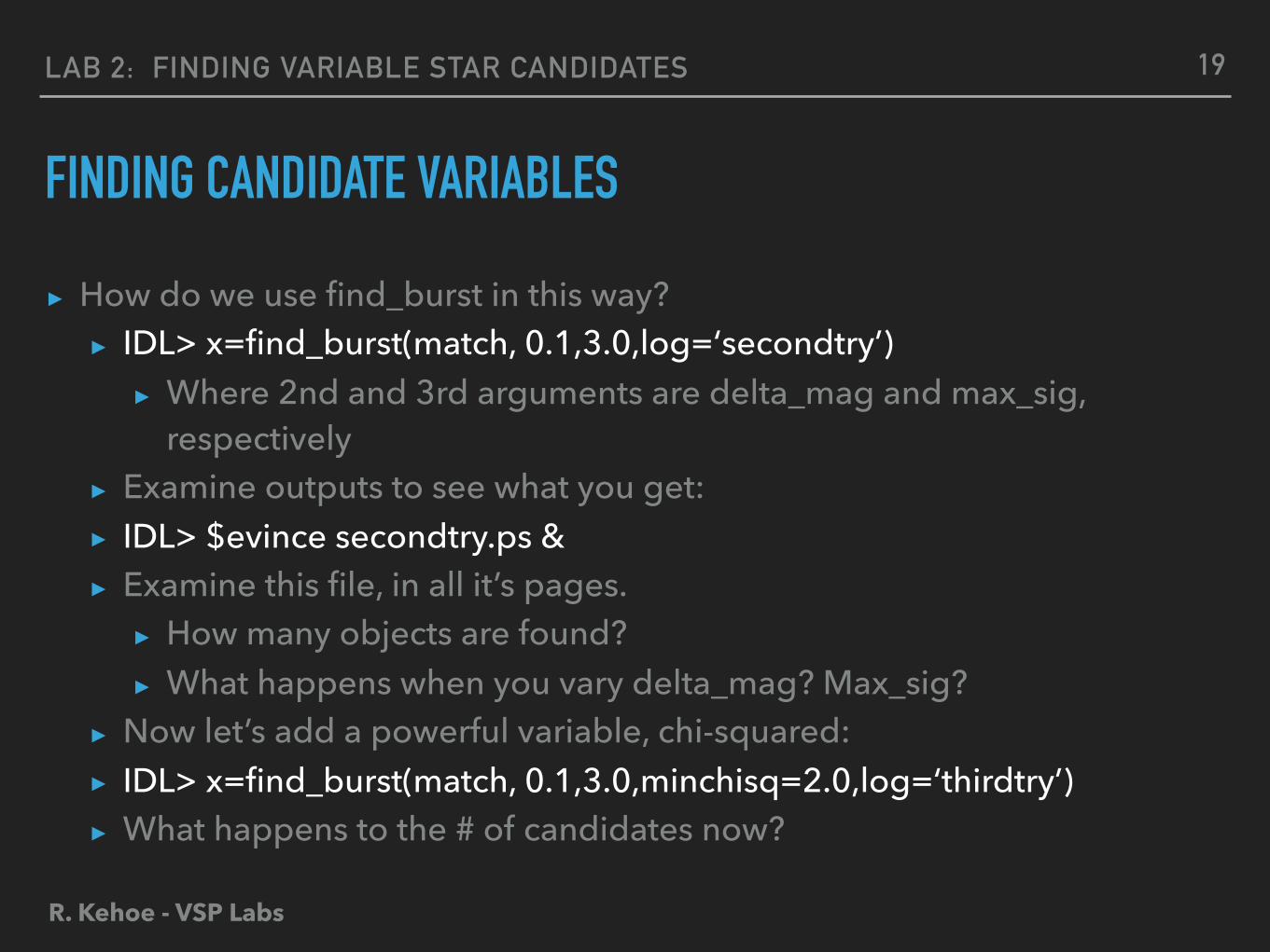
FINDING CANDIDATE VARIABLES

▸ How do we use find_burst in this way? ▸ IDL> x=find_burst(match, 0.1,3.0,log=‘secondtry’)

▸ Where 2nd and 3rd arguments are delta_mag and max_sig, respectively

▸ Examine outputs to see what you get: ▸ IDL> $evince secondtry.ps & ▸ Examine this file, in all it’s pages.

▸ How many objects are found? ▸ What happens when you vary delta_mag? Max_sig?

▸ Now let’s add a powerful variable, chi-squared: ▸ IDL> x=find_burst(match, 0.1,3.0,minchisq=2.0,log=‘thirdtry’) ▸ What happens to the # of candidates now?

19

R. Kehoe - VSP Labs


FINDING CANDIDATE VARIABLES

▸ Now, look at the individual lightcurves for all pages in your .ps files ▸ Can you pick out lightcurves that are physical, and those that

may be unphysical? ▸ Why are there lightcurves that are not physical? ▸ What is happening there?

▸ What physics could produce the physical lightcurves? ▸ You will notice a lot of ‘background’ from apparent variations that

have nothing to do with variables ▸ How do we handle these? ▸ We will revisit this next time.

20

R. Kehoe - VSP Labs


PROJECT REPORT: INTRODUCTION AND MOTIVATION

▸ In conducting research, it is important to establish the scientific questions that are more important to study. In presenting scientific research, we need to provide a review of these questions and description of how they related to each other, and the project at hand. These questions might be theoretical, or experimental/observational. In many cases, both are relevant. In this section of your report, you will:

▸ Conduct a literature search on a topic relevant to your research. For instance, the ‘period evolution of close eclipsing systems’

▸ Describe concisely the theoretical problems or questions that are recently in the literature, eg. What are theoretical predictions of time evolution of period?

▸ Also describe the current experimental or observational state of work in this area, eg. What sensitivities or surveys have been pursued to find such time evolution?

21

R. Kehoe - VSP Labs


PROJECT REPORT: INTRODUCTION AND MOTIVATION (CONT.)▸ Your 1st section will answer the above questions along the following lines:

▸ 2 or more pages ▸ Double spaced, 1” margins ▸ Not including Abstract, figures or tables, or references

▸ It will include at least one paragraph each covering the three main areas: ▸ What is the overall topic and why interesting generally ▸ What are the theoretical issues with this topic? ▸ What is the observational status of this research area?

▸ Plus a References Cited section at the end. Please aim to include at least 5 references from the literature (not including textbooks) in this draft. ▸ Suggested places to look for articles on-line: arxiv.org or adsabs.harvard.edu

▸ Put in some keywords to each and examine the search results

▸ This will be the first section of your final report, and this draft is due at mid-term as given on the syllabus.

22

http://arxiv.org

http://adsabs.harvard.edu

REDUCING BACKGROUNDS

LAB 3

R. Kehoe - VSP Labs

LAB 3: REDUCING BACKGROUNDS

TELESCOPE OPERATIONS

▸ Telescopes operated according to a scheme which is organized by target ▸ For ROTSE-I orphans data: Gamma-ray bursts (GRBs) ▸ In most cases, specific targets specified before observing ▸ Eg. Specific galaxies to measure in the Dark Energy

Survey

▸ Not all observations scheduled the same priority ▸ Variable stars may be scheduled lower priority than GRBs ▸ Affects when observations occur, and their frequency

24

R. Kehoe - VSP Labs


TELESCOPE OPERATIONS (CONT.)

▸ Seasonal and monthly cycles ▸ Targets rise and set at different times depending on season ▸ Moon up during observing some fraction of each month

▸ Moon injects more photons into sky during observations, ▸ Varies with phase ▸ particularly large when near full moon

▸ Sources observed lower in elevation (angle w/respect to horizon) ▸ Pass thru more air (more ‘airmass’)

▸ Scheduling ▸ Generally try to maximize ability to observe targets

▸ Favor low airmass, low moon, away from twilight ▸ Constrains when a particular field is best: constraints observing times

25

R. Kehoe - VSP Labs


SYSTEMATIC OBSERVING CHARACTERISTICS - PHOTOMETRY

▸ Weather presents differently at different times ▸ Eg. Opaque clouds, transparent clouds ▸ Sometimes limits time to observe: eg. rain, high winds

▸ Impacts on resolution ▸ Telescope optics must be focused, and often times this can vary over time

▸ Temperature shifts over night or longer can change where the focal plane lands relative to the detector, ie. Poor ‘focus’

▸ Atmospheric turbulence causes more smeared out stars, ‘seeing’ ▸ Even when observations can be made, these affects impact the measurement

▸ Transparent clouds in a portion of a field block out some light from sources there

▸ Vignetting variations per exposure similar impact locally light observed from a subset of sources

26

R. Kehoe - VSP Labs


TELESCOPE PERFORMANCE- ASTROMETRY

▸ Pointing ▸ Telescope has a conversion between hardware coordinates (on the

mechanical wheels on both axes) corresponding to RA and Dec ▸ Always some (small) error in reaching precise coordinates ▸ In some cases can be significant ▸ Sources at edges of field not observed, or observed anew

▸ Tracking ▸ Telescope must adjust pointing in real-time as Earth rotates ▸ Unevenness in wheels, or wear, can result in uneven tracking ▸ ‘Dumbells’ or elongated source shapes ▸ Might lead to problems in source extraction

27

R. Kehoe - VSP Labs


TELESCOPE PERFORMANCE- PHOTOMETRY

▸ Saturation ▸ The potential well of each pixel has finite height to its sides

▸ Can only hold so many electrons before some ‘spill out’ — saturation ▸ Electrons spill out in vertical, ‘y’, direction where potential barriers less (readout

direction) ▸ Hot pixels ▸ Coherent noise in CCD readout

▸ When the dark current of adjacent/nearby rows is correlated ▸ Cannot adequately subtract during data reduction, since dark current is different

each exposure ▸ Blending

▸ Two nearby objects are extracted as one object ▸ Or their division into two objects changes each exposure as exposure conditions

change ▸ Also can impact astrometry

28

R. Kehoe - VSP Labs


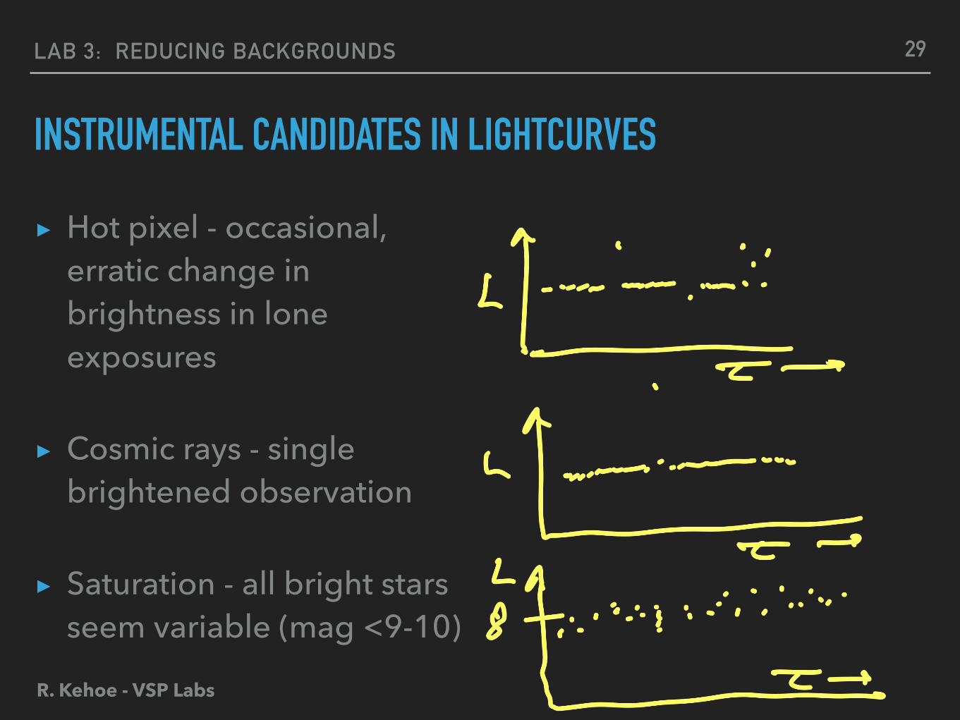
INSTRUMENTAL CANDIDATES IN LIGHTCURVES

▸ Hot pixel - occasional, erratic change in brightness in lone exposures

▸ Cosmic rays - single brightened observation

▸ Saturation - all bright stars seem variable (mag <9-10)

29

R. Kehoe - VSP Labs


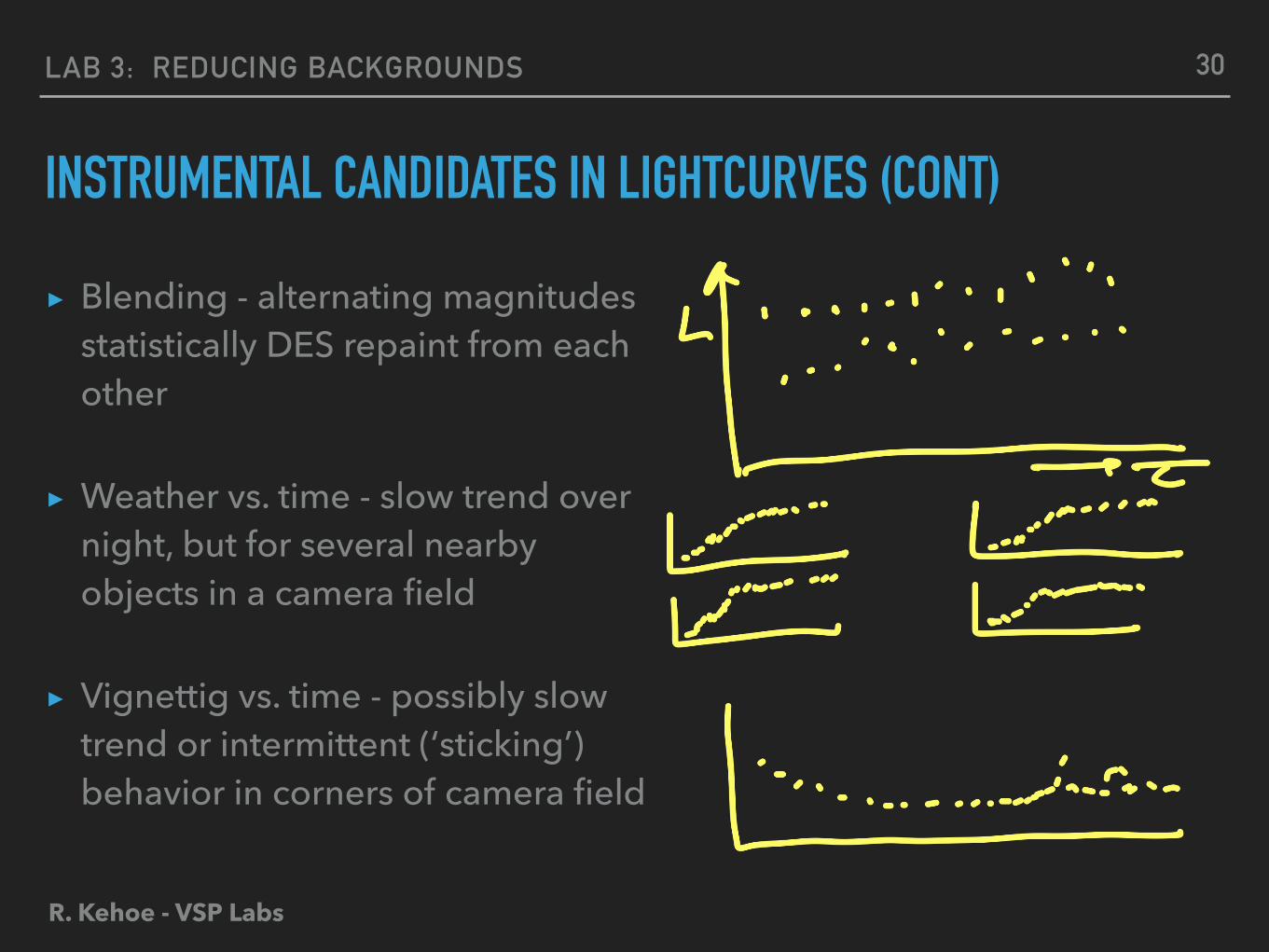
INSTRUMENTAL CANDIDATES IN LIGHTCURVES (CONT)

▸ Blending - alternating magnitudes statistically DES repaint from each other

▸ Weather vs. time - slow trend over night, but for several nearby objects in a camera field

▸ Vignettig vs. time - possibly slow trend or intermittent (‘sticking’) behavior in corners of camera field

30

R. Kehoe - VSP Labs


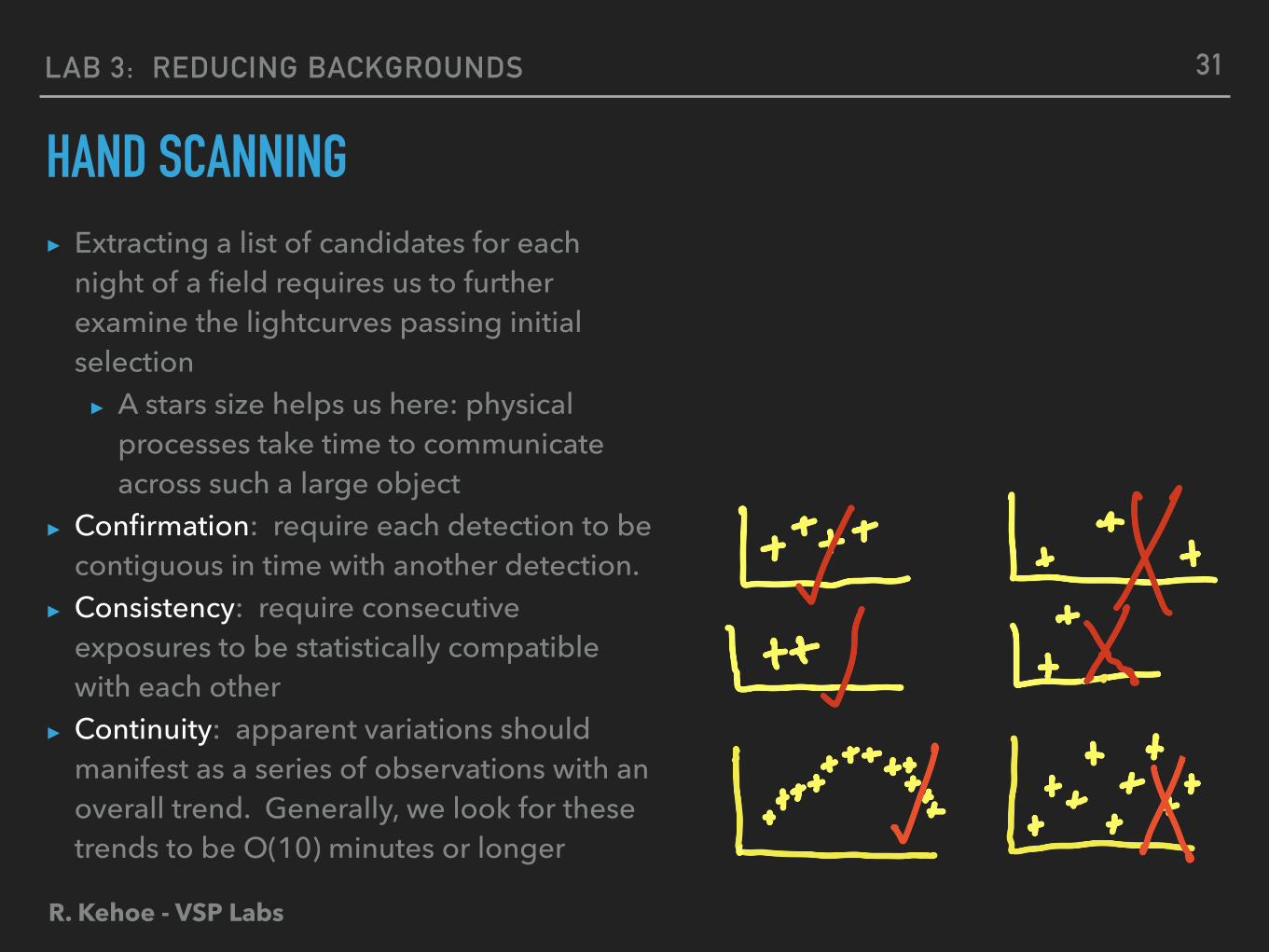
HAND SCANNING▸ Extracting a list of candidates for each

night of a field requires us to further examine the lightcurves passing initial selection ▸ A stars size helps us here: physical

processes take time to communicate across such a large object

▸ Confirmation: require each detection to be contiguous in time with another detection.

▸ Consistency: require consecutive exposures to be statistically compatible with each other

▸ Continuity: apparent variations should manifest as a series of observations with an overall trend. Generally, we look for these trends to be O(10) minutes or longer

31

R. Kehoe - VSP Labs


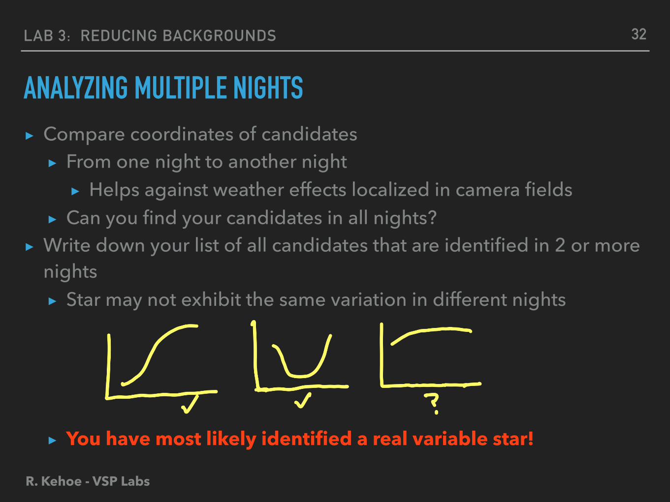
ANALYZING MULTIPLE NIGHTS▸ Compare coordinates of candidates ▸ From one night to another night ▸ Helps against weather effects localized in camera fields

▸ Can you find your candidates in all nights? ▸ Write down your list of all candidates that are identified in 2 or more

nights ▸ Star may not exhibit the same variation in different nights

▸ You have most likely identified a real variable star!

32

R. Kehoe - VSP Labs


FIRST PASS: PERIOD AND CLASSIFICATION

▸ For some variables ▸ A complete cycle, or nearly complete cycle visible in data you have ▸ Generally need maximum, and two minima in case it is an

eclipsing system ▸ Can you piece together a complete lightcurve?

▸ What is period? ▸ What is your guess as to classification?

33

PHASING LIGHTCURVES

LAB 4

R. Kehoe - VSP Labs

LAB 4: PHASING LIGHTCURVES

PROJECT REPORT: APPARATUS AND DATA

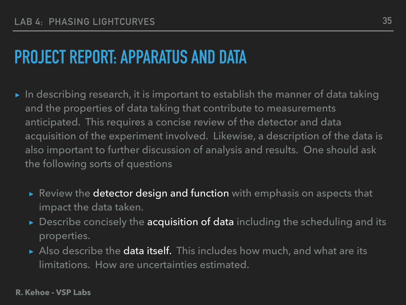
▸ In describing research, it is important to establish the manner of data taking and the properties of data taking that contribute to measurements anticipated. This requires a concise review of the detector and data acquisition of the experiment involved. Likewise, a description of the data is also important to further discussion of analysis and results. One should ask the following sorts of questions

▸ Review the detector design and function with emphasis on aspects that impact the data taken.

▸ Describe concisely the acquisition of data including the scheduling and its properties.

▸ Also describe the data itself. This includes how much, and what are its limitations. How are uncertainties estimated.

35

R. Kehoe - VSP Labs


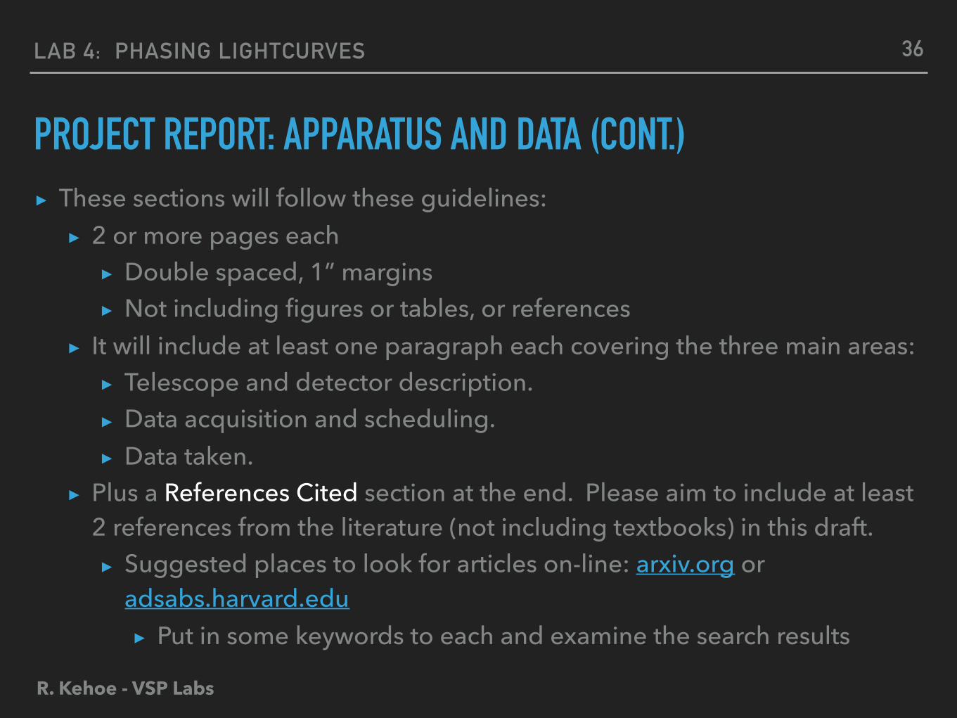
PROJECT REPORT: APPARATUS AND DATA (CONT.)▸ These sections will follow these guidelines:

▸ 2 or more pages each ▸ Double spaced, 1” margins ▸ Not including figures or tables, or references

▸ It will include at least one paragraph each covering the three main areas: ▸ Telescope and detector description. ▸ Data acquisition and scheduling. ▸ Data taken.

▸ Plus a References Cited section at the end. Please aim to include at least 2 references from the literature (not including textbooks) in this draft. ▸ Suggested places to look for articles on-line: arxiv.org or

adsabs.harvard.edu ▸ Put in some keywords to each and examine the search results

36

http://arxiv.org

http://adsabs.harvard.edu

R. Kehoe - VSP Labs


EXTRACTING LIGHTCURVE OBSERVATIONS▸ In order to reconstruct what the period of a regular variable is, we need to

employ a technique called ‘phasing’. In this approach, we apply a statistical algorithm that tests a range of hypotheses of period and amplitude until it identifies the best match.

▸ In order to phase a lightcurve, we require all of the time-domain data for a variable to be provided together. Assuming you have at least 2-3 variables with object IDs from 2 or more nights, we can begin.

▸ We first need to extract lightcurve data for each night. We need RA and Dec, the object ID for that night. In my case, I have a variable at 121036.89+461344.5 and it is obj ID 795 on April 9th: ▸ IDL> restore,’000409_xtetrans_1d_match.dat’ ▸ IDL> var=find_burst(match,0.0,0.0,objid=795,log=‘J1210+4613_409d’) ▸ This will produce a .ps file with just this objects lightcurve, and print the

measurements of the lightcurve to the screen.

37

J1145+5130: J1222+4838:

R. Kehoe - VSP Labs


EXTRACTING LIGHTCURVE OBSERVATIONS (CONT)▸ Now select and copy the printed measurements from the screen ▸ Open a text-based file with .dat extension: ▸ IDL> $vi J1210+4613.dat # Past table ▸ Commands in ‘vi;’: ‘i’ is insert, <Esc> gets out of insert mode, ‘dd’

deletes the current line, ‘ZZ’ escapes out of vi and saves the file. ▸ Repeat for subsequent nights ▸ IDL> restore,’000410_xtetrans_1d_match.dat’ ▸ ... ▸ IDL> restore,’000414_xtetrans_1d_match.dat’ ▸ ...

▸ Make sure to add each night after the previous, in time order. ▸ Remove all lines that have Magnitudes ~ 100, or errors ~99.

39

R. Kehoe - VSP Labs


PHASING▸ Phasing can be challenging due to the enormous range of periodic lightcurve

shapes. A widely separated eclipsing binary is mostly non-variable, and then has very sharp, deep minima. A contact binary system has a continuously varying lightcurve, and an RR Lyra tends to have a saw-tooth shaped lightcurve. ▸ We use a program, called ‘single_phase’ which employs a cubic spline fit

▸ Advantage: polynomial does not presuppose sinusoid all shape, and minimizes # fit parameters

▸ Disadvantage: loose information contained in Fourier analysis that is valuable for pulsating variables

▸ IDL> single_phase,’J1210+4613’,max_freq=30 ▸ Use file name without .dat extension. ▸ Produces output J1210+4613.txt file

▸ summarizes lightcurve and fit results

40

R. Kehoe - VSP Labs


PLOTTING PHASED LIGHTCURVE

▸ IDL> plot_datfile,’J1210+4613’,post=‘J1210+4613.ps’ ▸ If you identified your variable correctly, you should observe a

reasonable phased lightcurve plot ▸ IDL> $evince J1210+4613.ps &

▸ What are your period and amplitude? ▸ Does this lightcurve agree wth what you expected from the

nightly lightcurves? ▸ How many minima are there? Is that physical?

▸ Repeat for all of your confirmed variables.

41

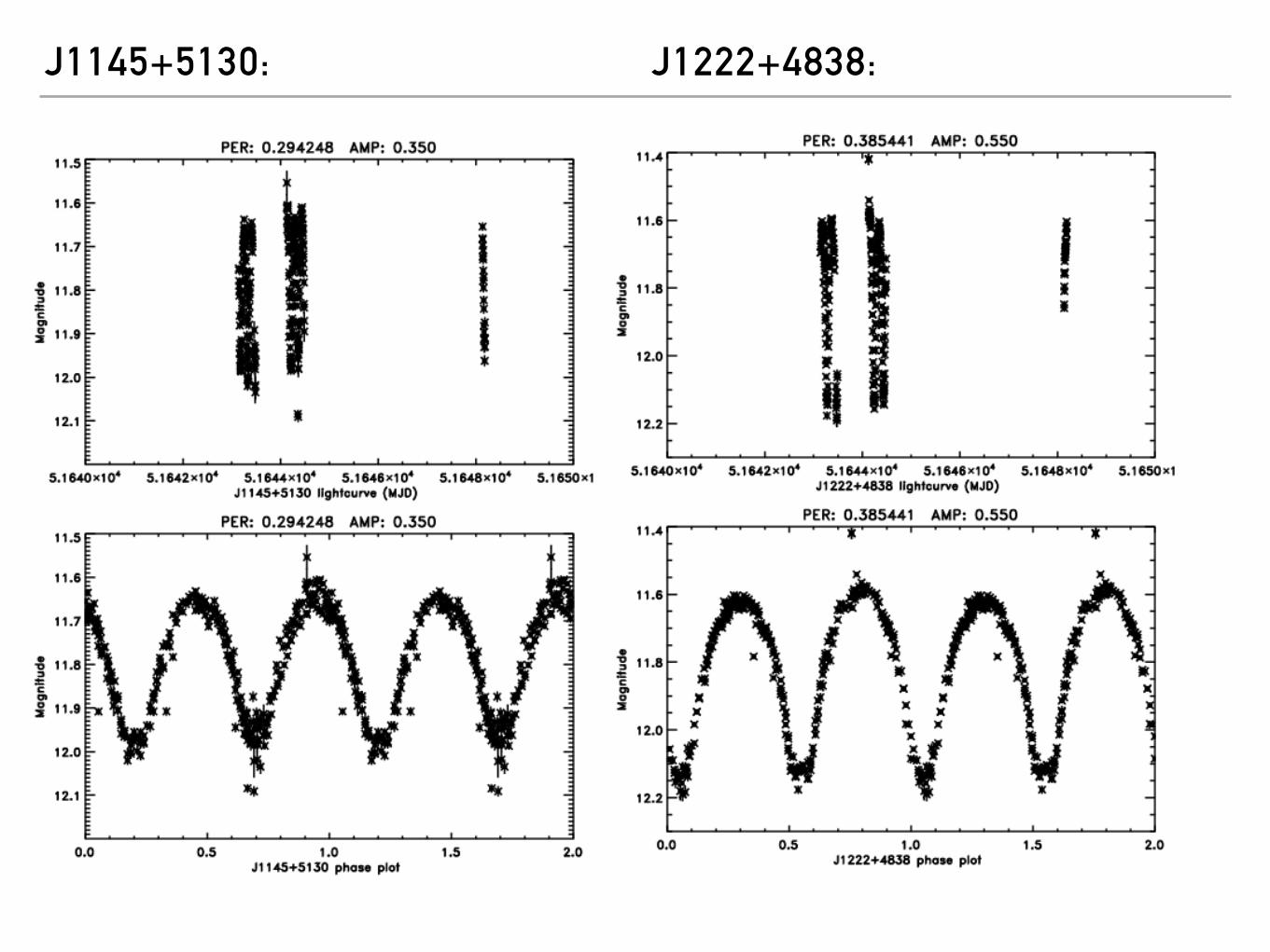
J1145+5130: J1222+4838:

R. Kehoe - VSP Labs


CHALLENGING CASES

▸ Sometimes there are relative photometry problems across nights ▸ Phasing things the dimmer night is indicating

a variation in brightness

▸ Erroneous data causes mismatch, and wrong period

43

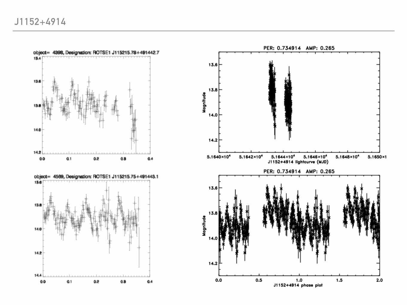
J1152+4914

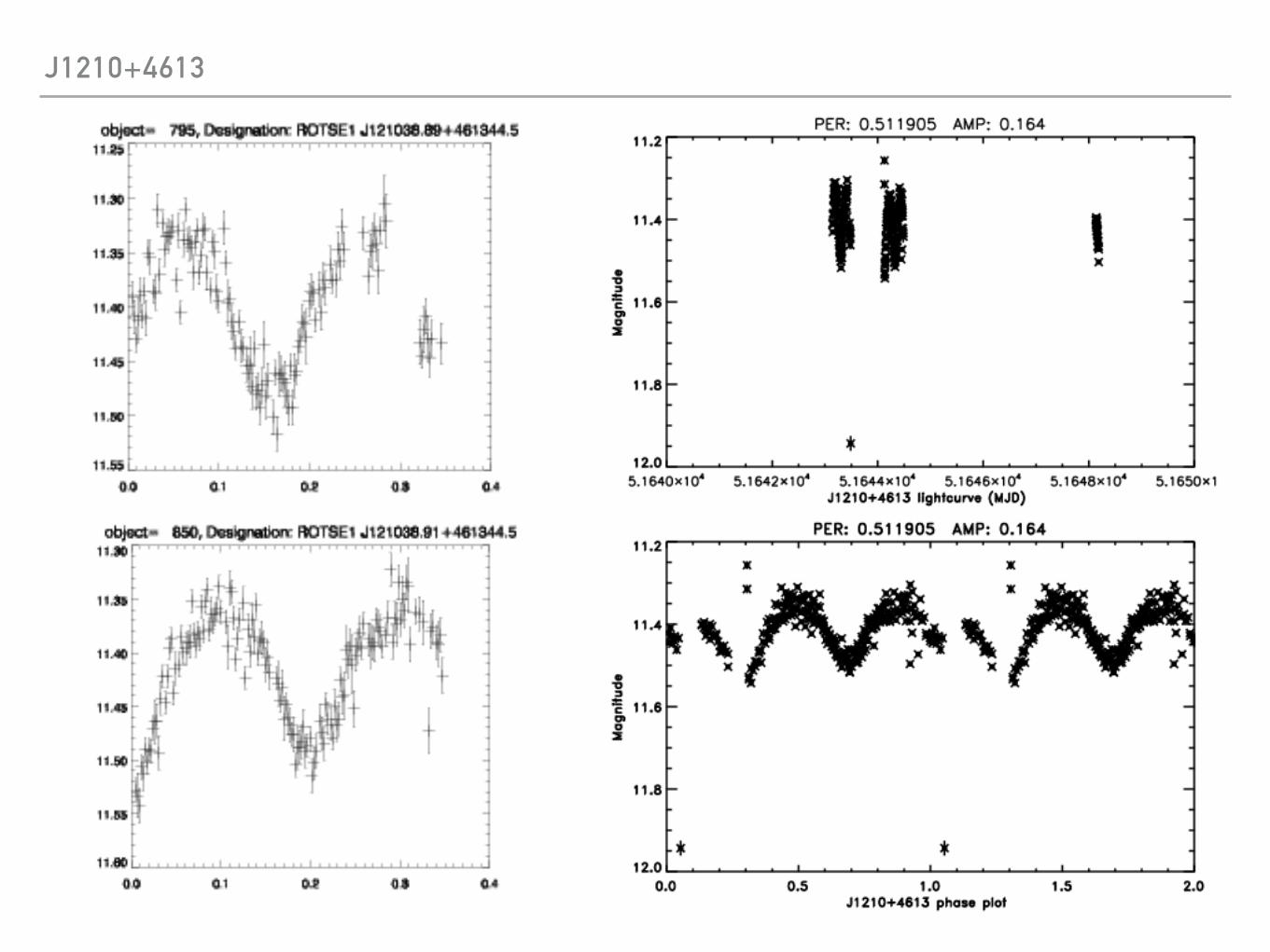
J1210+4613

CLASSIFICATIONLAB 5

R. Kehoe - VSP Labs

LAB 5: CLASSIFICATION

PROJECT REPORT: ANALYSIS AND RESULTS

▸ In describing research, it is important to provide the results of the analysis of the gathered data, and to explain the analysis applied to achieve those results. This requires the description of algorithmic steps in the analysis, as well as non-computation or by-hand steps. For instance, the statistical selection applied to nightly lightcurves should be e discussed, as well as the by-hand efforts to remove candidates with bad data or that are only observed on single nights. It also includes a discussion of the phasing analysis, with references. Additionally, the analysis goes beyond period, amplitude and classification, to involve the extraction of variable parameters , such as relative temperature, limits on orbital eccentricity, and orbit inclination, at least for subsets of the system types.

▸ Results should be primarily be contained in 3 tables: ▸ All variables confirmed in 2 or more nights that were not phased ▸ Variables that were phased, but the results are somehow in doubt. These will need

some discussion as to what the concern is, and what might be going on. ▸ All variables that were successfully phased

47

R. Kehoe - VSP Labs


PROJECT REPORT: ANALYSIS AND RESULTS (CONT.)▸ These sections may be together or appart but will follow these guidelines:

▸ 3 or more pages total ▸ Double spaced, 1” margins ▸ Not including figures or tables, or references

▸ Each will include at least one paragraph covering each of the three main areas: ▸ Analysis of statistical selection (find_burst), including visual inspection

and confirmation across two more nights ▸ Analysis of phasing, both the effective phasing we do by eye, and

especially the computational phasing ▸ Determination of physical properties of variable star system, including

statements on temperature, orientation and orbital properties ▸ Plus a References Cited section at the end. Please aim to include at least 2

references from the literature.

48

R. Kehoe - VSP Labs


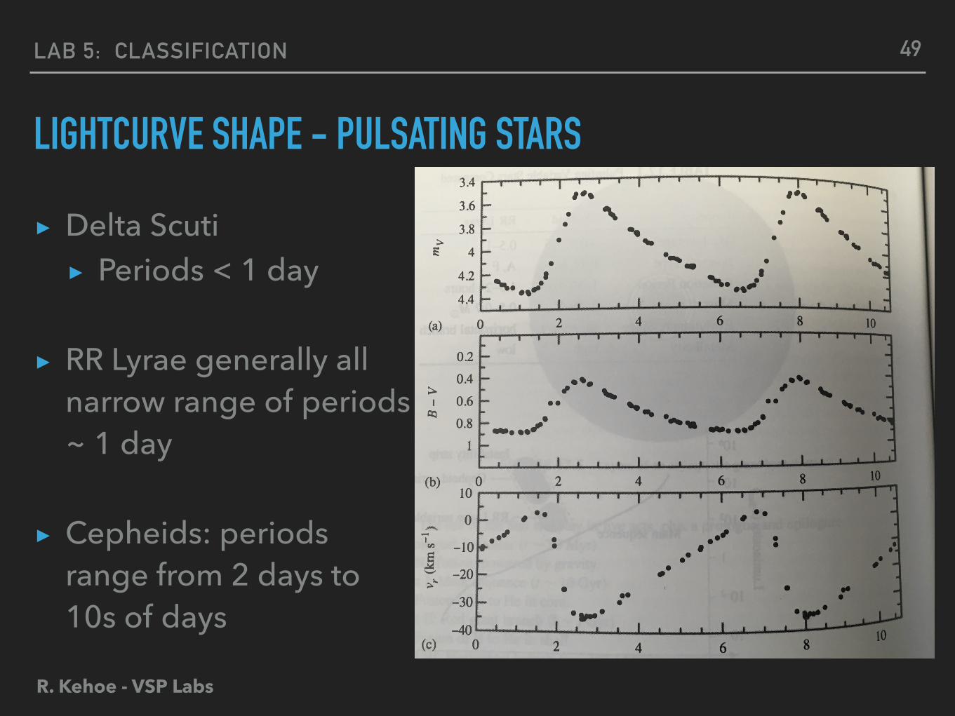
LIGHTCURVE SHAPE - PULSATING STARS

▸ Delta Scuti ▸ Periods < 1 day

▸ RR Lyrae generally all narrow range of periods ~ 1 day

▸ Cepheids: periods range from 2 days to 10s of days

49

R. Kehoe - VSP Labs


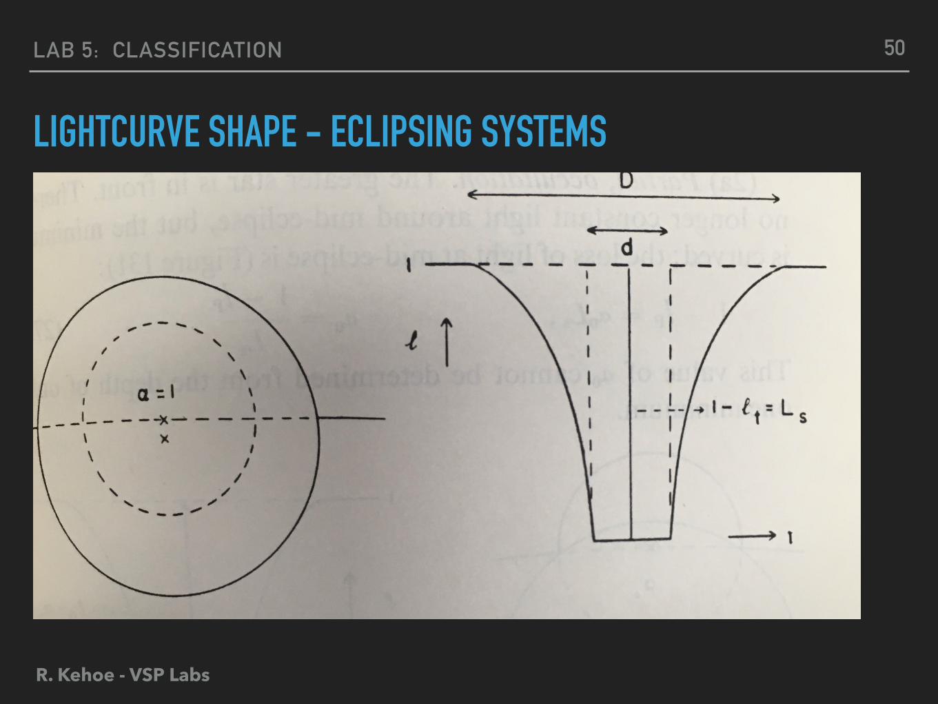
LIGHTCURVE SHAPE - ECLIPSING SYSTEMS

50

R. Kehoe - VSP Labs


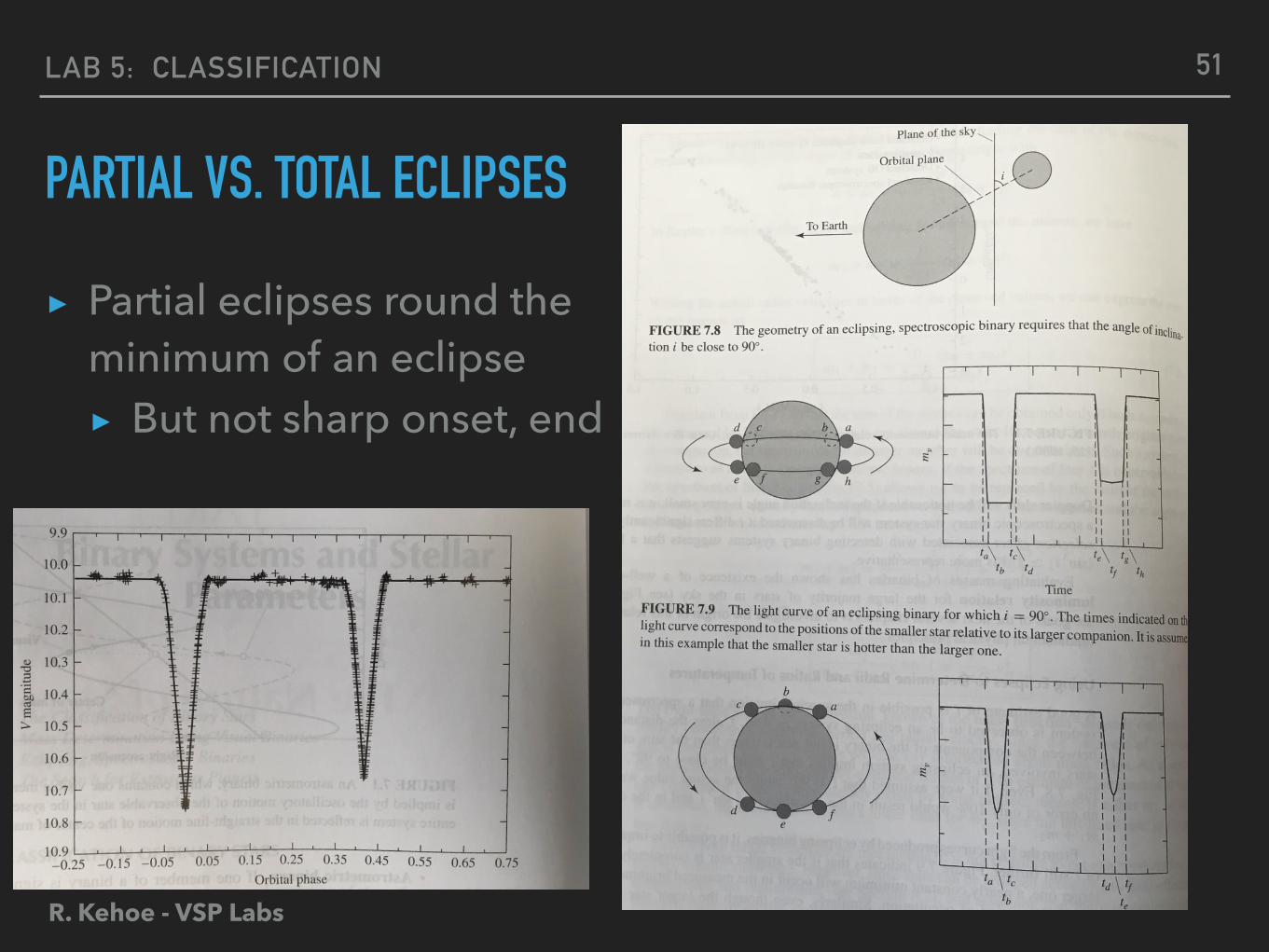
PARTIAL VS. TOTAL ECLIPSES

▸ Partial eclipses round the minimum of an eclipse ▸ But not sharp onset, end

51

R. Kehoe - VSP Labs


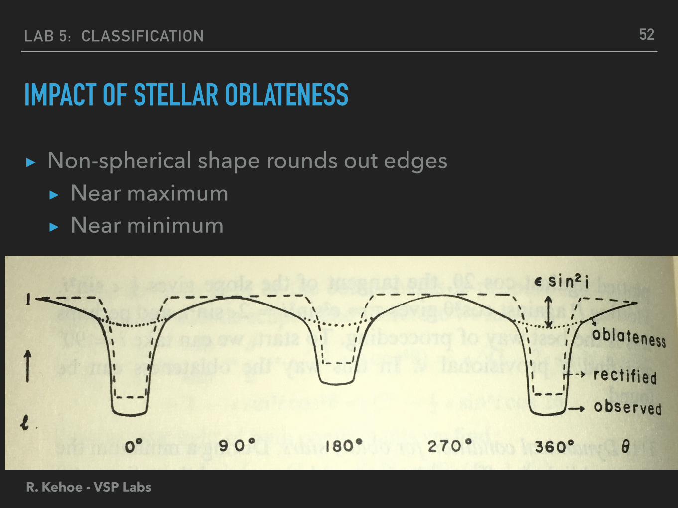
IMPACT OF STELLAR OBLATENESS

▸ Non-spherical shape rounds out edges ▸ Near maximum ▸ Near minimum

52

R. Kehoe - VSP Labs


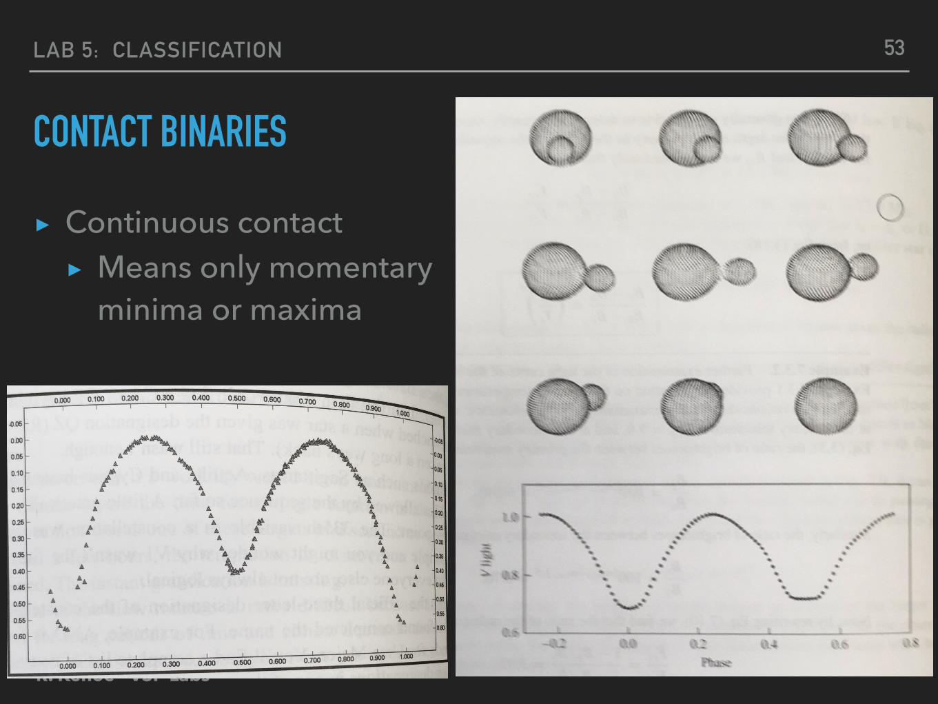
CONTACT BINARIES

▸ Continuous contact ▸ Means only momentary

minima or maxima

53

R. Kehoe - VSP Labs


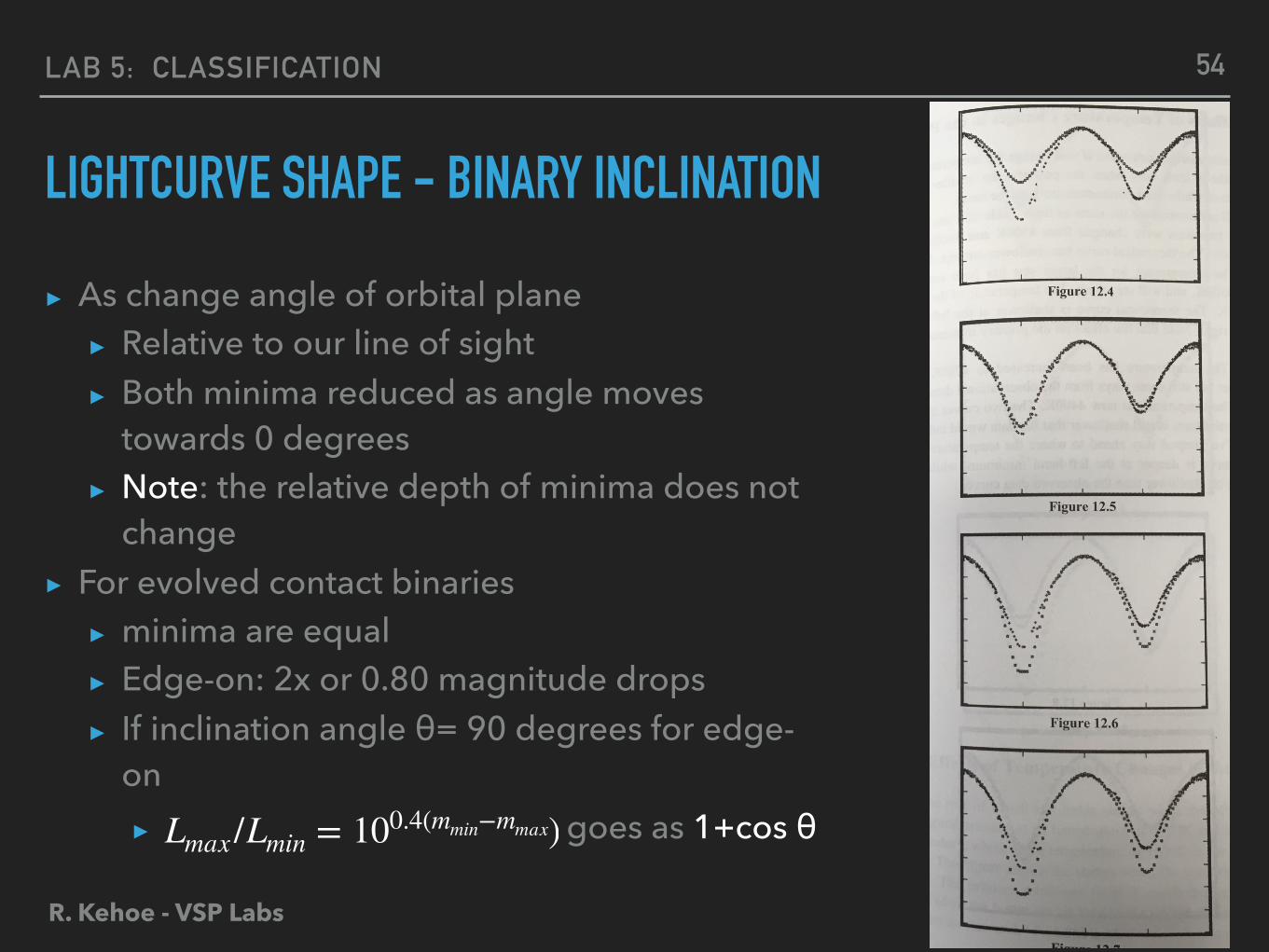
LIGHTCURVE SHAPE - BINARY INCLINATION

▸ As change angle of orbital plane ▸ Relative to our line of sight ▸ Both minima reduced as angle moves

towards 0 degrees ▸ Note: the relative depth of minima does not

change ▸ For evolved contact binaries

▸ minima are equal ▸ Edge-on: 2x or 0.80 magnitude drops ▸ If inclination angle θ= 90 degrees for edge-

on ▸ goes as 1+cos θLmax /Lmin = 100.4(mmin−mmax)

54

R. Kehoe - VSP Labs


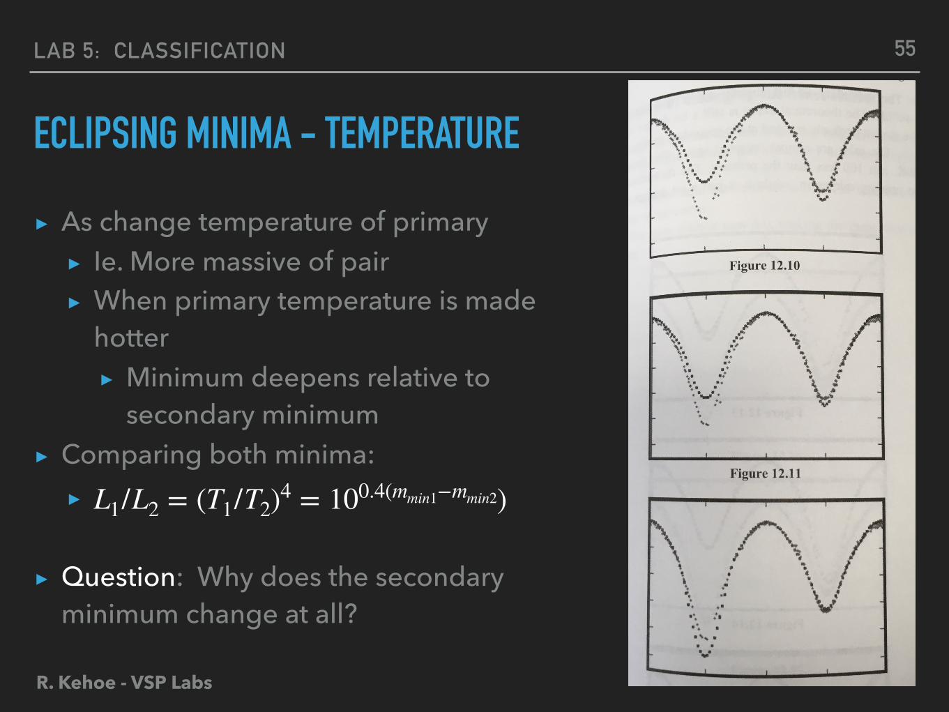
ECLIPSING MINIMA - TEMPERATURE

▸ As change temperature of primary ▸ Ie. More massive of pair ▸ When primary temperature is made

hotter ▸ Minimum deepens relative to

secondary minimum ▸ Comparing both minima: ▸

▸ Question: Why does the secondary minimum change at all?

L1/L2 = (T1/T2)4 = 100.4(mmin1−mmin2)

55

R. Kehoe - VSP Labs


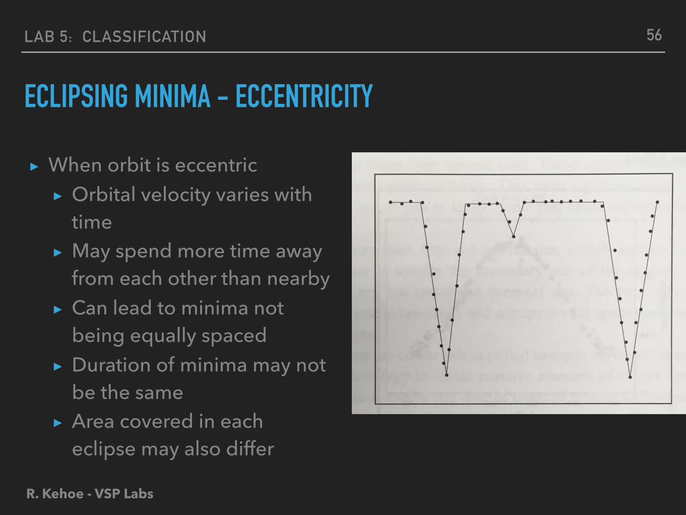
ECLIPSING MINIMA - ECCENTRICITY

▸ When orbit is eccentric ▸ Orbital velocity varies with

time ▸ May spend more time away

from each other than nearby ▸ Can lead to minima not

being equally spaced ▸ Duration of minima may not

be the same ▸ Area covered in each

eclipse may also differ

56

R. Kehoe - VSP Labs


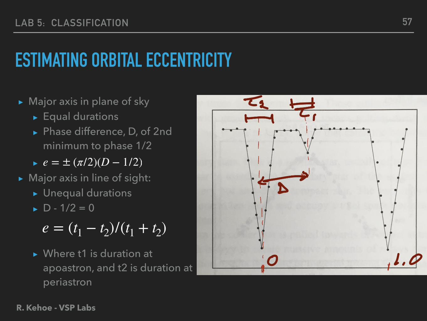
ESTIMATING ORBITAL ECCENTRICITY

▸ Major axis in plane of sky ▸ Equal durations ▸ Phase difference, D, of 2nd

minimum to phase 1/2 ▸

▸ Major axis in line of sight: ▸ Unequal durations ▸ D - 1/2 = 0

▸ Where t1 is duration at apoastron, and t2 is duration at periastron

e = ± (π/2)(D − 1/2)

57

e = (t1 − t2)/(t1 + t2)

R. Kehoe - VSP Labs


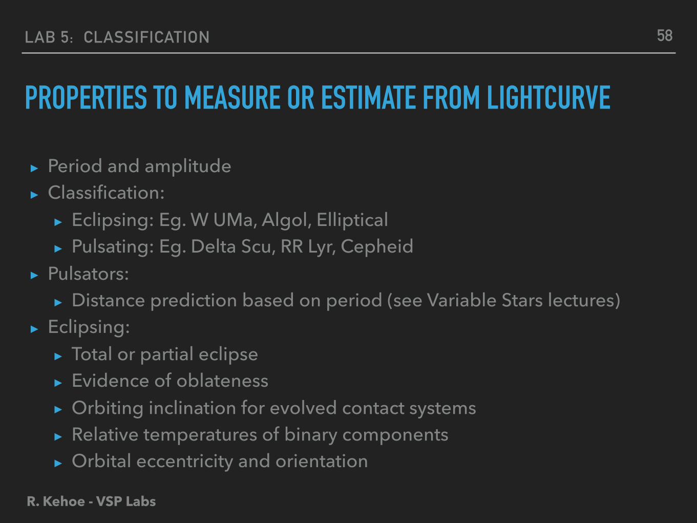
PROPERTIES TO MEASURE OR ESTIMATE FROM LIGHTCURVE

▸ Period and amplitude ▸ Classification:

▸ Eclipsing: Eg. W UMa, Algol, Elliptical ▸ Pulsating: Eg. Delta Scu, RR Lyr, Cepheid

▸ Pulsators: ▸ Distance prediction based on period (see Variable Stars lectures)

▸ Eclipsing: ▸ Total or partial eclipse ▸ Evidence of oblateness ▸ Orbiting inclination for evolved contact systems ▸ Relative temperatures of binary components ▸ Orbital eccentricity and orientation

58

R. Kehoe - VSP Labs


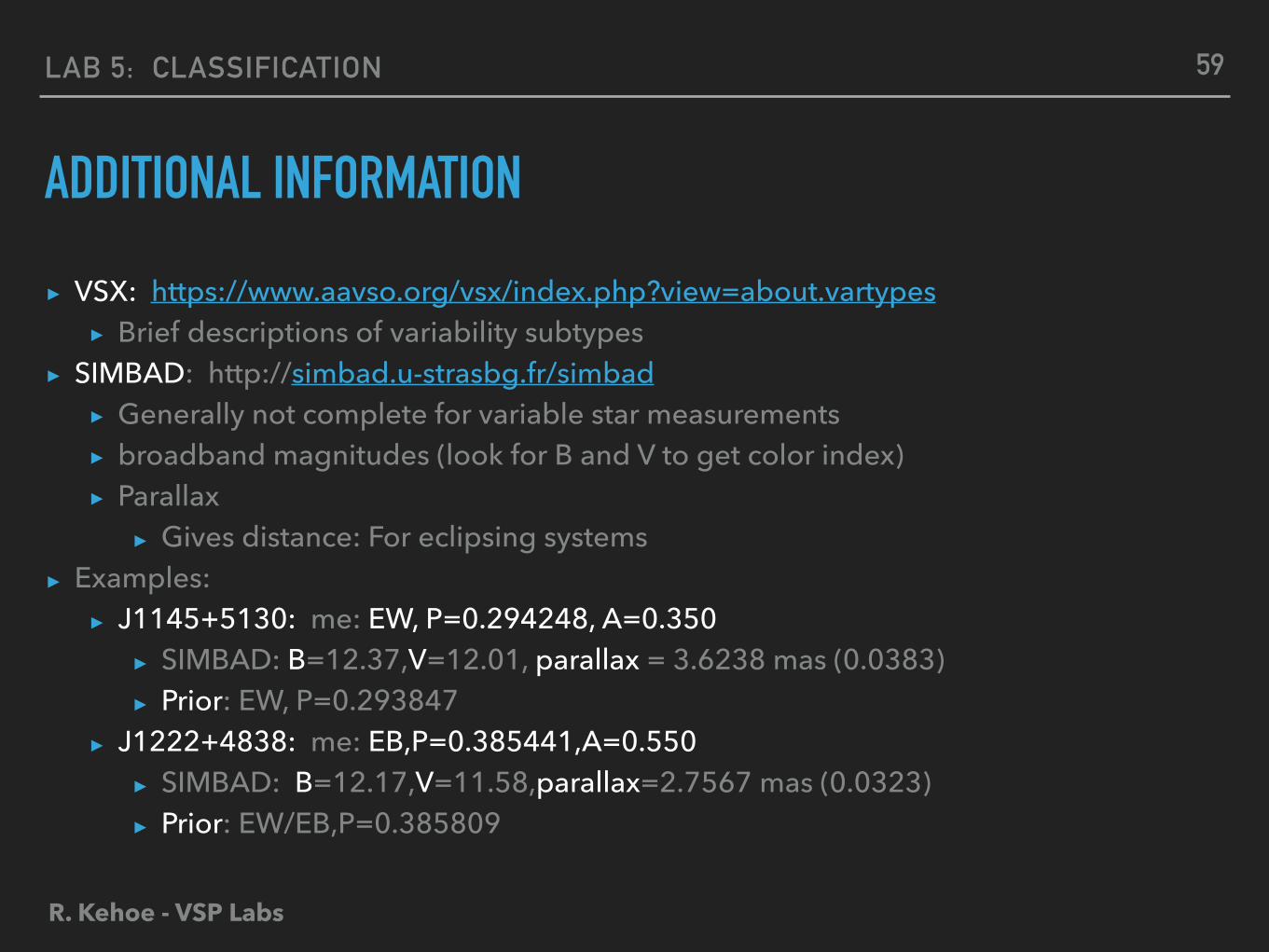
ADDITIONAL INFORMATION

▸ VSX: https://www.aavso.org/vsx/index.php?view=about.vartypes ▸ Brief descriptions of variability subtypes

▸ SIMBAD: http://simbad.u-strasbg.fr/simbad ▸ Generally not complete for variable star measurements ▸ broadband magnitudes (look for B and V to get color index) ▸ Parallax

▸ Gives distance: For eclipsing systems ▸ Examples:

▸ J1145+5130: me: EW, P=0.294248, A=0.350 ▸ SIMBAD: B=12.37,V=12.01, parallax = 3.6238 mas (0.0383) ▸ Prior: EW, P=0.293847

▸ J1222+4838: me: EB,P=0.385441,A=0.550 ▸ SIMBAD: B=12.17,V=11.58,parallax=2.7567 mas (0.0323) ▸ Prior: EW/EB,P=0.385809

59

https://www.aavso.org/vsx/index.php?view=about.vartypes

http://simbad.u-strasbg.fr/simbad

R. Kehoe - VSP Labs


FURTHER GUIDELINES FOR RESEARCH REPORTS▸ Always define acronyms and terms at first use ▸ Avoid text that does not contribute directly to your discussion of your thesis ▸ Avoid throw away lines or phrases, eg. “Things such as...” ▸ Utilize precise terminology when possible. Eg. ‘Graphs’ is not a clear term, ‘data

structures’ is clearer ▸ Avoid explaining basics from lecture - your audience is your peers. You should

demonstrate you know how to use the material from lecture and textbook. ▸ Avoid direct quotes from sources. Write out explicitly what you need in your paper in

your own words at the level you believe is at the level of your audience. When your points are part of a discussion in somebody else’s paper, you need to reference that source.

▸ Think carefully about appropriate order of material - eg. You may need to discuss the detector before you can adequately describe the data.

▸ Abstract: itemize key results, synopsis of important points of paper ▸ References Cited: should be primarily journal articles, although other primary sources

can supplement. Textbooks, and especially web pages, or discouraged, although the former are sometimes necessary for important points

60

Documents

LAB MATERIAL VARIABLE STARS PROJECT