Embed Size (px)
DESCRIPTION
This is the lab manual for using NetSim to cover the experiments of VTU MTECH course in adhoc networks
Citation preview
1
NetSimTM
Experiment Manual
2
The information contained in this document represents the current view of TETCOS on the
issues discussed as of the date of publication. Because TETCOS must respond to changing
market conditions, it should not be interpreted to be a commitment on the part of TETCOS, and
TETCOS cannot guarantee the accuracy of any information presented after the date of
publication.
This manual is for informational purposes only. TETCOS MAKES NO WARRANTIES,
EXPRESS, IMPLIED OR STATUTORY, AS TO THE INFORMATION IN THIS
DOCUMENT.
Warning! DO NOT COPY
Copyright in the whole and every part of this manual belongs to TETCOS and may not be used,
sold, transferred, copied or reproduced in whole or in part in any manner or in any media to any
person, without the prior written consent of TETCOS. If you use this manual you do so at your
own risk and on the understanding that TETCOS shall not be liable for any loss or damage of
any kind.
TETCOS may have patents, patent applications, trademarks, copyrights, or other intellectual
property rights covering subject matter in this document. Except as expressly provided in any
written license agreement from TETCOS, the furnishing of this document does not give you any
license to these patents, trademarks, copyrights, or other intellectual property. Unless otherwise
noted, the example companies, organizations, products, domain names, e-mail addresses, logos,
people, places, and events depicted herein are fictitious, and no association with any real
company, organization, product, domain name, email address, logo, person, place, or event is
intended or should be inferred.
Rev 8.2.4b1 (V), Jan 2015, TETCOS. All rights reserved.
All trademarks are property of their respective owner.
Contact us at –
TETCOS
214, 39th A Cross, 7th Main, 5th Block Jayanagar,
Bangalore - 560 041, Karnataka, INDIA. Phone: +91 80 26630624
E-Mail: [email protected]
Visit: www.tetcos.com
3
Simulation Experiments
1. Develop MAC Protocol using any suitable Network Simulator for MANETs to send the
packet without any contention through wireless link using the following MAC
protocols;(CSMA/CA (802.11)). Analyze its performance with increasing node density
and mobility. ……..( 4 )
2. Develop and Analyze
a. The performance of TCP connection when it is used for wireless networks You
will find performance of TCP decreases dramatically when a TCP connection
traverses a wireless link on which packets may be lost due to wireless
transmission errors.
b. Make use of Active Queue Management Technique to control congestion on
Wireless Networks and analyze performance of FIFO and WFQ over wireless
networks.
……..( 15 )
3. Simulate MANET environment using suitable Network Simulator and test with various
mobility model such as Random walk, Random way point and Group mobility. Analyze
throughput, PDR and delay with respect to different mobility models.
……..( 24 )
4. Develop unicast routing protocols using any suitable Network Simulator for (Mobile Ad
hoc Networks) MANET to find the best route using the any one of routing protocols from
each category from table-driven (e.g., OLSR) on demand (e.g., DSR, AODV), hybrid
(e.g., ZRP, contact-based architectures). Understand the advantages and disadvantages of
each routing protocol type by observing the performance metrics of the routing protocol.
……..( 32 )
4
Experiment 1
Objective: Develop MAC Protocol using any suitable Network Simulator for MANETs to send
the packet without any contention through wireless link using the following MAC
protocols;(CSMA/CA (802.11)). Analyze its performance with increasing node density and
mobility.
Introduction:
Mobile Ad-Hoc Network (MANET) is a self-configuring network of mobile nodes connected by
wireless links to form an arbitrary topology without the use of existing infrastructure. The nodes
are free to move randomly. Thus the network's wireless topology may be unpredictable and may
change rapidly.
Mobility and node density are the two major factors which influences the performance of any
routing protocol of mobile ad hoc network. The mobility of the nodes affects the number of
connected paths, which in turn affect the performance of the routing algorithm.
The node density also has an impact on the routing performance. With very sparsely populated
network the number of possible connection between any two nodes is very less and hence the
performance is poor. It is expected that if the node density is increased the throughput of the
network shall increase, but beyond a certain level if density is increased the performance
degrades.
Performance metrics:
The different parameters used to analyze the performance are explained as follows:
• Throughput: It is the rate of successfully transmitted data packets in unit time in the network
during the simulation.
• Average Delay: It is defined as the average time taken by the data packets to propagate from
source to destination across a MANET. This includes all possible delays caused by routing
discovery latency, queuing at the interface queue, and retransmission delays at the MAC,
propagation and transfer times.
5
• Packet Delivery Ration (PDR): This is the ratio of the number of data packets successfully
delivered to the destinations to those transmitted by sources.
Packet Delivery Ratio = Total_Packets_Received/ Total_Packets_Transmitted
Procedure:
How to Create Scenario & Generate Traffic:
• Create Scenario: Please refer “Help � NetSim Help � Running Simulation via
GUI�Advanced Wireless Networks �MANET �Create Scenario”.
Part A: Performance of a MANET network as node density is increased
Sample 1:
Step 1: Go to Simulation � New � Advanced Wireless Networks �MANET
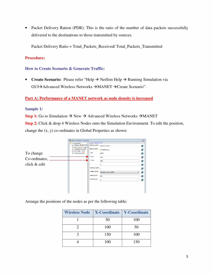
Step 2: Click & drop 4 Wireless Nodes onto the Simulation Environment. To edit the position,
change the (x, y) co-ordinates in Global Properties as shown:
Arrange the positions of the nodes as per the following table:
Wireless Node X-Coordinate Y-Coordinate
1 50 100
2 100 50
3 150 100
4 100 150
To change
Co-ordinates,
click & edit
6
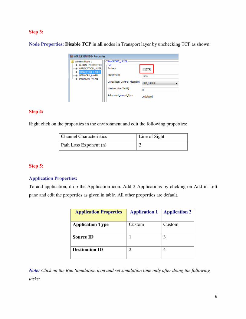
Step 3:
Node Properties: Disable TCP in all nodes in Transport layer by unchecking TCP as shown:
Step 4:
Right click on the properties in the environment and edit the following properties:
Channel Characteristics Line of Sight
Path Loss Exponent (n) 2
Step 5:
Application Properties:
To add application, drop the Application icon. Add 2 Applications by clicking on Add in Left
pane and edit the properties as given in table. All other properties are default.
Application Properties Application 1 Application 2
Application Type Custom Custom
Source ID 1 3
Destination ID 2 4
Note: Click on the Run Simulation icon and set simulation time only after doing the following
tasks:
7
• Set Environment properties,
• Set the properties of Nodes and
• Configure Applications.
Simulation Time- 100 Seconds
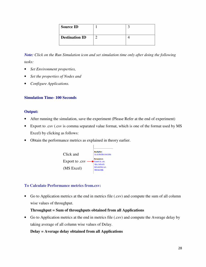
Output:
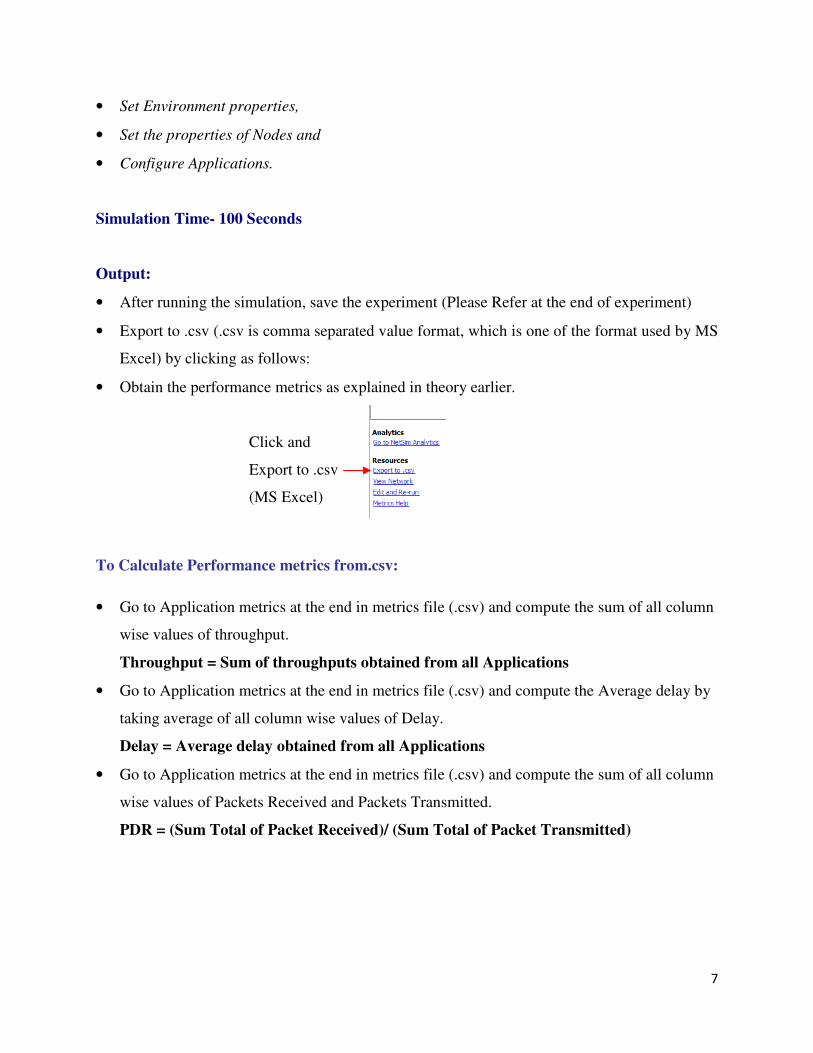
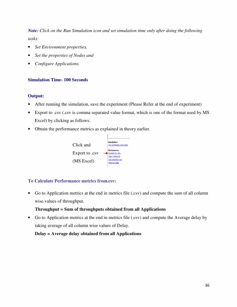
• After running the simulation, save the experiment (Please Refer at the end of experiment)
• Export to .csv (.csv is comma separated value format, which is one of the format used by MS
Excel) by clicking as follows:
• Obtain the performance metrics as explained in theory earlier.
To Calculate Performance metrics from.csv:
• Go to Application metrics at the end in metrics file (.csv) and compute the sum of all column
wise values of throughput.
Throughput = Sum of throughputs obtained from all Applications
• Go to Application metrics at the end in metrics file (.csv) and compute the Average delay by
taking average of all column wise values of Delay.
Delay = Average delay obtained from all Applications
• Go to Application metrics at the end in metrics file (.csv) and compute the sum of all column
wise values of Packets Received and Packets Transmitted.
PDR = (Sum Total of Packet Received)/ (Sum Total of Packet Transmitted)
Click and
Export to .csv
(MS Excel)
8
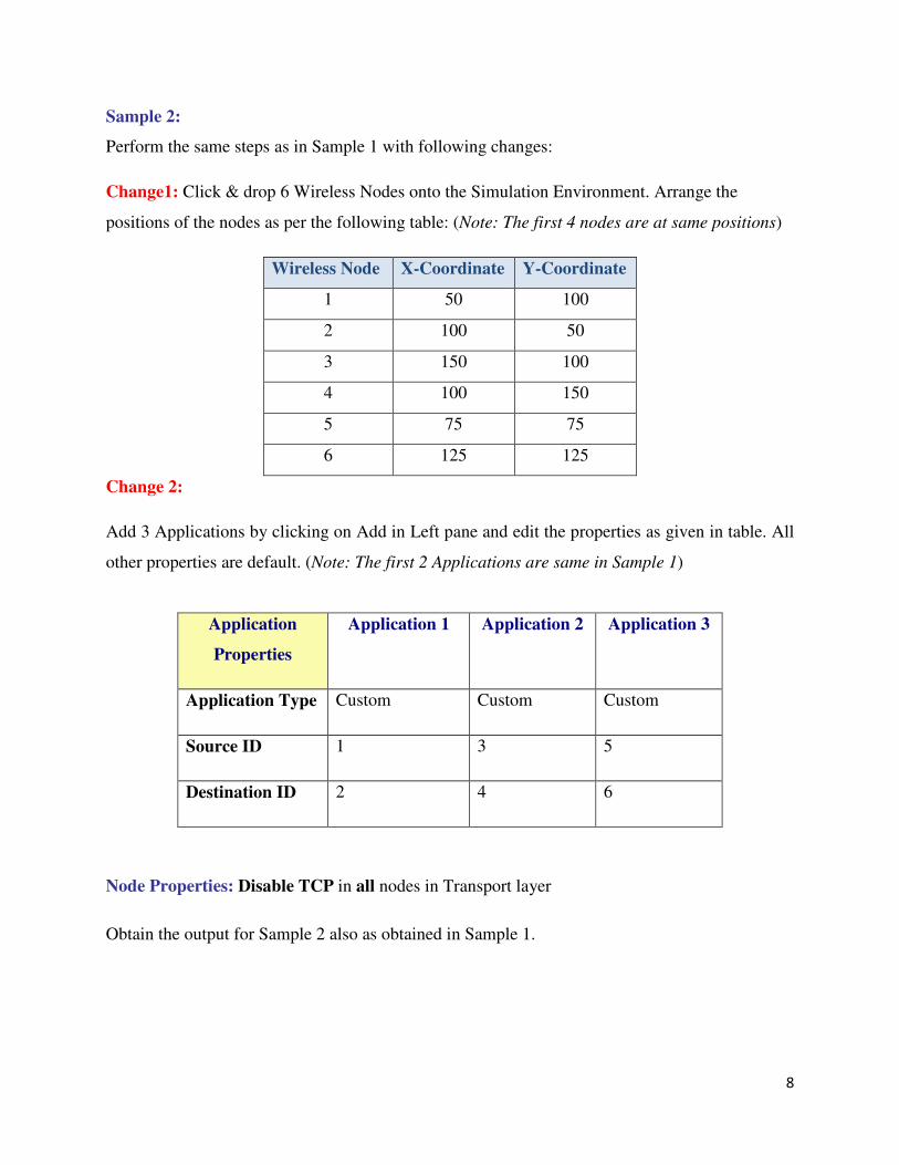
Sample 2:
Perform the same steps as in Sample 1 with following changes:
Change1: Click & drop 6 Wireless Nodes onto the Simulation Environment. Arrange the
positions of the nodes as per the following table: (Note: The first 4 nodes are at same positions)
Wireless Node X-Coordinate Y-Coordinate
1 50 100
2 100 50
3 150 100
4 100 150
5 75 75
6 125 125
Change 2:
Add 3 Applications by clicking on Add in Left pane and edit the properties as given in table. All
other properties are default. (Note: The first 2 Applications are same in Sample 1)
Application
Properties
Application 1 Application 2 Application 3
Application Type Custom Custom Custom
Source ID 1 3 5
Destination ID 2 4 6
Node Properties: Disable TCP in all nodes in Transport layer
Obtain the output for Sample 2 also as obtained in Sample 1.
9
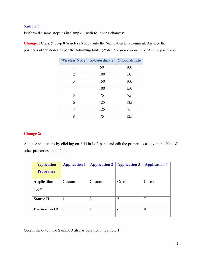
Sample 3:
Perform the same steps as in Sample 1 with following changes:
Change1: Click & drop 8 Wireless Nodes onto the Simulation Environment. Arrange the
positions of the nodes as per the following table: (Note: The first 6 nodes are at same positions)
Wireless Node X-Coordinate Y-Coordinate
1 50 100
2 100 50
3 150 100
4 100 150
5 75 75
6 125 125
7 125 75
8 75 125
Change 2:
Add 4 Applications by clicking on Add in Left pane and edit the properties as given in table. All
other properties are default.
Application
Properties
Application 1 Application 2 Application 3 Application 4
Application
Type
Custom Custom Custom Custom
Source ID 1 3 5 7
Destination ID 2 4 6 8
Obtain the output for Sample 3 also as obtained in Sample 1.
10
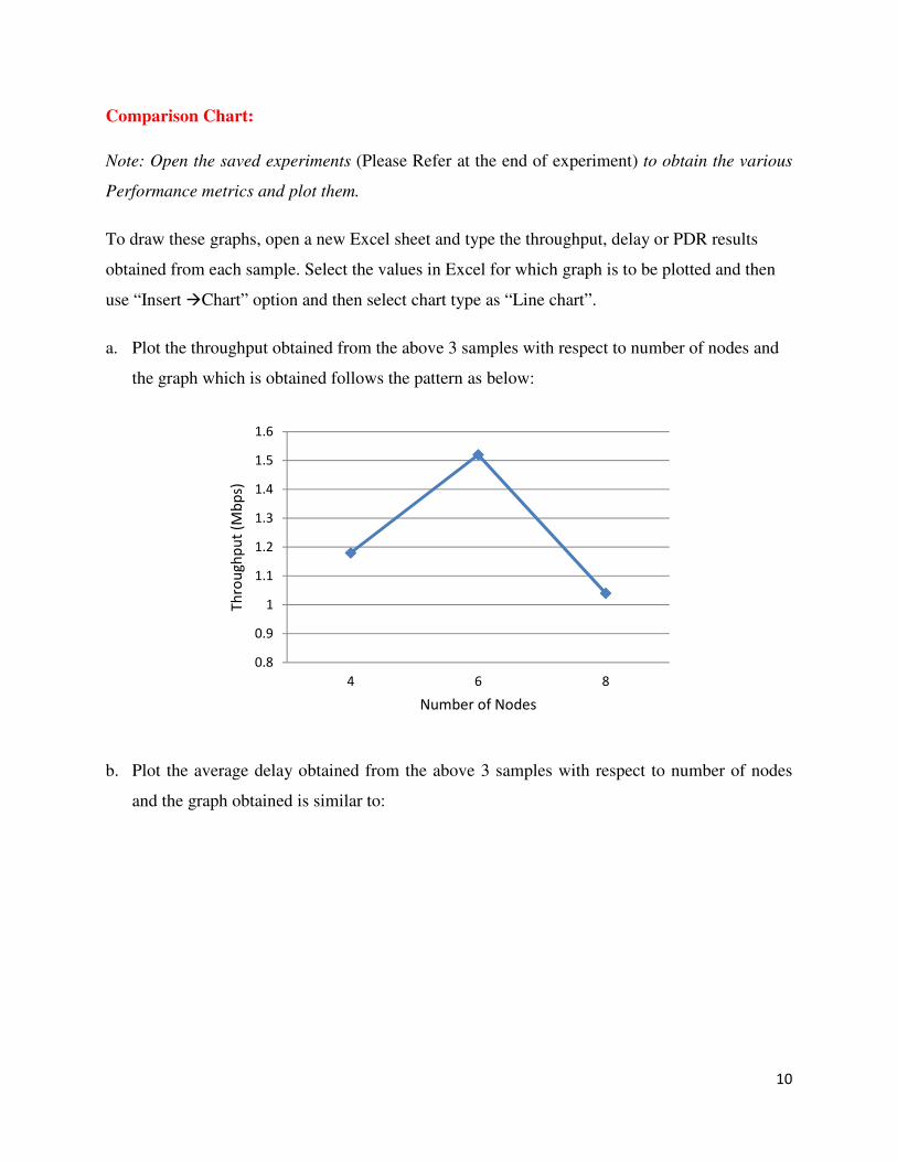
Comparison Chart:
Note: Open the saved experiments (Please Refer at the end of experiment) to obtain the various
Performance metrics and plot them.
To draw these graphs, open a new Excel sheet and type the throughput, delay or PDR results
obtained from each sample. Select the values in Excel for which graph is to be plotted and then
use “Insert �Chart” option and then select chart type as “Line chart”.
a. Plot the throughput obtained from the above 3 samples with respect to number of nodes and
the graph which is obtained follows the pattern as below:
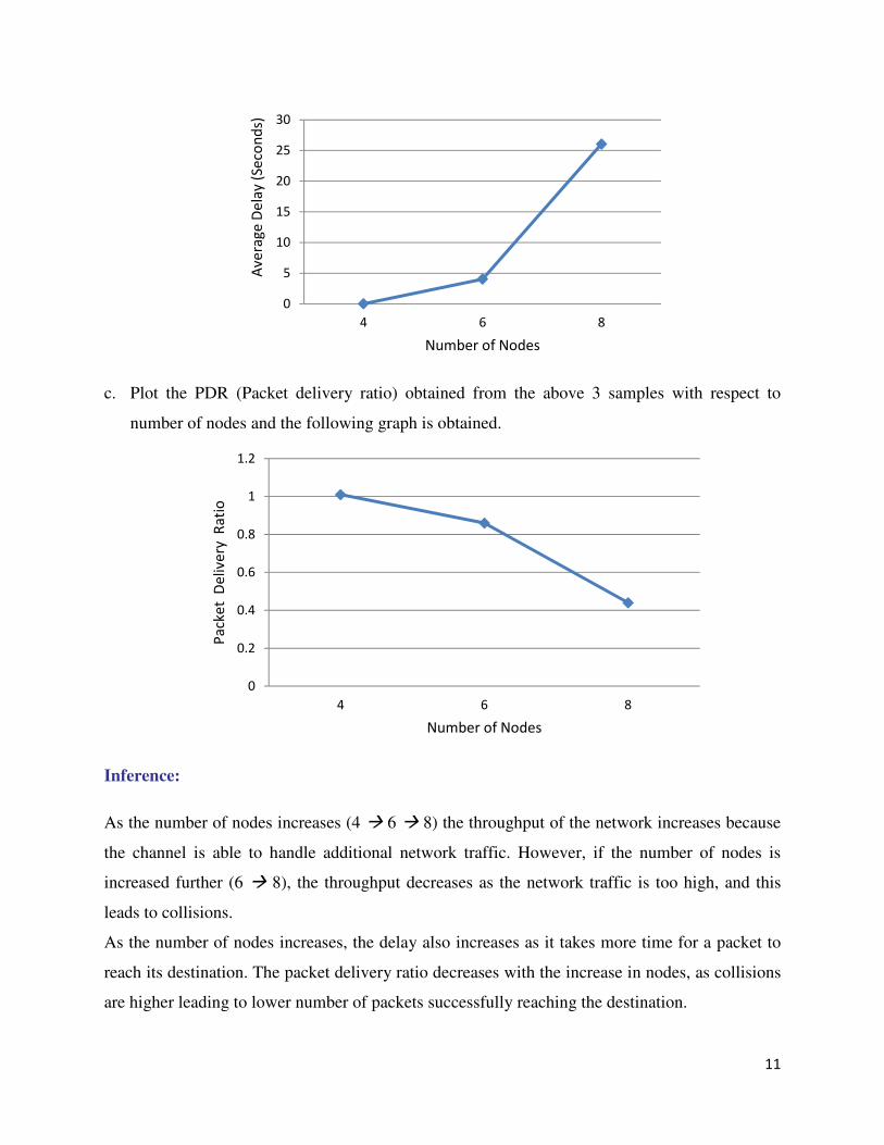
b. Plot the average delay obtained from the above 3 samples with respect to number of nodes
and the graph obtained is similar to:
0.8
0.9
1
1.1
1.2
1.3
1.4
1.5
1.6
4 6 8
Th
rou
gh
pu
t (M
bp
s)
Number of Nodes
11
c. Plot the PDR (Packet delivery ratio) obtained from the above 3 samples with respect to
number of nodes and the following graph is obtained.
Inference:
As the number of nodes increases (4 � 6 � 8) the throughput of the network increases because
the channel is able to handle additional network traffic. However, if the number of nodes is
increased further (6 � 8), the throughput decreases as the network traffic is too high, and this
leads to collisions.
As the number of nodes increases, the delay also increases as it takes more time for a packet to
reach its destination. The packet delivery ratio decreases with the increase in nodes, as collisions
are higher leading to lower number of packets successfully reaching the destination.
0
5
10
15
20
25
30
4 6 8
Av
era
ge
De
lay
(S
eco
nd
s)
Number of Nodes
0
0.2
0.4
0.6
0.8
1
1.2
4 6 8
Pa
cke
t D
eli
ve
ry R
ati
o
Number of Nodes
12
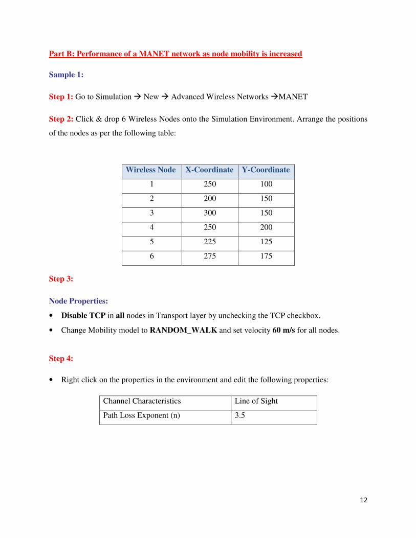
Part B: Performance of a MANET network as node mobility is increased
Sample 1:
Step 1: Go to Simulation � New � Advanced Wireless Networks �MANET
Step 2: Click & drop 6 Wireless Nodes onto the Simulation Environment. Arrange the positions
of the nodes as per the following table:
Wireless Node X-Coordinate Y-Coordinate
1 250 100
2 200 150
3 300 150
4 250 200
5 225 125
6 275 175
Step 3:
Node Properties:
• Disable TCP in all nodes in Transport layer by unchecking the TCP checkbox.
• Change Mobility model to RANDOM_WALK and set velocity 60 m/s for all nodes.
Step 4:
• Right click on the properties in the environment and edit the following properties:
Channel Characteristics Line of Sight
Path Loss Exponent (n) 3.5
13
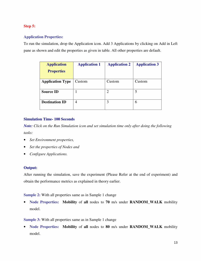
Step 5:
Application Properties:
To run the simulation, drop the Application icon. Add 3 Applications by clicking on Add in Left
pane as shown and edit the properties as given in table. All other properties are default.
Application
Properties
Application 1 Application 2 Application 3
Application Type Custom Custom Custom
Source ID 1 2 5
Destination ID 4 3 6
Simulation Time- 100 Seconds
Note: Click on the Run Simulation icon and set simulation time only after doing the following
tasks:
• Set Environment properties,
• Set the properties of Nodes and
• Configure Applications.
Output:
After running the simulation, save the experiment (Please Refer at the end of experiment) and
obtain the performance metrics as explained in theory earlier.
Sample 2: With all properties same as in Sample 1 change
• Node Properties: Mobility of all nodes to 70 m/s under RANDOM_WALK mobility
model.
Sample 3: With all properties same as in Sample 1 change
• Node Properties: Mobility of all nodes to 80 m/s under RANDOM_WALK mobility
model.
14
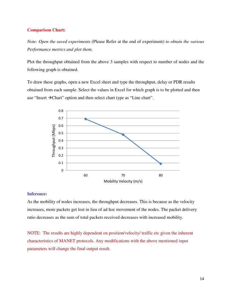
Comparison Chart:
Note: Open the saved experiments (Please Refer at the end of experiment) to obtain the various
Performance metrics and plot them.
Plot the throughput obtained from the above 3 samples with respect to number of nodes and the
following graph is obtained.
To draw these graphs, open a new Excel sheet and type the throughput, delay or PDR results
obtained from each sample. Select the values in Excel for which graph is to be plotted and then
use “Insert �Chart” option and then select chart type as “Line chart”.
Inference:
As the mobility of nodes increases, the throughput decreases. This is because as the velocity
increases, more packets get lost in lieu of ad hoc movement of the nodes. The packet delivery
ratio decreases as the sum of total packets received decreases with increased mobility.
NOTE: The results are highly dependent on position/velocity/ traffic etc given the inherent
characteristics of MANET protocols. Any modifications with the above mentioned input
parameters will change the final output result.
0
0.1
0.2
0.3
0.4
0.5
0.6
0.7
0.8
60 70 80
Th
rou
gh
pu
t (M
bp
s)
Mobility Velocity (m/s)
15
Experiment 2
Objective: Develop and Analyze
1. The performance of TCP connection when it is used for wireless networks You will find
performance of TCP decreases dramatically when a TCP connection traverses a wireless
link on which packets may be lost due to wireless transmission errors.
2. Make use of Active Queue Management Technique to control congestion on Wireless
Networks and analyze performance of FIFO and WFQ over wireless networks.
Introduction:
Mobile Ad-Hoc Network (MANET) is a self-configuring network of mobile nodes connected by
wireless links to form an arbitrary topology without the use of existing infrastructure. The nodes
are free to move randomly. Thus the network's wireless topology may be unpredictable and may
change rapidly.
In MANETs, random wireless errors and mobility serves as primary contributor to losses as well
as congestion. More than 80% of the losses in the network are due to link failures. Essentially,
most losses in ad-hoc networks occur as a result of route failures
TCP uses the occurrence of losses to detect congestion. If TCP enters congestion control state
because of packet losses caused by random wireless errors and mobility, then the throughput of
TCP can be degraded significantly.
TCP maintains a congestion window, which is an estimate of the number of packets that can be
in transit without causing congestion. The congestion window starts at one packet, with new
acknowledgments causing it to be incremented by one, thus doubling after each RTT. This is the
slow start phase (exponential increase). When a loss is detected by a timeout, slow start threshold
is then set to half the value of the congestion window, the congestion window is reset to one
packet, and the lost packet is retransmitted.
Subsequently, in the congestion avoidance phase (linear increase), the congestion window is
incremented by one packet per RTT. When losses are detected by duplicate acknowledgments,
16
indicating that subsequent packets have been received, TCP retransmits the lost packet, halves
the congestion window, and restarts with the congestion avoidance phase. The TCP assumption
that all losses are due to congestion becomes quite problematic over wireless links. Multiple
losses may repeatedly reduce the slow start threshold, causing the slower congestion avoidance
phase to take over immediately, leading to large throughput degradations.
The IEEE 802.11 is a set of media access control (MAC) and physical layer (PHY) specifications
for implementing wireless network. The 802.11 MAC works with a single first-in-first-out
(FIFO) transmission queue while 802.11e MAC has multiple transmission queues, where each
queue maintains its own Backoff Counter.
First-in, first-out (FIFO) queuing is the most basic queue scheduling discipline. In FIFO queuing,
all packets are treated equally by placing them into a single queue, and then servicing them in the
same order that they were placed into the queue. FIFO queuing is also referred to as First-come,
first-served (FCFS) queuing.
Weighted fair queueing (WFQ) is a data packet scheduling technique allowing different
scheduling priorities to statistically multiplexed data flows.
Performance metrics:
The parameter used to analyze the performance are explained as follows:
• Throughput: It is the rate of successfully transmitted data packets in unit time in the network
during the simulation.
Procedure:
How to Create Scenario & Generate Traffic:
Please refer,
• Create Scenario: “Help � NetSim Help � Running Simulation via GUI�Advanced
Wireless Networks �MANET �Create Scenario”.
17
Part 1: Sample 1:
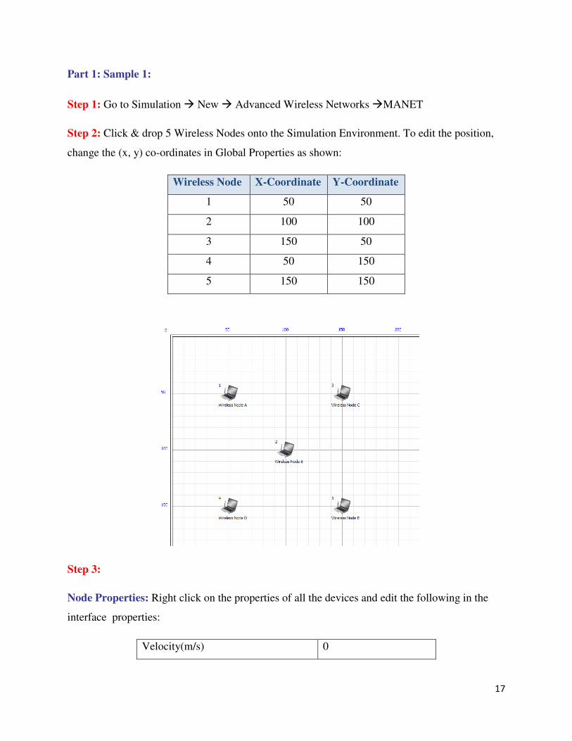
Step 1: Go to Simulation � New � Advanced Wireless Networks �MANET
Step 2: Click & drop 5 Wireless Nodes onto the Simulation Environment. To edit the position,
change the (x, y) co-ordinates in Global Properties as shown:
Wireless Node X-Coordinate Y-Coordinate
1 50 50
2 100 100
3 150 50
4 50 150
5 150 150
Step 3:
Node Properties: Right click on the properties of all the devices and edit the following in the
interface properties:
Velocity(m/s) 0
18
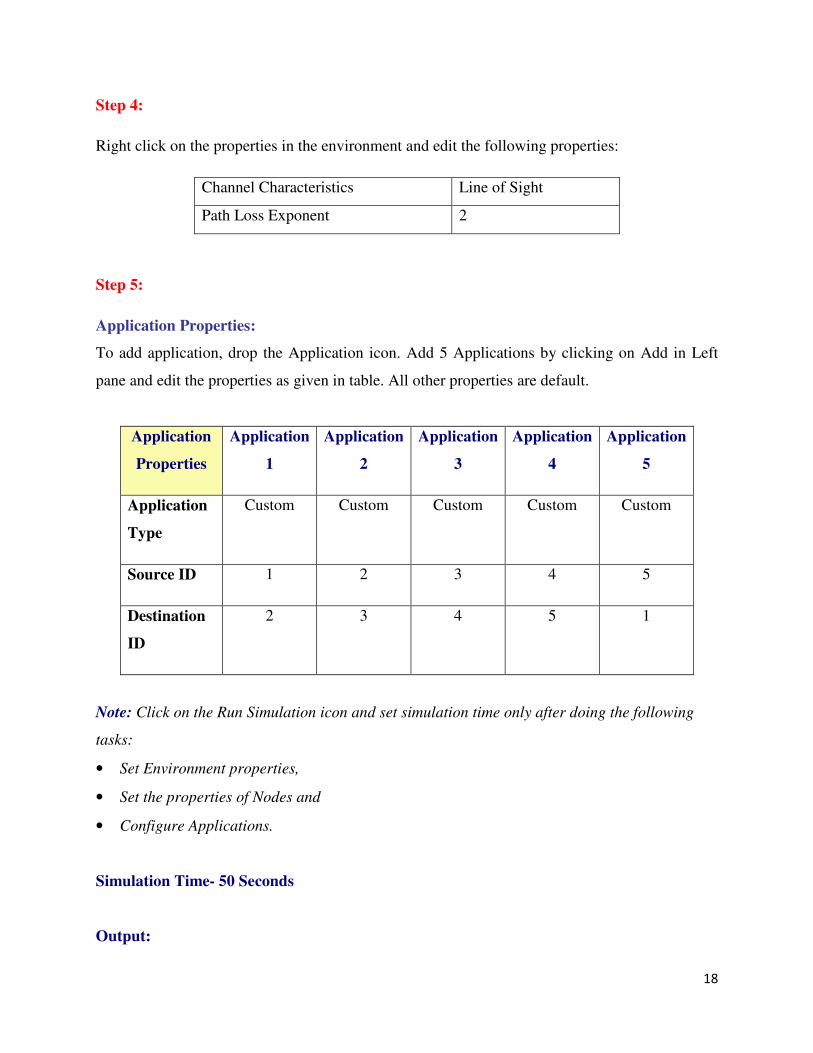
Step 4:
Right click on the properties in the environment and edit the following properties:
Channel Characteristics Line of Sight
Path Loss Exponent 2
Step 5:
Application Properties:
To add application, drop the Application icon. Add 5 Applications by clicking on Add in Left
pane and edit the properties as given in table. All other properties are default.
Application
Properties
Application
1
Application
2
Application
3
Application
4
Application
5
Application
Type
Custom Custom Custom Custom Custom
Source ID 1 2 3 4 5
Destination
ID
2 3 4 5 1
Note: Click on the Run Simulation icon and set simulation time only after doing the following
tasks:
• Set Environment properties,
• Set the properties of Nodes and
• Configure Applications.
Simulation Time- 50 Seconds
Output:
19
• After running the simulation, save the experiment (Please Refer at the end of experiment).
• Export to .csv by clicking on left pane in metrics window.
• Obtain the performance metrics as explained in theory earlier.
To Calculate Performance metrics from.csv:
• Go to Application metrics at the end in metrics file (.csv) and compute the sum of all column
wise values of throughput.
Throughput = Sum of throughputs obtained from all Applications
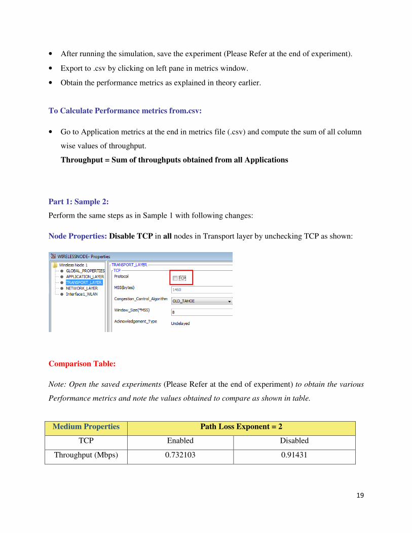
Part 1: Sample 2:
Perform the same steps as in Sample 1 with following changes:
Node Properties: Disable TCP in all nodes in Transport layer by unchecking TCP as shown:
Comparison Table:
Note: Open the saved experiments (Please Refer at the end of experiment) to obtain the various
Performance metrics and note the values obtained to compare as shown in table.
Medium Properties Path Loss Exponent = 2
TCP Enabled Disabled
Throughput (Mbps) 0.732103 0.91431
20
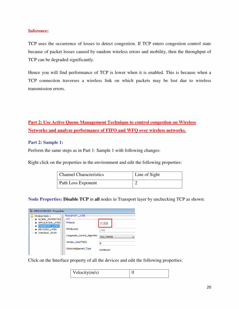
Inference:
TCP uses the occurrence of losses to detect congestion. If TCP enters congestion control state
because of packet losses caused by random wireless errors and mobility, then the throughput of
TCP can be degraded significantly.
Hence you will find performance of TCP is lower when it is enabled. This is because when a
TCP connection traverses a wireless link on which packets may be lost due to wireless
transmission errors.
Part 2: Use Active Queue Management Technique to control congestion on Wireless
Networks and analyze performance of FIFO and WFQ over wireless networks.
Part 2: Sample 1:
Perform the same steps as in Part 1: Sample 1 with following changes:
Right click on the properties in the environment and edit the following properties:
Channel Characteristics Line of Sight
Path Loss Exponent 2
Node Properties: Disable TCP in all nodes in Transport layer by unchecking TCP as shown:
Click on the Interface property of all the devices and edit the following properties:
Velocity(m/s) 0
21
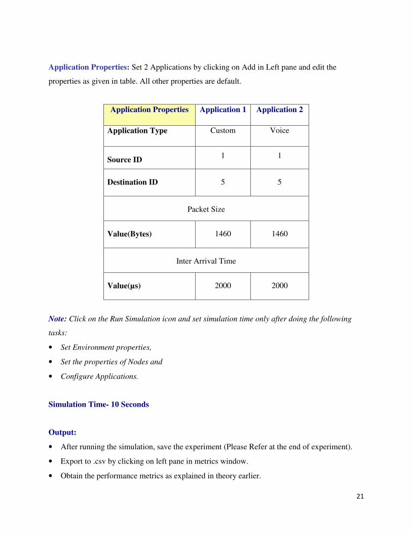
Application Properties: Set 2 Applications by clicking on Add in Left pane and edit the
properties as given in table. All other properties are default.
Application Properties Application 1 Application 2
Application Type Custom Voice
Source ID 1 1
Destination ID 5 5
Packet Size
Value(Bytes) 1460 1460
Inter Arrival Time
Value(µs) 2000 2000
Note: Click on the Run Simulation icon and set simulation time only after doing the following
tasks:
• Set Environment properties,
• Set the properties of Nodes and
• Configure Applications.
Simulation Time- 10 Seconds
Output:
• After running the simulation, save the experiment (Please Refer at the end of experiment).
• Export to .csv by clicking on left pane in metrics window.
• Obtain the performance metrics as explained in theory earlier.
22
To Calculate Performance metrics from.csv:
• Go to Application metrics at the end in metrics file (.csv) and compute the sum of all column
wise values of throughput.
Throughput = Sum of throughputs obtained from all Applications
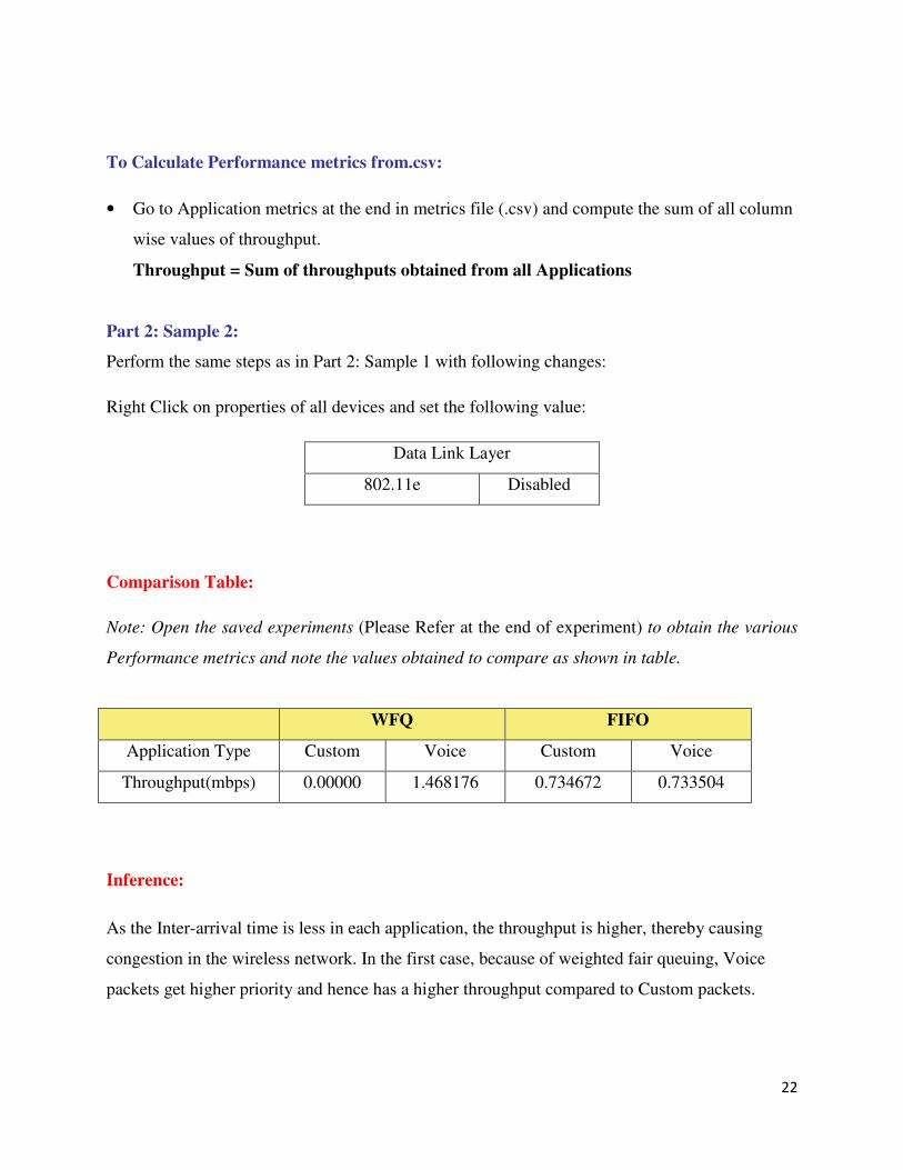
Part 2: Sample 2:
Perform the same steps as in Part 2: Sample 1 with following changes:
Right Click on properties of all devices and set the following value:
Data Link Layer
802.11e Disabled
Comparison Table:
Note: Open the saved experiments (Please Refer at the end of experiment) to obtain the various
Performance metrics and note the values obtained to compare as shown in table.
WFQ FIFO
Application Type Custom Voice Custom Voice
Throughput(mbps) 0.00000 1.468176 0.734672 0.733504
Inference:
As the Inter-arrival time is less in each application, the throughput is higher, thereby causing
congestion in the wireless network. In the first case, because of weighted fair queuing, Voice
packets get higher priority and hence has a higher throughput compared to Custom packets.
23
But in the second case, because of FIFO(First-in-First-out), equal number of both Voice and
Custom packets are transmitted, thereby having same throughput.
NOTE: The results are highly dependent on position/velocity/ traffic etc given the inherent
characteristics of MANET protocols. Any modifications with the above mentioned input
parameters will change the final output result.
24
Experiment 3
Objective: Simulate MANET environment using suitable Network Simulator and test with
various mobility model such as Random walk, Random way point and Group mobility. Analyze
throughput, PDR and delay with respect to different mobility models.
Introduction:
Mobile Ad-Hoc Network (MANET) is a self-configuring network of mobile nodes connected by
wireless links to form an arbitrary topology without the use of existing infrastructure. The
movement of the nodes can be defined by various mobility models like Random walk, Random
way point and Group mobility .
Random walk: In this mobility model, a mobile node moves from its current location to a new
location by randomly choosing a direction and speed in which to travel. Each movement in the
Random Walk Mobility Model occurs in either a constant time interval t or a constant
traveled d distance, at the end of which a new direction and speed are calculated.
Random way point: The Random Way Point Mobility Model includes pauses between changes
in direction and/or speed. A Mobile node begins by staying in one location for a certain period of
time (i.e pause). Once this time expires, the mobile node chooses a random destination in the
simulation area. The mobile node then travels toward the newly chosen destination at the
selected speed. Upon arrival, the mobile node pauses for a specified period of time starting the
process again.
Group mobility: In case of Group Mobility, the mobile nodes belonging to the same group will
move with same properties i.e velocity and direction.
Performance metrics:
The different parameters used to analyze the performance are explained as follows:
25
• Throughput: It is the rate of successfully transmitted data packets in unit time in the network
during the simulation.
• Average Delay: It is defined as the average time taken by the data packets to propagate from
source to destination across a MANET. This includes all possible delays caused by routing
discovery latency, queuing at the interface queue, and retransmission delays at the MAC,
propagation and transfer times.
• Packet Delivery Ration (PDR): This is the ratio of the number of data packets successfully
delivered to the destinations to those transmitted by sources.
Packet Delivery Ratio = Total_Packets_Received/ Total_Packets_Transmitted
Procedure:
How to Create Scenario & Generate Traffic:
• Create Scenario: Please refer “Help � NetSim Help � Running Simulation via
GUI�Advanced Wireless Networks �MANET �Create Scenario”.
Sample 1:
Step 1: Go to Simulation � New � Advanced Wireless Networks �MANET
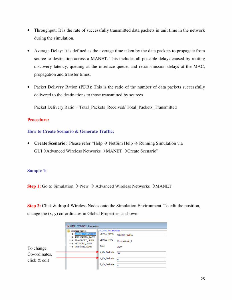
Step 2: Click & drop 4 Wireless Nodes onto the Simulation Environment. To edit the position,
change the (x, y) co-ordinates in Global Properties as shown:
To change
Co-ordinates,
click & edit
26
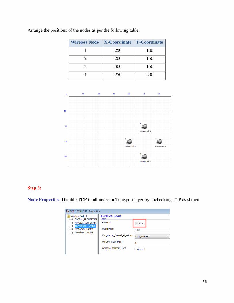
Arrange the positions of the nodes as per the following table:
Wireless Node X-Coordinate Y-Coordinate
1 250 100
2 200 150
3 300 150
4 250 200
Step 3:
Node Properties: Disable TCP in all nodes in Transport layer by unchecking TCP as shown:
27
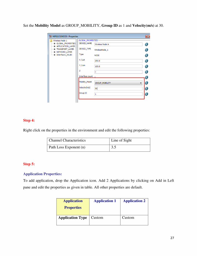
Set the Mobility Model as GROUP_MOBILITY, Group ID as 1 and Velocity(m/s) at 30.
Step 4:
Right click on the properties in the environment and edit the following properties:
Channel Characteristics Line of Sight
Path Loss Exponent (n) 3.5
Step 5:
Application Properties:
To add application, drop the Application icon. Add 2 Applications by clicking on Add in Left
pane and edit the properties as given in table. All other properties are default.
Application
Properties
Application 1 Application 2
Application Type Custom Custom
28
Source ID 1 3
Destination ID 2 4
Note: Click on the Run Simulation icon and set simulation time only after doing the following
tasks:
• Set Environment properties,
• Set the properties of Nodes and
• Configure Applications.
Simulation Time- 100 Seconds
Output:
• After running the simulation, save the experiment (Please Refer at the end of experiment)
• Export to .csv (.csv is comma separated value format, which is one of the format used by MS
Excel) by clicking as follows:
• Obtain the performance metrics as explained in theory earlier.
To Calculate Performance metrics from.csv:
• Go to Application metrics at the end in metrics file (.csv) and compute the sum of all column
wise values of throughput.
Throughput = Sum of throughputs obtained from all Applications
• Go to Application metrics at the end in metrics file (.csv) and compute the Average delay by
taking average of all column wise values of Delay.
Delay = Average delay obtained from all Applications
Click and
Export to .csv
(MS Excel)
29
• Go to Application metrics at the end in metrics file (.csv) and compute the sum of all column
wise values of Packets Received and Packets Transmitted.
PDR = (Sum Total of Packet Received)/ (Sum Total of Packet Transmitted)
Sample 2:
Perform the same steps as in Sample 1 with following changes:
Change 1: Node Properties:
Set the Mobility Model as RANDOM_WAY_POINT and Velocity(m/s) at 30.
Obtain the output for Sample 2 also as obtained in Sample 1.
Sample 3:
Perform the same steps as in Sample 1 with following changes:
Change 1: Node Properties:
Set the Mobility Model as RANDOM_WALK and Velocity(m/s) at 30.
Obtain the output for Sample 3 also as obtained in Sample 1.
Comparison Chart:
Note: Open the saved experiments (Please Refer at the end of experiment) to obtain the various
Performance metrics and plot them.
To draw these graphs, open a new Excel sheet and type the throughput, delay or PDR results
obtained from each sample. Select the values in Excel for which graph is to be plotted and then
use “Insert �Chart” option and then select chart type as “Line chart”.
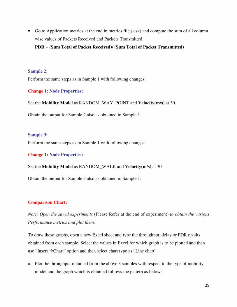
a. Plot the throughput obtained from the above 3 samples with respect to the type of mobility
model and the graph which is obtained follows the pattern as below:
30
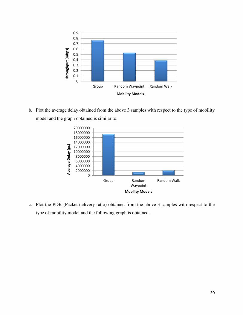
b. Plot the average delay obtained from the above 3 samples with respect to the type of mobility
model and the graph obtained is similar to:
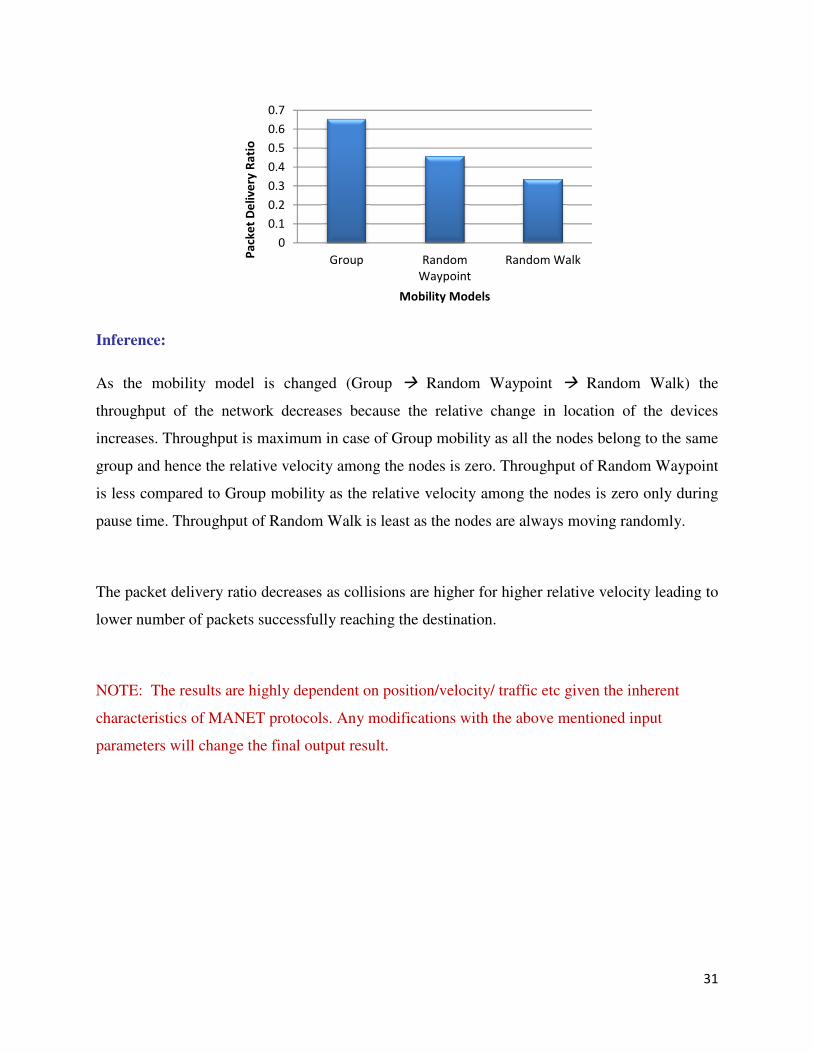
c. Plot the PDR (Packet delivery ratio) obtained from the above 3 samples with respect to the
type of mobility model and the following graph is obtained.
0
0.1
0.2
0.3
0.4
0.5
0.6
0.7
0.8
0.9
Group Random Waypoint Random Walk
Th
rou
gh
pu
t (m
bp
s)
Mobility Models
0
2000000
4000000
6000000
8000000
10000000
12000000
14000000
16000000
18000000
20000000
Group Random
Waypoint
Random Walk
Av
era
ge
De
lay
(µ
s)
Mobility Models
31
Inference:
As the mobility model is changed (Group � Random Waypoint � Random Walk) the
throughput of the network decreases because the relative change in location of the devices
increases. Throughput is maximum in case of Group mobility as all the nodes belong to the same
group and hence the relative velocity among the nodes is zero. Throughput of Random Waypoint
is less compared to Group mobility as the relative velocity among the nodes is zero only during
pause time. Throughput of Random Walk is least as the nodes are always moving randomly.
The packet delivery ratio decreases as collisions are higher for higher relative velocity leading to
lower number of packets successfully reaching the destination.
NOTE: The results are highly dependent on position/velocity/ traffic etc given the inherent
characteristics of MANET protocols. Any modifications with the above mentioned input
parameters will change the final output result.
0
0.1
0.2
0.3
0.4
0.5
0.6
0.7
Group Random
Waypoint
Random WalkPa
cke
t D
eli
ve
ry R
ati
o
Mobility Models
32
Experiment 4
Objective: Develop unicast routing protocols using any suitable Network Simulator for (Mobile
Ad hoc Networks) MANET to find the best route using the any one of routing protocols from
each category from table-driven (e.g., OLSR- optimized link state routing) on demand (e.g.,
DSR, AODV), hybrid (e.g., ZRP). Understand the advantages and disadvantages of each routing
protocol type by observing the performance metrics of the routing protocol.
Introduction: The various kinds of unicast routing protocols available in MANET are
Table-driven (proactive) routing: This type of protocols maintains fresh lists of destinations
and their routes by periodically distributing routing tables throughout the network. The main
disadvantages of such algorithms are:
1. Respective amount of data for maintenance.
2. Slow reaction on restructuring and failures.
Examples of proactive algorithms are: Optimized Link State Routing Protocol (OLSR).
On-demand (reactive) routing: This type of protocols finds a route on demand by flooding the
network with Route Request packets. The main disadvantages of such algorithms are:
1. High latency time in route finding.
2. Excessive flooding can lead to network clogging.
Examples of on-demand algorithms are: Ad hoc On-demand Distance Vector(AODV),Dynamic
Source Routing
Hybrid (both proactive and reactive) routing: This type of protocol combines the advantages
of proactive and reactive routing. The routing is initially established with some proactively
prospected routes and then serves the demand from additionally activated nodes through reactive
flooding. The choice of one or the other method requires predetermination for typical cases. The
main disadvantages of such algorithms are:
1. Advantage depends on number of other nodes activated.
2. Reaction to traffic demand depends on gradient of traffic volume.
33
Examples of hybrid algorithms are: ZRP (Zone Routing Protocol)
Performance metrics:
The different parameters used to analyze the performance are explained as follows:
• Throughput: It is the rate of successfully transmitted data packets in unit time in the network
during the simulation.
• Average Delay: It is defined as the average time taken by the data packets to propagate from
source to destination across a MANET. This includes all possible delays caused by routing
discovery latency, queuing at the interface queue, and retransmission delays at the MAC,
propagation and transfer times.
Procedure:
How to Create Scenario & Generate Traffic:
• Create Scenario: Please refer “Help � NetSim Help � Running Simulation via
GUI�Advanced Wireless Networks �MANET �Create Scenario”.
Sample 1:
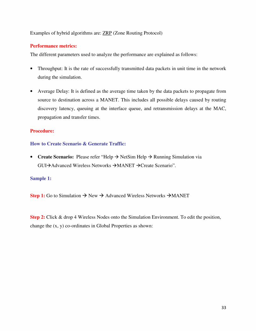
Step 1: Go to Simulation � New � Advanced Wireless Networks �MANET
Step 2: Click & drop 4 Wireless Nodes onto the Simulation Environment. To edit the position,
change the (x, y) co-ordinates in Global Properties as shown:
34
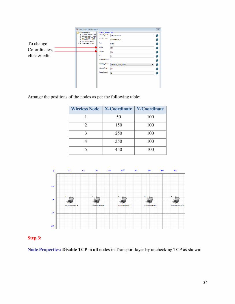
Arrange the positions of the nodes as per the following table:
Wireless Node X-Coordinate Y-Coordinate
1 50 100
2 150 100
3 250 100
4 350 100
5 450 100
Step 3:
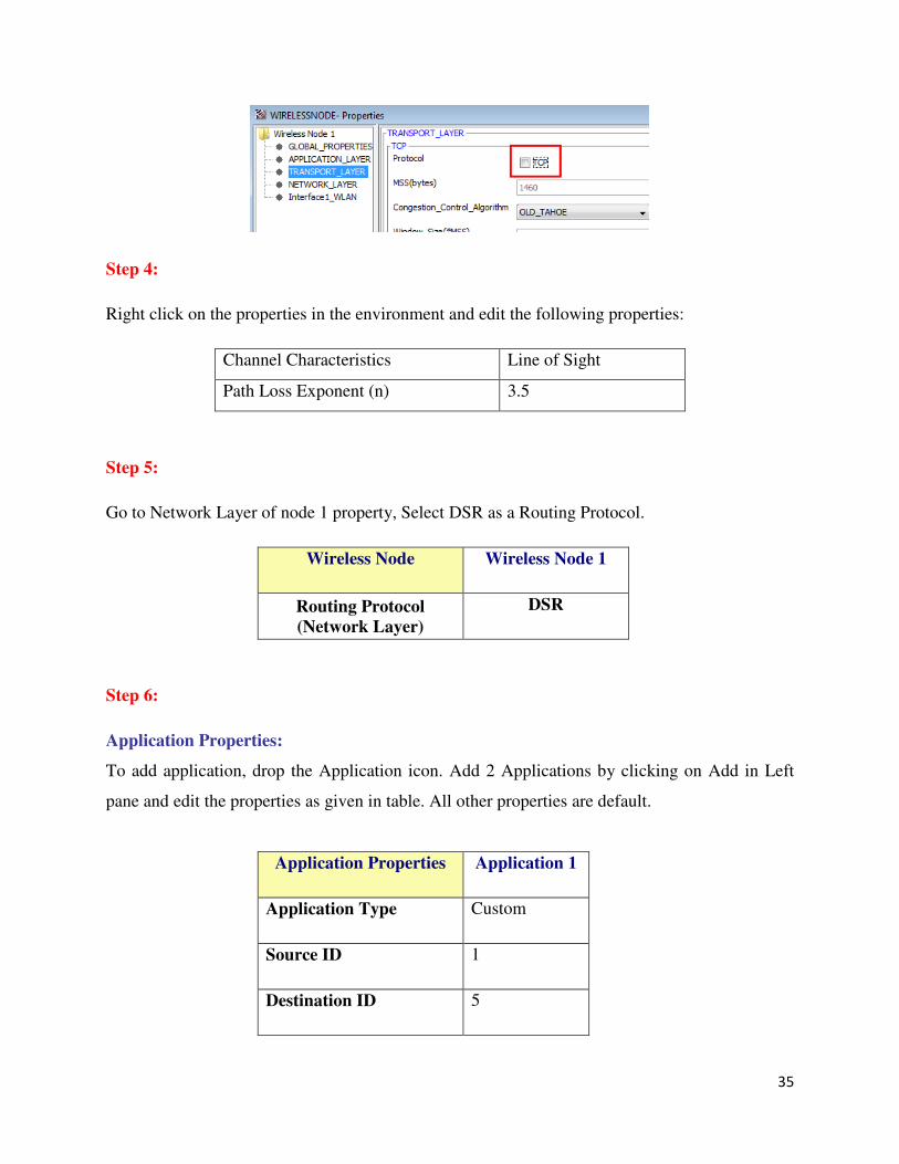
Node Properties: Disable TCP in all nodes in Transport layer by unchecking TCP as shown:
To change
Co-ordinates,
click & edit
35
Step 4:
Right click on the properties in the environment and edit the following properties:
Channel Characteristics Line of Sight
Path Loss Exponent (n) 3.5
Step 5:
Go to Network Layer of node 1 property, Select DSR as a Routing Protocol.
Wireless Node Wireless Node 1
Routing Protocol
(Network Layer)
DSR
Step 6:
Application Properties:
To add application, drop the Application icon. Add 2 Applications by clicking on Add in Left
pane and edit the properties as given in table. All other properties are default.
Application Properties Application 1
Application Type Custom
Source ID 1
Destination ID 5
36
Note: Click on the Run Simulation icon and set simulation time only after doing the following
tasks:
• Set Environment properties,
• Set the properties of Nodes and
• Configure Applications.
Simulation Time- 100 Seconds
Output:
• After running the simulation, save the experiment (Please Refer at the end of experiment)
• Export to .csv (.csv is comma separated value format, which is one of the format used by MS
Excel) by clicking as follows:
• Obtain the performance metrics as explained in theory earlier.
To Calculate Performance metrics from.csv:
• Go to Application metrics at the end in metrics file (.csv) and compute the sum of all column
wise values of throughput.
Throughput = Sum of throughputs obtained from all Applications
• Go to Application metrics at the end in metrics file (.csv) and compute the Average delay by
taking average of all column wise values of Delay.
Delay = Average delay obtained from all Applications
Click and
Export to .csv
(MS Excel)
37
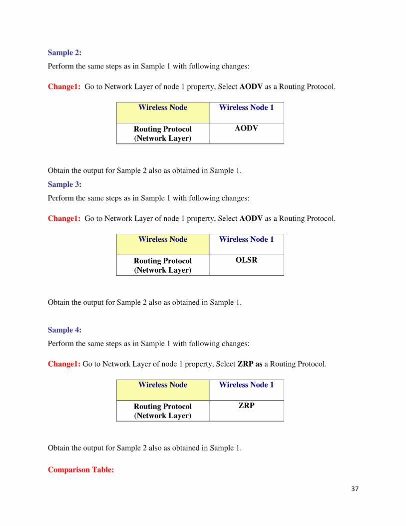
Sample 2:
Perform the same steps as in Sample 1 with following changes:
Change1: Go to Network Layer of node 1 property, Select AODV as a Routing Protocol.
Wireless Node Wireless Node 1
Routing Protocol
(Network Layer)
AODV
Obtain the output for Sample 2 also as obtained in Sample 1.
Sample 3:
Perform the same steps as in Sample 1 with following changes:
Change1: Go to Network Layer of node 1 property, Select AODV as a Routing Protocol.
Wireless Node Wireless Node 1
Routing Protocol
(Network Layer)
OLSR
Obtain the output for Sample 2 also as obtained in Sample 1.
Sample 4:
Perform the same steps as in Sample 1 with following changes:
Change1: Go to Network Layer of node 1 property, Select ZRP as a Routing Protocol.
Wireless Node Wireless Node 1
Routing Protocol
(Network Layer)
ZRP
Obtain the output for Sample 2 also as obtained in Sample 1.
Comparison Table:
38
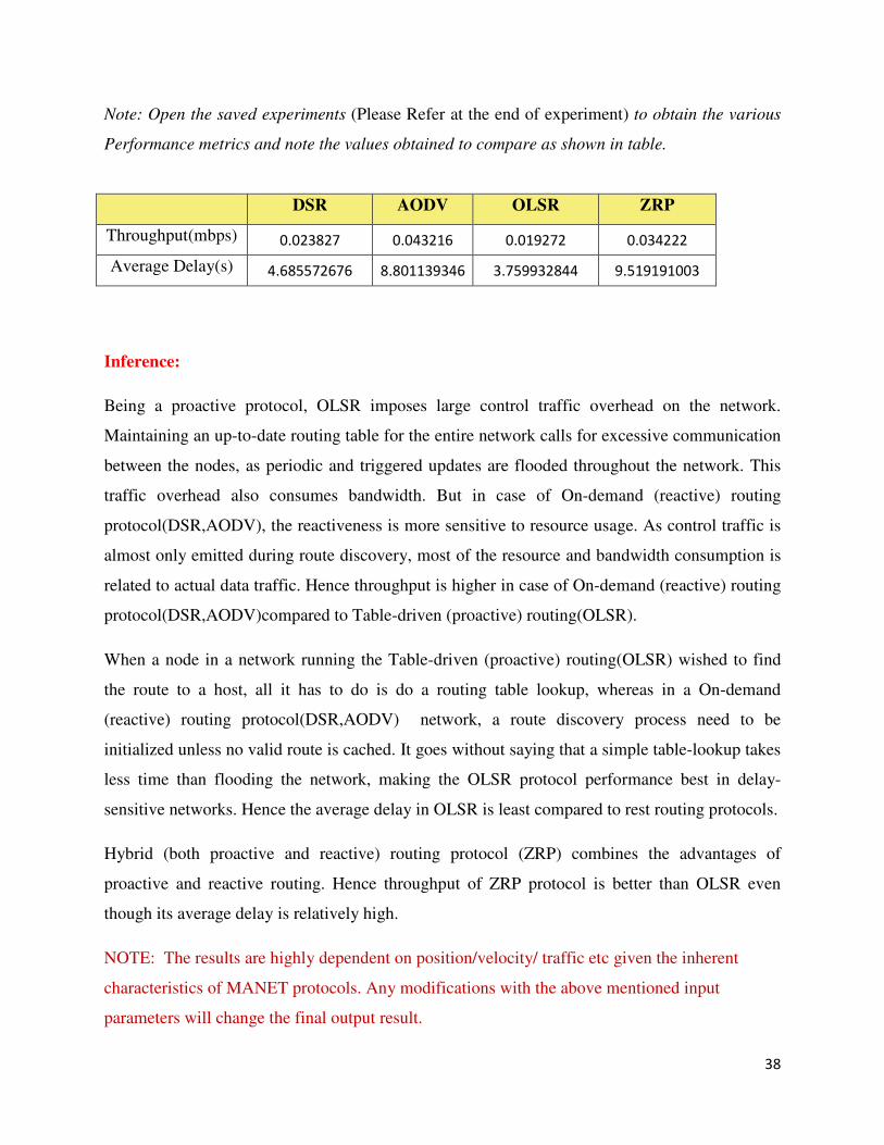
Note: Open the saved experiments (Please Refer at the end of experiment) to obtain the various
Performance metrics and note the values obtained to compare as shown in table.
DSR AODV OLSR ZRP
Throughput(mbps) 0.023827 0.043216 0.019272 0.034222
Average Delay(s) 4.685572676 8.801139346 3.759932844 9.519191003
Inference:
Being a proactive protocol, OLSR imposes large control traffic overhead on the network.
Maintaining an up-to-date routing table for the entire network calls for excessive communication
between the nodes, as periodic and triggered updates are flooded throughout the network. This
traffic overhead also consumes bandwidth. But in case of On-demand (reactive) routing
protocol(DSR,AODV), the reactiveness is more sensitive to resource usage. As control traffic is
almost only emitted during route discovery, most of the resource and bandwidth consumption is
related to actual data traffic. Hence throughput is higher in case of On-demand (reactive) routing
protocol(DSR,AODV)compared to Table-driven (proactive) routing(OLSR).
When a node in a network running the Table-driven (proactive) routing(OLSR) wished to find
the route to a host, all it has to do is do a routing table lookup, whereas in a On-demand
(reactive) routing protocol(DSR,AODV) network, a route discovery process need to be
initialized unless no valid route is cached. It goes without saying that a simple table-lookup takes
less time than flooding the network, making the OLSR protocol performance best in delay-
sensitive networks. Hence the average delay in OLSR is least compared to rest routing protocols.
Hybrid (both proactive and reactive) routing protocol (ZRP) combines the advantages of
proactive and reactive routing. Hence throughput of ZRP protocol is better than OLSR even
though its average delay is relatively high.
NOTE: The results are highly dependent on position/velocity/ traffic etc given the inherent
characteristics of MANET protocols. Any modifications with the above mentioned input
parameters will change the final output result.
39
How to Save and Open Saved Experiment (Help):
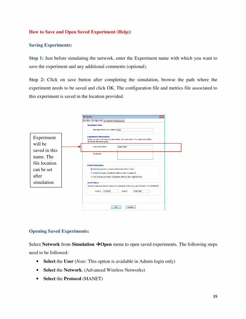
Saving Experiments:
Step 1: Just before simulating the network, enter the Experiment name with which you want to
save the experiment and any additional comments (optional).
Step 2: Click on save button after completing the simulation, browse the path where the
experiment needs to be saved and click OK. The configuration file and metrics file associated to
this experiment is saved in the location provided.
Opening Saved Experiments:
Select Network from Simulation ����Open menu to open saved experiments. The following steps
need to be followed:
• Select the User (Note: This option is available in Admin login only)
• Select the Network. (Advanced Wireless Networks)
• Select the Protocol (MANET)
Experiment
will be
saved in this
name. The
file location
can be set
after
simulation

40
• Select the Config File of the particular Experiment that needs to be opened using
Browse button.
• Click on Ok button to open the specified Experiment. User can modify the existing
Scenario, Simulate and Save it. Else Click on Cancel button to Exit the screen.