Embed Size (px)
Citation preview

Lab Manual for EE380 (Control Lab)Department of Electrical Engineering, IIT Kanpur
Manavaalan Gunasekaran and Ramprasad Potluri
Lab Manual Version: September 26, 2011

September 26, 2011 EE380 (Control Lab) IITK Lab Manual
ii

Contents
Preface vii0.1 Skills the control experiments need to impart . . . . . . . . . . . vii0.2 Past status of Control Systems Laboratory . . . . . . . . . . . . . vii
0.2.1 Logistical challenges . . . . . . . . . . . . . . . . . . . . . viii0.2.2 Solution to these challenges . . . . . . . . . . . . . . . . . viii
0.3 Planning for the future . . . . . . . . . . . . . . . . . . . . . . . . viii0.3.1 Models for the experiments . . . . . . . . . . . . . . . . . viii0.3.2 Suggested new set of experiments . . . . . . . . . . . . . ix0.3.3 Skills the pmdc motor control experiments help develop x
Contributions to the lab xi
1 The experimental setup 11.1 Introduction . . . . . . . . . . . . . . . . . . . . . . . . . . . . . . 11.2 Microcontroller dsPIC30F4012 . . . . . . . . . . . . . . . . . . . . 1
1.2.1 Timer Module . . . . . . . . . . . . . . . . . . . . . . . . . 21.2.2 Pulse Width Modulation (PWM) Module . . . . . . . . . 21.2.3 Quadrature Encoder Interface (QEI) Module . . . . . . . 21.2.4 Universal Asynchronous Receiver Transmitter (UART)
Module . . . . . . . . . . . . . . . . . . . . . . . . . . . . . 41.2.5 GPIO Pins . . . . . . . . . . . . . . . . . . . . . . . . . . . 41.2.6 Analog to Digital Convertor (ADC) . . . . . . . . . . . . 4
1.3 Choice of sampling interval . . . . . . . . . . . . . . . . . . . . . 41.4 Characteristics of the H-bridge board . . . . . . . . . . . . . . . . 5
1.4.1 Calculation of B . . . . . . . . . . . . . . . . . . . . . . . . 61.4.2 Motor armature resistance . . . . . . . . . . . . . . . . . . 71.4.3 Mismatch between practical and theoretical responses . 7
1.5 Programming . . . . . . . . . . . . . . . . . . . . . . . . . . . . . 71.5.1 Reading the data from dsPIC to PC . . . . . . . . . . . . 8
1.6 Parameters of DC motor-gear-encoder unit . . . . . . . . . . . . 81.7 Program listings . . . . . . . . . . . . . . . . . . . . . . . . . . . . 8
1.7.1 main-prog.c . . . . . . . . . . . . . . . . . . . . . . . . . . 81.7.2 settings-prog.h . . . . . . . . . . . . . . . . . . . . . . . . 121.7.3 readplot.m . . . . . . . . . . . . . . . . . . . . . . . . . . . 15
1.8 Schematic of the dsPIC30F4012 board . . . . . . . . . . . . . . . 19
iii
September 26, 2011 EE380 (Control Lab) IITK Lab Manual
2 Experiment 1: PMDC motor modeling, identification, speed control 212.1 Goals . . . . . . . . . . . . . . . . . . . . . . . . . . . . . . . . . . 212.2 Introduction . . . . . . . . . . . . . . . . . . . . . . . . . . . . . . 212.3 Exercises . . . . . . . . . . . . . . . . . . . . . . . . . . . . . . . . 21
2.3.1 To do at home . . . . . . . . . . . . . . . . . . . . . . . . . 212.3.2 To do in lab . . . . . . . . . . . . . . . . . . . . . . . . . . 22
2.4 Physics-based model of the DC motor unit . . . . . . . . . . . . 222.5 System identification . . . . . . . . . . . . . . . . . . . . . . . . . 232.6 Discretized version of the controller . . . . . . . . . . . . . . . . 24
2.6.1 Conversion from transfer function to state-space . . . . . 242.6.2 Discretization of the state-space equation . . . . . . . . . 262.6.3 Time-domain recursion . . . . . . . . . . . . . . . . . . . 26
2.7 Simulation . . . . . . . . . . . . . . . . . . . . . . . . . . . . . . . 262.8 Program listings . . . . . . . . . . . . . . . . . . . . . . . . . . . . 27
2.8.1 easysim.m . . . . . . . . . . . . . . . . . . . . . . . . . . . 27
3 Experiment 2: Speed of pmdc motor tracks reference sinusoid 293.1 Goals . . . . . . . . . . . . . . . . . . . . . . . . . . . . . . . . . . 293.2 Dead zone in the Vm versus u characteristic . . . . . . . . . . . . 293.3 Questions . . . . . . . . . . . . . . . . . . . . . . . . . . . . . . . 30
3.3.1 To do at home . . . . . . . . . . . . . . . . . . . . . . . . . 303.3.2 To do in lab . . . . . . . . . . . . . . . . . . . . . . . . . . 30
3.4 System identification . . . . . . . . . . . . . . . . . . . . . . . . . 323.5 Program listings . . . . . . . . . . . . . . . . . . . . . . . . . . . . 32
3.5.1 sysid.m . . . . . . . . . . . . . . . . . . . . . . . . . . . . . 323.5.2 simsine.m . . . . . . . . . . . . . . . . . . . . . . . . . . . 34
4 Experiment 3: Ziegler-Nichols tuning of speed controller of pmdc mo-tor 374.1 Goals . . . . . . . . . . . . . . . . . . . . . . . . . . . . . . . . . . 374.2 What is controller tuning? . . . . . . . . . . . . . . . . . . . . . . 374.3 What the two ZNT methods do . . . . . . . . . . . . . . . . . . . 384.4 First method . . . . . . . . . . . . . . . . . . . . . . . . . . . . . . 384.5 Second method . . . . . . . . . . . . . . . . . . . . . . . . . . . . 394.6 A modification of the plant . . . . . . . . . . . . . . . . . . . . . 404.7 Questions . . . . . . . . . . . . . . . . . . . . . . . . . . . . . . . 40
4.7.1 To do at home . . . . . . . . . . . . . . . . . . . . . . . . . 404.7.2 To do in lab: Second ZNT method . . . . . . . . . . . . . 42
5 Experiment 4: Control of speed using armature current 435.1 Goals . . . . . . . . . . . . . . . . . . . . . . . . . . . . . . . . . . 435.2 Application of this problem . . . . . . . . . . . . . . . . . . . . . 435.3 Background . . . . . . . . . . . . . . . . . . . . . . . . . . . . . . 445.4 Questions . . . . . . . . . . . . . . . . . . . . . . . . . . . . . . . 45
5.4.1 To do at home . . . . . . . . . . . . . . . . . . . . . . . . . 455.4.2 To do in lab . . . . . . . . . . . . . . . . . . . . . . . . . . 46
5.5 Explanation for the C code related to currents . . . . . . . . . . . 485.5.1 Reading the current through ADC . . . . . . . . . . . . . 485.5.2 Software-based low pass filter for isens . . . . . . . . . . . 48
5.6 Systematic method to determine i versus isens . . . . . . . . . . . 49
iv

September 26, 2011 EE380 (Control Lab) IITK Lab Manual
5.7 Post-experiment discussion . . . . . . . . . . . . . . . . . . . . . 50
6 Experiment 5: Control of armature current 536.1 Goals . . . . . . . . . . . . . . . . . . . . . . . . . . . . . . . . . . 536.2 Application of the problem . . . . . . . . . . . . . . . . . . . . . 536.3 Well-regulated current . . . . . . . . . . . . . . . . . . . . . . . . 536.4 To do at home . . . . . . . . . . . . . . . . . . . . . . . . . . . . . 546.5 To do in lab . . . . . . . . . . . . . . . . . . . . . . . . . . . . . . . 566.6 What to check if things do not work . . . . . . . . . . . . . . . . 58
7 Experiment 6: Disturbance observer 597.1 Goal . . . . . . . . . . . . . . . . . . . . . . . . . . . . . . . . . . . 597.2 Background . . . . . . . . . . . . . . . . . . . . . . . . . . . . . . 59
7.2.1 Application of DOB . . . . . . . . . . . . . . . . . . . . . 597.2.2 Model of pmdc motor with well-regulated current . . . . 597.2.3 DOB for a pmdc motor with well-regulated current . . . 59
7.3 Questions . . . . . . . . . . . . . . . . . . . . . . . . . . . . . . . 607.3.1 To do at home . . . . . . . . . . . . . . . . . . . . . . . . . 607.3.2 To do in lab . . . . . . . . . . . . . . . . . . . . . . . . . . 61
7.4 Programs provided . . . . . . . . . . . . . . . . . . . . . . . . . . 63
8 Experiment 7: Disturbance observer without feedback of current 658.1 Goal . . . . . . . . . . . . . . . . . . . . . . . . . . . . . . . . . . . 658.2 Background . . . . . . . . . . . . . . . . . . . . . . . . . . . . . . 658.3 Questions . . . . . . . . . . . . . . . . . . . . . . . . . . . . . . . 66
8.3.1 To do at home . . . . . . . . . . . . . . . . . . . . . . . . . 668.3.2 To do in lab . . . . . . . . . . . . . . . . . . . . . . . . . . 66
8.4 M-files . . . . . . . . . . . . . . . . . . . . . . . . . . . . . . . . . 68
9 Experiment 8: PMDC motor modeling, identification, position control71
9.1 Goals . . . . . . . . . . . . . . . . . . . . . . . . . . . . . . . . . . 719.2 Introduction . . . . . . . . . . . . . . . . . . . . . . . . . . . . . . 719.3 Mathematical model of DC servo motor . . . . . . . . . . . . . . 719.4 Dead zone in the Vm versus u characteristic . . . . . . . . . . . . 729.5 Questions . . . . . . . . . . . . . . . . . . . . . . . . . . . . . . . 72
9.5.1 To do at home . . . . . . . . . . . . . . . . . . . . . . . . . 729.5.2 To do in lab . . . . . . . . . . . . . . . . . . . . . . . . . . 73
v

September 26, 2011 EE380 (Control Lab) IITK Lab Manual
vi

Preface
Here we describe our considerations in designing the control systems labora-tory component of EE 380 (course title “Electrical Engineering Laboratory”)around an apparently simple DC motor control testbed.
0.1 Skills the control experiments need to impart
EE380 is a four credit hour laboratory course. Control systems constitutes one-third of this course. Given that we currently have only one control systemscourse active at the UG level at IITK, and that the one-third of EE380 is theonly exposure the students have to a control systems laboratory at IITK, whatdo we want the students to learn from this brief exposure to the controls lab?
Here is one answer: In addition to helping the students practice paper-based or PC-based design techniques, most of which they may have seen intheir lecture course on control systems, we believe that controls experimentsneed to help the students acquire the following skills associated with convert-ing the paper-based or PC-based design into a practical system:
1. Ability to identify the hardware and software that are needed in a basiccontrol system.
2. Ability to make this hardware and software work together.
3. Ability to debug small errors that may show up during practical implemen-tation.
This knowledge comes only through at least a few weeks of work on prob-lems, all of which may be related to one or two hardware setups that are not —and do not look — complex.
Overall, the lab experiments need to give the student confidence enough tosay, “I have practical experience with implementing control systems in addi-tion to designing and simulating them”.
0.2 Past status of Control Systems Laboratory
Upto the August – December semester of 2008 EE380 had 4 sections of up to24 students in each. Each section was divided into 6 groups of upto 4 studentsper group.
vii

September 26, 2011 EE380 (Control Lab) IITK Lab Manual
0.2.1 Logistical challenges
1. Six different experiments were done concurrently during each lab sessionwith support from two TAs per session. Therefore, each TA and tutorneeded to know all the 6 experiments every week, thus putting pressureon them.
Thus, in any given week, the TAs expended more effort than if they were allpreparing for the same experiment.
2. Also, with increased student intake (with up to 30 students per section),under that model, we would have had cacophony in the lab with everyonespeaking about a different experiment.
3. With increased student intake, multiplying the then existing set of exper-iments would have been expensive. It would have been expensive to in-crease the number of inverted pendulums, or the number of ball and beamsetups, or even the number of DAQ cards from NI. An inverted pendulumor a ball-beam setup comes for about Rupees Five Lakh each.
0.2.2 Solution to these challenges
The solution is for all the students, TAs, and tutors to do the same experiment ina given week. This model exists in the ESO210 labs, for example. It has thefollowing advantages:
1. We will need only 2 – 3 TAs per section.
2. The students, TAs, and tutors will generate more knowledge than if theywere all working on different experiments.
3. It will be easier for the entire class as everybody is talking about the samething in a given week.
0.3 Planning for the future
0.3.1 Models for the experiments
We may have two models for the control experiments:
Model 1 The student sees one experimental setup in each experiment (e.g.,magnetic levitation, dc motor control, ball and beam, inverted pendulum,etc.). The student designs a controller for the given system based on a math-ematical model that was provided by the control system’s manufacturer,and inputs the values of the controller’s parameters into a convenient in-terface provided on the control system. The control system itself has beenbuilt by someone else and is almost a black box to the student.
Pro: This way, the student becomes acquainted with the various control ex-perimental setups that are available in the market, and the real-life systemeach of these setups models. But, the student could have learned this fromwww.youtube.com too.
viii

September 26, 2011 EE380 (Control Lab) IITK Lab Manual
Pro: The students may learn that a control system works differently in prac-tice than on paper.
Pro: This kind of an experiment impresses upon the student the wide appli-cability of control systems theory.
Con: The student does not see the hardware innards of the control system,nor does he/she talk to anybody that has actually built this setup and couldshare his/her experience building it.
Model 2 The student works with only one or two experimental setups throughthe semester.
Pro: The student solves many different problems associated with each setup.This way, the student can learn how a practical control system is actuallybuilt after the paper-/PC- based design and simulation.
The pros in Model 1 are not significant enough for the student to spenda semester in the EE380 labs. On the other hand, the pro of Model 2 is. Werecommend Model 2 as it is in consonance with Sections 0.1 and 0.2.2.
0.3.2 Suggested new set of experiments
We recommend a phased introduction of Model 2 described in the previoussubsection. Towards this end, we suggest that in the first two years of intro-duction of this new plan, the students will perform single-loop experimentsthat only involve the control of a DC motor, and design and simulation usingMATLAB/Octave/Scilab.
The DC motor control experimental setup offers rich possibilities forlearning the practical aspects of control systems design and implementation.Quanser has a DC motor control kit with a user manual that lists at least 6–7experiments1. We could borrow ideas from that list too apart from using theexperiments that we have already designed.
In the July — December semester of 2009, we introduced 4 new experimentsinvolving control of DC motor. Thus, we already have experience with thesenew experiments.
1http://www.quanser.com/english/downloads/products/Mechatronics/QET%20PIS_031708.pdf
ix

September 26, 2011 EE380 (Control Lab) IITK Lab Manual
0.3.3 Skills the pmdc motor control experiments help develop
SkillExperiments
1 2 3 4 5 6
Develop math model usingdatasheet
X
System identification X X
Bode plot-based loop-shaping X X X X X
Modify linear control to over-come deadzones in plant
X
Tuning PID controller X
PC-based simulation in TF do-main
X X X X X
PC-based simulation of digitalcontrol of continuous-time plant
X X X X X X
Use IDE to write controller in C,compile, and program into µC
X X X X X X
Communicate between µC andPC using UART
X X X X X X
x
Contributions to the lab
Late 2008 Dr. Ramprasad Potluri conceptualized the lab as outlinedin the Preface.
Early 2009 Mr. Manavaalan Gunasekaran suggested development ofthe dsPIC boards for a 4WD4WS vehicle that we will buildin the Networked Control Systems Laboratory (WL 217 B).
June – July 2009 Ms. R. Sirisha and Mr. Yash Pant, 4th year BTech students,College of Engineering, Roorkee, designed, built, tested,and documented the first prototype of the dsPIC board.
Mid-June 2009 Dr. Potluri was asked to teach CS-EE380-Fall2009.
July 2009 Mr. Manavaalan Gunasekaran improved the boards andimplemented the first four experiments.
Fall 2009 The dsPIC boards were put to use in CS-EE380-Fall2009.
Dr. Adrish Banerjee gave valuable feedback and encour-agement from his stint as a tutor for this lab.
Funds were announced by IITK’s capacity expansion pro-gram (CEP) (2009) to set up the pmdc motor control-basedexperiments in a new control systems laboratory.
Summer 2010 Mr. Mohit Gupta, a 4th year BTech student of Manipal In-stitute of Technology, helped multiply the dsPIC board. Healso helped make a few ergonomic improvements.
Summer 2009& summer 2010
The dsPIC boards were fabricated in the PCB Lab of theEE department under Mr. Kole’s supervision. Mr. Kolesuggested several ergonomic improvements.
Summer 2010 Mr. Uday Mazumdar, in-charge of the Control Systems Labhad the mechanical setup built and assembled. He also su-pervised setting the lab up in the new room (WL216).
Mr. Sripal of the Basic Electronics Lab populated 21 of thedsPIC boards.
Mr. Harishankar populated the H-bridge boards.
At every stage beginning the CEP, the lab received supportfrom the then Head of the department, Prof. Ajit KumarChaturvedi.
July 2011 Mr. Uday Mazumdar has taken over trouble-shooting anyhardware issues that may arise on the boards.
xi

September 26, 2011 EE380 (Control Lab) IITK Lab Manual
xii

Chapter 1
The experimental setup
1.1 Introduction
The block diagram of the setup is as shown in Figure 1.1. A dsPIC30F4012micro-controller from Microchip (www.microchip.com) is used to house theP/PI/PID or any other controller that we will design. An H-bridge two-quadrant DC chopper board built around an L298 dual motor driver chip bySolarbotics (www.solarbotics.com) is used to drive the DC servo motor.
One PWM signal, one direction control signal, and one enable signal arerequired to control the motor in two-quadrant operation using L298. The fol-lowing section provides a short description about the dsPIC30F4012 micro-controller and its programming to see how these three signals are generated.
dsPIC30F4012 board PWM
GPIO
QEI
UART
PICkit2
H-bridge chopper board M
Encoder
PC USB RS232 ADC Is Im Rs Figure 1.1: Block diagram of the setup
1.2 Microcontroller dsPIC30F4012
The dsPIC30F4012 is a 16-bit microcontroller that Microchip calls a digital sig-nal controller. dsPIC30F4012 has been optimized for motor control application.We reproduce in the following subsections a brief description of some of thefeatures of dsPIC30F4012 that are used in our setup.
1

September 26, 2011 EE380 (Control Lab) IITK Lab Manual
1.2.1 Timer Module
We use Timer-1, one of the five timers of the timer module, to generate aninterrupt at each sampling instant. When the interrupt occurs, dsPIC exe-cutes the Timer-1’s interrupt service routine (ISR). We have written this ISR inmain-prog.c to perform the tasks shown in Figure 1.4 and further elaboratedin the timing diagram of Figure 1.5.
We have set the internal clock frequency FCY to one fourth the oscilla-tor frequency FOSC, that is, (FCY = FOSC/4). In practice, FCY ≤ FOSC/4 indsPIC30F4012. We use this FCY in the timer module. For a sampling time Ts inseconds, the value PR1 in the period register is calculated as follows:
PR1 =Ts
TCY= FCYTs =
FOSCTs
4
In our dsPIC board FOSC is 29.492 MHz.
Note 1 An adequate sampling period Ts would be one within which the ISR of Timer1 completes execution. Therefore, to determine a Ts that would be adequate for ourpurpose, we determine as follows the time that the ISR needs to execute. We set theGPIO pin E8 (LATEbits.LATE8 = 1) when the timer interrupt occurs (code startsto execute at the sampling instant), and reset this pin (LATEbits.LATE8 = 0) whenthe ISR completes execution. The output from this pin from set to reset is a pulse andcan be seen on an oscilloscope. The duration of this pulse is the execution time of thecode. If this duration is not less than Ts, we need to increase Ts.
In our experiments, Ts = 2 ms was found to be adequate.
1.2.2 Pulse Width Modulation (PWM) Module
It is used to generate a PWM signal with duty ratio computed from the con-troller output. We have used PWM1L to drive the H-bridge circuit. If thecontroller output is u then the duty ratio is D = u/Vs, where Vs is the powersupply voltage to the motor driver in volts. To generate a PWM with a fre-quency FPWM in Hz and duty ratio D, the settings of the PWM module are asfollows:
PTPER =FCY
FPWM− 1
PDC1 = 2D(PTPER + 1)
In our experiments FPWM = 50 kHz.
1.2.3 Quadrature Encoder Interface (QEI) Module
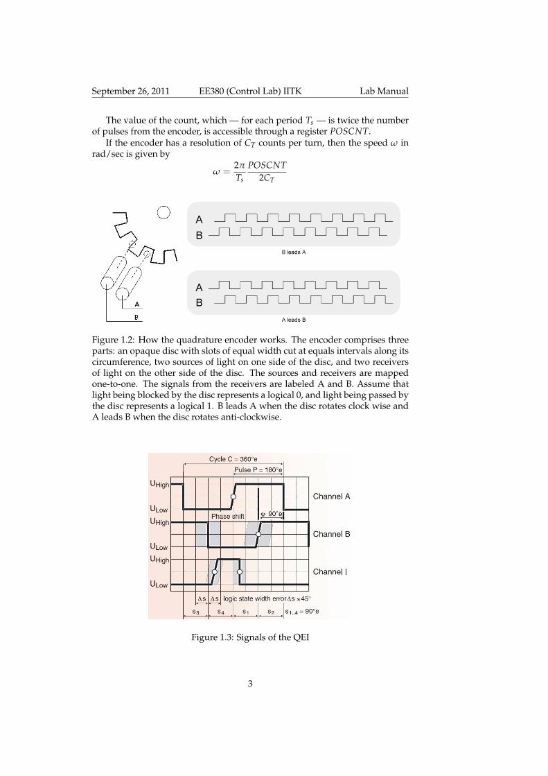
It is used to interface the motor speed encoder to calculate the speed. Figure 1.2explains the working of the quadrature encoder. The signals of the QEI areshown in Figure 1.3. The QEI is configured in x2 mode (QEICON< 10 : 8 > =101). In this mode both edges — rising and falling — of the phase-A signalcause the position counter to change value (increment or decrement). Thephase-B signal is utilized for the determination of the position counter’s di-rection (increment or decrement).
2
September 26, 2011 EE380 (Control Lab) IITK Lab Manual
The value of the count, which — for each period Ts — is twice the numberof pulses from the encoder, is accessible through a register POSCNT.
If the encoder has a resolution of CT counts per turn, then the speed ω inrad/sec is given by
ω =2π
Ts
POSCNT2CT
Figure 1.2: How the quadrature encoder works. The encoder comprises threeparts: an opaque disc with slots of equal width cut at equals intervals along itscircumference, two sources of light on one side of the disc, and two receiversof light on the other side of the disc. The sources and receivers are mappedone-to-one. The signals from the receivers are labeled A and B. Assume thatlight being blocked by the disc represents a logical 0, and light being passed bythe disc represents a logical 1. B leads A when the disc rotates clock wise andA leads B when the disc rotates anti-clockwise.
Figure 1.3: Signals of the QEI
3
September 26, 2011 EE380 (Control Lab) IITK Lab Manual
1.2.4 Universal Asynchronous Receiver Transmitter (UART)Module
This is used to communicate with Personal Computer (PC). We use this to sendthe data of speed and controller output (which is the voltage we wish the H-bridge to apply to the motor) to the PC for plotting. UART is configured withone stop bit and the register U1BRG is used to set the baud rate. Let BR be thebaud rate then the register value is given by
U1BRG =FCY
16BR− 1
In our program, the baud rate is 115200. This is the maximum possible baudrate for our dsPIC board with 29.492 MHz oscillator and its correspondingvalue for the U1BRG register is 0x0003.
1.2.5 GPIO Pins
The GPIO pin D0 is used as a digital output to change the polarity of the volt-age output by the H-bridge (to change the direction of the rotation of the mo-tor). The data direction register (TRISx) determines whether the pin is an input(1) or an output (0). Reading or writing the latch is done by using LATx.
See the section titled pwm_control function in the file setting-prog.h forfurther details.
In our case, TRISD = 0 (Port D is configured as output port).
1.2.6 Analog to Digital Convertor (ADC)
Pins AN(0-2) are configured as analog inputs by using register ADPCFG. Autoconversion mode is used (SSRC(2:0) = 111). The analog input to be convertedis selected using ADCHS register (CH0SA(3:0) bits e.g. 000 for AN0, 001 forAN1). In settings program AN0 is alone selected for conversion.
1.3 Choice of sampling interval
As our microcontroller does not have enough on-chip memory to hold the datawe generate during each control run of the setup, we communicate to the PCthe data as and when it is generated, which means within each sampling in-terval. In the experiments we do in EE380, this data is that of position, speed,armature voltage, and current.
If we wish to communicate only two of these variables to the PC, then itseems that Ts = 0.002 s may be adquate. In our earlier trials, when we triedto communicate three variables to the PC, we found that, while a sampling in-terval of 0.002 s was not adequate, even a sampling interval of 0.003 s, whichseems to be a reasonable choice, was not adequate occassionally. Here, by inad-equate, we mean that the log file created by terminal.exe seemed to containnon-numeric data where it should have contained numeric data. We attributethis inadequacy to the non-realtime nature of how MS Windows may handleUART communication given that we have not made a provision for handshak-ing signals (see Subsection 1.5.1).
4

September 26, 2011 EE380 (Control Lab) IITK Lab Manual
Wait for timer interrupt
Reset the timer interrupt enable flag (IFS0bits.T1IF=0)
Send the speed to UART transmit register
Send the controller output value to UART transmit register
Update the controller action and generate the controller output
Calculate the speed/position using the QEI count register & reset the QEI count
register
Figure 1.4: Flow chart of the ISR in main-prog.c. Interrupt enable flag reset Calculation of speed and reset the QEI count register UART Communication Controller update 0 Timer interrupt Ts 2Ts
PWM Figure 1.5: Timing diagram for the tasks that the ISR implements.
1.4 Characteristics of the H-bridge board
This section is based on tests we performed in preparation for this laboratory.Figure 1.6-left shows that the relationship between the microcontroller out-
put (u) and the H-bridge ouput (Vm) is nonlinear. This relationship is a straightline when the duty ratio is greater than 2/12 (in the figure, u ≈ 2 V corresonds
5

September 26, 2011 EE380 (Control Lab) IITK Lab Manual
0 0.05 0.1 0.150
0.1
0.2
0.3
0.4
Motor current in A
Sen
sed
curr
ent i
n A
-10 -5 0 5 10-10
-5
0
5
10
u in V
Vm
and
Vse
ns in
V
V
m
Vsens
Figure 1.6: Left-fig: The blue curve is the voltage Vm output by the H-bridgeversus the input voltage set by micro-controller (u); the black curve is the volt-age across the sensing resistor (Rs = 5Ω) versus u. The supply voltage is 12V. Right-fig: The current isens through the sensing resistor versus actual motorcurrent i.
to a duty ratio of 2/12 because Vs = 12 V). This relationship has a dead zonewhen the duty ratio is less than 2/12. This characteristic will concern us whenthere is a reversal in the direction of rotation of the motor shaft (for example,in experiments 2 and 3).
Figure 1.6-right shows the relation between the actual motor current (i) andthe current isens sensed using the sensing resistor Rs for Vs =const and TL =var. From this data, we concluded the following approximate relationship:i ≈ 0.533isens − 0.027.
Using isens and the drop VH in the H-bridge, we found that the H-bridgehas a resistance RH of about 27.5 ohm. VH and RH were determined as VH =u−Vm−Vsens and RH = VH/isens. Vm and Vsens were measured using a digitalmultimeter (DMM). Isens was found as isens = Vsens/Rs.
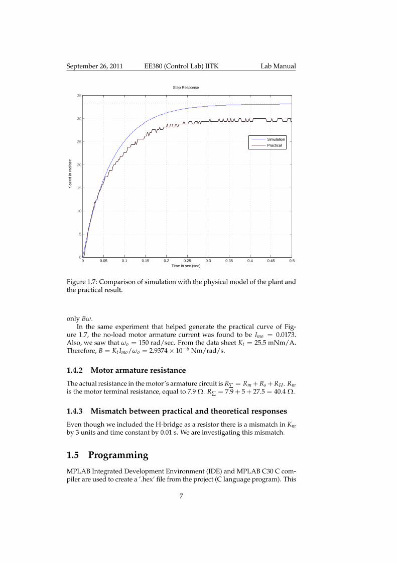
A step signal output by the controller corresponding to a magnitude of 5V causes the motor without load to have a steady state speed of ωo = 150rad/sec. The response is divided by 5 and plotted in Figure 1.7. Also plottedin the same figure is the unit step response of the transfer function (TF) of thesame motor.
The motor’s TF is approximated to first order as in Equation (2.1). Thevalues of the parameters in this TF are all directly or indirectly determinedfrom Table 1.1 and converted into SI units. While KT and J can be read offthe table, and Kb — the back EMF constant — is the reciprocal of the speedconstant, B and R∑ need a little thought.
1.4.1 Calculation of B
Bω is the viscous friction torque in the bearings of the motor, and B is thecoefficient of viscous friction in the bearings. It has been found that the viscousfriction (as opposed to rolling friction, Coulomb friction, etc) is the dominantcomponent of bearing friction.
When no load is applied to the motor shaft (TL = 0) and the speed is steady( dω
dt = 0), the developed torque of the motor Kti needs to be enough to equal
6
September 26, 2011 EE380 (Control Lab) IITK Lab Manual
0 0.05 0.1 0.15 0.2 0.25 0.3 0.35 0.4 0.45 0.50
5
10
15
20
25
30
35
Step Response
Time in sec (sec)
Spe
ed in
rad
/sec
Simulation
Practical
Figure 1.7: Comparison of simulation with the physical model of the plant andthe practical result.
only Bω.In the same experiment that helped generate the practical curve of Fig-
ure 1.7, the no-load motor armature current was found to be Imo = 0.0173.Also, we saw that ωo = 150 rad/sec. From the data sheet Kt = 25.5 mNm/A.Therefore, B = Kt Imo/ωo = 2.9374× 10⁻⁶ Nm/rad/s.
1.4.2 Motor armature resistance
The actual resistance in the motor’s armature circuit is R∑ = Rm +Rs +RH . Rmis the motor terminal resistance, equal to 7.9 Ω. R∑ = 7.9 + 5 + 27.5 = 40.4 Ω.
1.4.3 Mismatch between practical and theoretical responses
Even though we included the H-bridge as a resistor there is a mismatch in Kmby 3 units and time constant by 0.01 s. We are investigating this mismatch.
1.5 Programming
MPLAB Integrated Development Environment (IDE) and MPLAB C30 C com-piler are used to create a ’.hex’ file from the project (C language program). This
7

September 26, 2011 EE380 (Control Lab) IITK Lab Manual
’.hex’ file will be loaded to the dsPIC30F4012 through PICKIT-2 using PICKIT2v2.61 software. We wrote a code to configure all the modules that are neces-sary for our setup. In that code the controller part alone needs to be modifiedaccording to your own designed controller. The simple procedure to write aprogram into dsPIC is as follows:
• Run the MPLAB IDE and open the project file which we have provided youon the Desktop of your PC.
• In that project C-program file the controller code part should be modified toform your own designed controller.
• Save all and go to Project→ Build All. Make sure that the PICkit 2 is chosenin Programmer→ Select Programmer.
• Export the .hex file (File → Export) and remember the file name and loca-tion.
• Run the PICkit 2 Programmer software, choose the device family dsPIC30,import the ’.hex’ file, and write the program to dsPIC30F4012 by pressingthe Write command button.
1.5.1 Reading the data from dsPIC to PC
Run the Hyper Terminal or Terminal.exe (from the Desktop), choose COM1Port, set Baud rate to 115200, 8-data bits, none parity bit, 1-stop bit and nonehandshaking bit. Store the data in the text file and import the data to MATLAB.The odd indexed data are values of speed (ω(i ∗ Ts) = datai; i = 1, 3, 5, · · · )in rad/sec. The even indexed data are 100 times the controller output data(v(i ∗ Ts) = datai/100; i = 2, 4, 6, · · · ) in volts.
1.6 Parameters of DC motor-gear-encoder unit
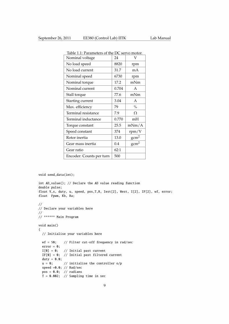
The parameters of our DC motor are reproduced from Maxon Motors’ catalogin Table 1.1. For data sheets of the motor, gear, and encoder, Google with thefollowing key words: A-max26 110963 (for motor), GP26B 144036 (for gear),and HEDS 5540 110511 (for encoder). These three items are from Maxon Motor(www.maxonmotor.com).
1.7 Program listings
1.7.1 main-prog.c// main-prog.c.
#include<p30f4012.h>#include "settings-prog.h"_FOSC(CSW_FSCM_OFF & XT); // To use the external crystal_FWDT(WDT_OFF); // To disable the watchdog timer
// split the data by decimal digits (0 - 9) in 3 digit form
8
September 26, 2011 EE380 (Control Lab) IITK Lab Manual
Table 1.1: Parameters of the DC servo motor.Nominal voltage 24 V
No load speed 8820 rpm
No load current 31.7 mA
Nominal speed 6730 rpm
Nominal torque 17.2 mNm
Nominal current 0.704 A
Stall torque 77.6 mNm
Starting current 3.04 A
Max. efficiency 79 %
Terminal resistance 7.9 Ω
Terminal inductance 0.770 mH
Torque constant 25.5 mNm/A
Speed constant 374 rpm/V
Rotor inertia 13.0 gcm2
Gear mass inertia 0.4 gcm2
Gear ratio 62:1
Encoder: Counts per turn 500
void send_data(int);
int AD_value(); // Declare the AD value reading functiondouble pulse;float V_s, duty, u, speed, pos,T,R, Iest[2], West, I[2], IF[2], wf, error;float Fpwm, Kb, Ra;
//// Declare your variables here//// ****** Main Program
void main()// Initialise your variables here
wf = 50; // Filter cut-off frequency in rad/secerror = 0;I[0] = 0; // Initial past currentIF[0] = 0; // Initial past filtered currentduty = 0.0;u = 0; // initialise the controller o/pspeed =0.0; // Rad/secpos = 0.0; // radiansT = 0.002; // Sampling time in sec
9
September 26, 2011 EE380 (Control Lab) IITK Lab Manual
Fpwm = 50; // PWM Frequency in kHzV_s = 12.0; // Power supply VoltageTRISD = 0; // D port is configured as output portLATD = 1; // used for direction controlqei_set(); // Initialise QEI settingspwm_set(Fpwm); // Initialise PWM settingsuart_set(); // Initialise UART settingsAD_set(); //Initialise ADC settingstimer1_set(T); // Initialise Timer-1 settings and starts the timerTRISEbits.TRISE8 = 0; // RE8 is configured as output
// Continue until stop the powerfor(;;);
// End of main()
// Interrupt service routine (ISR) for interrupt from Timer1
void __attribute__((interrupt, no_auto_psv)) _T1Interrupt (void)IFS0bits.T1IF = 0; // Clear timer 1 interrupt flag
// To calculate the execution time of the controller code make E8 = 1
LATEbits.LATE8 = 1;uart_tx(9);
// QEI count feedback// if motor is in anticlockwise direction,count goes down from FFFF.
if(POSCNT > 0x8000)pulse = 0xFFFF - POSCNT;pulse = - pulse;
elsepulse = POSCNT;
POSCNT = 0; // Reset the QEI count
// Calculation of speed (rad/s)// speed = 2*pi*( no of pulse/(2*500) )/T in (rad/sec)speed = 6.2831853 * pulse/1000/T;send_data(speed); // Transmit the speed
// Calculation of position (rad)// pos_current = pos_past + 2*pi*( no of pulse/(2*500) )/Rg in (rad)// Rg = 62 gear ratio// pos = pos + 6.2831853 * pulse/62000;// send_data(pos*100); // Transmit the position *100
// In the experiment where we input a sine wave that lies in the// interval [0,5] V, and the speed reference is a sinusoid, enable// the following two lines to give the reference input.// R = AD_value(); // In signed mode, ADC maps [0,5] V to [-511,+511].// R = 150*R/511; // R = 150*sin(w_in*t) rad/sec; 150 is max speed.
10

September 26, 2011 EE380 (Control Lab) IITK Lab Manual
// Uncomment following lines in experiments where current feedback used./*IV = AD_value(); // Read voltage across Rs=4.7ohm.IV = 5*(511 + IV)/1022; // Convert signed to unsigned.I[1] = IV/4.7; // Convert voltage to current.
// Low-pass filter with cut-off frequency wf:IF[1] = (wf*T/(2+wf*T))*(I[1]+I[0])+((2-wf*T)/(2+wf*T))*IF[0];// Prepare IF[0] and I[0] for the next sampling intervalIF[0] = IF[1];I[0] = I[1];
*/
// Only if you want to observe filtered current, uncomment following line//// send_data(IF[1]*1000);//// Why the 1000? We have observed in our trials that the current is// less than 1 A in magnitude. Irrespective of what the actual values// may be, for convenience, we send integers of at most 3 digits from// the UART module. Therefore, when the current is upto 0.999 in// magnitude, we multiply its value by 1000. If we find that it exceeds// 0.999, then we may choose to multiply by a number that will result// in a product of at most 999.
/*************************************//**** Your controller code *****//***** goes in place of this box *****//*************************************/
// u=7; // For step input uncomment this to provide step of 7
if(u > 0.8 * V_s)u = 0.8 * V_s; // Positive saturation
else if(u < -0.8 * V_s)u = -0.8 * V_s; // Negative saturation
duty = u/V_s;pwm_con(duty); // Update the PWM with respect ot the new duty ratiouart_tx(9);send_data(u*100); // Sending 100 times control effort u.
LATEbits.LATE8=0; // End of ISR of Timer 1
void send_data(int s_data)int s;if(s_data < 0)// Send the negative sign (ASCII is 45)uart_tx(45);
11

September 26, 2011 EE380 (Control Lab) IITK Lab Manual
s_data = -1*s_data;
// Digit with the position value of 100s = s_data/100;uart_tx(s+48);
// Digit with the position value of 10s_data = s_data - (s *100);s = s_data/10;uart_tx(s+48);
// Digit with the position value of 1s_data = s_data - (s *10);uart_tx(s_data+48);
// End of send_data()
int AD_value()int count, *ADC16Ptr, ADCValue = 0; // clear valueADC16Ptr = &ADCBUF0; // Initialize ADCBUF pointerADCON1bits.ADON = 1; // Turn ADC ONIFS0bits.ADIF = 0; // Clear ADC interrupt flagADCON1bits.ASAM = 1; // Auto start sampling
while (!IFS0bits.ADIF); // Conversion done?ADCON1bits.ASAM = 0; // If YES then stop sample/convertfor (count = 0; count < 2; count++) // Average the 2 ADC valueADCValue = ADCValue + *ADC16Ptr++;
ADCValue = ADCValue >> 1; // ‘‘>>’’ represents ‘‘shift by 1 to left’’.// Equivalent to ‘‘divide by 2’’.
return(ADCValue);// End of AD_value()
1.7.2 settings-prog.h// Settings prog for the board with 29.492MHz crystal osc// ********* UART settings//________________________
/* Notes: Fcy = Fosc/4 = 29492000/4 = 7373000HzU1BRG = Fcy/(16 * Baud_Rate) - 1conf: 1 stop bit, 8 data bit, no parity*/
#include<p30f4012.h>
void timer1_set(float); // Timer-1 settingsvoid qei_set(); // QEI settingsvoid pwm_set(int); // PWM settingsvoid pwm_con(float); // PWM control based on duty ratiovoid uart_tx(int); // UART data to be transfered to PC
12

September 26, 2011 EE380 (Control Lab) IITK Lab Manual
void uart_set(); // UART settingsvoid AD_set(); // A-D settings
// ******* pwm_control functionvoid pwm_con(float Duty) int pdc;pdc = Duty * 2 *(PTPER + 1);if(pdc == 0)LATDbits.LATD0 = 1;else if(pdc < 0)LATDbits.LATD0 = 0; // RD0 = 0pdc = 2*( PTPER+1) + pdc;else if(pdc > 0)LATDbits.LATD0 = 1; // RD0 = 1PDC1 = pdc;// ******* End of pwm_control function//------------------------------------------------------------//// ******* Timer-1 settingsvoid timer1_set(float Ts)IEC0bits.T1IE = 1; // Enable Timer-1 interruptIFS0bits.T1IF = 0; // Clear Timer-1 interrupt flag to get next interruptPR1 = 7373000*Ts; // No of clk (count) per controller sampling timeTMR1 = 0; // Initialise the Timer countT1CON = 0x8000; // Starts the timer, Internal clock (Fosc/4), prescale 1:1// ******* End of Timer-1 settings//------------------------------------------------------------//// ******* QEI module settingsvoid qei_set()ADPCFG = 0x0038; // Config all the AN(3-5)/RB(3-5) pins are in Digital I/O mode// AN(0-2) pins are in Analog modeIEC2bits.QEIIE = 0; // Disable interrupt due to QEIIFS2bits.QEIIF = 0; // Clear the interrupt flagQEICON = 0; // Default mode: QEI mode/timer offQEICONbits.QEIM= 5;DFLTCON = 0x0100; // No filter operationPOSCNT = 0; // Initialize position of counterMAXCNT = 0xFFFF; // set maxcount limit// ******* End of QEI module settings//------------------------------------------------------------//// ******* PWM module settingsvoid pwm_set(int F_pwm) // PWM timer was enabled, 1:1 prescale Tcy, 1:1 Postscale,PTCON = 0x8000; // PWM time base operates in a free running mode
13

September 26, 2011 EE380 (Control Lab) IITK Lab Manual
PTPER = 7373/F_pwm - 1; // PWM Time Base Period Register (Period of PWM)// Note: PTPER = Fcy/(Fpwm*PTMER_prescaler) - 1
// Fcy =Fosc/4 = 7373000PWMCON1 = 0x0011; // PWM I/O pin pair is in the complementary output mode// PWM1L and PWM1H are enabled remainings are in I/O modePDC1 = 0; // Initaily Duty ratio is zero;OVDCON = 0x0303; // Controlled by PWM modulePTMR = 0x0000; // PWM Time Base Register initialized// ******* End of PWM settings//------------------------------------------------------------//
// ******* Transmit the Data through UARTvoid uart_tx(int tx_data)while(U1STAbits.UTXBF == 1)// wait to the UART transmit buffer gets one emty space// if(U1STAbits.UTXBF!=1) // If the buffer is not full transmit the data
U1TXREG=tx_data; // Transmit// ******* End Transmit the Data through UART//------------------------------------------------------------//
void uart_set()U1MODE = 0x8400; // 1-stop bit and U1ARX, U1ATX are used//U1MODE = 0x8000; // 1-stop bit and U1RX, U1TX are usedU1STAbits.UTXEN = 1; // Enable the UART transmiterU1STAbits.UTXISEL = 0; // Interrupt generated when any character is
//transferred to the transmit registerIEC0bits.U1TXIE = 1; // Enable the Interrupt for the TransmiterIFS0bits.U1TXIF = 0; // Clear the transmiter Interrupt flag to transmitIEC0bits.U1RXIE = 1; // Enable the Interrupt for the ReceiverIFS0bits.U1RXIF = 0; // Clear the transmiter Interrupt flag to receiveU1BRG = 0x0003; // Baud_rate 115200//U1BRG = 0x0007; // Baud_rate 57600
// ***** UART Transmit ISRvoid __attribute__((interrupt, no_auto_psv)) _U1TXInterrupt(void)IFS0bits.U1TXIF = 0; // clear TX interrupt flag
// ***** UART Receive ISRvoid __attribute__((interrupt, no_auto_psv)) _U1RXInterrupt(void)IFS0bits.U1RXIF = 0; //clear receive interrupt flag/* while (U1STAbits.URXDA)speedset=U1RXREG;
14
September 26, 2011 EE380 (Control Lab) IITK Lab Manual
// */if(U1STAbits.OERR == 1)U1STAbits.OERR = 0; // Clear Overrun Error to receive data
//------------------------------------------------------------//
// ***** A to D (A/D) Settingsvoid AD_set()ADPCFG = 0x0038; // Config all the AN(3-5)/RB(3-5) pins are in Digital I/O mode// AN(0-2) pins are in Analog mode
ADCON1 = 0x01E0; // SSRC bit = 111 (auto convert) implies internal// counter ends sampling and starts converting.ADCHS = 0x0000; // Connect RB0/AN0 as CH0 input.ADCSSL = 0;ADCON3 = 0x0F00; // Sample time = 15Tad, Tad = internal Tcy/2ADCON2 = 0x0004; // Interrupt after every 2 samples
1.7.3 readplot.m
% readplot.m: Uses GNU Octave’s or MATLAB’s dlmread% function to read the contents of the file% testdata.txt into a vector. This file belongs to the% lab manual for EE380 (control lab).%% The file testdata.txt is generated as follows. The% program terminal.exe writes the information that it% receives from dsPIC30F4012 to the file testdata.txt.% The program in dsPIC30F4012 sends this information% as tab seperated ASCII values.%% We have tested that this m-file executes nicely in% GNU Octave version 3.2.4 that comes packaged for Windows in%% http://sourceforge.net/projects/octave/files/% Octave_Windows%20-%20MinGW/% Octave%203.2.4%20for%20Windows%20MinGW32%20Installer/% Octave-3.2.4_i686-pc-mingw32_gcc-4.4.0_setup.exe/download%% and MATLAB 7.7.0471 (R2008b) that we have in our CC.% On MATLAB dlmread(’testdata.txt’) seems to be returning% the last item in the vector as 0 even though it may be% blank. GNU Octave does not have this problem.%% The plots are generated nicely in MATLAB and the Linux
15
September 26, 2011 EE380 (Control Lab) IITK Lab Manual
% version of GNU Octave. The plotting program (most likely% GNUPlot) in the windows version of GNU Octave does not% seem to be properly integrated into GNU Octave. So, we% have trouble displaying the results of plot on the screen.% As a work around, we have used the command%% print -djpg plot.jpg%% to print the plots to jpeg files.%% We found that this problem has been reported at%% http://octave.1599824.n4.nabble.com/% Gnuplot-freezes-in-Win7-3-2-4-td2279218.html#a2279218%% and a work-around has been suggested there and at%% http://old.nabble.com/% Re:-Octave-3.2.4-mingw32-available-p28053703.html%% Using this work-around does remove this problem.%% readplot.m can replace plot-prog.m that we have been% using thus far.%% PRECONDITIONS: readplot.m and testdata.txt need% to be in the same folder. All data in testdata.txt is% tab-separated and in a single row.%% Date created on: September 12, 2010.%%%%%%%%%%%%%%%%%%%%%%%%%%%%%%%%%%%%%%%%%%%%%%%%%%%%%%%%%
clear all, close all, clc
x = dlmread(’testdata.txt’);
% Determine the number of rows and columns of x.% If all went well, the number of rows will be equal to 1.[rows,cols] = size(x);
% Truncate x so that x has an even number of columns.if cols/2 > floor(cols/2)x = x(:,1:cols-1);cols = cols-1;
end
% Extract columns number 1, 3, 5, ... into a vector w,% and columns number 2, 4, 6, ... into a vector u.w = x(1,1:2:cols-1); % This is the vector of speedsu = x(1,2:2:cols); % This is the vector of voltages.
16

September 26, 2011 EE380 (Control Lab) IITK Lab Manual
% Calculate times at which to plot speed and voltage.T = 0.002; % sampling timet = 0:T:T*(cols/2-1);
% Plot the speeds and the voltages with respect to time.subplot(2,1,1); plot(t,w); grid;title(’Speed of the motor shaft in (rad/s)’);subplot(2,1,2); plot(t,u); grid;title(’Voltage applied to motor in (V)’);
print -djpg plots.jpg
17


September 26, 2011 EE380 (Control Lab) IITK Lab Manual
1.8 Schematic of the dsPIC30F4012 board
11
22
33
44
DD
CC
BB
AA
Titl
e
Nu
mbe
rR
evis
ion
Siz
e
Lett
er
Dat
e:7/
27/2
010
She
et
of
File
:C
:\D
ocu
men
ts a
nd S
ettin
gs\..
\PIC
-boa
rd.S
chD
ocD
raw
n B
y:
MC
LR1
EMU
D3
/AN
0/V
RE
F+
/CN
2/R
B0
2
EM
UC
3/A
N1
/VR
EF-
/CN
3/R
B1
3
AN
2/S
S1/C
N4/
RB2
4
AN
3/IN
DX
/CN
5/R
B35
AN
4/Q
EA/IC
7/C
N6
/RB
46
AN
5/Q
EB
/IC
8/C
N7
/RB
57
VSS
8
OS
C1
/CL
KI
9
OSC
2/C
LKO
/RC
151
0
EM
UD
1/S
OS
CI/
T2C
K/U
1AT
X/C
N1/
RC
131
1
EMU
C1/
SOSC
O/T
1CK
/U1A
RX
/CN
0/R
C1
41
2
VD
D1
3
EM
UD
2/O
C2/
IC2/
INT
2/R
D1
14
EMU
C2/
OC
1/IC
1/IN
T1
/RD
01
5
FLT
A/I
NT
0/S
CK
1/O
CF
A/R
E8
16
PG
D/E
MU
D/U
1T
X/S
DO
1/S
CL
/C1
TX
/RF
31
7P
GC
/EM
UC
/U1
RX
/SD
I1/S
DA
/C1R
X/R
F2
18
VSS
19
VD
D2
0
PWM
3H
/RE
52
1P
WM
3L
/RE
42
2PW
M2
H/R
E3
23
PW
M2
L/R
E2
24
PWM
1H
/RE
12
5P
WM
1L
/RE
02
6
AV
SS2
7
AV
DD
28
U2
dsP
IC3
0F40
12-3
0I/
SP
VC
C
MR
1
VC
C2
GN
D3
PF
I4
PF
O5
WD
I6
RS
T7
WD
O8
U1-
MA
X70
6P
CP
A
D1
1N
414
8
VC
C
S1 PB
IN1
3
OU
T2
GN
D
VR
L78
05C
V
.22u
FC
1.1
uF
C2
VC
C+1
2V
-12V
+1
2V
27p
F
C3
Cap
27p
F C4
Cap
1 2
Y1
29.4
92 M
Hz
OS
C1
OS
C1
1 2 3 4 5 6
CN
2-PI
CK
IT2
MC
LR
MC
LR
PW
M1L
PW
M1H
RE
2R
E3
RE
4R
E5
TX
D1
VS
S2
VD
D3
RX
D4
VR
EF
5
CA
NL
6
CA
NH
7
RS
8
U3
MC
P2
551-
I/P
1KR2
1KR3
VC
C
120
E
R4
Res
1
CA
N1
CA
N2
DS
1
LE
D1
470
ER
1
OS
C2
OS
C2
RD
01 2 3
JP8
RE
8
RE8
RE
8-I
U1
AT
XU
1A
RX
RD
1
1 2 3 4 56 7 8 9
11 10
DB
9-C
AN
DB
9
CA
N1
CA
N2
1 2 3
JP9
QE
VC
C
NE
T
RB
0R
B1
RB
2
QE
B-I
QE
A-I
QE
I-I
1 2 3
CN
1-P
S
E8-
O
1 2 3
JP4 1 2 3
JP5 1 2 3
JP6 1 2 3
JP7
1 2 3
JP31 2 3
JP1 1 2 3
JP2
RB
0
RB
1
RB
2
RE2
RE5
RE3
RE4
B0-
O
RB
0-I
B1-
O
RB
1-I
RB
2-I
B2-
O
RE
2-I
E2-
O
RE
3-I
E3-
O
RE
4-I
E4-
O
RE
5-I
E5-
O
C1R
XC
1TX
C1R
XC
1TX
C1R
X
C1T
X
2 31
4 111
U4
ALF
347
BN
4 11
567
2
U4
BL
F3
47B
N
4 11
8109
3
U4C
LF
347
BN
4 11
14
1213
4
U4
DL
F347
BN
PW
M1L
PWM
1H
RD
OR
D1
+12V
-12
V
2 31
4 111
U5A
LF
347
BN
4 11
567
2
U5
BL
F3
47B
N
4 11
81
09
3
U5
CL
F3
47B
N
4 11
141213
4
U5
DL
F3
47B
NQ
EA
QE
BQ
EI
+12V
-12
V
PW
M1
L-O
PW
M1
H-O
SD
1SD
2
QE
B-I
10K
R8
3.3
K
R9
3.3
K
R10
Res
13
.3K
R11
Res
11
0KR
12
10K
R7
10K
R6
10K
R5
NE
TN
ET
NE
T
2 31
4 111
U6A
LF
347
BN
4 11
567
2
U6
BL
F3
47B
N
4 11
81
09
3
U6
CL
F3
47B
N
4 11
141213
4
U6
DL
F3
47B
N
+12V
-12
V
10K
R13
10K
R14
10K
R15
10K
R16
2 31
4 111
U7A
LF
347
BN
4 11
567
2
U7
BL
F3
47B
N
4 11
81
09
3
U7
CL
F3
47B
N
4 11
141213
4
U7
DL
F3
47B
N
+12V
-12
V
10K
R17
10K
R18
10K
R19
10K
R20
RE8
-O
B0-
OB
1-O
B2-
OE2
-O
QE
I-I
E3-
OE
4-O
E5
-OE8
-O
RB
0-O
RB
1-O
RB
2-O
RE
2-O
RE
8-O
RE
5-O
RE
4-O
RE
3-O
QE
A-I
12
34
56
78
91
0
CN
3-M
OT
OR
12
34
56
78
91
0
CN
4-I
/P
12
34
56
78
91
0
CN
5-O
/P
VC
C
PW
M1L
-OP
WM
1H-O
SD
1S
D2
QE
AQ
EB
QE
I
RB
0-I
RB
1-I
RB
2-I
RE
2-I
RE
3-I
RE
4-I
RE
5-I
RE
8-I
RB
0-O
RB
2-O
RB
1-O
RE3
-OR
E2
-OR
E4
-OR
E8
-OR
E5-O
1 2 3
CN
6-U
ART
Hea
der
3
U1
-PC
-TX
U1
-PC
-RX
4
12
19
3 20
5 18
C1+
8C
2+1
1
GN
D6
C1-
13
VC
C7
R1
T1
T2 R
2
C2-
16
V-
12
V+
14
GN
D9
C2+
15
C2-
10
V-
17
U8
-MA
X2
33A
MA
X23
3AC
PP
VC
C1
uFC
5
U1
AT
X
U1A
RX
U1
A-P
C-T
X
U1
A-P
C-R
X
1 2 3 4 56 7 8 9
11
10
DB
9-U
AR
T-A
C1R
X
C1T
X
U1
-PC
-TX
U1
-PC
-RX
1 2
JP9-
U1
TX
1 2
JP10
-U1R
X
U1
TX
U1
TX
U1
RX
U1
RX
dsP
IC30
F401
2 bo
ard
19

September 26, 2011 EE380 (Control Lab) IITK Lab Manual
20

Chapter 2
Experiment 1: PMDC motormodeling, identification,speed control
2.1 Goals
For a PMDC motor develop a physics-based model and a model-based onexperimentation using open-loop (OL) step response. Design & implementa speed controller for each model using Bode plot-based loop-shaping tech-niques. Compare the results.
2.2 Introduction
The block diagram of the setup is as shown in Figure 1.1.Section 2.3 lists the steps through which we wish to achieve the above-
stated goals. Sections 2.4 onwards fill in the technical background needed toexecute these steps.
2.3 Exercises
2.3.1 To do at home
Q1 Determine the physics-based mathematical model of the DC servo motorwhose parameters are given in Table 1.1. See Section 2.4.
Q2 Design using Bode plot-based loop-shaping techniques a controller of theminimum order possible to control the speed of the given motor for the fol-lowing time domain specifications: ess ≤ 2%, ts ≈ 0.5 s (you have upto 5%tolerance on ts), Mp ≤ 20%.
A 5-cycle semilog graph paper is provided at the end of this chapter.
Q3 Simulate the continuous-time controller designed above using GNU Oc-tave.
21
September 26, 2011 EE380 (Control Lab) IITK Lab Manual
If the closed-loop system performance in simulation is not as desired, youmay need to redesign your controller.
Q4 Discretize the continuous-time controller with the sampling period Ts.
Q5 With the discretized version, perform a simulation of digital control of thecontinuous-time plant using the m-file provided.
Do you think that your digitally-controlled closed-loop system will be stablein practice? Will it provide in practice the same performance as did thecontinous-time version in simulation?
Q6 Write the digital controller in C.
2.3.2 To do in lab
Q7 Write a code to give a step voltage input to the given motor. Run the setupin OL mode.
Q8 Identify the system parameters Km and τm by using the OL step response.
Q9 For the identified model, redesign your controller using loop-shaping onthe graph paper provided.
Q10 With the discretized version of the above-redesigned controller, performa simulation of digital control of the continuous-time plant using the m-fileeasysim.m.
Q11 Program the lab-designed digital controller and run the setup.
Q12 Perform the following comparisons.
1. The performance of the controller designed for the physics-based modelin simulation and in experiment.
2. The performance of the controller designed for the identified model insimulation and in experiment.
Q13 Conclusions:
1. Is the physics-based model a good match to the plant? If not, what doyou think we have ignored that has lead to the difference?
2. To what extent did you learn through this experiment each of the skillslisted in Section 2.2?
3. Would you have preferred to learn a different skill set from the controllab? If yes, which skills?
4. How could we have organized this experiment differently to make itmore meaningful to you?
2.4 Physics-based model of the DC motor unit
Since the inductance La is very small1, by neglecting La, from Figure 2.1, thetransfer function (TF) from the input voltage V(t) to the speed ω(t) of the mo-
1When is an inductor considered small? When the time constant due to this inductor is neg-ligible in comparison to the remaining time constants in the TF of the system, this inductor isconsidered neglibly small.
22

September 26, 2011 EE380 (Control Lab) IITK Lab Manual
V(s) + 1sLa + RΣ
KtI(s) T(s) +
TL(s)− 1
Js + B
ω(s)
Kb
−
Figure 2.1: Block diagram of a PMDC motor. RΣ includes the armature resis-tance Ra and other resistances as explained in Subsection 1.4.2.
tor shaft isω(s)V(s)
=Km
τms + 1(2.1)
with
Km =KT
R∑B + KTKb, (2.2)
τm =R∑ J
R∑B + KTKb(2.3)
Here, Km is the motor gain constant in rad/s/V, τm is the motor time constantin seconds, KT is the torque constant in Nm/A, R∑ is the resistance in thearmature path in ohms as explained in Subsection 1.4.2, B is the viscous-frictioncoefficient of the motor rotor with attached mechanical load in Nm/(rad/sec),J is the moment of inertia of the motor rotor with attached mechanical loadkg-m2, Kb is the back emf constant in V/(rad/sec).
2.5 System identification
As we know that the motor transfer function is theoretically of first order asin Equation (2.1), we can identify Km and τm from the V-to-ω step response asfollows:
Step 1 Apply a step input of magnitude R volts from the microcontroller tothe motor.
This is achieved by generating a number r within the microcontroller that isproportional to R volts. The microcontroller converts r into a suitable dutyratio that is then applied to the H-bridge. The H-bridge will then on theaverage within each sampling interval apply a DC voltage of R volts to themotor.
Step 2 Plot the data of motor speed versus time. This data comes from theencoder to the microcontroller that, in turn, sends to the PC via UART. SeeSubsection 1.5.1.
Step 3 If the armature voltage-to-speed TF is indeed first order, and of the formK/(τs + 1), then the speed will be the following function of time:
ω(t) = RK(1− e−t/τ) (2.4)
Therefore, τ and K can be obtained from the plot of ω versus t as
23
September 26, 2011 EE380 (Control Lab) IITK Lab Manual
• τ is the time where the speed is 0.6321ω(∞)
• RK = ω(∞).
To check that the response is indeed first order, we can plot ω generated byEquation (2.4) on the plot of Step 2, and see how closely the two plots match.If necessary, we may also tweak τ and K so that the two plots match as best aspossible.
2.6 Discretized version of the controller
The controller we design will be in the form of a TF. To program this controllerequation in the microcontroller, we need to recognize that the microcontrollercontrols the motor by sampling the motor states periodically with a samplingperiod of Ts seconds, and that this sampling period may affect the form of thecontroller equation in the microcontroller.
In particular, we “discretize” the controller equation. That is, we convertthe equation from continuous-time form to a discrete-time form. We per-form this discretization through the following steps: convert the controllerinto a state-space equation, discretize this state-space equation, and use thisdiscretized equation for a time-domain recursion. We saw this technique inLecture 30 of EE250-2011. Here we recap this technique.
2.6.1 Conversion from transfer function to state-space
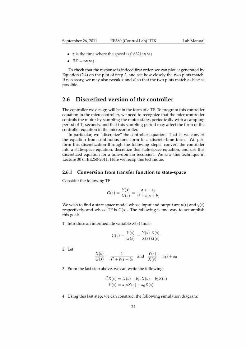
Consider the following TF
G(s) =Y(s)U(s)
=a1s + a0
s2 + b1s + b0
We wish to find a state space model whose input and output are u(t) and y(t)respectively, and whose TF is G(s). The following is one way to accomplishthis goal:
1. Introduce an intermediate variable X(s) thus:
G(s) =Y(s)U(s)
=Y(s)X(s)
X(s)U(s)
2. LetX(s)U(s)
=1
s2 + b1s + b0and
Y(s)X(s)
= a1s + a0
3. From the last step above, we can write the following:
s2X(s) = U(s)− b1sX(s)− b0X(s)Y(s) = a1sX(s) + a0X(s)
4. Using this last step, we can construct the following simulation diagram:
24
September 26, 2011 EE380 (Control Lab) IITK Lab Manual
a01s
1s
b1
b0
U(s)+− −
a1
+
+Y(s)X(s)sX(s)s2X(s)
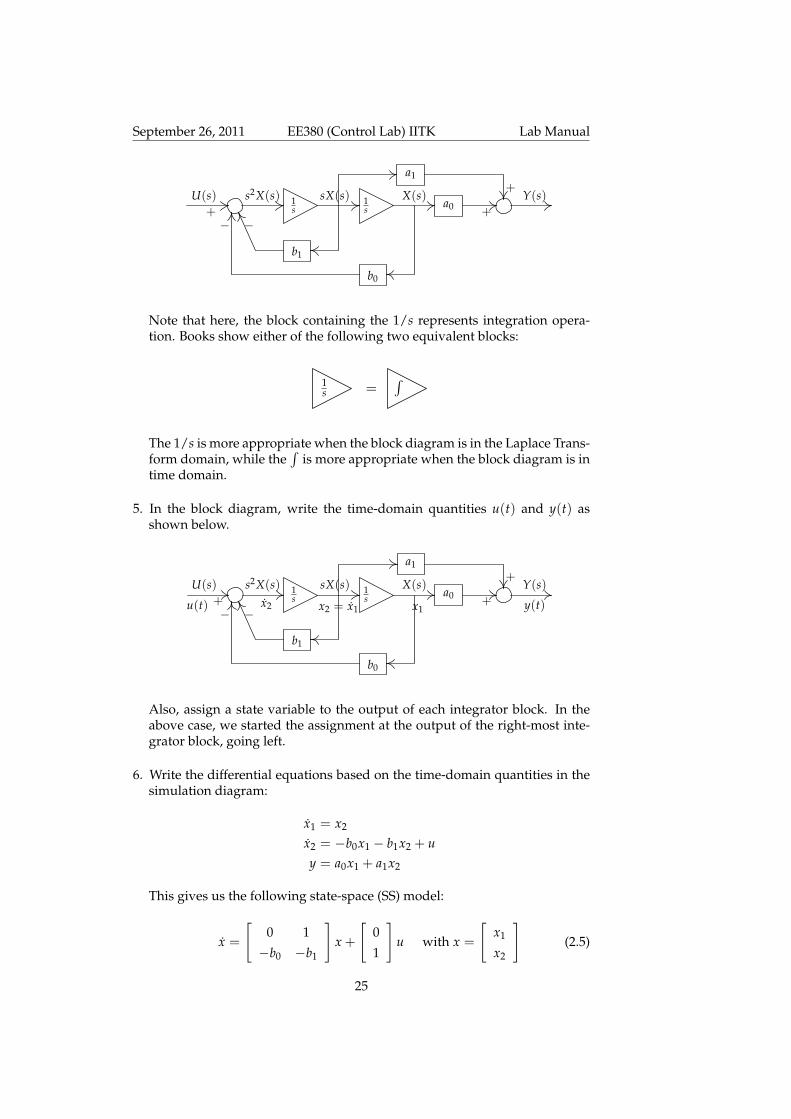
Note that here, the block containing the 1/s represents integration opera-tion. Books show either of the following two equivalent blocks:
1s
∫=
The 1/s is more appropriate when the block diagram is in the Laplace Trans-form domain, while the
∫is more appropriate when the block diagram is in
time domain.
5. In the block diagram, write the time-domain quantities u(t) and y(t) asshown below.
a01s
1s
b1
b0
U(s)+− −
a1
+
+Y(s)X(s)sX(s)s2X(s)
x1x2 = x1x2 y(t)u(t)
Also, assign a state variable to the output of each integrator block. In theabove case, we started the assignment at the output of the right-most inte-grator block, going left.
6. Write the differential equations based on the time-domain quantities in thesimulation diagram:
x1 = x2
x2 = −b0x1 − b1x2 + uy = a0x1 + a1x2
This gives us the following state-space (SS) model:
x =
[0 1
−b0 −b1
]x +
[0
1
]u with x =
[x1
x2
](2.5)
25

September 26, 2011 EE380 (Control Lab) IITK Lab Manual
TIME = kTsfor some integer
START
runcomplete?
Y
Y
Simulation ofcontinuous-timeplant dynamics
N
N
STOP
k?
Update controlu(t) = uk
Figure 2.2: Scheme for simulation of digital control of continuous-time system,adapted from [1]. The control input u(t) is updated at each time kTs, and thenheld until time (k + 1)Ts.
2.6.2 Discretization of the state-space equation
Given the state-space equation x = Ax + Bu, use Euler’s approximation towrite x as x ≈ x(t+∆t)−x(t)
∆t . Then, write this state-space equation as x(t+∆t) ≈(A∆t + I)x(t) + B∆tu(t). This approximation works well if ∆t is sufficientlysmall. As a rule of thumb, ∆t should be at most one-tenth or one-twentieth ofthe smallest eigenvalue of A.
2.6.3 Time-domain recursion
The equation x(t+∆t) ≈ (A∆t+ I)x(t) + B∆tu(t) gives the following formulafor recursion:
x(k + 1) = (ATs + I)x(k) + BTsu(k)
Here, Ts = ∆t.For example, Equation (2.5), on discretization, has the following form that
is ready for recursion:
x1(k + 1) = x1(k) + Tsx2(k)x2(k + 1) = −b0Tsx1(k) + (1− b1Ts)x2(k) + Tsu(k)
In our simulations, we may use Ts = 0.002 s.
2.7 Simulation
The discrete-time controller will work in practice on a continuous-time plant.Let us test this behavior in simulation. The simulation scheme is shown inFigure 2.2 and is implemented in the m-file easysim.m. easysim.m runs on thebase MATLAB and also on GNU Octave.
26
September 26, 2011 EE380 (Control Lab) IITK Lab Manual
2.8 Program listings
2.8.1 easysim.m
% easysim.m: Simulates digital control of continuous-% time system without using MATLAB’s Control System% Toolbox. Uses only Euler’s approximation.%% PRECONDITIONS: (1) User needs to convert plant and% controller TFs to SS. (2) Tp < Ts/10; Ts < Tmin/10.% Here, Tmin is the smallest time constant of the CL system,% Tp is the step size of numerical integration of the plant% dynamics, and Ts is the step size of the numerical% integration of the closed-loop system dynamics. Ts is the% same as the chosen sampling interval.%-------------------------------------------------------------
clc; clear all; close all;
% ------------ Begin declarations ----------------------------
% Plant transfer function K/(s+w)K = 100; w = 1;% State space model of plant is%% xpdot = -w*xp + up;% yp = K*xp;%% The suffix ‘‘p’’ represents plant.
% Controller will sample plant states every Ts secondsTs = 0.01;% We will control the plant for tsfin secondstsfin = 5;
% Step size Tp used for numerical integration of plant% differential equation using Euler’s approximation.Tp = 0.00001;% We will numerically integrate plant differential% equation for Ts seconds.
% Controller TF is Cs = (Kp*s+Ki)/sKp = 0.11;Ki = 1.737;% State-space model of controller is%% xcdot = uc;% yc = Ki*xc + Kp*uc;%% The suffix ‘‘c’’ represents controller.
27

September 26, 2011 EE380 (Control Lab) IITK Lab Manual
%----- Declarations complete ---- Start simulation -------
% Continuous-time plant discrete-time controller
sd = 100; % Desired motor speed in rad/sec.sa(1) = 0; % Initial actual speed (sa = yp).xc(1) = 0; % Initial state of controller.yc(1) = 0; % Intial output of controller.xp(1) = 0; % Initial state of plant.for k = 1:tsfin/Tsuc(k) = sd - sa(k);xc(k+1) = uc(k)*Ts + xc(k);yc(k) = Kp*uc(k) + Ki*xc(k);% Hold last sample of controller output:up = yc(k);% Numerically integrate plant equation holding% the input as last controller output:for i = 1:Ts/Tp-1xp = (1-Tp*w)*xp + Tp*up;% This is the equation% xp(k+1) = (1-Tp*w)*xp(k) + Tp*up;
endyp(k) = K*xp;sa(k+1) = yp(k);
end
t = (0:tsfin/Ts)*Ts;plot(t,sa); grid;print -depsc Ts0-0001.eps
28

Chapter 3
Experiment 2: Speed of pmdcmotor tracks referencesinusoid
3.1 Goals
Identification of PM DC motor using least squares estimation. Design & im-plementation of speed controller for the identified model using loop-shapingtechniques. Speed will track a reference sinusoid.
3.2 Dead zone in the Vm versus u characteristic
The dead zone in the Vm versus u characteristic of Figure 1.6 does not matterwhen we control the pmdc motor for its speed to track a step as the speed isneeded to be at a large value and u quickly becomes large.
In the position control of the pmdc motor, however, u may become smallwhen the desired position is reached. If u becomes smaller than 2 volts, thenVm will be zero, and the position control system will become unresponsive.
Similar to the case of position control, when the speed wishes to track asinusoid, the speed, and therefore u, dips to near-zero values before graduallygoing to larger values.
To help the motor to remain responsive when the applied armature voltagereaches near zero values, we could either
1. use an integral component in the controller, or
2. add the following code in main-prog.c before or after the if condition usedfor limiting the duty ratio.
if(u<0&&u>-2)u = u - 2;
else if(u>0&&u<2)u = u + 2;
29

September 26, 2011 EE380 (Control Lab) IITK Lab Manual
3.3 Questions
3.3.1 To do at home
Q1 Write down the identified mathematical model you used in Experiment 1.
Q2 In the lab, we will apply a sinusoidal voltage from a function generator(FG) to the dsPIC microcontroller’s analog input. We will want the motor’sspeed to track this sinusoidal input.Design using loop-shaping, a controller of first order (at most second order)such that the closed-loop system will track sinusoids of frequencies upto 20Hz with ess ≤ 2% (in magnitude), and near-zero error in phase. For thesettling time (defined as “time to enter the x% tube with the intention ofremaining in it”) do the best you can achieve, given the other specifications,and that the imperfections of the plant are what they are.See EE250-2011 lecture notes for a solution to this problem.In the lab, pay attention to whether you are actually able to track sinusoidsof upto 20 Hz, and if not, then what the best is that you are able to do.
Q4 Discretize the continuous-time controller.
Q5 With the discretized version, perform a simulation of digital control ofthe continuous-time plant using the m-file simsine.m. You may need toslightly modify simsine.m to suit your purpose. Is the sinusoidal input be-ing tracked as desired?If the desired performance is not achieved, then repeat Q2 onwards. Else,proceed to Q6.
Q6 Write the digital controller in C.
Q7 SYSTEM IDENTIFICATION VIA LEAST SQUARES ESTIMATION: Apply a tri-angular wave form to the model you wrote in Q1, obtain the output, anddetermine the values of the plant parameters using the explanation of Sec-tion 3.4 and the appropriate portion of the m-file sysid.m.Compare the model identified in this question with the model taken fromQ1.
Q8 Write a program in C that will generate a triangular waveform. You willuse this program in the lab.
3.3.2 To do in lab
Q9 Apply a triangular voltage waveform to the armature of the pmdc motor.This can be done in either of two ways:
(a) Insert the program of Q8 in the section devoted to the controller code inmain-prog.c.
(b) Input a triangular/square/sine waveform from an FG. Insert the code u= 9*AD_value()/512; into the section devoted to the controller code inmain-prog.c. Configure the FG to output a waveform with an ampli-tude of 2.5 V and 2.5 V offset.Interestingly, the code u = 9/512*AD_value(); did not work!
30

September 26, 2011 EE380 (Control Lab) IITK Lab Manual
dsPIC30F4012
PWMDirection
u 2Motor module
2Q H-bridge
Quadrature optical encoderQEI
Function generatorADC
Motor unitωv
Figure 3.1: Block diagram of the experimental setup as applicable to the task ofleast squares estimation. The signal u is generated either by a program or is theoutput of the ADC. The motor unit comprises the pmdc motor and the gear.
Run the plant in open-loop mode. Record the input-output data from whichyou will identify the plant parameters. This data comprises voltage appliedfrom PC, and speed of DC motor as read by encoder. See Figure 3.1 foradditional details.
Q10 Identify the system parameters using least squares estimation. If the iden-tified model is significantly different from that you found in Experiment 1,then redesign your controller using loop-shaping on the graph paper pro-vided. Else, use the home-designed controller.
For the identification using the input-output data from the motor, you canuse an amalgam of readplot.m and sysid.m.
Q11 This question needs to be addressed only if you redesigned your con-troller in Q10. With the discretized version of the controller from Q10, per-form a simulation of digital control of the continuous-time plant as you didin Q5. Tweak the controller to obtain the desired performance in simulation.
Q12 Program the digital controller from Q10/Q11 into the dsPIC and run thesetup. Record and plot the necessary data.
Q13 Compare the results of the simulation with those that you obtained fromthe setup.
Q14 If time permits, apply in main-prog.c the correction for dead zone ex-plained in Section 3.2 and repeat Q9 to Q13.
Q15 Conclusions:
1. Form and populate the following table:What we ex-pected
What we ob-tained
Explanation for the dif-ference
· · · · · · · · ·· · · · · · · · ·
2. What are the skills you learned from this experiment?
31
September 26, 2011 EE380 (Control Lab) IITK Lab Manual
3. Would you have preferred to learn a different skill set from the controllab? If yes, which skills?
3.4 System identification
The plant TF (Equation 2.1) has two parameters, Km and τm, that need to beestimated/identified. We use from [2, pages 503–505] a technique to obtain thebest estimate of the parameters of a transfer function (TF) in the least squaressense.
Consider the second order TF
Y(s)U(s)
=K
s2 + as + b. (3.1)
Using bilinear transformation s = 2Ts( z−1
z+1 ) with sampling period Ts on (3.1)gives
Y(z)U(z)
=(z2 + 2z + 1)K
4T2
s(z2 − 2z + 1) + 2
Ts(z2 − 1)a + (z2 + 2z + 1)b
.
Using inverse z-transform for n = 2, 3, . . . , N and k = n, we obtain thediscrete-time equation
γn = φTn σ
whereγn =
4T2
s(y(k)− 2y(k− 1) + y(k− 2)) ,
φn =
u(k) + 2u(k− 1) + u(k− 2)
− 2Ts(y(k)− y(k− 2))
−(y(k) + 2y(k− 1) + y(k− 2))
, (3.2)
and σ = ( K a b )T . σ is estimated using the data set of observed outputsy(0), y(1), . . . , y(N), and applied inputs u(0), u(1), . . . , u(N). The best estimatein the least squares sense σ of σ is σ = (ΦTΦ)−1ΦTY, where Y and Φ are
Y =[
γn γn+1 . . . γN
]T, Φ =
[φn φn+1 . . . φN
]T.
The m-file sysid.m contains sample code for system identification. In thism-file the input u(k) has been applied to an example plant. The output y(k)has been assumed to contain noise. Identification using these input and outputvalues results in values of the system parameters that are very close to those ofthe example plant.
3.5 Program listings
3.5.1 sysid.m
% sysid.m: Implements least squares system identification.% The method is taken from Gene F. Franklin, J. David
32

September 26, 2011 EE380 (Control Lab) IITK Lab Manual
% Powell, and Michael L. Workman. Digital Control of Dynamic% Systems. Addison-Wesley, 3rd ed., 1998, pages 503 -- 505.%% Uses only Euler’s approximation to simulate the% plant. User needs to convert plant TF to SS. Works in GNU% Octave as well as MATLAB.%% The m-file has 3 parts. The first part declares various% constants. The second part simulates the plant by applying% a triangular input to it. The third part uses the% input-output data to perform identification of the% parameters of a second order model K/(s^2 + a*s + b).% Note that even if the input-output data belongs to an n-th% order model, this third part identifies the parameters of% only this second order model.%% PRECONDITIONS: Tc < Tmin/10. Here, Tmin is the smallest% time constant of the CL system, and Tc is the period at% which the uC samples the plant states. In the lab manual% Tc is denoted Ts.%------------------------------------------------------------
clc; clear all; close all;
%----------------- Declarations ----------------------------
% Plant transfer function K/(s^2+a*s + b)% Parameter vector X = [K a b]’
K = 100; a = 5; b = 10;% State space model of plant is%% x1pdot = x2p;% x2pdot = -b*x1p -a*x2p + up;% yp = K*x1p;%% The suffix ‘‘p’’ represents plant, and the suffix ‘‘c’’% represents controller.
% The plant states are sampled every Tc secondsTc = 0.01;% We control the plant in open-loop for tcfin secondstcfin = 5;
%------ Simulate plant with triangular control input -------
t = (1:tcfin/Tc)*Tc;[Rt Ct] = size(t);uc(1) = 0;sgn = 1;
33

September 26, 2011 EE380 (Control Lab) IITK Lab Manual
for i = 2:Ctuc(i) = uc(i-1) + sgn * 0.5;if(uc(i)> 9.0)
sgn = -1;elseif( uc(i) < -9 )
sgn = 1;end
end
% Initializationyp(1) = 0; % Initial actual speed.x1p(1) = 0; x2p(1) = 0; % Initial state of the plant.
% Recursionfor i = 1:tcfin/Tcx1p(i+1) = x1p(i) + x2p(i)*Tc;x2p(i+1) = -b*Tc*x1p(i) + (1-a*Tc)*x2p(i) + Tc*uc(i);yp(i) = K*x1p(i);end
plot(t,uc,t,yp); grid; legend(’Control input’,’Actual speed’);print -depsc sysid3.eps
%------- We now have a set of input-output data from -------%------ the plant. We use this data to perform system ------%---------------------- identification. --------------------
y = yp; u = uc;k = 3;for n =1:Ct-3Y(n,1) = (2/Tc)^2 * (y(k) - 2*y(k-1) + y(k-2));P(n,:) = [( u(k) + 2*u(k-1) + u(k-2) ) ...
(-2/Tc*( y(k)-y(k-2) ) ) -( y(k)+2*y(k-1)+y(k-2) )];k = k+1;
end
X = (P’ * P)^(-1) * P’ * Y % X = [K a b]’
3.5.2 simsine.m
% simsine.m: Simulates the response to a sine reference% input under the digital control of continuous-time system.% Uses only Euler’s approximation. Runs in GNU Octave.%% PRECONDITIONS: (1) User needs to convert plant and% controller TFs to SS. (2) Tp < Ts/10; Ts < Tmin/10.% Here, Tmin is the smallest time constant of the CL system,% Tp is the step size of numerical integration of the plant% dynamics, and Ts is the step size of the numerical% integration of the closed-loop system dynamics and equals
34

September 26, 2011 EE380 (Control Lab) IITK Lab Manual
% the chosen sampling interval.%-------------------------------------------------------------
clc; clear all; close all;
% ------------ Begin declarations ----------------------------% Plant transfer function K/(s+w)K = 100; w = 1;
% State space model of plant is%% xpdot = -w*xp + up;% yp = K*xp;%% The suffix ‘‘p’’ represents plant.
% Controller will sample plant states every Ts secondsTs = 0.01;
% We control the plant for tsfin secondstsfin = 5;
% Step size Tp used for numerical integration of plant% differential equation using Euler’s approximation.Tp = 0.00001;% We numerically integrate plant differential equation for% Ts seconds using a step size of Tp.
% Controller TF is Cs = (Kp*s+Ki)/sKp = 0.11;Ki = 1.737;
% State-space model of controller is%% xcdot = uc;% yc = Ki*xc + Kp*uc;%% The suffix ‘‘c’’ represents controller.
%----- Declarations complete ---- Start simulation -------
% Simulation of continuous-time plant discrete-time% controller
% Specify the sampling instantst = (0:tsfin/Ts)*Ts;
% Desired motor speeds in rad/sec at sampling instantssd = 100*sin(pi*t);
35

September 26, 2011 EE380 (Control Lab) IITK Lab Manual
% Initial conditionssa(1) = 0; % Initial actual speed (sa = yp).xc(1) = 0; % Initial state of controller.yc(1) = 0; % Intial output of controller.xp(1) = 0; % Initial state of plant.
% Recursionfor k = 1:tsfin/Tsuc(k) = sd(k) - sa(k);xc(k+1) = xc(k) + uc(k)*Ts;yc(k) = Ki*xc(k) + Kp*uc(k);% Hold last sample of controller outputup = yc(k);% Numerically integrate plant equation holding% the input as last controller output:for i = 1:Ts/Tp-1xp = (1-Tp*w)*xp + Tp*up;% his is the equation% xp(k+1) = (1-Tp*w)*xp(k) + Tp*up;endyp(k) = K*xp;sa(k+1) = yp(k);end
t = (0:tsfin/Ts)*Ts;plot(t,sd, t,sa); grid; legend(’reference’,’speed’);print -depsc Ts0-0001.eps
36

Chapter 4
Experiment 3: Ziegler-Nicholstuning of speed controller ofpmdc motor
4.1 Goals
To apply a Ziegler-Nichols tuning (ZNT) methods to tune the parameters of aPID controller of the speed of a DC motor.
4.2 What is controller tuning?
Figure 4.1 shows PID control of a plant.“If a mathematical model of the plant can be derived, then it is possible to
apply various design techniques for determining parameters of the controllerthat will meet the transient and steady-state specifications of the closed-loop(CL) system. However, if the plant is so complicated that its mathematicalmodel cannot be easily obtained, then an analytical approach to the design of aPID controller is not possible. Then we must resort to experimental approachesthe tuning of PID controllers.”[3].
“The process of selecting the controller parameters to meet given perfor-mance specifications is known as controller tuning.”[3].
In practice, tuning is used in the following three situations:
1. We have designed a controller and analyzed its performance on paper andusing simulation tools such as Matlab. We wish to deploy this controller onthe actual plant. We find that this controller does not give us the kind ofbehavior in practice that it gave in simulation. The design has only broughtus roughly near what we want. Tuning of the parameters of the controller isneeded to obtain the behavior that we saw in simulation.
2. The plant model may not be known; so we may not have designed a con-troller. We may use on-line estimation and tuning to stabilize the CL system.
37

September 26, 2011 EE380 (Control Lab) IITK Lab Manual
r +kp
(1 +
1TIs
+TDs
τs + 1
)Plant
u y
−
Figure 4.1: The CL system. The ZNT methods help tune kp, TI , TD. The timeconstant τ has two purposes. Firstly, it makes implementing the derivativecontroller possible. Secondly, it helps create a low pass filter for high frequencynoise. τ is selected to be between 0.1TD and 0.2TD [6, page 161].
3. We know that the plant belongs to a class of plants, and that for these plantsa certain kind of controller will work. So, we bypass the design stage andgo straight to tuning for a plant in this class. This is the situation that isaddressed by the two Ziegler-Nichols tuning (ZNT) techniques.
4.3 What the two ZNT methods do
The design specifications for both the ZNT methods is quarter amplitude decay(QAD) [4]. What this means is that the tuned controller will impart the CL unitstep response a second overshoot whose ratio to the first overshoot is 25% [5,page 240, Figure 4.14]1.
The ZNT rules “suggest a set of kp, TI , and TD that will give a stable oper-ation of the system. However, the resulting system may exhibit a large maxi-mum overshoot in the step response, which is unacceptable. In such a case weneed a series of fine tunings until an acceptable result is obtained. In fact, theZNT tuning rules give an educated guess for the parameter values and providea starting point for fine tuning, rather than giving the final settings for kp, TIand TD.” [3].
The first method is a time-domain method, while the second is a frequencydomain method[4]. In the remainder of this section, we will describe thesemethods based on [3].
Though [6, page 162] only says that the second method is valid only foropen-loop stable plants, we can see in the following that, as an “S” curve canbe obtained for only such plants, the first method too is valid only for suchplants.
4.4 First method
This method applies to plants whose step response looks approximately likean “S”.
Step 1: Obtain the unit step response of the open-loop (OL) plant as shown inFigure 4.2.
Step 2: Determine T and L as shown, by drawing a tangent as shown to thestep response through the point of inflexion. Alternatively draw a tangentto this curve of maximum slope.
1Interestingly, the fifth edition of this book does not have a chapter on ZNT.
38

September 26, 2011 EE380 (Control Lab) IITK Lab Manual
L T
Point of inflexion
K
Uni
tste
pre
spon
seof
OL
syst
em
0 t
Figure 4.2: Unit step response of the plant is needed for the first ZNT method.This response is also known as the reaction curve of the plant. As the first ZNTmethod uses these curves, the first method is also known as reaction curvemethod. See [6, page 167] for an alternative way of obtaining the reactioncurve.
Table 4.1: ZNT rules for the First ZNT method [3, 4].
Type of controller kp Ti TD
PT
LK∞ 0
PI0.9TLK
L0.3
0
PID1.2TLK
2L 0.5L
Step 3: The approximate transfer function (TF) of the OL plant is
ω(s)U(s)
=Ke−Ls
Ts + 1
Step 4: Tune the PID controller parameters according to Table 4.1.
4.5 Second method
This method is also called the “ultimate gain method”. This method applies toplants that exhibit sustained oscillations in CL under proportional control forsome value of kp > 0.
Step 1: Form the CL system with kp > 0, TI = ∞, and TD = 0.
39
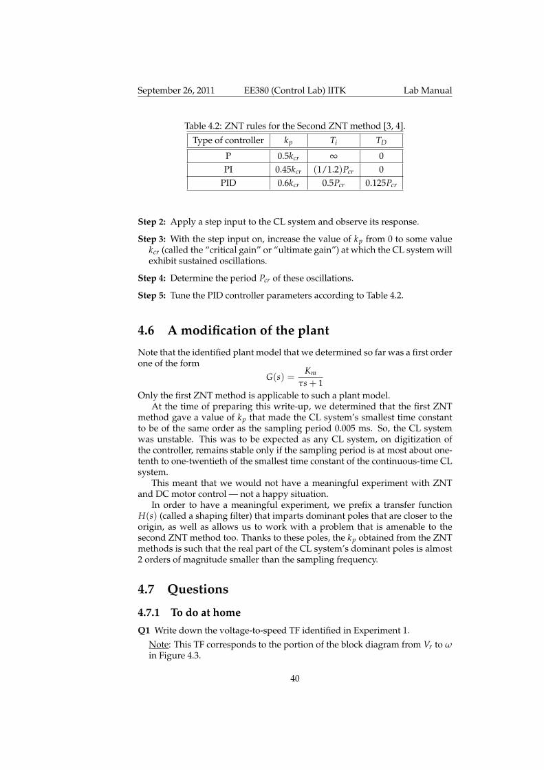
September 26, 2011 EE380 (Control Lab) IITK Lab Manual
Table 4.2: ZNT rules for the Second ZNT method [3, 4].
Type of controller kp Ti TD
P 0.5kcr ∞ 0PI 0.45kcr (1/1.2)Pcr 0
PID 0.6kcr 0.5Pcr 0.125Pcr
Step 2: Apply a step input to the CL system and observe its response.
Step 3: With the step input on, increase the value of kp from 0 to some valuekcr (called the “critical gain” or “ultimate gain”) at which the CL system willexhibit sustained oscillations.
Step 4: Determine the period Pcr of these oscillations.
Step 5: Tune the PID controller parameters according to Table 4.2.
4.6 A modification of the plant
Note that the identified plant model that we determined so far was a first orderone of the form
G(s) =Km
τs + 1Only the first ZNT method is applicable to such a plant model.
At the time of preparing this write-up, we determined that the first ZNTmethod gave a value of kp that made the CL system’s smallest time constantto be of the same order as the sampling period 0.005 ms. So, the CL systemwas unstable. This was to be expected as any CL system, on digitization ofthe controller, remains stable only if the sampling period is at most about one-tenth to one-twentieth of the smallest time constant of the continuous-time CLsystem.
This meant that we would not have a meaningful experiment with ZNTand DC motor control — not a happy situation.
In order to have a meaningful experiment, we prefix a transfer functionH(s) (called a shaping filter) that imparts dominant poles that are closer to theorigin, as well as allows us to work with a problem that is amenable to thesecond ZNT method too. Thanks to these poles, the kp obtained from the ZNTmethods is such that the real part of the CL system’s dominant poles is almost2 orders of magnitude smaller than the sampling frequency.
4.7 Questions
4.7.1 To do at home
Q1 Write down the voltage-to-speed TF identified in Experiment 1.
Note: This TF corresponds to the portion of the block diagram from Vr to ωin Figure 4.3.
40

September 26, 2011 EE380 (Control Lab) IITK Lab Manual
29s2 + 10s + 29
H(s)
u∣∣∣∣ uVs
∣∣∣∣ ≤ 0.8
Saturation
u 1Vs
uactualPWM
δ H-bridge MotorVreq ω
Figure 4.3: Block diagram of the plant for which we wish to tune a PID con-troller. Here, u is controller’s output, uactual is numerical value of voltage ap-plied to motor’s armature. This number is divided by Vs (power supply volt-age equal to 12 V) to obtain the duty ratio δ. δ is input to the PWM moduleof the dsPIC30F4012. The dsPIC outputs a PWM signal to the Solarbotics H-bridge board. The H-bridge board is fed from a DC power supply at a voltageof Vs. The H-bridge board outputs a variable-magnitude DC voltage Vreq tothe DC motor. The transfer function H(s) is not part of the plant model that weidentified in Experiment 1 or 2. We have added the prefilter H(s) here to makethe plant model amenable to ZNT methods, as described in Section 4.6. Notethat the u to ω path shown in this figure is more accurate than that shown inFigure 3.1.
Q2 Prefix H(s) = 29s2+10s+29 to this TF.
Second ZNT method
Q3.1 Determine kcr using rlocus of GNU Octave upto the resolution of thehuman eye. Simulate the CL system in GNU Octave and determine kcr andPcr.
Q3.2 Determine the three controllers (P, PI, PID).
Q3.3 In GNU Octave, simulate the CL step response using tf, conv, step, witheach of these controllers, and fill Table 4.3.
Note 2 The PID controller has a non-proper TF: k1(s + α)2/s. You will not beable to simulate this controller in GNU Octave. To simulate the PID controller, youwill need to add a pole whose real part is about 10 times larger in magnitude thanthe controller zero α, but at least 10 times smaller than the sampling frequency.Here, sampling frequency ωs is calculated in rad/s and equals 2π/Ts, where Ts isthe sampling period.
Q3.4 Based on the values of tr that you have in Table 4.3, and given that thesampling interval is 2 ms, do you think the CL system under digital controlwill be stable?
Q3.5 Repeat Q3.3 using easysim.m and Ts = 2 ms. Is the CL system stable?
Q3.6 From Table 4.3, what are the advantages and disadvantages of each of thethree controllers? Which controller would you select to control your plant?
Q3.7 Is the design specification of QAD satisfied by any of the three con-trollers?
41

September 26, 2011 EE380 (Control Lab) IITK Lab Manual
Table 4.3: Table for Q3.3Value of C(s) tr ess Mp
2nd overshoot1st overshoot
P
PI
PID
Table 4.4: Table for Q6: Results from PID control
Type of experiment tr ess Mp2nd overshoot1st overshoot
Simulation
Practical
Q3.8 Write the Euler’s approximation-based descretized versions of each ofthe three controllers and H(s) in C code. You will take these codes to thelab.
4.7.2 To do in lab: Second ZNT method
Q4 Program the discretized version H(s) in your dsPIC. Use the kcr obtainedin Q3.1. Give a step input and see the CL response. Do you think that itprovides sustained oscillations of the CL system? If it does not, then tunekcr until you hit a value that provides sustained oscillations. Note this valueand the value of Pcr.
Q5 With the value of kcr and Pcr that you determined in Q4, form a PID con-troller.
Note 3 Note 2 applies here too.
Q6 Check using GNU Octave and easysim.m that this PID controller works.Note its performance in Table 4.4.
Q7 Program the digital controller from Q6 into the dsPIC and run the setup.Record the results in Table 4.4. Plot the necessary data.
Q8 Explain the differences between practice and simulation, if any.
42

Chapter 5
Experiment 4: Control ofspeed using armature current
5.1 Goals
To control the speed of the pmdc motor using feedback of current.
5.2 Application of this problem
The area of sensorless speed control (SSC) uses the measurements of the voltageV applied to the armature, and one of either armature current i or back emf E,to estimate the motor speed ω:
1. Back emf speed control: V is turned alternatively on and off, as in the case ofour H-bridge circuit. During the on period, the motor gathers speed. Duringthe off period, a brief period is allowed to elapse until i dies down while therotor is coasting, and then the voltage is measured across the armature. Thisvoltage is the estimate E of the back emf. Then the estimate ω of ω can beobtained as E/Kb. Note that i is not measured in this method.
Commerical controllers, such as [7], exist for SSC of dc motor using feedbackof back emf. Also, see, for example, [8] for some details.
2. Speed control using armature current: An estimate of the back emf is obtainedby measuring the armature current i and using the expression E = V − R∑i.
Commercial controllers, such as [9], exist for SSC of pmdc motor using IRcompensation. Also, see, for example, [10] for some details.
The advantage of SSC is that V and i can be measured using componentsthat are fixed in the motor circuit. On the other hand, speed is measured usingdevices, such as encoders or tachogenerators. There are several drawbacks inusing these devices such as increased volume of the motor unit and loweredreliability as the encoders may go bad earlier than the motors. The latter draw-back may be particularly significant where repair may not be possible, such asin space applications.
43

September 26, 2011 EE380 (Control Lab) IITK Lab Manual
S1 S2
S3 S4
Vs
Rs
Motor
S1 S2
S3 S4
Vs
Rs
Motor
Figure 5.1: How the H-bridge is used to switch the direction of rotation of themotor shaft. With the switches S2 and S3 open, the pulse width modulatedjoint opening and closing of switches S1 and S4 make the motor turn in onedirection with varying speed. Similarly, with the switches S1 and S4 open,and S2 and S3 closing jointly by the PWM signal the motor turns in the otherdirection. In either direction, the effective resistance of the motor’s armatureincludes the resistance RH of the two closed switches, the resistance Rs of thesensing resistor, and the resistance Rm of the motor armature, as mentionedin Section 1.4.2. Also, the Vreq of Figure 4.3 is actually the time average of thePWM voltage seen between the terminal labeled Vs and the above diagram,and not the voltage immediately across the motor terminals.
5.3 Background
The equations that describe a pmdc motor are
V = Ldidt
+ Ri + E (5.1)
Jdω
dt= −Bω + T − TL (5.2)
Here, T = KTi and E = Kbω. Depending on the situation, the load torqueTL may either be treated as a disturbance or as an input. In this experiment, wewill treat it as a disturbance. We have, V is the Vreq of Figure 4.3.
The resistance R needs to be seen between the terminals across which the
44

September 26, 2011 EE380 (Control Lab) IITK Lab Manual
ωref +Controller
uMotor module
ω
+RΣ
isens−1
Kbω
−
Figure 5.2: Block diagram of control of speed using feedback of armature cur-rent.
voltage V is applied. As explained in Figure 5.1, R = RΣ. Therefore, we have
V = Ldidt
+ R∑i + E
We see from Figure 2.1 that there are two time constants in the V to ωtransfer function of the pmdc motor. These are the electrical time constantτe = La/RΣ and the mechanical time constant τm = J/B. As a rule of thumb,in a general pmdc motor, τe is about one tenth τm. However, in our case, the τeis 1.9× 10⁻⁵ s, while τm is 0.44 s. That is, transients in i settle about 104 times asfast as transients in ω, meaning that τe be ignored without any loss of accuracy.
To remove τe from discussion, we set L = 0, resulting in V = RΣi + Kbω.This equation shows that, when τe ≈ 0, ω can be calculated as ω = V−RΣi
Kb. We
can use this equation to determine ω and use this estimate for feedback controlof ω as shown in Figure 5.2.
5.4 Questions
5.4.1 To do at home
1. Using the values of Km and τm that you determined from the OL step re-sponse in Experiment 1, determine the values of B and RΣ as follows.
Solve equations (2.2) and (2.3) simultaneously to determine the values ofR∑ = RH + Rm + Rsens and B. Use the values of J, KT , Kb from Table 1.1. Donot use the value of B calculated in Section 1.4.1.
Remark 1 The equivalent internal resistance (RH) of the L298 as measured bySolarbotics is as follows1:
IC voltage
9 V 12 V 18.95 V
Equivalent internal resistance (Ω) 2.86 2.39 2.00
However, our results of Experiment 1 give us a value of RH that is quite differentfrom what the above table says.1Page 9 of solarbotics_l298_compact_motor_driver_kit.pdf that is available at
http://www.solarbotics.com/products/k_cmd/resources/
45

September 26, 2011 EE380 (Control Lab) IITK Lab Manual
2. Write down the controller that you designed in Experiment 1.
3. Simulate your closed-loop control of motor speed in two ways under thiscontroller using a modification of easysim.m:
3.1. Using feedback of current with ω = u−RΣiKb
, and
3.2. Using feedback of speed.
Plot ω and ω on one figure.
5.4.2 To do in lab
4. Verify that your experimental setup is connected as appropriate for this ex-periment.“Appropriate” here means that the lead from the sensing resistor Rs needsto be connected to CN4 input pin 1 as shown in Figure 5.3, apart from theusual connections for speed control.
5. Write a code to apply a step input to the motor. Run the setup in OL mode.
6. Identify the system parameters Km and τm by using the OL step response.
7. If Km and τm are different from those you saw in Experiment 1, calculate thevalues of RΣ and B as you did in Question 1.Else, in the following, use the RΣ determined at home.
8. Uncomment the following part of main-prog.c
/*IV = AD_value(); // Read voltage across Rs=4.7ohm.IV = 5*(511 + IV)/1022; // Convert signed to unsigned.I[1] = IV/4.7; // Convert voltage to current.
// Low-pass filter with cut-off frequency wf:IF[1] = (wf*T/(2+wf*T))*(I[1]+I[0])+((2-wf*T)/(2+wf*T))*IF[0];// Prepare IF[0] and I[0] for the next sampling intervalIF[0] = IF[1];I[0] = I[1];
*/
This code is explained in Section 5.5.
9. Control the motor in three ways:
9.1. Using feedback of speed (as in Experiment 1).9.2. Using feedback of current with ω = (u− RΣisens)
/Kb, and
9.3. Using feedback of current with ω =(
u− RΣ i)/
Kb, where, i ≈1
1.8 isens − 130 .
See Figure 1.6 for an explanation of this relation between i and isens.You may need to tweak this relation between i and isens for your ownsetup to obtain satisfactory results. See Section 5.6 for a systematic andtime-saving way to determine the relation between i and isens.
46

September 26, 2011 EE380 (Control Lab) IITK Lab Manual
Encoder
M
Rs=
4.7Ω
L29
8
+-
DB9-UART-A
CN2-PICKIT2 DB9-CAN
5
I s
FG C
CN
1-PS
CN4-I/P CN5-O/P CN3-Motor
µCbo
ard
+12
V
H-b
ridg
ebo
ard
I 1I 2
E1−
2
+-−1
2V+
12V
GN
D
I 3I 4
E3−
4G
ND
+5V
+V
cc
M2
M1
M3
M4
101 1 3 5-9
1
PICKIT2
RS2
32 USB
PC
Figu
re5.
3:C
onec
tion
diag
ram
ofth
ese
tup.
InEx
peri
men
t2,a
sign
alfr
omth
eFG
was
inpu
tatc
onne
ctor
CN
4-I/
Pof
the
µC
boar
d.O
nth
eot
her
hand
,in
the
pres
ente
xper
imen
t,th
em
otor
curr
enti
sin
stea
din
puta
tthi
sco
nnec
tor.
The
capa
cito
rC=
1000
µF.
47

September 26, 2011 EE380 (Control Lab) IITK Lab Manual
Plot ω and ω from the three types of control on one figure. Of course, in thefirst case, ω is absent.
10. In the control of motor speed, is the feedback of armature current an ade-quate substitute for the feedback of motor speed?
11. Write in your lab reports the code that you inserted into main-prog.c ineach of the above two ways.
5.5 Explanation for the C code related to currents
5.5.1 Reading the current through ADC
Here we explain the following C code.
IV = AD_value(); // Read voltage across Rs=4.7ohm.IV = 5*(511 + IV)/1022; // Convert signed to unsigned.I[1] = IV/4.7; // Convert voltage to current.
The 10-bit ADC in dsPIC30F4012 is capable of working with inputs in therange [0, 5] V. There are two modes in which this ADC can work. These aresigned and unsigned modes. In signed mode the ADC maps [0, 5] V to the inter-val [−511,+511]. In the unsigned mode the ADC maps [0, 5] V to [0,+1023].
With the experiment involving tracking a sinusoid in mind, we config-ured the ADC to work in the signed mode. This configuration is done insettings-prog.h that we keep unchanged throughout our lab. When we wishto output unipolar signals from the ADC, we can either (a) reconfigure it in un-signed mode or (b) allow it to work in signed mode, but provide an offset to itsouput.We take this second approach in the above code. v
5.5.2 Software-based low pass filter for isens
Here we explain the first line of the following C code:
// Low-pass filter with cut-off frequency wf:IF[1] = (wf*T/(2+wf*T))*(I[1]+I[0])+((2-wf*T)/(2+wf*T))*IF[0];// Prepare IF[0] and I[0] for the next sampling intervalIF[0] = IF[1]; I[0] = I[1];
The following low pass filter for isens is present in main-prog.c
I f (s)I(s)
=ω f
s + ω f(5.3)
Here we explain how it has been coded into main-prog.c.Instead of the method of going from the TF to the SS model to the dis-
cretized equations, we use the method of going from s-domain TF to z-domainTF to the discretized equations.
We go from s-domain to the z-domain using s = 2Ts
z−1z+1 (the bilinear trans-
form) to obtainI f (z)I(z)
=ω f Ts
(1 + z−1)
2 (1− z−1) + ω f Ts (1 + z−1)
48

September 26, 2011 EE380 (Control Lab) IITK Lab Manual
This equation can be rewritten as(2(
1− z−1)+ ω f Ts
(1 + z−1
))I f (z) = ω f Ts
(1 + z−1
)I(z),
that is, as
2I f (z)− 2z−1 I f (z) + ω f Ts I f (z) + ω f Tsz−1 I f (z) = ω f Ts I(z) + ω f Tsz−1 I(z)
Taking the inverse Z-transform (Z−1) on both sides of the last equation, wehave
2i f (k)− 2i f (k− 1) + ω f Tsi f (k) + ω f Tsi f (k− 1) = ω f Tsi(k) + ω f Tsi(k− 1).
The expression for i f (k) in terms of i f (k− 1), i(k), and i(k− 1) is
i f (k) =ω f Ts
2 + ω f Ts(i(k) + i(k− 1)) +
2−ω f Ts
2 + ω f Tsi f (k− 1)
This equation is the first line of the above code.
5.6 Systematic method to determine i versus isens
For whatever reasons, isens in the block diagram of Figure 5.2 is not equal to i,the armature current. From Figure 1.6 that we obtained through certain trialsbefore we developed these experiments, we estimated that
isens =1
a(TL)i− b(TL)
a(TL)
Thus, we can construct an estimate i of i using isens as
i = a(TL)isens + b(TL)
and use this estimate to construct ω as
ω =V − RΣ i
Kb.
How to determine a and b? As we have two unknowns at each value of TL,we need two equations in these unknowns. We can proceed as follows.
Step 1 Construct ω as shown in Figure 5.4.From this figure, we see that
ω(s) =[
U(s)−(
I(s)a− b
as
)RΣ
]1
Kb,
withI(s) =
1/RΣ
1 + KtKbRΣ(Js+B)
U(s)
For u(t) being a step input of um V, the steady state value of ω is
ωssum =
[um −
um/a
1 + KtKbRΣB
+bRΣ
a
]1
Kb(5.4)
In this equation, Kt, Kb, RΣ, B are known.
49

September 26, 2011 EE380 (Control Lab) IITK Lab Manual
U(s) + 1RΣ
I(s)Kt
T(s) +
TL(s)
− 1Js + B
ω(s)
Kb
−
1/a
+ba
1(t) −
RΣ
isens
−+1/Kb
ω
The part outside dsPIC30F4012
Figure 5.4: Block diagram to illustrate the procedure of Section 5.6.
Step 2 Apply u(t) of a known magnitude and measure the correspondingωssum . Then, only a and b remain as the unknowns in (5.4).
Thus, for example, for um = 7 V, we have the equation
a(Kbωss7 − 7) = RΣb− 7α
, where α = 1 +KtKbRΣB
.
and for um = 9 V, we have the equation
a(Kbωss9 − 9) = RΣb− 9α
.
Assuming that these two equations are linearly independent, we have[b
a
]=
[RΣ 7− Kbωss7
RΣ 9− Kbωss9
]−1 [7
9
]× α
Remark 2 Ideally, we need to determine a and b for a series of values of TL. But, inour experiment, we restrict ourselves to TL = 0.
Remark 3 To determine ωssum see if it is not enough to observe this value from onlythe terminal.log file. This may save you the trouble of plotting ω.
5.7 Post-experiment discussion
In the experiment with ωref = 100 rad/s, we found that in Question 9.2, ω ≈100 rad/s and ω ≈ 50 rad/s, while in Question 9.3, in the best case, ω ≈ 100
50

September 26, 2011 EE380 (Control Lab) IITK Lab Manual
rad/s and ω ≈ 70 rad/s. Clearly, much improvement is needed. Prof. AvinashJoshi suggested that such a large error is most likely due to even small errorsin the i — isens relationship used, or the neglected constant voltage drop acrossthe brushes, etc. We need to pursue this line of investigation.
Thanks 1 We thank Prof. Avinash Joshi for discussing with us the results of thisexperiment. From this discussion, we learned that what we are doing in this exper-iment goes under the name of speed control using IR compensation, and that IRcompensation, and thereby the speed control, is indeed difficult.
51

September 26, 2011 EE380 (Control Lab) IITK Lab Manual
52

Chapter 6
Experiment 5: Control ofarmature current
6.1 Goals
To control the armature current of the pmdc motor at the desired value.
6.2 Application of the problem
The disturbance observer (DOB) that we see in Experiment 6 requires the arma-ture current of the pmdc motor to be well-regulated. In the present experiment,we attempt to make the armature current well-regulated.
Apart from the application in the DOB, a current loop, when present, is theinnermost loop in electric drives, the next outer one being the speed controlloop, followed by the position control loop, which is also the outermost loopas shown in Figure 6.1. This three-loop structure is used also with motors otherthan pmdc. This structure is used for tracking a given θd while restricting thespeed or current. When only control of speed is needed while constraining thecurrent, the outer-most loop can be removed. See, for example, [11, page 36].
6.3 Well-regulated current
Figure 6.2 shows the block diagram of the pmdc motor under control of arma-ture current. Figure 6.3 shows this block diagram redrawn. Figure 6.3 showsthat i cannot track id alone, but only id − iex. i will be considered as well-regulated if it tracks id nicely. i will not track id nicely as long as iex dominates.
If Ki(s) has poles, then Kb/Ki(s) will contain zeros. Zeros represent deriva-tive elements. Especially during transients in ω, these zeros will differentiateω with respect to time, leading to a large value of iex, and consequently to largeerrors between id and i. Also, these zeros amplify sensor noise. Therefore, weprefer for 1/Ki(s) not to have zeros. However, if we do not have a choice, thenwe need to use a filter on isens, which is the sensed version of i. This filter is
53
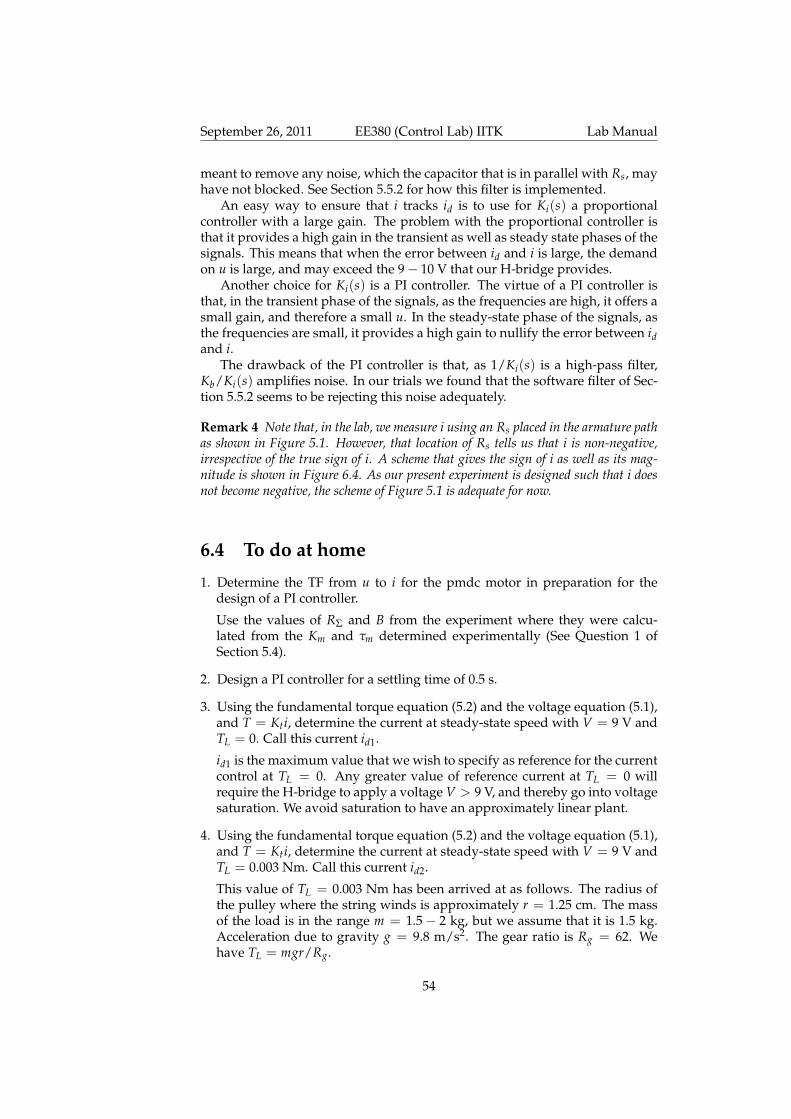
September 26, 2011 EE380 (Control Lab) IITK Lab Manual
meant to remove any noise, which the capacitor that is in parallel with Rs, mayhave not blocked. See Section 5.5.2 for how this filter is implemented.
An easy way to ensure that i tracks id is to use for Ki(s) a proportionalcontroller with a large gain. The problem with the proportional controller isthat it provides a high gain in the transient as well as steady state phases of thesignals. This means that when the error between id and i is large, the demandon u is large, and may exceed the 9− 10 V that our H-bridge provides.
Another choice for Ki(s) is a PI controller. The virtue of a PI controller isthat, in the transient phase of the signals, as the frequencies are high, it offers asmall gain, and therefore a small u. In the steady-state phase of the signals, asthe frequencies are small, it provides a high gain to nullify the error between idand i.
The drawback of the PI controller is that, as 1/Ki(s) is a high-pass filter,Kb/Ki(s) amplifies noise. In our trials we found that the software filter of Sec-tion 5.5.2 seems to be rejecting this noise adequately.
Remark 4 Note that, in the lab, we measure i using an Rs placed in the armature pathas shown in Figure 5.1. However, that location of Rs tells us that i is non-negative,irrespective of the true sign of i. A scheme that gives the sign of i as well as its mag-nitude is shown in Figure 6.4. As our present experiment is designed such that i doesnot become negative, the scheme of Figure 5.1 is adequate for now.
6.4 To do at home
1. Determine the TF from u to i for the pmdc motor in preparation for thedesign of a PI controller.
Use the values of RΣ and B from the experiment where they were calcu-lated from the Km and τm determined experimentally (See Question 1 ofSection 5.4).
2. Design a PI controller for a settling time of 0.5 s.
3. Using the fundamental torque equation (5.2) and the voltage equation (5.1),and T = Kti, determine the current at steady-state speed with V = 9 V andTL = 0. Call this current id1.
id1 is the maximum value that we wish to specify as reference for the currentcontrol at TL = 0. Any greater value of reference current at TL = 0 willrequire the H-bridge to apply a voltage V > 9 V, and thereby go into voltagesaturation. We avoid saturation to have an approximately linear plant.
4. Using the fundamental torque equation (5.2) and the voltage equation (5.1),and T = Kti, determine the current at steady-state speed with V = 9 V andTL = 0.003 Nm. Call this current id2.
This value of TL = 0.003 Nm has been arrived at as follows. The radius ofthe pulley where the string winds is approximately r = 1.25 cm. The massof the load is in the range m = 1.5− 2 kg, but we assume that it is 1.5 kg.Acceleration due to gravity g = 9.8 m/s2. The gear ratio is Rg = 62. Wehave TL = mgr/Rg.
54
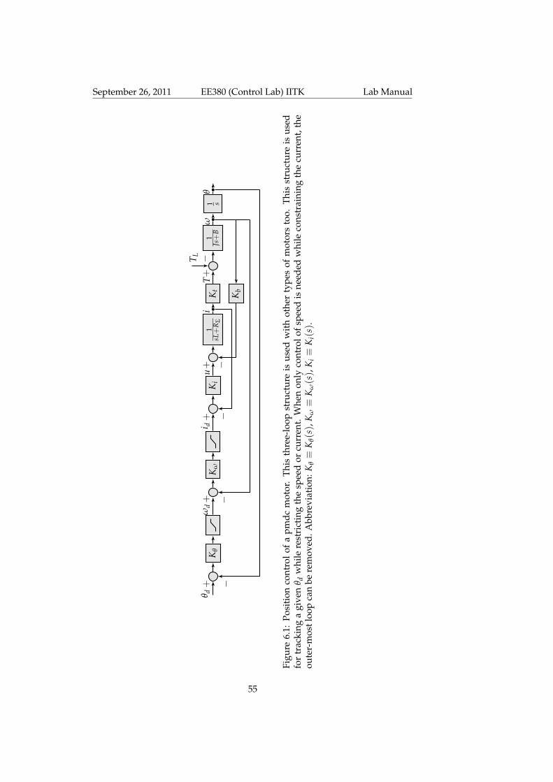
September 26, 2011 EE380 (Control Lab) IITK Lab Manual
θ d+
Kθ
ωd+
Kω
i d+
Ki
u+
1sL+
RΣ
iK
tT+
T L −1
Js+
Bω
1 s
Kb
−−
θ
−−
Figu
re6.
1:Po
siti
onco
ntro
lof
apm
dcm
otor
.Th
isth
ree-
loop
stru
ctur
eis
used
wit
hot
her
type
sof
mot
ors
too.
This
stru
ctur
eis
used
for
trac
king
agi
ven
θ dw
hile
rest
rict
ing
the
spee
dor
curr
ent.
Whe
non
lyco
ntro
lofs
peed
isne
eded
whi
leco
nstr
aini
ngth
ecu
rren
t,th
eou
ter-
mos
tloo
pca
nbe
rem
oved
.Abb
revi
atio
n:K
θ≡
Kθ(s),
Kω≡
Kω(s),
Ki≡
Ki(
s).
55

September 26, 2011 EE380 (Control Lab) IITK Lab Manual
id +Ki(s)
u + 1sL + RΣ
iKt
T +
TL
− 1Js + B
ω
Kb
−−
Plant: The part outside dsPIC30F4012
Figure 6.2: Control of current in a pmdc motor. For the design of the controllerKi(s) of current, use the values of RΣ, B that you determined in Question 1 ofSection 5.4. Note that Ki(s) does not stand for an integral controller. Instead, itis the controller for i, the armature current.
id + +Ki(s)
1sL + RΣ
iKt
T +
TL
− 1Js + B
ω
KbKi(s)iex
− −
Figure 6.3: The block diagram of Figure 6.2 redrawn. We can see that i tracksid − iex, and not id alone. i is considered well-regulated if it tracks id nicely.This nice tracking will not happen while iex dominates. Therefore, we chooseKi(s) to supress iex. Two choices for Ki(s) are P and PI.
This id2 is the maximum value that we wish to specify as reference for thecurrent control at TL = 0.003 Nm. Any greater value of reference current atTL = 0.003 Nm will require the H-bridge to apply a voltage V > 9 V, andthereby go into voltage saturation. We avoid saturation to have an approx-imately linear plant. The minimum value of id2 is TL/Kt. When we applythe load and require the motor to track a value of id that is less than thisminimum value of id2, the load will drive the motor, rather than the motordriving the load.
5. Simulate the CL system of Figure 6.2 using a modification of easysim.m for
5.1. id = id1, and
5.2. id = id2.
6. Plot the i versus t and u versus t curves from parts 5.1 and 5.2.
6.5 To do in lab
7. Write the discretized version of the home-designed controller intomain-prog.c. In main-prog.c implement the part of the block diagram ofFigure 6.2 that is outside the plant. Either use the expression for i in terms
56
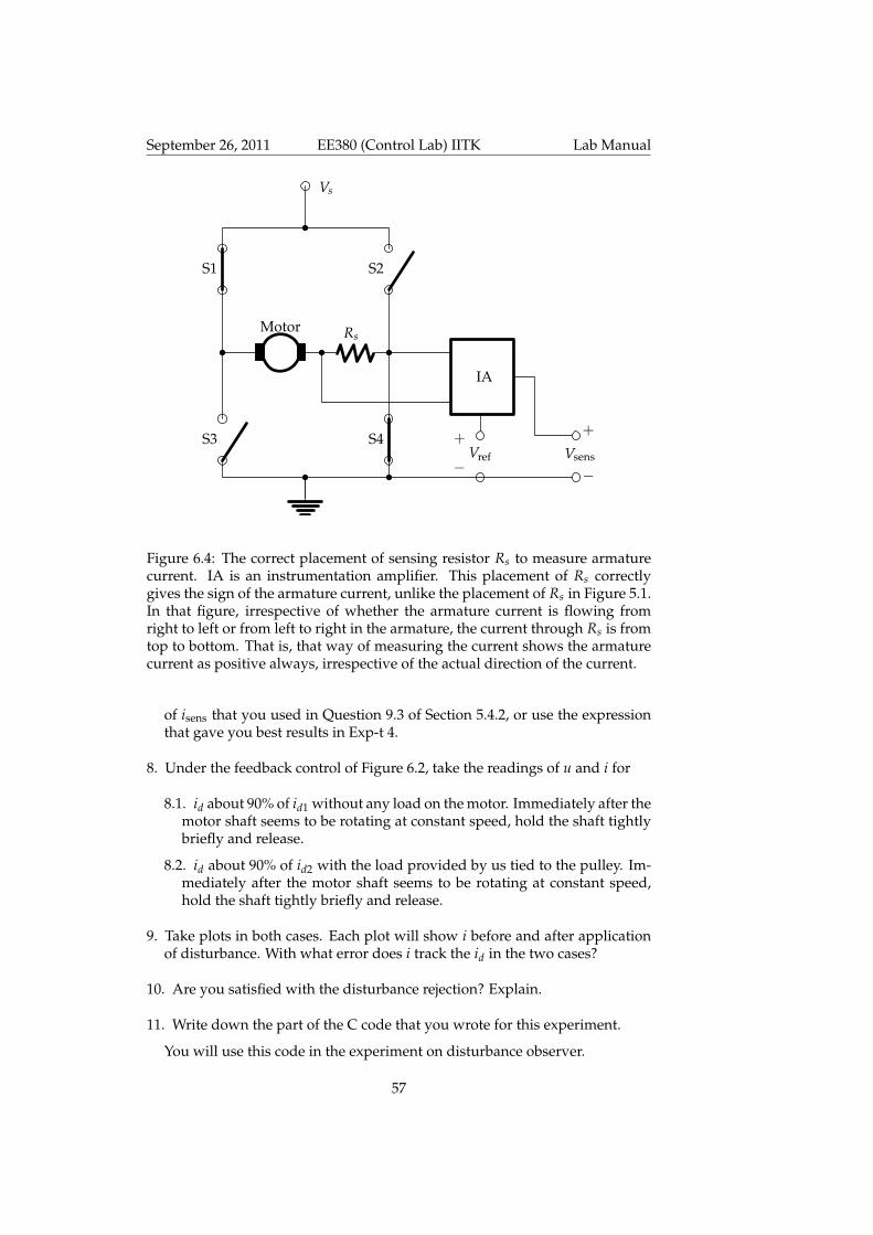
September 26, 2011 EE380 (Control Lab) IITK Lab Manual
Vs
RsMotor
IA
Vsens
S2S1
S3 S4Vref
−
+
−
+
Figure 6.4: The correct placement of sensing resistor Rs to measure armaturecurrent. IA is an instrumentation amplifier. This placement of Rs correctlygives the sign of the armature current, unlike the placement of Rs in Figure 5.1.In that figure, irrespective of whether the armature current is flowing fromright to left or from left to right in the armature, the current through Rs is fromtop to bottom. That is, that way of measuring the current shows the armaturecurrent as positive always, irrespective of the actual direction of the current.
of isens that you used in Question 9.3 of Section 5.4.2, or use the expressionthat gave you best results in Exp-t 4.
8. Under the feedback control of Figure 6.2, take the readings of u and i for
8.1. id about 90% of id1 without any load on the motor. Immediately after themotor shaft seems to be rotating at constant speed, hold the shaft tightlybriefly and release.
8.2. id about 90% of id2 with the load provided by us tied to the pulley. Im-mediately after the motor shaft seems to be rotating at constant speed,hold the shaft tightly briefly and release.
9. Take plots in both cases. Each plot will show i before and after applicationof disturbance. With what error does i track the id in the two cases?
10. Are you satisfied with the disturbance rejection? Explain.
11. Write down the part of the C code that you wrote for this experiment.
You will use this code in the experiment on disturbance observer.
57

September 26, 2011 EE380 (Control Lab) IITK Lab Manual
6.6 What to check if things do not work
If you seem to have done everything correctly, and yet your control system isnot working the way it should, here are some points you can check.
1. Is the electrolytic capacitor connected with correct polarity, as shown in Fig-ure 5.3?
Thanks 2 We thank Prof. Shyama Prasad Das for helping us formulate questions 3and 4.
58

Chapter 7
Experiment 6: Disturbanceobserver
7.1 Goal
To implement a disturbance observer (DOB) for a pmdc motor.
7.2 Background
7.2.1 Application of DOB
A conventional forward path controller such as P, PI, PID, lead, lag, etc, whichis a single degree of freedom controller (see Figure 7.1 (a)), can reject disturbancesas well as provide good performance if designed and tuned properly. Thedesign and tuning becomes much easier with a so-called two-degree of freedom(2DOF) controller (Figure 7.1 (b)). There are two parts to this controller, each ofwhich can be designed and tuned independent of the other.
7.2.2 Model of pmdc motor with well-regulated current
For the case where the developed torque T is proportional to a current i asT = Kti, and where this current is well-regulated at the desired value id, asdone in Figure 6.2, the motor-gear unit can be represented as in Figure 7.2.
For example, NASA’s Mars rovers used brushed dc motors (same as pmdcmotors) as their driving and steering motors [12]. For these motors, i is the ar-mature current. Brushless dc (bldc) motors are also an alternative, for example,in the Lunar Rover that ISRO has built in-house and that IITK has also built.For bldc motors i is the average dc link current [13, page 769].
7.2.3 DOB for a pmdc motor with well-regulated current
TL can be estimated through either the OL scheme or the CL scheme of Fig-ure 7.3. By working out the transfer functions from TL to TL in these two
59
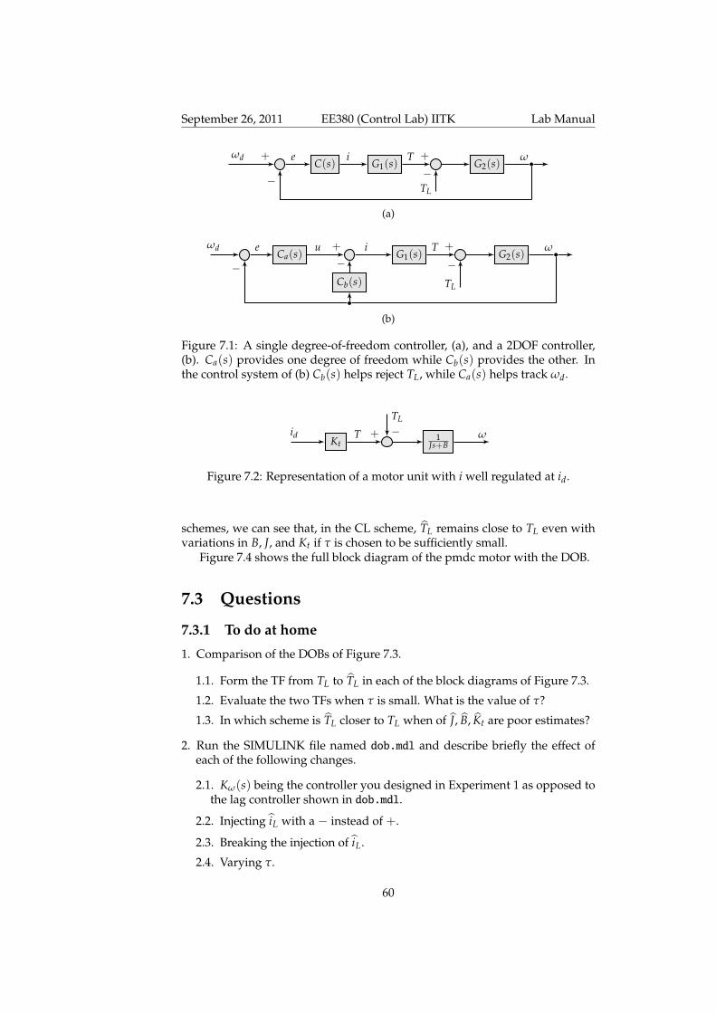
September 26, 2011 EE380 (Control Lab) IITK Lab Manual
ωd +C(s)
eG1(s)
i T +
TL
−G2(s)
ω
−
(a)
ωdCa(s)
e u +G1(s)
i T +
TL
−G2(s)
ω
Cb(s)− −
(b)
Figure 7.1: A single degree-of-freedom controller, (a), and a 2DOF controller,(b). Ca(s) provides one degree of freedom while Cb(s) provides the other. Inthe control system of (b) Cb(s) helps reject TL, while Ca(s) helps track ωd.
Ktid T +
TL
−1
Js+Bω
Figure 7.2: Representation of a motor unit with i well regulated at id.
schemes, we can see that, in the CL scheme, TL remains close to TL even withvariations in B, J, and Kt if τ is chosen to be sufficiently small.
Figure 7.4 shows the full block diagram of the pmdc motor with the DOB.
7.3 Questions
7.3.1 To do at home
1. Comparison of the DOBs of Figure 7.3.
1.1. Form the TF from TL to TL in each of the block diagrams of Figure 7.3.
1.2. Evaluate the two TFs when τ is small. What is the value of τ?
1.3. In which scheme is TL closer to TL when of J, B, Kt are poor estimates?
2. Run the SIMULINK file named dob.mdl and describe briefly the effect ofeach of the following changes.
2.1. Kω(s) being the controller you designed in Experiment 1 as opposed tothe lag controller shown in dob.mdl.
2.2. Injecting iL with a − instead of +.
2.3. Breaking the injection of iL.
2.4. Varying τ.
60
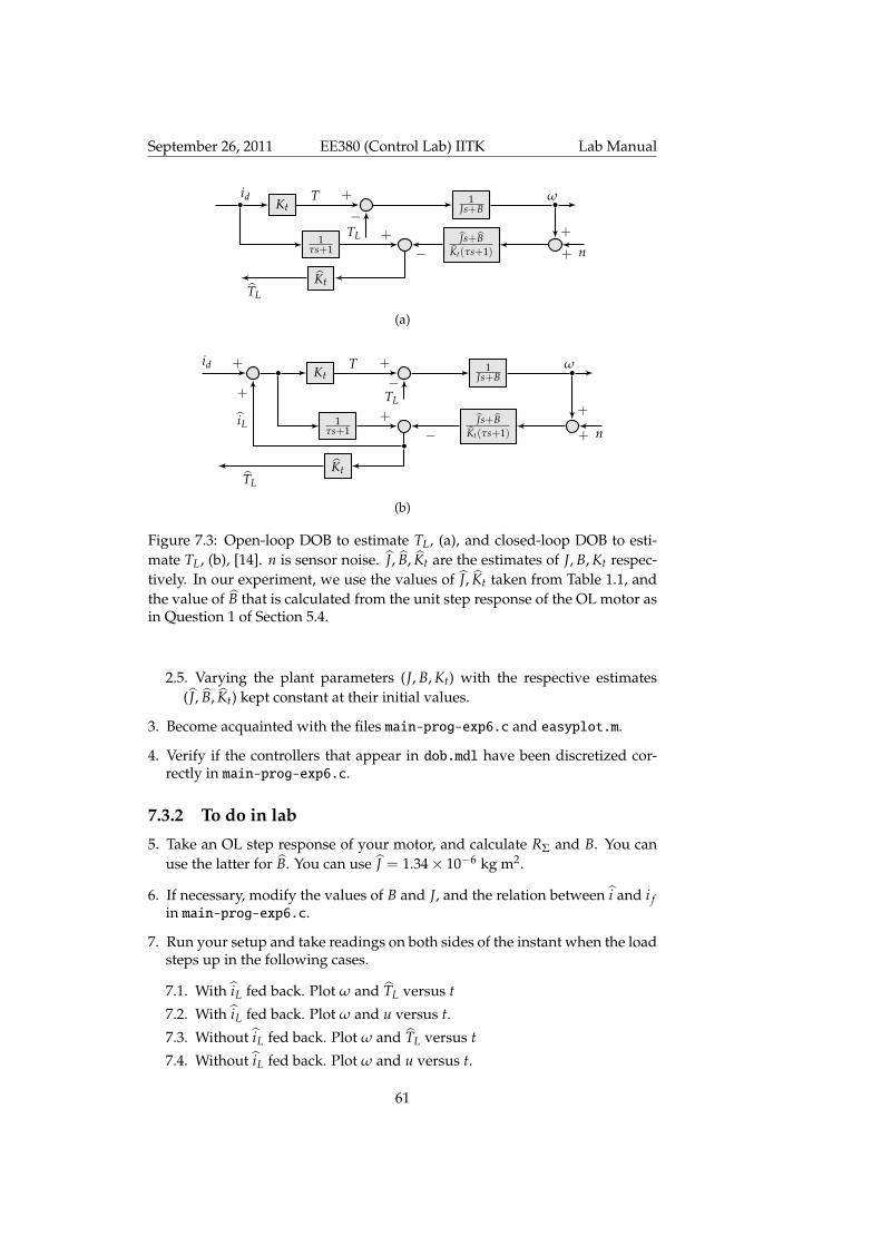
September 26, 2011 EE380 (Control Lab) IITK Lab Manual
Ktid T +
TL
−1
Js+Bω
+
n+Js+B
Kt(τs+1)−1
τs+1+
KtTL
(a)
id +Kt
T +
TL
−1
Js+Bω
+
n+Js+B
Kt(τs+1)−1
τs+1+
KtTL
iL
+
(b)
Figure 7.3: Open-loop DOB to estimate TL, (a), and closed-loop DOB to esti-mate TL, (b), [14]. n is sensor noise. J, B, Kt are the estimates of J, B, Kt respec-tively. In our experiment, we use the values of J, Kt taken from Table 1.1, andthe value of B that is calculated from the unit step response of the OL motor asin Question 1 of Section 5.4.
2.5. Varying the plant parameters (J, B, Kt) with the respective estimates( J, B, Kt) kept constant at their initial values.
3. Become acquainted with the files main-prog-exp6.c and easyplot.m.
4. Verify if the controllers that appear in dob.mdl have been discretized cor-rectly in main-prog-exp6.c.
7.3.2 To do in lab
5. Take an OL step response of your motor, and calculate RΣ and B. You canuse the latter for B. You can use J = 1.34× 10⁻⁶ kg m2.
6. If necessary, modify the values of B and J, and the relation between i and i fin main-prog-exp6.c.
7. Run your setup and take readings on both sides of the instant when the loadsteps up in the following cases.
7.1. With iL fed back. Plot ω and TL versus t
7.2. With iL fed back. Plot ω and u versus t.
7.3. Without iL fed back. Plot ω and TL versus t
7.4. Without iL fed back. Plot ω and u versus t.
61

September 26, 2011 EE380 (Control Lab) IITK Lab Manual
ωd
+K
ω(s)
id+
+K
i (s)u
+1
sL+
RΣ
iK
tT
+
TL
−1
Js+B
Inertiaω
Kb
−−
Js+B
Kt (τs+
1)
Inverseinertia
1τs+
1
Filtery
1+
y2
−
iL +−
Thispartis
implem
entedin
experimenttitled
“Controlofarm
aturecurrent”
Figure7.4:T
hefullblock
diagramofthe
two-degree
offreedomcontrolofa
pmdc
motor.The
firstdegreeoffreedom
isprovided
bythe
DO
Bin
theinner
loop.The
seconddegree
offreedom
isprovided
bythe
speedcontroller
Kω(s)
thatis
inthe
outerloop.
Theshaded
portionof
theblock
diagramis
implm
entedin
dsPIC30F4012.
Thepurpose
ofthe
filter1/
(τs+
1)is
tonot
justm
akethe
inversionof
1Js+
Bpractically
possible,butalsoto
improve
thedisturbance
rejectionperform
anceofthe
system.See
[14]fordetails.
62

September 26, 2011 EE380 (Control Lab) IITK Lab Manual
The m-file easyplot.m organizes these plots as demonstrated in the lecture.You only need to know how to use it. Make a few trial runs to obtain bestpossible plots.
8. How did you expect your DOB to work? How did it actually work?
7.4 Programs provided
You are provided with the following files:
1. dob.mdl: This SIMULINK file simulates the full block diagram of Figure 7.4.
2. main-prog-exp6.c: This file implements the block diagram in C code. Thisfile implements the block diagram of Figure 7.5.
3. easyplot.m: This m-file helps plot the results read into the PC intoterminal.log by terminal.exe from the µC.
63

September 26, 2011 EE380 (Control Lab) IITK Lab Manual
ωd
+K
ω(s)
iref+
+K
i (s)u
+1
sL+
RΣ
iK
tT
+
TL
−1
Js+B
Inertiaω
Kb
−
φ(i)
ωcf
s+ω
cf
isens
φ −1(if )
if
Js+B
Kt (τs+
1)
Inverseinertia
1τs+
1Filter
i
−
y1
+
y2
−
iL +−
Figure7.5:
The
fullblockdiagram
ofthe
two
degreeof
freedomcontrolsystem
asim
plemented
inour
lab.The
shadedportion
ofthe
blockdiagram
isim
plemented
inmain-prog-exp6.c.
64

Chapter 8
Experiment 7: Disturbanceobserver without feedback ofcurrent
8.1 Goal
To build and test a pmdc motor speed control system that uses a disturbanceobserver (DOB) but does not use the feedback of armature current.
8.2 Background
In Experiment 6, we design a DOB using the feedback of armature current i. Inthe present experiment, we build a slightly modified version of that DOB thatdoes not use the feedback of i.
Figure 8.1 (b) shows the block diagram of Figure 7.4 simplified. Figure 7.4 isreproduced for convenience as Figure 8.1 (a). The advantage of the simplifiedblock diagram is that it does not need the measurement of current if we havethe measurement of speed. The disadvantage is that we do not have TL. Inapplications where we need TL, we need to implement the scheme of Figure 8.1(a), and not the simplified one.
From the SIMULINK model, that we we see that if we replace 1τs+1 with
1 in the path from i to y1, then there is no visible change in the behavior ofthe overall system. Thus, after performing this replacement, the overall blockdiagram can be redrawn as in Figure 7.4 (b).
In our lab, we will implement the scheme of Figure 7.4 (b). One reasonfor this is that scheme (a) needs us to have measurement of current i. Thisquantity, in our experiments, is of the order of a few tens of milliamps andcontains significant amount of noise. In the dual-motor ball-beam setup thatwe built in the Networked Control Systems Lab, we used a capacitor across thesensing resistor to remove this noise, and an instrumentation amplifier to boostthe resultant signal. In the Control Systems Lab, however, we have not yetimplemented this filter-amplifier combination. So, measurements of current
65

September 26, 2011 EE380 (Control Lab) IITK Lab Manual
are not yet accurate enough for feedback.
8.3 Questions
8.3.1 To do at home
1. Play with the SIMULINK file named dobgm.mdl to acquaint yourselves withthe two-degree of freedom control system with the DOB. Some items of in-terest are
1.1. What is the effect of Kω(s) being a PI controller as opposed to a lagcontroller?
1.2. What is the effect of KI(s) being a PI controller as opposed to a propor-tional controller?
1.3. What is the effect of injecting iL with a − instead of +?
1.4. What is the effect of break the injection of iL?
1.5. What is the effect of varying τ?
1.6. What is the effect of varying the plant parameters (J, B, R, Kt) with therespective estimates ( J, B, Kt) kept constant at their initial values?
2. Write the equations that describe the overall closed-loop system of Fig-ure 7.4 (b).
3. Discretize these equations.
4. Check if your discretized equations match what we gave you in the attachedm-file expt6.m.
5. If everything matches, then run the expt6.m in GNU Octave.
6. Write the C code of the controllers that you will implement in the lab.
8.3.2 To do in lab
7. Take an OL step response of your motor, and calculate RΣ and B. You canuse the latter for B. You can use J = 1.34× 10⁻⁶ kg m2.
8. Modify the values in the C code from Question 6, if necessary.
9. Write your C code into the appropriate place in the main-prog.c
10. Run your setup and take readings on both sides of the instant when theload steps up. Provide the following two plots as subplots one below theother: u versus t, and ω versus t.
11. How did you expect your DOB to work? How did it actually work?
66
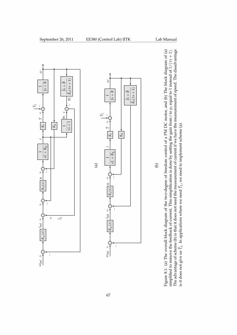
September 26, 2011 EE380 (Control Lab) IITK Lab Manualω
ref+
Kω(s)
i ref+
+K
I(s)
u+
1sL
+R
Σ
iK
tT
+
T L −1
Js+
Bω
Kb
−−
Js+
BK
t(τ
s+1)
1τ
s+1
y 1+
y 2−
i L+−
(a)
ωre
f+
Kω(s)
i ref+
KI(
s)u
+1
sL+
RΣ
iK
tT
+
T L −1
Js+
Bω
Kb
−
Js+
BK
t(τ
s+1)
−−
(b)
Figu
re8.
1:(a
)T
heov
eral
lbl
ock
diag
ram
ofth
etw
o-de
gree
offr
eedo
mco
ntro
lof
aPM
DC
mot
or,
and
(b)
The
bloc
kdi
agra
mof
(a)
sim
plifi
edto
rem
ove
the
feed
back
ofcu
rren
t.Th
issi
mpl
ifica
tion
isdo
neby
sett
ing
the
gain
from
ito
y 1eq
ualt
o1
inst
ead
of1/
(τs+
1).
The
adva
ntag
eof
sche
me
(b)i
sth
atit
does
notn
eed
the
mea
sure
men
tofc
urre
ntif
we
have
the
mea
sure
men
tofs
peed
.The
disa
dvan
tage
isit
does
notg
ive
usT L
.In
appl
icat
ions
whe
rew
ene
edT L
,we
need
toim
plem
ents
chem
e(a
).
67

September 26, 2011 EE380 (Control Lab) IITK Lab Manual
8.4 M-files
%% expt6.mclc; clear all; close all;format long
T = 0.002; tend = 2; t = 0:T:tend;La = 0.00077; % in HJm = 13.0e-7; % in kg m^2Jg = 0.4e-7; % in kg m^2Kt = 0.0255; % in Nm/AKb = 0.0255; % in V/(rad/sec)J = Jm+Jg;
%% practical values from step responseB = 5.41e-6;Ra = 31;
%% SimulationCi = 100; % inner controller (current controller)
% let speed controller Cw = (a1*s+a2)/(s+a3)b0 = 0.001157; b1 = 0.0222; a1 = 0.02218;Wr(1:tend/T+1) = 100;wf = 100; %% filter frequency in rad/sec
% TL = 0.00316; % for 2 Kg 0.01*9.8*2/62tTL = 1; % time when the TL is appliedTL(1: tTL/T) = 0;TL(tTL/T+1:tend/T+1) = 0.00316;
% InitializationW = 0; xw = 0; xid = 0; xir = 0;for k = 1:tend/T+1% Speed controllerew(k) = Wr(k) -W(k); % speed errorIref(k) = (b1-b0*a1)*xir(k) + b0*ew(k);xir(k+1) = (1-a1*T)*xir(k) + T*ew(k);
% estimation of Ihat = Im-ILIhat(k) = (B*wf/Kt - J*wf^2/Kt)*xw(k) + J*wf/Kt*W(k);xw(k+1) = (1-T*wf)*xw(k) + T*W(k);
% Inner controller (Current controller)u(k) = Ci*(Iref(k) - Ihat(k));
% motor speed calculationW(k+1) = ( 1 - B*T/J - Kt^2*T/Ra/J )*W(k) + Kt*T/J/Ra*u(k) -T/J*TL(k);end
68

September 26, 2011 EE380 (Control Lab) IITK Lab Manual
%% plot the responsesubplot(3,1,1), plot(t, TL); grid;title(’T_L [in Nm]’);subplot(3,1,2), plot(t, u); grid;title(’Controller output voltage [in V]’);subplot(3,1,3), plot(t,Wr, t,W(1:tend/T+1)), grid;title(’Speed \omega [in rad/sec]’); legend(’\omega_r’, ’\omega’)
69

September 26, 2011 EE380 (Control Lab) IITK Lab Manual
70

Chapter 9
Experiment 8: PMDC motormodeling, identification,position control
9.1 Goals
Modeling and identification (using OL step response) of PM DC motor. Designusing root locus and implementation of position controller for both. Compari-son of results.
9.2 Introduction
In this experiment we will study the theoretical and practical aspects of thecontrol of the angular displacement of the shaft of a PM DC motor using amicrocontroller. The block diagram of the setup is as shown in Figure 1.1. AdsPIC30F4012 micro-controller is used as the platform on which to implementour digital controller, and H-bridge four-quadrant DC chopper is used to drivethe DC servo motor. Please see the first two chapters of this manual for thedetails of the hardware and the software platform. Follows a list of questionsfor this experiment.
9.3 Mathematical model of DC servo motor
Since the inductance La is very small, we may neglect La. Then the TF betweenthe motor shaft position θ(s) and the armature voltage V(s) is
θ(s)V(s)
=Km
s(τms + 1)(9.1)
where, Km is the motor gain constant and τm is the motor time constant. Theseare as in Equation (2.1).
The parameters of the motor, gear, and encoder are provided in Table 1.1.
71

September 26, 2011 EE380 (Control Lab) IITK Lab Manual
9.4 Dead zone in the Vm versus u characteristic
The dead zone in the Vm versus u charaacteristic of Figure 1.6 did not affectmuch in the control of the speed of the DC motor as the speed was needed tobe at a large value and u quickly becomes large.
In the case of control of position of the shaft of the shaft of the DC mo-tor, however, u may become small when the desired position is reached. If ubecomes smaller than 2 volts when Vs = 12 V, then Vm will be zero, and theposition control system will become unresponsive. To overcome this situationwe have two alternatives:
1. Use an integral component in the controller.
2. Add the following code in main-prog.c before or after the if condition usedfor limiting the duty ratio.
if(u<0&&u>-2)u = u - 2;
else if(u>0&&u<2)u = u + 2;
9.5 Questions
9.5.1 To do at home
Q1 Determine the physics-based mathematical model of the DC servo motorwhose parameters may be found in the attached data sheets.
Q2 Design using root locus techniques a controller of at least first order andat most second order to control the angular displacement of the shaft of thegiven motor for the following time domain specifications: ess ≤ 2%, ts = 0.5s, Mp ≤ 20%.
For root locus-based design, please see the class notes from EE250_Fall2010.
Q3 Simulate the continuous-time controller designed above using Matlab.
If the closed-loop system performance in simulation is not as desired, youmay need to redesign your controller.
Q4 Discretize the continuous-time controller.
Q5 With the discretized version, perform a simulation of digital control of thecontinuous-time plant using the m-file provided in Experiment 1.
Do you think that your digitally-controlled closed-loop system will be stablein practice? Will it provide in practice the same performance as did thecontinous-time version in simulation?
Q6 Write the digital controller in C.
72

September 26, 2011 EE380 (Control Lab) IITK Lab Manual
9.5.2 To do in lab
Q7 Write a code to give a step input to the given motor. Run the setup in OLmode.
Q8 Identify the system parameters Km and τm by using the OL step response.
Q9 For the identified model, redesign your controller using root locus in MAT-LAB.
Q10 With the discretized version of the above-redesigned controller, performa simulation of digital control of the continuous-time plant using the m-fileprovided in Experiment 1.
Q10 Program the home-designed digital controller and run the setup. Recordand plot the necessary data.
Q11 Program the lab-designed digital controller and run the setup.
Q12 Compare the following results:
1. those using the controller designed for the physics-based model and ob-tained on Matlab,
2. those using the controller designed for the physics-based model and ob-tained from the experimental setup,
3. those using the controller designed for the identified model and obtainedon Matlab,
4. those using the controller designed for identified model and obtainedfrom the experimental setup.
Q13 Conclusions:
1. Is the physics-based model a good match to the plant? If not, what doyou think we have ignored that has lead to the difference?
2. What are the skills you learned from this experiment?3. Would you have preferred to learn a different skill set from the control
lab? If yes, which skills?4. How could we have organized this experiment differently to make it
more meaningful to you?
73

September 26, 2011 EE380 (Control Lab) IITK Lab Manual
74

Bibliography
[1] Frank L.Lewis and Vassilis L.Syrmos. Optimal Control, pages 67–68. WileyInterscience, 2 edition, 1995.
[2] Gene F. Franklin, J. David Powell, and Michael L. Workman. Digital Con-trol of Dynamic Systems. Addison-Wesley, 3 edition, 1998.
[3] Katsuhiko Ogata. Modern Control Engineering. Pearson Education, fourthedition, 2002. Available in India.
[4] Tore Hägglund and Karl J. Åström. Automatic tuning of PID controllers.In William S. Levine, editor, The Control Handbook, pages 817 – 826. CRCPress LLC, 1996.
[5] Gene F. Franklin, J. David Powell, and Abbas Emami-Naeini. FeedbackControl of Dynamic Systems. Pearson Education, fourth edition, 2002.
[6] Graham C. Goodwin, Stefan F. Graebe, and Mario E. Salgado. ControlSystem Design. Prentice-Hall, 2001. Published in India by Prentice-Hall ofIndia Pvt. Ltd.
[7] SGS-Thomson Microelectronics. TDA7274: Low-voltage dc motor speedcontroller, 1988. Data sheet.
[8] Wei Zhan. Sensorless speed control for dc permanent magnet motors.In Proceedings of the ninth IASTED International Conferene CONTROL ANDAPPLICATIONS, pages 116 – 120. 2007.
[9] Centent Company. CN0055 & CN0055B: dc to dc negative resistancespeed control, 2011. Datasheet.
[10] A. Cordeiro, D. Foito, and M. Guerriro. A sensorless speed control sys-tem for an electric vehicle without mechanical differential gear. In IEEEMELECON 2006, pages 1174 – 1177. Benalmadena, Malaga, Spain.
[11] Gopal K. Dubey. Fundamentals of electrical drives. Narosa, 2001.
[12] Maxon Motors. 5 years on mars. http://www.maxonmotor.com/media_releases_5619.html, 2009.
[13] Hamid A.A. Toliyat and Gerald B. Kliman, editors. Handbook of ElectricMotors, chapter Electronic Motors. CRC Press, second edition, 2004.
75

September 26, 2011 EE380 (Control Lab) IITK Lab Manual
[14] Takaji Umeno and Yoichi Hori. Robust speed control of dc servomotorsusing modern two degrees-of freedom controller design. IEEE Transactionson Industrial Electronics, 38(5):363 – 368, October 1991.
76

September 26, 2011 EE380 (Control Lab) IITK Lab Manual
77