Lab 4: Drainage Basin Morphometry Objectives: To better appreciate the usefulness of topographic maps as tools for investigating drainage basins and to master several morphometric variables used to characterize and analyze drainage basins.

This exercise is divided into the following sections: Section One: Introduction Section Two: A Few Fundamental Basin Parameters Section Three: Drainage Networks Section Four: Hypsometric Curves Section Five: Laboratory Exercise

Section One: Introduction

The fundamental unit of virtually all watershed and fluvial investigations is the drainage basin. An individual drainage basin (a.k.a. catchment or watershed) is a finite area whose runoff is channeled through a single outlet. In its simplest form, a drainage basin is an area that funnels all runoff to the mouth of a stream. Drainage basins may be delineated on a topographic map by tracing their perimeters or drainage divides. A drainage divide is simply a line on either side of which water flows to different streams. Locally, the most famous drainage divide is the Continental Divide. Each drainage basin is entirely enclosed by a drainage divide. Drainage basins are commonly treated as physical entities. For instance, flood control along a particular river invariably focuses on the drainage basin of that river alone. Because drainage basins are discrete landforms suitable for statistical, comparative, and analytical analyses, innumerable means of numerically and qualitatively describing them have been proposed. This laboratory is an introduction to some of the means by which drainage basins are described, particularly via drainage basin morphometry. Morphometry is essentially quantitative, involving numerical variables whose values may be recovered from topographic maps. The importance of morphometric variables is their usefulness for comparisons and statistical analyses.

Section Two: A Few Fundamental Basin Parameters

The simplest of drainage basin parameters are those that summarize spatial characteristics. Although such data are extremely important, the values do not lend themselves to detailed quantitative analysis of drainage basins; whether these values rise to the level morphometric variables is debatable. Spatial parameters prove valuable, however, in determining whether basins are sufficiently similar for direct comparison. For example, to study the effects of fire, one might compare a vegetated watershed with a burned watershed. For this comparison to isolate the effects of fire, other spatial factors (drainage area, relief, etc.) should remain relatively constant between drainage basins. In addition, spatial variables are used to calculate a wide variety of more sophisticated parameters. The procedures for determining a few fundamental

basin parameters are discussed in this section. However, before we consider these parameters we must first delineate the perimeter of the drainage basin of interest.

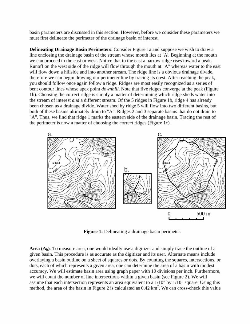
Delineating Drainage Basin Perimeters: Consider Figure 1a and suppose we wish to draw a line enclosing the drainage basin of the stream whose mouth lies at ‘A'. Beginning at the mouth we can proceed to the east or west. Notice that to the east a narrow ridge rises toward a peak. Runoff on the west side of the ridge will flow through the mouth at "A" whereas water to the east will flow down a hillside and into another stream. The ridge line is a obvious drainage divide, therefore we can begin drawing our perimeter line by tracing its crest. After reaching the peak, you should follow once again follow a ridge. Ridges are most easily recognized as a series of bent contour lines whose apex point downhill. Note that five ridges converge at the peak (Figure 1b). Choosing the correct ridge is simply a matter of determining which ridge sheds water into the stream of interest and a different stream. Of the 5 ridges in Figure 1b, ridge 4 has already been chosen as a drainage divide. Water shed by ridge 5 will flow into two different basins, but both of these basins ultimately drain to "A". Ridges 2 and 3 separate basins that do not drain to "A". Thus, we find that ridge 1 marks the eastern side of the drainage basin. Tracing the rest of the perimeter is now a matter of choosing the correct ridges (Figure 1c).

Figure 1: Delineating a drainage basin perimeter.

Area (Ab): To measure area, one would ideally use a digitizer and simply trace the outline of a given basin. This procedure is as accurate as the digitizer and its user. Alternate means include overlaying a basin outline on a sheet of squares or dots. By counting the squares, intersections, or dots, each of which represents a given area, one can determine the area of a basin with modest accuracy. We will estimate basin area using graph paper with 10 divisions per inch. Furthermore, we will count the number of line intersections within a given basin (see Figure 2). We will assume that each intersection represents an area equivalent to a 1/10" by 1/10" square. Using this method, the area of the basin in Figure 2 is calculated as 0.42 km2. We can cross-check this value

using a digitizing tablet. Doing so yields an area of 0.425 km2. The grid intersection method yielded a fair approximation of the area, but is entirely less satisfactory when areas are small relative to the fineness of the grid.

Figure 2: Measuring drainage basin area by counting grid intersections. In this case, each intersection would represent 10,000m2. The area of this basin is therefore 4,518,528ft2, 0.162mi2, 420,000m2, or 0.42km2. Can you recover these values yourself?

This exercise will use standard USGS topographic maps with a scale of 1:24000. Therefore, we must determine the area each 1/10" by 1/10" square would represent on a 1:24000 scale map. Recall from Lab One that 1 inch equals 2000 feet on a 1:24000 scale map. Given this information, you should now perform the calculations to determine how many square feet, miles, meters, and kilometers are represented by each 1/10" by 1/10" square on a 1:24000 map.

Relief/Height (H): As discussed in Lab One, relief is calculated by determining the difference between any two elevations. Relative to a drainage basin, relief is measured by subtracting the elevation of the mouth of the basin from the highest point within the basin. Some workers refer to this parameter as basin height. For this lab, you will interpolate the elevation of the basin mouth to the nearest 10 feet and perform the associated subtraction.

Perimeter Length (P): Perimeter length is the linear length of a drainage basin perimeter. One can measure this length with a string, map wheel, or digitizer. We will use a map wheel or digitizer. A map wheel is a pen-like device with a small wheel at the tip and large dial on top. By moving the wheel along a line an arm on the dial is moved. The length of the line, typically measured in inches, is read directly from the position of the arm on the dial. Converting the dial units into ground distance is a simple matter. For instance, if the wheel transcribed a distance of 2.5 inches on a 1:24000 scale map, one we can readily calculate that 2.5 inches multiplied by 2000 feet/inch equals 5000 feet. Hence, the line we measured represents a distance of 5000 feet on the ground.

Section Three: Drainage Networks and Morphometry Part One: Tracing Stream Paths Having established the outline, area, and relief of a basin, we are ready to consider the network of streams within the watershed. The importance of streams in quantitatively describing a drainage basin can not be overstated, as many morphometric variables are directly or indirectly calculated using stream lengths. However, when we examine stream networks an immediate problem arises. Specifically, one is always faced with the question, "What constitutes a stream?" Certainly a channel with perennial flow is a stream. But, toward the end of the drainage network streamflow is typically ephemeral; flow occurs only after precipitation or snow melt. Channels may be well defined, but are they streams? We will assume that all channels are streams. Stream length, or more appropriately channel length, is an important morphological variable. How do we quantify this variable in any given basin? For instance, one might utilize 7.5 minute topographic quadrangles to estimate stream length. Because streams incise, contours "V" across them. Hence, we can trace all the stream channels on a map by identifying "V's". After drawing lines through all the "V's" and connecting them together we have an approximation of the stream network. (Note that many of these streams will probably be ephemeral.) We can measure the length of the streams and thereby quantify stream lengths. Imagine performing the same task using a 1:250000 scale map. Because of the reduction in detail the stream network will appear shorter for a given basin. For a 1:10000 map, the stream density will probably be higher. So, map scale may play a direct role in determining stream lengths. A solution to the problem of map scale and resolution is to map channel lengths in the field. Such labor intensive work will undoubtably produce even greater stream lengths and will entail many difficult decisions. Once again one must be very careful about what constitutes a stream. Does every ascending gully, hollow, notch, or rill constitute a stream or only those that have definable channel banks? Clearly, stream length will vary from study to study, map to map, and investigator to investigator. For consistency, we will utilize an arbitrary set of rules for delineating streams and measuring their lengths. The rules are outlined below and are depicted in Figure 3. Assume that:

1. Contour lines that do not "V" or appear notched are not crossed by a stream (Figure 3a).

2. A stream can be traced through five or more successive contour lines with aligned "V's". Streams 1, 4, and 5 on Figure 3b.

3. A stream can be traced when two, three, or four successive contour lines possess aligned "V's" and are spaced more than 10% of a basins length apart. Streams 2 and 3 on Figure 3b.

4. Where "V's" are no longer found uphill of a notched contour line assume that the channel ends midway between the two contour lines.

Figure 3: Tracing stream paths on a topographic map. Notched contours are assumed to possess stream channels, unnotched contours are assumed to lack well-defined channels. Numbered streams are discussed in text.

Tracing stream paths on a topographic map is as much an art as a skill. Consistency, however, is extremely important. If you follow the rules your results should be readily comparable to other studies performed using the same procedure.

Part Two: Stream Order

Streams may be categorized according to their position--order or magnitude--within a drainage network. Stream order can be used to describe a stream and to conveniently divide a stream network into component parts that may be quantified and compared. For instance, streams that do not possess a tributary are designated as ‘1st order' or ‘magnitude 1' streams. The number and length of 1st order streams in a basin can be measured and compared to those in a separate basin. Such procedures lend themselves to statistical treatment and are therefore extremely useful for comparing different drainage basins. Two principal stream order schemes are in use today. The Strahler Order system designates 1st order streams as those that lack a tributary. Second order streams are formed at the junction of 1st order streams (Figure 4). Third order streams are formed at the junction of 2nd order streams, fourth at the junction of 3rd order streams, and so forth. Note that stream order only increases when two streams of the same order join. Therefore, where a 2nd order stream joins a 3rd stream there is no change in stream order; the 3rd order stream remains 3rd order. The Shreve Magnitude system designates streams that lack a tributary as magnitude 1. Where streams join, their magnitudes are added together. Therefore unlike the Strahler system, magnitudes increase at all junctions in the Shreve system. For instance, where a magnitude 2 stream joins a magnitude 3 stream, the magnitudes are added to form a magnitude 5 stream. Note that in such a case there is no magnitude 4 stream. A convenient component of the Shreve system is that a stream's magnitude corresponds to the number of magnitude 1 or 1st order streams contributing to the channel.

Figure 4: Stream order. Orders increase in the Strahler stream order system where two streams of equal order meet. In the Shreve magnitude system, magnitudes increase through addition at all stream junctions. Using the Shreve system, the number of magnitude 1 streams in a basin is equal to the basin's magnitude.

The number of 1st order streams in a basin of a given size is dependent upon a variety of climatic, geologic, and hydrologic factors. For instance, holding all other variables constant we would expect that a drainage basin in an arid climate would have more 1st order streams than a watershed in a more humid climate. Similarly, increasing relief is associated with increasing stream densities. Although the number of streams in a given order is a crude measure of drainage density, we define drainage density (D) much more explicitly as,

where Li denotes stream lengths and Ab is drainage basin area

Measuring stream lengths is accomplished using a map wheel or digitizing table. During this exercise, we will measure the length of all streams in each order. Drainage density will be calculated by summing the lengths of all orders and dividing by basin area. Prior to measuring the stream lengths you should pause and predict which stream order will have the greatest length. Why is this relationship important?

Not only are the numbers and lengths of particular stream orders important, but their ratios are quite instructive as well. Consider a dendritic drainage pattern versus trellis. In an ideal dendritic drainage pattern, the number of 1st order tributaries would be exactly twice the number of 2nd order streams. Thus, the number of 1st order streams will be exactly twice that of 2nd order streams. In a trellis network, long main stem streams are fed by many low order streams. As a result, 1st order streams typically outnumber 2nd order streams by 3 to 5 times. The relationship

between the number of streams in successive stream orders is called the bifurcation ratio (Rb). The ratio can be mathematically defined as follows,

where So is the number of streams in any given order and So-1 is the number of streams in the next lowest order.

For Figure 4a, note that the bifurcation ratio between the 1st and 2nd order streams can be computed as follows,

The utility of the bifurcation ratio lies in its ability to succinctly express the organization of a drainage basin and allow statistical tests. As a mental exercise, you might consider two streams with similar areas, relief, and so forth. Their drainage patterns differ with one possessing a 1st/2nd bifurcation ratio of 2.4 and a 2nd/3rd ratio of 2.2. The other stream possesses values of 4.7 and 4.1. Using logic, can you accurately predict which watershed has the flashiest hydrograph at its mouth? The solution is, perhaps, more complex than it appears. Part Three: More Drainage Basin Morphometry Variables Having familiarized ourselves with the techniques used to delineate drainage basins and drainage networks, as well as a few techniques with which to characterize them, we can now begin to quantitatively describe drainage basins in some detail. The following are variables commonly used in morphometric analysis. Basin Shape (Rf): A measure of the elongation of a basin. As elongation increases for a given area, Rf decreases (see Figure 5). For instance, a circular basin with an area of 3.14 mi2 would have an Rf value of 3.14. Whereas an elliptical basin 1.5 miles long, but with an area of 3.14 mi2 would have an Rf value of 1.4.

Figure 5: Basin shape. For a given area, as basin length increases the value Rf decreases.

The value Rf should be comparable among basins of very different size. To calculate Rf, simply measure the linear distance (L) between the mouth of the basin and the point most distant from the mouth and use the formula:

Ruggedness number (R): A combined measure of relief and stream density. As topography becomes more convoluted, the ruggedness number increases. To calculate R, multiply the drainage density (D) by basin relief (H). Be sure to use the same unit of length as used in calculating drainage density (typically kilometers),

R = DH Relief Ratio (Rh): A unitless measure of the overall gradient across a basin. Calculated by dividing the relief (H) of a basin by its length (L). Be sure to use values with equal units,

Section Four: Hypsometric Curves Part One: Creating Hypsometric Curves Landforms are classified, in large part, by their geometry. For instance, the term mesa immediately conjures images of a table-like hill or mountain. Quantitative or qualitative description of drainage basins is more difficult. Although drainage networks may be classified according to the geometry of their branches and quantitatively described by orders, lengths, areas, and densities we are still faced with the problem of describing the distribution of basin area relative to height.

As an example, basin relief measures only the difference between the highest and lowest points in a watershed. As a result, a stream draining a high plateau and plunging into a gorge might have the same relief as the drainage basin around Devil's Tower, Wyoming. Clearly, the two watersheds have different distributions of land. One has the vast majority of its area higher in the basin and the other (Devil's Tower) has only a small amount of its land higher in the basin. How can we quantitatively compare these very different drainage basins? As one might anticipate from the title of this section, the answer is hypsometric curves. Strahler first introduced hypsometric curves--his method survives unchanged. To understand hypsometric curves we will do an example using the example basin Figure 4. We begin by recalling that basin relief and area are, respectfully, 654 feet and 0.425 km2. Recall also that the contour interval is 40 feet. Using these values, the procedure is as follows:

1. Divide the elevation range of the basin into elevation class intervals. Begin by dividing the relief by multiples of the contour interval until the resulting value is near a whole number. Our goal is to arrive at class intervals that can be traced by following contours on the map. A lit tle calculation shows that we can divide 654 by 80 feet to arrive at a value of 8.125. Thus, we can start at the bottom of the drainage basin and trace class boundaries at every second contour line (80 feet; Figure 6). In doing so, we will divide the drainage basin into 9 elevation class intervals. These intervals are listed in Table 1.

Figure 6: Division of basin into elevation class intervals. Intervals are 80 feet wide. Shading the classes reveals that the majority of basin area lies at comparatively high relief.

2. Measure the area of the basin above the bottom of each elevation class interval. For instance, using graph paper or a digitizer, measure the area of the basin that lies above the

8240 contour line. This represents the area of our last elevation class. Then measure the area of the basin above the 8160 contour line. Note that this includes the area of the eighth and ninth elevation class intervals. Continue this process with all of the elevation classes. Note that for the first interval, the area will be the same as the total basin area.

3. Determine the area proportion. Calculate the area proportion of the area above the bottom of each interval by dividing the area obtained in step 2 by the total drainage basin area.

4. Determine the relief above a given elevation class interval. For each elevation class interval, subtract the basin mouth elevation from the bottom class elevation. Notice that for the first elevation class, the resultant value will be zero.

5. Determine the fraction of relief that lies below the bottom of each interval. For each elevation class interval, divide the value obtained in Step 3 by the relief of the basin. This will provide the fraction of basin relief below the base of each elevation class interval.

6. Plot area proportion (x) versus height proportion (y). Notice that when the area proportion is highest, height proportion is lowest.

Elevation Interval

Area above bottom

of Interval (a)1

Area Proportiona/Ab

Lower Interval Elev.

- mouth elev. (h)

Height Proportion

(h/H)

7600-7680 0.425 km2 0.425 km2/0.425 km2 = 1 7600-7600 = 0 0/654 = 0.00

7680-7760 0.416 0.98 7680-7600 =80 0.122 7760-7840 0.392 0.92 160 0.245 7840-7920 0.343 0.81 240 0.367 7920-8000 0.271 0.64 320 0.489 8000-8080 0.183 0.43 400 0.612 8080-8160 0.141 0.33 480 0.734 8160-8240 0.088 0.21 560 0.856 8240-8320 0.012 0.03 640 0.979

1 Measured using a digitizing tablet.

Part Two: Interpreting Hypsometric Curves

Having constructed a hypsometric curve, we are left to ponder its meaning. As stated before, hypsometric curves graphically depict the distribution of basin area relative to height. Consider our calculations in a qualitative sense. Beginning at the mouth of a basin, area is at a maximum and relief is at a minimum. As you move upward in a basin, from the mouth, relief increases, but area decreases. So, if the majority of basin area lies at low elevations the area proportion will decrease more quickly than the height proportion. This will produce a concave hypsometric curve as seen in Figure 7a. However, if the majority of basin area lies at high elevations the height proportion will decrease more quickly than the area proportion. This will produce a convex hypsometric curve as seen in Figure 7b.

Consider the basins draining the plateau and the area around Devil's Tower, Wyoming. As one moves ‘up-basin' from the mouth of the basin draining the plateau, relief is quickly gained as one climbs out of the gorge. But, area will decrease much more slowly because more of the basin lies atop the plateau. Simply put, the majority of basin area lies at high elevations, but the majority of relief is gained low in the basin. This will produce a convex hypsometric curve (Figure 7b). In the case of Devil's Tower, area is gained quickly as one moves ‘up-basin', but relief only increase dramatically when one reaches the tower. Because the tower represents very little area compared to its contribution to relief we would find that it possesses the greatest proportion of relief for a very small proportion of area. Thus, the hypsometric curve will be sharply concave (Figure 7a).

Figure 7: Examples of hypsometric curves. Concave form of (a) indicates that the majority of basin area lies at comparatively low relief. Convex form of (b) indicates that the majority of basin area lies at comparatively high relief. Typically, (a) would be associated with a dissected, eroded landscape while (b) would be associated with more youthful terrain with deeply incised, narrow valleys and broad upland areas.

The usefulness of hypsometric curves becomes evident at this point. Imagine a large geologically young plateau. The plateau will be dissected by numerous gorges and thus possess high relief, but most of the area will lie high in the basin. Hypsometric curves of watersheds draining the plateau will be convex. As the plateau is gradually eroded, the uplands will be eroded and valleys will widen. As this happens, the area of the basin at low relief (valleys) increases while the area of the basin at high relief decreases (mountains or plateau surfaces). Thus, with time the hypsometric curve will be concave. Therefore, we can compare hypsometric curves from different watersheds and indirectly arrive at conclusions about more than their distribution of area relative to relief. We can compare evolution of the landscapes and directly compare degrees of dissection (assuming the basins all began with a similar distribution of area versus relief). Such comparisons are all the easier given that hypsometric proportions are unitless and possess values between zero and one.

Section Five: Laboratory Exercise

The following exercise focuses on quantitative drainage basin characterization and analysis. Given that the ultimate goal of drainage basin analysis is to understand the underlying geomorphologic processes, the exercise is designed as a two part, group exercise. Each person will characterize a drainage basin using the techniques outlined previously. The four basins are drawn from three states (Colorado, Virginia, and North Carolina) and one of the four has already been characterized for you. Each basin possesses distinctive topography and drainage basin parameter values. Thus, the four can be compared and inferences can be made about the different processes acting to shape each basin. For instance, the North Carolina watershed receives nearly 4 times the amount of precipitation as the Colorado basin. We can quantitatively explore how differences in this parameter and others is this expressed in the nature of the basins.

Assignment: Perform the following tasks.

1. Form a group of three people. Assign one of the three basins to each person. 2. Each person should complete the two worksheets for their basin. The worksheets area

labeled: Hypsometric Curve Worksheet (see below) Drainage Basin Morphometry Worksheet (see below)

3. Compile the completed worksheets. (Thus each group will turn in 3 hypsometric curve worksheets and one composite drainage basin morphomotry worksheet)

4. Interpret the amassed data and write a 1-2 page group paper that quantitatively and qualitatively compares the four basins. In the group report, be sure to suggest explanations for why the basins possess different values for the various drainage basin parameters and to interpret the hypsometric curves. Why do the three hypsometric curves generated by your group appear so different? Does this suggest different landscape ages or erosion processes? Consult your lecture text for help with the report. Along with your paper you will turn in your worksheets, and the basin tracings from each group member.

Hypsometric Curve Worksheet

Elevation Interval

Area above bottom

of Interval (a)1

Area Proportion

a/Ab

Lower Interval Elev

-mouth elev (h)

Height Proportion

(h/H)- . . . . - . . . . - . . . . - . . . . - . . . . - . . . . - . . . . - . . . . - . . . . - . . . . - . . . . - . . . . - . . . . - . . . .

To generate a hypsometric curve from the data above, plot the area proportion (x) versus height proportion (y) using a spreadsheet in Excel.

Drainage Basin Morphometry Worksheet

Basin

Variable Colorado

Front Range(Poudre)

ColoradoRockies

(Mt Evans)

North Carolina (Luftee)

Virginia (Swift Run)

Climate Semi-arid,alpine

Semi-arid,sub-arctic

Humid, temperate

Humid, temperate

Average Yearly Precipitation (cm) 38 89 120 115 Vegetation Scrub/Pine Tundra/Pine Hardwood Hardwood Bedrock Metamorphic Granite Granite Meta./GraniteArea (km2) . 3.9 . . Relief (m) . 596 . . Perimeter Length (km) . 4.27 . . Gradient (longest path) . 0.105 . . Relief Ratio . 0.154 . . Drainage Pattern (name) . Dendritic . . Number of 1st Order Streams . 12 . . Number of 2nd Order Streams . 3 . . Number of 3rd Order Streams . 1 . . Number of 4th Order Streams . - . . Order of Master Stream (Shreve) . 12 . . Order of Master Stream (Strahler) . 3 . . Length of 1st Order Streams (km) . 5.95 . . Length of 2nd Order Streams (km) . 1.68 . . Length of 3rd Order Streams (km) . 1.37 . . Length of 4th Order Streams (km) . - . . 2nd Order Bifurcation Ratio (No1st/No2nd) . 4 . .

3rd Order Bifurcation Ratio (No2nd/No3rd) . 3 . .

4th Order Bifurcation Ratio (No3rd/No4th) . - . .

Sum of Stream Lengths (km) . 9.00 . . Drainage Density (km/km2) . 2.3 . . Ruggedness . 1.38 . .