Lab 1

Introduction to MATLAB xPC Toolbox and the Advantec PC 104 computer boards

Introduction

The PC104 standard is for a system of computers that are small in size, and stackable so that any

peripheral module with the same standard of size and number of pins can be interfaced to it. The systems

we will be using in the lab are made by Advantech. We have two different modules, the older PCM 3350

and the new PCM 3355L boards. They require low power and can be used for general purpose embedded

applications. You may read more about their specifications on their respective manuals uploaded on

blackboard.

In the lab each group will have access to two PC104 computers. They are installed with Diamond MM

A/D D/A boards and screw terminals that provide connections to them. In the first lab you will be

familiarizing yourselves with the various functionalities/capabilities of these embedded computer

systems. You will also learn how to use the MATLAB xPC Target toolbox for embedded systems

programming. For all experiments performed in this lab, we will design models in Simulink and then

utilize a C compiler to create executable code from the models. The code will then be ported to the flash

memory on the PC104 board and run from there.

By the end of this lab, you should be well informed and completely comfortable in utilizing the various

resources these PC104 systems have to offer. All the skills you learn in this lab will be required in future

labs for successful completion of the semester.

NOTE: The computer systems in GWC laboratory are such that they lose all information upon restart and

also at 12:00 am midnight. As such, it is strongly recommended to carry flash drives and save all your

work in it at all times. Also, MATLAB needs to be configured in a particular manner for use in this lab.

Since the computers reset, these configurations will have to be done every time you come in.

Setting up Matlab for first use

These procedures must be followed every time you come to the lab.

Step 1. Compiler configuration

NOTE: Throughout these lab manuals, type command or run command means you should enter the

command into the MATLAB main command window. MATLAB always has “>>” symbol to indicate

where your commands are entered. We use the same symbol in this manual to indicate it is a MATLAB

command. To see what licenses and toolboxes are installed in MATLAB you can type “ver” and hit enter.

At the very bottom you should see the xPC Target and xPC Target Embedded Option listed. Without

them you cannot do any work related to this lab.

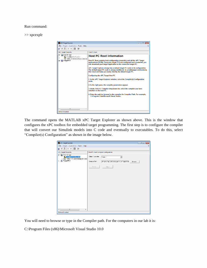
Run command:

>> xpcexplr

The command opens the MATLAB xPC Target Explorer as shown above. This is the window that

configures the xPC toolbox for embedded target programming. The first step is to configure the compiler

that will convert our Simulink models into C code and eventually to executables. To do this, select

“Compiler(s) Configuration” as shown in the image below.

You will need to browse or type in the Compiler path. For the computers in our lab it is:

C:\Program Files (x86)\Microsoft Visual Studio 10.0

Make sure you click “Apply” every time, after making any changes. If you move to a different window

without clicking “Apply”, the changes are not saved.

Step 2. Target PC configuration

xPC Explorer identifies each PC104 system as a target PC. By default the explorer will start with one

target named TargetPC1. Each target PC can be programmed to run in either “Standalone” mode or in

“DOS Loader” mode. We will look at each mode, their uses and how to configure them.

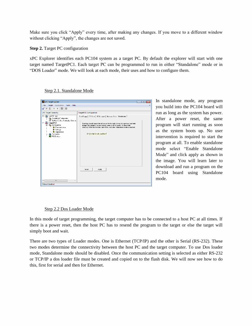
Step 2.1. Standalone Mode

In standalone mode, any program

you build into the PC104 board will

run as long as the system has power.

After a power reset, the same

program will start running as soon

as the system boots up. No user

intervention is required to start the

program at all. To enable standalone

mode select “Enable Standalone

Mode” and click apply as shown in

the image. You will learn later to

download and run a program on the

PC104 board using Standalone

mode.

Step 2.2 Dos Loader Mode

In this mode of target programming, the target computer has to be connected to a host PC at all times. If

there is a power reset, then the host PC has to resend the program to the target or else the target will

simply boot and wait.

There are two types of Loader modes. One is Ethernet (TCP/IP) and the other is Serial (RS-232). These

two modes determine the connectivity between the host PC and the target computer. To use Dos loader

mode, Standalone mode should be disabled. Once the communication setting is selected as either RS-232

or TCP/IP a dos loader file must be created and copied on to the flash disk. We will now see how to do

this, first for serial and then for Ethernet.

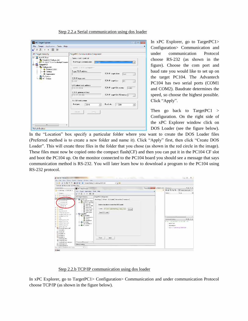
Step 2.2.a Serial communication using dos loader

In xPC Explorer, go to TargetPC1>

Configuration> Communication and

under communication Protocol

choose RS-232 (as shown in the

figure). Choose the com port and

baud rate you would like to set up on

the target PC104. The Advantech

PC104 has two serial ports (COM1

and COM2). Baudrate determines the

speed, so choose the highest possible.

Click “Apply”.

Then go back to TargetPC1 >

Configuration. On the right side of

the xPC Explorer window click on

DOS Loader (see the figure below).

In the “Location” box specify a particular folder where you want to create the DOS Loader files

(Preferred method is to create a new folder and name it). Click “Apply” first, then click “Create DOS

Loader”. This will create three files in the folder that you chose (as shown in the red circle in the image).

These files must now be copied onto the compact flash(CF) and then you can put it in the PC104 CF slot

and boot the PC104 up. On the monitor connected to the PC104 board you should see a message that says

communication method is RS-232. You will later learn how to download a program to the PC104 using

RS-232 protocol.

Step 2.2.b TCP/IP communication using dos loader

In xPC Explorer, go to TargetPC1> Configuration> Communication and under communication Protocol

choose TCP/IP (as shown in the figure below).

TCP/IP uses IPv4 addressing schemes to communicate with different Ethernet devices. We will not go

into a discussion about IPv4 addressing but enough to setup communications between the PC104 boards

and the host computer. These are the following options to configure:

Target PC IP address : the IP address labeled next to the PC104 board you are using (e.g 129.219.24.223)

TCP/IP target port : 22222

LAN subnet mask address : 255.255.255.192

TCP/IP gateway address : 129.219.24.193

Leave everything else as default. Click “Apply”.

To create a DOS Loader with Ethernet go back to TargetPC1 > Configuration. On the right side of the

xPC Explorer window click on DOS Loader (see the figure below). In the “Location” box specify a

particular folder where you want to create the DOS Loader files. Click “Apply” first, and then click

“Create DOS Loader”. This will create three files in the folder. These files must now be copied onto the

compact flash(CF) and the CF card inserted into the PC104 CF slot and boot the PC104 up. On the

monitor connected to the PC104 board you should see a message that says communication method is

TCP/IP and it will specify the IPv4 address, subnet mask and gateway you specified. You will later learn

how to download a program to the PC104 using TCP/IP protocol.

Step 2.3 Enabling secondary IDE

Go to xPC Explorer, under TargetPC1> Configuration> Settings and enable “Enable Secondary IDE” (see

figure above). This will allow you to store data on the CF card. This data can be anything starting from

error messages, A/D readings, serial port inputs etc.

Step 3 Model file Configuration

This needs to be done for every real time model you build. However unlike the setup processes in step 1

and step 2, these configurations are local to individual files. Since, the model files will be saved (not on

the lab computers); these configurations will not require redoing every time unless you specifically want

to change them.

Go to MATLAB main window, then click on File> New> Model

A new Simulink model file will appear. Then go to Simulink> Configuration Parameters as shown above.

In the window that appears set “Fixed step size” based on the lowest sample time you want to use on your

model (see figure below).

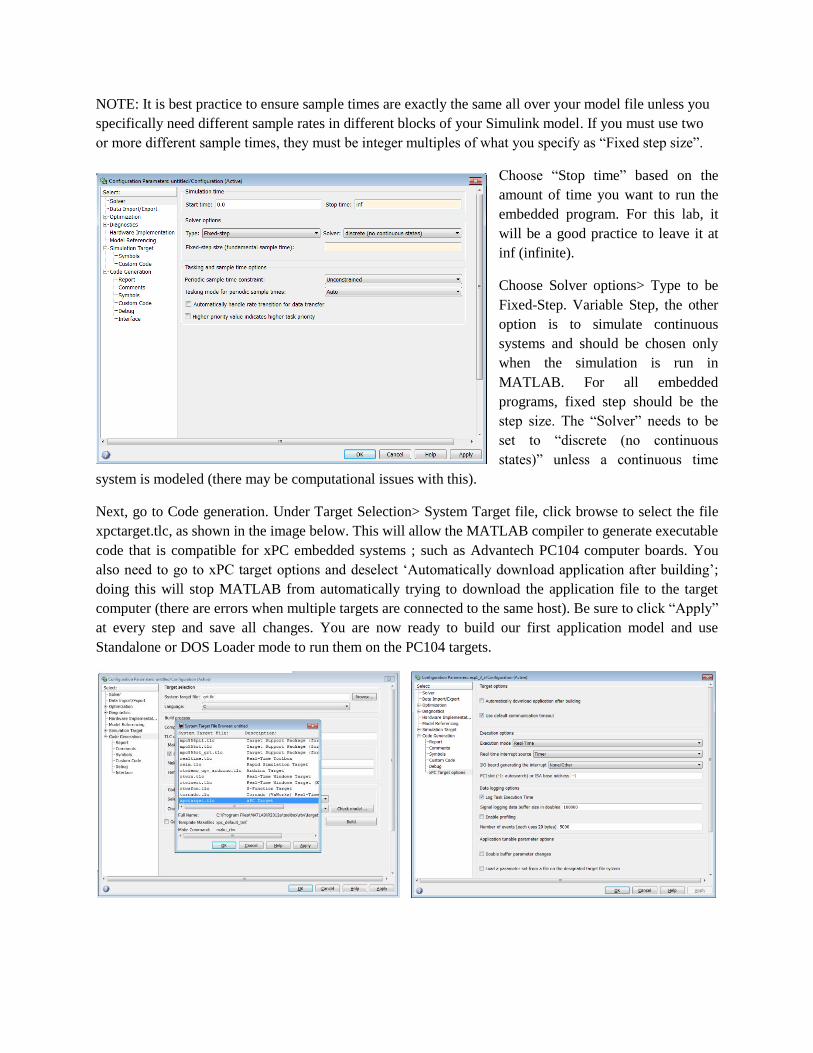
NOTE: It is best practice to ensure sample times are exactly the same all over your model file unless you

specifically need different sample rates in different blocks of your Simulink model. If you must use two

or more different sample times, they must be integer multiples of what you specify as “Fixed step size”.

Choose “Stop time” based on the

amount of time you want to run the

embedded program. For this lab, it

will be a good practice to leave it at

inf (infinite).

Choose Solver options> Type to be

Fixed-Step. Variable Step, the other

option is to simulate continuous

systems and should be chosen only

when the simulation is run in

MATLAB. For all embedded

programs, fixed step should be the

step size. The “Solver” needs to be

set to “discrete (no continuous

states)” unless a continuous time

system is modeled (there may be computational issues with this).

Next, go to Code generation. Under Target Selection> System Target file, click browse to select the file

xpctarget.tlc, as shown in the image below. This will allow the MATLAB compiler to generate executable

code that is compatible for xPC embedded systems ; such as Advantech PC104 computer boards. You

also need to go to xPC target options and deselect ‘Automatically download application after building’;

doing this will stop MATLAB from automatically trying to download the application file to the target

computer (there are errors when multiple targets are connected to the same host). Be sure to click “Apply”

at every step and save all changes. You are now ready to build our first application model and use

Standalone or DOS Loader mode to run them on the PC104 targets.

Experiment 1.1

Building familiarity with xPC toolbox and executing real-time code in PC104.

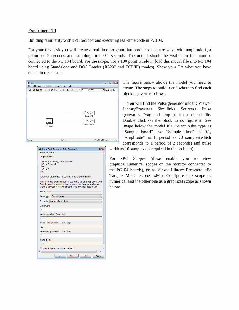
For your first task you will create a real-time program that produces a square wave with amplitude 1, a

period of 2 seconds and sampling time 0.1 seconds. The output should be visible on the monitor

connected to the PC 104 board. For the scope, use a 100 point window (load this model file into PC 104

board using Standalone and DOS Loader (RS232 and TCP/IP) modes). Show your TA what you have

done after each step.

The figure below shows the model you need to

create. The steps to build it and where to find each

block is given as follows.

You will find the Pulse generator under : View>

LibraryBrowser> Simulink> Sources> Pulse

generator. Drag and drop it in the model file.

Double click on the block to configure it. See

image below the model file. Select pulse type as

“Sample based”. Set “Sample time” as 0.1,

“Amplitude” as 1, period as 20 samples(which

corresponds to a period of 2 seconds) and pulse

width as 10 samples (as required in the problem).

For xPC Scopes (these enable you to view

graphical/numerical scopes on the monitor connected to

the PC104 boards), go to View> Library Browser> xPc

Target> Misc> Scope (xPC). Configure one scope as

numerical and the other one as a graphical scope as shown

below.

Once the model file is ready, save it and press Ctrl+b to build it. Then copy the three files shown in the

below figure into the flash disc.

NOTE: The “Current Folder” tab in the

MATLAB file explorer shows the active

working directory of MATLAB. You must

save all your model files in this folder or

else MATLAB will not know where the

file or its dependencies are. In the example

below ExpMdl is the active folder. So the

model was saved under it and when a build

was performed, all necessary files for

creating executables from C code were

created there. The executables are always

saved under the modelname_xpc_emb

folder. You must copy all these files and

put them into the CF card for your program

to run in Standalone Mode.

Experiment 1.2

Implement the same model used in exp 1.1 with a sample time of 0.01s, but this time use serial

communication to download the file onto the PC104 board.

To do this you need to connect a serial cable (DB-9) from the back of the host computer running

MATLAB to one of the two RS-232 ports on the PC104. The image below shows all the connectors you

will find on the PC104 board. See step 2.2.a to create DOS Loader files.

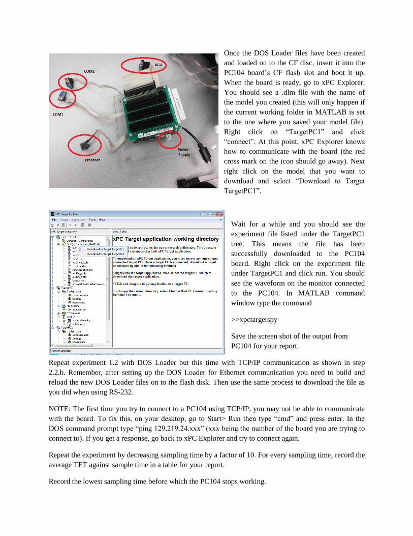
Once the DOS Loader files have been created

and loaded on to the CF disc, insert it into the

PC104 board’s CF flash slot and boot it up.

When the board is ready, go to xPC Explorer.

You should see a .dlm file with the name of

the model you created (this will only happen if

the current working folder in MATLAB is set

to the one where you saved your model file).

Right click on “TargetPC1” and click

“connect”. At this point, xPC Explorer knows

how to communicate with the board (the red

cross mark on the icon should go away). Next

right click on the model that you want to

download and select “Download to Target

TargetPC1”.

Wait for a while and you should see the

experiment file listed under the TargetPC1

tree. This means the file has been

successfully downloaded to the PC104

board. Right click on the experiment file

under TargetPC1 and click run. You should

see the waveform on the monitor connected

to the PC104. In MATLAB command

window type the command

>>xpctargetspy

Save the screen shot of the output from

PC104 for your report.

Repeat experiment 1.2 with DOS Loader but this time with TCP/IP communication as shown in step

2.2.b. Remember, after setting up the DOS Loader for Ethernet communication you need to build and

reload the new DOS Loader files on to the flash disk. Then use the same process to download the file as

you did when using RS-232.

NOTE: The first time you try to connect to a PC104 using TCP/IP, you may not be able to communicate

with the board. To fix this, on your desktop, go to Start> Run then type “cmd” and press enter. In the

DOS command prompt type “ping 129.219.24.xxx” (xxx being the number of the board you are trying to

connect to). If you get a response, go back to xPC Explorer and try to connect again.

Repeat the experiment by decreasing sampling time by a factor of 10. For every sampling time, record the

average TET against sample time in a table for your report.

Record the lowest sampling time before which the PC104 stops working.

Answer the following questions in your report.

Q1. Describe briefly the capabilities of the PC104 board and the Diamond MM A/D, D/A board with

mention about its important technical specifications like Processor, A/D range resolutions, serial

communication etc. and its application in not more than 150 words.

Q2. Give 5 examples of the practical applications where you can put PC104 boards to use?

Q3. What complier did you use to create a standalone to run on PC104?

Q4. Report the all the sample times you used on the board and average Execution Time of your program

before it stopped working.

Q5. What does the command xpctargetspy do?

Experiment 1.3

Generate the same pulse wave as you did in exp 1.1 and transmit it from one board then receive the same

signal on a second PC104 board. This transmission will be done over the serial ports of the PC104. Use

TCP/IP DOS Loader for all your work. Sample for this experiment will be 0.1s.

For this experiment you need to create a new target PC to utilize the second PC 104 board on your

system. To do this right click on Host PC Root and click on Add Target as shown below

You should now see a new target PC

named TargetPC2. For the new target

PC configure TCP/IP settings as given

on the second board. Create the DOS

Loader, copy the files on to the second

compact flash and boot the new PC104

up. Right click on the new Target PC

and click connect to ensure connectivity

to the new board.

For your experiment, create two new

model files as shown below.

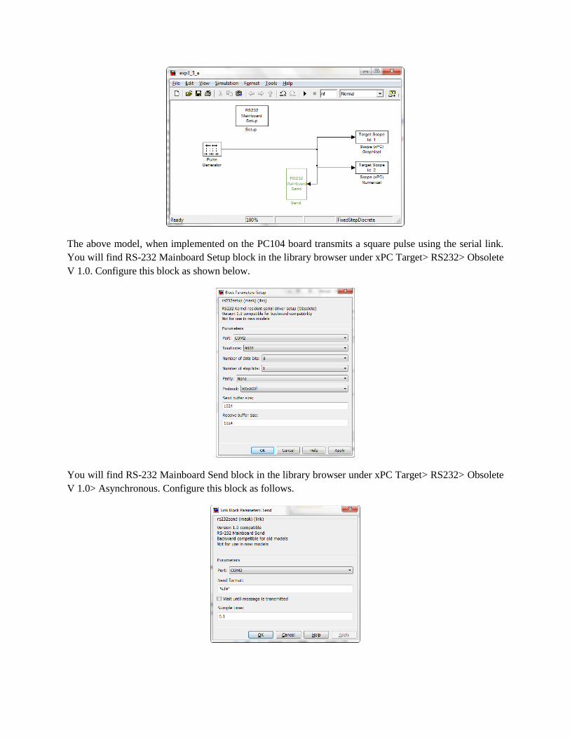
The above model, when implemented on the PC104 board transmits a square pulse using the serial link.

You will find RS-232 Mainboard Setup block in the library browser under xPC Target> RS232> Obsolete

V 1.0. Configure this block as shown below.

You will find RS-232 Mainboard Send block in the library browser under xPC Target> RS232> Obsolete

V 1.0> Asynchronous. Configure this block as follows.

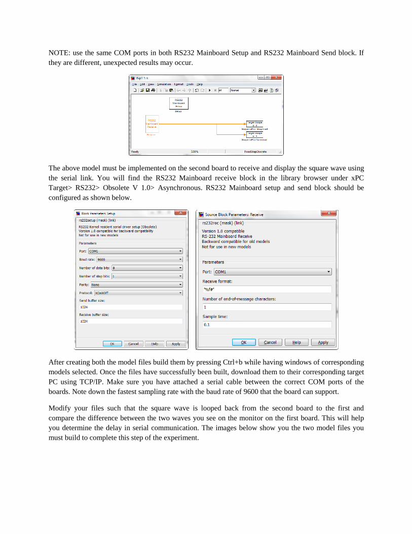
NOTE: use the same COM ports in both RS232 Mainboard Setup and RS232 Mainboard Send block. If

they are different, unexpected results may occur.

The above model must be implemented on the second board to receive and display the square wave using

the serial link. You will find the RS232 Mainboard receive block in the library browser under xPC

Target> RS232> Obsolete V 1.0> Asynchronous. RS232 Mainboard setup and send block should be

configured as shown below.

After creating both the model files build them by pressing Ctrl+b while having windows of corresponding

models selected. Once the files have successfully been built, download them to their corresponding target

PC using TCP/IP. Make sure you have attached a serial cable between the correct COM ports of the

boards. Note down the fastest sampling rate with the baud rate of 9600 that the board can support.

Modify your files such that the square wave is looped back from the second board to the first and

compare the difference between the two waves you see on the monitor on the first board. This will help

you determine the delay in serial communication. The images below show you the two model files you

must build to complete this step of the experiment.

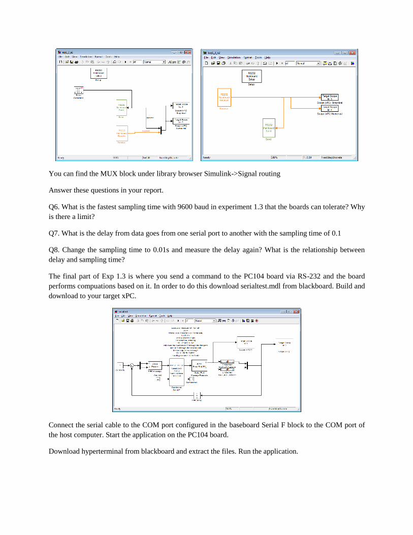
You can find the MUX block under library browser Simulink->Signal routing

Answer these questions in your report.

Q6. What is the fastest sampling time with 9600 baud in experiment 1.3 that the boards can tolerate? Why

is there a limit?

Q7. What is the delay from data goes from one serial port to another with the sampling time of 0.1

Q8. Change the sampling time to 0.01s and measure the delay again? What is the relationship between

delay and sampling time?

The final part of Exp 1.3 is where you send a command to the PC104 board via RS-232 and the board

performs compuations based on it. In order to do this download serialtest.mdl from blackboard. Build and

download to your target xPC.

Connect the serial cable to the COM port configured in the baseboard Serial F block to the COM port of

the host computer. Start the application on the PC104 board.

Download hyperterminal from blackboard and extract the files. Run the application.

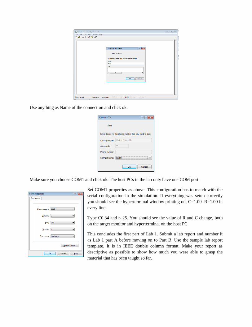
Use anything as Name of the connection and click ok.

Make sure you choose COM1 and click ok. The host PCs in the lab only have one COM port.

Set COM1 properties as above. This configuration has to match with the

serial configuration in the simulation. If everything was setup correctly

you should see the hyperterminal window printing out C=1.00 R=1.00 in

every line.

Type C0.34 and r-.25. You should see the value of R and C change, both

on the target monitor and hyperterminal on the host PC.

This concludes the first part of Lab 1. Submit a lab report and number it

as Lab 1 part A before moving on to Part B. Use the sample lab report

template. It is in IEEE double column format. Make your report as

descriptive as possible to show how much you were able to grasp the

material that has been taught so far.

This is Part B of Lab 1. You will need to submit a separate report for this section.

Experiment 1.4

Getting familiar with Diamond MM A/D and D/A boards.

Before building any blocks we need to get familiar with the diamond MM board and its functionalities.

The Diamond MM boards are a

multifunction analog and digital I/O

module compatible with the PC104

standard. It offers 16 single-ended or 8-

differential, bipolar analog inputs (A/D)

with 12 bit resolution. It has 2 analog

outputs (D/A) with 12-bit resolution,

however the D/A is a unipolar peripheral.

The board also features 8 digital inputs

and 8 digital outputs. Maximum sampling

rate that can be achieved using MATLAB

programming is 2 KHz, however with

DMA operation (cannot be done in

MATLAB) 100 KHz sampling rate can be

achieved. The image to the left shows how

the board will look once you take off the

screw terminal on top of it. It is important to read the jumper (J4, J5, J6 etc.) locations based on what is

top, left and right for the board as shown in the image. The Diamond MM manual is available in

Blackboard and is needed to learn how to configure the board for proper use. Make sure jumpers are at

the right position based on the configuration you want, follow instructions from diamond MM manual.

Build and compile the two model files as shown below.

You can find the MM Diamond analog Input block under Simulink library Browser> A/D> Diamond->

MM and the Diamond MM analog Output under Simulink library Browser> D/A> Diamond> MM

Configure A/D and D/A as follows

This experiment, as you see is similar to exp 1.3; although, here you are using the D/A and A/D modules

to transmit and receive the signal. Remember, that the D/A cannot transmit negative voltages. Connect the

ports you configured in the blocks with their corresponding pins on the screw terminal using wires

supplied to you in the lab. You should be able to see the waveform on the monitor.

In the second part of this experiment, you will determine the delay in A/D conversion. To do this, modify

your model files as shown below.

You may use the xpctargetspy command on the board running exp1_4_a2 then measure the difference in

the transmitted and looped back signal. The delay in one side of the conversion is then half of what you

measured off the screen.

Now, you will learn how to log and save data, this can be any signal, on to the flash disc. Add a new

target scope to the output of your exp1_4_a2 mux (multiplexer). Configure it as shown below. This

method configures the scope as a file scope. It saves the data in a file by the name specified in the

“Filename” box. Build and run your model and follow the next procedures to have the data transferred to

MATLAB workspace.

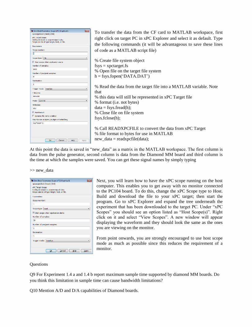
To transfer the data from the CF card to MATLAB workspace, first

right click on target PC in xPC Explorer and select it as default. Type

the following commands (it will be advantageous to save these lines

of code as a MATLAB script file)

% Create file system object

fsys = xpctarget.fs

% Open file on the target file system

h = fsys.fopen(‘DATA.DAT’)

% Read the data from the target file into a MATLAB variable. Note

that

% this data will still be represented in xPC Target file

% format (i.e. not bytes)

data = fsys.fread(h);

% Close file on file system

fsys.fclose(h);

% Call READXPCFILE to convert the data from xPC Target

% file format to bytes for use in MATLAB

new_data = readxpcfile(data);

At this point the data is saved in “new_data” as a matrix in the MATLAB workspace. The first column is

data from the pulse generator, second column is data from the Diamond MM board and third column is

the time at which the samples were saved. You can get these signal names by simply typing

>> new_data

Next, you will learn how to have the xPC scope running on the host

computer. This enables you to get away with no monitor connected

to the PC104 board. To do this, change the xPC Scope type to Host.

Build and download the file to your xPC target; then start the

program. Go to xPC Explorer and expand the tree underneath the

experiment that has been downloaded to the target PC. Under “xPC

Scopes” you should see an option listed as “Host Scope(s)”. Right

click on it and select “View Scopes”. A new window will appear

displaying the waveform and they should look the same as the ones

you are viewing on the monitor.

From point onwards, you are strongly encouraged to use host scope

mode as much as possible since this reduces the requirement of a

monitor.

Questions

Q9 For Experiment 1.4 a and 1.4 b report maximum sample time supported by diamond MM boards. Do

you think this limitation in sample time can cause bandwidth limitations?

Q10 Mention A/D and D/A capabilities of Diamond boards.

Q11 Do you notice anything wrong with the signal received through A/D? If so what do you think causes

discrepancy in the signal?

Q12 If diamond MM board is used in a feedback control loop will there be any phase lead/lag introduced

to the loop due to D/A/A/D?

Q13 Since the D/A in the diamond board does not output negative voltages. Create compile and test a

Simulink models showing how you would transmit a sinusoidal AC wave of amplitude 110 V frequency

of 60 htz through D/A on one board and receive it on the second board using A/D. Provide spy screen

shots from both boards and Simulink models you created

Q14 When an xPC scope is configured as a numerical target type, what does changing the parameter in

“number of samples” do to the values that are being displayed? What does it do when the scope is in

target type and graphical mode?

This concludes Lab 1 Part B. Submit a report on this section. Your TA will let you know of the due

dates.