ACTA ACA DEMIAE SCIENTIARUM TAURI NENS IS

Colloque

LA «MECANIQUE ANALYTIQUE» DE LAGRANGE ET

SON HERITAGE

I

Fondation Hugot du College de France

Paris, 27-29 Septembre 1988

Supplcmento al numero 124 (1990) degli Aui della Accademia delle Scienzc di Torino

Classe di Scienze Fisiche, Matcmaliche e Naturali

TORINO - 1990

~ \

"

The Energy-Momentum Method

Jerrold E. MARSDEN and Juan C. SIMO

Abstract - This paper develops the energy momentum methodJor studying stability and bifurcation oj Lagrangian and Hamiltonian systems with sym­metry. The method was specifically designed to deal with the stability oj rotating structures. The relation with the energy-Casimir method is given and the energy-momentum method is shown to be more general. Stability oj rigid body motion is given 10 illustrate the method. Some discussion oj its applicability to general rotating systems and block diagonalization is also given.

1. Introduction

Lagrange devoted a good deal of attention in Volume 2 of Mecanique Analytique to the study of rotational motion of mechanical systems. In fact, in equation A on page 212 he gives the reduced Lie-Poisson equations for SO(3) for a rather general Lagrangian. His derivation is just how we would do it today-by reduction from material to spatial representation.

In this paper we develop a natural augmentation to the basic work of Lagrange, Riemann, Poincare and Cartan, which concerns the stabi­lity and bifurcation of rotating mechanical systems, be they elastic, cou­pled rigid bodies. or rotating fluid masses. There have been many developments in stability theory in mechanics. and we will follow the line of Lagrange, Dirichlet et al. by using energy methods. These me­thods have been used extensively in fluid and plasma dynamics under names like the «5 W method». «Arnold's method» or the «energy-Casimir method». We shall develop the energy-momentum method which inclu­des all of the above. Because some systems such as three-dimensional Euler flow and geometrically exact rod models have a dearth of Casimir functions. which limits the applicability of the energy-Casimir method. and since this is not a limitation in the energy-momentum method, the latter is more general. For an account ofthe energy-Casimir method and references up to 1985 we refer to Holm et ale [1985]. Some of the ideas in the energy momentum method are already implicit in the work of Holm and Abarbanel (cf. Holm [1986]) in terms of what they call C-frames and of Morrison [1987J in his work on zero modes and stability for the Vlasov-Poisson equation.

246

The development of the energy-momentum method is motivated by recent work of Simo, Posburgh and Marsden [1988J on non-linear sta­bility of rotating geometrically exact structures and of Lewis and Simo [1989J on rotating pseudo-rigid bodies. That work in fact goes much fur­ther by providing a block diagonal structure for the second variation of the augmented Hamiltonian H~ defined below. We shall, however, leave these developments for other publications. For an abstract version of those results, see Marsden, Simo, Lewis, and Posbergh [1989J.

Acknowledgements. Thanks are due to Bob Grossman, Tim Healey, P.S. Krishnaprasad, Debra Lewis, Jiang-Hua Lu, George Patrick, Tom Po­sbergh and Tudor Ratiu for their helpful comments and interaction.

2. Symplectic Actions of Lie Groups and Momentum Maps

We develop the abstract energy-momentum method in the context of the reduction theory of Marsden & Weinstein [1974J (see Abraham & Marsden [1978) or Arnold [1978) for expositions). Although the condi-tions for the stability of the rigid body are classical, it will be worthwhi- ~ Ie illustrating the general theory in detail for this case, since many of the ideas and calculations are similar for the context of general rotating structures.

First, we recall a few notions from reduction theory that we shall need in the developments that follow. We refer to Abraham & Marsden [1978J for further details and elaboration of notation not explained here. Let (P. D) be a symplectic manifold, possibly infinite dimensional. For us, the case of the cotangent bundle T*Q = P with the canonical symplectic structure will be used; in fact T*Q will be connected to TQ via the Le­gendre transformation in the classical context of mechanics and one can equally well use TQ with the Lagrange symplectic form if desired.

Let G be a Lie group with Lie algebra 9 which acts by canonical trans­formations on P (Le., we have a symplectic action). Given any ~E9 we denote by

(1) d

~p(z): =-exp(t~)'zl,=o, dt

a vector field on P, the infinitesimal generator of the G-action corre-

..

247

sponding to ~. Here g. z denotes the group action. In addition, G acts on 9 through the adjoint action, Ad: G x 9 -+ g, defined as

where Lg and Rg denote left and right translations by g E G, respective­ly. The infinitesimal generator of the adjoint action, denoted by ~g, is the special case of (1) which is given by

(3)

where [ . , .] denotes the Lie bracket in g. The tangent space to the orbit 0f:={AdgElgEGJ at the point l1EOc is given by

(4) T'l0E= [~g('1)I~Egl .

The group G also acts on g., the dual of the Lie algebra g, through to co-adjoint action, Ad· :Gx g. --+ g., as p. ..... Ad:- I • for p.Eg· and gEG.

~ Here Adg• is the transpose of the map Ad, defined by the relation

where ( . , . ) denotes the duality pairing on g. x g. The corresponding in­finitesimal generator, denoted by Ego, is given at p. E g. by

The tangent space to the co-adjoint orbit of p.E g*, which is defined as

(7a) O,,:={Ad;-I(p.)lgEGJ,

is given by the counterpart of (4); namely,

(7b) T .. O"=[~9.(p)JEEg), pEO",

where ~g.(p) = - (Eg)· (p.) is given by

(~9°(P), 1}} = (p, [1}, En·

248

With this notation at hand, we let

(8) J:P-g*

be an equ;var;ant momentum map for the action of G on P; that is,

i) J is equivariant relative to the action of G on P and the induced co­adjoint action on g* in the sense that

(9a) J(g·z)=Ad;-,(J(z» ,

for all gE G and ZEP.

ii) The infinitesimal generator of the G-action defined by (1) is a Ha­miltonian vector field generated by the function J(~):P- R defined in terms of the momentum map by

(10) J (~)(z) = (J (z), ~), for all ~ E g.

Therefore,

(Ita) dJ(~)(z) ·oz = {}(~p(z), oz}

for all ozE Tt.P. Equivalently, condition (lla) is expressed as

where XI denotes the Hamiltonian vector field associated with the function j:P- R.

We recall that equivariance in (9a) implies the classical commutation relations for the Poisson bracket:

(9b) 11 (~), J (l1)J = J ([~, 11))·

If P= T*Q and G acts on Q, then there is an induced G-action on P as follows: let 'ltg: Q- Q denote the action on Q. Define the action r on P by letting 4»g: T:Q- T;.qQ be defined by

(<I>g(aq), vg.q}= {aq, 'Ng-1.Vg.q} •

This action 4» induced on P is called the cotangent lift. Cotangent lifts are the usual way one gets actions induced on T*Q and they have explicit momentum maps according to the following:

249

2.1 Proposition. Let G be a lie group, Q a configuration manifold and if: G x Q -+ Q an action of G on Q. Then, the lifted action on the phase space P= T*Q is symplectic had has an (Ad*-equivariant) momentum mapping given by

where ~Q(q): =.!!-.I if(exp(t~), q) ;s the infinitesimal generator of dt 1=0

the action if on Q, and J (~): P-+ R is related to J by J (~)(aq) = (J (aq) , ~), as above.

Proof - See Abrahm and Marsden [1978, p. 283], Corollary 4.2.11. •.

Let Z EP, p. = J (z) E g*. and denote by

(13) G,,:=[gEGIAd;-t(p.)=p.]CG

the isotropy group of G under the co-adjoint action. The reduced phase space (or symplectic quotient) is given by the quotient manifold

PI' is indeed a smooth manifold provided that p.E g* is a (clean or) re­gular value of J and GI' acts freely and properly on J -I (p.).

The following result of Marsden & Weinstein [1974] (see also Abra­ham & Marsden [1978. p. 299] or Arnold [1978. p. 376J) plays a central role in the development of the energy-momentum method.

2.2 Proposition. Let ZEJ -1 (p.). Further, let G·z and G,,'z denote the or­bits of z under the actions of 0 and Oil' respectively; i.e.,

(15a) O·z:={g'z/gEG], and GI"z:=[g'zlgEG,,) .

Then, the following relation between tangent spaces holds:

Moreover. Tz(J -1 (p.» is the fl.-orthogonal complement oj T:(G·z) in TzP; that is.

250

Proof - See Abraham & Marsden [1978, p. 299] .•

The tangent space, 1j:)p, to the reduced phase space PfJ is isomor­phic to .the quotient space:

where [z]=7I"1'(z) and 7I"1':J-1Cit)-J-1Cit)IGI' is the natural projection. Condition (ISc) follows from the definition (lla) of momentum map. Let il': J -I Cit) - P denote the inclusion.

2.3 Reduction Theorem. There is a unique symplectique structure 01' on PfJ such that

.n _ '.n 7I"fJufJ-l"u.

Proof - See Abraham & Marsden [1978, p. 300] .•

Consider the dynamics of a Hamiltonian system with a given G-invariant Hamiltonian function H: P- R. The momentum map J : P - 9· ~ is conserved for the dynamics of X H ; i.e., the flow F, of X H leaves the set J -I Cit) invariant and commutes with the action of G" on J -I Cit). As a results of the G-invariance property of H, it follows that the flow PI of X H induces canonically a Hamiltonian flow on the reduced phase space PI' =J-1Cit)IGI" with associated Hamiltonian function HI': PI' - R defined through the equation HI' 0 7r I' = Ho il' and referrred to as the re-duced Hamiltonian.

3. Relative Equilibria and the Energy-Momentum Method

Following Poincare's terminology, a point zeEP is called a relative equilibrium if the trajectory for Hamilton's equations i = X H{Z) through Ze is given by

(I) z(t)=exp(t~)'ze' for some ~E9

i.e., a dynamic orbit equals a group orbit. Letting Ile=J{ze), we see that (l) implies ~ E 9,... by conservation of J and Proposition 2.2. For exam­ple, if G = $0 (3), the special orthogonal group, the a relative equili-

251

brium is a uniformly rotating solution oj Hamilton's equations. Of course there are many classical examples of such solutions such as uniformly rotating rigid bodies, Lagrange's triangular solutions in the three body problem, etc.

In addition to (1), two equivalent characterizations of a relative equi­librium are possible:

i) First, by differentiating (1) with respect to t, evaluating at t = 0, and using Hamilton's equations, one finds

(2)

Making use of definition (1) in § 2 we find that zeEP is a relative equilibrium if and only if there is a Lie algebra element ~ E 9 such that

Ii) Alternatively, a point Ze E P is a relative equilibrium if and only if it is a critical point of Hlr l(p,); i.e.,

This is equivalent to 7r,,(Ze) being a critical point of H" by G­invariance of H.

Instead of characterizing relative equilibria as critical points of H(z) subject to the constraint Z E J - I Vte), it proves more convenient to re­move the restriction that DzE Tz.P lie in the tangent space to the cons­traint set by introducing Lagrange multipliers. In this context, the following result is basic for our subsequent developments.

3.1 Relative Equilibrium Theorem. A point zeEP is a relative equili­brium if and only if there exists a ~ E 9 such that Ze is a critical point oj

In (5), ~ E 9 plays the role of a Lagrange multiplier. The optimality conditions associated with (5) provide a variational characterization of

252

the relative equilibria ZeEP,. and the corresponding multiplier ~Eg as a critical points of H~. For convenience of the reader, we include the proof (See Abraham and Marsden [1978] and Marsden, Simo, Lewis, and Posburgh [1989] for additional conditions).

Proof of the Relative Equilibrium Theorem. First assume that Ze is a relative equilibrium. Then (3) and the definition of the momentum map gives

which. since P is symplectic. is equivalent to Ze being a critical point of H-J(~). which is the same as being a critical point of Hf • (If P were a Poisson manifold. one would have to add a Casimir to H - J(~) at this point and one would be dealing with the energy momentum Casimir method).

Conversely. assume Ze is a critical point of H~; i.e .• Ze is a stationary point of the dynamical system with Hamiltonian H - J(~). Thus ze is a stationary point of the dynamical system X H - JW ' Since H and J(~) commute. so do the flows of their Hamiltonian vector fields and so the flow of XH - JW is <Jlexp(-i€loFI where ~ is the flow of X H • Thus'"',

<JleXp(-I~)O~(Ze) = ze which gives z(t) = F1(Ze) = exp(t~) 'Ze

which means Ze is a relative eqUilibrium. -

4. The Energy-Momentum Method

Theorem 3.1 characterizes the relative equilibria as the critical points of a constrained variational principle. namely. as the extremals 0/ the Hamiltonian subject to the constraint of constant momentum map. In this context. the energy-momentum functional H~: =H - (J - /L~ ~) is to be optimized and ~ E 9 is the Lagrange multiplier. The standard criteria for formal stability would require that zeEP be a constrained local mi­nima of the reduced Hamiltonian. Note. however. that this condition would place additional unnecessary restrictions on the standard test for positive definiteness of the second variation o2(H~(ze) on the tangent space. ker [T~.J (ze)], to th~ level set J - J (p.e) of the constraint at ze' In fact there are neutral directions due to the symmetry that must be

253

taken into account. We also caution the reader that we shall be assu­ming for simplicity that p, is a regular value of J, that G,. acts freely and properly on P and that p, is a generic element of g*; i.e. that p, is on a regular coadjoint orbit. (These points are discussed in Weinstein [1984); we thank P .S. Krishnaprasad and T. Ratiu for pointing out that without these conditions one can run into trouble with the equivalence of the reduced and unreduces definitions of stability - these singular cases re­quire further work).

The following elementary gauge in variance condition will be helpful.

4.1 Proposition. Let zeEP be a relative equilibrium, and let O·Ze=

= [g. Ze I g E OJ be the orbit through Ze with tangent space

The. for any OZ E Tz,[J -I Vte»), we have

Proof - Since H:P-+ R is O-invariant, the Ad*-equivariance condition (9) of § 2 yields

(3) H~(g·z)=H(g·z) - (J(g·z),~) + (JLe, ~)

= H(z) - (Ad;-, (J (z», ~) + (P,e, ~)

=H(z) - (J(z), Adg-'(E») + (JLe,~) ,

for any g EO and z E P. Choosing g = exp (/71) with 71 E g, differentiating with respect to 1 and using (1) and (3) of § 2 we obtain

Taking variations relative to ZEP in (4), evaluating at Ze and using the fact that dH~(ze) = 0, one gets the expression

254

In particular, from the above result and Proposition 2.1 we have

4.2 Corollary. 02H~(Ze) vanishes identically on ker[Tz.,J(ze)] along the directions tangent to the orbit GII.:ze; that is

Proof - By proposition 2.1, Tz.,(G,.;ze)=Tz.,(O·Ze) n ker[Tz.,J(Ze»). Sin­ce Tz.,(OIl,:ze) C Tz.,(O·ze) the result follows from (2) by taking OZ = ~p(ze) with ~ E g,., . •

From this corollary we conclude tahtformal stability of a relative equi­librium requires positives definiteness of the second variation 02 He (Ze) on Tz.,J-I(JL) modulo the gauge directions Tz.,(O,.,·Ze) = (l1p(Ze)/l1Eg",J which by (16) of § 2, coincides with the tangent space to the reduced phase space. To summarize

Formal stability of zeEP is equivalent to

02He(ze)·(v. v) > 0 for vE Tz.,J-1(JLe)ITz.,(0,.,·Ze).

Here the quotient space is identified with some subspace

transverse to the orbit O,.,·Ze in Tz.,J-'(JLe)=ker[Tz.,J]. The definition of $ requires the enforcement of two restrictions on variations ozE ETz.,P:

i) ozE $ is such that Tz.,J 'oz = 0, and ii) Elements oz in $ are taken modulo the gauge directions:

Tz.,{O,.,·Ze}: = (1}p(Ze)/l1E9,.,J, where lLe=J(Ze), 011 denotes the isotro­py subgroup of p. E g'" (relative to the co-adjoint action) and gil is its Lie algebra.

The fact that the definiteness of the second variation is to be examined restricted to the quotient space $ is an important aspect of the energy­momentum method which is justified by the standard test for constrai­ned optimization problems along with Corollary 4.2. For convenience, a step-by-step procedure outlining the energy-momentum method is con­tained in the table below. We emphasize that the type of stability one

255

gets in Pp. is Liapunov stability, while in P it is orbital stability of the relative equilibrium orbit exp(t~)· Ze'

We conclude this section with a few general remarks. First, as noted above, since the original Hamiltonian His G-invariant, it induces a Ha­miltonian HI' on each reduced phase space PI" The reduction theorem shows that the dynamics of X H projects to that of X H •• In addition, the point [Ze] = 1r",(ze) in P", which is the orbit of Ze is indeed a fixed point of H",.

Conditions i and ii also show that the second variation of H~ at Ze induces on the quotient space (14) of § 2 the second variation 02 H",(ze) of the reduced Hamiltonian H",.

It can be much easier to calculate 0214 than 02 H/le since computa­tions are carried out with unconstrained variations. This is an essential advantage of the energy-momentum method. This is also one reason the energy-Casimir method is useful (see the remarks below). The formal reason that the energy-momentum method produces a stability criterion is simply the fact that conditon 3 and 4 in the table below insure stabili­ty on the reduced space, which corresponds to stability modulo the group action on the original space. The other basic advantage of the energy momentum method is the block diagonalization work of Marsden, Si­mo, Posberg, and Lewis, already noted.

We also note that in many examples (like the nonlinear stability of vortex patches, as in Wan & Pulvirente [1984]), one needs to be careful about what type of stability is concluded. For the applications to geo­metrically exact rod models with quadratic constitutive relations, these delicate functional analytic difficulties do not cause problems.

The Energy-Momentum Method

• Typical set-up in Mechanics

Q,P=T*Q

H:P-R

G,9 't:GxQ-Q

~Q(q):=!!...1 't(exp(t~),q) dt 1=0

Configuration manifold and phase space Hamiltonian Symmetry group and Lie algebra Symplectic action of G on Q

Infinitesimal generator of 't

256

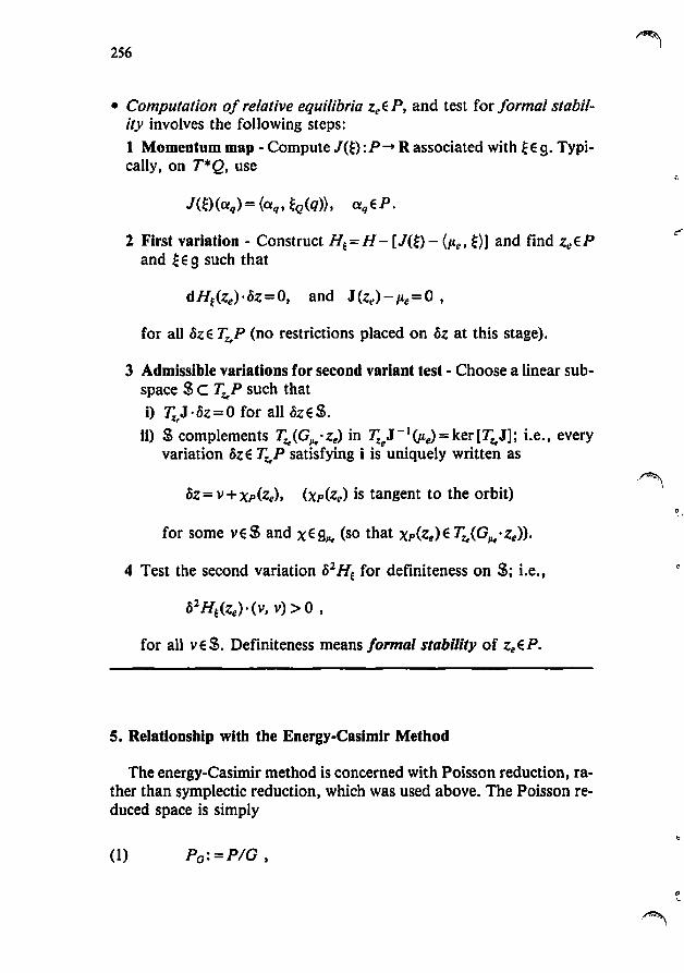
• Computation of relative equilibria zeEP, and test for formal stabil­ity involves the following steps: 1 Momentum map - Compute J(~): P -+ R associated with ~ E g. Typi­cally, on T*Q, use

2 First variation - Construct HE = H - [J(~) - (p.e, ~)) and find Ze E P and ~ e 9 such that

for all l)zE T~P (no restrictions placed on l)z at this stage).

3 Admissible variations for second variant test - Choose a linear sub­space $ C Tz.,P such that i) 7;,J ·l)z=O for all c5zE$.

ii) $ complements Tz.,(G~·ze) in 7;eJ-1(p.e)=ker[Tz.,J); i.e., every variation l)z E Tz.,P satisfying i is uniquely written as

c5z = v + Xp(ze), (Xp(ze) is tangent to the orbit)

4 Test the second variation 15 2 HE for definiteness on $; i.e.,

for all ve$. Definiteness means formal stability of zeEP.

5. Relationship with the Energy-Casimir Method

The energy-Casimir method is concerned with Poisson reduction, ra­ther than symplectic reduction, which was used above. The Poisson re­duced space is simply

(1) Po: = PIG ,

" '.

Q

257

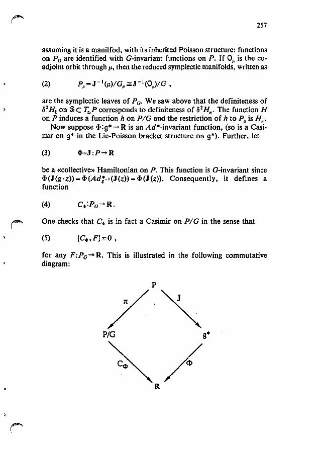
assuming it is a manilfod, with its inherited Poisson structure: functions on Po are identified with G-invariant functions on P. If 01' is the co­adjoint orbit through p., then the reduced symplectic manifolds, written as

are the symplectic leaves of Po. We saw above that the definiteness of 02 H~ on $ C T~P corresponds to definiteness of 02 HI" The function H on P induces a function h on PIa and the restriction of h to PI' is HI"

Now suppose cI>:9* -. R is an Ad*-invariant function, (so is a Casi­mir on 9* in the Lie-Poisson bracket structure on 9*). Further, let

(3) cI>oJ:P-'R

be a «collective» Hamiltonian on P. This function is G-invariant since cI> (J (g. z» = cI> (Ad;-, (J (z» = cI> (J (z». Consequently, it defines a function

(' One checks that C4> is in fact a Casimir on PIG in the sense that

(5) [C4>' FJ = 0 ,

for any F:Pa -+ R. This is illustrated in the following commutative diagram:

PIG s*

/ /~

R

258

Assume that zeEP is a relative equilibrium, so that there is an asso­ciated mUltiplier ~ E g, as above. Furthermore, assume that there is at least one function ~e:g* ~ R satysfying

(6)

Then, the functional

h+C4>.:PIG~R

has a critical point at [Ze] = 1I'(ze) where 1I':P~ PIG is the projection. The energy-Casimir method is essentially a test for definiteness of the second variation

on the tangent space 1it,IPIG to orbit [ze] EPIG; see Holm et al. [1985]. Normally one chooses a <Pe satisfying (6) to optimize the defi­niteness of (7).

For any ~e satisfying (6), the restriction of the second variation (7) to 1(Z.)P,.., the tangent space to the symplectic leaves in PIG is equal to the second variation of H,.. at [ze]. This is simply because H", = hi PJ" H,.. has a critical point at [ze], and C4>. is constant on P ",.

Thus, assuming (6) can be satisfied, the second variation (7) restricted to the reduced space, and the quadratic form induced by 02 H~ both coincide with 02 H",([ze]). Therefore, if the energy-Casimir method works, i.e., the form (7) is definite, then so is 02 H~(z) (restricted to $); i.e., the energy-momentum method works.

On the other hand, there are situations, such as those concerned with geometrically exact rod models, where the energy-momentum method can be applied successfully, but there appears to be no function ~ sati­sfying (6) and so the energy-Casimir method fails - see Simo, Posburgh, and Marsden [1988]. This also appears to be the essence of the results of Abarbanel & Holm (cf. Holm [1986]) and Morrison [1987].

Of course one can synthesize the energy-momentum and energy­Casimir methods; this is suitable when a group commuting with G is present. This results in the energy-momentum-Casimir method. it is im­plicitly used in Holm et al. [1985] for examples like the symmetric hea­vy top.

~-

v

259

As in the energy-Casimir method, for some problems in the infinite dimensional case, if one wants to deduce dynamical stability, convexity estimates for H~ on $ are required. The situation is analogous to that in Holm et al. [1985].

6. Example: The Rigid Body

We illustrate how to use the energy-momentum method by conside­ring the dynamics of a freely spinning rigid body. Of course we will re­cover the classic results that uniform rotation about longest and shortest principal axes are stable motions. The energy-momentum method is al­so used in more sophisticated examples of rotating structures, as in Si­mo, Posbergh and Marsden [1988].

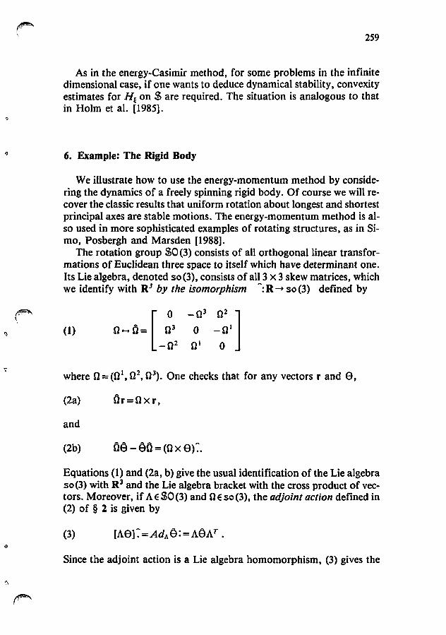
The rotation group $0 (3) consists of all orthogonal linear transfor­mations of Euclidean three space to itself which have determinant one. Its Lie algebra, denoted so (3), consists of all 3 X 3 skew matrices, which we identify with RJ by the isomorphism -: R ~ so (3) defined by

(1)

where 0 = (0 1,02,03). One checks that for any vectors rand S,

(2a) Or=Oxr,

and

(2b) OE) - eO = (0 x Sf.

Equations (1) and (2a, b) give the usual identification of the Lie algebra so(3) with R3 and the Lie algebra bracket with the cross product of vec­tors. Moreover, if A E $0 (3) and 0 E so (3), the adjoint action defined in (2) of § 2 is given by

Since the adjoint action is a Lie algebra homomorphism, (3) gives the

260

elementary identity

(4) A(rxs)=ArxAs,

for all r,sER J•

Given A E $0 (3), let v A denote an element of the tangent space to $0(3) at A. Since $0(3) is a submanifold of Gi!(3), the general linear group, we can identify VA with a 3 x 3 matrix, which we denote with the same letter. Linearizing the defining (submersive) condition AAT = 1 gives

which defines TA$0(3). We can identify TA$0(3) with so(3) by two isomorphisms:

i) Left translations - Given S E so (3) and Ae$O(3) we define (A, S) .... SA E TA $0(3) by setting

Thus SA is the left invariant extension of e. il) Right translations - Given 8 e so (3) and A e $0 (3) we define (A, 8) ....

o A E TA $0 (3) through right translations by setting

Thus 8 A is the right invariant extension of 8.

As in Simo, Marsden & Krishnaprasad [1988], the notation is dicta­ted by continuum mechanics considerations; uppercase letters are used for the body (or convective) variables and lower case for the spatial (or Eulerian) variables. Often, the base point is omitted and with an abuse of notation we write A~ and BA for ~A and BA, respectively.

The dual space to so (3) is identified with R l by using the standard dot product:

(7) 1

n·e=-tr[tiT~l . 2

() ,

261

This extends to the left-invariant pairing on TA $O(3) given by

(8)

We shall, thereby, write elements of so(3)· as fi, where nER3, (or 1r with ?l'ER3) and elements of T!$O(3) as

(9) fiA = (A, Ali) ,

for the body representation, and for the spatial representation

Again, explicit indication of the base point will often be omitted and we shall simply write Afi and 1rA for fiA and 1rA, respectively. If (9) and (10) represent the same covectoT, then

(11)

which coincides with the co-adjoint action. Equivalently. using the iso­morphism (2) we have

(12) ?I' = All .

The mechanical set-up for rigid body dynamics is as follows: the con­figuration manifold Q and the phase space Pare

(13) Q=SO(3); P= T·SO(3) with the canonical symplectic structure

i) The Hamiltonian H is the kinetic energy of a free rigid body. One shows in standard fashion (see for instance Marsden, Ratiu & Wein­stein [1984]) that

(14)

where n is the time dependent inertia tensor (in spatial coordinates)

262

and .H is the constant inertia dyadic given by

(15) .H= 1~ Qre/(.X)[IIXII 21-X®X]dJX.

Here, ~ C R3 is the reference configuration of the rigid body and (1ref:~ R the reference density. We regard H in (14) as a function H:SO(3) x so*(3)- R where so(3) == R3*. This is essentially equi­valent to regarding H as a function on P because of the isomorphism

(16) (A, 1I")ESO(3)=R3* .... (A, 1M) == 7rAE 71S0(3).

However, the former view, Le., H(A, 11"), is computationally more convenient.

ii) Invariance Properties - Making use of (12), H in (14) can be written in the convective representation (body coordinates) as

(17) 1 J H=-n·jJ- n 2

which reflects the (manifest) left in variance of H under the action of $0 (3). Thus left reduction by SO (3) to body coordinates induces a function on the quotient space 1"*$0(3)/$0(3) == so*(3). The sym­plectic leaves are spheres, Inl = constant. The induced function h on these spheres is given by (17) regarded as a function of n. The dynamics on this sphere is given by the usual picture obtained by intersection of the sphere IIII2 = constant and the ellipsoid H = constant.

iii) Momentum map - Consistent with the preceding discussion, we choo­se G= SO (3) acting from the left on Q= $0(3) by left translation, i.e.,

(18) i'(Q. A)=LQA= QA ,

for all A E $0 (3) and Q E G == $0 (3). Hence, the action of G = $0 (3) on p= 1"'$0(3) is by cotangent lifl of left Iranslalions. Since the infinitesimal generator associated with ~ E so (3) is obtained as

(19) ~so(3)(A) = - exp [t~] A = ~ A , - d _ I -dt 1=0

()

263

by Proposition 2.1 the momentum map associated with the left SO (3) action is given by

Thus, (20) gives

(21) J(i.J=i, or Ja)=7I"'~'

This constitutes our fIrst step in the application of the energy-momentum method in the box. According to the second step of the energy-momentum method, we consider

(22)

and examine its critical points. To compute the first variation we recall that although i A E 1'* SO (3), including its base point A, are the basic va­riables, it is more convenient to regard H~ as a function of (A, 71") E SO (3) X R3* through the isomorphism (2).

Thus, let i~ == (Ae, ieAe)E 1'*SO(3) be a relative equilibrium point. For any MER3 we construct the curve

which starts at Ae since

(24)

Let 071" E R 3,.. and consider the curve in R 3* defined as

264

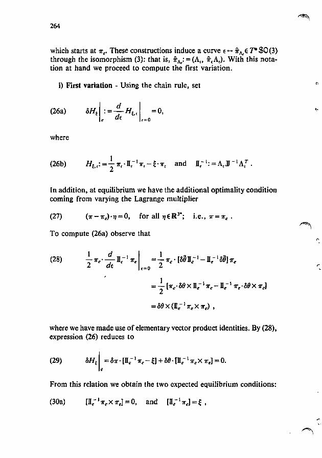
which starts at 1Te' These constructions induce a curve p-. 1r~E T"$0(3) through the isomorphism (3): that is, 1r~: = (Af' 1r(Ae). With this nota­tion at hand we proceed to compute the first variation.

i) First variation - Using the chain rule, set

(26a) OHf-1 : = !!..... HE .• I =0, e de .=0

where

(26b) and n-I'=A .u-IAT t· f E •

In addition, at equilibrium we have the additional optimality condition coming from varying the Lagrange multiplier

To compute (26a) observe that

(28)

where we have made use of elementary vector product identities. By (28), expression (26) reduces to

From this relation we obtain the two expected equilibrium conditions:

(')

265

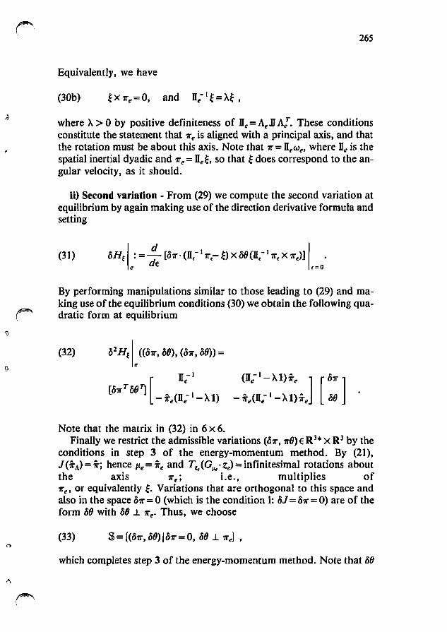
Equivalently, we have

where X> 0 by positive definiteness of He = At'.D A[. These conditions constitute the statement that 1C't'is aligned with a principal axis, and that the rotation must be about this axis. Note that 1C' = Hewt" where He is the spatial inertial dyadic and 1C'e=Ht'~, so that ~ does correspond to the an­gular velocity, as it should.

ii) Second variation - From (29) we compute the second variation at equilibrium by again making use of the direction derivative formula and setting

(31)

By performing manipulations similar to those leading to (29) and ma­king use of the equilibrium conditions (30) we obtain the following qua­dratic form at equilibrium

(32)

Note that the matrix in (32) in 6 x 6. Finally we restrict the admissible variations (01C', 7r8) E R 3* X R3 by the

conditions in step 3 of the energy-momentum method. By (21), J (fr A) = fr; hence Ile = fr e and T z. (G ,,; ze) = infinitesimal rotations about the axis 1C'e; Le., multiplies of 1C'e' or equivalently ~. Variations that are orthogonal to this space and also in the space 01C' = 0 (which is the condition i: oj = 01C' = 0) are of the form 00 with 08 .L 1C'e. Thus, we choose

which completes step 3 of the energy-momentum method. Note that 08

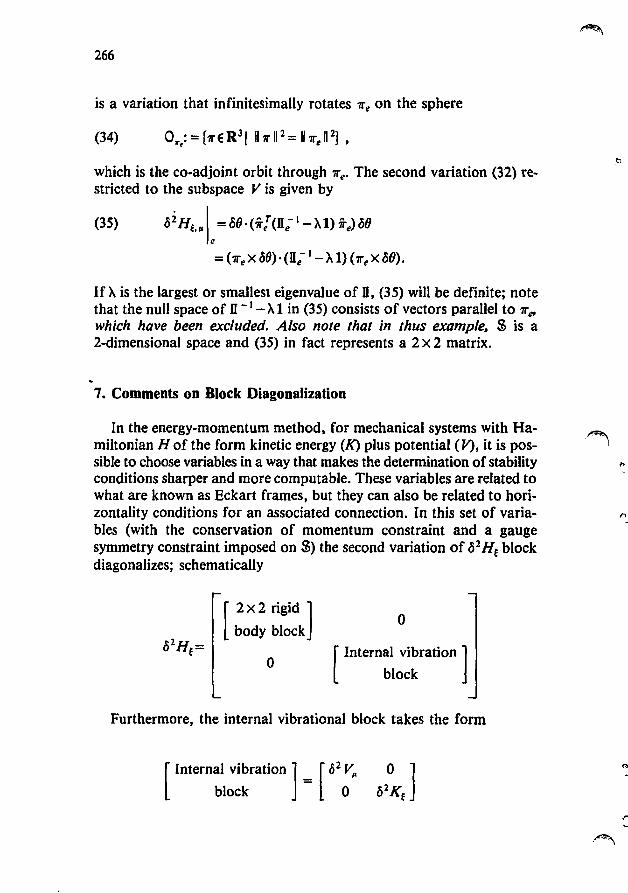
266

is a variation that infinitesimally rotates 7re on the sphere

which is the co.adjoint orbit through 7re• The second variation (32) re­stricted to the subspace V is given by

(35) oiH~,,{ =oO·(i!(lle- I ->.l)ie)08

= (1re X 08)·(De-I ->.l) (7re X 08).

If >. is the largest or smallest eigenvalue of D, (35) will be definite; note that the null space of n -I - >. 1 in (35) consists of vectors parallel to 7reo

which have been excluded. Also note that in thus example. $ is a 2-dimensional space and (35) in fact represents a 2 x 2 matrix.

7. Comments on Block Diagonalization

In the energy-momentum method, for mechanical systems with Ha­miltonian H of the form kinetic energy (K) plus potential (V), it is pos­sible to choose variables in a way that makes the determination of stability conditions sharper and more computable. These variables are related to what are known as Eckart frames, but they can also be related to hori­zontality conditions for an associated connection. In this set of varia­bles (with the conservation of momentum constraint and a gauge symmetry constraint imposed on $) the second variation of 02 H~ block diagonalizes; schematically

[ 2 x2 rigid] body block

o

o

[Internal vibratiOn]

block

Furthermore, the internal vibrational block takes the form

[Internal vibratiOn] = [0 2 VI' 0]

block 0 02Kt

n

267

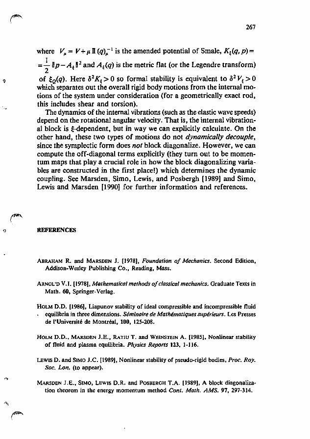
where V,. = V + p. n (q}I'-1 is the amended potential of Smale, K~(q, p) =

=..!.. Up-AeU2 and Ae(q) is the metric flat (or the Legendre transform) 2

of ~Q(q). Here ~2 Ke > 0 so formal stability is equivalent to ~2 Ve > 0 which separates out the overall rigid body motions from the internal mo­tions of the system under consideration (for a geometrically exact rod, this includes shear and torsion).

The dynamics of the internal vibrations (such as the elastic wave speeds) depend on the rotational angular velocity. That is, the internal vibration­al block is ~-dependent, but in way we can explicitly calculate. On the other hand, these two types of motions do not dynamically decouple, since the symplectic form does not block diagonalize. However, we can compute the off-diagonal terms explicitly (they turn out to be momen­tum maps that playa crucial role in how the block diagonalizing varia­bles are constructed in the first place!) which determines the dynamic coupling. See Marsden, Simo, Lewis, and Posbergh [1989] and Simo, Lewis and Marsden [1990] for further information and references.

~ REFERENCES

. '\.

ABRAHAM R. and MARSDEN J. [1978], Foundation 0/ Mechanics. Second Edition, Addison-Wesley Publishing Co., Reading, Mass.

ARNOL'D V.I. [1978], Mathematical methods o/classical mechanics. Graduate Texts in Math. 60, Springer-Verlag.

HOLM D.O. [1986], Liapunov stability of ideal compressible and incompressible fluid . equilibria in three dimensions. Seminaire de Mathematiques superieurs. Les Presses

de l'Universite de Montreal, 100, 125-208.

HOLM D.O., MARsDEN J.E., RATIU T. and WEINSTEIN A. (1985), Nonlinear stability of fluid and plasma equilibria. Physics Reports 123, 1-116.

LEWIS D. and SIMO J.C. [1989], Nonlinear stability of pseudo-rigid bodies, Proc. Roy. Soc. Lon. (to appear).

MARSDEN J .E., SIMO, LEWIS D.R. and POSBERGH T.A. (1989), A block diagonaliza­tion theorem in the energy momentum method Cont. Math. AMS. 97,297-314 .

268

MARSDEN J.E .• RATIU T. and WEINSTEIN A. [1984]. Semi-direct products and reduc­tion in mechanics. Trans. Am. Math. Soc. 281. 147-177.

MARSDEN J.E. and WEINSTEIN A. [1983]. Coadjoint orbits. vortices and Clebsch va­riables for incompressible fluids. Physico 7D. 305-323.

MORRISON P.J. [19871. Variational principle and stability of nonmonotone Vlasov­Poisson equilibria. Z. Naturforsch. 428 1115-1123.

MORRISON P.J. and ELIEZER S. (1986). Spontaneous symmetry breaking and neutral stability on the noncanonical Hamiltonian formalism Phys. Rev. A 33. 4205.

SIMO J.C .• LEWIS D.R .• MARSDEN J.E. (1990). Stability of Relative Equilibria I: The Reduced Energy-Momentum Method (Arch. Rat. Mech. An .• to appear).

SJMO J.C .• MARSDEN J.E. and KRISHNAPRASAD [1988]. The Hamiltonian structure of nonlinear elasticity: The material. spatial. and convective representations of solids. rods, and plates. Arch. Rat. Mech. An. 104, 125-183.

SIMO J.C., POSBERGH T.A. and MARSDEN J.E. (1988), Nonlinear stability of geome­trically exact rods by the energy-momentum method SUDAM Report # 88.1. Divi­sion of Applied Mechanics. Stanford University (to appear in Physics Reports).

WAN Y.-H. and PULVIRENTE M. [1984]. Nonlinear stability of circular vortex patches. Commun. Math. Phys. 99, 435-450.

WEINSTEIN A. [1984]. Stability of Poisson-Hamilton equilibria. ConI. Malh. AMS 28, 3-14.

J.E. MARSDEN - Department of Mathematics. University of California. Berkeley. CA 94720. Research partially supported by DOE contract DE-AT03-88ER-12097 and MSI at Cor­nell University.

J.C. SIMO - Division of Applied Mechanics. Stanford University, Stanford. CA 94305. Research partially supported by AFOSR contract 2-DJA-544 and 2-DJA-771.