LA-lJR3ti=34’35 (btlf y 0/:’w (4- -/

LJ9 Alamcs P4al!onal LaDoralOFti 3 oDeraled byIhaUnwWllfy of Cnhfornla fOr Ihc UnMd SIaIos Oopmfmonl of Energy under Confracl w.7405. ENG Ie

LA-UR--9O-3495

DE91 001967

TITLE MONTECARLOMETHODSANDAPPLICATIONS IN ~uEAR PHYSICS

AuTHOR(S) J. Carlson, T-5

SUBMITTED T@ PROCEEDINGSOF THE INTERNATIONALSUMMERSCHOOLON THESTRUCTUREOF HADRONSANDHADRONICMATTER,DRONTENTHE NETHERLANDS,AUGUST4-17, 1990, GIVEN AS ANINVITED SET OF TALKS

lNSX’l,AiMKR

“1’hiircp,rl W:IS ptt-pilrcd iI\ JIImXXIIIIIIIII w,)rk \pmsIIIc(l hy JII :IgCIICY id thr lIIIIICtl Stnfcs

( hwcrrlnwnl NrIIII(. I fhr 1111111,11\l.Ilr\ (;,, VCI,IIIWIII ,1,,1 ,,11, ;I~C,,{-V l}ll. rc,,f, ,1,,, ,,,,} ,,1 Ihclfrlllldtlbrc\, ul,lht-\ ,Inv w:trf,lnf). rqprc\\ ,11 1111111, ,1, IM .IS\IIIIIC. ,IIIJ IcE.11 II, 111111,v III fr~pmwhllll\ full thl’ ,1(,111,,, ,, \,)utlf)lrlrntx\, *II II\rlultlc ,11 .IIlb Inl,tlrl).lf,(tlj. ,Ipp;II.II IIf, lIIIMIII, l. III

Ill,. ,... ,11.. l,wil, ,)r :Cpl(.,,rfll,. IIIJI II. 11., *11111(1 ,1,,1 IHIIIII~IO pIIIIICl\ 41WIICII ,I@I1.. I(rf,-,

1.1114, 11( ’lrlll l,> .411$\l). vIflt 8tlllllllrlt 1;1 I p,tmluul, Illtn (.,,, ,,1 ,,., V,, (’ I)\ 11,,,11’,,,,,,,,,, l,,,,lr,,,,,, ~,!ll,llllll ,1, Illlv, , 811IIlllrlvlw ,Iow.! 11,,1Iltn!’,,,,l ,1) t ,),,.,1)1,,1(. ,,, 1,,,,,1, ,1, ,.,,,l,l, .r,,, ~,,l, ,,,, ,,,,,111(.ll,l,lll!lll,!)1I,l!!ll, ,lp ll\ It,,, I ‘!l,l (-,1 %1,,1,., I ;I,, r,,,,,,,.,,1 ,,, ,, !:, ,,p,,.,,, , n,,. ,(.,,l Ihr \trw.

.!1)41 ,Il,llltam, ,,1 tlllll I,l, t,vl,l,,,wll hrlvbll IhI 11111lIctv\\,Ir Il\ .I,IIv ,If Irllrt I III,IW ,11 thrII, IIIIvI \t,Ilr\ (,atb Is II1lIlrf)l ubt .Ill\ l~rlltt Ihrlt,,lf

,., , !~,... . ,. .;

‘,’1 “t’”l., i,’

~J\\v 1,) ‘) IW

lk)~~lla~~s Lo.Alamo.,NewMexi..87545 ,)LOSAlamos National Laboratory ,

MONTE CARLO METHODS and APPLICATIONS lN NUCLEARPHYSICS

J. CarlmnT5 }(ail Stop B2$3

Los .Alartios Sational LabLos Alarnos, X)1 37W5

Abstract

Monte Carlo methods for studying few- and many-body quantum systemsare introduced, with special emphasis qivmr to their applications in nuclearphysics. Variational and Greens function Monte Carlo methods are presentedin some detail. The status of calculations of light nuclei is reviewed. includingdiscussions of the three- nucleon. interaction, charge and magnetic form factors,the coulomb sum rule. and studies of low-energy radiative transitions,

1. Introduction

In these lectures 1 will introduce \lonte (;arlo methods as applied to few- anlimany-body’ quantum systems, and in particular to few-body problems in nllclt*itrphysics, While 1 will not be ahlr= to go into some of the technical details, 1 hopeto provide you v’ith a basic understandiliq uf the principles involvmi. [ also hop~to cunvince you that there are many intriguing questions that ran he addrmw!I)y studying light nuclei, and that Jlonte (’arlo methods provide a u~eflll way ofattm.king these few-body problems.

I will discuss Variational’+ (Y MC) and (;rem’s function Monte (’arlo5””7(G F\lC).\“\l(,’ and (i F\l C are fairly general; they are often used in condensed matter&” mnd,~tomic phywcs “.’:’ in addition to their applications in nilclear physics. ~hcse mrth.I)(Is ilre AISOclweiy related to the finitet.emprraturr nwthods used in both cc)n(lensml

II]attor and lattice QCD, Nuclear physics apl)licatious include hvprrnucki AII(Ivar.IOIIS {“(JllStltUent ql!?rk TIO(k19 Ill a(hlltloll 10 ll~ht llu~h?i. :\tte[npts arc also I)vl[lg

II IaIIO to apply generalizations of these mf’thods to heaviw nur-lci, h~lt 1 will rmtrl(”t.lll~W’[fh) feW-hOdY prohkm~ in thCW h! IIWS.

I will iil~() cowr the structure of thr grolln(l st,atm d light nllclri, inrl~l(linq IwI)-I)()(ly (.orr(’l;itions,” IIlt’ importance of thr 11’nsor forrt’ , MI(I th(~ rlfect of tllrc’t’.fllll”l(k)ll

il]l,t’ractiotls, I will l)rwwnt ralcllla~imls tJf’I111’( ‘I)lllt)Illl)311111,011P of ttlr I)f’st f’xpwl

llwntill” ‘d irltlications 0( stmrlg (wrrr’lilli~)lls willlifl t.hl’ Ilucltw, In wlditi(m. 1 willl~)lii.1]Ilpon mmkls of thr cllrrrvlts, ill(.llll!ill~ l,wo lIIIIiVl“~largeA[l(lcurrrnt. ol)f’rillllr~,

I

and their importance in describing electromagnetic forr,i factors. FinallY, I will lookat Monte CUIO methods for calculating low-energy scattering; and in particular atrecent calculations of neutron radiative capture on 3He.

Fiwl. however, 1 will present the bajic Monte Carlo algorithms. Tt.e most im-portaat principl- will be described along with the simplest practical algorithms.

These tools should z+.I1owyou to explole at least simple systems on your own. Oneshould always keep in mind, though, that for more complicated problems. better\lonte Carlo methods (improved sampling techniques, etc. ) can be vital, making thedifference between a robust solution with good statistical accuracy and a result withstatistical errors so large as to render the calculation virtually meaningless. I hopethat the references will be sufficient in number and detail to allow anyone interestedto easily go beyond the rel.atlvely crude algorithms given here.

‘~ Nuclear Hamiltonian-.

Before studying the Monte Carlo algorithms, 1 would like to spend a little timediscussing the nuclear Hamiltonian and the difficultiu involved in determining itseigenstates We ~ill employ the traditional description of the nucleus as a system0[ non-relativistic nucleons interacting through strong spin- and isospin-dependentnllclear ir;teractions, The solutions of the !%hroedinger equation

(1)

t.i~[l Ihen be used, along with an appropriate currmit operator. to determine many~]ruperties of the nucleus. The potential is determined by fitting two- (and possi-bly three- j body experimental data. It includ~ the onepion-exchange term at longIIist antes, and in some cases is modeled as a set of one- boson exchanges at shortm1’t lsta:lo=s. Clearly this model leaves out some interesting physics: internal degres of

frrwlom (such as the delta r~onance) have been suppressed and the efkts of meson~~~[’]l;~ngehave been absorbed into the potential. Each of these simplifications pro-I!IIIW important cthcts even in ground-state properties, as we shall we. Nevmthel_s,~.u,II [Ilis sl[llple Iloll-relativistic treatment contains a great deal of physics.

I“hr I.w-lwdy interaction can he writt~n as a gum of spin-isoxpin d.qmldentt)l]~’r;il~)r(.)$, multiplied hy functions of th~’ pair ~~paratlon ‘IJ:

( ):, =:(1,,7,lflJ,s,J,l. S,,,[,1S!,,l.~,,l./J~7,fl,}@{ltrir,} (:!)

spins of the nuckms, and ri and r, are similar matric- for the isospins. The tensoroperator S,J is 3~i t ~ijej ;ij-&im u, and L . SiJ is the spin-orbit interaction, whereL represents the relative angular momentum of the pair, and S the total spin. Theoperators L . S~j and L~, determine the spin-orbit squared and angular momentumsquared dependence of the interaction, respectively.

All modern interactions ( Argonne, 17 ~nn,’a Nijmegenlg ...) may be written ina similar manner. Terms up to first order in the momentum (L oSiJ ) are uniquelyindicated by the data, but the choice of the more non-local operators varies in dif-ferent interaction models. We will concentrate primarily upcn the Argonne VI-1

interaction which employs the particular choice given above. It has been constructedto minimize the importance of the non-local terns in the in ;eraction, and includesa one-pion interaction at long distances, an intermediate range attraction with therange of a two-pion-exchange, and a short-range phenomenological repulsion.

Some terms in the Argonne V14 interaction are shown in figure 1, for simplicityI only present the central (momentum-independent) and tensor terms in the inter-action. Two primtuy features that are common to all NN interaction models shouldhe Jtremxi. The most striking feature is the strong repulsive core at short distances.This presents some difficulties to mean-field or pert urbative calculations, but it ispossible to treat the strong correlations induced by th- interactions with MonteCarlo. In fact, I will show results from condensed matter physics for systems of fiftyto several hundred very strongly-interacting particles. The repulsive core in thesesystems is e~en stronger, in relative terms, than that in the NN interaction.

6s0

Ma

no

154

50

-pt5-l0.0 0.s

. . ..—. —-... -— Ito ! .s

* (fro]

V 14 intorartion.

50

-M

-MO

-4s0

“\\,.,,.,,

‘...,~-... .. ... ..._ .. . .. . .. .... . w

Figure lb) Tensor terms in the Argonne V14 interaction.

The secc nd feature, also crucial to nuclear physics, is the strong spin- and isospin-dependence of the interaction. The potential can be quite different for differentcombinations of total spin and iaoapin (note that the S,T = 0,0 and 1,1 central termsoccur in negative parity statea, and consequently always appear in combination withL!, terms), Results are also very sensitive to the tensor force, in fact we find thatthe tensor force provides ~bout 2/3 of the total potential energy in light nuclei,(’consequently, any wave function which ignores the strong tensor correlations will notreproduce any of tnc bound states. The strong state-dependence of the interactionis also what limits our calculations to light nuclei, at least for the present, Tounderstand why, we will need to look at ttlc structure of the wave function.

Before proceeding to the wave function, though, I should mention the three-I]ucleon interaction (TNI), The T,NI will be discussed in more detail in a later section,ilt this point I would simply point out that the pr~ence of a thr= nucleon interaction

is mmntially required by the fact that we are suppressing the internal structure ofthe nucleons. The importance of the three-nuchmn interaction (TNI) can be tmkmM a Incasure of the importance of ignoring the internal d~grea of frmdom in thenllcleml, the quarks, At long distances the form of the TN1 is assumed to aris~ frompion I’xchanges and excitations to virtual deltas, its prm. ise strmgth is tit to I.IN*t hrcr- body binding energy. 2 We will find that the ‘rl~l is much less impi)rtant tha[l[he twO-l]llcl~n inter~tion, typically (k’,Jb)/(t{J) S fi’%0. Ihw?v?r, it do= Provkk a

~ig[lifican~ fraction of the binding enmgy in light I)llclei, M the binding em=rgy renultsfrom a srnxltive cancellation of Iargr kinetic MI(1potential energy tmrns.

3. Variational Wave Function9

Given the Hafiltonian of Eqs. 1-3, any wave function can be decomposd intoa sum over spin-isospin states times functions of the coordinates of a,ll particles:

The sum over states 1 runs from 1 to 2AA!/N!Z! for a system of N neutrons and Zprotons (A= N+ Z). The factor 2A comes from the spins (each of A spins up or down)and a factor of ,4!/N!Z! from the isospin. The isospin factor is smailer because ofcharge conservation, the total number of protons or neutrons remains constant. Notethat we are not exploiting good overall isospin, which could reduce the number ofcomponents further at the cost of a more complicated basis, Calculations employa basis of definite third components of spin and isoapin for each particle. This isdiscussed in more detail in the Appendix.

Solving the Schroedinger equation now entails solving many coupled differentialequations for the complex amplitudes @l(R). For A=3, Faddeev methodsa-az canbe used to solve for these amplitudes explicitly, although they of course employ adifferent basis of states. As the number of nucleons increaaea, however, It becomes leasand less fe~ible to solve dir4y for the amplitudes #l. (he possibility for going tolarger systen~ is to develop approximate variational solutions for the wave function,this is the alternative we will discuss first. Note that the threebody nuclei providea very important test for any variational calculation since they can be calculated‘exactly’ with Faddeev methods.

Any variational calculations proceeds by first making an ansatz for the form Jfthe wave function and then minimizing the expectation value of the Hamiltonian

(5)

wi~h respect to changes in the variational parameters {a} embtdded in the form - fvariational ( trial) wave function VT {a}. The important phyoica required in this caseimludcs ( I ) an accurate form for the wave function as two nucleons ue brought closetogether. (2 ) a reasonable treatment of the spin- isospin correlations induced by theilltfiraction, ad (3) the correct asymptotic wave function M one nuchmn is pulhxlilwav from the remaining nucleons.

:\ generalized JMtrow form for the wave function carIall ii this physics:

()l*r) =1$ ~F,, 10).

1<1

be used which incorporate

((i)

III this rquation, O is an anti-symmetrizml Slater determinant, the F’,, are ~,tatetl~pm(lmt) two-hod y rorr~lalion op~ratcws, and S is a symrnetrization operato~. ‘rh~

5

symmetrization operator indicat- a sum Gver all orders of terms in the product, andis required since the correlation operators between different pairs do not commute.

For light nuclei, it suffices to choose 0 as a spin-isospin vector independent of al]

spatial coordinates:

0(2H) = A[(n T)l(p T)z], (7)

0(3H) = A[(n L)l(n T)2(p T)3], (s)4( 4He) = A[(n L)i(n T)2\p l)3(p T),]. (9)

In this notalion, A is an anti-syrnmetrization operator indicating a sum over ailpossible interchang~ of particles with appropriate signs. For larger nuclei ( A >4 ),spatial degrees of fr~om must be incorporated into the 0. Here, however, we canchoose the pair correlation operators F’,j to give the correct asymptotic conditionson the wave function.

We choose the pair correlations to have the following form:

F,, =[( )]

~(rt,) ~ + ~ w(r,,,R)uk(r,,)O~ ,k

(10)

where the sum over operators k runs over all momentum-independent operators inthe interaction ( Eq. 3). The pair correlations f’ and Uk are obtained by solvingtwo-body differential equations of the general form:3r4

(11)

where ,\(r) contains several variational parameters. In the qpin singlet cnannels, twouncoupled equations are solved, one for T=(l and one for T= 1. [n the spin tripletchannels, coupled equations are solved for the central and tensor correlations. Once

the equations arc solved in the various channels, linear crtnbinations are obtainedwhich can be cast in the operator form of Eq, 10,

The function A(r) is a woods-saxon at short distances. The width and range ofthe woods-saxon are variational parameters, At long distances its form is determinedhy reqlli ri,lg that the wave function have the correct asymptotic properties as one

IIIICleOII is removed from the ret. The separation energy which determines thettxpt~ncrltial decay is an additional variational parallieter, as is the ratio of the lensor;ln~l (’rtltral correlations at long distance,

[’he Ul correl~tion in Eq, 10 is a three-body term Ivhich reduces the strength oft INSl)pprator-dependent two-hod, correlations for some ccmfigurations of ,: ~ nucl~.l)l]\, 1 It lh’l)~lld~ [lot only on the pair distance r,, but aho on the positions of a!i thr1)1 hrr l);~rtit.ltw. iimpiriral]y, it h~ prowl useflll to parametrize U1as

ti ,(r,,, R) = r-1[ l- t-(1

L)’) Pxp( -t,,l?,,k) ,k#l,) I{,)k

t;

withi?,lk = ‘lJ + PA + rjk. (13)

The values of tl, t2, and t3 are determined variationally. [n principle they could beadjusted independent ly for each pair correlation operator (each k). but in practicethey are usually chosen to be the same in all channels.

The exact aeuteron wave function can be cast in the form of Eq. 6. In thi~ case thethree-body correlation U3 is replaced by the identity, and the function A(r) is simplya constant, the deuteron binding energy. The functions y(r) is u(r), the s-wave partof the deuteron wave function. The tensor term fi(r)us(r) i~, withir, a normalization

constant, w(r), the d-state component of the wave function. The deuteron’s wavefunction is worked out in the 3rd component of spin and isoapin basis in the Appendix.For the deuteron, of course, the amponents of the wave function are only functionsof one variable, so that calculating expectation valuea of any operator is relativelye-y. For larger systems, though, this becomes progreaaively more difficult. Hence,we rely upon ~Metropolis Monte Carlo to calculate the necessary integrals

4. Variational Monte Carlo

Given a parametrized wave function in the form of Eq. 6, (H) must be minimizedas a function of the variational parameters. Evaluating (H) involv~ computingmany 3A dimensional integrals, so we turn to Monte Carlo methods, in particular toMetropolis Monte Carlo. Monte Carlo methods in general become more valuable ssthe dimension of the space ~ncre~es, and their efficiency depends to a great extenton the quantity to be measured and also upon the care with which they are applied.

}fonte “Carlo methods as appliei here are described in some detail in a book byWhitlock and Kales.23 I can only provide some of the kmcs here. Those interestedcan consult this book and other standard references to determine optimum methodsfor sampling various distribution functions, and also for more detailed discussionsof the Metropolis and Green’s Function Monte Carlo methods. Also, R. B. Wiringaand 14 have written a bock chapter which contains quiteVariational Monte Carlo methods as applied to light nuclei

program.

\,, L“.MC’- Gencml Method

specific discussions of theand also includ= a sample

\letroPoh Monte Carlo24 is designed to evaluate ratios of integrals such as:

(0) = J W’(R)(7( R)cfR

[ W’(R)cfR ‘(14)

wi~er~ IV( R) is a positive definite function, \Vhile such a form may seem rather lim-itmi, ill fart many inter=ting physics probl~ms can be written in this way, Classicalstatistical mechanics is a primary example. If We take W(R) to be VXP(-3~) and U

7

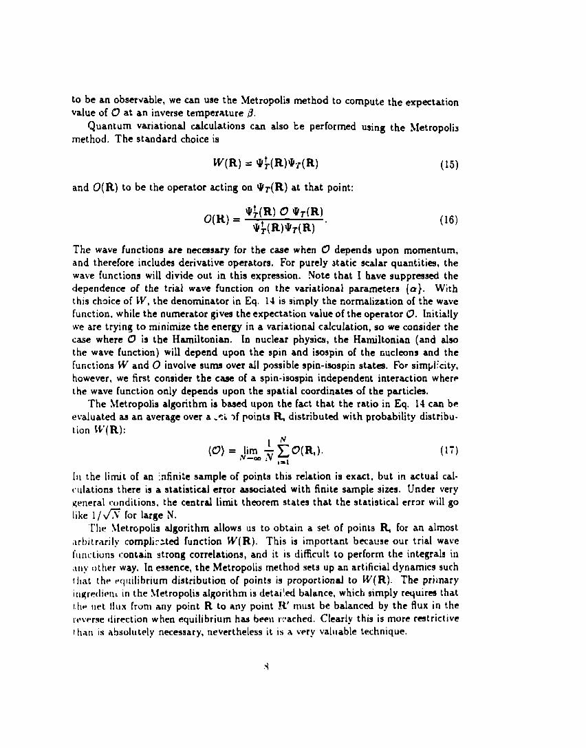
to be an observable, we can use the Metropolis method to compute the expectationvalue of 0 at an inverse temperature i?.

Quantum variational calculations can also be performed using the Metropolis

method. The standard choice is

W(R) = U+(R) WIT(R) (15)

and O(R) to be the operator acting on *T(R) at that point:

O(R) = II+(R) O WT(R)

NI~(R)*T(R) “(16)

The wave functions are necessary for the case when 0 depends upon momentum,and therefore includes derivative operators. For purely Jtatic scalar quantities, thewave functions will divide out in this expression. Note that I have suppressed thedependence of the trial wave function on the variational parameters {Q}. Withthis chaice of W, the denominator in Eq. 14 is simply the normalization of the wavefunction, while the numerator gives the expectation value of the operator 0. Initiallywe are trying to minimize the energy in a variational calculation, so we consider thecase where 0 is the Hamiltonian. In nuclear physics, the Hamiltonian (and alsothe wave function) will depend upon the spin and isospin of the riuchmns and thefunctions W and O involve sums over all possible spin-isospin states. For simplicity,however, we first consider the case of a spin-isospin independent interaction wherethe wave function only depends upon the spatial coordinat- of the particles.

The Metropolis algorithm is based upon the fact that the ratio in Eq. 14 can beevaluated as an average over a .5L >f points ~ distributed with probability distribu-tion W’(R):

(17)

ill the limit of an Infinite sample of points this relation is exact, but in actual cal-[.lllations there is a statistical error associated with finite sampie sizes. Under very

Keneral renditions, the central limit theorem states that the statistical error will golike l/JT for large N.

The \letrGpolis algorithm allows us to obtain a set of points ~ for an almost,lr})itri~rily complicz ted function W(R), This is important because our trial wave[Ilnctions i:ontak strong correlations, and it is difficult to perform the integrals inii[)~ other way. In essence, the Metropolis method sets up an artificial dynamics mchthat the twlltilibrium distribution of points is proportional to W(R). The primaryillurf?(ll(’ill in the \letropolis algorithm is detailed balance, which simply rquir~ that.t l~IJ[let tlux from any point R to any pointrrvrrse direction when equilibrium has beent han is absolutely necessary, nevertheless it

i

R’ mu9tr:’ached,is a very

be balanced by the flux in theClearly this is more restrictivevall]able technique,

A random walk algorithm can then be developed which satisfim detailed balanceand gives an equilibrium distribution proportional to an arbitrary W(R). Suppose wcstart at RI, and construct a random walk in which each step contains two elements,

a proposed (trial) move and an acceptance/rejcxt ion step. First, a point R~ is chosenfor the trial move wit h a transition probability T( RI ~ R,), and second, this trial

move is accepted with probability A(RI + Rc ). If the move is accepted R2 is setto Rt, otherwise R2 is set to R1. The whole process is then repeatd (the next stepbeginning from R2) until the walk has reached equilibrium and a sufficient numberof points have been generated to obtain accurate results.

A little thought will convince you that detailed balance imposes the followingcondition on the random walk if it is to generate an equilibrium distriblltion propor.tional to W(R).

W(R1)T(R1 ~ Rz)A(R1 - R2) = lV(R2)T(R2 ~ RI)A(R2 ~ R,). (18)

The left hand side of this equation is the flux from Rl to R2, it is given by the productof the probability of being at RI (which we require to be IV(R1 )), the probability Tof proposing a move from RI to R2, and the probability A of accepting that proposedmove. The right hand side of the equation is the total flux in the opposite direction.

A very simple choice for T(R1 + R~) is a constant ( l/L3) within a 3A dimen-sional cl..’Dewith side L. This transition probability is trivial to implement. For eachcomponent i of the 3A dimensional vector, simply take:

R,, = Rl, + 2L(c, - 0.5), (19)

where the (, are random numbers evenly distributed between O and 1. V~ith thischoice of T, it is obvious that T(R1 e R2) is identical to T(R2 ~ RI). If R2 iswithin the box centered at Rl, Rx is also within the box centered upon RI andboth transition probabilities are equal, but if R2 is outside the box both transitionprobabilities are zero.

\k’ith this choice for T detailed balance become particularly simple. We cansatisfy Eq. 1S by taking

[1W’(R2)A(R, ~ R2) = min 1,— .

\\ ’(R,)

Xote that the acceptance probability must always be betweenfunction W is greater at the new point than at the old, the

(20)

zero and one. If themove will always be

accepted. Othe;wise, it will be accepted with a probability equal to the ratio of thefunctioils, Note that a total of 3A + 1 random numbers are needed at each step int,}w walk, :J.4 to choose a trial step and one to accept or reject it.

The r-ultinq algorithm. ~mploying a qt=neral transition probability T, can bewritten dd,vn very simply:

1.

~.

3.

4.

Givena 3A dimensional coordinate ~,generate atrial coordinate point R,with probability l’(~ 4 R().

Calculate the quantities WOW Z’(RI + R~), and T(R, +Rl), thetransition probability for the reverse step. The acceptance probability is givenby the expression:

WU)T(IL + W)A(R1 ~ Rl) = min{l,

CV(R1)T(Rl 4 Rt) } (21)

Accept or reject the move with probability ~. lf the move is accepted, set ~+1equal to Ri, otherwise set it to W.

Calculate all quantities of interest (the Harniltonian, etc. ) at ~+,, adding thecontributions to the average over all points (Eq, 17).

The random walk will only generate points distributed with probability W’(R)after it has reached equilibrium. Convergence to equilibrium is an important con-sideration that must be tested in each calculation. All results obtained prior to

equilibrium should be disregarded in the averages above. This is usually not a prob-lem in light nuclei aa several hundred steps normally suffice unless one starts from apathdogicai initial point (one nucleon 20 fm from the othera, foi example). A goodway to test for equilibrium is to compute the average over ‘blocks! of consecutivepoints in the random walk consisting of several hundred points to several thousandpoints each.

Eventually, the averages within each block should settle down to a constant plusa (hopefully small) fluctuating term. If the blocks are large enough, the averageashould have a normal distribution centered on the true mean, and the error can beestirr.ated from th,=m using the central limit thmrem:

where A(cJ) is an ~timate of the error in determining (0) and M is the total numberof blocks, The exprasicm involves the average of the square of the estimated operatorexpectation value minus the square of the average, and the bars indicate averagesover blocks rather than individual points. The results in each block are themselvesai”erages over a few hundred to a few thousand points in the walk. This error estimateis only valid when the blocks are ‘large enough’ so that the central limit applies. Thesize of blocks rquired must be tested in eac!l calculation, but this test Involves ~mlyA rc-analysis of the run Smaller blocks can be grouped into larger ones in order toinsure tlli~t the statistical error is independent of the block size.

I have not jet specified how to choose the step size L in the random walk. The{imice of L strongly affects the efficiency of the calculation but should not affect

ttw final averaqe. For example, if L is very small then nearly all motes will be

I1)

accepted but many steps will required pel blcck to eliminate the correlations betweenneighboring blocks, Similarly, if L is too large all InOVeS are likely to be rejected,and again many steps will be required to gain independent samples. The general

lore holds that adjusting L so that approximately half the moves are accepted is areasonable choice, Numerical experiments testing the correlations between nearby

points in the walk car be valuable in optimizing L.One can also imprcve the efficiency by making better choices for the transition and

acceptance probabilities. One popular alternative is to include information about the

first derivative of W’evaluated at RI in the transition probability T( R, - R,).23 Inthis case the acceptance ,4 must involve the transition probability for the reverse step,which in turn depends upon the derivative of W at Rr. The transition probabilityT must be positive definite and normalized such that J Z’(RI + R,)dR, = 1 for anyR,.

Variational Monte CarlO -alculations are constructed so that they will be moreefficient for better trial wave functions. In fact, if the trial wave function is anexact eigenstate of the Hamiltonian the energy-s statistical error will be zero. In this

ideal case every sample of H(R) (Eq. 16) will produce the same result, the groundstate energy. This is not true for expectation values of other quantities. Rapidly

arying functions, for example charge form factors at high momentum transfer, will .have much larger statistical errcrs. In many cases it is possible to reduce the errorby using different weight functions IV, or perhaps by doing the integrals over somecoordinates with traditional numerical methods rather than by ,Monte Carlo,

Another very useful technique is called ‘reweighting’.23 Since we are initially con-cerned with calculating the difference in energy between two wave functions, it is

more efficient to calculate this difference directly. For example, suppose we con-struct an initial random walk using the square of the wave function ~~1 for the

weight function \V( R), The energy of this wave function can be calculated easilyfrom this walk. but we can also use it to evaluate the energy difference between twowave functions. The energy difference can be written in the form of Eq. 17:

an,t compllted using any weight (unction U“, in particular the square of the originai

\VaV@flln(’thl *TI. (!f course, we wil~ now have to compute both the numerator and

{Ir[lominator separately (the denominator in the second term is no longer exactlv onvtit. tm(:1 l.~]int), but the correlations between tl~~’two ralculltions can be exploiteii to~r, B‘!V rwiuce the statistical errors. “[’his mctho(l is most useful when the differmces1), Y*IIIIlt’ two wave functions are not too larfy=,

II

B. VMC - Applications to Lighi Nuclei

Variational Monte Carlo calculations of light nucleil- are somewhat more ~mpli.cated than described above because of the spin-isospin dependence of the interaction

and wave functicn. In this case, the expectation value of the Hamiltonian can bewritten:

where the sums over k and I run over all spin-isospin states. In principle. we coulduse a weight function W which depends upon k and 1, and perform the sums as well* the integrals by ,Monte Carlo. In general, though, this will produce large statisticalerrors since the low-variance property for the energy described above only applies tothe full Hamiltollian acting on the full wave function. Therefore, w:! simply sum overall k and i M each point in the walk, although this plac= severe practical limits onthe size of nucleus that can be studied.

One can choose W’ to be:

W’(R) = ~ W/(R) WI(R). (25)1

[n fact we usc something slightly more complicated, md include a Monte Carlosampling of the ordt J of pair correlation operators implied by the symmetrizationoperator S in the trial wave function ( Eq. 6). This entails choosing a weight functinnwhich depends upon the order of operators in the left and right hand wave function,and requires a calculation of the normalization of the wave function w well u (H).104For (~xample, in a three-body nucleus:

(?6)

Lalwling thr ord~r of operators by p ad q (and suppressing the .spin-iso~pin indices):

(’,!7)

l’.!

positive definite. This also implies that one must calculate the denominator explic-itly. For light nuclei, though, we have observed that the real part of the product

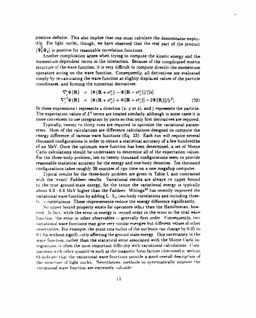
t(’JP Wq) is positive for reasonable correlation functions..Another complication arises when trying to compute the kinetic energy and the

momentum-dependent terms in the interaction. Because of the complicated matrixstructure of the wave function, it is very difficult to compute directlv the momentumoperators acting on the wave function. Consequently, all derivatives are evaluatedsimply by re-calculating the wave function at slightly displad valu~ of the particle

coordinates, and fcrming the numerical derivatives:

V; UI(R} = [IU{R+cf; } - III{R- ci; }]/[’2t]

V;2W{R} = [Q{ R+ct; } + 4{ R-cF; }] -2 UJ{R}]/[C7. (29)

In thee expr~sions i represerits a direction (x, y or z), and j reprments the particle.The expectation values of L2 terms are treated similarly, although in some cases it ismore convenient to use integration by parts so that only first derivatives are required.

Typically, twenty to thirty runs are required to optimize the variational param-eters. !tlost of the calculations are difference calculations designed to compute thecmergy difference of various wave functions (Eq. 23), Each run will require severalthousand configurations in order to obtain a statistical accuracy of a few hundredthscf an \feV, Once the optimum wave function has bem determined, a set of \lonteCarlo calculations should be undertaken to determine all of the expectation values.For the three- body problem, ten to twenty thousand configurations seem to providere~onable statistical accuracy for the energy and onehody densities. Ten thousandt:onfi,gurations takes roughly 30 minutes of cpu time on a one megaflop corr,puter,

“rypical results for the three-body problem are given in Table L and contrastedwii.h the ‘exact’ Faddeev results, Variational results are always sn upper boundto the true ground-state energy, for the triton the variational energy is typicallyilbo~lt 0.;3 - 0.6 YleV higher than the Faddeev. Wiringa2s has recently improved thevariational wave function by adding L . S,, two-body correlations and including thrce-1)! ;.’ correlations, These improvements reduce the energy difference significantly.

So I]l)por hound property exists for operators other than the Hamiltonian, how-l*vm. II) fact, while the error in energy is wwx.mdorder in the error in the trial wave(Iln([.iu[l. the error in other observable Ii generally first order. Consequently, tw()

\;\rliitlo[),ll wave functions may give verv qinlilar mwrgitw but dilfermt values of olherl)im’rv:~blw+, For ~xample, the puint rms r,a(iius of the nuclmms c,an change by 0,05 tu[).I fln without signifil ,;ntly afiecti[lg t,hr ground state energy. ‘l’his uncertainty in thr

wave’ fll[l[ti~m, rfither than the statistical error associated with the Nlontc C’arlo ill-t.(igriitio[l~, is tjftwl the Inmit import~ut ~liliiclllt,y with variational calclllaticms. ( ‘~)nl-[)iirisol]s WI I,tI of,h~~r~lllantit;ns such M thr Ilmgnrtic form factors (discllss~l il. sect.i(mI;) ill(li(’;~fr I I]ilt I Ilc variational wave fl]nrt,io[ls prt)vi~l~ a qoo(l iwfvall IIescrip’ ion ()[I.llr slrl]~”lIlrf’ t~f light nuclri. ~pv,.rtll(sl{*~, l,lf.tll,,,j~ t,] ~ywt~tlll~tical]y illlprt>vv f 1]1*

J ilrialiol]ill wavv fllnctioll are ~xtrmnrly Villllal)lt’

I:{

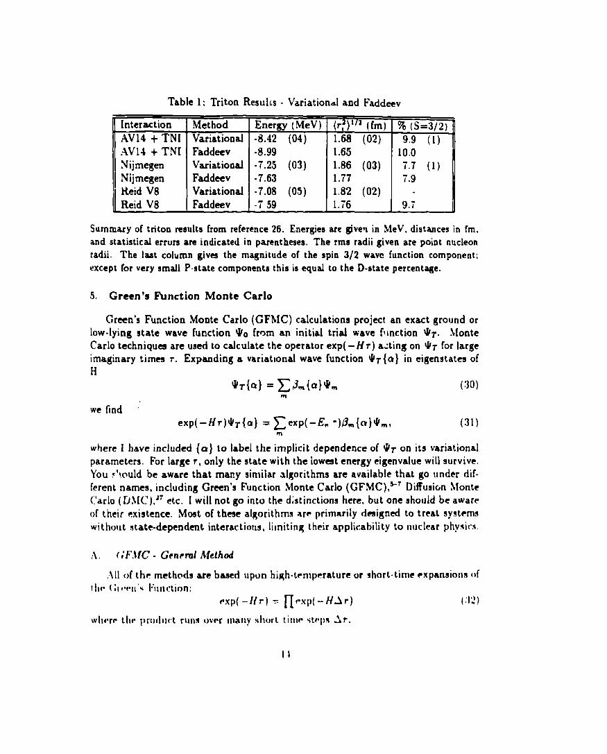
Table 1: Triton Results - Variational and Faddeev

Interaction

~V14 + ‘1’N[.4V14 + T!W~ijmegenLYijmegenReid V8Reid V8

MethodVariationalFaddeevVariationalFaddeevVariational

Faddeww

Energy ( .MeV) (r~)’i’ (fro) ?%(s=3/~)

-8.42 (04) 1.68 (02) 9.9 (1)-8.99 1.65 10.0-7.25 (03) 1.86 (03) 7.7 (1)-7.63 1.77 7.9-7.06 (05) 1.82 (02) .-7 59 1.76 9.7

Summary of triton results from reference 26. Energies arc given in MeV, distances in fm.and statistical errurs are indicated in parentheses. The rms radii given are point nucleonradii. The Iwst column gives the magnitude of the spin 3/2 wave function component:except for very small P-state components this is equal to the D-state percentage.

5, Green’s Function Monte Carlo

Green’s Function Monte Carlo (GFMC) calculations project an exact ground orlow-lying state wave function *o from an initial trial wave f!mction *T, MonteCarlo techniqu~ are used to calculate the operator exp( - kfr) acting on WT for largeimaginary times r. Expanding a variational wave function WT{a} in eigenstates ofH

w~{a} = ~Jm{a}ufm (30)WI

we findexp(-Hr)Or{a} = ~exp(-E. ‘)flm{a}~m, (31)

m

where 1 have included {a} to label the implicit dependence of I#r on its variationalparameters. For large r, only the state with the iowat energy eigenvalue will surviveYou ~’vm.dd be aware that many similar algorithms are available that go under dif-ferent names, including Green’s Function Monte Carlo (GFMC),*7 Diffusicm Monte(.’arlo ( D\[C),J7 etc. I will not go into the distinctions here, but one should be awareof their existence. Most of these algorithms are primarily rimigned to treat systemswithout state-dependent interactions, Iilniting their applicability to nuclear physirs.

upon high- trrnperature or short-time ●xpmnsions of

Of course we I-10not know even the short-time propagator exactly; the exactform would re{~uire imply a knowledge of all eigenstates. However. for short timesteps Jr we can construct accurate approximations to the propagator. The simplest

approximation 1s:

G(R’, RJ = (R’lexp(-H.3r)lR)

~ exP(-L’(R)Ar/2) (R’lexp(-TAr)lR) exp(-V(R’)~r/2), (33)

where I have split the Iiamiltonian into its kinetic (T) and potential (V) pieces andusurnecl that the potential is local.

Green’s Function Monte Carlo is similar in many respects to a transport \lonteCarlo simulation. The basic idea is choose an initial set of configurations with densityproportional to a trial wave function, and to use Monte Carlo methods to iterate anintegral equation:

~l+l(R~) =!

dRG(R’, R) V’(R) (34)

until convergence to the ground state wave function. Each configuration is an in-dependent copy of the entire system, and their “trajectories’ are followed as Eq. 3-Iis iterated, The kinetic energy term allows the sampled points to move about inconfiguration space while the potential energy duplicates or destroys walks.

The Monte Carlo simulation mimics a diffusion process in which the kinetic energyterm governs the rate of the diffusion, since:

[1(R’[ exp( -TAT)IR) = .Vexp ‘(4RL-A~’)2 ,

2m J

I “1

u you can see by expanding the exponential. However, the overall error is propor.tional to ~r, = the total number of steps required to pro~agate a giver imaginary

time is proportional to l/~r,CFMC methods are closely related to the finite-temper~ture simulations in con-

densed matter (Path Integra12e and Fermion \lonte Carlom J and lattice QCI). These

methods retain the complete history of the system over time (its world-line or path),and evaluate

(0) = ~R(ROexp(-3ff)R)

~R(Rexp(-JH)R) “(36)

to determine the expectation value of an operator 0 at an inverse temperature3. Clearly, this e~pression is of the form of Eq. 14, and can be evaluated usingYletropolis Monte Carlo to Iample over all paths. Note that the pattis are closedsince they begin and end al the same point R. The fact that the complete ‘time’history must be retained typically limits thae methods to = 50-100 steps in inversetemperature.

Here, however, we are particularly interested in projecting out specific quantumstat=, We can use this to our advantage and build in our knowledge of the approx-imate ●igenstates, The baaic technique is called ‘importance sampling.’ Jlultiplyingand dividing Eq. 34 by an Importance funclion *1, we obtain

WI(R’)W+l(R’) =H

dR WI(R’)G(R’, R)-~Q,(R) 1VOW’, (37)

where the quallt. ity in brackets is d~ignated the importance sampled Green’s fllnr.tion, For bos(I I( ~ystems, WI is usually the optimum trial wave function ~r obtainedin a variational calculation. This cmstruction has the advantage that the ●nergy canIw obtained ~ an average of I#~lfWr/W)V~, and consequently there is no ~tatisti.ral wror In the limit that the trial state is equal to the exact one. Also. using tlw~l)wtral rrprmmtation of the Green’s function we can compute the total number of~il[llpl~~ /(R) generatd by a point originally at R:

1(;

where Go is the fr~particle propagator for the A-body system, g,, is the tw~bodypropagator including the interaction, and go,, is the two-body free propagator. Thefree particle propagator? are just normalizd gaussians:

Go(R’, R) = .V exp[-(R’ - R)z

4JrliJ/(?m) 1

!fJ ( ‘:J ~ ‘IJ J = .\’’exp[ *],.

The lowest order approximation to the ratio of two-body propagators r~overs Eq.33. The exact two-body Green’s function, though, can be cvaluaceci m an averageover all gaussian paths Iin.king r,, and r,. In finite-temperature studia of bulk liquidhelium, Cenerley and Pollock”’m have used this method to determine the Green’sfunction of Eq. 39,

T3e simplest feasible GFMC algorithm can be describd as follows:

Begin with a set of points In configuration space distributed with probabilitydensity VI W’. i+t the zeroth : eration, ~“ is the trial wave function *T (hereassured to be the same aa Wl), so the original set of points can be generatedwith the Metropolis methods described previously,

For each point in the i’th generation R, generate a new point R’ in the 3.4dimensional space by sampling from a normalized approximate Gr=n’s function6( R, R’), In the simplest case, ~ can be taken to be the fr~ particle Green’~function. ,4 better choice, though, is to include some information about th~im@rtance function, for example by including the first derivative of VI(R) li~

(:,

,\ssign each configuration a weight equal to the ratio of the true importanrrsamph. ~ Grmn’s function to the al~proximate Grern’s function f;, ‘rhls ratwis given by ( Fq. 39):

UII(R’)GO(R’, R)II

glJ(r9)! fi, ).

“ “ ~m ,<J g:J(rlJ&)

( ‘l][ll~ute all (~uantltiea of intermt at the 10~~tlOn R’, Ad lrlc!lll!? thrill

11)

II ,L

points, F“orexample, the ●wrgy at ~PWrALlull I IiII

-,u WhR;)lNIT(RJL

{1.!t ‘~r(Rf)UIT(~)

t!te more general csae, both the numerator

and denominator

(44)

,5.

must be evaluated, and the energy is ,V/ fl,

Each weighted configuration is replaced by n copies of the configuration withunit weight, n being chosen to replicate on average the original weight w,. Forexample, if wi is 0.5, choose n to be 1 half the time and O half the time; ifw, is 2.1, keep two copies with 90 % probability and three copies with 10 To

probability.

Steps 2 through 5 are then repeated until convergence, each repetition repre-senting one iteration of Eq. 37. ~ constant can be added to the Hamiltonian tocontrol the growth or decre~e of the population size. If this constant is such thatthe ground state enwgy is precisely zero, the population will remain constant onaverage. One almost never knows the exact energy ir,itially, but the constant canhe adjusted as the calculation proceeds. The growth estimate of the energy can becalculated aa the logarithm of the ratio of population sizes divided by the time stepJr since the ground state eventually dominates Eq. 31. [n fact, this provides a veryimportant consistency check on the calculation. The energy as determined by thegrowth of the population should be consistent with that determined by averagingover the individual points, as in step 4 above,

[t isn’t immediately obvious that the branching step above is necemary. Indm-i,the rtaults obtained by merely retaining the weight factcrs would be identical, onih~crage. to those obtainal with branching, However, the branching process greatlyrmiucrs the statistical error, After many generations without branching the weights~jf a f~w configurations will become much larger than the rest, and most of the(.omputm time will be spent calculating quantiti~ that have very low weights, [~orl.wvllwntlyq sllch a calculation will be very inefficient,

.\s I have mentioned, Grmm’s Function Monte (~arlo algorithm can be con.+tr~l~’tml which eliminate all short time approximations, Such algorithms are sonw.what II I(JW’ compiicatd but have proven to be extremely valuable in condensed mat-Irr ptly~ltw, where they have been used to determine the ground state energy of buik

10 Some analogi~s ran be made which connmt 11~-1II(’ as a fllnction of the dmmity, .lillll~ tIt I)IIM to nuclear physics, aa the h~lium. helium pot~ntial is vmy repulsive ;It.Ilor: ~listancm (due to the pauli principle) ,and w~akly attractiv~ at large distanrrs,I“llf. f; lJ\l(’ and experimental zero -tmmp~raturc rquations of ~tat~ Agree within ap-l}rl}xllllat,~’lv(),I K over a wide range of densities mwompasming both the liquid and

w.1111r!’ul~~lt~.llt4ium is an Fxtremdy ~trungly illtmm.ting qIIi4tituln ~ystmli;and Llw.~qrm’nwilt of IIIP lnany-body r~hwlations wilt} vxperimcntal r-lilts in very ilnprm~IVP. SIIC}I lal(ulatl[ms lypicfdly wiiploy 50 tu IW ntomq rontilwd within a periu(licI}t)x, othrr qlh,~ntifirs, sIIch M the ~trtlctllr~ fllnrli[)n S(k), hav~ Also I)wI1 ror:lplltml

JIIII f’xtrllmil ngrmvlmnt Imtw,ml thti)rrt i{’al AIIIIt-wpmimmtal rmults is achievrvl.

IN

We now turn to fermion problems, which are considerably more difficult, In thepreceding discussions, I have implicitly assumed that the wave function is positivedefinite. The ground state wave function of a fermion system, however, necessarilyinvolves both positive and negative regions because it must be anti-symmetric. In

some lattice problems. notably lattice QCD at zero baryon density and electroniclattice problems at half filling, the fermion problem can be overcome by introducingauxiliary fields which transform the problem into a bosonic equivalent.tw Here I willc~~cern mYself only with continullm problems, however, .Naive]y, the anti-symmetry

can Le treated by writirlg the wave function as the difference of two functions, eachof which is positive definite:

~1 = ~+1 _~-~, (45)

Equation 34 can then be used to iterate each of the two components separately,and the results combined to determine the fermion ground state. When determiningthe expectation values, we will aiways take the overlap with an anti-symmetric trial.function, hence eliminatingenergy stat~ obtained after

any bosonic components in the calculation. The lowest-many iterations will be the fermion ground state.

D-J.,//

t’i~urv 2 ) ~ransimt ~~stimation GFMC for tho Iowvst anti .symmt?tric state in a 1.dimen~iond

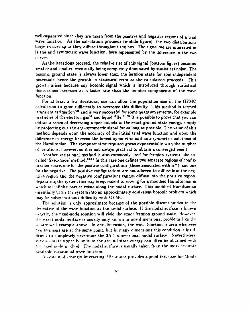
well.~paratd since they are taken from the positive and negative regions of a trialwave functio[,, As the calculation proceeds (middle figure), the two distributionsbegin to overlap as they diffuse throughout the box. The signal we are interested in

is the anti-symmetric wave function, here represented by the difference in the two

curves.As the iterations proced, the relative size of this signal (bottom figure) becomes

smaller and smaller, eventuaUy being completely dominated by stalisticzd noise. Thebosonic ground state is always lower than the fermion state for spin-independentpotentials, hence the growth in statistical error as the calculation proceeds. Thisgrowth arises because any bosonic signal which is introduced through statisticalfluctuations incre~ at a f~ter rate than the fermion components of the wavefunction.

For at Ieaat a few iterations, one can allow the population size in the GFMCcalculation to grow sufficiently to overcome this difficulty, This method is termedtransient ~stimation ’31and is very succmsful for some quantum sy~tems, for examplein studies of the electron gw’a and liquid 3He. ‘lON It is possible to prove that you canobtain a series of decreasing upper bounds to the exact ground state energy, simplyIV projecting out the anti. symmetric signal for aa long as possible. The value of this

method depends upon the accuracy of the initial triaf wave function and upon thedifference in energy between the lowest symmetric and anti-symmetric solutions ofthe Ham.iltonian. The computer time rquired grows exponentially with the numberof iterations. however, so it is not always practical to obtain a converged result,

Another variational method is also commonly used for fermion systems, the sm-called ‘fixed- node’ method .’a’i1 In this case one defines two separate regions of con fig-Ilration space, one for the positive configurations (those associated with W+), and onefor the rmgat ive. The positive configurations are r;ot allowed to diffuse into the neg-,uive region and the negative configurations cannot diffuse into the positive region.Separat illq the system this way is equivalent to solving for a modified Hamiltonian inwhl(.h ~11 I[lfinitp barr& exists along the nodal surface. This modified Hamiltonianmselltially t:]rr,s the system into an approximately quivalent bosonic problem whichmay he Yolved without difficlllty with GFMC,

‘1’lw solution is only approximate because of the possible discontinuities in theIIrrivativt’ of the w~ve function at the mxlal s~Jrface. If the nodal surface is knownI-x,l(’[Iy, tlw fixed-node solution will yield the exact, fermion ground state. How-wr,t Ilr ~’xatt nodal surface is usually only known in one-dimensional problems like tllc<Illl,lrv WPIIexample above. In one dimrmion, the wav function is zrro whenrvclt w!) fl’rl])lons are at the same point, hut in many dimensions this condition is insllf

tirmut f1) wrnpletely determine the 3A-1 dimensional nodal surface. F4evwthdms,wlri ,1~cllr;~tr upper hounds to the grollnd state mwrgy can often be obtained withllIf tix(vl :IIJIIP II IMhoIl, ‘1’he ntxial surf.mr IS Iwually taken frmn the most ~(’~tlri~t~

aVcaIlld)lr v,~rlatlonal wave function.,\ sy~lmll of str(mgly intmarting ‘lie ,ItUIIISprovi(hw a goml lrst ciue for S!iintr

:!()

Carlo algorithms. By employing periodic boundary conditions with different boxsi’zes, one can simulat,e an infinite system of atoms and determine the ground stateenergy as a function of dengity An atom-atom interaction mudel has been developed

by .\ziz,H which consists of a strongly repulsive core region and a weakly attractivetail. The repulsive core arises from the fermi repulsion of the el~trons in the atom,and the attractive tail is a result of electron re-arrangements and is dominamd atlong distance by the atom’s induced dipole moments.

The figure below compares the results of Variational and Green’s Function \lonteCarlo calculations with the experimental equation of state.ll-H .4s can be seen in thefigure, the agreement between GF\IC and experiment is excellent; tile two curvesare within approximately 0, 1 ~ at all densities. The variational rmults are higherthan the GFMC by * 0.3 ~. It is difficult to go beyond an accuracy of * 0.1 KIn these calculations. because at this level finite-size effects and thre-atom forcesbecome important.

Figure J) tjround state rmcrgy per atom versus density f’orliquid ‘He. The ~quareg indicate

variation] \fonte (’MIo calculations, the circles fixed.node ~F\lt~, and the solid line the

,~xprrinll~ntal results.

I!

U_ETJas u u u Lo u

r(oi

Figure 4) Two-body distribution function g(r) for liquid ‘He at experimental equilibriumdensity, The statistical errors in the .Monte Carlo calculation are roughly indicated by thesize of the symbolz.

The GFh4C calculations for bulk 3He employ 54 particla with periodic bound-ary conditions. This is exactly the type of thing we would like to do in nuclearphysics. The equation of state of nuclear matter (even at zero temperature) is a veryimportant quantity, as are measurements of twebody distl ibution functions. Dueto the complexities of the nuclear interaction. though, we are currently limited tostudying very light nuclei. GFMC calculations with state-dependent interactions aredescribed. in t~e next section,

B. GF,VC - ,~pplications to Light iv(idei

The primary complication that arises in nuclear physics GFMC calculations isthe state-dependence of the interaction. The potential, and hence the pair Green’sfunctions ( Zq. 39), are operators in spin-isospin space. Consequently, we mustemploy generalizations of the previous schemes to perform a Green’s function $lonteC’arlu calculation. For example, importance sampling is more complicate qince thewa,~e function is not a simple number. In addition, the weights in general will not be

ii singk= Ilumlxr (or e~en necessarily real), so branching techniques must be modified,Explicitly evaluating even the pair Green’s function is a rather daunting task

given the fact that it depends upon so many variables, [n addition, the potentialsIwtw(wn [lltf~rent pairs do not commute, so the pair approximation itself breaksflown lmlch lnore rapidly in nuclear physics than in condensed-matter problems. Forlht=sc reasons, we construct approximate pair propagators by constructing ‘sub-paths’Iwtwwn r,, aml r~, to ●valuate gi)(r,,, r:, ). These ~ub-paths are sinlply gaussian paths

,), )--

with fixed end-points, a particular path through points r~j, r~j, etc.proportional to:

has a probability

(46)

where r~, is the fixed initial point and q; is the fixed endpoint. In the limit N=lwe get the original short-time approximation (Eq. 33), and in the limit .ti + n

we can reconstruct the complete pair approximation (Eq, 39). When ,V is a power

of two the path can be easily reconstructed by successive divisions, first sampiing‘/2 and the erldpoints, etc. We typically user.v’2 and then subdividing between r

,V = 8, which is a compromise between accuracy and efficiency in calculating thepair propagator. We also sample several paths hetwcwm ri) and ~j, incorporate ingantithetic sampling techniques23 to reduce the varimce.

.4t this stage there doesn’t appear to be much logic in using sub-paths sincewe could obtain the same effect by simply using a smaller time step i,l the originalequations. The oper~tor algebra enables much greater efficiency, however, when weconsider only one pair of particies at a time. If we fix the positions of the particles,the momentum-independent operators in the interaction form a closed set and we cantrivially exponentiate the potential. ‘s The ratio of true to free particle pair Green’s

functions (Eq. 39) i~ approximated aa:

The operator algebra given in reference 35 can then be employed toratio in terms of the six operators

O: s {l,a,~J,r, r,,a, fl,r,. r,, S,,, Sl,rl r,}

approximate this

(IS)

ami associated coefficients, In forming the full .~-body Green’s function ( Eq. 3!)). we

Ilse a \Ionte (’arlo sampling to symmetrize over the order of pair Green’s functions,

Tht= nllriear interaction also contains three-nucleon and momentum-dependenttwo mIrlHII~ iutertictionq. These interactions are relatively weak, hence the followinqgvnerdi~ation of Eq. 39 can be employed:

l“hr (11’rlt,llIvf’opmators in the L oS,, operator act only on the free-particle Grmm’s

fllrlctmll. \l(m” mx:urate expressions for ( j are possible but difficult to implermmt. l;~lrIIxalnplt=. (’~po[l~lltl,lting ~ie two-pion-~x(.]l(lllgc Lhrm-nuclemn interaction involvf=s a,olll[)li(.,atmi Spin -i.x)spin ~tructure.

The remaining non-local terms are proportional to the square of the momentumoperator, and hence can be described in this method aa a direction-dependent ~ef-fective mass’.= However, the fact that this effective mass depends upon spin andisospin limits our ability to do GFMC calculations, since the basis of the methodis that the Gren”s function can be written as a free-particle Green’s function time

small corrections (of the order of AT). This is no longer true for terms such u LZ

and L. St, !wnce we solve for a simplified Argonne V8 model in which no such termsare present. The Argonne V8 model is constructed to reproduce the deuteron ex-actly, and to reproduce the full S- and P-wave interaction with the exception of thecoupling of P and F waves, The difference between the full interaction model and thesimplified V8 model can then be computed in perturbation theory. This perturbativedkct is fairly small, approximately 0.15 MeV in the triton and 0.9 MeV in the al-pha particle. Improved methods for treating state-dependent non-local interactionswould be extremely va!uable.

The basic GFMC algorithm deac.ibed previou~ly now goes through with a fewfairly straightforward generalizations, Each configuration now consists not only ofthe coordinates of the particles, but also a set of amplitud~ in the various spin- isospinchannels. The amplitudes are productq of the hermitim conjugate of the tria! wavefunction times the amplitude of the true wave function. At each iteration, we firstdivide each amplitude by the hermitian conjugate of *T, hence reconstructing thewave function. Then we construct an approximate spin-independent Grem’s function

G and sample a new point R’ from G(R’, R). One alternative is to choose G to bethe the fr~ A-body propagator tim~ the ratio of central correlations in the trialwave function at the points R’ and R. This choice incorporates an approximate

importance 9ampling.Given the init,ial and final points in configuration ip.ce, we then construct the full

Green’s function in operator form, and calcuiate its effect acting upon the wave func.tion at the initial point. Finally, we multiply each component of the wave functionby the hermitian conjugate of the trial function’s component at the new point. Thiscompletes one iteration of the Green’s function equation. Branching is incorporatedby using the absolute value of the sum of all amplitude in the various channels.

Within each run we iterate approximately 1000 configurations for several hundredto a thuusand generations. Approximately twenty runs are required to accurately

tuwess the statistical errors, so the calculations are quite computer intensive. Thealpha particle calculations typically require 50 - 100 hours of cpu time on a Cray -

X \lP. It may be possible to speed them up by incorporating better approximate ions10 the :\-particle Greens function. and hence allowing larger time steps and feweriteratiorls. The results obtained to date with both Variational and Green’s function\lIJntt~ ( ‘,\rlo methodg are presented in the next s~ction,

6. Results

1 will first pr=ent results from a new set of CFYIC calculations for the alphaparticle with a lhree-nucleon-interaction (TNI).371M The convergence of the GFMC

calculation is demonstrated in figure 5, wh]ch shows the energy plotted as a function

of the total iteration time ~ (Eq. 31). At r = O, the enel gy is equal to the variationalresult, and it quickly drops to the exact ground state energy. In fact, the plot coversonly the initial part of the calculation, up to a total iteration time of 0.012 JleV-l.The actual calculation includes 5 times as many iterations, the horizontal lines in thefigure are statistical error bounds obtained by averaging the resultg betwctn 0.024and 0.060 \leV -1. The convergence of the GFMC SCII‘ion is determined by theaccuracy of the trial wave function u well M the excitati~n structure of the nucleus.

In this cue the variational wave function seems to contain small components of highenergy (short-ranged) excitations, excitations which are rapidly projected out in theGF\lC method.

;~O.oa 0.009 0.000 O.oa O.ou

T (Mw”’).— —. .——...._— —..—— —— .

i;i~llrl’ .I, .\lpha Particle Ground State }lnw~v vs. iteration time r.

l“lw \.ariational wav,’ function used in this ralrlllation was taken from refer~’rim=2[; aIIIl tv;is optirnizd for the Argonne ~’l.! plu~ [’rbana model 7 TNI. C’onscquentl!”.II {iI)rs li~)t i)roville a very good &timate for the ground state energy with the rnodrl+ ‘r.%1. Ivlll(”ll hms a stronger repulsive rompomwt And a weaker two.pion-~xchanq(~t(~rln, ][tj~v[,vrr, r,hr rn~~ radius of this t;lal wave function is very near the Pxit “r,,$lllt. ~l(-llt-eit rt~llllrm ~maller cxtrap~l~tions for the intimates of other propmtim.

I! ill a statist iral sense. and thm~fore grounfl( ;l:\l(l prwlucm a wave function {JII..t

.)r-, b

state energy expectation values other than the energy are extrapolated from ‘mixed’and variational estimat~ via:

(.50)

The extrapolations required wit h the present variational wave function are generally

quite small.The thre-nuclmn-interaction included in these calculations is the Argonne model

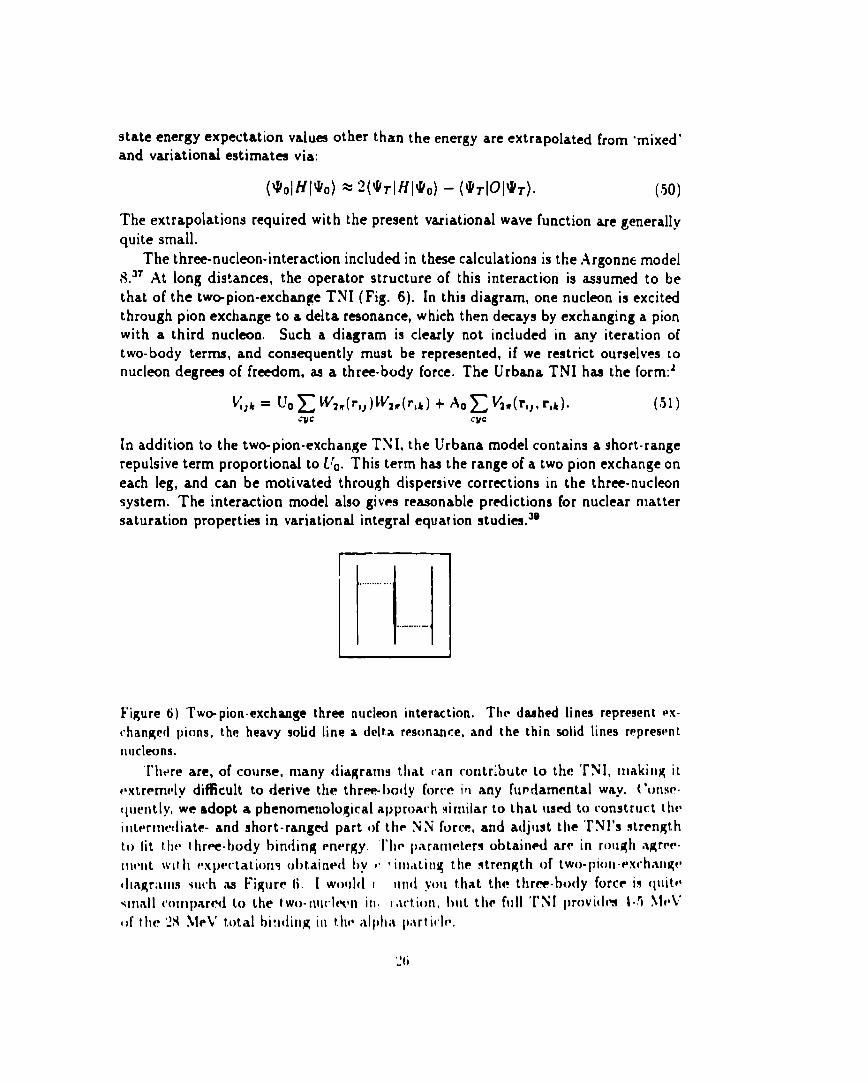
S.37 At long dis!ances, the operator structure of this interaction is assumed to bethat of the tw~pion-exchange T?JI ( Fig. 6). In this diagram, one nucleon is excitedthrough pion exchange to a delta resonance, which then d~ays by exchanging a pionwith a third nucleon, Such a diagram is clearly not included in any iteration oftwo-body terms, and consequently must be represented, if we restrict ourselves conucleon degr~ of freedom, u a three-body force. The Urbana TN I has the form:~

[n addition to the twmpion-exchange TNI, the Urbana model contains a short-rangerepulsive term proportional to Lro. This term has the range of a two pion exchange oneach leg, and can be motivated through dispersive corrections in the thr~-nucleonsystem. The interaction model also gives reasonable predictions for nuclear mattersaturation properties in variational integral equation stud ies.39

.,..... ..

...”....._

Figure 6) Tw-pion-exchartge three nucleon interaction. Thr daohed lines represent Px-

rhanged pims, the heavy solid line a dclr.a resonance, and the thin solid lines represmtnucleons.

‘[’here are, of course, many tiiagrarns that can rorltrlbutr to the TNI, rllaking itt’xtr~m~’ly difficult to derive the three- hmly force in any furdamcntal way. ( ‘urlsfl-(Iuelltly, we adopt a phenomcnological approach ~irlliiar to that USA to mmstrurt thrirlttvmrdiate- and short-ranged part of the Y?i force, and adj~lst the ‘r?J1’s strengthto tit t lie three-body binding t=rwrgy. ‘1.tw paranmtcrs obtained arr in rmlgh agrrr-IIwrlt wll.tl vxpfwtationq obtained hy t’ ?itlli~tillg the strtmgth of twtl-~)loll-~x(.h~~tlqf”

IIlagr:lms such ,as Figurr (i. I WI) III(I I 111111 You that the three- bmly force i~ ~l~llt~’sllinil ro[llparrwi to the t wo- rlll(.lmln irl, i,u”t.iori, l)IIt the flill ‘1’NI provi[lm ,t-5 \lt’\’of thr Y \fek’ total bi:ltling ill tlIf* alplia l)~lrficlf’,

We obtain a ground state energy of -29,20 + 0,15 MeV for the Argonne V8+ TNI model 8 interaction, approximately one ,MeV overbound compared to theexperimental -2S.3 MeV. Employing perturbation thtmry to estimate the differencebetween the Argonne V14 INNinteraction and the V8 model yields 0.9 \leV repulsion,

‘)8.3 + 0.2 MeV, in remarkably good agreement withyielding a total energy of --the experimental result. One should be somewhat cautious because of our use of

perturbation theory in the difference between the V14 and V8 models; but it appearsthat the same three body force can be used to produce very accurate binding energiesfor three and four body nuclei. The Urbana ThII model 8 has been chosen to providea good fit to the triton binding energy, 40 Faddeev results give -8.45 compared corhe experimental .8,48 MeV. We have also attemptd to check cur perturbative

estimate using threebody nuclei, perturbation theory yields very good results but thedifference between V8 and V14 models is only 0.15 MeV for A=3. The expectationvalue of the three nucleon interaction is a small fraction ( < 570) of the total potentialenergy, so at this level there is no apparent re~n to introduce four- or higher-bodyinteraction terms. Other models ( Reid, ?Jijmegen, ,,. ) of the ?JiN potential give a

similar underbidding for the three- and four-body nuclei, hence it should be possibleto lit the binding energies of these nuclei as well with an appropriate T~l model.

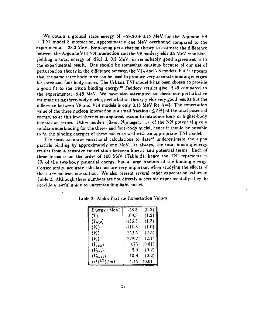
The most accurate variational calculations to date~s underestimate the alphaparticle binding by approximately one JIcV. As always, the total binding energy

results from a qensitive cancellation between kinetic and potential terms. Each ofthese terms is on the order of 100 \leV (Table 2), hence the T~[ reprewnts -.570 of the twebody potential energy, but a large fraction of tile binding energy,( ‘onsequentiy, accurate calculations are very important when studying the etf~~ts ~jfthe t}, re-nucleon intera~tion. We also present several other expectation valu~ ill

I’able 2. :\lthough the~e numbers are not directly at cesslble experimt’ntid]y, they (lo~)rovid~ a useful guide to understanding light nuclei.

. .

“~able 0: Alpha Particle Expectation L’slurs

Energy ( \[cV )(T)

(h/N)(Vw)(v,)(~;)(Ld)(y,-,)(~;-”m)I-’) ’qjm)

10!).:! (!.2).1:1(3.3 (15)Illls (1.0)25’2,5 (’.!,5),),)q ,)-.-!.. (2,1)

0,75 (0.01).3,() ((),2)

1().H ((),2)

l.!: (0,01)

Of particular interest is the strong effect of the tensor interaction in the alphaparticle. With the Argonne ~~ interaction, the tensor components contribute ap-proximately 2/3 of the tw~body potential energy in the alpha particle. Almost

exactly the same fraction is found in Faddeev calculations of threebody nuclei and100.41 The entry V. in the table gives thein cluster Monte Carlo calculations of

contribution of the full one-pion-exchange term in the AV14 interaction, it is almost

equal to the total VN,V expectation value. The Argonne .?JFJinteraction can be writ-ten as a sum of onepion exchange, short range, and intermediate (two-pion ) rangeterms. As shown in the table, there is a strong cancellation between the intermediaterange attraction VI and the short-range repulsion V, in the tw~body interaction.

~\nother me~ure of the strength of the tensor interaction is the D state prob-ability in the four-nuckm ground state. With the Argonne plus Urbana model 8

“1’~1interaction, the D-state probability is 16%, other models range from 12 to 17‘%. These probabilities are nearly consistent with what one would expect based uponthe number of triplet pairs in the A=2, 3, and 4 body nuclei; a ratio of 1:1.5:3.III ddition, th~ -ymptotic D to S state ratio of the alpha particle wave functionIS in good agreement with experimental results .J The remainder of the wave func -r ion is dominated by the fully symmetric S-wave state, which haa a probability of$?.S( 0,2)’Yo. In addition, there are small components of other symmetries, either S-or P-wave,

I

1

O,a 0.0 1,0 u u 8.0

r (mlJ. .... ..—. — — —.——.—.

l’l~llrl’ ~) VM(’ md ( ;FMC results (or thr pr[ltl)n drnslty in [IIF alpha p,wtirl~.

●

does not appear in the variational results. This dip appears in only a very smallfraction ot the total volume because of the ri phase space factor. Nevertheless, itdoes have some consequences when calculating the alpha particle charge form factor.

In the impulse approximation, the charge form factor can be obtained u the fouriertransform of the on~body charge distribution.

[r. reality, though, the eFects of two-body charge and current operators can beimportant even at relatively low momentum transfer. The effects of these two-bodyterms must be included in order to obtain meaningful comparisons with experimentalresults. Riskaa~ has developed a method for constructing models of the exchangecurrents which satisfy the continuity equation:

with an essentially arbitrary two nuclean interaction ~). Terms in the interaction canbe identified which have the appropriate quantum numbers for pion or rho exchange,The continuity equation can then be used to constrain the pi. and rho-exchangeterms in the current, which are called ‘model-independent’ because they are obtaineddirectly from the interaction. In addition, there arc transverse pieces in the current( e.g. .VAy, prr~, and ~r~) which ~re not so constrained, The most importantt,wmbdy terms in the current are due to the pion:

J“(q) = -3i(r, x r,), [i~w(k,)if, (fl, ~k,) - (Ir(k,)a,(dl I k,)-. .

++, k,fl, , k,)[i’q( k,) - i’, (k J]]G;(q),-.I J

wllvre k, is the Illomentllm transferred to nllrlwn i and i’Wi~ the fourier trnnsform

Ill(Pll*, [u t}II*Iiimt of point pions and IIuclcon9..

l{ixkm’wIIW hIMi ddxrminm fi. (k ) AII(I i’,,(k) (Iirm’tlv from thr in~crart ion. III fact,Illis lll,~!ll,)(l [)ro(lu(.w nearly pnlllt-likr i)i- Aml rt)().i)r()[)mqatl)rs with the ,\rg(mtlc*

Il]tf’rm ! 11111.

lo@

1o”’

10”

1O“J

\‘H

: I i

024 @@10

Q(trtr’ )

Figure tla) Magnetic form factor of ‘H, from Schiavilla and Risks.a Impulse approxi.mation (IA) results are shown along with the complete results (IA+tVEC). Curves labeled

F,4D employ the exact Faddeev wave function, and variational results are labeled VAR.

lo~4

. .

1

1o”’ ) \

~ 10’8

!4lo~

\\~ 4tv

I 4

O(tm ‘ )

Figure Ml)) Magnetic form Ilwtl)r (If ‘l{@.ad ab~)v~l

Schiavilla and Riska have computed the magnetic form factors of 3He and 3H(Fig. 8) with this method, as well as the backward cross-section for the electrodisin.tegration O( the deuteron, Several sets of curves are included in the figure, includingresulrs with the impulse currents alone and impulse plus two-body currents, [n addi-

tion, the form factors obtained with \~ariational \[onte Carlo and Faddev methodsare t-ornp,ired. ‘rhe two sets of calculations give very similar results, although there

iire s~me liit~crtinces in the region of the diffraction minimum and beyond, Clearly,the contributions of the exchange currents are crucial to reproducing the experimen-tal results, particularly the contribution of the isovectm exchange current operators.SchiavilIa and Risks have alqo calculated the backward elect rodisintegration of LhcIIeuteron near threshold. This reaction is also very sensitive to the isovertor ex-fhanqe currents, and is well reproduces in the calculations up to very high values of1IN [mmwnturn transfer,

r}wy have also computed the charge form factors of the three-body nuclei44 and(~t)[aln ~ood agreement with experimc’-.al rmults. Exchange corrections to the charge\ jl~llri~(~)r,lrp Tllore qpv( llla~lve sinrc Lhev f“ontairl reliitivistic correct iuns4s iin(i are nut(.(jllstrillfled bv the continuity equation. %[ne of these ambiguities are rlirninatwl in

I tw ,ilplla partlrle howrvc r (Iue to the fact that the alpha particle is an is~w”alar+Vscf’l;l, IVF have combined the followlng lme-body ~’barge operator:

Pi(q) = [1 - -]+[(;~(q)+(f’}(q)rr]

–1 +; ~!fw)-W’,(d + [w(,) - :Gi’,(fd]n}.ll]l”orl)tjr;lrlll~ ttlr [)flrwlf]-~ol(iy I.erln ill)(l ,1 $[11;1111, S corrrrtmn. with il l.V.’t)-l)t IIl\’

s-. ‘** ●0,

n ‘Om2‘1

I3? ,.. -.”’:.:,,,, ,0

b“ ● 8 ●,$*+,;;,??{

●

a II t

I

I

I

I

I

II

++ 1

0.0 1.0 1.0 4.0 Loq (::”’)

*

——. -—. —. —. —... -——

III

—.

Figure 9) VMC arrd GFMC results for one-body and pion contributions to the alphaparticle charge form factor

The full calculations are compared to experimental results in Fig, 10. The (;FNICcalculation is in excellent agreement with experimental resul!s up to a morncntumtransfer of = 4.s fro-l, Beyond that point, the calculated form factor is significantlylarger than experimental results, Nevertheless, the overall agreemmlt is excellentparticularly at lower momentum transfers where one would expect the thtmrv rt)work I)est,

. ..— —— -— .

a

Y

Another very important goal in nuclear physics hss been to obtain an experimen.tal determination of the correlations of nucleons within a nucleus. Inclusive electronscattering experiments can meuure the Coulomb sum, which provides a useful too]

for studving these correlations. The Coulomb sum is defined as:

(57)

where RL is the longitudinal response of the nucleus and GE is the proton form factor.“rhe integral extends from energies just above elastic scattering to infinity, and hence\ve can use closure to calculate the Coulomb sum as a ground state expectation value,

whf!re1 + r,b

~A.(q)= exp(iq orh)[-] (5!))

if we Ignore small neutron contributions (which are included in the calculations) andt wo-bocly terms, [n this approximation, the Coulomb sum is simply:

(60)

wtlrrr }’. is tllr charge form factor of the nucleus and pPP(q) is the frmrier transformof the two-ht~t!y distribution function integrated over the pair’s center-of- maas,

(hulomb Sum

0B

04 LO ha 8!9q (fro’)

.--. —... ----

Figur6 I 1) (’IJulImIIJSIIIIIIn 1110Alpha pwlirll~

:1:1

Thecalculations arecompaed toexperimentd r-ults in Figure 11. ‘l’wo~veat,should be noted concerning this comparison. First, the experimental results onlyextend to a finite energy, and consequently must be extrapolated to deter~ne the[,11]Coulomb sum, Schiavilla et al.4740 calculated the energy- and energy-squaredweighted sun-i ruk with a variatioaal wave function; assumed a functional form for

the response in the tail region, and fit this curve to the calculated moments. The

contributions of tt.e tail region in theexperiment.aregivenM the difference betweenthe points labeled ‘extr’ and ‘trunc’. The latter includes only the raponse up to theexperimental limit. As shown in the figure, the VMC and GFMC curves are nearlyidentical, and both agree very weU with the extrapolated results.

Beckso has extracted pm(q) from the ●~perimental r-ults in the thr~-nucl~nsystem, and obtained the curve shown in Figure 12. He combined the experimentalCoulomb sum and charge form factor, the r=ults of %hiavilla, et al. for the (small)neutron contributions, and a slightly different extrapolation technique to produce theresults shown in the figure. Although th~ qualitative features of the experimentaland theoretical curves are similar, the experimental pm(q) is m’lch higher beyond thefirst minimum. This would indicate even a stronger correlation in the p:otons thanis present theoreticaUy, but contributions of two-body operators to the Coulomb sumshould be included before strong conclusions are drawn.

5

-1—glo% 5

10 25

E“’’l” r T’ 1

i

.

1

LA 1I I \l 1

10-3 L 1 I

o 200 400 600

tigllrr IZ) ‘Fxparimental’ VS. calculatd (~did ~ne) ~m(q), q if ~M~V~from B@ck\”

l’w) Imp{)rtant avenues are open for future research once a consistent piclurpof light nurlri has been obtained, The first of these is calculations of the structureM(1 proprrtlm of heavier nuclei. ~he lnethods I have (Ies(:ribed in these Iecturml.i~n 11P(Iirectly ~xtemied otily IIp h] appro.x)mhtely .4 =t~, and work in this area 1~

*

currently under way, Beyond .+=8, better methods have to be developed to handlethe spin- isospln degrees of freedom in the nucleus. Important progress in this regard

has been made by Pieper et al.,$l who have employed a cluster summation techniqueto study 150. To ciate, variational calculations with the ,4rgonne Vil plus T?iI

model 7 interaction (which is more attractive than m~~’le!8) give approx]mate]y 7

\(e\” binding per nucleon out of the experimental 8 Me~ . They are currently working

on improvements LOboth the variational wave function and the cluster summationmethods. [mpro~ements to the variational wave function incorporate two-body L” Scorrelations N well as improved three-nucleon correlations

The other outstanding problem in the application of lfonte Carlo methods conuclear physics is the study of dynamic properties, a very ambitious goa!, Theprimary successes to date have been in the study of low-energy scattering and elec-tromagnetic transitions, as well as in approximate treatments of dynamic response

52’s3 I will concentrate on the former topic, and particularlyin electron scattering.‘lie - a + ~ reaction,Ilpon the n +

L“ariational \[onte Carlo methods can be employed to study low-energy scatteringin a regime where only two-body breakup is energetically allowed. M The basic idea issimilar to R-matrix approaches, one studi= eigenstates of the Hamiltonian in whichthere is no net flux in or out in any channel. In a onechannel Froblem this amountsto specifying a boundary condition at a radius beyond the interaction region and thenperforrninq a variational calculation to determine the energy eigenvalue associated

with that boundary condition. The boundary condition can take the form of eitherrequiring the relative wave function to be zero at a specific radius,54 or more gene; ally

‘s Determining the eigenvalue M a func:ionrquiring a specific logarithmic derivative.,~f tl~~ bo,~ndary condition is then equivalent to determining the phase shift M a(Ilnct icw of energy.

In principle (; FMC methods can also he usd to study these !ow-energy scatteringl~rol~lmns, and consequently to systematically improve any variational rmu)ts. “rhi~w.hmne can also be generalized to multi-channel scattering proceswa. but rtquires a~{{”trr[lllllatiorlof the energies and relative amplitudes at the channel surfaces. The

[twchod’s practicality depends upon-the ability to cliagonalize in a small biuis ( 10. W+1atISS)IISIIIqS[onte (.arlo methods, Preliminary results on small problems indicat{’I I]at this should IM feasible, but multi-channel methods have not been testd on arf’iilisl ic ~jr(d]lem.

I{’(II\;LWIused this method to study tlw N + ‘ffe ~ n + ~ r~i~ctio~i.’s :\t th~vmi~lf’rlf’rql(w t, his reaction is dominated the spin- 1 s-wave scattering d nrutr~ms on ‘11!’,

I{mvnt lntrr~t in this r~action has cmtmwl m its possibl? rclatiunship to the wmkI’;qJr.11r~ prot-ca irl the four. nuckm svstmr. a rmct ion which produces the kiqhwt1*1)11-!) I)II)t OIWrMovIwutrinos from thd still} I’lwre have hen spm-ulatiuns that thrsr[l(~lltrl[l~]s11)11111 I)r II If*as II~F(l wparmt~ly Ill 11f~ltllrr solar rwutrino Ihwt-vatory. [n ttl(’

illll~lllw’ al)l)roxlliiatiofl,” tlie w~ak itIItj PIIWI r~m~agurtic l-apturr ~i~ \OIOWIV rFlii*(~l,

Ii

Our calculations indicate, though, that the radiative transition igdornjnated bYexchange currents. We obtain a strong-interaction scattering length of 3.5 A 0.25 fm

for the spin one n- 3He state, which agrees well with experimental estimatea. Usingthis scattering wave function and a variational ‘He wave function, we find that only

10 % of the experimental value (60 pbarns)w is obtained in the impulse approxima-tion. The low value is to some extent understandable since the impulse cross section

is precisely zero in the limit where there is no tensor force, and consequently a purelys-wave alpha particle.

Using the full exchange current models, we find a value of 110 pbarns for thecross section, Including only the ‘model-independent’ terms in the exchange currentsgives 70 pbarns, in much better agrement with the experiment, ,A similar result isobtained if we keep only the n exchange terms, as has been done in the n-d capturecalculations of Friar, Gibson, and Payne;sr and use a cut-off of 5,8 r masses inthe propagator. [n this case we obtain a total cross section which agrees with theexperimental value. Our results are quite sensitive to the scattering length, however,a decrease of 0.25 fm in the scattering length would increase the calculated crosssections considerably. We are currently investigating the application of th~ same

‘He. They have also recently beenmethods to the weak capture of protons onapplied to the d + d + a + y reaction. ss

7. Conclusion

\lonte Carlo methods provide a valuable tool for ~nderstanding the structure andproperties of quantum systems. [ have concentrated on applications to light nucleiin rhese Iecturu, but these methods are equally applicable to other arem of nuclear

physics, includinq hypernucl~i and quark-model physics. In recent y~ars we have de-veloped a remarkably consistent picture of light nuclei with the help of ilonte Carlo

and Fadd~v methods. Realistic nuchxm-nucleon interactions combined with plausi-ble threnucltwxt-interaction models have b=n found to give a good descrip~ion ofthe binding energy of three. and four-body nuclei, The ca.lcula~ions to date empha-size the important role of the tensor force, a primary component of this force beingIiIIe to one-pion-exchange. When couplud with re~cmable models of two-body ●x-

[’hange current. and charge operators, these ‘traditional’ models also give remarlmhlyMood dmcriptions of three- and four- bo{ly rkctromagnetic form factors.

I,ight nuclei combine the advantag~s of relative computational simplicity (mat]y

rva]istlc calculations are practical), with phy~ical complexity, “1’heydfer an impor.fNI. Ialmratory for studying a wide w-wiety of nuclear propertim, including nuclmm

llllrlwm correlations, weak and radiativ~ transitions, rtl= procesrms otfcr a widt?var irty of t,rsts for the nuckar Iianliltoni,wl AIIIIexchange currrnt IIIodels. I!rmvi(w

llllrh’i ~)l[rr tlw ~q)portunity for ~tu[lying ttw l~uclcar interaction in nrgative parity~liit,m An(i vwv nmltrorl. rirh Ilurh’i, whwh ,wr important astmphysically throllKhIIwir (’olllif%:tloll” with nf=utr[}ll *t firs,

:11;

The foremost challenge in the future lies in developing new methods to treatquantum dynamics and incorporating relativistic effects in few-body calculations,Some valuable progress has ben made in both of these areas, but much remains to

be done. Accurate microscopic calculations of the dynamic response of light nuclei

to electromagnetic probes is perhaps the most important goal of the next decade,This work was supported by the U. S. Der . tment of Energy.

Referent=

1.

~,

:1,

4.

.5.

6.

7.

s,

!1.

1[),

II.

12.

1:!.

11,

l-).

lfi,

17

1<.

l!).

J. Lomnitz Adler, V. R. Pandharipande, and R. A. Smith, ?JucI. Phys. A361.399 (1981).

J. Carlson, V. R. Pandharipande, and R. B. W’iringa, Nucl. Phys. A401. .59(1283).

R. Schiavilla, V. R. Pandharipande, and R. B. Wiringa, Nucl, Phys. A449, 219( 1986).

J. Carlson and R. B. W’iringa, Los Alamos preprint LA- UR-90-4 11. to appear inCornputat ional ,Vuclear Ph~stcs, Koonin and Langanke cd., Addison- W’esley.

M. H. Kaloa, Phys. Rev. 128, 17!31( 1!362).

\l. H. Iialog, 1), Levesque and L. L’erlet, Phys. Rev, A9, 217S ( 1!374).

K. E. Schmidt, in .tiodels .nd ,\fethods In Few-Body Physics. Lecture Notes inPhysics 273 (Springer- k’erlag, Berlin. 1!)s7).

K. E. Schmidt. \l, H. Kales, and G. V. Chester, Phys, Rev. Lett, 47, s07 ( 1!)S1).

David, .+. I{use and L’eit Elser, Phys. Rev. Lett. 80, 21531( 19sS).

\l, [[, Kales, \f, :\, Lee, P, A. \Vhitlock and G. L’, Chester. Phys. Rev B24,115 (1!)81).

ft. \l. ~)anolf-aud J. C’arlson, Phys. Rev Lett. 62, 1130 ( 19$9 ).”b.

K. E, %.hmidt ami J. W. Iloskowitz. J. Stat, Phys. 43, 1027 ( 1!M6)

J \V ~ltjskt~wlt,z, ~. E, Schmltjt, \[. ;\, LCC, a[l(l \l, [1, K,ilos, J, (“IIMII, l’lIys.77, :14!) (1982).

K, Ih)w, 4 al., I’hys, RCV.Ldt 61, 170(; ( l!NN),

S, l)yrlnan, rat al., Phys. Ibv. (.’38, S00 ( 1!)88),

K. l$. v(m Rden, et al,, Phys. Hev, (“”41, 10/34 ( 1!)90).

I{. i! fl’irlt]ga, l{. :!. Smith. aIItl 1’14. :\i[lsworth, Phys, I{(*v,C’2!I, IW7 ( l!NI ].

1{ \lm.hlr’i~lf, K. .Illlin(lc, aIIIl (’h, I;lster. Phya, Rep, 149, I ( 1!)S7).

\!. \l. ?Jaglm, 1’ ;\. Nijken. And J. ,1. IICSSwart. [)hy~. I{PV, D17, i’[;~ (l!l~~).

.)1.

C. R. Chen, G. L. Payne, J. L. Friar, and B. F. Gibson, Phys. Rev. C33, Ii40(1986).

J. L. Friar, in ,Vew Vistas in Eiccim-~~uclear Physics , ed. E. L. Tomusiak, H. S.Caplaz and E. T. Dressier, Plenum. 1986.

B. F. Gibson and Bruce H. J. McKellar, Few-Body Systems 3, 143 (1988).

Malvin H. Kales and Paula A. Whitbck, Monte C4Ff0 Methods, VOL L JohnW’iley and Sons, Inc., New York, 1986.

N. Metropolis, A. W. Rosenbluth, M. N. Rosenbluth, A. H. TeUer, and E. Teller.J. Chem.”Phys. 21, 1087 (1953).

R. B. Wiringa, to be published.

J. Carlson, Phys. Rev. C38, 1879

D. M. Ceperley and B. J. Alder, J

D. M. Ceperley and E. L. Pollock,

1988).

Chem. Phys. 81,5833 (1986).

Phys. Rev. Lett. s6, 351 (1986).

E. L. Pollock and D. M. Ceperley, Phys. Rev. 30, 2555 (1984).

D. L. Scalapino and R. L. Su ar, Phys. Rev. Lett. 46,519 (1981), and R. Blanken-becler, D. J. Scalapino, and k . L. Sugar, Phys. Rev. D24, 2278 (1981), and Phys.Rev. B24, 4295 (1981),

M. A, Lee, K. E, Schmidt, M. H. Kaloa, and G. V. Chester, Phys, Rev. Lett. 46,728 (1981).

D. M. Ceperley and B. J. Alder, Phys. Rev, Lett. 45, 566 (1980).

R. M. Panoff, in Condensed ,tiatter Theories, edi~ed by R. Kalia, P. Vashishta.and R, Bishop (Plenum, New York, 1987), Vol. 11.

.

R. A. Aziz, V, P. S. ?Jain, J. S. Cerley, W, L. Taylor, and G. T. .McConville, J.Chem. Phys. 70, 4330 ( 1979).

J, Carlson, Phys. Rev. C36, 2026 ( 1987).

J, Carlson, NucI, Phys. A508, 1~lC ( 1990),

J, [Tarlson, to be published.

J. (.’arlson, presented at the Symposium in Honor of Akito Arima, Santa Fe.Nil, 19W; Loa Alarrm preprint LA. IJR-!30-2258.

11. U. Wiringa, V, Fiks, and A. Fabrocini, Phys. Rev. C38, 1010 ( 1988).

B. F, ( ;ibson, private communication.

Steven C, Pieper, private communication.

[), (), Risks, Physics Scripts, 31, 471 ( 1!185).

:1s

-!3. R. Schiavilla and D. O. Risks, Phys. Lett. B244, 373 (1990).

44. R. Schiavilla, V. R. Pandharipande, and D. O. Rish, Phys. Rev. C41, 309(1990).

45. J. L. Friar, Phys. Rev. C22, 796 (1980), and in Mesons in ~Vw4ei, !4. Rho andD. H. Wilkinson, cd., North-Holland, 1979.

46. W. Kloet and J. Tjon, Phys. Lett. 48B, 419 (1974).

47. R. Schiavilla, A. Fabrocini, and V. R. Pandharipande, Nucl. Phys. A.A73,290(1987).

4S. R. Schiavilla, etaL, ?Jucl. Phys. A473,267 (1987).

49. R. Schiavilla, V, R. Pandharipande, and A. Fabrocini, Phys. Rev. C40, 1484( 1989).

50. D. H. B=k, Phys. Rev. Lett. 64,268 (1990), and LJ.of Ill. preprint (?JPL)-90-006(Panic X11 invited talk, MIT, June 1990).

51. Steven C. Pieper, R. B. Wirings, and V, R. Pandharipande, Phys. Rev. Lett.64, 364 (1990).

52. R. Schiavilla and V. R. Pandharipande, Phys. Rev. C36, 2221 ( 1987).

53. R. Schiavilla, Pily~. Lett. B 21S, 1 ( 1989).

,54. J. Carbon, V. R. Pandharipande, and R. B. Wiringa, Nucl, Phys. A424, 47(1984).

,55. J. Carlson, D, 0. Ridca, R, Schiavilla, and R B, Wiringa, Phys. Rev. C 42, 830(1990).

,56. F. L. H. Wolfs, S. J. Freedman, J. E. .Yelson, M. S. Dewey, and G. L. Gr~.*ne,~,hys. Rev. Lett. 63,2721 ( 1989). . .

57. J. L. Friar, B, F. Gibson, and G. L. Payne, to appear in Phys, Lett. B

,S8. A. Arriaga, R, Schiavilla, and V. R, Pandharipande, U. of [11.preprint.

Appendix

Monte Carlo calculations of light nuclei are performed in a basis of definite third

components of spin and isospin for each particle. Thus, the wave function at a given

point in space can represented as a set of 2AA!/(.~!Z!) complex coefficients. The

simplest case is the deuteron, where:

and@d=(n TpT-p Tn ~). (63

The uncorrelated state @~, then, has only two non-zero coefficients and does notdepend upon the spatial coordinates of the particl~.

This basis of states is convenient bc -ause the spin-isospin operators take a par-ticularly simple form. For example,

u,. u,=2P,; -l, r,, r,= 2P,; -1,

where P,f(r) is a permutation operator in spin (isospin) space. Therefore, the e, . a,and r, . r, operatom acting on a state can be evaluated by only two multiplicationsof a scalar time the wave function rather than by full matrix multiplications. Thepermutation operators at,ove can e~ily be represented u bit manipulations on thearray indices within the computer. For example, the indices corraponding to thespin states of the deuteron can be taken as

wherr the middle column is simply the binary representation of the spin st~tt~.( ‘hmrly, P; acting on state 01 ( 1) gives 10 (2), etc.

III a similar manner, the tensor operator S,, = 3u, “?CJ“F - u,’ a, can be rewrittenI]siug:

u’+ = (7+?.. + m.++ +f7io, (64)

m+ = (fir + lfl”)/’2

f7- = ((7, - lflv)/’2

(7,, .= (7~

Fb = (.r t t~)/r

+. = (r - ly)/r

i,, = (:1/r.

II)

The operators a+ and a. do nothing but raise and lower spins, respectively. Notethat they differ from the usual raising and lowering operators by a normalization;these operators give unit coefficient when they flip a spin. Just as the u, . UJ Ud~i . r, can be represented through permutation operators, the tensor operator can be

represented as combinations of permutation and spin flip operators.In this basis, we can explicitly construct the deuteron wave function. It is given

by:

$d = ~c(r)[l + us(r)(3i~ -l)][nlpl-pTnT]

+f(r)[us(r)(3~o++ -l)][n TpJ+nlp T-p~n J-p JnT]

+f’(r)[us(r)(3~~ -l)][nlp J-p Ln J]. (66)

Wave functiong for larger nuclei are easily constructed through successive operationsof pair correlation operators, The effect of the potential terms acting on the wave

function can he calculated similarly.